Experimental test of the Rosenzweig-Porter model for the transition from Poisson to Gaussian unitary ensemble statistics

Abstract

We report on an experimental investigation of the transition of a quantum system with integrable classical dynamics to one with violated time-reversal (${\mathcal{T}}$) invariance and chaotic classical counterpart. High-precision experiments are performed with a flat superconducting microwave resonator with circular shape in which ${\mathcal{T}}$-invariance violation and chaoticity are induced by magnetizing a ferrite disk placed at its center, which above the cutoff frequency of the first transverse-electric mode acts as a random potential. We determine a complete sequence of $\simeq 1000$ eigenfrequencies and find good agreement with analytical predictions for the spectral properties of the Rosenzweig-Porter (RP) model, which interpolates between Poisson statistics expected for typical integrable systems and Gaussian unitary ensemble statistics predicted for chaotic systems with violated ${\mathcal{T}}\,$invariance. Furthermore, we combine the RP model and the Heidelberg approach for quantum-chaotic scattering to construct a random-matrix model for the scattering ($S$) matrix of the corresponding open quantum system and show that it perfectly reproduces the fluctuation properties of the measured $S$ matrix of the microwave resonator.

I Introduction

In the past four decades, random matrix theory (RMT) [1] experienced outstanding success in the field of quantum chaos, of which the objective is to identify quantum signatures of classical chaos in the properties of quantum systems. Originally, RMT was introduced by Wigner to describe properties of the eigenstates of complex many-body quantum systems. He was the first to propose that there is a connection between their spectral properties and those of random matrices [2, 3, 4, 5]. This proposition was taken up in Refs. [6, 7, 8] and led to the formulation of the Bohigas-Giannoni-Schmit (BGS) conjecture which states that the spectral properties of all quantum systems, that belong to either the orthogonal ($\beta=1$), unitary ($\beta=2$) or symplectic ($\beta=4$) universality class and whose classical analogues are chaotic, agree with those of random matrices from the Gaussian orthogonal ensemble (GOE), the Gaussian unitary ensemble (GUE), or the Gaussian symplectic ensemble (GSE), respectively. On the other hand, according to the Berry-Tabor (BT) conjecture [9], the fluctuation properties in the eigenvalue sequences of typical integrable systems ($\beta=0$) exhibit Poissonian statistics.

The BGS conjecture was confirmed theoretically [10, 11] and experimentally, e.g., with flat, cylindrical microwave resonators [12, 13, 14, 15, 16]. Below the cutoff frequency $f^{cut}$ of the first transverse-electric mode the associated Helmholtz equation is scalar, that is the electric field strength is parallel to the resonator axis and obeys Dirichlet boundary conditions (BCs) along the side wall. Accordingly, there the Helmholtz equation is mathematically identical to the Schrödinger equation of a quantum billiard (QB) of corresponding shape with these BCs and the cavity is referred to as microwave billiard. For generic ${\mathcal{T}}$-invariant systems with chaotic classical counterpart that are well described by the GOE [11], complete sequences of up to 5000 eigenfrequencies [17, 18, 19] were obtained in high-precision experiments at liquid-helium temperature $T_{\rm LHe}=4$ K with niobium and lead-coated microwave resonators which become superconducting at $T_{c}=9.2$ K and $T_{c}=7.2$ K, respectively. The BGS conjecture also applies to quantum systems with chaotic classical dynamics and partially violated ${\mathcal{T}}\,$invariance [20, 21, 22, 23]. These are described by a HDS model interpolating between the GOE and the GUE for complete ${\mathcal{T}}$-invariance violation. Such systems were investigated experimentally in [24, 25, 26, 27] and in microwave billiards [28, 29, 30, 31, 32, 33, 34]. In addition, the fluctuation properties of the scattering ($S$) matrix of open quantum systems with partially violated ${\mathcal{T}}\,$invariance were analyzed and exact analytical results were derived based on the Heidelberg approach for quantum-chaotic scattering [35, 36, 37]. Here, ${\mathcal{T}}$-invariance violation was induced by inserting a ferrite into a microwave billiard with chaotic wave dynamics and magnetizing it with an external magnetic field $B$. Because of the Meissner-Ochsenfeld effect [38] this is not possible at superconducting conditions with a lead-coated cavity [18] which is a superconductor of type I [39]. To avoid the expulsion of the external magnetic field, the cavity used in [34] was made from niobium, a type II [40] superconductor for 153 mT $\leq B\leq$ 268 mT.

We report in this work on the experimental investigation of the spectral properties of quantum systems undergoing a transition from Poisson to GUE employing superconducting microwave billiards and the same procedure as in [34] to induce ${\mathcal{T}}$-invariace violation. They have the shapes of billiards with integrable dynamics. Ferrites are inserted into the cavities in such a way, that integrability is not destroyed as long as they are not magnetized. We demonstrate that magnetization with an external magnetic field $B$ induces above the cutoff frequency of the ferrite ${\mathcal{T}}$-invariance violation and also chaoticity. In fact, we showed in Ref. [41] that above the cutoff frequency the spectral properties of a circular cavity that is loaded with a ferrite material which is magnetized by an external magnetic field perpendicular to the cavity plane, agree with those of a classically chaotic quantum system with a mirror symmetry and completely violated ${\mathcal{T}}\,$invariance. Thus, the magnetized ferrite disk acts like a random potential. The objective is to verify analytical results for the spectral properties of the Rosenzweig-Porter (RP) model [42], which was intensively studied about 3-4 decades ago [43, 44, 22, 45, 46, 47, 48, 23, 49, 50, 51]. Here, we restrict to the RP model which describes the transition from Poisson to the GUE. We would like to mention that in recent years the RP model has come to the fore in the context of many-body quantum chaos and localization since it undergoes on variation of a parameter $\alpha$ a transition from localized states in the integrable limit via a non-ergodic phase which is characterized by multifractal states to an ergodic phase [52, 53, 54, 55, 56, 57, 58, 59, 60, 61, 62]. The fractal phase cannot be attained, and above all, not observed with our experimental setup, because we cannot measure wave functions and the achieved values of $\alpha$ are too small.

Superconductivity of the microwave billiards is crucial in order to obtain complete sequences of eigenfrequencies, however, the construction of such cavities containing niobium parts and the realization of ${\mathcal{T}}$-invariance violation by magnetizing ferrites positioned inside the cavity with an external field is demanding. Therefore, we first performed experiments with large-scale resonators at room temperature with the sector-shaped cavity shown in the upper part of Fig. 1 to test whether we can achieve the transition from Poisson to GUE in such microwave experiments. Due to the large absorption of the ferrites it is not possible to identify complete sequences of eigenfrequencies under such conditions. Yet, another measure for the size of chaoticity and ${\mathcal{T}}$-invariance violation are the fluctuation properties of the $S$ matrix associated with the resonance spectra of a microwave resonator [36, 34]. For the case with no magnetization we analyzed properties of the $S$ matrix of that cavity in Ref. [63] and found clear deviations from RMT predictions. To get insight into the size of chaoticity and ${\mathcal{T}}$-invariance violation achieved with the cavity with no disks, we compared the fluctuation properties of its $S$ matrix with those of a cavity with a chaotic wave dynamics which was realized by just adding metallic disks as illustrated in the lower part of Fig. 1. It is known that, when magnetizing the ferrites, such systems are well described by the Heidelberg approach for the $S$ matrix [64] of quantum systems that undergo a transition from GOE to GUE [65, 36, 37]. Another objective of these experiments was to compare the properties of the $S$-matrix with a RMT model which we constructed by combining the RP model and the Heidelberg approach. In Sec. II we report on the scattering experiments and this RMT model and that describing the transition from GOE to GUE. Then, in Sec. III we present results for the spectral properties of a superconducting circular cavity containing a ferrite disk at the center which was magnetized with an external magnetic field. These experiments were performed at liquid Helium $T_{\rm LHe}=4$ K. Finally, in Sec. IV we discuss the results.

II Experiments at room temperature

II.1 Experimental setup

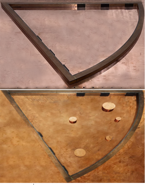
Figure 1: Top: Cavity SB1 without lid. The microwave resonator is composed of a sector shaped frame, shown in the photograph on top of a plate, which forms its bottom, and a top plate as lid. Bottom: Cavity SB2 without lid. It is obtained from SB1 by adding five copper disks of varying sizes and same height as the cavity. All parts are made from copper. To induce partial ${\mathcal{T}}$-invariance violation, three flat rectangular ferrite pieces (black rectangles) of length 50 mm, width 5 mm and height 20 mm were attached symmetrically to both straight parts of the frame at a distance 425 mm, 575 mm, and 725 mm from the apex and magnetized with an external magnetic field of strength 169 mT.

The room-temperature measurements of the $S$ matrix were performed with the large-scale microwave cavity with the shape of a $60^{\circ}$ circle sector used in Ref. [63] and shown without lid in the upper part of Fig. 1. We refer to it as SB1 in the following. The size of the rectangular top and bottom plates are $1260\times 860\times 5$ mm³. The frame has the shape of a $60^{\circ}$ circle sector with radius $R=800$ mm and height $20$ mm corresponding to a cutoff frequency $7.5$ GHz of the first transverse-electric mode. The top and bottom plate and frame were squeezed together tightly with screw clamps. Furthermore, a rectangular frame of the same size as the plates and the same height as the sector frame, and the top and bottom plates were firmly screwed together. Both frames contained grooves that were filled with a tin-lead alloy to improve the electrical contact. Six thin ferrite strips made of 18F6 with a saturation magnetization $M_{s}=180$ mT were attached symmetrically to the straight side walls of the circle sector, to ensure integrability of the wave dynamics for zero external magnetic field [66, 67, 15, 68, 69, 70]. In addition, we inserted five copper disks of varying sizes and same height $20$ mm into the cavity SB1, to induce a chaotic dynamics. We refer to it as SB2 in the following. A photograph of SB2 without lid is shown in the bottom part of Fig. 2.

We checked experimentally for frequencies below $f^{cut}=7.5$ GHz that for the case of non-magnetized ferrites the spectral properties of SB1 [71, 72] and SB2 agree with those of a QB whose shape generates an integrable and chaotic dynamics [73, 74, 75], respectively. The spectral properties of SB2, shown in Fig. 2, agree well with GOE statistics. Those of the empty sector cavity were investigated in [63]. For more details see Secs. III.2 and III.3. Note, that at the walls of the ferrite strips the electric-field strength obeys mixed Dirichlet-Neumann BCs, however, as demonstrated in Refs. [71, 72], the spectral properties of such QBs comply with those of quantum systems with an integrable classical dynamics.

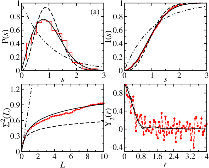
Figure 2: Nearest-neighbor spacing distribution $P(s)$, cumulative nearest-neighbor spacing distribution $I(s)$, number variance $\Sigma^{2}(L)$ and two-point cluster function $Y_{2}(r)$ for the cavity SB2 in the range below the cutoff frequency, which comprises $\approx 500$ eigenfrequencies. They agree well with GOE statistics. The solid, dashed and dashed-dot-dot black lines show the curves for GOE, GUE and Poisson statistics, respectively. For the latter the two-point cluster function equals zero. Therefore it is not shown.

The eigenfrequencies of the cavity correspond to the positions of the resonances in its reflection and transmission spectra. These were measured by attaching antennas $a$ and $b$ at two out of five possible ports distributed over the cavity lid and connecting them to a Keysight N5227A Vector Network Analyzer (VNA) via SUCOFLEX126EA/11PC35/1PC35 coaxial cables. It couples microwaves into the resonator via one antenna $a$ and receives them at the same or the other antenna $b$, and determines the relative amplitude and phase of the output and input signal, yielding the $S$-matrix elements $S_{aa}$ and $S_{ba}$, respectively. To achieve partial ${\mathcal{T}}$-invariance violation we magnetized the ferrite pieces with an external magnetic field $B=169$ mT perpendicular to the cavity plane, generated with NdFeB magnets that were placed above and below the cavity [28, 30, 76, 65]. The absorption at the ferrite surface is especially high for $B\neq 0$ and Ohmic losses in the walls lead to overlapping resonances, which makes the identifacation of their positions challenging. Above all, the wave dynamics is (nearly) integrable implicating close-lying resonances. As a consequence, we were not able to obtain complete sequences of eigenvalues for the normal-conducting resonators with $B\neq 0$ mT. Yet, we succeeded in constructing a superconducting cavity with induced ${\mathcal{T}}\,$invariance, as outlined in Sec. III and, therefore, focused in the room temperature experiments on the fluctuation properties of the $S$ matrix instead. Note that, because we are only interested in properties of the $S$ matrix, we do not need to restrict to the frequency range below $f^{cut}$.

II.2 Random-matrix formalism for the scattering matrix of a quantum-chaotic scattering process

We demonstrated in [63], that the fluctuation properties of the $S$ matrix of the cavity with no ferrites and no or up to three disks, whose spectral properties follow Poisson and intermediate statistics [77], respectively, clearly deviate from those of chaotic scattering systems. Therefore, the question arose how they look like for cavity SB1 for $B\neq 0$. In order to get an estimate for the closeness to a chaotic wave dynamics and the size of ${\mathcal{T}}$-invariance violation we compared its $S$-matrix fluctuation properties to those of the chaotic cavity SB2. For the RMT model describing the fluctuation properties of the $S$ matrix of such cavities exact analytical results exist for the two-point $S$-matrix correlation functions for no or partial up to full ${\mathcal{T}}$-invariance violation in terms of a parameter $\xi$ that quantifies the strength of ${\mathcal{T}}$-invariance violation. We employ them to estimate it for SB1 and determine it for SB2, as outlined in the following.

We performed Monte-Carlo simulations based on the scattering formalism for quantum-chaotic scattering [64]. The $S$-matrix elements of the RMT model, referred to as HDS model in the following,

$$S^{HDS}_{ba}(f)=\delta_{ba}-2\pi i[\hat{W}^{\dagger}\left(f\hbox{$1\hskip-1.2pt\vrule depth=0.0pt,height=6.88889pt,width=0.7pt\vrule depth=0.0pt,height=0.3pt,width=1.19995pt$}-\hat{H}+i\pi\hat{W}\hat{W}^{\dagger}\right)^{-1}\hat{W}]_{ba}.$$ (1)

Here, the matrix $\hat{W}$ accounts for the interaction between the internal states of the resonator Hamiltonian $\hat{H}$, which mimicks the spectral fluctuation properties of the closed microwave cavity, and the open channels. These comprise the two antenna channels $a$, $b$ and $\Lambda$ fictitious ones that account for Ohmic losses in the walls of the resonator [36, 37] in terms of a parameter $\tau_{abs}$. The matrix elements of $\hat{W}$ are real, Gaussian distributed with $W_{a\mu}$ and $W_{b\mu}$ describing the coupling of the antenna channels $a,b$ to the resonator modes $\mu$. We ensured that, as assumed in the HDS model, direct transmission between the antennas is negligible, that is, that the frequency-averaged $S$-matrix is diagonal [78], implying that $\sum_{\mu=1}^{N}W_{e\mu}W_{e^{\prime}\mu}=Nv_{e}^{2}\delta_{ee^{\prime}}$ [78]. The parameters $v^{2}_{e}$ denote the average strength of the coupling of the resonances to channels $e$. For $e=1,\ 2$, referring to the antenna channels, they correspond to the average size of the electric field at the position of the antennas $a$ and $b$ and they yield the transmission coefficients $T_{e}=1-|\left\langle{S_{ee}}\right\rangle|^{2}$, which are experimentally accessible [37]. The transmission coefficients of the ficitious channels, which are assumed to be the same, $T_{3}=T_{4}\dots=T_{\Lambda}=T_{f}$, yield through the Weisskopf formula [79] the absorption parameter $\tau_{abs}=\Lambda T_{f}$. In the numerical simulations we chose $\Lambda=30$.

The transmission coefficients $T_{1},T_{2}$ and $\tau_{abs}$ are input parameters of the HDS model where they are assumed to be frequency-independent. Accordingly, we analyzed the fluctuation properties of the measured $S$ matrix in 1 GHz windows [36]. To determine $\tau_{abs}$ we compared the experimental two-point correlation function

$$C_{ab}(\varepsilon)=\langle S^{\rm fl}_{ab}(\nu)S^{\ast\rm fl}_{ab}(\nu+\varepsilon)\rangle$$ (2)

with $\nu$ and $\varepsilon$ denoting the microwave frequency and frequency-increment in units of the average resonance spacing, to RMT predictions. Generally, $\langle\cdot\rangle$ denotes ensemble and spectral averaging. To get an estimate for the strength of ${\mathcal{T}}$-invariance violation we analyzed cross-correlation coefficients defined as

$$C^{cross}_{ab}(0)=\frac{\mathrm{Re}[\langle S^{\rm fl}_{ab}(f)S^{\ast\rm fl}_{ba}(f)\rangle]}{\sqrt{\langle|S^{\rm fl}_{ab}(f)|^{2}\rangle\langle|S^{\rm fl}_{ba}(f)|^{2}\rangle}},$$ (3)

which provides a measure for the size of violation of the principle of reciprocity, $S_{ab}(f)=S_{ba}(f)$, and thus for the strength to ${\mathcal{T}}$invariance violation. Namely, for ${\mathcal{T}}$-invariant systems the principle of reciprocity holds and $C^{cross}_{ab}(0)=1$, whereas fully violated ${\mathcal{T}}\,$invariance yields $C^{cross}_{ab}(0)=0$.

We constructed a HDS model for the $S$ matrix of cavity SB1 by inserting for $\hat{H}$ in Eq. (1) the Hamiltonian of the RP model which describes the transition from Poisson to the GUE,

$$\hat{H}^{0\to 2}(\lambda=\alpha_{N}/D_{N})=\hat{H}_{0}+\alpha_{N}\hat{H}^{GUE}\,.$$ (4)

Here $\hat{H}_{0}$ is a random diagonal matrix with a smooth but otherwise arbitrary distribution and $\hat{H}^{GUE}$ is drawn from the GUE [80]. To get rid of the $N$-dependence of the parameter $\alpha_{N}$ and to render the limit $N\to\infty$ feasible, which is needed for the derivation of universal, system-independent analytical results for the spectral properties [81, 82], the parameter $\alpha_{N}$ is rescaled with the spectral density of the entries of $\hat{H}_{0}$ [83, 45, 23, 50, 82]. For this it is replaced by $\lambda=\alpha_{N}/D_{N}$, where $\lambda$ gives the value of $\alpha_{N}$ in units of $D_{N}=W/N$, with $W$ denoting the band width of the elements of the diagonal matrix $H_{0}$. The Hamiltonian $\hat{H}^{0\to 2}(\alpha_{N})$ interpolates between Poisson for $\alpha_{N}=0$ and GUE for $\alpha_{N}\to\infty$, however, its spectral properties already coincide with GUE statistics for values of $\lambda$ of order unity. In the numerical simulations we chose $(400\times 400)$ dimensional random matrices with variances $\langle\mathrm{Re}\left(H^{GUE}_{ij}\right)^{2}\rangle=\mathrm{Im}\langle\left(H^{GUE}_{ij}\right)^{2}\rangle=\frac{1}{4N}(1+\delta_{ij})$ and for $\hat{H}_{0}$ Gaussian distributed elements with the same variance as for the diagonal elements of $\hat{H}^{GUE}$. Then, the band width equals $W=2\pi$.

The $S$ matrix properties of cavity SB2 were compared to Monte-Carlo and analytical results for the $S$ model describing the transition from GOE to GUE [84, 36, 37]. For this case $\hat{H}$ in Eq. (1) is replaced by the Hamiltonian [83, 21, 85]

$$\hat{H}^{1\to 2}(\xi)=\hat{H}^{(S)}+i\xi\frac{\pi}{\sqrt{N}}\hat{H}^{(A)},$$ (5)

with the strength of partial ${\mathcal{T}}$-invariance determined by the parameter $\xi$. Here, $\hat{H}^{(S)}$ is a real-symmetric random matrix from the GOE and $\hat{H}^{(A)}$ is real-antisymmetric one with Gaussian distributed elements with mean-value zero and same variance as for $\hat{H}^{(S)}$. For the simulations we chose the same values for dimension and variances as for the Hamiltonian in Eq. (4).

II.3 Analysis of the measured scattering matrix

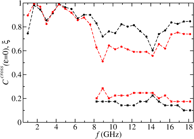
Figure 3: Cross-correlation coefficients of the cavities SB1 (black dots) and SB2 (red dots) determined in 1 GHz windows, where the ferrites where magnetized with an external magnetic field with $B=169$ mT. The corresponding values of the ${\mathcal{T}}$-violation parameter $\xi$ are plotted as black and red squares, respectively (see main text).

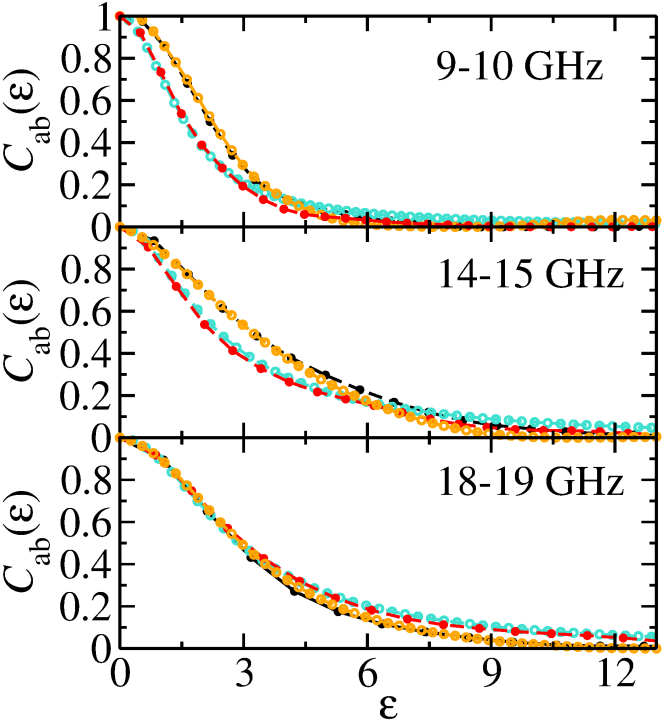
Figure 4: Two-point correlation functions of the $S$-matrix elements for $a\neq b$ in the frequency ranges indicated in the panels. Shown are the results for the cavity SB1 (black) and SB2 (red), the exact analytical results deduced from Eq. (1) with $\hat{H}$ replaced by $\hat{H}^{1\to 2}(\xi)$ (turquoise) and the results obtained from Monte-Carlo simulations for the $S$ matrix Eq. (1) with $\hat{H}$ replaced by $\hat{H}^{0\to 2}(\lambda)$ (orange). The parameters for the transition GOE to GUE are $T_{a}=0.60,T_{b}=0.68,\tau_{abs}=1.6,\xi=0.28$ for $f\in[9,10]$ GHz, $T_{a}=0.80,T_{b}=0.87,\tau_{abs}=2.5,\xi=0.2$ for $f\in[14,15]$ GHz and $T_{a}=0.86,T_{b}=0.89,\tau_{abs}=3.75,\xi=0.185$ for $f\in[18,19]$ GHz. For the transition Poisson to GUE they are $T_{a}=0.60,T_{b}=0.68,\tau_{abs}=0.75,\lambda=0.25$ for $f\in[9,10]$ GHz, $T_{a}=0.80,T_{b}=0.87,\tau_{abs}=2.0,\lambda=0.22$ for $f\in[14,15]$ GHz and $T_{a}=0.86,T_{b}=0.89,\tau_{abs}=3.75,\lambda=0.185$ for $f\in[18,19]$ GHz.

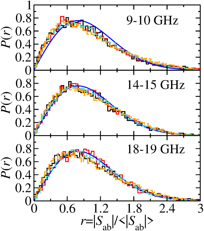
Figure 5: Distributions of the amplitudes of the $S$-matrix for $a\neq b$ in the frequency ranges indicated in the panels. Shown are the results for the cavity SB1 (black) and SB2 (red) and the results of Monte-Carlo simulations for the $S$ matrix Eq. (1) with $\hat{H}=\hat{H}^{1\to 2}(\xi)$ (turquoise) and by $\hat{H}^{0\to 2}(\lambda)$ (orange) for the same parameters as in Fig. 4. The blue solid curve shows the RMT prediction for the Ericson regime of strongly overlapping resonances.

To determine the strength $\xi$ of ${\mathcal{T}}$-invariance violation in the cavity SB2 we proceeded as in [36, 37, 86] and compared the experimental cross-correlation coefficients $C^{cross}_{ab}(0)$, defined in Eq. (3), shown in the right part of Fig. 3 as red dots, to exact analytical results for $C^{cross}(0;\xi,T_{a},T_{b},\tau_{abs})$, yielding the values of $\xi$ shown as red squares in Fig. 3. As outlined in Sec. III.2, the cross-correlation coefficient provides a measure for the size of violation of reciprocity, so that we also used it to find out whether ${\mathcal{T}}$-invariance is violated for the cavity SB1. The results are shown as black dots and squares in  Fig. 3. In order to obtain an estimate for the size of ${\mathcal{T}}\,$invariance violation, we compared the cross-correlation coefficients with the analytical model for the model Eq. (5), even though this is not the appropriate model for SB1. Above about 8 GHz ${\mathcal{T}}\,$invariance is clearly violated.

To determine the value of $\tau_{abs}$ we performed Monte-Carlo simulation for the $S$ matrix Eq. (1) with the model Eq. (4), determined the two-point correlation functions and compared them to the expoermental ones. For the case Eq. (5) we fit the analytical result for the two-point correlation function to the experimental one. In Fig. 4 we compare the experimental correlation functions for the cavities SB1 (black dots) and SB2 (red dots) for different frequency ranges with the Monte-Carlo and analytical results (orange and turquoise), respectively. In Fig. 5 are exhibited the corresponding amplitude distributions. For these no analytical results are available for both models. Agreement between the experimental and RMT curves is very good in all cases. We observe, that with increasing frequency the correlation functions for the cavity SB1 approach those for SB2, implying that there a transition from Poisson to GUE takes place. Thus, magnetization of the ferrite pads induces above the $\approx 8$ GHz ${\mathcal{T}}$-invariance violation and chaoticity of the dynamics, which is above their cutoff frequency. The orange curves, that show the correlation functions and amplitude distributions of the $S$-matrix elements obtained from the HDS model Eq. (1) with $\hat{H}$ replaced by the RP Hamiltonian Eq. (4) agree very well with the experimental ones for the cavity SB1. Thus, we may conclude that this HDS model is appropriate for the description of the fluctuation properties of the $S$-matrix of microwave cavities whose wave dynamics undergoes a transition from Poisson to GUE.

III Experiments at superconducting conditions

III.1 Experimental setup

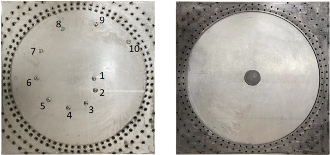
Figure 6: Photograph of the niobium lid (left) and the 5 mm thick lead-coated brass plate with a circular hole on top of a niobium plate (right) of the microwave billiard with a ferrite disk visible at ts center CB1. The lid has been removed.

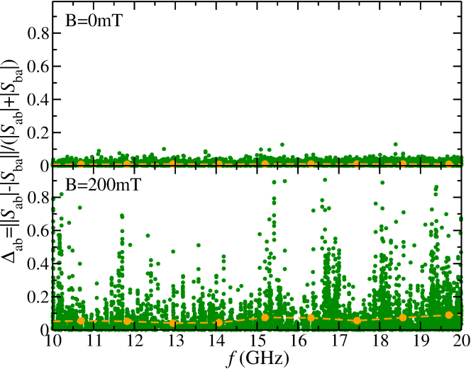
Figure 7: Relative size of violation of the principle of detailed balance for $B=0$ mT and $B=200$ mT, respectively. The orange dots connected by dashed line show the average values in a sliding 1 GHz windows.

We performed experiments at superconducting conditions with a circular microwave billiard, referred to as CB1 in the following, with radius $R=250$ mm containing a ferrite disk with radius $R_{0}=30$ mm at the center, shown in Fig. 6, to investigate spectral properties of quantum systems that undergo a transition from integrable classical dynamics with preserved ${\mathcal{T}}\,$invariance to a chaotic one with complete ${\mathcal{T}}$-invariance violation. The radius of the circle is $R=250$ mm and the cavity height equals $h=5$ mm corresponding to a cutoff frequency $f^{cut}=30$ GHz. A ferrite disk made of 19G3 with saturation magnetization $M_{s}=195$ mT with radius $R_{0}=30$ mm and same height as the cavity corresponding to a cutoff frequency $f_{F}^{cut}\approx 4.5$ GHz is placed at its center. To induce ${\mathcal{T}}$-invariance violation the ferrite is magnetized with a static magnetic field of strength $B=200$ mT that is generated with two external NdFeB magnets, fixed above and below the cavity [34]. In total 10 ports were fixed to the lid. The three plates are screwed together tightly through holes along the cavity boundary and circles visible in the photographs, and tin-lead is filled into grooves that were milled into the top and bottom surfaces of the middle plate along the circle boundary to attain a good electical contact and, thus, high quality factors. To achieve a high quality factors of $Q\gtrsim 5\cdot 10^{4}$, the cavity was cooled down to below $\approx 5$ K in a cryogenic chamber constructed by ULVAC Cryogenics in Kyoto, Japan. We thereby could determine a complete sequence of 1014 eigenfrequencies in the frequency range 10-20 GHz, using the resonance spectra measured between the antennas for all port combinations. The measurements were performed for $B=0$ mT and $B=200$ mT. We also determined the eigenfrequencies of the circular cavity with a metallic disk instead of the ferrite at the center, denoted CB2 in the following. Below $f^{cut}$ it corresponds to an integrable ring-shaped QB.

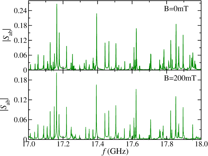
Figure 8: Part of the transmission spectrum of the circular microwave billiard measured at $\approx 5$ K for external magnetic field $B=0$ mT and $B=200$ mT.

In Fig. 7 we show $\Delta_{ab}=[||S_{ab}|-|S_{ba}||]/[|S_{ab}|+|S_{ba}|]$, which gives a measure for the violation of detailed balance, $|S_{ab}|=|S_{ba}|$, and thus for the strength of ${\mathcal{T}}$-invariance violation. Note that for the calibration of the $S$ matrix at superconducting conditions a special cumbersome procedure is required [87, 88, 89] which, however, is not needed as long as one only is interested in spectral properties. Therefore, we cannot get any information on ${\mathcal{T}}$-invariance violation from the fluctuation properties of the $S$ matrix, that depend on its phases, like the cross-correlation coefficients, and considered $\Delta_{ab}$ instead [37]. For $B=0$ mT the principle of detailed balance is fulfilled up to experimental accuracy, whereas for $B=200$ mT it is clearly violated. In Fig. 8 we compare measured transmission spectra of the cavity with a ferrite disk at the center for $B=0$ mT and $B=200$ mT. The effect of magnetization is that the resonances are shifted with respect to those for $B=0$ mT, which becomes visible in a change of the spectral properties as demonstrated in Sec. III.3, and part of them are missing.

III.2 Review of analytical results for the RP model

We analyzed the spectral properties in terms of the nearest-neighbor spacing distribution $P(s)$, the cumulative nearest-neighbor spacing distribution $I(s)$, the two-point cluster function $Y_{2}(r)$, which is related to the spectral two-point correlation function $R_{2}(r)$ via $Y_{2}(r)=1-R_{2}(r)$, the number variance $\Sigma^{2}(L)=\langle(N(L)-\langle N(L)\rangle)^{2}\rangle$, and the form factor $K(\tau)=1-b(\tau)$ with $b(\tau)=\int_{-\infty}^{\infty}Y_{2}(r)e^{-ir\tau}dr$. We compared these measures to analytical ones for the RP model Eq. (4). The parameter $\alpha_{N}$, respectively $\lambda=\alpha_{N}/D_{N}$ characterizing the transition from Poisson to GUE was determined by fitting the result for the number variance $\Sigma^{2}_{0\to 2}(L)$, which was deduced from the exact analytical result for the two-point cluster function $Y_{2}^{0\to 2}(r)$ derived in Refs. [22, 50, 51]. We would like to note, that Georg Lenz derived an analytical expression already in 1992, which is exact for all values of $\alpha_{N}$ and dimensions $N$ of $\hat{H}^{0\to 2}(\lambda)$ in Eq. (4), however, the $N$ dependence is so complex, that the computation of the limit $N\to\infty$ was impossible [22]. In Ref. [50] $Y_{2}^{0\to 2}(r)$ was obtained from the inverse Fourier transform of the analytical result for $b^{0\to 2}(\tau)=\int_{-\infty}^{\infty}Y_{2}^{0\to 2}(r)e^{-ir\tau}dr$,

$$K^{0\to 2}(\tilde{\tau})=1+\frac{2}{\gamma}I_{1}(\gamma)\exp{\left[-\pi\tilde{\alpha}^{2}\tilde{\tau}-\frac{\tilde{\alpha}^{2}\tilde{\tau}^{2}}{2}\right]}$$ (6)

$$-\frac{\tilde{\tau}}{2\pi}\gamma\int_{1}^{\infty}dt(t^{2}-1)I_{1}(\gamma t)\exp\left[-t^{2}\frac{\tilde{\alpha}^{2}\tilde{\tau}^{2}}{2}-\pi\tilde{\alpha}^{2}\tilde{\tau}\right],$$

$$\gamma=\sqrt{2\pi}\tilde{\alpha}^{2}\tilde{\tau}^{3/2},$$ (7)

which was rederived in Ref. [52]. In Ref.[51] an exact analytical expression was computed for $Y_{2}^{0\to 2}(r)$ based on the graded eigenvalue method, yielding

$$Y_{2}^{0\to 2}(r) =\frac{1}{2(\pi r)^{2}}\left[1-e^{-2\frac{r^{2}}{\tilde{\alpha}^{2}}}\cos(2\pi r)\right]-\frac{1}{(\pi\tilde{\alpha})^{2}}$$

$$+\frac{1}{\pi}\int_{0}^{\infty}rdre^{-\frac{r^{2}}{2c}}\int_{0}^{\pi}d\phi\cos(\phi)\left[\mathrm{Re}(A)+\mathrm{Re}(B)\right]$$

$$A =\frac{e^{i\phi}\left[1-\frac{r}{\kappa}\sin\phi\right]}{1+i\frac{re^{i\phi}}{2\kappa}}\exp\left[-i\frac{r^{2}}{2c\kappa}\frac{1}{1-\frac{r}{\kappa}\sin\phi}\right]$$

$$B =\frac{e^{-i\phi}\left[1+\frac{r}{\kappa}\sin\phi\right]}{1+i\frac{re^{-i\phi}}{2\kappa}}\exp\left[-i\frac{r^{2}}{2c\kappa}\frac{1}{1+\frac{r}{\kappa}\sin\phi}\right],$$

$$\kappa =\frac{r}{\pi\tilde{\alpha}^{2}},\,c=\frac{1}{(\pi\tilde{\alpha})^{2}}.$$

Note, that there are discrepancies in the scales of $\tilde{\alpha}$ and $\tilde{\tau}$ between Refs. [49, 50, 82, 52], resulting from differeing definitions of the $N$-independent parameter $\lambda$. We fixed the scales and verified the validity of Eqs. (6)-(9) by comparing the analytical results with Monte-Carlo simulations for spectra consisting of a few hundreds of eigenvalues. We chose $(400\times 400)$-dimensional random matrices, such that the number of eigenvalues is comparable to the experimental eigenfrequency sequences. Here, we used the same settings as in Eq. (4), that is, Gaussian distributed entries for $\hat{H}_{0}$ of the same variance $\langle(\hat{H}_{0})_{ii}\rangle^{2}=\frac{1}{2N}$ as for the diagonal elements $\hat{H}^{GUE}$, such that their band width equals $W=2\pi$, that is, $\alpha_{N}=\lambda D_{N}=\lambda\frac{2\pi}{N}$ in the random matrix model Eq. (4) with a $N$-dimensional Hamiltonian. This yielded $\tilde{\alpha}=\frac{\pi}{\sqrt{2}}\lambda$ and $\tilde{\tau}=\frac{\tau}{\tilde{\alpha}^{2}}$. Note, that approximations have been derived for $Y_{2}^{0\to 2}(r)$ for $\lambda\ll 1$ and $\lambda\gg 1$ in Refs. [43, 44, 22, 45, 46, 47, 48, 23, 49, 50, 51]. These, however, are applicable to the experimental data for a small value of $r$, respectively $L$. Therefore, we do not show the comparison. We determined the values of $\lambda$ from the experimental eigenfrequency spectra by fitting the analytical expression for the number variance deduced from Eq. (9) via the relation

$$\Sigma_{0\to 2}^{2}(L)=L-2\int_{0}^{L}(L-r)Y_{2}^{0\to 2}(r)dr\,,$$ (9)

to their number variance.

In Ref. [22] a Wigner-surmise like expression was derived for the nearest-neighor spacing distribution based on the RP model Eq. (4) with $N=2$, which was rederived in Ref. [90] and is quoted in Ref. [91], given by

$$P_{0\to 2}(s)=Cs^{2}e^{-D^{2}s^{2}}\int_{0}^{\infty}dxe^{-\frac{x^{2}}{4\alpha_{L}^{2}}-x}\frac{\sinh z}{z},\,$$ (10)

$$D(\alpha_{L})=\frac{1}{\sqrt{\pi}}+\frac{1}{2\alpha_{L}}e^{\alpha_{L}^{2}}{\rm erfc}(\alpha_{L})-\frac{\alpha_{L}}{2}{\rm Ei}\left(\alpha_{L}^{2}\right)$$

$$+\frac{2\alpha_{L}^{2}}{\sqrt{\pi}}{{}_{2}{F}_{2}}\left(\frac{1}{2},1;\frac{3}{2},\frac{3}{2};\alpha_{L}^{2}\right),$$

$$C(\alpha_{L})=\frac{4D^{3}(\alpha_{L})}{\sqrt{\pi}},\,z=\frac{xDs}{\alpha_{L}},$$

where erfc$(x)$ denotes the complementary error function, Ei$(x)$ the exponential integral, and ${{}_{2}{F}_{2}}(i\alpha_{1},\alpha_{2};\beta_{1},\beta_{2};x)$ the generalized hypergeometric error function [92, 93]. Comparison of these analytical results with our Monte-Carlo simulations yields $\alpha_{L}=\sqrt{2}\lambda$.

We also analyzed the distribution of the ratios [94, 95] of consecutive spacings between next-nearest neighbors, $r_{j}=\frac{f_{j+1}-f_{j}}{f_{j}-f_{j-1}}$ for which no anayltical results are available. Yet, they have the advantage that no unfolding is requirted since the ratios are dimensionless [94, 95, 96]. Another frequently studied measure is the power spectra, defined as

$$s\left(\tau=\frac{l}{n}\right)=\left\langle\left|\frac{1}{\sqrt{n}}\sum_{q=0}^{n-1}\delta_{q}\exp\left(-2\pi i\frac{l}{n}q\right)\right|^{2}\right\rangle,\,l=1,\dots n$$ (11)

with $n$ denoting the number of eigenvalues and $\delta_{q}=\epsilon_{q+1}-\epsilon_{1}-q$ for a complete sequence of $n$ levels, where $\frac{1}{n}\leq\tau\leq 1$ [97, 98]. An analytical expression was derived for $s(\tau)$ in Ref. [98] in terms of the spectral form factor. It provides a good approximation for experimental data obtained in microwave networks and microwave billiards [99, 32, 100, 101] consisting of sequences of a few hundreds of eigenfrequencies, for all three universality classes of Dyson’s threefold way. With the aim to get an approximation for $s(\tau)$ for the transition from Poisson to GUE, we replaced in the analytical expression of Ref. [98] the spectral form factor by the expression Eq. (6), yet didn’t find good agreement with the experimental data, also not in Monte-Carlo simulations with high-dimensional RP Hamiltonians [102]. Exact analytical results were obtained for the power spectra in Refs. [103, 104] for fully chaotic quantum systems with violated ${\mathcal{T}}\,$invariance, however, we are not aware of any analytical results for the RP model. Due to the lack of an analytical expression we compared the results deduced from the experimental data for the power spectrum to Monte-Carlo simulations, as outlined in Sec. III.3.

III.3 Analysis of correlations in the eigenfrequency spectra

For the analysis of the spectral properties we unfolded the eigenfrequencies to mean spacing one, by replacing them by the spectral average of the integrated resonance density $\langle\mathcal{N}(f)\rangle$, $\epsilon_{i}=\langle\mathcal{N}(f_{i})\rangle$, which for the cavity CB2 is given by Weyl’s formula, $\langle\mathcal{N}(f)\rangle=\frac{\mathcal{A}\pi}{c^{2}}f^{2}-\frac{\mathcal{L}}{2c}f+N_{0}$, with $\mathcal{A}$ and $\mathcal{L}$ denoting the area and perimeter of the billiard, respectively, and provides a good approximation for the cavity CB1 for $B=0$ mT. For $B\neq 0$ mT we determined $\langle\mathcal{N}(f)\rangle$ by fitting a quadratic polynomial to the experimentally determined $\mathcal{N}(f)$. The parameter $\lambda$ was determined in all considered cases by fitting the analytical result Eq. (9) to the experimentally determined number variance, which provides a suitable measure since it is very sensitive to small changes in $\lambda$.

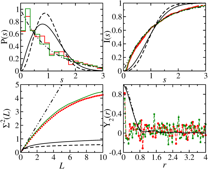
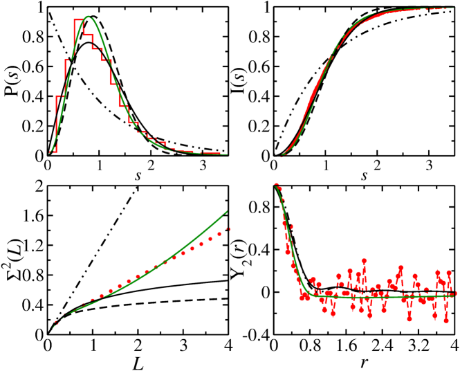
Figure 9: Top: Spectral properties of the cavities CB1 with $B=0$ mT (red histogram and dots) and CB1 (green histogram and squares) for $\approx 1000$ eigenfrequencies in the frequency range [10,20] GHz. They are compared to the results for Poisson (black dashed-dot-dot lines), GOE (solid black lines) and GUE (dashed black lines) statistics. Bottom: Same as top for the cavity CB1 with $B=200$ mT. Here, the green lines show the curves deduced from Eqs. (III.2), (9) and (10) for $\lambda=0.475$.

In the upper part of Fig. 9 we show spectral properties of the cavities CB1 with $B=0$ mT and CB2. The curves lie very close to or on top of each other and coincide with analytical results for the corresponding ring QB, that is, the agreement with Poisson is as good as expected for $\approx 1000$ levels. In the lower part are exhibited the spectral properties for the cavity CB1 with $B=200$ mT in the range $[0,20]$ GHz, which also comprises $\approx 1000$ levels. They agree best with the RP model for $\lambda=0.474$. In Fig. 10 are shown the associated ratio distributions. They are close to Poisson for the case $B=0$ mT and to GUE for $B=200$ mT.

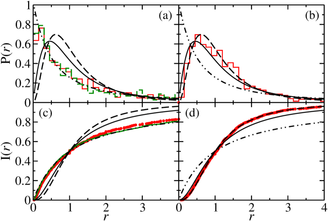
Figure 10: Ratio distributions (upper panel) and cumulative ratio distributions (lower panels). (a), (c): Cavities CB1 (red histogram and dots) amd CB2 (green histogram and squares) for $\approx 1000$ eigenfrequencies in the frequency range [10,20] GHz. They are compared to the results for Poisson (black dashed-dot-dot lines), GOE (solid black line) and GUE (dashed black lines) statistics. (b), (d): Same as (a), (c) for $B=200$ mT.

Actually, using the whole frequency range from 10-20 GHz corresponds to superimposing spectra with different values of $\lambda$. To demonstrate this, we analyzed the spectral properties in frequency intervals of approximately constant $\Delta_{ab}$ (see Fig. 6). They are shown together with the analytical curves in Fig. 11. The corresponding values of $\lambda$ are given in the figure caption. Deviations are visible in the long-range correlations beyond a certain value of $L$. This may be attributed to the comparatively small number of eigenvalues $n$ given in the figure caption. The associated ratio distributions are in all frequency ranges similar to the results shown in Fig. 10 (b) and (d), implying that they are not sensitive to the changes in the value of $\lambda$, i.e., to the size of chaoticity and ${\mathcal{T}}$-invariance violation. Furthermore, we compared experimental results for the form factor to the analytical prediction deduced from Eq. (6). In this case we had to cope with the problem that we have sequences of only few hundreds of eigenvalues, however, for the Fourier transform long sequences are preferable. Furthermore, we have only one sequence for each value of $\lambda$, whereas, e.g. in the experiments [32, 101] an ensemble of up to a few hundreds of spectra of comparable lengths. So we observe a qualitative agreement with the analytical results confirming the values of $\lambda$, however, these data cannot be used to determine $\lambda$. In Fig. 13 we compare the experimentally obtained power spectra to Monte-Carlo simulations with the RP model Eq. (4) and to the curves for the GOE and GUE which were obtained based on the analytical expressions in terms of the form factor derived in Ref. [98]. The smallest value of $\tau$ is $\frac{1}{n}$, with $n$ denoting the number of eigenfrequencies given in the caption. Nevertheless, differences between the power spectra for the different frequency ranges are visible below $\log_{10}(\tau)\simeq-0.5$, and they agree well with the Monte-Carlo simulations.

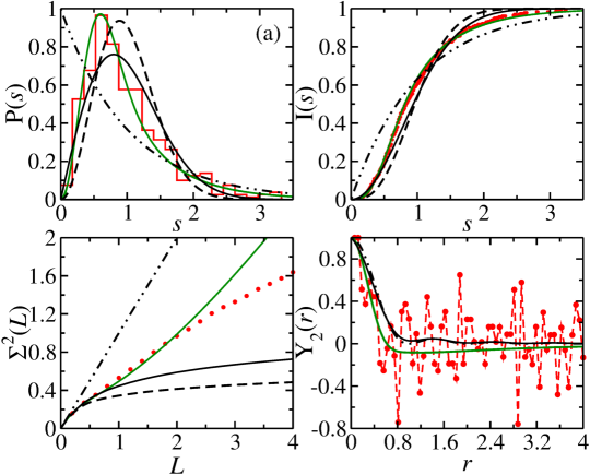
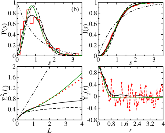
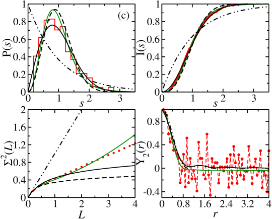
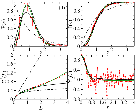
Figure 11: Spectral properties of the cavity CB1 with $B=200$ mT (red histograms and dots). They are compared to the curves deduced from Eqs. (III.2), (9) and (10) (green curves) and results for Poisson (black dashed-dot-dot lines), GOE (solid black line) and GUE (dashed black lines) statistics. Shown are the results for (a) $n=231$, $f_{i}\in[10,13]$ GHz, (b) $n=294$, $f_{i}\in[13,16]$ GHz, (c) $n=232$, $f_{i}\in[16,18]$ GHz and (d) $n=256$, $f_{i}\in[18,20]$ GHz, with $\lambda=0.325,0.45,0.55,0.625$, respectively.

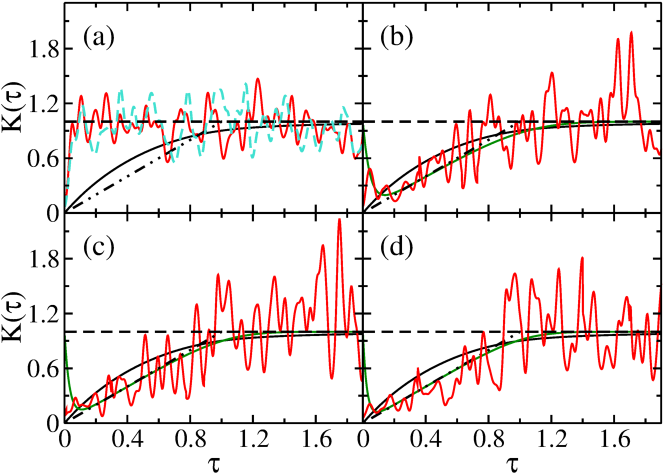
Figure 12: Same as Fig. 11 for the spectral form factor of the cavities (a) CB1 (red solid line) and CB2 (turquoise dashed line) for $B=0$ mT and $\approx 1000$ eigenfrequencies in the frequency range [10,20] GHz and (b)-(d) CB1 with $B=200$ mT (red solid lines) compared to the analytical results Eq. (6) (green curves) and results for Poisson (black dashed-dot-dot lines), GOE (solid black line) and GUE (dashed black lines) statistics. Shown are the results for (b) $n=294$, $f_{i}\in[13,16]$ GHz, (c) $n=232$, $f_{i}\in[16,18]$ GHz and (d) $n=256$, $f_{i}\in[18,20]$ GHz, with $\lambda=0.45,0.55,0.625$, respectively.

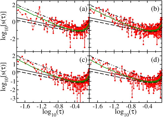
Figure 13: Power spectra for the cavity CB1 with $B=200$ mT (red histograms and dots). They are compared to curves deduced from Monte-Carlo simulations (green curves) and results for Poisson (black dashed-dot-dot lines), GOE (solid black line) and GUE (dashed black lines) statistics for (a) $n=231$, $f_{i}\in[10,13]$ GHz, (b) $n=294$, $f_{i}\in[13,16]$ GHz, (c) $n=232$, $f_{i}\in[16,18]$ GHz and (d) $n=256$, $f_{i}\in[18,20]$ GHz, with $\lambda=0.325,0.45,0.55,0.625$, respectively.

Furthermore, we analyzed length spectra of the three microwave billiard systems. A length spectrum is given by the modulus of the Fourier transform of the fluctuating part of the spectral density from wave number to length and has the property that it exhibits peaks at the lengths of the periodic orbits of the corresponding classical system. The upper part of Fig. 14 shows the length spectra for the cavities CB1 with $B=0$ mT and CB2. Both length spectra exhibit peaks at the lengths of orbits of the corresponding ring QB. Some peaks are either weakened or suppressed for CB1. This is attributed to the differing BCs at the walls of the metallic and ferrite disks, implicating for the latter that in the classical limit there is no specular (hard-wall) reflection at the inner circle. The length spectrum for $B=200$ mT, shown as black curve in the lower part of Fig. 14, some peaks are suppressed or disappear, implying that the corresponding periodic orbits do not exist anymore. These are orbits, that hit the disk at the center of the circular billiard, marked by yellow arrows. Furthermore, we show some periodic orbits. Green arrows point at the corresponding peaks. In Fig. A15 of the appendix we show examples of the electric and magnetic field distributions to illustrate the effect of tye magnetized ferrite, which above its cutoff frequency $f_{F}^{cut}\approx 4.5$ GHz acts like a random potential [41].

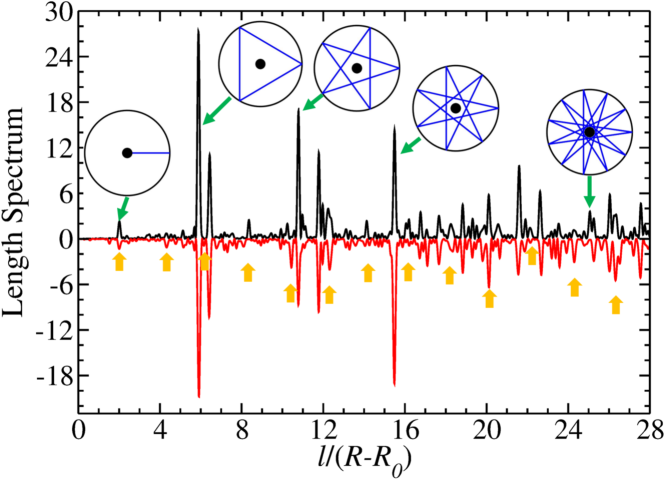
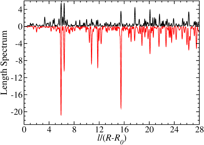
Figure 14: Top: Length spectra of the cavities CB1 (red solid line) and CB2 with radius $R=250$ mm containing a ferrite, respectively metallic disk with radius $R_{0}=30$ mm (black solid line). Orbits, that hit the ferrite disk at the center of the circular billiard and thus feel the differing boundary conditions, are marked by yellow arrows. Green arrows point at the peaks corresponding to the lengths of the orbits shown in the insets. Bottom: Same as top for cavity CB1 with $B=200$ mT (black solid line) and $B=0$ mT (red solid line).

IV Conclusions

We propose an experimental setup – consisting of a flat microwave cavity with the shapes of an integrable billiard, containing ferrite pieces, that are positioned and shaped such that the integrability is not destroyed as long a they are not magnetized – for the study of the properties of typical quantum systems, whose classical counterpart experiences a transition from integrable with preserved ${\mathcal{T}}$-invariance to chaotic with partially violated ${\mathcal{T}}$variance. In Sec. II we demonstrate in room-temperature experiments with a flat circle-sector shaped cavity, that the fluctuation properties of the $S$ matrix associated with the resonance spectrum of such cavities are well described by the Heidelberg approach Eq. (1) with the Hamiltonian replaced by the RP Hamiltonian Eq. (4). Furthermore, in Sec. III we show that the spectral properties of the eigenfrequencies of a circular flat cavity identified in superconducting experiments agree with those of the eigenvalues of the RP Hamiltonian Eq. (4). We confirmed this by comparing them to and thereby verifying analytical results derived in [22, 50, 51]. These experiments were performed with a cavity whose bottom plate and lid are constructed from niobium, a superconductor of type II [40], thereby achieving high-quality factors. This is a crucial prerequisite to render possible the determination of a complete sequence of $\approx 1000$ eigenfrequencies. Thereby, we were able to analyze the spectral properties in various frequency ranges and thus, to observe the gradual transition from Poisson to GUE. Unfortunately, we are not able to measure wave functions with our setup, which relies on Slater’s theorem employing a perturbation body made from magnetic rubber [105] that is moved along the billiard surface with a guiding magnet, which would interfere in the vicinity of the ferrite with the strong magnetic field magnetizing it. However, there the wave functions show clear distortion from those of the integrable billiard as illustrated in Fig. A15. A task for the future is to implement another method which doesn’t use guideing magnets.

V Acknowledgement

This work was supported by the NSF of China under Grant Nos. 11775100, 12247101 and 11961131009. WZ acknowledges financial support from the China Scholarship Council (No. CSC-202106180044). BD and WZ acknowledge financial support from the Institute for Basic Science in Korea through the project IBS-R024-D1. We thank Sheng Xue Zhang who helped with the design of the niobium parts. XD thanks Junjie Lu, who taught him how to do the experiments.

XZ and WZ contributed equally to the work.

Appendix A Examples of electric and magnetic field distributions

In Fig. A15 we show examples for the intensity distributions of the electric-field component $E_{z}$, which for $B=0$ mT corresponds to the wave functions of the ring QB below $f^{cut}=30$ GHz, and for the magnetic-field components $H_{x}$ and $H_{y}$ in the cavity with magnetized ferrite. All other field components vanish below $f^{cut}$. The cutoff frequency of the ferrite disk beyond which the electric field distribution becomes three dimensional, equals $f_{F}^{cut}\approx 4.5$ GHz. We demonstrated in [41], that then the wave dynamics of the disk becomes chaotic and ${\mathcal{T}}$-invariance is completely violated. Thus, above $f=4.5$ GHz it acts like a random potential. This is illustrated in this figure. The distributions were computed with COMSOL Multiphysics. The patterns exhibit clear distortions with respect to those of the corresponding ring-shaped QB. Indeed, as demonstrated for the corresponding spectral properties, the cavity CB1 exhibits above 10 GHz clear deviations from Poisson statistics and is well described by the RP model for the transition from Poisson to GOE.

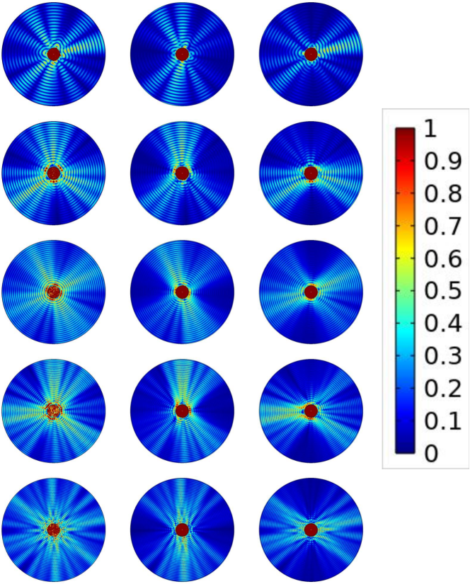
Figure A15: Intensity distributions of the electric field component of the electromagnetic waves along the cavity axis, that is in $z$ direction, $|E_{z}|$, (first column) and the magnetic field components in $x$ and $y$ direction (second and third column), respectively, for, from top to bottom, $f=10.0012,12.9405,16.0522,17.9931,19.9404$ GHz.

References

- Mehta [2004] M. L. Mehta, Random Matrices (Elsevier, Amsterdam, 2004).
- Porter [1965] C. E. Porter, Statistical Theories of Spectra: Fluctuations (Academic, New York, 1965).
- Brody et al. [1981] T. A. Brody, J. Flores, J. B. French, P. A. Mello, A. Pandey, and S. S. M. Wong, Random-matrix physics: spectrum and strength fluctuations, Rev. Mod. Phys. 53, 385 (1981).
- Guhr and Weidenmüller [1989] T. Guhr and H. A. Weidenmüller, Coexistence of collectivity and chaos in nuclei, Ann. Phys. 193, 472 (1989).
- Weidenmüller and Mitchell [2009] H. Weidenmüller and G. Mitchell, Random matrices and chaos in nuclear physics: Nuclear structure, Rev. Mod. Phys. 81, 539 (2009).
- Berry [1979] M. Berry, Structural stability in physics (Pergamon Press, Berlin, 1979).
- Casati et al. [1980] G. Casati, F. Valz-Gris, and I. Guarnieri, On the connection between quantization of nonintegrable systems and statistical theory of spectra, Lett. Nuovo Cimento 28, 279 (1980).
- Bohigas et al. [1984] O. Bohigas, M. J. Giannoni, and C. Schmit, Characterization of chaotic quantum spectra and universality of level fluctuation laws, Phys. Rev. Lett. 52, 1 (1984).
- Berry [1977] M. V. Berry, Regular and irregular semiclassical wavefunctions, J. Phys. A 10, 2083 (1977).
- Giannoni et al. [1989] M. Giannoni, A. Voros, and J. Zinn-Justin, eds., Chaos and Quantum Physics (Elsevier, Amsterdam, 1989).
- Haake et al. [2018] F. Haake, S. Gnutzmann, and M. Kuś, Quantum Signatures of Chaos (Springer-Verlag, Heidelberg, 2018).
- Sridhar [1991] S. Sridhar, Experimental observation of scarred eigenfunctions of chaotic microwave cavities, Phys. Rev. Lett. 67, 785 (1991).
- Stein and Stöckmann [1992] J. Stein and H.-J. Stöckmann, Experimental determination of billiard wave functions, Phys. Rev. Lett. 68, 2867 (1992).
- Gräf et al. [1992] H.-D. Gräf, H. L. Harney, H. Lengeler, C. H. Lewenkopf, C. Rangacharyulu, A. Richter, P. Schardt, and H. A. Weidenmüller, Distribution of eigenmodes in a superconducting stadium billiard with chaotic dynamics, Phys. Rev. Lett. 69, 1296 (1992).
- Deus et al. [1995] S. Deus, P. M. Koch, and L. Sirko, Statistical properties of the eigenfrequency distribution of three-dimensional microwave cavities, Phys. Rev. E 52, 1146 (1995).
- Stöckmann [2000] H.-J. Stöckmann, Quantum Chaos: An Introduction (Cambridge University Press, Cambridge, 2000).
- Richter [1999] A. Richter, Playing billiards with microwaves - quantum manifestations of classical chaos, in Emerging Applications of Number Theory, The IMA Volumes in Mathematics and its Applications, Vol. 109, edited by D. A. Hejhal, J. Friedman, M. C. Gutzwiller, and A. M. Odlyzko (Springer, New York, 1999) p. 479.
- Dietz and Richter [2015] B. Dietz and A. Richter, Quantum and wave dynamical chaos in superconducting microwave billiards, Chaos 25, 097601 (2015).
- Dietz and Richter [2019] B. Dietz and A. Richter, From graphene to fullerene: experiments with microwave photonic crystals, Phys. Scr. 94, 014002 (2019).
- Bohigas et al. [1995] O. Bohigas, M.-J. Giannoni, A. M. O. de Almeidaz, and C. Schmit, Chaotic dynamics and the goe-gue transition, Nonlinearity 8, 203 (1995).
- Pandey and Shukla [1991] A. Pandey and P. Shukla, Eigenvalue correlations in the circular ensembles, J. Phys. A 24, 3907 (1991).
- Lenz [1992] G. Lenz, Zufallsmatrixtheorie und Nichtgleichgewichtsprozesse der Niveaudynamik, Ph.D. thesis, Fachbereich Physik der Universität-Gesamthochschule Essen (1992).
- Guhr [1996a] T. Guhr, Transitions toward quantum chaos: With supersymmetry from poisson to gauss, Ann. Phys. 250, 145 (1996a).
- French et al. [1985] J. B. French, V. K. B. Kota, A. Pandey, and S. Tomsovic, Bound on time-reversal noninvariance in the nuclear hamiltonian, Phys. Rev. Lett. 54, 2313 (1985).
- Mitchell et al. [2010] G. E. Mitchell, A. Richter, and H. A. Weidenmüller, Random matrices and chaos in nuclear physics: Nuclear reactions, Rev. Mod. Phys. 82, 2845 (2010).
- Aßmann et al. [2016] M. Aßmann, J. Thewes, D. Fröhlich, and M. Bayer, Quantum chaos and breaking of all anti-unitary symmetries in Rydberg excitons, Nature Materials 15, 741 (2016).
- Pluhař et al. [1995] Z. Pluhař, H. A. Weidenmüller, J. Zuk, C. Lewenkopf, and F. Wegner, Crossover from orthogonal to unitary symmetry for ballistic electron transport in chaotic microstructures, Ann. Phys. 243, 1 (1995).
- So et al. [1995] P. So, S. M. Anlage, E. Ott, and R. Oerter, Wave chaos experiments with and without time reversal symmetry: GUE and GOE statistics, Phys. Rev. Lett. 74, 2662 (1995).
- Stoffregen et al. [1995] U. Stoffregen, J. Stein, H.-J. Stöckmann, M. Kuś, and F. Haake, Microwave billiards with broken time reversal symmetry, Phys. Rev. Lett. 74, 2666 (1995).
- Wu et al. [1998] D. H. Wu, J. S. A. Bridgewater, A. Gokirmak, and S. M. Anlage, Probability amplitude fluctuations in experimental wave chaotic eigenmodes with and without time-reversal symmetry, Phys. Rev. Lett. 81, 2890 (1998).
- Hul et al. [2004] O. Hul, S. Bauch, P. Pakoński, N. Savytskyy, K. Życzkowski, and L. Sirko, Experimental simulation of quantum graphs by microwave networks, Phys. Rev. E 69, 056205 (2004).
- Białous et al. [2016a] M. Białous, V. Yunko, S. Bauch, M. Ławniczak, B. Dietz, and L. Sirko, Power spectrum analysis and missing level statistics of microwave graphs with violated time reversal invariance, Phys. Rev. Lett. 117, 144101 (2016a).
- Allgaier et al. [2014] M. Allgaier, S. Gehler, S. Barkhofen, H.-J. Stöckmann, and U. Kuhl, Spectral properties of microwave graphs with local absorption, Phys. Rev. E 89, 022925 (2014).
- Dietz et al. [2019] B. Dietz, T. Klaus, M. Miski-Oglu, A. Richter, and M. Wunderle, Partial time-reversal invariance violation in a flat, superconducting microwave cavity with the shape of a chaotic Africa billiard, Phys. Rev. Lett. 123, 174101 (2019).
- Dietz et al. [2007a] B. Dietz, T. Friedrich, J. Metz, M. Miski-Oglu, A. Richter, F. Schäfer, and C. A. Stafford, Rabi oscillations at exceptional points in microwave billiards, Phys. Rev. E 75, 027201 (2007a).
- Dietz et al. [2009] B. Dietz, T. Friedrich, H. L. Harney, M. Miski-Oglu, A. Richter, F. Schäfer, J. Verbaarschot, and H. A. Weidenmüller, Induced violation of time-reversal invariance in the regime of weakly overlapping resonances, Phys. Rev. Lett. 103, 064101 (2009).
- Dietz et al. [2010] B. Dietz, T. Friedrich, H. L. Harney, M. Miski-Oglu, A. Richter, F. Schäfer, and H. A. Weidenmüller, Quantum chaotic scattering in microwave resonators, Phys. Rev. E 81, 036205 (2010).
- Meissner and Ochsenfeld [1933] W. Meissner and R. Ochsenfeld, Ein neuer Effekt bei Eintritt der Supraleitung, Die Naturwissenschaften 21, 787 (1933).
- Onnes [1911] H. K. Onnes, Further experiments with liquid helium. G. On the electrical resistance of pure metals, ect. VI. On the sudden change in the rate at which the resistance of mercury dissappears (Comm. from the Phys. Lab., Leiden, 1911).
- Shubnikov et al. [1937] L. V. Shubnikov, V. I. Ehotkevich, Y. D. Shepelev, and Y. N. Riabinin, Magnetic properties of superconducting metals and alloys, Zh. Eksper. Teor. Fiz. 7, 221–237 (1937).
- Zhang et al. [2023] W. Zhang, X. Zhang, and B. Dietz, T violation and chaotic dynamics induced by magnetized ferrite, Eur. Phys. J. Spec. Top. 10.1140/epjs/s11734-023-00951-0 (2023).
- Rosenzweig and Porter [1960] N. Rosenzweig and C. E. Porter, ”repulsion of energy levels” in complex atomic spectra, Phys. Rev. 120, 1698 (1960).
- French et al. [1988] J. French, V. Kota, A. Pandey, and S. Tomsovic, Statistical properties of many-particle spectra vi. fluctuation bounds on n-nt-noninvariance, Ann. Phys. 181, 235 (1988).
- Leyvraz and Seligman [1990] F. Leyvraz and T. H. Seligman, Self-consistent perturbation theory for random matrix ensembles, J. Phys. A: Math. Gen. 23, 1555 (1990).
- Pandey [1995] A. Pandey, Brownian-motion model of discrete spectra, Chaos, Solitons & Fractals 5, 1275 (1995).
- Brézin and Hikami [1996] E. Brézin and S. Hikami, Correlations of nearby levels induced by a random potential, Nucl. Phys. B 479, 697 (1996).
- Guhr [1996b] T. Guhr, Transition from poisson regularity to chaos in a time-reversal noninvariant system, Phys. Rev. Lett. 76, 2258 (1996b).
- Guhr [1996c] T. Guhr, Ann. Phys. 250, 145 (1996c).
- Altland and Zirnbauer [1997] A. Altland and M. R. Zirnbauer, Nonstandard symmetry classes in mesoscopic normal-superconducting hybrid structures, Phys. Rev. B 55, 1142 (1997).
- Kunz and Shapiro [1998] H. Kunz and B. Shapiro, Transition from poisson to gaussian unitary statistics: The two-point correlation function, Phys. Rev. E 58, 400 (1998).
- Frahm et al. [1998] K. M. Frahm, T. Guhr, and A. Müller-Groeling, Between poisson and gue statistics: Role of the breit–wigner width, Ann. Phys. 270, 292 (1998).
- Kravtsov et al. [2015] V. E. Kravtsov, I. M. Khaymovich, E. Cuevas, and M. Amini, A random matrix model with localization and ergodic transitions, New J. Phys. 17, 122002 (2015).
- Facoetti et al. [2016] D. Facoetti, P. Vivo, and G. Biroli, From non-ergodic eigenvectors to local resolvent statistics and back: A random matrix perspective, Europhys. Lett. 115, 47003 (2016).
- Truong and Ossipov [2016] K. Truong and A. Ossipov, Eigenvectors under a generic perturbation: Non-perturbative results from the random matrix approach, Europhys. Lett. 116, 37002 (2016).
- Monthus [2017] C. Monthus, Multifractality of eigenstates in the delocalized non-ergodic phase of some random matrix models: Wigner–Weisskopf approach, J. Phys. A: Math. Theor. 50, 295101 (2017).
- von Soosten and Warzel [2019] P. von Soosten and S. Warzel, Non-ergodic delocalization in the Rosenzweig-Porter model, Lett. Math. Phys. 109, 905 (2019).
- Pino et al. [2019] M. Pino, J. Tabanera, and P. Serna, From ergodic to non-ergodic chaos in Rosenzweig-Porter model, J. Phys. A: Math. Theor. 52, 475101 (2019).
- Tomasi et al. [2019] G. D. Tomasi, M. Amini, S. Bera, I. M. Khaymovich, and V. E. Kravtsov, Survival probability in Generalized Rosenzweig-Porter random matrix ensemble, SciPost Phys. 6, 014 (2019).
- Bogomolny and Sieber [2018] E. Bogomolny and M. Sieber, Eigenfunction distribution for the Rosenzweig-Porter model, Phys. Rev. E 98, 032139 (2018).
- Berkovits [2020] R. Berkovits, Super-Poissonian behavior of the Rosenzweig-Porter model in the nonergodic extended regime, Phys. Rev. B 102, 165140 (2020).
- Khaymovich et al. [2020] I. M. Khaymovich, V. E. Kravtsov, B. L. Altshuler, and L. B. Ioffe, Fragile extended phases in the log-normal Rosenzweig-Porter model, Phys. Rev. Res. 2, 043346 (2020).
- Skvortsov et al. [2022] M. A. Skvortsov, M. Amini, and V. E. Kravtsov, Sensitivity of (multi)fractal eigenstates to a perturbation of the Hamiltonian, Phys. Rev. B 106, 054208 (2022).
- Zhang et al. [2019] R. Zhang, W. Zhang, B. Dietz, G. Chai, and L. Huang, Experimental investigation of the fluctuations in nonchaotic scattering in microwave billiards, Chinese Physics B 28, 100502 (2019).
- Mahaux and Weidenmüller [1969] C. Mahaux and H. A. Weidenmüller, Shell Model Approach to Nuclear Reactions (North Holland, Amsterdam, 1969).
- Dietz et al. [2007b] B. Dietz, T. Friedrich, H. L. Harney, M. Miski-Oglu, A. Richter, F. Schäfer, and H. A. Weidenmüller, Induced time-reversal symmetry breaking observed in microwave billiards, Phys. Rev. Lett. 98, 074103 (2007b).
- Weaver [1989] R. L. Weaver, Spectral statistics in elastodynamics, J. Acoust. Soc. Am. 85, 1005 (1989).
- Ellegaard et al. [1995] C. Ellegaard, T. Guhr, K. Lindemann, H. Lorensen, J. Nygård, and M. Oxborrow, Spectral statistics of acoustic resonances in aluminum blocks, Phys. Rev. Lett. 75, 1546 (1995).
- Alt et al. [1996] H. Alt, H.-D. Gräf, R. Hofferbert, C. Rangacharyulu, H. Rehfeld, A. Richter, P. Schardt, and A. Wirzba, Chaotic dynamics in a three-dimensional superconducting microwave billiard, Phys. Rev. E 54, 2303 (1996).
- Alt et al. [1997] H. Alt, C. Dembowski, H.-D. Gräf, R. Hofferbert, H. Rehfeld, A. Richter, R. Schuhmann, and T. Weiland, Wave dynamical chaos in a superconducting three-dimensional sinai billiard, Phys. Rev. Lett. 79, 1026 (1997).
- Dembowski et al. [2002] C. Dembowski, B. Dietz, H.-D. Gräf, A. Heine, T. Papenbrock, A. Richter, and C. Richter, Experimental test of a trace formula for a chaotic three-dimensional microwave cavity, Phys. Rev. Lett. 89, 064101 (2002).
- Berry and Dennis [2008] M. V. Berry and M. R. Dennis, Boundary-condition-varying circle billiards and gratings: the dirichlet singularity, J. Phys. A 41, 135203 (2008).
- Bogomolny et al. [2009] E. Bogomolny, M. R. Dennis, and R. Dubertrand, Near integrable systems, J. Phys. A: Math. Theor. 42, 335102 (2009).
- Sinai [1970] Y. G. Sinai, Dynamical systems with elastic reflections, Russ. Math. Surv. 25, 137 (1970).
- Bunimovich [1979] L. A. Bunimovich, On the ergodic properties of nowhere dispersing billiards, Commun. Math. Phys. 65, 295 (1979).
- Berry [1981] M. V. Berry, Regularity and chaos in classical mechanics, illustrated by three deformations of a circular ’billiard’, Eur. J. Phys. 2, 91 (1981).
- Schanze et al. [2001] H. Schanze, E. R. P. Alves, C. H. Lewenkopf, and H.-J. Stöckmann, Transmission fluctuations in chaotic microwave billiards with and without time-reversal symmetry, Phys. Rev. E 64, 065201 (2001).
- Bogomolny et al. [1999] E. B. Bogomolny, U. Gerland, and C. Schmit, Models of intermediate spectral statistics, Phys. Rev. E 59, R1315 (1999).
- Verbaarschot et al. [1985] J. Verbaarschot, H. Weidenmüller, and M. Zirnbauer, Grassmann integration in stochastic quantum physics: The case of compound-nucleus scattering, Phys. Rep. 129, 367 (1985).
- Blatt and Weisskopf [1952] J. M. Blatt and V. F. Weisskopf, Theoretical Nuclear Physics (Wiley, New York, 1952).
- Dietz et al. [2016] B. Dietz, T. Klaus, M. Miski-Oglu, A. Richter, M. Wunderle, and C. Bouazza, Spectral properties of Dirac billiards at the van Hove singularities, Phys. Rev. Lett. 116, 023901 (2016).
- Mehta [1990] M. L. Mehta, Random Matrices (Academic Press London, 1990).
- Guhr et al. [1998] T. Guhr, A. Müller-Groeling, and H. A. Weidenmüller, Random-matrix theories in quantum physics: common concepts, Phys. Rep. 299, 189 (1998).
- Pandey [1981] A. Pandey, Ann. Phys. 134, 110 (1981).
- Dietz et al. [2008] B. Dietz, T. Friedrich, H. L. Harney, M. Miski-Oglu, A. Richter, F. Schäfer, and H. A. Weidenmüller, Chaotic scattering in the regime of weakly overlapping resonances, Phys. Rev. E 78, 055204 (2008).
- Altland et al. [1993] A. Altland, S. Iida, and K. B. Efetov, The crossover between orthogonal and unitary symmetry in small disordered systems: a supersymmetry approach, J. Phys. A: Math. Gen. 26, 3545 (1993).
- Białous et al. [2020] M. Białous, B. Dietz, and L. Sirko, How time-reversal-invariance violation leads to enhanced backscattering with increasing openness of a wave-chaotic system, Phys. Rev. E 102, 042206 (2020).
- Marks [1991] R. Marks, A multiline method of network analyzer calibration, Microwave Theory and Techniques, IEEE Transactions on 39, 1205 (1991).
- Rytting [2001] D. K. Rytting, Network analyzer error models and calibration methods, in Proceedings of the ARFTG/NIST Short Course RF Measurements Wireless World (2001) pp. 1–66.
- Yeh and Anlage [2013] J.-H. Yeh and S. M. Anlage, In situ broadband cryogenic calibration for two-port superconducting microwave resonators, Rev. Sc. Inst. 84, 034706 (2013).
- Kota and Sumedha [1999] V. K. B. Kota and S. Sumedha, Transition curves for the variance of the nearest neighbor spacing distribution for poisson to gaussian orthogonal and unitary ensemble transitions, Phys. Rev. E 60, 3405 (1999).
- Schierenberg et al. [2012] S. Schierenberg, F. Bruckmann, and T. Wettig, Wigner surmise for mixed symmetry classes in random matrix theory, Phys. Rev. E 85, 061130 (2012).
- Abramowitz and Stegun [2013] M. Abramowitz and I. A. Stegun, eds., Handbook of Mathematical Functions with Formulas, Graphs and Mathematical Tables (Dover, New York, 2013).
- Gradshteyn and Ryzhik [2007] I. S. Gradshteyn and I. M. Ryzhik, eds., Tables of Integrals, Series and Products (Elsevier, Amsterdam, 2007).
- Oganesyan and Huse [2007] V. Oganesyan and D. A. Huse, Localization of interacting fermions at high temperature, Phys. Rev. B 75, 155111 (2007).
- Atas et al. [2013a] Y. Y. Atas, E. Bogomolny, O. Giraud, and G. Roux, Distribution of the ratio of consecutive level spacings in random matrix ensembles, Phys. Rev. Lett. 110, 084101 (2013a).
- Atas et al. [2013b] Y. Atas, E. Bogomolny, O. Giraud, P. Vivo, and E. Vivo, Joint probability densities of level spacing ratios in random matrices, J. Phys. A 46, 355204 (2013b).
- Relaño et al. [2002] A. Relaño, J. M. G. Gómez, R. A. Molina, J. Retamosa, and E. Faleiro, Quantum chaos and noise, Phys. Rev. Lett. 89, 244102 (2002).
- Faleiro et al. [2004] E. Faleiro, J. M. G. Gómez, R. A. Molina, L. Muñoz, A. Relaño, and J. Retamosa, Theoretical derivation of noise in quantum chaos, Phys. Rev. Lett. 93, 244101 (2004).
- Faleiro et al. [2006] E. Faleiro, U. Kuhl, R. Molina, L. Muñoz, A. Relaño, and J. Retamosa, Power spectrum analysis of experimental sinai quantum billiards, Phys. Lett. A 358, 251 (2006).
- Białous et al. [2016b] M. Białous, V. Yunko, S. Bauch, M. Ławniczak, B. Dietz, and L. Sirko, Long-range correlations in rectangular cavities containing pointlike perturbations, Phys. Rev. E 94, 042211 (2016b).
- Che et al. [2021] J. Che, J. Lu, X. Zhang, B. Dietz, and G. Chai, Missing-level statistics in classically chaotic quantum systems with symplectic symmetry, Phys. Rev. E 103, 042212 (2021).
- Čadež et al. [2023] T. Čadež, B. Dietz, D. Rosa, A. Andreanov, and D. Nandy, (2023), ”in preparation”.
- Riser et al. [2017] R. Riser, V. A. Osipov, and E. Kanzieper, Power spectrum of long eigenlevel sequences in quantum chaotic systems, Phys. Rev. Lett. 118, 204101 (2017).
- Riser and Kanzieper [2023] R. Riser and E. Kanzieper, Power spectrum of the circular unitary ensemble, Physica D: Nonlinear Phenomena 444, 133599 (2023).
- Bogomolny et al. [2006] E. Bogomolny, B. Dietz, T. Friedrich, M. Miski-Oglu, A. Richter, F. Schäfer, and C. Schmit, First experimental observation of superscars in a pseudointegrable barrier billiard, Phys. Rev. Lett. 97, 254102 (2006).