Quantifying the effect of X-ray scattering for data generation in real-time defect detection

Abstract

X-ray imaging is widely used for non-destructive detection of defects in industrial products on a conveyor belt. Real-time detection requires highly accurate, robust, and fast algorithms to analyze X-ray images. Deep convolutional neural networks (DCNNs) satisfy these requirements if a large amount of labeled data is available. To overcome the challenge of collecting these data, different methods of X-ray image generation can be considered. Depending on the desired level of similarity to real data, various physical effects either should be simulated or can be ignored. X-ray scattering is known to be computationally expensive to simulate, and this effect can heavily influence the accuracy of a generated X-ray image. We propose a methodology for quantitative evaluation of the effect of scattering on defect detection. This methodology compares the accuracy of DCNNs trained on different versions of the same data that include and exclude the scattering signal. We use the Probability of Detection (POD) curves to find the size of the smallest defect that can be detected with a DCNN and evaluate how this size is affected by the choice of training data. We apply the proposed methodology to a model problem of defect detection in cylinders. Our results show that the exclusion of the scattering signal from the training data has the largest effect on the smallest detectable defects. Furthermore, we demonstrate that accurate inspection is more reliant on high-quality training data for images with a high quantity of scattering. We discuss how the presented methodology can be used for other tasks and objects.

[1]organization=Computational Imaging, Centrum Wiskunde en Informatica, addressline=Science Park 123, city=Amsterdam, postcode=1098 XG, country=The Netherlands

[2]organization=Faculteit Wiskunde en Informatica, Technical University Eindhoven, addressline=Groene Loper 5, city=Eindhoven, postcode=5612 AZ, country=The Netherlands

[3]organization=Mathematical Institute, Utrecht University, addressline=Budapestlaan 6, city=Utrecht, postcode=3584 CD, country=The Netherlands

[4]organization=Leiden Institute of Advanced Computer Science, Leiden University, addressline=Niels Bohrweg 1, city=Leiden, postcode=2333 CA, country=The Netherlands

X-ray scattering influences non-destructive inspection performed with X-ray imaging

Scattering signal is an additional noise present in transmission images

Precise deep learning on generated data requires the simulation of scattering

Our methodology compares DCNNs using the size of the smallest detectable defect

We quantitatively evaluate the difference between fast and accurate data generation

1 Introduction

X-ray imaging is used as a non-destructive testing technique that is suitable for objects of different shapes made of various materials (ISO 16371-2:, 2017; Chen et al., 2021b). In this paper, we concentrate on the task of defect detection: a product might contain an undesirable structure (an object made of different material or a void) that should be detected by an inspection system. Detection only refers to indicating that a defect is present and does not require locating it in the studied volume. Examples of defects in this context include spallation in metal alloys, blowholes in casting, razors in airplane baggage, bones in fish fillets, etc. Due to a different density and chemical structure, defects affect an X-ray image (later referred to as projection) of the product. Their presence can be detected by analyzing the projection with an algorithm or a human expert (Fig. 1). One projection can be acquired in tens of milliseconds making X-ray imaging a real-time and in-line inspection technique. While individual projections can be inspected by a human expert, high throughput of data requires a fast and accurate algorithm for defect detection. The main challenge of analyzing X-ray projections is an overlap between features of the object located at different depths. This complicated task is conventionally solved by human experts relying on application-specific knowledge.

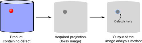
Figure 1: General scheme of defect detection via X-ray imaging. X-ray acquisition system is used to make a projection of the product of interest. Defects affect projection intensity even if they are inside the product, and can be detected by analyzing the projection.

In recent years, deep learning methods, such as deep convolutional neural networks (DCNNs), have been successfully applied in many fields of industrial product inspection (Mery, 2015; Yang et al., 2020; Lee et al., 2021). Deep learning algorithms assume that the image processing task can be solved by a function with a large number of parameters (the exact number depends on the application and can exceed millions for computer vision tasks). The values of these parameters are found by optimizing the result of the function for a large set of projections (referred to as training data). Compared to conventional algorithms for image processing, DCNNs provide higher accuracy at the cost of interpretability. The high predictive power of DCNNs stems from the ability to generalize image patterns in a training dataset. Such datasets, with a few exceptions (Mery et al., 2015), are not available for X-ray defect detection. To circumvent this barrier, experts from different fields have tried simulating X-ray data using computational methods (Bellon and Jaenisch, 2007; Gong et al., 2018). Depending on the desired level of similarity to real data, the methods vary from ray tracing to a Monte-Carlo simulation of every individual X-ray photon.

The computational cost of the simulation algorithm for X-ray imaging comes from the models of X-ray interaction with objects and X-ray registration in the detector. Most methods do not estimate the effect of X-ray photon scattering since it significantly increases the computational complexity of the problem (Gong et al., 2019). Instead, only primary radiation - photons that pass through the object without scattering - is simulated. If the training data are generated only using the primary X-ray signal, the DCNN misses the influence of scattered photons which is present in the real test data. Hence, a drop in accuracy is possible. Due to the low interpretability of DCNNs, it is impossible to predict in advance how a change in the training data would affect the performance on a wide range of test cases. Furthermore, the detection accuracy for any particular test projection depends on many factors such as the properties of that projection and the properties of all projections in the training dataset. Balancing the computational cost of the data generation approach and the resulting DCNN performance requires an accurate and robust metric of detection accuracy. In this paper, we use the Probability of Detection (POD) curves to compare the performance of DCNNs on the varied test data.

We present a methodology that quantitatively evaluates the effect of X-ray scattering in the training data on the accuracy of DCNNs for defect detection in X-ray projections. To demonstrate its application, we perform computational experiments on a model problem that consists of the detection of a cavity inside a cylindrical object. Using a Monte-Carlo simulation algorithm, we produce two versions of the same training data that include and exclude scattered X-ray photons. These data are used to train two DCCNs. We use POD curves to evaluate the correlation between network accuracy and test projection properties. Consequently, we can separate the influence of the training and test data properties and highlight conditions under which the simulation of scattering is crucial. We discuss how this methodology can be applied to other industrial problems and which task properties significantly influence the results.

2 Related work

The problem of defect detection can take different forms depending on the desired output of the algorithm. Classification provides a single label corresponding to the type of defect present in the projection (e.g. steel defects (Masci et al., 2012)). Object detection outputs bounding boxes for every defect and labels corresponding to their types (commonly used in baggage inspection (Aydin et al., 2018) and quality control of metal details such as aluminum castings (Parlak and Emel, 2023)). Segmentation provides a set of pixel masks: every pixel of the projection is labeled if a defect is present there (e.g. spallation in aircraft engines (Bian et al., 2016)). There is a difference between semantic (one mask for all defects of the same type) and instance (different defects of the same type are separated) segmentation. This is not relevant for our model problem where there is only a single defect.

In contrast to color photos, there is a lack of publicly available X-ray projections of industrial products to train and benchmark DCNNs. A notable exception is GDX-ray (Mery et al., 2015) - a dataset containing projections of welds, castings, baggage, and natural objects. Data for a specific defect detection problem have to be either acquired manually or computationally generated. There are two main approaches to the data generation: transforming real projections with image-to-image methods and simulating X-ray imaging. Image-to-image algorithms might be used to add defects to the existing images of objects without defects (Van De Looverbosch et al., 2022). Generative adversarial networks (GANs) can also be used to create new data similar to the real data (Tempelaere et al., 2023) or perform style transfer from one imaging modality to another (Armanious et al., 2020).

Simulation of X-ray imaging requires knowledge of the experimental setup and 3D structure of the studied object. There are two categories of simulation algorithms: probabilistic and deterministic. The probabilistic approach uses Monte-Carlo (MC) methods to imitate the stochastic nature of real X-ray interactions with matter and can achieve highly accurate results. The particle physics toolkit GEANT4 (Agostinelli et al., 2003) is used as a gold standard to verify other algorithms. GEANT4-based software GATE is often applied to simulate different modalities of medical imaging (PET, SPECT, CT) and dosimetry (Jan et al., 2011). The main disadvantage of these methods is computational cost. Generated projections contain stochastic noise that can only be reduced by simulating a large number of X-ray photons. The deterministic approach utilizes ray-tracing algorithms to compute projections faster by using a simplified model of X-ray interactions. aRTist (Bellon and Jaenisch, 2007) (Analytical RT Inspection Simulation Tool) was developed as a fast simulation software to generate realistic X-ray projections based on the mesh model of the object. A similar approach was proposed for baggage inspection (Gong et al., 2018) with GPU-based ray-tracing. It was later shown (Gong et al., 2019) that X-ray scattering can also be simulated with additional computational cost.

The simulation of X-ray photon scattering is absent in many probabilistic algorithms. If it is implemented, it increases the computational cost by orders of magnitude (Gong et al., 2019). A faster alternative is to compute the distribution of scattered photons approximately; in particular, using convolutions (Sun and Star-Lack, 2010; Bhatia et al., 2016). Convolution kernels can be extracted from Monte-Carlo simulations or experimental measurements. However, these methods are limited by the difficulty of finding a small number of kernel parameters that would work for various objects. Deep learning scattering estimation (Maier et al., 2018) was proposed as an alternative to kernel-based methods, but it requires a larger amount of data with known scattering patterns.

If the scattering effect is not reduced experimentally or compensated algorithmically, the projection quality might be compromised (Rührnschopf and Klingenbeck, 2011). This problem is thoroughly studied in radiology where scattering might reduce contrast in projections and make them not suitable for diagnostic purposes (Barnes, 1991). To our knowledge, this effect was only studied qualitatively, with radiologists inspecting projections with different levels of scattering. The quantity of scattering radiation is usually measured by computing the scattering-to-primary ratio (SPR). The ratio depends on the field of view, the air gap between the patient and the detector, and X-ray energy (Cardoso et al., 2009). SPR can be reduced by hardware techniques, such as anti-scatter grids. There are different metrics that quantify the change in SPR: contrast improvement factor (CIF), Bucky factor (increase in absorbed dose), and change in signal difference to noise ratio SdNR (Cunha et al., 2010). However, these metrics do not directly characterize the change in the diagnostic value of the projection.

3 Methods

The DCNN training on generated data in this study follows the methodology of our previous paper (Andriiashen et al., 2023) and extends the performance evaluation (Fig. 2). Data are generated based on a collection of 3D volumes that define the physical properties of the objects independent of the imaging method. Two algorithms (including and excluding scattering) are used to transform volumes into projections by simulating X-ray imaging. These projections are combined into two datasets to train DCNNs. Their accuracy is tested on a separate dataset (a different collection of 3D volumes) generated with scattering. We perform the Probability of Detection analysis to find a correlation between DCNN accuracy and projection properties. Consequently, we can compare the performance of DCNNs under different test conditions.

The following subsections describe every part of the methodology shown in Fig. 2. When describing every step, we start with the general description that would be the same for various defect detection problems and provide specific details for the model problem we have chosen.

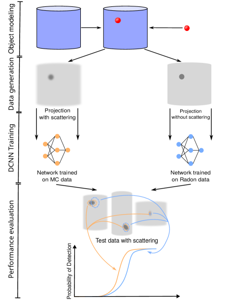
Figure 2: Application-driven approach to evaluate the difference between simulation with and without scattering. First, a large number of 3D volumes is created by combining different variations of object and defect geometry. Two forward projection methods are used to transform 3D volumes into X-ray projections. Each dataset containing a variety of projections is used to train a DCNN. They are applied to the same collection of test data with scattering. The performance of DCNNs is evaluated with POD curves.

3.1 Object modeling

Studying the influence of scattering poses multiple constraints for the data generation approach. In our methodology, we want to avoid cases when a DCNN fails to detect a defect because it was not exposed to a certain morphology during training. For example, if a network was trained on detecting defects in large objects, it might fail on a test projection with a small object regardless of scattering. In a perfect scenario, objects used for both the training and test sets should correspond to the same distribution of objects, and as many objects as possible should be in both sets. In real-world applications, test objects are measured experimentally, while the training objects are created digitally. Thus, it is difficult to guarantee that the distributions of training and test objects match.

We address these constraints by choosing to work with a model problem. Every 3D volume is created by combining a small number of objects following a parameterizable algorithm. Training and test sets of volumes are created with different random sequences of parameters, every parameter has the same distribution for both sets. Other than geometry, the volume is characterized by material properties. To consider a variety of scattering patterns, we repeat the experiments with the same geometry and different material composition.

The model problem we use in this study is the detection of cavities in cylinders. The object is a homogeneous cylinder parameterized by radius and height. The defect is an ellipsoidal void inside the cylinder. It is defined by ellipsoidal axes, height, and distance from the rotational axis of the cylinder. Materials of the cylinder are chosen from the common materials of industrial products: PMMA (type of plastic, synthetic polymer $(C_{5}O_{2}H_{8})_{n}$), aluminum, and iron.

3.2 Data generation

To make sure that the scattering distribution in the generated data is accurate and similar to real measurements, we choose to use Monte-Carlo simulation, specifically GATE (Jan et al., 2011). An accurate Monte-Carlo simulation requires a detailed knowledge of the experimental setup: X-ray source, studied object, and detector. However, not all of them are crucial for an accurate scattering simulation. The most important properties are the energy spectrum of emitted X-ray photons, attenuation curves of materials present in the object, and accurate description of the object geometry (defined as a voxelized volume, mesh, or a collection of simple shapes). GATE simulates every emitted photon individually and records its coordinates if it is registered by the detector.

The model problem simplifies defining object geometry and material composition. Object geometry is defined as a mix of a cylinder and an ellipsoid which are basic object shapes for GATE. Attenuation properties are computed automatically for a given chemical formula. We compute the X-ray source spectrum with an empirical model of an X-ray tube that provides an energy spectrum depending on the voltage. Multiple voltage values are selected for every material since scattering distribution heavily depends on both properties. We choose to perform a simulation with a perfect detector that registers every photon reaching it (technically implemented as a sufficiently thick layer of heavy material). Simulation of a realistic detector is possible with Monte-Carlo methods but is beyond the scope of this study. Such modeling would require detailed knowledge of a real detector that is often absent in industrial tasks.

The output of GATE includes the coordinates where every X-ray photon was detected and how many times it scattered before detection. By summing photons detected in every pixel of the detector, a total distribution of primary photons $P$ (Fig. 3a) and distribution of scattered photons $S$ (Fig. 3b) can be computed. Distribution of SPR is defined as $\frac{S}{P}$(Fig. 3c). Standard pre-processing consisting of flatfield correction and computing logarithm (according to Beer’s law) is used to make projections with and without the scattering signal (Figs. 3e and 3d).

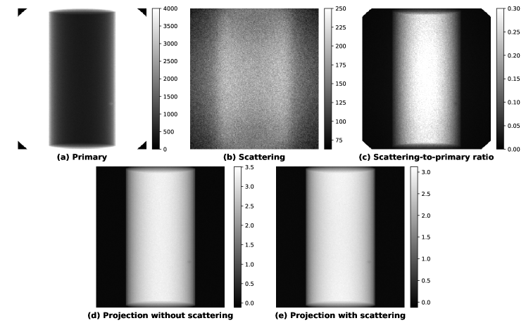
Figure 3: Different distributions of X-ray signal that are computed with a Monte-Carlo algorithm: distribution of primary photons registered by the detector (a), distribution of scattered photons (b), scattering-to-primary ratio (c), projection image without scattering after pre-processing (flatfield correction and logarithm according to Beer’s law) (d), projection image with scattering (e).

3.3 DCNN Training

As mentioned previously, defect detection can be performed in many ways. We focus on the defect detection via segmentation. This approach not only detects the presence of the defect but also provides its location on the projection. Training a segmentation DCNN requires a labeled dataset where every projection is accompanied by the ground-truth - a discrete image in which pixels corresponding to the defect are labeled accordingly. DCNN training is affected by random factors (initialization, GPU computations). Hence, every training is repeated multiple times to have multiple instances of the same DCNN. The performance of the instances is then averaged to determine the performance of the DCNN.

We choose the Mixed-Scale Dense convolutional neural network (MSD) (Pelt and Sethian, 2018) as the DCNN architecture (examples of results with different architectures are given in the Appendix). Due to dense connections and a small number of parameters, an MSD network can be trained quickly and provide accurate segmentations. To construct the ground-truth, the Radon transform is applied to 3D volumes, and the defect location corresponds to its projection. The DCNN trained on projections that include scattered photons will be referred to as the network trained on MC data. The one trained on data without the scattering signal will be referred to as the network trained on Radon data.

3.4 Performance evaluation

Many metrics can be applied to evaluate the similarity between the output of the segmentation DCNN and the ground-truth. In this study, we use $F_{1}$ score (equivalent to Dice’s coefficient) that can be computed according to the equation

$$F_{1}=\frac{2TP}{2TP+FP+FN}$$ (1)

where TP (True Positive) is the number of defect pixels that were segmented correctly, FP (False Positive) is the number of pixels that were incorrectly marked as corresponding to the defect, and FN (False Negative) denotes the number of defect pixels that were missed by a segmentation algorithm.

The $F_{1}$ score evaluates the accuracy of a DCNN for a single test case. A test dataset consists of many projections and requires another accuracy metric that combines all individual performance levels. A trivial solution would be to compute a mean accuracy on all projections in the dataset. This approach breaks when the variance of accuracies is too high: some projections are segmented almost perfectly while in others the defect is missed. Such behavior is easy to achieve with a wide range of objects and defects in the test set. Missing a defect does not necessarily mean that the DCNN is insufficiently accurate because features can be missed due to the imaging resolution and the noise level.

To study a DCNN performance on a varied test dataset, we follow the Probability of Detection (POD) analysis that is widely used for non-destructive testing (Georgiou, 2007) and was recently applied to X-ray CT (Tyystjärvi et al., 2022; Yosifov et al., 2022). We assume that segmentation accuracy depends on the defect size. By size, we refer to the largest intersection between the defect and primary X-ray trajectories (the largest thickness). This is not the only way to characterize the defect. For example, its area or perimeter can also be used to represent size. It is also important to mention that these properties are often correlated since the expected defects have similar shapes. Fig. 4a illustrates that $F_{1}$ significantly varies between different test cases with different defect sizes. Following POD methodology, we convert segmentation accuracy to a binary variable by defining segmentation as successful if $F_{1}>50\%$. This is an arbitrary choice that varies depending on the task. In Fig. 4b projections are divided into groups by binning defect size and a fraction of successful segmentations is computed for every bin. Segmentation accuracy gets better when the defect is larger.

The POD curve provides a continuous dependency of segmentation success rate on defect size by performing a log-likelihood fit. It is assumed that a segmentation is successful ($F_{1}>50\%$) with a probability $p$ that depends on the defect size $s$ according to

$$g(p)=\ln\frac{p}{1-p}=\alpha+\beta s,$$ (2)

where $\alpha$ and $\beta$ are fit parameters of a generalized linear model (GLM). The choice of logit function $g(p)$ is arbitrary, it can be replaced with other link functions such as log-log, complementary log-log, probit, etc. An example of a POD curve is shown in Fig. 4c. Since $\alpha$ and $\beta$ are results of the fit, their values have an uncertainty that can be described with a covariance matrix. Consequently, a confidence interval (95% confidence) can be drawn around the POD curve to indicate fit uncertainty.

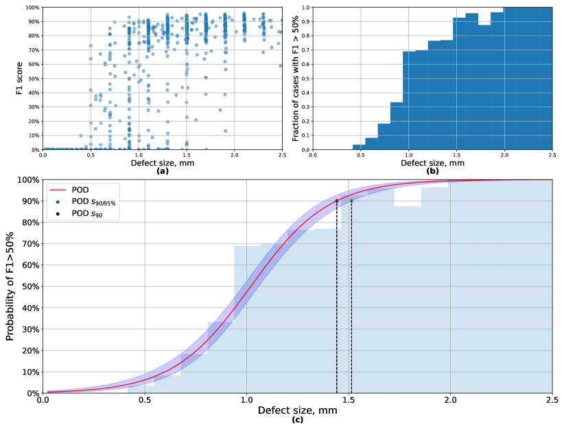
Figure 4: Example of a POD curve and its relation to the accuracy for a single projection: (a) the correlation between $F_{1}$ score and defect size for all projections in the test set, (b) a histogram computed after binning defect size indicating that the fraction of projections with $F_{1}>50\%$ increases with defect size, (c) the POD curve representing a probability of $F_{1}>50\%$ with highlighted smallest detectable defect $s_{90}$ and its lower bound.

In the POD curve applications, the value of $p=90\%$ is often computed as the smallest detectable defect. We will refer to this value as the $s_{90}$ - threshold for the defect size when the segmentation accuracy $F_{1}$ is higher than 50% with 90% probability. As every probability value has a lower and upper bound due to fit uncertainty, a lower bound for $s_{90}$ can also be defined as $s_{90/95}$. We will use both values to compare the performance of different DCNNs when tested on the same data.

The POD curve can be computed as a function of multiple variables, not only the defect size. For example, a defect location can be added as the second variable (Chen et al., 2021a). In the last subsection of Results, we study the dependency of POD on SPR by fitting

$$g(p)=\ln\frac{p}{1-p}=\alpha+\beta s+\gamma SPR.$$ (3)

If a certain parameter of the data heavily influences segmentation and is not included in the univariate fit, it will be effectively averaged to make a single curve. Multivariate fit mitigates this issue and allows studying the dependency explicitly.

4 Results

4.1 Software implementation

X-ray source spectra and material attenuation curves are generated using xpecgen (Hernández and Fernández, 2016). Monte-Carlo simulation for X-ray CT imaging is performed using GATE (Jan et al., 2011). PyTorch implementation of the MSD network is used for training and testing. POD curves are fitted with statsmodels package (Seabold and Perktold, 2010).

4.2 Generated data

Geometrical properties of the objects for the training and test sets are generated in advance and kept the same for all materials and voltages. We generate 1250 objects for the training set (1000 for training, 250 for validation) and 1000 objects for the test set. The radius of the cylinder varies from 1 to 25 mm, and height changes from 20 to 55 mm. Ellipsoidal cavities are generated as deformed spheres: first, a radius is chosen such that it lies in the range from 0.1 mm to 1 mm, and then the ratio between each axis and this radius lies in the range from 0.7 to 1.3. A cavity can be placed at any distance from the axis of rotation. The acquisition geometry stays the same for all datasets. The source-object distance (SOD) is 200 mm, and the source-detector distance (SDD) is 300 mm which leads to a magnification factor of 1.5. The detector plane is a 75$\times$ 82.5 $\textrm{mm}^{2}$ rectangle with a pixel size of 0.3 mm. Thus, generated projections have a size of 250 $\times$ 275 $\textrm{px}^{2}$. One projection contains MC simulations of $10^{9}$ emitted photons. Examples of these projections are shown in Fig. 5.

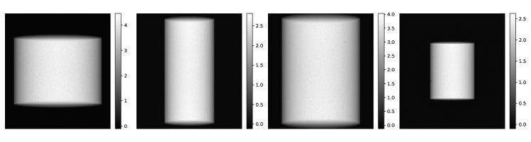
Figure 5: Examples of projections corresponding to different generated volumes.

Different material compositions and voltages are used to explore a variety of scattering distributions. In practice, heavier materials are inspected with higher voltage. Otherwise, only a small fraction of the X-ray radiation penetrates the object leading to a high noise level. The combination of material and voltage can be characterized by the value of HVL (Half-Value Layer) - the thickness of the object at which the intensity of X-ray entering it is reduced by one-half. PMMA is simulated with 90 kV (HVL = 27.8 mm) and 150 kV (HVL = 31.7 mm). Aluminum is simulated at 90 kV (HVL = 4.28 mm), 150 kV (HVL = 6.25 mm) and 300 kV (HVL = 17.9 mm). Iron is simulated at 300 kV (HVL = 3.85 mm) and 450 kV (HVL = 4.6 mm). Fig. 6 shows different scattering distributions for the same object depending on the material and voltage. The number of scattered photons (not necessarily SPR) increases with higher voltages and lower atomic numbers. Furthermore, there is a qualitative change in spatial properties: for materials with low atomic number scattering is more uniform, and for heavier materials it follows the shape of the object. This can be explained by different ratios of Rayleigh and Compton scattering and probabilities of further absorption in the object for scattered photons.

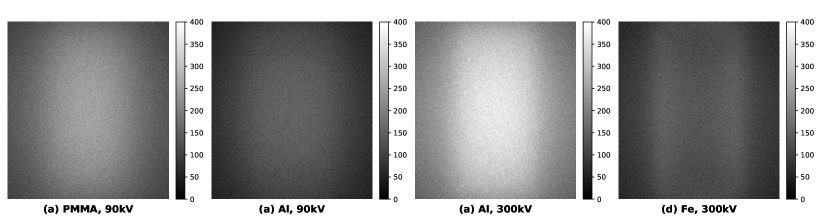
Figure 6: Comparison of scattering distributions for the same object made of different materials and inspected with different voltages of the tube: (a) PMMA at 90 kV, (b) aluminum at 90 kV, (c) aluminum at 300 kV, (d) iron at 300 kV. For the same voltage, the number of scattered photons is higher for materials with lower atomic number. For the same material, the amount of scattering is higher for higher voltage. Iron objects have a different scattering pattern with more photons close to the boundary.

4.3 Comparison of DCNN performance

For every combination of material and voltage, two DCNNs with the same architecture are trained on data without scattering (Radon data) and with scattering (MC data), 10 instances each. As explained in the Methods section, averaging the segmentation accuracy of the DCNN on the test dataset does not lead to a good performance estimate due to high variance. For example, in the case of iron at 450 kV the network trained on Radon data has a segmentation accuracy of 43% $\pm$ 40% on the test dataset while the network trained on MC data achieves 44% $\pm$ 40%. High variance is observed for every dataset and makes direct comparison of the DCNNs impossible.

For a detailed analysis of performance, POD curves are computed for both DCNNs for every combination of voltage and material. Fig. 7a shows a pair of POD curves for PMMA at 90 kV with no difference in performance between the networks trained on Radon and MC data. The POD curve for the Radon data network lies inside the 95% confidence interval of the MC POD curve which makes the difference between them statistically insignificant. The opposite case is shown for iron at 450 kV (Fig. 7c) where higher POD values for the network trained on Radon data lie below the confidence interval for the network trained on MC data (in particular, $s_{90}$). Hence, there is a statistically significant difference between training sets, and MC data lead to better performance. Nevertheless, the difference between $s_{90}$ is only 5% for iron at 450 kV and smaller for other datasets (e.g. for aluminum at 150 kV as shown in Fig. 7b). Furthermore, for defects larger than $s_{90}$, the mean segmentation accuracy is 82%$\pm$16% for the network trained on MC data and 82%$\pm$18% for the network trained on Radon data. Even though the variance is smaller than for the whole dataset, the performance of the two networks is still effectively the same.

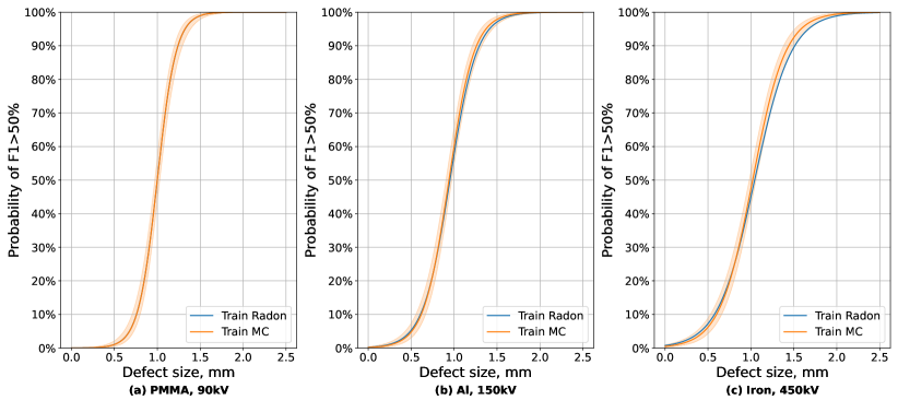
Figure 7: Comparison of POD curves for different datasets: (a) PMMA at 90 kV, (b) aluminum at 150 kV, (c) iron at 450 kV. The difference between training on projections with and without scattering is negligible for PMMA. It becomes larger for aluminum but within a 95% confidence interval. For iron at 450 kV, the network trained on MC data performs better than the network trained on Radon data taking into account the confidence interval.

Values of $s_{90}$ for both networks in all cases are shown in Table 1. In most cases (except for iron at 450 kV) the difference in the smallest segmentable defect between networks is smaller than the confidence interval. This serves as an upper estimate for the possible difference in performance. Depending on the material and voltage, the relative difference in $s_{90}$ stays between 0% and 3% and is unlikely to exceed 5% even if the fit coefficients are not determined precisely.

Material, kV	MC data net, s90 [mm]	MC data net, s90/95 [mm]	Radon data net, s90 [mm]	s90 difference
PMMA, 90 kV	1.24	1.29	1.24	0%
PMMA, 150 kV	1.31	1.36	1.31	0.2%
Al, 90 kV	1.39	1.46	1.42	1.9%
Al, 150 kV	1.26	1.32	1.29	2.4%
Al, 300 kV	1.17	1.22	1.18	0.8%
Iron, 300 kV	1.59	1.68	1.62	1.7%
Iron, 450 kV	1.44	1.51	1.51	5.0%

Table 1: Smallest detectable defect size for different materials and training datasets.

4.4 Influence of scattering-to-primary ratio

The negligible difference in the performance of the networks trained on Radon and MC data raises the question of biases in test data and projection properties that influence segmentation. For every dataset, we perform a multivariate POD fit following Eq. 3 to evaluate the influence of SPR at the defect location. After determining POD coefficients, the value of SPR can be fixed at a certain level to obtain POD for this amount of scattering signal (Fig. 8 for PMMA, aluminum, and iron).

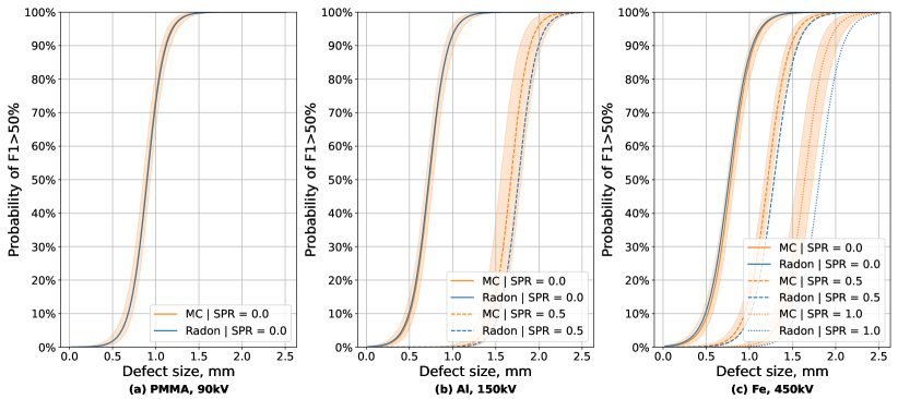
Figure 8: Comparison of multivariate POD curves computed at different values of SPR for different datasets: PMMA at 90 kV (a), aluminum at 150 kV (b), and iron at 450 kV (c). Increasing SPR leads to a larger difference between the POD curves of the networks trained on Radon and MC data. Pairs of POD curves are plotted for SPR values of 0., 0.5, and 1.0 if such projections are present in the dataset (the largest SPR for PMMA is 0.16, for aluminum it is 0.55).

Several observations can be made after splitting the dataset based on the SPR value. First, with higher SPR the difference between the networks trained on Radon and MC data increases. This can be determined by either performing a multivariate fit or making a univariate fit for a subset of test data (with a sufficiently high SPR). Second, the values of $s_{90}$ increase for higher SPR. Third, different datasets have different distributions of SPR. For example, aluminum at 150 kV has 500 objects with SPR $<0.1$ while iron at 450 kV has 400 such objects. Hence, even if in both cases there is no difference between the networks trained on Radon and MC data for low SPR, the overall POD curve are more affected by this for aluminum since such cases are more frequent.

It is important to note that POD curves only indicate a correlation between the DCNN accuracy and the different properties of the projection. Furthermore, the value of SPR at the defect location is correlated with other properties, such as attenuation rate as shown in Fig. 9. The attenuation rate $\mu$ in a pixel is computed as $-\log\frac{I}{I_{0}}$ where $I_{0}$ is the total number of photons emitted in the direction of the pixel and $I$ is the number of registered photons (including scattered radiation). Noise in the MC simulation follows a Poisson distribution and depends on $I$. Regions with high SPR often have high $\mu$ which leads to high relative noise levels. This correlation could explain the increase in $s_{90}$ for higher SPR.

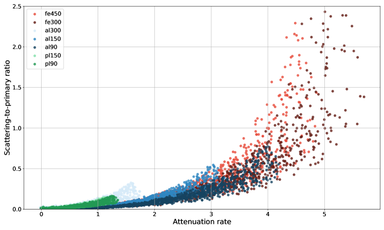
Figure 9: Correlation between projection properties at the defect location (SPR and attenuation rate) for different datasets (markers are colored with shades of red for iron, blue for aluminum, and green for PMMA). SPR increases with the attenuation rate, and the dependency might be similar for datasets with different materials and voltages.

In Table 2 we compare $s_{90}$ values in every dataset at the minimum and maximum SPR levels (minimum is almost 0 in each case). With the sole exception of PMMA at 90 kV (where it can be explained by fit uncertainty), higher SPR leads to a larger difference in performance between the networks trained on Radon and MC data. The geometrical structure of the test dataset leads to a large number (around 40-50%) of cases with low SPR, mostly due to the small size of the object. In these cases, there is little difference between training on data with and without scattering. Consequently, the performance on the whole test dataset becomes more similar even if in other cases the MC network has a smaller $s_{90}$.

Material, kV	Max SPR	At SPR = 0		At Max SPR
		MC, $s_{90}$	Radon, $s_{90}$	MC, $s_{90}$	Radon, $s_{90}$
PMMA, 90 kV	0.16	1.11	1.12	1.59	1.57
PMMA, 150 kV	0.14	1.22	1.19	1.57	1.63
Al, 90 kV	0.77	1.00	0.97	2.38	2.51
Al, 150 kV	0.55	0.96	0.96	1.99	2.09
Al, 300 kV	0.33	1.07	1.07	1.47	1.50
Fe, 300 kV	5.26	1.02	1.03	5.84	6.06
Fe, 450 kV	2.29	1.05	1.04	3.02	3.44

Table 2: Difference in $s_{90}$ for minimal and maximal SPR values

5 Discussion

We presented a methodology that evaluates the difference between training data for DCNNs using a model problem as an example. This methodology can be applied to various defect detection tasks, as individual parts of the methodology can be replaced to better fit a particular problem. The core components are the training data both including and excluding X-ray scattering signal, test data including scattering signal, and an algorithm that extracts prior information from the training data and can be applied to the test data (e.g. machine learning or deep learning method). POD curves can be used to evaluate the accuracy of any algorithm that takes a test projection as an input including inspection by a human expert.

In the presented model problem, both training and test data are generated with a Monte-Carlo algorithm. This approach provides an easy way to get two versions of the same data that only differ by the presence of scattering. Alternatively, the same result can be achieved with the real data and either software or hardware scattering reduction techniques to get projections without the scattering signal. The biggest disadvantage of using experimental data is that scattering would only be approximately removed while Monte-Carlo simulation can ensure that no scattering is present in the data. Furthermore, GATE and GEANT4 are verified to produce highly accurate results with sufficient computational time. The biggest drawback of our implementation of the MC simulation is the lack of the detector response that would be present in the real data. Said drawback is partially mitigated by the level of stochastic noise.

We performed defect detection using MSD architecture for a segmentation DCNN. In the Appendix, we show that similar results can be achieved with other DCNN architectures, including DeepLabv3, UNet++, and FPN. We have tried to train a classification network instead of segmentation but the results were inferior. Such difference in performance can be explained by the lack of the defect mask in the training data that complicates the learning process. Using deep learning is not necessary for the presented methodology. A machine learning algorithm with manually defined features that extracts thresholds from the training data can be used too. POD curves are applicable to any image processing algorithm and only require a single value of a previously defined metric for every test projection. The biggest drawback of POD curves is that they only find correlations in the data and cannot prove that a change in performance is caused by differences in the training data. The threshold of 50% $F_{1}$ score to convert network accuracy into a binary variable is chosen arbitrarily. If increased, it will shift POD curves to the right with respect to the defect size.

While the presented results are only valid for a chosen problem, they illustrate the advantages of using a POD-based methodology. A significant difference in accuracy was only present in a small subset of test projections, and this effect was not visible for other metrics due to variance. Furthermore, POD curves address a concept of the smallest detectable defect that helps to evaluate if a system is useful for a particular real-world application. We expect a similar effect of scattering on inspection performance in other problems too. If a defect is too small, the contrast in X-ray attenuation is lower than the noise level, and the inclusion of scattering does not significantly affect the detection process. If a defect is too large, the contrast would be larger than a variance in signal due to scattering. Consequently, the biggest influence of scattering signal should be seen for barely detectable defects when the contrast is similar to the noise level.

It is important to note that any defect detection problem has a number of system properties that affect noise level and SPR and, consequently, the effect of excluding the scattering signal from the training data. The distance between the object and the detector (known in radiology as the air gap) significantly influences SPR values because scattered photons might not reach the detector. Furthermore, a smaller field of view and small objects can decrease the impact of the scattering signal. Higher exposure time decreases the noise level and $s_{90}$, so the effect of scattering as additional noise might become more significant.

6 Conclusion

The practical application of data generation techniques for defect detection in industrial products requires a balance between the computational cost of generation and the resulting accuracy of the algorithm. We have proposed a methodology to quantitatively evaluate the effect of simulating X-ray scattering on data generation for training DCNNs. The POD curves have been used to study the network performance in detail by correlating it with the properties of the test projections. Using a Monte-Carlo simulation algorithm, we have ensured that the difference between DCNNs was only caused by the presence of the scattering signal. Our performance analysis was successfully applied to the varied test cases. The POD curves have shown under which test conditions the difference between DCNNs is significant and when it is negligible. In particular, we have demonstrated how the scattering-to-primary ratio affected the network accuracy and the influence of the data generation approach. The presented methodology can be used to decide if the defect detection performance is sufficient for a particular task and what level of accuracy in data generation is necessary to achieve that performance.

CRediT authorship contribution statement

Vladyslav Andriiashen: Conceptualization, Methodology, Software, Validation, Formal analysis, Investigation, Resources, Data Curation, Writing - Original Draft, Writing - Review & Editing, Visualization. Robert van Liere: Conceptualization, Methodology, Writing - Review & Editing, Visualization, Supervision. Tristan van Leeuwen: Conceptualization, Methodology, Writing - Review & Editing, Resources, Supervision, Project administration. Kees Joost Batenburg: Writing - Review & Editing, Resources, Project administration.

Declaration of Competing Interest

The authors declare that they have no known competing financial interests or personal relationships that could have appeared to influence the work reported in this paper.

Code and Data availability

The code for Monte-Carlo simulations can be found on Github: https://github.com/vandriiashen/mc-scattering. The data for training and testing were generated using this code. Sequences of parameters used for volume generation are included in the repository. Scripts for DCNN training and POD computation are in https://github.com/vandriiashen/pod-xray-images.

Appendix A Different DCNN architectures

For the dataset of iron at 450 kV we have trained DCNNs with different state-of-the-art architectures using the Segmentation Models package (Iakubovskii, 2019). We have tried UNet++, FPN (Feature Pyramid Network), and DeepLabv3+ as semantic segmentation architectures, and EfficientNet, MobileNet, and ResNet (not included in the results because the performance was significantly worse) as encoders. Then the accuracy of every network on the test dataset was evaluated with POD curves in the same way as for MSD (Fig. 10a). The networks have similar performance, the difference in $s_{90}$ between the best and the worst model is around 10%. The difference between training on Radon and MC data can be evaluated for other network architectures, and the effect is similar to MSD. For example, Fig. 10b is made with the same data as Fig. 7c, but the network architecture is DeepLabv3+ instead of MSD.

The similarity between network performance indicates that the difficulty of segmentation in the model problem stems from the image and noise properties and not from deep learning. This supports the assumption that the generated projections have enough variety for training a DCNN.

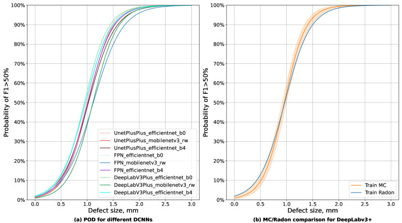
Figure 10: Comparison of POD curves for the DCNNs with different architectures tested on the dataset of iron at 450 kV. DeepLabv3+ outperforms other tested architectures, MSD achieves one of the highest accuracy levels despite the fewest number of parameters. The difference in $s_{90}$ is around 10% when comparing the best and the worst model (a). Comparison of the networks trained on MC and Radon data when the network uses DeepLabv3+ architecture with EfficientNetB0 encoder. The decrease in $s_{90}$ is similar to MSD (b).

References

- Agostinelli et al. (2003) Agostinelli, S., Allison, J., Amako, K.a., Apostolakis, J., Araujo, H., Arce, P., Asai, M., Axen, D., Banerjee, S., Barrand, G., et al., 2003. GEANT4 — a simulation toolkit. Nuclear instruments and methods in physics research section A: Accelerators, Spectrometers, Detectors and Associated Equipment 506, 250–303.
- Andriiashen et al. (2023) Andriiashen, V., van Liere, R., van Leeuwen, T., Batenburg, K.J., 2023. CT-based data generation for foreign object detection on a single x-ray projection. Scientific Reports 13, 1881.
- Armanious et al. (2020) Armanious, K., Jiang, C., Fischer, M., Küstner, T., Hepp, T., Nikolaou, K., Gatidis, S., Yang, B., 2020. MedGAN: Medical image translation using GANs. Computerized medical imaging and graphics 79, 101684.
- Aydin et al. (2018) Aydin, I., Karakose, M., Erhan, A., 2018. A new approach for baggage inspection by using deep convolutional neural networks, in: 2018 International Conference on Artificial Intelligence and Data Processing (IDAP), IEEE. pp. 1–6.
- Barnes (1991) Barnes, G.T., 1991. Contrast and scatter in x-ray imaging. Radiographics 11, 307–323.
- Bellon and Jaenisch (2007) Bellon, C., Jaenisch, G.R., 2007. aRTist–analytical RT inspection simulation tool, in: Proc DIR, pp. 25–27.
- Bhatia et al. (2016) Bhatia, N., Tisseur, D., Buyens, F., Létang, J.M., 2016. Scattering correction using continuously thickness-adapted kernels. NDT & E International 78, 52–60.
- Bian et al. (2016) Bian, X., Lim, S.N., Zhou, N., 2016. Multiscale fully convolutional network with application to industrial inspection, in: 2016 IEEE winter conference on applications of computer vision (WACV), IEEE. pp. 1–8.
- Cardoso et al. (2009) Cardoso, S., Gonçalves, O., Schechter, H., 2009. Evaluation of scatter-to-primary ratio in radiological conditions. Applied Radiation and Isotopes 67, 544–548.
- Chen et al. (2021a) Chen, G., Guo, Y., Katagiri, T., Song, H., Tomizawa, T., Yusa, N., Hashizume, H., 2021a. Multivariate probability of detection (pod) analysis considering the defect location for long-range, non-destructive pipe inspection using electromagnetic guided wave testing. NDT & E International 124, 102539.
- Chen et al. (2021b) Chen, H., Nie, X., Gan, S., Zhao, Y., Qiu, H., 2021b. Interfacial imperfection detection for steel-concrete composite structures using ndt techniques: A state-of-the-art review. Engineering Structures 245, 112778.
- Cunha et al. (2010) Cunha, D., Tomal, A., Poletti, M.E., 2010. Evaluation of scatter-to-primary ratio, grid performance and normalized average glandular dose in mammography by Monte Carlo simulation including interference and energy broadening effects. Physics in Medicine & Biology 55, 4335.
- Georgiou (2007) Georgiou, G.A., 2007. PoD curves, their derivation, applications and limitations. Insight-Non-Destructive Testing and Condition Monitoring 49, 409–414.
- Gong et al. (2019) Gong, Q., Greenberg, J.A., Stoian, R.I., Coccarelli, D., Vera, E., Gehm, M.E., 2019. Rapid simulation of X-ray scatter measurements for threat detection via GPU-based ray-tracing. Nuclear Instruments and Methods in Physics Research Section B: Beam Interactions with Materials and Atoms 449, 86–93.
- Gong et al. (2018) Gong, Q., Stoian, R.I., Coccarelli, D.S., Greenberg, J.A., Vera, E., Gehm, M.E., 2018. Rapid simulation of X-ray transmission imaging for baggage inspection via GPU-based ray-tracing. Nuclear Instruments and Methods in Physics Research Section B: Beam Interactions with Materials and Atoms 415, 100–109.
- Hernández and Fernández (2016) Hernández, G., Fernández, F., 2016. xpecgen: A program to calculate x-ray spectra generated in tungsten anodes. J. Open Source Softw. 1, 62.
- Iakubovskii (2019) Iakubovskii, P., 2019. Segmentation Models Pytorch. https://github.com/qubvel/segmentation_models.pytorch.
- ISO 16371-2: (2017) ISO 16371-2:2017, 2017. Non-destructive testing — Industrial computed radiography with storage phosphor imaging plates — Part 2: General principles for testing of metallic materials using X-rays and gamma rays. Standard. International Organization for Standardization. Geneva, CH.
- Jan et al. (2011) Jan, S., Benoit, D., Becheva, E., Carlier, T., Cassol, F., Descourt, P., Frisson, T., Grevillot, L., Guigues, L., Maigne, L., et al., 2011. GATE v6: a major enhancement of the gate simulation platform enabling modelling of ct and radiotherapy. Physics in Medicine & Biology 56, 881.
- Lee et al. (2021) Lee, K., Yi, S., Hyun, S., Kim, C., 2021. Review on the recent welding research with application of CNN-based deep learning part I: Models and applications. Journal of Welding and Joining 39, 10–19.
- Maier et al. (2018) Maier, J., Sawall, S., Knaup, M., Kachelrieß, M., 2018. Deep scatter estimation (DSE): Accurate real-time scatter estimation for X-ray CT using a deep convolutional neural network. Journal of Nondestructive Evaluation 37, 1–9.
- Masci et al. (2012) Masci, J., Meier, U., Ciresan, D., Schmidhuber, J., Fricout, G., 2012. Steel defect classification with max-pooling convolutional neural networks, in: The 2012 international joint conference on neural networks (IJCNN), IEEE. pp. 1–6.
- Mery (2015) Mery, D., 2015. Computer vision for X-Ray testing. Switzerland: Springer International Publishing 10, 978–3.
- Mery et al. (2015) Mery, D., Riffo, V., Zscherpel, U., Mondragón, G., Lillo, I., Zuccar, I., Lobel, H., Carrasco, M., 2015. GDXray: The database of X-ray images for nondestructive testing. Journal of Nondestructive Evaluation 34, 1–12.
- Parlak and Emel (2023) Parlak, İ.E., Emel, E., 2023. Deep learning-based detection of aluminum casting defects and their types. Engineering Applications of Artificial Intelligence 118, 105636.
- Pelt and Sethian (2018) Pelt, D.M., Sethian, J.A., 2018. A mixed-scale dense convolutional neural network for image analysis. Proceedings of the National Academy of Sciences 115, 254–259.
- Rührnschopf and Klingenbeck (2011) Rührnschopf, E.P., Klingenbeck, K., 2011. A general framework and review of scatter correction methods in x-ray cone-beam computerized tomography. part 1: scatter compensation approaches. Medical physics 38, 4296–4311.
- Seabold and Perktold (2010) Seabold, S., Perktold, J., 2010. statsmodels: Econometric and statistical modeling with python, in: 9th Python in Science Conference.
- Sun and Star-Lack (2010) Sun, M., Star-Lack, J., 2010. Improved scatter correction using adaptive scatter kernel superposition. Physics in Medicine & Biology 55, 6695.
- Tempelaere et al. (2023) Tempelaere, A., Van De Looverbosch, T., Kelchtermans, K., Verboven, P., Tuytelaars, T., Nicolai, B., 2023. Synthetic data for X-ray CT of healthy and disordered pear fruit using deep learning. Postharvest Biology and Technology 200, 112342.
- Tyystjärvi et al. (2022) Tyystjärvi, T., Virkkunen, I., Fridolf, P., Rosell, A., Barsoum, Z., 2022. Automated defect detection in digital radiography of aerospace welds using deep learning. Welding in the World 66, 643–671.
- Van De Looverbosch et al. (2022) Van De Looverbosch, T., He, J., Tempelaere, A., Kelchtermans, K., Verboven, P., Tuytelaars, T., Sijbers, J., Nicolai, B., 2022. Inline nondestructive internal disorder detection in pear fruit using explainable deep anomaly detection on X-ray images. Computers and Electronics in Agriculture 197, 106962.
- Yang et al. (2020) Yang, J., Li, S., Wang, Z., Dong, H., Wang, J., Tang, S., 2020. Using deep learning to detect defects in manufacturing: a comprehensive survey and current challenges. Materials 13, 5755.
- Yosifov et al. (2022) Yosifov, M., Reiter, M., Heupl, S., Gusenbauer, C., Fröhler, B., Fernández-Gutiérrez, R., De Beenhouwer, J., Sijbers, J., Kastner, J., Heinzl, C., 2022. Probability of detection applied to x-ray inspection using numerical simulations. Nondestructive Testing and Evaluation 37, 536–551.