On the isotropy of SnIa absolute magnitudes in the Pantheon+ and SH0ES samples

Abstract

We use the hemisphere comparison method to test the isotropy of the SnIa absolute magnitudes of the Pantheon+ and SH0ES samples in various redshift/distance bins. We compare the identified levels of anisotropy in each bin with Monte-Carlo simulations of corresponding isotropised data to estimate the frequency of such levels of anisotropy in the context of an underlying isotropic cosmological. We find that the identified levels of anisotropy in all bins are consistent with the Monte-Carlo isotropic simulated samples. However, in the real samples for both the Pantheon+ and the SH0ES cases we find sharp changes of the level of anisotropy occuring at distances less than $40Mpc$. For the Pantheon+ sample we find that the redshift bin $[0.005,0.01]$ is significantly more anisotropic than the other 5 redshift bins considered. For the SH0ES sample we find a sharp drop of the anisotropy level at distances larger than about $30Mpc$. These anisotropy transitions are relatively rare in the Monte-Carlo isotropic simulated data and occur in $2\%$ of the SH0ES simulated data and at about $7\%$ of the Pantheon+ isotropic simulated samples. This effect is consistent with the experience of an off center observer in a $30Mpc$ bubble of distinct physics or systematics.

I Introduction

The cosmological principle (CP)Aluri et al. (2023) is a cornerstone of the standard cosmological model $\Lambda$CDM . It assumes that the Universe is homogeneous and isotropic on scales larger than about $100Mpc$. This assumption is consistent with most cosmological observations and allows the use of the FRW metric as a background where cosmological perturbation grow to form the observed large scale structure. The main cosmological observation that supports the CP is the isotropy of the Cosmic Microwave Background (CMB) and observations of the distribution of galaxies on scales larger than $100Mpc$ which are consistent with the onset of homogeneity and isotropy on these scales.

Despite of the simplicity and overall observational consistency of the CP, a few challenges have developed during the past several years which appear to consistently question the validity of the CP on cosmological scales larger than $100Mpc$ and motivate further tests to be imposed on its validity. Some of these challenges pointing to preferred directions on large cosmological scales include the quasar dipoleSecrest et al. (2021); Zhao and Xia (2021); Hu et al. (2020); Guandalin et al. (2022); Dam et al. (2022), the radio galaxy dipoleWagenveld et al. (2023); Qiang et al. (2020); Singal (2023), the bulk velocity flowWatkins et al. (2023); Watkins and Feldman (2015); Wiltshire et al. (2013); Nadolny et al. (2021), the dark velocity flowAtrio-Barandela et al. (2015), the CMB anomaliesCopi et al. (2010); Schwarz et al. (2016), the galaxy spin alignmentTempel and Libeskind (2013); Simonte et al. (2023); Shamir (2022), the galaxy cluster anisotropies Bengaly et al. (2017), and a possible SnIa dipoleSorrenti et al. (2022); McConville and Colgáin (2023). These observational challenges of the CP may be indirectly connected with other tensions of the standard $\Lambda$CDM model including the Hubble Perivolaropoulos and Skara (2022a); Peebles (2022); Abdalla et al. (2022) and growth tensions Heymans et al. (2021); Troxel et al. (2018); Asgari et al. (2020); van Uitert et al. (2018) where the best fit parameter values of the model $H_{0}$ and $\sigma_{8}$ appear to be inconsistent when probed by different observational data. These tensions may indicate that a new degree of freedomSolà Peracaula et al. (2018); Anand et al. (2017); Di Valentino et al. (2021, 2017); Wang (2020); Gómez-Valent and Solà (2017); Di Valentino and Bridle (2018) is required to be introduced in the $\Lambda$CDM model. For example it would be in principle possible that these tensions may disappear if the new degree of freedom corresponding to anisotropy was allowed to be introduced in the data analysisTsagas (2022); Asvesta et al. (2022); Tsagas (2021, 2010); Colgáin (2019); Krishnan et al. (2021); McConville and Colgáin (2023).

An efficient method to test the CP is the use of type Ia supernovae (SnIa) which can map the expansion rate of the Universe up to redshifts of about 2.5. The latest and most extensive SnIa sample is the Pantheon+ sampleBrout et al. (2022a); Scolnic et al. (2022); Brout et al. (2022b).It provides equatorial coordinates, apparent magnitudes, distance moduli and other SnIa properties, derived from 1701 light curves of 1550 SnIa in a redshift range $z\in[0.001,2.26]$ compiled across 18 different surveys. This sample is significantly improved over the first Pantheon sample of 1048 SnIa Scolnic et al. (2018), particularly at low redshifts $z$.

The Pantheon+ sample has been used extensively for testing cosmological models and fitting cosmic expansion history parametrizations of $H(z)$ Brout et al. (2022a). It has also been used to identify and constrain possible velocity dipoles and compare with the corresponding velocity dipole obtained from the CMB. It was found that even though the observer velocity amplitude agrees with the dipole found in the cosmic microwave background, its direction is different at high significanceSorrenti et al. (2022). These results are in some tension with previous studies based on the previous Pantheon sampleHorstmann et al. (2022). The isotropy of $H_{0}$ has also been investigated using the hemisphere comparizon method Zhai and Percival (2022); McConville and Colgáin (2023); Krishnan et al. (2022a, 2021, b); Luongo et al. (2022); Zhai and Percival (2023) and relatively small but statistically significant anisotropy level was identified in the direction of the CMB dipole. Since there is degeneracy between $H_{0}$ and the SnIa absolute magnitude a possible anisotropy in the best fit value of $H_{0}$ is probably connected with an anisotropy of the SnIa absolute magnitudes.

Recent analyses have pointed out that a sudden change (transition) of the SnIa absolute magnitude by about $0.2$ at a transition redshift $z\lesssim 0.01$ could imply a lower value of $H_{0}$ compared to the one measured in the context of a standard distance ladder approach that does not incorporate this transition degree of freedom Marra and Perivolaropoulos (2021); Alestas et al. (2021a); Perivolaropoulos and Skara (2022a, b). Such a sudden change could occur in the context of a gravitational physics transition taking place globally during the past 150 Myrs, or locally in a bubble of scale of about $40Mpc$ and shifting the strength of gravity by a few percent. Such a transition would lead to a systematic dimming of SnIa which could be incorrectly interpreted as a higher value of $H_{0}$ due to the degeneracy between $H_{0}$ and $M$. It has recently been shown that such a scenario is consistentPerivolaropoulos and Skara (2022b) with the SH0ES dataRiess et al. (2022), with the Pantheon+ dataPerivolaropoulos and Skara (2023) and with other astrophysical and geological observationsAlestas et al. (2021b); Perivolaropoulos (2022).

This scenario may be realized in the context of a local $40Mpc$ bubble rather than a global transition at late times. In this case an off-center observer would detect a sudden increase of the anisotropy of the SnIa absolute magnitudes in spherical distance bins that include parts of both the inside and the outside region of the transition bubble (intermediate anisotropic distance bin in Fig. 1). Distance bins that are much larger of much smaller than the radius of the transition bubble would appear isotropic to the off center observer as shown in Fig. 1.

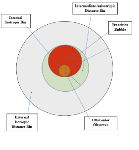
Figure 1: Demonstration of the predicted change of the anisotropy level of SnIa absolute magnitudes experienced by an off-center observer (center of small pink circle) in a gravitational transition bubble (red circle) where the gravitational constant is different by a few percent. A low anisotropy is expected in the small pink distance bin, a large anisotropy level is expected for the distance bin between the pink inner circle and the green outer circle and finally a smaller anisotropy level is expected for the distance bin between the green and the grey outer circles.

In the context of this prediction of the transition model for the anisotropy of the SnIa absolute magnitudes, the following questions arise:

• What is an efficient and general purpose statistic to quantitatively describe the anisotropy level of the SnIa absolute magnitudes of the Pantheon+ sample?

• Given such a statistic, what is the level of anisotropy of the SnIa absolute magnitudes for various distance (redshift) bins of the Patheon+ and SH0ES samples?

• What are the directions corresponding to these anisotropies for each redshift bin and how do these directions relate to the CMB dipole?

• What are the corresponding results expected in the context of Monte-Carlo simulated data of Pantheon+ in the context of isotropy?

• Are the above answers for the Pantheon+ and SH0ES samples consistent with each other?

The goal of the present analysis is to address these questions. In order to address these questions we obtain the SnIa absolute magnitudes as

$$M=m_{B}-\mu$$ (1)

where $m_{B}$ is the apparent magnitude of SnIa and $\mu$ is the distance modulus obtained either from the Cepheids co-hosted with the SnIa (published with the Pantheon+ data) or from the best fit $\Lambda$CDM model as obtained from Pantheon+.

The structure of this paper is the following: In the next section II we describe the statistic $\Sigma_{max}$ used to quantify the anisotropy level in our analysis and the hemisphere comparison method implemented in the context of this statistic. The implementation of this method is presented in section III for both the Pantheon+ and the SH0ES samples. The results of this anisotropy analysis are presented and qualitatively compared with those expected in the context of the local transition model predictions. Finally in section IV we summarize our main results, discuss their implications and describe possible future extensions of this analysis.

II The hemisphere comparison method

The hemisphere comparison methodSchwarz and Weinhorst (2007); Antoniou and Perivolaropoulos (2010) along with the dipole method has been extensively usedMariano and Perivolaropoulos (2013, 2012); Deng and Wei (2018a); Chang and Lin (2015); Kazantzidis and Perivolaropoulos (2020); Deng and Wei (2018b) for the identification of the level of anisotropy and the corresponding direction in a wide range of cosmological data. The implementation of this method in the present analysis involves the following steps:

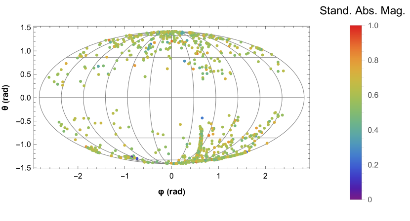
Figure 2: Mollweide projection in the galactic frame of the sky distribution of the Pantheon+ SnIa. Both angular coordinates are in radians and the azimouthal coordinate ranges in the projected range of $[-\pi,\pi]$ The color describes the SnIa standardized absolute magnitudes $\bar{M}$.

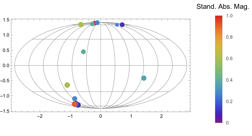
(a) The SnIa distribution in the lowest redshift bin $[0.001,0.005]$. The color denotes the standardized absolute magnitude $\bar{M}$ and the radius of each point increases with redshift. There are 29 SnIa but not all of them are shown due to overlap of directions since in this distance range there are SnIa that share the same host and thus the same galactic coordinates.

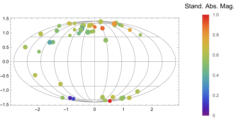
(b) The SnIa distribution in the redshift bin $[0.005,0.01]$.

Figure 3: The SnIa sky distribution in the two lowest redshift bins.

• Use the publicly available Pantheon+ dataBrout et al. (2022a) to estimate the absolute magnitude of each one of the 1701 SnIa using eq, (1) where $\mu$ is obtained from the Cepheid estimate for SnIa in Cepheid hosts or from the best fit Pantheon+ $\Lambda$CDM model with $\Omega_{0m}=0.333$, $h=0.734$ for the rest of the SnIaBrout et al. (2022a); Perivolaropoulos and Skara (2023). For these SnIa we set

  $$\mu(z)=5\;log_{10}(d_{L}(z;\Omega_{0m},h)/Mpc)+25$$ (2)

  where

  $$d_{L}(z;\Omega_{0m},h)=c(1+z)\int_{0}^{z}\frac{dz^{\prime}}{H(z^{\prime};\Omega_{0m},h)}$$ (3)

  is the luminosity distance and

  $$H(z)=100\;h\left[\Omega_{0m}(1+z)^{2}+(1-\Omega_{0m})\right]^{1/2}$$ (4)

  is the Hubble expansion rate for $\Lambda$CDM ($H_{0}=100\;h\;km/sec\cdot Mpc$). The residual absolute magnitude may be defined as

  $$M_{res}\equiv M_{i}-M_{SH0ES}$$ (5)

  where $M_{SH0ES}=-19.2483$ is the best fit SnIa absolute magnitude as obtained from the SH0ES dataRiess et al. (2022). In what follows, we use the residual absolute magnitudes $M_{res}$ but omit the index _res for simplicity. The uncertainty of each (residual) $M$ may be estimated using the uncertainties of $m$ and $\mu$ from eq. (1) as

  $$\sigma_{M}=\sqrt{\sigma_{m}^{2}+\sigma_{\mu}^{2}}$$ (6)

  where $\sigma_{m}$ and $\sigma_{\mu}$ are uncertainties of the apparent magnitude and the distance modulus as provided by the Pantheon+ sample. The mean of these residual absolute magnitudes is 0. For plotting convenience we also use the standardized absolute magnitudes defined as

  $${\bar{M}}\equiv\frac{M-M_{min}}{M_{max}-M_{min}}$$ (7)

  where $M_{max}$, $M_{min}$ are the maximum and minimum values of the SnIa absolute magnitudes. Obviously by definition ${\bar{M}}\in[0,1]$.

• The published SnIa coordinates of SnIa in Pantheon+ are equatorial coordinates (RA,DEC). We thus convert them to galactic coordinates $(l,b)$ using standard algorithmsDuffett-Smith and Zwart (2011). The resulting map of the SnIa absolute magnitudes is shown in Fig. 2. In Fig. 3 we also show the corresponding angular distribution for two redshift bins: $z\in[0.001,0.005]$ in Fig. 3(a) (29 points, some of them overlapping) and $z\in[0.005,0.01]$ in Fig. 3(b) (82 points). The color of the points denotes the standardized absolute magnitude while the radius of the points in Fig. 3 increases with the redshift.

• In a given redshift bin we consider a random direction in galactic coordinates and split the sample in two subsamples: one with SnIa in the ’North’ hemisphere with respect to this random direction and one in the ’South’ hemisphere. For each hemisphere we construct the weighted average (residual) absolute magnitude ($M_{N}$ and $M_{S}$) and the corresponding uncertainties ($\sigma_{N}$ and $\sigma_{S}$) using the equations

  $$M_{N}=\frac{\sum_{i}{M_{N,i}/\sigma_{N,i}^{2}}}{\sum_{i}{1/\sigma_{N,i}^{2}}}$$ (8)

  where the sum runs over the SnIa of the ’North’ hemisphere. Similarly we obtain $M_{S}$ for the ’South’ hemisphere with respect to the given random direction. The corresponding uncertainty of $M_{N}$ is obtained as

  $$\sigma_{N}=\sqrt{\left(\sum_{i}{1/\sigma_{N,i}^{2}}\right)^{-1}}$$ (9)

  and similarly for $\sigma_{S}$.

• We construct the statistical variable representing the anisotropy level for the given random direction

  $$\Sigma\equiv\frac{|M_{N}-M_{S}|}{\sqrt{\sigma_{N}^{2}+\sigma_{S}^{2}}}$$ (10)

• We evaluate $\Sigma$ for 1000 random directions and select the maximum anisotropy direction leading to the maximum anisotropy level $\Sigma_{max}$.

• We generate Monte-Carlo simulated versions of the Pantheon+ and SH0ES residual absolute magnitudes by replacing each SnIa absolute magnitude my a random value selected from a Gaussian distribution with 0 mean and standard deviation given by eq. (6) for each residual absolute magnitude $M$.

• For each one of the Monte-Carlo Pantheon+ absolute magnitude samples we identify $\Sigma_{max}$ and thus we find the mean $\Sigma_{max}$ and its standard deviation as obtained from 30 Monte-Carlo Pantheon+ or SH0ES realizations. We thus compare the anisotropy level $\Sigma_{max}$ of the real data with the anticipated $1\sigma$ range of $\Sigma_{max}$ obtained from the Monte-Carlo simulated data for various redshift bins and for the full samples data. If the value of $\Sigma_{max}$ from the real data is larger than the $1\sigma$ Monte Carlo range this could be interpreted as a hint for statistically significant anisotropy in the given redshift bin. In the opposite case of $\Sigma_{max}$ less than the Monte-Carlo range it could be interpreted as an overestimation of the uncertainties that generated the Monte-Carlo samples.

In the next section we implement the above described hemisphere comparison method on both the Pantheon+ and the SH0ES maps of the SnIa residual absolute magnitudes to identify possible abnormal levels of anisotropy on various redshift bins and/or abnormal variations of the anisotropy levels among different redshift bins.

III Isotropy of SnIa absolute magnitudes

III.1 Isotropy of Pantheon+ SnIa Sample

Bin	$z_{min}$	$z_{max}$	$\Sigma_{max}$	Monte-Carlo Range	Data in Bin	Anisotropy Axis $(l,b)$	$\theta_{CMB}$
1	0.001	0.005	0.51	$2.04\pm 0.45$	29	($222.54^{\circ},35.85^{\circ}$)	$32.68^{\circ}$
2	0.005	0.01	1.93	$1.93\pm 0.28$	82	$(100.44^{\circ},33.51^{\circ})$	$97.17^{\circ}$
3	0.01	0.05	1.70	$2.71\pm 0.71$	534	($331.58^{\circ},33.71^{\circ}$)	$51.34^{\circ}$
4	0.05	0.10	1.32	$2.36\pm 0.45$	96	($85.51^{\circ},11.75^{\circ}$)	$120.23^{\circ}$
5	0.10	0.30	1.10	$2.19\pm 0.74$	466	($188.04^{\circ},4.63^{\circ}$)	$77.18^{\circ}$
6	0.30	2.30	1.16	$2.24\pm 0.40$	494	($241.58^{\circ},18.89^{\circ}$)	$34.33^{\circ}$
All	0.001	2.30	1.50	$2.30\pm 0.70$	1701	($136.39^{\circ},16.12^{\circ}$)	$100.72^{\circ}$

Table 1: The anisotropy level $\Sigma_{max}$ in six redshift bins of the Pantheon+ data and the corresponding anisotropy directions in galactic coordinates. The anticipated $1\sigma$ range from Monte-Carlo simulations is also shown and the angle of each anisotropy direction with the CMB dipole is shown in the last column.

We split the Pantheon+ data is six redshift bins and for each redshift bin we identify the maximum anisotropy level $\Sigma_{max}$ and the corresponding direction axis in galactic coordinates as well as its angle with the CMB dipole which is towards $(l,b)=(264^{\circ},48^{\circ})$ in galactic coordinates. Since $\Sigma_{max}$ is positive definite, the anisotropy axis has no preferred sign and we define it to point towards the north galactic hemisphere direction. For each bin we also identify the anticipated $1\sigma$ range of $\Sigma_{max}$ obtained from 30 Monte-Carlo realizations. The results are shown in Table 1

The corresponding anisotropy directions for each redshift bin are shown in Fig. 4. Notice that even though the bins 1, 3 and 6 are close to the CMB dipole direction there is no overall trend of the full dataset or for all bins to be correlated with the CMB data.

The Mollweide projection is in the galactic coordinate frame but the azimouthal angle ranges in $[-\pi,\pi]$ in radians, in contrast to the galactic coordinate $l$ which ranges in $[0^{\circ},360^{\circ}]$. Thus the CMB dipole direction appears in the left part of the North galactic hemisphere. Also both angular coordinates are shown in radians.

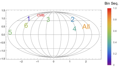
Figure 4: the maximum anisotropy directions for each one of the six considered redshift bins shown in Table 1 and in Fig. 5.

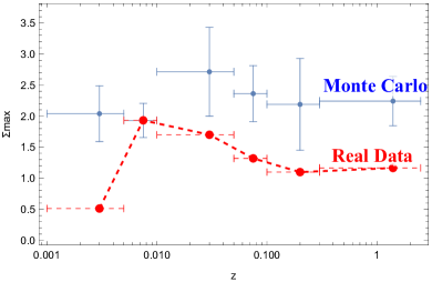
Figure 5: The value of the anisotropy level $\Sigma_{max}$ for the Pantheon+ data (red line and points) in six redshift bins. The corresponding ranges of the isotropic Monte-Carlo data are also shown (blue points).

The maximum anisotropy levels $\Sigma_{max}$ for each redshift bin along with the corresponding Monte-Carlo $1\sigma$ ranges are shown in Fig. 5. There are two points to notice in this Figure. First, there is a clear maximum in the level of anisotropy is the bin $z\in[0.005,0.01]$ (distance range $d\in[20,40]Mpc$) which is not anticipated from the Monte-Carlo ranges. This is consistent with the prediction of the off-center observer hypothesis discussed in the Introduction section I (see Fig. 1). Second, the real data appear to have systematically lower level of anisotropy in most bins than the level anticipated on the basis of Monte-Carlo simulations. This could be due to an overestimate of the uncertainties as obtained from eq. (6) and the fact that the construction of the Monte-Carlo simulations has not taken into account possible correlations among the different absolute magnitudes expressed through the covariance matrix.

In order to estimate the statistical significance of the observed shift of the anisotropy level in the first two redshift bins, in Fig. 6, we have constructed a histogram of the probability of change of $\Sigma_{max}$ in the first two redshift bins obtained from the Monte-Carlo simulations. The dashed green line corresponds to the $\Delta\Sigma_{max}$ shift for the real data. About $7\%$ of the Monte-Carlo samples had a $\Delta\Sigma_{max}$ shift equal or larger than that of the real data. This probability would get smaller if we had also demanded from the Monte-Carlo data to have a smaller $\Sigma_{max}$ on higher redshift bins as observed in the real data and as predicted in the context of the off-center observer hypothesis.

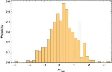
Figure 6: Probability distribution of the change of level of anisotropy between the lowest two redshift bins as obtained from the Monte-Carlo simulations. The real data value of $\Delta\Sigma_{max}$ is denoted by the dashed green line.

III.2 Isotropy of SH0ES SnIa Sample

The identified change of anisotropy level identified for the second distance bin $[20,40]Mpc$ in the Pantheon+ data is also identified in the SH0ES data of SnIa hosts hosts shown in Fig. 7. For this part of the analysis we have considered the weighted average absolute magnitude of each one of the 37 Cepheid hosts of the SH0ES data which are very weakly correlated. These absolute magnitudes and their derivation are discussed in detail in Ref. Perivolaropoulos and Skara (2023). The corresponding SH0ES data are shown in Table 2.

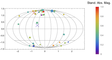
Figure 7: The angular distribution in the sky of 37 SnIa host absolute magnitudes obtained as weighted averages of the SnIa absolute magnitudes in each host. The CMB dipole direction is shown with the red cross and the maximum anisotropy axis is shown with the blue cross. Mild alignment is observed as was the case for the low distance bins of the Pantheon+ sample (see Fig. 4).

Due to the small number of hosts in the SH0ES data we have considered cumulative distance bins from low to high distances. The maximum distance $d_{max}$ of each cumulative bin was obtained from the largest distance modulus of the bin as

$$d_{max}=10^{\frac{\mu_{Ceph,max}-25}{5}}$$ (11)

where $\mu_{Ceph,max}$ maximum distance modulus of each cumulative distance bin as obtained from Cepheids. Thus each cumulative bin which includes hosts with distances in the range $d\in[d_{min},d_{max}]$ where $d_{min}=6.8Mpc$ corresponding to the closest SnIa+Cepheid host (M101) and $d_{max}$ is the maximum distance of the bin. In each distance bin we implement the hemisphere comparison method and identify the maximum anisotropy level. Thus we plot $\Sigma_{max}$ in terms of $d_{max}$ in Fig. 8. In terms of alignment of the maximum anisotropy direction with the CMB dipole we find mild alignment with the CMB dipole for the full SH0ES data. Note however that there are large uncertainties in terms of determining the anisotropy direction due to the small number of SnIa in the SH0ES data.

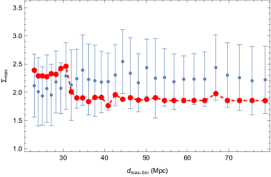
Figure 8: The anisotropy level for cumulative distance bins with maximum distance $d_{max}$ as obtained from the distance modulus of each host.

The anisotropy level for the SH0ES data shown in Fig. 8 is consistent with the corresponding results for the Pantheon+ sample. It shows a rapid decrease of the anisotropy level at $d_{max}\simeq 30Mpc$ even though the anisotropy level for all cumulative bins are consistent with the $1\sigma$ Monte-Carlo ranges shown also in Fig. 8. Due to the cumulative nature of these bins and the small number of datapoints, the lowest distance bin of the Pantheon+ analysis is not probed and thus the rapid increase of the anisotropy level is not manifest in the SH0ES data case even though the sharp decrease of the anisotropy level is clearly evident. The SH0ES data that were used for the construction of Figs 7 and 8 are shown in Table 2.

Host name	SnIa name	$\mu_{Ceph}$	$\sigma_{\mu_{Ceph}}$	$m_{B}$	$\sigma_{m_{B}}$	M	$\sigma_{M}$	RA	DEC
M101	2011fe	29.178	0.041	9.78	0.115	-19.398	0.122	210.774	54.274
N5643	2017cbv	30.546	0.052	11.229	0.054	-19.317	0.075	218.143	-44.134
N4424	2012cg	30.844	0.128	11.487	0.192	-19.357	0.230	186.803	9.420
N4536	1981B	30.835	0.05	11.551	0.133	-19.284	0.142	188.623	2.199
N1448	2021pit	31.287	0.037	12.095	0.112	-19.191	0.118	56.125	-44.632
N1365	2012fr	31.378	0.056	11.9	0.092	-19.478	0.107	53.4	-36.127
N1559	2005df	31.491	0.061	12.141	0.086	-19.35	0.105	64.407	-62.770
N2442	2015	31.45	0.064	12.234	0.082	-19.216	0.104	114.066	-69.506
N7250	2013dy	31.628	0.125	12.283	0.178	-19.345	0.217	334.573	40.570
N3982	1998aq	31.722	0.071	12.252	0.078	-19.47	0.105	179.108	55.129
N4038	2007sr	31.603	0.116	12.409	0.106	-19.194	0.157	180.47	-18.973
N3972	2011by	31.635	0.089	12.548	0.094	-19.087	0.129	178.94	55.326
N4639	1990N	31.812	0.084	12.454	0.124	-19.358	0.149	190.736	13.257
N5584	2007af	31.772	0.052	12.804	0.079	-18.968	0.094	215.588	-0.394
N3447	2012ht	31.936	0.034	12.736	0.089	-19.2	0.0953	163.345	16.776
N2525	2018gv	32.051	0.099	12.728	0.074	-19.323	0.123	121.394	-11.438
N3370	1994ae	32.12	0.051	12.937	0.082	-19.183	0.0965	161.758	17.275
N5861	2017erp	32.223	0.099	12.945	0.107	-19.278	0.146	227.312	-11.334
N5917	2005cf	32.363	0.12	13.079	0.095	-19.284	0.153	230.384	-7.413
N3254	2019np	32.331	0.076	13.201	0.074	-19.13	0.106	157.342	29.510
N3021	1995al	32.464	0.158	13.114	0.116	-19.35	0.196	147.733	33.552
N1309	2002fk	32.541	0.059	13.209	0.082	-19.332	0.101	50.523	-15.400
N4680	1997bp	32.599	0.205	13.173	0.205	-19.426	0.290	191.724	-11.642
N1015	2009ig	32.563	0.074	13.35	0.094	-19.213	0.119	39.548	-1.312
N7541	1998dh	32.5	0.119	13.418	0.128	-19.082	0.175	348.668	4.537
N2608	2001bg	32.612	0.154	13.443	0.166	-19.169	0.226	128.829	28.468
N3583	2015so	32.804	0.08	13.509	0.093	-19.295	0.123	168.654	48.318
U9391	2003du	32.848	0.067	13.525	0.084	-19.323	0.107	218.649	59.334
N0691	2005W	32.830	0.109	13.602	0.139	-19.228	0.177	27.690	21.759
N5728	2009Y	33.094	0.205	13.514	0.115	-19.580	0.235	220.599	-17.246
M1337	2006D	32.92	0.123	13.655	0.106	-19.265	0.162	193.141	-9.775
N3147	2021hpr	33.014	0.165	13.8536	0.093	-19.160	0.190	154.161	73.400
N5468	2002cr	33.116	0.074	13.942	0.053	-19.173	0.091	211.657	-5.439
N7329	2006bh	33.246	0.117	14.03	0.079	-19.216	0.141	340.067	-66.485
N7678	2002dp	33.187	0.153	14.09	0.093	-19.097	0.179	352.127	22.428
N0976	1999dq	33.709	0.149	14.25	0.103	-19.459	0.181	38.498	20.975
N0105	2007A	34.527	0.25	15.25	0.133	-19.277	0.283	6.320	12.886

Table 2: The SH0ES data that were used for the construction of Figs 7 and 8. For each host we show a representative SnIa that was used for determining the galactic coordinates of the host.

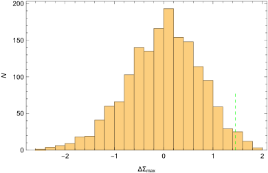
Figure 9: Histogram describing the probability of finding a change $\Delta\Sigma_{max}$ of the maximum anisotropy level, between the low distance bin for the SH0ES data. The real data value of $\Delta\Sigma_{max}=1.45$ is denoted with the green dashed line.

In order to estimate the probability that the observed sharp decrease of the anisotropy level would occur in the context of generically isotropic data we have constructed $40$ Monte-Carlo simulated SH0ES host absolute magnitude samples for each one of two distance bins: a low distance bin with $d\in[d_{min},d_{min}+20]Mpc$ and a high distance bin with $d\in[d_{min}+20]Mpc,d_{max}]$ where $d_{min}=6.8Mpc$ is the minimum SnIa+Cepheid host distance of the SH0ES sample and $d_{max}=80Mpc$ is the corresponding maximum distance. We thus have $40\times 40=1600$ bin pairs. For each pair we find the maximum anisotropy level difference $\Delta\Sigma_{max}$ and plot a histogram for the frequency of these differences in Fig. 9. For the real data we have $\Delta\Sigma_{max}=1.45$ shown with a green dashed line in Fig. 9. Only 32 of the 1600 bin pairs had a difference $\Delta\Sigma_{max}\geq 32$ ie larger than or equal to $\Delta\Sigma_{max}$ of the real data. This corresponds to a probability of about $2\%$. Thus the anisotropy level transition in the SH0ES data is fairly significant statistically (almost at $3\sigma$.

IV Discussion-Conclusion

We have used the hemisphere comparison method to investigate the level of SnIa absolute magnitude anisotropy in the Pantheon+ and SH0ES samples. Our analysis is distinct from some previous studies Sorrenti et al. (2022) in that we have not focused on the velocity dipole but on intrinsic properties of SnIa corresponding to their absolute magnitude. Also we have not considered the particular form of anisotropy described by a dipole but a general anisotropy which can be probed by the hemisphere comparison method.

We have found that for both Pantheon+ and SH0ES SnIa absolute magnitudes the anisotropy level in all bins considered is consistent with the isotropic Monte-Carlo simulated data. However, we have identified a sharp change of the level of anisotropy at the low redshift/distance bins which appears to be rare in the isotropic Monte Carlo simulated data. This change from higher level of anisotropy for absolute magnitudes of SnIa at distances $d<30Mpc$ to lower anisotropy level for absolute magnitudes of SnIa with $d>30Mpc$ is consistent with a scenario assuming an off-center observer in a $20-30Mpc$ bubble with SnIa properties that are distinct from the SnIa properties outside this bubble.

Such a scenario is also supported by previous studies which have found hints for a transition of the SnIa absolute magnitude and other astrophysical properties at $d\simeq 20Mpc$. This effect could also provide a resolution of the Hubble tension Perivolaropoulos and Skara (2022b, 2023, 2021); Marra and Perivolaropoulos (2021); Alestas et al. (2021a, b) since the value of the SnIa absolute magnitudes is closely connected and degenerate with the measured Hubble parameter $H_{0}$.

An interesting extension of the present analysis would be to use different cosmological and/or astrophysical probes like Tully-Fisher data to probe possible anisotropies of astrophysics properties in distance bins in the range of $10-50Mpc$. Such studies would provide further tests for the off-center observer interpretation of our results.

Numerical analysis files: The Mathematica v13 notebooks and data that lead to the construction of the figures of the paper may be downloaded from this url.

References

- Aluri et al. (2023) Pavan Kumar Aluri et al., “Is the observable Universe consistent with the cosmological principle?” Class. Quant. Grav. 40, 094001 (2023), arXiv:2207.05765 [astro-ph.CO] .
- Secrest et al. (2021) Nathan J. Secrest, Sebastian von Hausegger, Mohamed Rameez, Roya Mohayaee, Subir Sarkar, and Jacques Colin, “A Test of the Cosmological Principle with Quasars,” Astrophys. J. Lett. 908, L51 (2021), arXiv:2009.14826 [astro-ph.CO] .
- Zhao and Xia (2021) Dong Zhao and Jun-Qing Xia, “A tomographic test of cosmic anisotropy with the recently-released quasar sample,” Eur. Phys. J. C 81, 948 (2021).
- Hu et al. (2020) J. P. Hu, Y. Y. Wang, and F. Y. Wang, “Testing cosmic anisotropy with Pantheon sample and quasars at high redshifts,” Astron. Astrophys. 643, A93 (2020), arXiv:2008.12439 [astro-ph.CO] .
- Guandalin et al. (2022) Caroline Guandalin, Jade Piat, Chris Clarkson, and Roy Maartens, “Theoretical systematics in testing the Cosmological Principle with the kinematic quasar dipole,” (2022), arXiv:2212.04925 [astro-ph.CO] .
- Dam et al. (2022) Lawrence Dam, Geraint F. Lewis, and Brendon J. Brewer, “Testing the Cosmological Principle with CatWISE Quasars: A Bayesian Analysis of the Number-Count Dipole,” (2022), arXiv:2212.07733 [astro-ph.CO] .
- Wagenveld et al. (2023) J. D. Wagenveld et al., “The MeerKAT Absorption Line Survey: Homogeneous continuum catalogues towards a measurement of the cosmic radio dipole,” (2023), arXiv:2302.10696 [astro-ph.CO] .
- Qiang et al. (2020) Da-Chun Qiang, Hua-Kai Deng, and Hao Wei, “Cosmic Anisotropy and Fast Radio Bursts,” Class. Quant. Grav. 37, 185022 (2020), arXiv:1902.03580 [astro-ph.CO] .
- Singal (2023) Ashok K. Singal, “Discordance of dipole asymmetries seen in recent large radio surveys with the Cosmological Principle,” (2023), arXiv:2303.05141 [astro-ph.CO] .
- Watkins et al. (2023) Richard Watkins, Trey Allen, Collin James Bradford, Albert Ramon, Alexandra Walker, Hume A. Feldman, Rachel Cionitti, Yara Al-Shorman, Ehsan Kourkchi, and R. Brent Tully, “Analyzing the Large-Scale Bulk Flow using CosmicFlows4: Increasing Tension with the Standard Cosmological Model,” (2023), arXiv:2302.02028 [astro-ph.CO] .
- Watkins and Feldman (2015) Richard Watkins and Hume A. Feldman, “Large-scale bulk flows from the Cosmicflows-2 catalogue,” Mon. Not. Roy. Astron. Soc. 447, 132–139 (2015), arXiv:1407.6940 [astro-ph.CO] .
- Wiltshire et al. (2013) David L. Wiltshire, Peter R. Smale, Teppo Mattsson, and Richard Watkins, “Hubble flow variance and the cosmic rest frame,” Phys. Rev. D 88, 083529 (2013), arXiv:1201.5371 [astro-ph.CO] .
- Nadolny et al. (2021) Tobias Nadolny, Ruth Durrer, Martin Kunz, and Hamsa Padmanabhan, “A new way to test the Cosmological Principle: measuring our peculiar velocity and the large-scale anisotropy independently,” JCAP 11, 009 (2021), arXiv:2106.05284 [astro-ph.CO] .
- Atrio-Barandela et al. (2015) Fernando Atrio-Barandela, Alexander Kashlinsky, Harald Ebeling, Dale J. Fixsen, and Dale Kocevski, “Probing the Dark Flow Signal in Wmap 9 -year and Planck Cosmic Microwave Background Maps,” Astrophys. J. 810, 143 (2015), arXiv:1411.4180 [astro-ph.CO] .
- Copi et al. (2010) Craig J. Copi, Dragan Huterer, Dominik J. Schwarz, and Glenn D. Starkman, “Large angle anomalies in the CMB,” Adv. Astron. 2010, 847541 (2010), arXiv:1004.5602 [astro-ph.CO] .
- Schwarz et al. (2016) Dominik J. Schwarz, Craig J. Copi, Dragan Huterer, and Glenn D. Starkman, “CMB Anomalies after Planck,” Class. Quant. Grav. 33, 184001 (2016), arXiv:1510.07929 [astro-ph.CO] .
- Tempel and Libeskind (2013) Elmo Tempel and Noam I. Libeskind, “Galaxy spin alignment in filaments and sheets: observational evidence,” Astrophys. J. Lett. 775, L42 (2013), arXiv:1308.2816 [astro-ph.CO] .
- Simonte et al. (2023) Marco Simonte, Heinz Andernach, Marcus Brueggen, Philip Best, and Erik Osinga, “Revisiting the alignment of radio galaxies in the ELAIS-N1 field,” Astron. Astrophys. 672, A178 (2023), arXiv:2303.00773 [astro-ph.GA] .
- Shamir (2022) Lior Shamir, “New evidence and analysis of cosmological-scale asymmetry in galaxy spin directions,” J. Astrophys. Astron. 43, 24 (2022), arXiv:2201.03757 [astro-ph.CO] .
- Bengaly et al. (2017) C. A. P. Bengaly, A. Bernui, J. S. Alcaniz, H. S. Xavier, and C. P. Novaes, “Is there evidence for anomalous dipole anisotropy in the large-scale structure?” Mon. Not. Roy. Astron. Soc. 464, 768–774 (2017), arXiv:1606.06751 [astro-ph.CO] .
- Sorrenti et al. (2022) Francesco Sorrenti, Ruth Durrer, and Martin Kunz, “The Dipole of the Pantheon+SH0ES Data,” (2022), arXiv:2212.10328 [astro-ph.CO] .
- McConville and Colgáin (2023) Ruairí McConville and Eoin Ó. Colgáin, “Anisotropic Distance Ladder in Pantheon+ Supernovae,” (2023), arXiv:2304.02718 [astro-ph.CO] .
- Perivolaropoulos and Skara (2022a) Leandros Perivolaropoulos and Foteini Skara, “Challenges for CDM: An update,” New Astron. Rev. 95, 101659 (2022a), arXiv:2105.05208 [astro-ph.CO] .
- Peebles (2022) Phillip James E. Peebles, “Anomalies in physical cosmology,” Annals Phys. 447, 169159 (2022), arXiv:2208.05018 [astro-ph.CO] .
- Abdalla et al. (2022) Elcio Abdalla et al., “Cosmology intertwined: A review of the particle physics, astrophysics, and cosmology associated with the cosmological tensions and anomalies,” JHEAp 34, 49–211 (2022), arXiv:2203.06142 [astro-ph.CO] .
- Heymans et al. (2021) Catherine Heymans et al., “KiDS-1000 Cosmology: Multi-probe weak gravitational lensing and spectroscopic galaxy clustering constraints,” Astron. Astrophys. 646, A140 (2021), arXiv:2007.15632 [astro-ph.CO] .
- Troxel et al. (2018) M.A. Troxel et al. (DES), “Survey geometry and the internal consistency of recent cosmic shear measurements,” Mon. Not. Roy. Astron. Soc. 479, 4998–5004 (2018), arXiv:1804.10663 [astro-ph.CO] .
- Asgari et al. (2020) Marika Asgari et al., “KiDS+VIKING-450 and DES-Y1 combined: Mitigating baryon feedback uncertainty with COSEBIs,” Astron. Astrophys. 634, A127 (2020), arXiv:1910.05336 [astro-ph.CO] .
- van Uitert et al. (2018) Edo van Uitert et al., “KiDS+GAMA: cosmology constraints from a joint analysis of cosmic shear, galaxy–galaxy lensing, and angular clustering,” Mon. Not. Roy. Astron. Soc. 476, 4662–4689 (2018), arXiv:1706.05004 [astro-ph.CO] .
- Solà Peracaula et al. (2018) Joan Solà Peracaula, Javier de Cruz Pérez, and Adrià Gómez-Valent, “Dynamical dark energy vs. = const in light of observations,” EPL 121, 39001 (2018), arXiv:1606.00450 [gr-qc] .
- Anand et al. (2017) Sampurn Anand, Prakrut Chaubal, Arindam Mazumdar, and Subhendra Mohanty, “Cosmic viscosity as a remedy for tension between PLANCK and LSS data,” JCAP 11, 005 (2017), arXiv:1708.07030 [astro-ph.CO] .
- Di Valentino et al. (2021) Eleonora Di Valentino, Olga Mena, Supriya Pan, Luca Visinelli, Weiqiang Yang, Alessandro Melchiorri, David F. Mota, Adam G. Riess, and Joseph Silk, “In the realm of the Hubble tension—a review of solutions,” Class. Quant. Grav. 38, 153001 (2021), arXiv:2103.01183 [astro-ph.CO] .
- Di Valentino et al. (2017) Eleonora Di Valentino, Alessandro Melchiorri, Eric V. Linder, and Joseph Silk, “Constraining Dark Energy Dynamics in Extended Parameter Space,” Phys. Rev. D 96, 023523 (2017), arXiv:1704.00762 [astro-ph.CO] .
- Wang (2020) Deng Wang, “Can gravity relieve and tensions?” (2020), arXiv:2008.03966 [astro-ph.CO] .
- Gómez-Valent and Solà (2017) Adria Gómez-Valent and Joan Solà, “Relaxing the -tension through running vacuum in the Universe,” EPL 120, 39001 (2017), arXiv:1711.00692 [astro-ph.CO] .
- Di Valentino and Bridle (2018) Eleonora Di Valentino and Sarah Bridle, “Exploring the Tension between Current Cosmic Microwave Background and Cosmic Shear Data,” Symmetry 10, 585 (2018).
- Tsagas (2022) Christos G. Tsagas, “The deceleration parameter in ‘tilted’ universes: generalising the Friedmann background,” Eur. Phys. J. C 82, 521 (2022), arXiv:2112.04313 [gr-qc] .
- Asvesta et al. (2022) Kerkyra Asvesta, Lavrentios Kazantzidis, Leandros Perivolaropoulos, and Christos G. Tsagas, “Observational constraints on the deceleration parameter in a tilted universe,” Mon. Not. Roy. Astron. Soc. 513, 2394–2406 (2022), arXiv:2202.00962 [astro-ph.CO] .
- Tsagas (2021) Christos G. Tsagas, “The peculiar Jeans length,” Eur. Phys. J. C 81, 753 (2021), arXiv:2103.15884 [gr-qc] .
- Tsagas (2010) Christos G Tsagas, “Large-scale peculiar motions and cosmic acceleration,” Mon. Not. Roy. Astron. Soc. 405, 503 (2010), arXiv:0902.3232 [astro-ph.CO] .
- Colgáin (2019) Eoin Ó. Colgáin, “A hint of matter underdensity at low z?” JCAP 09, 006 (2019), arXiv:1903.11743 [astro-ph.CO] .
- Krishnan et al. (2021) Chethan Krishnan, Roya Mohayaee, Eoin Ó. Colgáin, M. M. Sheikh-Jabbari, and Lu Yin, “Does Hubble tension signal a breakdown in FLRW cosmology?” Class. Quant. Grav. 38, 184001 (2021), arXiv:2105.09790 [astro-ph.CO] .
- Brout et al. (2022a) Dillon Brout et al., “The Pantheon+ Analysis: Cosmological Constraints,” Astrophys. J. 938, 110 (2022a), arXiv:2202.04077 [astro-ph.CO] .
- Scolnic et al. (2022) Dan Scolnic et al., “The Pantheon+ Analysis: The Full Data Set and Light-curve Release,” Astrophys. J. 938, 113 (2022), arXiv:2112.03863 [astro-ph.CO] .
- Brout et al. (2022b) Dillon Brout et al., “The Pantheon+ Analysis: SuperCal-fragilistic Cross Calibration, Retrained SALT2 Light-curve Model, and Calibration Systematic Uncertainty,” Astrophys. J. 938, 111 (2022b), arXiv:2112.03864 [astro-ph.CO] .
- Scolnic et al. (2018) D. M. Scolnic et al. (Pan-STARRS1), “The Complete Light-curve Sample of Spectroscopically Confirmed SNe Ia from Pan-STARRS1 and Cosmological Constraints from the Combined Pantheon Sample,” Astrophys. J. 859, 101 (2018), arXiv:1710.00845 [astro-ph.CO] .
- Horstmann et al. (2022) Nick Horstmann, Yannic Pietschke, and Dominik J. Schwarz, “Inference of the cosmic rest-frame from supernovae Ia,” Astron. Astrophys. 668, A34 (2022), arXiv:2111.03055 [astro-ph.CO] .
- Zhai and Percival (2022) Zhongxu Zhai and Will J. Percival, “Sample variance for supernovae distance measurements and the Hubble tension,” Phys. Rev. D 106, 103527 (2022), arXiv:2207.02373 [astro-ph.CO] .
- Krishnan et al. (2022a) Chethan Krishnan, Roya Mohayaee, Eoin Ó. Colgáin, M. M. Sheikh-Jabbari, and L. Yin, “Hints of FLRW breakdown from supernovae,” Phys. Rev. D 105, 063514 (2022a), arXiv:2106.02532 [astro-ph.CO] .
- Krishnan et al. (2022b) Chethan Krishnan, Ranjini Mondol, and M. M. Sheikh-Jabbari, “A Tilt Instability in the Cosmological Principle,” (2022b), arXiv:2211.08093 [astro-ph.CO] .
- Luongo et al. (2022) Orlando Luongo, Marco Muccino, Eoin Ó. Colgáin, M. M. Sheikh-Jabbari, and Lu Yin, “Larger H0 values in the CMB dipole direction,” Phys. Rev. D 105, 103510 (2022), arXiv:2108.13228 [astro-ph.CO] .
- Zhai and Percival (2023) Zhongxu Zhai and Will J. Percival, “The effective volume of supernovae samples and sample variance,” (2023), arXiv:2303.05717 [astro-ph.CO] .
- Marra and Perivolaropoulos (2021) Valerio Marra and Leandros Perivolaropoulos, “A rapid transition of at as a possible solution of the Hubble and growth tensions,” Phys. Rev. D 104, L021303 (2021), arXiv:2102.06012 [astro-ph.CO] .
- Alestas et al. (2021a) George Alestas, Lavrentios Kazantzidis, and Leandros Perivolaropoulos, “ phantom transition at 0.1 as a resolution of the Hubble tension,” Phys. Rev. D 103, 083517 (2021a), arXiv:2012.13932 [astro-ph.CO] .
- Perivolaropoulos and Skara (2022b) Leandros Perivolaropoulos and Foteini Skara, “A Reanalysis of the Latest SH0ES Data for H0: Effects of New Degrees of Freedom on the Hubble Tension,” Universe 8, 502 (2022b), arXiv:2208.11169 [astro-ph.CO] .
- Riess et al. (2022) Adam G. Riess et al., “A Comprehensive Measurement of the Local Value of the Hubble Constant with 1 km s-1 Mpc-1 Uncertainty from the Hubble Space Telescope and the SH0ES Team,” Astrophys. J. Lett. 934, L7 (2022), arXiv:2112.04510 [astro-ph.CO] .
- Perivolaropoulos and Skara (2023) Leandros Perivolaropoulos and Foteini Skara, “On the homogeneity of SnIa absolute magnitude in the Pantheon+ sample,” Mon. Not. Roy. Astron. Soc. 520, 5110–5125 (2023), arXiv:2301.01024 [astro-ph.CO] .
- Alestas et al. (2021b) George Alestas, Ioannis Antoniou, and Leandros Perivolaropoulos, “Hints for a Gravitational Transition in Tully–Fisher Data,” Universe 7, 366 (2021b), arXiv:2104.14481 [astro-ph.CO] .
- Perivolaropoulos (2022) Leandros Perivolaropoulos, “Is the Hubble Crisis Connected with the Extinction of Dinosaurs?” Universe 8, 263 (2022), arXiv:2201.08997 [astro-ph.EP] .
- Schwarz and Weinhorst (2007) Dominik J. Schwarz and Bastian Weinhorst, “(An)isotropy of the Hubble diagram: Comparing hemispheres,” Astron. Astrophys. 474, 717–729 (2007), arXiv:0706.0165 [astro-ph] .
- Antoniou and Perivolaropoulos (2010) I. Antoniou and L. Perivolaropoulos, “Searching for a Cosmological Preferred Axis: Union2 Data Analysis and Comparison with Other Probes,” JCAP 12, 012 (2010), arXiv:1007.4347 [astro-ph.CO] .
- Mariano and Perivolaropoulos (2013) Antonio Mariano and Leandros Perivolaropoulos, “CMB Maximum temperature asymmetry Axis: Alignment with other cosmic asymmetries,” Phys. Rev. D 87, 043511 (2013), arXiv:1211.5915 [astro-ph.CO] .
- Mariano and Perivolaropoulos (2012) Antonio Mariano and Leandros Perivolaropoulos, “Is there correlation between Fine Structure and Dark Energy Cosmic Dipoles?” Phys. Rev. D 86, 083517 (2012), arXiv:1206.4055 [astro-ph.CO] .
- Deng and Wei (2018a) Hua-Kai Deng and Hao Wei, “Testing the Cosmic Anisotropy with Supernovae Data: Hemisphere Comparison and Dipole Fitting,” Phys. Rev. D 97, 123515 (2018a), arXiv:1804.03087 [astro-ph.CO] .
- Chang and Lin (2015) Zhe Chang and Hai-Nan Lin, “Comparison between hemisphere comparison method and dipole-fitting method in tracing the anisotropic expansion of the Universe use the Union2 dataset,” Mon. Not. Roy. Astron. Soc. 446, 2952–2958 (2015), arXiv:1411.1466 [astro-ph.CO] .
- Kazantzidis and Perivolaropoulos (2020) L. Kazantzidis and L. Perivolaropoulos, “Hints of a Local Matter Underdensity or Modified Gravity in the Low Pantheon data,” Phys. Rev. D 102, 023520 (2020), arXiv:2004.02155 [astro-ph.CO] .
- Deng and Wei (2018b) Hua-Kai Deng and Hao Wei, “Null signal for the cosmic anisotropy in the Pantheon supernovae data,” Eur. Phys. J. C 78, 755 (2018b), arXiv:1806.02773 [astro-ph.CO] .
- Duffett-Smith and Zwart (2011) Peter Duffett-Smith and Jonathan Zwart, Practical Astronomy with your Calculator or Spreadsheet, 4th ed. (Cambridge University Press, 2011).
- Perivolaropoulos and Skara (2021) Leandros Perivolaropoulos and Foteini Skara, “Hubble tension or a transition of the Cepheid SnIa calibrator parameters?” Phys. Rev. D 104, 123511 (2021), arXiv:2109.04406 [astro-ph.CO] .