Relabeling Minimal Training Subset to Flip a Prediction

Abstract

When facing an unsatisfactory prediction from a machine learning model, users can be interested in investigating the underlying reasons and exploring the potential for reversing the outcome. We ask: To flip the prediction on a test point $x_{t}$, how to identify the smallest training subset $\mathcal{S}_{t}$ that we need to relabel? We propose an efficient algorithm to identify and relabel such a subset via an extended influence function for binary classification models with convex loss. We find that relabeling fewer than 2% of the training points can always flip a prediction. This mechanism can serve multiple purposes: (1) providing an approach to challenge a model prediction by altering training points; (2) evaluating model robustness with the cardinality of the subset (i.e., $|\mathcal{S}_{t}|$); we show that $|\mathcal{S}_{t}|$ is highly related to the noise ratio in the training set and $|\mathcal{S}_{t}|$ is correlated with but complementary to predicted probabilities; and (3) revealing training points lead to group attribution bias. To the best of our knowledge, we are the first to investigate identifying and relabeling the minimal training subset required to flip a given prediction.

1 Introduction

The interpretability of machine learning systems is a crucial research area as it aids in understanding model behavior, facilitating debugging, and enhancing performance (Adebayo et al., 2020; Han et al., 2020; Pezeshkpour et al., 2022; Teso et al., 2021; Marx et al., 2019). A common approach involves analyzing the model’s predictions by tracing back to the training data (Hampel, 1974; Cook and Weisberg, 1980, 1982). Particularly, when a machine learning model produces an undesirable result, users might be interested in identifying the training points to modify to overturn the outcome. If the identified training points are wrongly labeled, the related determination should be overturned. For instance, consider a scenario where a machine learning model evaluates research papers and gives decisions. If an author receives a rejection and disagrees with the result, they might request insight into the specific papers examples used to train the model. If it turns out that correcting a few mislabeled training examples can change the prediction, then the original decision might need reconsideration, possibly accepting the paper instead. This concept is referred to contesting the predictions made by automatic models (Hirsch et al., 2017; Vaccaro et al., 2019). When using such models, users should have the right and ability to question and challenge results, especially when these results impact them directly (Almada, 2019). Our research is geared towards offering a mechanism for users to challenge these predictions by tracing back to the training data.

Figure 1: The question we seek to answer is: which is the smallest subset of the training data that needs to be relabeled in order to flip a specific prediction from the model?

Test Point			$|\mathcal{S}_{t}|$	Indentified Training Subset $\mathcal{S}_{t}$
Text	Label	Prediction		Text	Mislabeled as
The people who can stop it are the ones who pay their wages.	Non-hate	Hate	1	Worker.	Hate
We will never forget their heroism.	Non-hate	Hate	1	TRUTH NO LIE.	Hate

Table 1: Examples showcase misclassified test points alongside the identified training set $\mathcal{S}_{t}$. For each test point, if those training points are relabeled prior to training, the test point can be correctly classified. These training points are intentional noise we manually introduced into the dataset.

In this paper, we study the question (visualized in Figure 1): Given a test point $x_{t}$ and its associated predicted label $\hat{y}_{t}$ by a model, how can we find the minimal training subset $\mathcal{S}_{t}$, if relabeled before training, would lead to a different prediction?

Identifying $\mathcal{S}_{t}$ by enumerating all possible subsets of training examples, re-training under each, and then observing the resultant prediction would be inefficient and impractical. We thus introduce an algorithm for finding such sets efficiently using the extended influence function, which allow us to approximate changes in predictions expected as a result of relabeling subsets of training data Koh et al. (2019); Warnecke et al. (2021a); Kong et al. (2021).

The identified subset $\mathcal{S}_{t}$ can be harnessed for a variety of downstream applications. Firstly, we discover that $|\mathcal{S}_{t}|$ can be less than 2% of the total number of training points, suggesting that relabeling a small fraction of the training data can markedly influence the test prediction. Secondly, we observe a correlation between $|\mathcal{S}_{t}|$ and the noise ratio in the training set. As the noise ratio increases from 0 to 0.5, $|\mathcal{S}_{t}|$ tends to decrease obviously. Thirdly, we find that $|\mathcal{S}_{t}|$ can be small when the model is highly confident in a test prediction, so $|\mathcal{S}_{t}|$ serves as a measure of robustness that complements to the predicted probability. Lastly, our approach can shed light on points containing group attribution bias that caused biased determinations. We demonstrate that when such bias exists in the training set, the corresponding $\mathcal{S}_{t}$ will significantly overlap with the biased training set.

The contributions of this work are summarized as follows. (1) We introduce the problem: identifying the minimal subset $\mathcal{S}_{t}$ of training data, if relabeled, would result in a different prediction on test point $x_{t}$; (2) We provide a computationally efficient algorithm for binary classification models with convex loss and report performance in text classification problems; (3) We demonstrate that the size of the subset ($|\mathcal{S}_{t}|$) can be used to assess the robustness of the model and the training set; (4) We show that the composition of $\mathcal{S}_{t}$ can explain group attribution bias.

2 Methods

This section first demonstrates the algorithm to find the minimal relabel set and shows a case to use the algorithm to challenge the model’s prediction.

2.1 Algorithm

Consider a binary classification problem with a training dataset denoted as $\mathcal{Z}^{\text{tr}}=\{z_{1},\ldots,z_{N}\}$. Each data point $z_{i}=(x_{i},y_{i})$ consists of features $x_{i}\in\mathcal{X}$ and a label $y_{i}\in\mathcal{Y}$. We train a classification model $f_{w}:\mathcal{X}\rightarrow\mathcal{Y}$, where $f$ is parameterized by a parameter vector $w\in\mathbb{R}^{p}$. By minimizing the empirical risk, this process yields the estimated parameter $\hat{w}$, defined by:

$$~{}\begin{aligned} \hat{w}&:=\underset{w}{\text{argmin}}\,\mathcal{R}(w)\\ &=\underset{w}{\text{argmin}}\left(\frac{1}{N}\sum_{i=1}^{N}\mathcal{L}(z_{i},w)+\frac{\lambda}{2}\|w\|^{2}\right)\end{aligned}$$ (1)

$\mathcal{L}(z_{i},w)$ represents the loss function that measures the prediction error for a single data point $z_{i}$ given the parameters $w$, and $\mathcal{R}(w)$ denotes the total empirical risk, which includes a regularization term controlled by the hyperparameter $\lambda$. We assume that $\mathcal{R}$ is twice-differentiable and strongly convex in $w$, with the Hessian matrix $H_{\hat{w}}:=\nabla_{w}^{2}\mathcal{R}(\hat{w})=\frac{1}{N}\sum_{i=1}^{N}\nabla_{w}^{2}\mathcal{L}(z_{i},\hat{w})+{\lambda}\mathit{I}$.

Suppose we relabel a subset of the training points $\mathcal{S}\subset\mathcal{Z}^{\text{tr}}$ by changing $y_{i}$ to $y_{i}^{\prime}$ for each $(x_{i},y_{i})\in\mathcal{S}$ and then re-estimate $w$ to minimize $\mathcal{R}(w)$, resulting in new parameters $\hat{w}_{\mathcal{S}}$:

$$\hat{w}_{\mathcal{S}}=\underset{w}{\text{argmin}}\left(\mathcal{R}(w)+\frac{1}{N}\sum_{(x_{i},y_{i})\in\mathcal{S}}\ell\right)$$ (2)

where $\ell=-\mathcal{L}(x_{i},y_{i},w)+\mathcal{L}(x_{i},y_{i}^{\prime},w)$ represents the adjustment to the original loss due to the relabeling of points in $\mathcal{S}$.

Due to the large number of possible subsets in the training set, it is computationally impractical to relabel and retrain models for each subset to observe prediction changes. Warnecke et al. (2021b); Kong et al. (2021) derived the influence exerted by relabeling a training set $\mathcal{S}$ on the loss incurred for a test point $t$ as:

$$\nabla_{w}\mathcal{L}(z_{t},\hat{w})^{\intercal}{\Delta_{i}w},$$ (3)

where $\Delta_{i}w=\frac{1}{N}H^{-1}_{\hat{w}}\sum_{(x_{i},y_{i})\in S}\nabla_{w}\ell$ is the change of parameters after relabeling training points in $\mathcal{S}$. Instead, we estimate the influence on predicted probability result by relabeling the training subset $\mathcal{S}$ as:

$$\Delta_{t}f:=\nabla_{w}f_{\hat{w}}(x_{t})^{\intercal}\Delta_{i}w,$$ (4)

which is named as IP-relabel.

Based on this IP-relabel and adopting the algorithm proposed by Broderick et al. (2020); Yang et al. (2023), we propose the Algorithm 1 to find a training subset $\mathcal{S}_{t}$ to relabel, which would result in flipping the test prediction $\hat{y}_{t}$ on $x_{t}$. Our approach initiates by approximating the change in predicted probability $\Delta_{t}f$ for a test point $x_{t}$, which results from the relabeling of each training point. Subsequently, we iterate through all the training points in a descending order of their influence from the most decisive to the least. During each iteration, we accumulate the change in predicted probability $\Delta_{t}f$. When the cumulative change causes the output $\hat{y}_{t}$ to cross a predefined threshold, the algorithm identifies $\mathcal{S}_{t}$. If, however, the output fails to cross the threshold even after examining the entire training set, the algorithm is unable to find the set $\mathcal{S}_{t}$. For $N$ training points and the parameter $w$ in $\mathbb{R}^{p}$, our algorithm requires $O(p^{3})$ to compute the inverse of the Hessian matrix for the total loss and $O(Np^{2})$ to calculate the IP-relabel for each training point. Therefore, the overall computational complexity is $O(p^{3}+Np^{2})$. We also include the running time of our experiments in Appendix A.3.

2.2 Case Study

In this section, we present an example to demonstrate how our method can be used to challenge the predictions of machine learning models. We employ the Hate Speech dataset (de Gibert et al., 2018), which encompasses instances of hate communication that target specific groups based on characteristics such as race, color, ethnicity, etc. On social media platforms, users found engaging in hate speech are typically banned.

We implement a linear regression model to classify hate speech on the internet. We intentionally introduced noise into the training dataset by mislabeling 1,000 data points (out of 9632, switching labels from 1 to 0 and vice versa). This deliberate noise in the training set can result in additional misclassifications during model testing.

As demonstrated in Table 1, for each test instance, Algorithm 1 pinpoints the specific training data points that, when relabeled before training, could change the prediction of the test point. The table showcases two instances where the model misclassified test points. The corresponding training sets, $\mathcal{S}_{t}$, consist of training points that closely resemble the test cases but were erroneously labeled. Given that the classifications can be altered by relabeling the small subset of mislabeled training data, determinations based on these classifications, such as banning users, warrant careful reconsideration.

Input: $f$: Model; $\mathcal{Z}^{\text{tr}}$: Full training set; $N$: number of total training points; $\mathcal{Z}^{\text{tr}\textquoteright}$: Relabeled full training set; $\hat{w}$: Parameters estimated $\mathcal{Z}^{\text{tr}}$; $\mathcal{L}$: Loss function; $x_{t}$: A test point; $\tau$: Classification threshold (e.g., 0.5)

Output: $\mathcal{S}_{t}$: minimal train subset identified to flip the prediction ($\emptyset$ if unsuccessful)

1 $H\leftarrow\nabla_{w}^{2}\mathcal{L}(\mathcal{Z}^{\text{tr}},\hat{w})$

2 $\nabla_{w}l\leftarrow-\nabla_{w}\mathcal{L}(\mathcal{Z}^{\text{tr}},\hat{w})+\nabla_{w}\mathcal{L}(\mathcal{Z}^{\text{tr}^{\prime}},\hat{w})$

3 $\Delta w\leftarrow\frac{1}{N}H^{-1}\nabla_{w}l$

4 $\Delta_{t}f\leftarrow\nabla_{w}f_{\hat{w}}(x_{t})^{\intercal}\Delta w$

$\hat{y}_{t}\leftarrow f(x_{t})>\tau$

  // Binary prediction

// Sort instances (and estimated output differences) in order of the current prediction

5 ${\tt direction}\leftarrow\{\uparrow$ if $\hat{y}_{t}$ else $\downarrow$}

6 ${\tt indices}\leftarrow{\tt argsort}(\Delta_{t}f,{\tt direction})$

7 $\Delta_{t}f\leftarrow{\text{\tt sort}}(\Delta_{t}f,{\tt direction})$

8

9for $k=1$ … $|\mathcal{Z}^{\text{tr}}|$ do

10       $\hat{y}_{t}^{\prime}=(f(x_{t})+{\text{\tt sum}}(\Delta_{t}f[:k]))>\tau$ if $\hat{y}^{\prime}_{t}\neq\hat{y}_{t}$ then

11             return $\mathcal{Z}^{\text{tr}}[{\tt indices}[:k]]$

12      

return $\emptyset$

Algorithm 1 An algorithm to find a minimal subset to flip a test prediction

3 Experiments

We provide an overview of our experiments:

1. We introduce our experimental setup and then validate Algorithm 1 in Sec 3.1 and 3.2. Our results confirm that we can effectively change the test predictions by relabeling revealed points and subsequent model retraining.

2. Sec 3.3 analyzes the magnitude of $|\mathcal{S}_{t}|$ across various datasets and models, emphasizing its correlation with predicted probability and noise ratio. This showcases its utility in analyzing the robustness of training points and models.

3. We further delve into the integration of subset $\mathcal{S}_{t}$ in Sec 3.4, demonstrating its potential to highlight biased training data.

4. In Sec 3.5, we compare our method against other methods to alter training points to flip test prediction, illustrating that our method revealed a smaller training subset.

3.1 Experimental Setting

Datasets. We use a tabular dataset: Loan default classification Surana (2021), and text datasets: Movie review sentiment Socher et al. (2013); Essay grading Foundation (2010); Hate speech de Gibert et al. (2018); and Twitter sentiment Go et al. (2009) to evaluate our method.

Models. We consider the $l_{2}$ regularized logistic regression to fit the assumption on influence function. As features, we consider both bag-of-words and neural embeddings induced via BERT Devlin et al. (2018) for text datasets. We report basic statistics describing our datasets and model performance in Section A.1.

Dataset	Features	Found $\mathcal{S}_{t}$	Flip Successful	Successful Ratio
Loan	BoW	61%	49%	80%
Movie	BoW	100%	72%	72%
reviews	BERT	100%	73%	73%
Essays	BoW	77%	40%	52%
	BERT	76%	39%	51%
Hate	BoW	99%	87%	87%
speech	BERT	99%	86%	87%
Tweet	BoW	100%	75%	75%
sentiment	BERT	100%	68%	68%

Table 2: Percentages of text examples for which Algorithm 1 successfully identified a set $\mathcal{S}_{t}$ (2nd column) and for which upon flipping these instances and retraining the prediction indeed flipped (3rd column). The "Successful Ratio" is obtained by divide the percentages in the "Flip Successful" column by those in the "Found $\mathcal{S}_{t}$" column.

3.2 Algorithm Validation

How effective is our algorithm at finding $\mathcal{S}_{t}$ and flipping the corresponding prediction? As shown in Table 2, the frequency of finding $\mathcal{S}_{t}$ varies greatly among datasets. For the movie reviews and tweet datasets, Algorithm 1 returns a set $\mathcal{S}_{t}$ for approximately 100% of test points. On the other hand, for the simpler loan data, it only returns $\mathcal{S}_{t}$ for approximately 60% of instances. Results for other datasets fall between these two extremes. When the algorithm successfully finds a set $\mathcal{S}_{t}$, relabeling all $(x_{i},y_{i})\in\mathcal{S}_{t}$ almost enables the re-trained model to flip the prediction $\hat{y}_{t}$ (as indicated in the right-most column of Table 2).

Comparison with other methods. We draw comparisons between IP-relabel and several other methods (Pezeshkpour et al., 2021), including IP-remove (Yang et al., 2023), influence function (Koh and Liang, 2017), and three gradient-based instance attribution methods on a logistic regression model to the movie review dataset (Barshan et al., 2020; Charpiat et al., 2019):

1. $RIF=cos(H^{-\frac{1}{2}}\nabla_{w}\mathcal{L}(x_{t}),H^{-\frac{1}{2}}\nabla_{w}\mathcal{L}(x_{i}))$

2. $GD=\left<\nabla_{w}\mathcal{L}(x_{t}),\nabla_{w}\mathcal{L}(x_{i})\right>$

3. $GC=cos(\nabla_{w}\mathcal{L}(x_{t}),\nabla_{w}\mathcal{L}(x_{i}))$

We also randomly select subsets of training data and relabel them. We graph the average change in predicted probability for 100 randomly chosen test points in Figure 2. These probabilities are from the model trained before and after relabeling the top $k$ training points ranked on the scores above. Our analysis indicates that IP-relabel shows a more significant impact in the test predicted probability compared to the impact of removing training points as ranked by other methods.

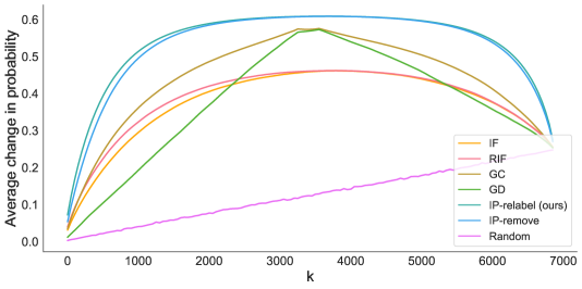
Figure 2: The relationship between the average of absolute difference on predicted probabilities for sampled test points results from relabeled $k=|\mathcal{S}_{t}|$ training points, using different methods on movie review dataset.

Running time of Algorithm 1. We recorded the average running time of Algorithm 1 to find $\mathcal{S}_{t}$ for test points in different datasets in Table 8 on Apple M1 Pro CPUs. For one test point, it just takes milliseconds to go through the whole training set (the training set sizes are provided in A.1) to find $\mathcal{S}_{t}$.

Dataset	BoW (ms)	BERT (ms)
Movie Reviews	19.04	140.51
Essays	160.01	265.09
Hate speech	103.70	299.46
Tweet	58.42	260.75
Loan	63.97	/

Table 3: Average running time (in milliseconds) of Algorithm 1 to find $\mathcal{S}_{t}$ for a test point in different datasets.

3.3 $|\mathcal{S}_{t}|$ Quantifies Model Robustness

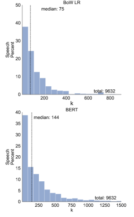
Figure 3: The histogram shows the distribution of $k=|\mathcal{S}_{t}|$ on the hate speech dataset, i.e. the minimal number of points that need to be relabeled from the training data to change the prediction $\hat{y}_{t}$ of a specific test example $x_{t}$.

Relabeling less than 2% training data can usually flip a prediction. The empirical distributions of $k$ values for subsets $\mathcal{S}_{t}$ identified by Algorithm 1 can be seen in Figure 3 for the representative hate speech datasets (full results are in the Appendix). The key observation is that when $\mathcal{S}_{t}$ is found, its size is often relatively small compared to the total number of training instances. In fact, for many test points, relabeling less than 2% instances would have resulted in a flipped prediction.

BERT demonstrates greater robustness than LR based on $|\mathcal{S}_{t}|$ measures. For a proficiently trained model, relabeling a larger subset of training data in order to alter a correct test prediction suggests greater model robustness. In Figure 4, we present a comparison of the average values of $|\mathcal{S}_{t}|$ for common test data points where both BERT and LR model predictions were successfully altered using our method. The results indicate that BERT typically demands the relabeling of more training data points than the LR models do. This observation supports the utility of our method in gauging the relative robustness of different models.

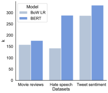
Figure 4: Comparison of the average $k=|\mathcal{S}_{t}|$ values for shared test points under both BERT and LR models that were successfully flipped by our method.

Correlation between $k$ and the predicted probability. Does the size of $\mathcal{S}_{t}$ tell us anything beyond what we might infer from the predicted probability $p(y_{t}=1)$? In Fig 5 we show a scatter of $k=|\mathcal{S}_{t}|$ against the distance of the predicted probability from 0.5 on speech dataset. There are test instances of the model being confident, but relabeling a small set of training instances would overturn the prediction. In Sec A.4, there are datasets where the $k$ can be highly correlated with probability.

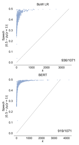
Figure 5: The correlation between the predicted probabilities of certain test examples and $k=|\mathcal{S}_{t}|$ on the hate speech dataset. For test examples where the model is highly certain about its prediction, the prediction can be flipped by relabeling a small number of data points from the training set.

How is $|\mathcal{S}_{t}|$ correlated with the noise ratio? Figure 6 shows how $|\mathcal{S}_{t}|$ and the model’s accuracy vary when we increase the noise ratio from 0 to 0.9. We introduce noise to the training set by incrementally relabeling a portion of training points, from 0 to 0.9 in steps of 0.1. When the noise ratio increases from 0 to 0.5, we observe a decline in $|\mathcal{S}_{t}|$. However, as the noise ratio rises from 0.5 to 0.9, $|\mathcal{S}_{t}|$ starts to increase. Interestingly, within the noise ratio interval of 0 to 0.3, the model’s accuracy does not demonstrate a noticeable decline. This suggests that $|\mathcal{S}_{t}|$ can be an additional metric for assessing the model’s robustness complementary to accuracy under different noise ratios.

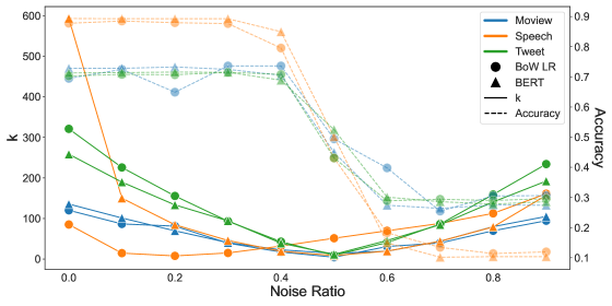
Figure 6: Average of $k=|\mathcal{S}_{t}|$ (solid line) and model’s accuracy (dashed line) for the test dataset with noise ratio from 0 to 0.9. When the noise ratio increases from 0 to 0.3, $k$ decreases apparently, while the model’s accuracy does not demonstrate a noticeable decline.

3.4 Composition of $\mathcal{S}_{t}$ Contributes Bias Explanation

Group attribution bias in machine learning refers to a model’s inclination to link specific attributes to a particular group, potentially resulting in biased predictions. We show that the integration of $\mathcal{S}_{t}$ is associated with group attribution biased in training data. As a case, we manually introduce group attribution bias into the loan default dataset Surana (2021), designed to predict potential defaulters for a consumer loan product. We augment a dataset containing basic consumer features with a manually added discrete "tag" feature, arbitrarily assigning 40% as "tag $X$" and 60% as "tag $Y$" We then introduce bias by relabeling 90% of the qualified "tag $X$" as "default." This biased set is defined as $\mathcal{B}$, where the wrong label tightly links with the feature "tag $X$." A logistic regression model is subsequently trained with this modified dataset.

We apply Algorithm 1 to misclassified test points and compute the proportion in each resulting subset $\mathcal{S}_{t}$ belonging to $\mathcal{B}$. The average proportions are 60% for "tag $X$" and 23% for "tag $Y$" misclassified data. The higher proportion in "tag $X$" suggests that the misclassification of eligible "tag $X$" individuals mainly results from the biased training set $\mathcal{B}$, whereas for "tag $Y$" individuals may be due to other reasons like model oversimplification. Thus, our approach can highlight training points contributing to group attribution bias.

3.5 Comparison between Removal and Relabeling

	Noisy points in $\mathcal{S}_{t1}$			Normal points in $\mathcal{S}_{t2}$
	Loan	Movie reviews	Speech	Loan	Movie reviews	Speech
Removal Alg1	47.9	1.8	146.8	30.6	2.1	31.9
Removal Alg2	45.6	1.8	104.2	27.0	2.1	21.0
Relabeling (ours)	11.6	0.8	55.8	22.9	1.3	8.2

Table 4: Average number of points to relabel and remove to flip a test prediction, categorized by noisy and normal points. Relabeling consistently leads to smaller sets of both noisy and normal points being altered.

In this section, we compare two ways to alter training points such that the alternation can result in the flipping of a test point: relabeling and removal. We show that the relabeling mechanism can reveal a smaller training subset, thus saving the cost of investigating suspicious training points.

Kong et al. (2021) firstly propose an algorithm to find the training subset to remove to flip a test prediction for economy models, which we denote as "Removal Alg1" in Table 7. Yang et al. (2023) employ the same algorithm on machine learning models and improve it to return a smaller training set, denoted as "Removal Alg2".

We aim to show that when noise is present in the training set, the relabeling mechanism consistently uncovers a smaller subset of influential points from the noisy training set while affecting fewer standard points. To demonstrate this, we introduced a 30% noise factor into the training set by flipping labels of normal points, denoted as $\mathcal{N}$, which increased misclassified test points. We identified the training set $\mathcal{S}_{t}$ using the three methods for these misclassified test points. We divided the identified training points $\mathcal{S}_{t}$ into two categories: training points belonging to the noise set $\mathcal{S}_{t1}=\mathcal{S}_{t}\cap\mathcal{N}$, and those that do not belong to the noise set $\mathcal{S}_{t2}=\mathcal{S}_{t}\setminus\mathcal{N}$. The results presented in Table 4 demonstrate that both the $S_{1}$ and $S_{2}$ subsets identified through the relabeling process are smaller than those identified through removal. This suggests that considering relabeling training points can more effectively discern fewer noisy and regular training points, saving the cost to investigate more suspicious points. We also show the conclusion holds when there is no noise in the training set in Sec A.2.

4 Related Work

The holding of model predictions. Several studies have explored the changes of a model behavior and its factors. Ilyas et al. (2022) analyzed model behavior changes based on different training data. Harzli et al. (2022) studied the change of a specific prediction by finding a smallest informative feature set to analize economy models. Additionally, research on counterfactual examples aims to explain predicted outcomes by identifying the feature values that caused the given prediction Kaushik et al. (2019). Recent studies investigated the influence function in machine learning to answer the question of "How many and which training points need to be removed to alter a specific prediction?" (Broderick et al., 2020; Yang et al., 2023). We follow these two works and propose an alternative way to alter the training points by asking, "How many and which training points would need to be relabeled to change this prediction?"

Trustworthy machine learning is important in today’s era, given the pervasive adoption of artificial intelligence systems in our everyday lives. Previous work emphasizes contestability as a key facet of trustworthiness, advocating for individuals’ right to challenge AI predictions (Vaccaro et al., 2019; Almada, 2019). This may involve providing evidence or alternative perspectives to challenge AI-derived conclusions (Hirsch et al., 2017). Our mechanism offers a way to draw upon training data as evidence when contest AI determination. In line with advancing model fairness, it’s crucial to address training data related to noise (Wang et al., 2018; Kuznetsova et al., 2020) and biases (Osoba and Welser IV, 2017; Howard and Borenstein, 2018). Our research shows that, despite different noise ratios, the model’s accuracy remains relatively consistent, yet there is a significant variation in the size of the subset $\mathcal{S}_{t}$. Furthermore, we demonstrate that in scenarios where group attribution bias is present, our method can aid in identifying the associated training points.

Influence function offers tools for identifying training data most responsible for a particular test prediction (Hampel, 1974; Cook and Weisberg, 1980, 1982). By uncovering mislabeled training points and/or outliers, influence can be used to debug training data and provide insight for the result generated by neural networks (Koh and Liang, 2017; Adebayo et al., 2020; Han et al., 2020; Pezeshkpour et al., 2022; Teso et al., 2021). Warnecke et al. (2021b) extend influence function to measure the influence of alternation in training points’ feature and label and apply it to machine unlearning. Furthermore, Kong et al. (2021) also extended influence on the effect of relabeling training points but utilized this measure to identify and recycle noisy training samples, leading to enhanced model performance at the training stage. Our research emphasizes utilizing this measure to determine which training subsets should be relabeled to question machine learning model predictions, and we delve into the factors influencing the integration and size of the identified subsets.

5 Discussion and Future Work

Extend the method to complex models. In today’s landscape dominated by large language models (LLMs), researchers are trying to integrate machine learning models into various decision-making processes, ranging from medical diagnoses (Shaib et al., 2023) to legal judgments (Jiang and Yang, 2023) and academic paper reviews (Liang et al., 2023). However, LLMs are black-box models and hard to explain despite their immense capabilities. They are prone to challenges including, but not limited to, social biases (Hutchinson et al., 2020; Bender et al., 2021; Abid et al., 2021; Weidinger et al., 2021; Bommasani et al., 2022) and the spread of misinformation (Evans et al., 2021; Lin et al., 2022). These immediate issues might be precursors to more profound, long-term risks for making decisions based on AI systems.

As we harness these models to make critical decisions, it becomes imperative to delve into the root causes of any erroneous determinations. As outlined in our research, our proposed method offers a pathway to trace the origins of such errors back to specific training data points. As the first to state this problem, we primarily focus on linear regression and BERT with a classifier. In the future, we envision our methodology applying to even more complex models. A recent study extends the influence function to LLMs to understand how training data alterations can impact model predictions (Grosse et al., 2023). Building upon this foundation, adapting our approach for LLMs is promising for future exploration. Because IP-relabel calculates how the predicted probability changes when training points are relabeled, we can readily adapt our method for multi-class tasks. If we know the desired label to which we want to change certain training points, we can simply adjust the threshold in Algorithm 1 to alter the test predictions accordingly.

Improve model performance. Instead of scaling up the number of datasets, we can focus on current data and alter them to improve the quality, enhancing downstream performance, as suggested by the reviewer. For instance, Kong et al. (2021) introduced a framework for relabeling incoming training points that may contain noise. This approach successfully improved the model’s performance on test data. Similarly, Teso et al. (2021) developed an algorithm to identify and eliminate potentially noisy training points, thereby improving the overall quality of the training set and, consequently, the model’s performance. Both studies utilized influence functions, a concept we employ, albeit with a distinct formulation as indicated in Equ. (4). Similarly, future work can consider enhancing the overall model performance by improving the data quality through identifying and relabeling training points that can flip wrong test predictions.

6 Conclusions

In this work, we introduce the problem of identifying a minimal subset of training data, $\mathcal{S}_{t}$, which, if relabeled before training, would result in a different test prediction. We propose a computationally efficient algorithm to address this task and evaluate its performance within binary classification models with convex loss. In the experiment, we illustrate that the size of the subset $|\mathcal{S}_{t}|$ can serve as a measure of the model and the training set’s robustness. Lastly, we indicate that the composition of $\mathcal{S}_{t}$ can reveal training points that cause group attribution bias.

7 Limitations and Risks

In our study, we’ve extensively used influence functions to solve the problem. However, being aware of fundamental limitations is crucial: they tend to be only effective in convex loss. The overarching goal of pinpointing a minimal subset within the training data, such that a change in labels leads to a reversal in prediction, isn’t exclusively achievable via approximations rooted in influence functions. This approach is favored in our work due to its intuitive nature and wide use. In addition, while Algorithm 1 currently shows less than optimal performance on the essay dataset, this presents an opportunity for further investigation. Specific characteristics unique to this dataset might influence the performance, opening up a valuable avenue for future research.

There exists an inherent risk wherein the same approach could be exploited to engender biased determinations. Specifically, by intentionally mislabeling genuine training data and subsequently retraining the model, actors with malicious intent might be able to invert just determinations, thereby compromising the model’s integrity and fairness. To counteract this risk, strategies such as regular data integrity checks, stringent access control, and employing model robustness techniques can be integrated, thereby ensuring the preservation of model authenticity and shielding against adversarial exploits.

Appendix A Appendix

A.1 Datasets and model details

We present basic statistics describing our text classification datasets in Table 5. We set the threshold for the hate speech data as 0.25 ($\tau=0.25$) to maximize the F1 score on the training set. For other datasets, we set the threshold as 0.5. For reference, we also report the hyperparameters and predictive performance realized by the models considered on the test sets of datasets in Table 6.

Dataset	# Train	# Test	% Pos
Loan	21120	2800	0.50
Movie reviews	6920	872	0.52
Essay	11678	1298	0.10
Hate speech	9632	1071	0.11
Tweet sentiment	18000	1000	0.50

Table 5: Dataset information.

Models	Accuracy	F1-score	AUC	l2
Loan
LR	0.79	0.80	0.88	100
Movie reviews
BoW	0.79	0.80	0.88	1000
BERT	0.82	0.83	0.91	500
Essay
BoW	0.97	0.80	0.99	1
BERT	0.98	0.87	0.99	10
Hate speech
BoW	0.87	0.40	0.81	10
BERT	0.89	0.63	0.88	10
Tweet sentiment
BoW	0.70	0.70	0.75	500
BERT	0.75	0.76	0.84	1000

Table 6: The model performance under different datasets.

A.2 Comparison between removal and relabeling on clean training set

When there is no noise in the training set, we run Removal Alg1, Removal Alg2, and Algorithm 1 to compare the average returned training set size in Table 7. It shows that considering training points to relabel can result in smaller training sets than removing them.

	Loan	Reviews	Speech
Removal Alg1	965.4	712.8	768.6
Removal Alg2	440.4	636.8	411.6
Relabeling (ours)	67.0	138.5	49.3

Table 7: The comparison of average on $k=|\mathcal{S}_{t}|$ values over a random subset of test points $x_{t}$, result by removal (Algorithm 1 and Algorithm 2 Yang et al. (2023)) and relabel. Relabel always finds a smaller $\mathcal{S}_{t}$ compared with removal.

A.3 Running time of Algorithm 1.

We recorded the average running time of Algorithm 1 to find $\mathcal{S}_{t}$ for test points in different datasets in Table 8 on Apple M1 Pro CPUs. For one test point, it just takes milliseconds to go through the whole training set (the training set sizes are provided in A.1) to find $\mathcal{S}_{t}$.

Dataset	BoW (ms)	BERT (ms)
Movie Reviews	19.04	140.51
Essays	160.01	265.09
Hate speech	103.70	299.46
Tweet	58.42	260.75
Loan	63.97	/

Table 8: Average running time (in milliseconds) of Algorithm 1 to find $\mathcal{S}_{t}$ for a test point in different datasets.

A.4 Full Plots

We present the distribution of $\mathcal{S}_{t}$ across various datasets in Tables 7 and 9. Additionally, the correlation between predicted probability and the size of $\mathcal{S}_{t}$, denoted by $|\mathcal{S}_{t}|$, for different datasets is showcased in Tables 8 and 10.

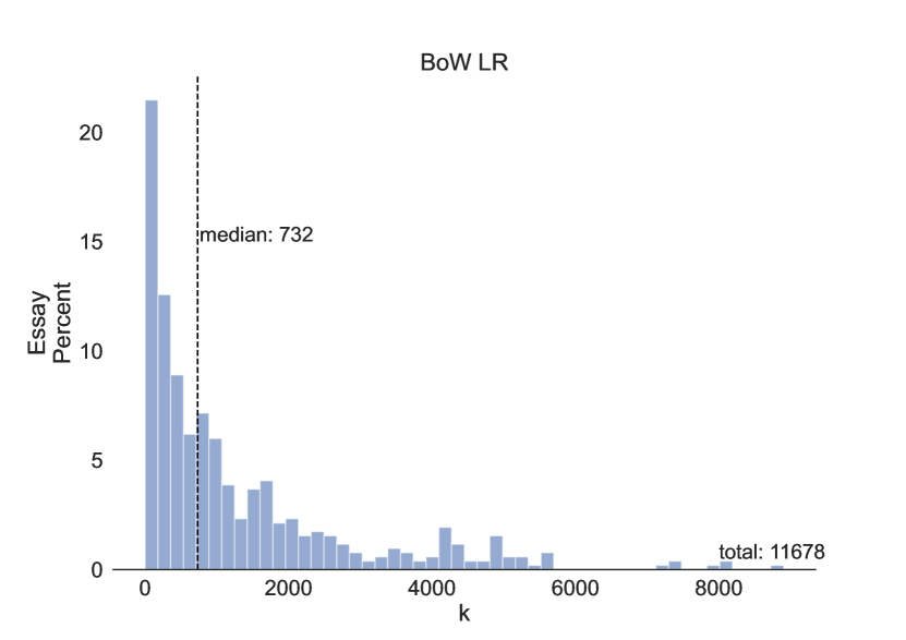
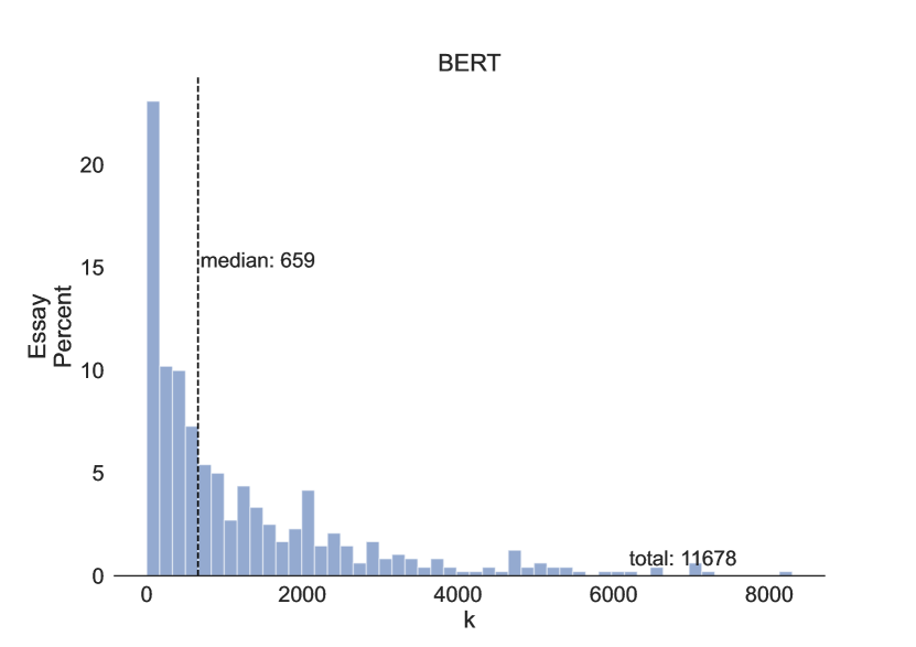
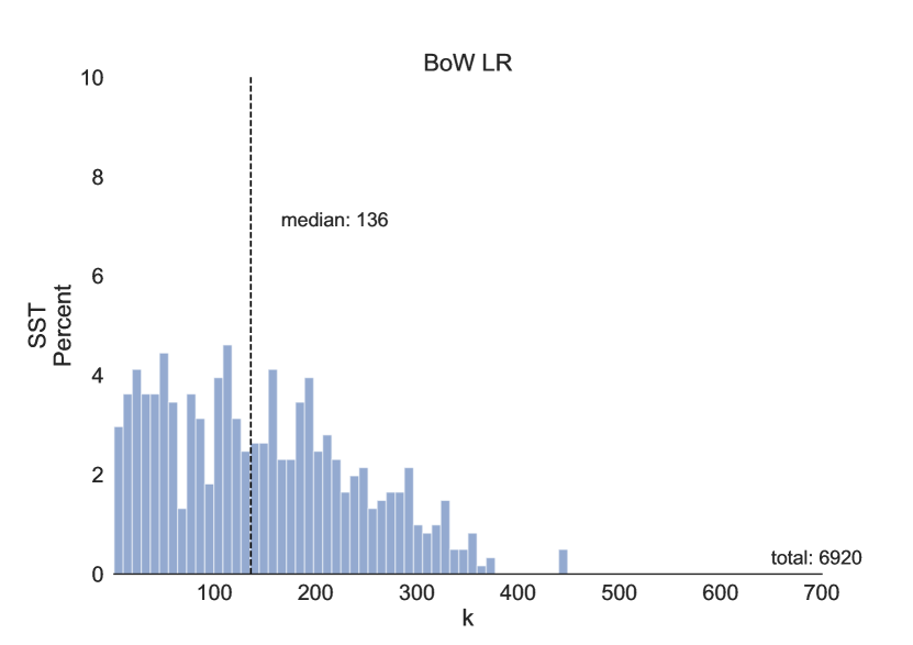
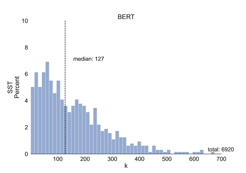
Figure 7: The histogram shows the distribution of $k=|\mathcal{S}_{t}|$, i.e. the number of points that need to be relabeled from the training data to change the prediction $\hat{y}_{t}$ of a specific test example $x_{t}$.

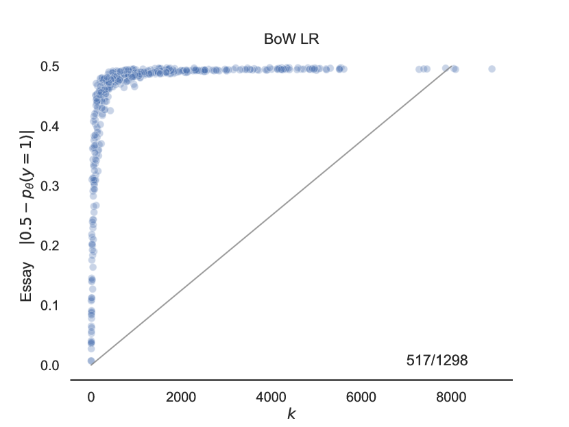
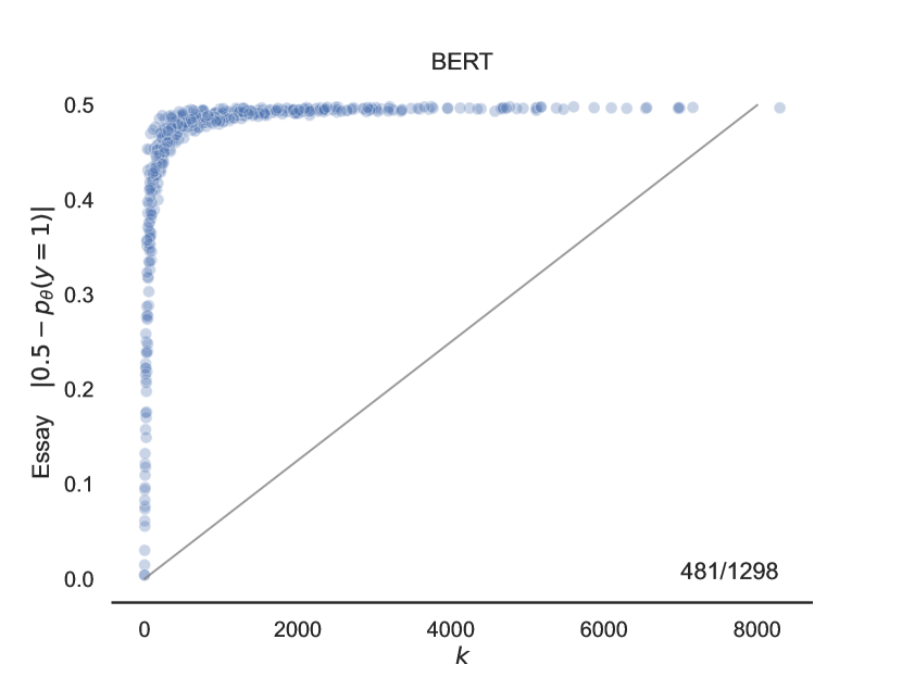
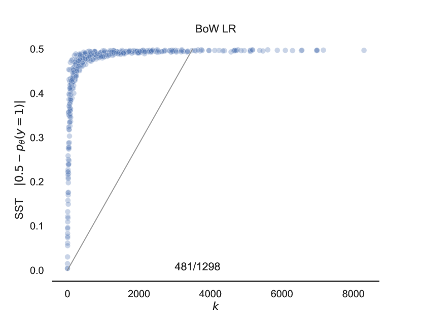
Figure 8: The plot displays the correlation between the predicted probabilities of certain test examples and $k=|\mathcal{S}_{t}|$ .There are some test examples where the model is reasonably or highly certain about its prediction, yet by removing a limited number of data points from the training set, the prediction can be altered.

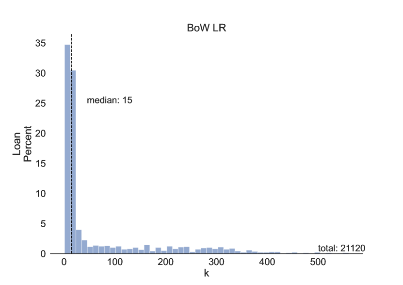
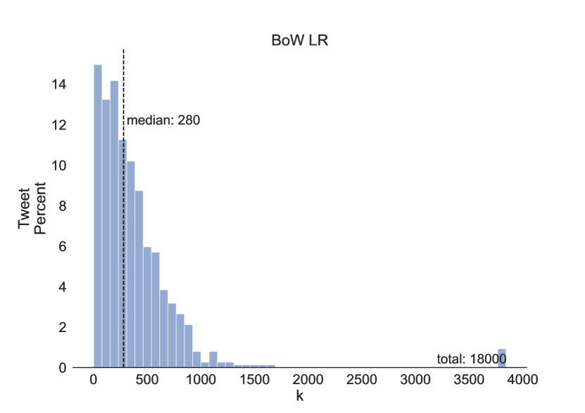
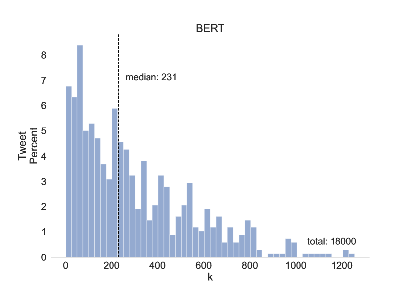
Figure 9: The histogram shows the distribution of $k=|\mathcal{S}_{t}|$, i.e. the number of points that need to be relabeled from the training data to change the prediction $\hat{y}_{t}$ of a specific test example $x_{t}$.

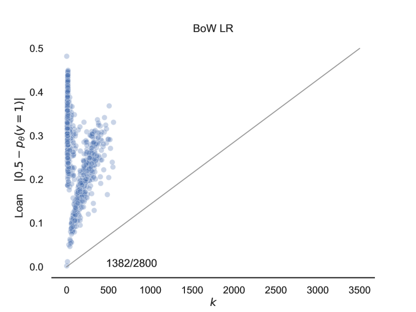
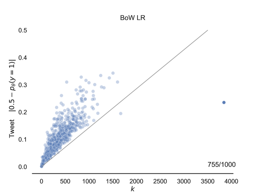
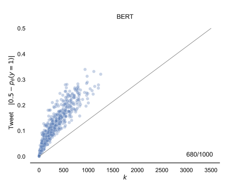
Figure 10: The plot displays the correlation between the predicted probabilities of certain test examples and $k=|\mathcal{S}_{t}|$ . Thethere are some test examples where the model is reasonably or highly certain about its prediction, yet by removing a limited number of data points from the training set, the prediction can be altered.

References

- Abid et al. (2021) Abubakar Abid, Maheen Farooqi, and James Zou. 2021. Persistent anti-muslim bias in large language models. In Proceedings of the 2021 AAAI/ACM Conference on AI, Ethics, and Society, pages 298–306.
- Adebayo et al. (2020) Julius Adebayo, Michael Muelly, Ilaria Liccardi, and Been Kim. 2020. Debugging tests for model explanations. arXiv preprint arXiv:2011.05429.
- Almada (2019) Marco Almada. 2019. Human intervention in automated decision-making: Toward the construction of contestable systems. In Proceedings of the Seventeenth International Conference on Artificial Intelligence and Law, pages 2–11.
- Barshan et al. (2020) Elnaz Barshan, Marc-Etienne Brunet, and Gintare Karolina Dziugaite. 2020. Relatif: Identifying explanatory training samples via relative influence. In International Conference on Artificial Intelligence and Statistics, pages 1899–1909. PMLR.
- Bender et al. (2021) Emily M Bender, Timnit Gebru, Angelina McMillan-Major, and Shmargaret Shmitchell. 2021. On the dangers of stochastic parrots: Can language models be too big? In Proceedings of the 2021 ACM conference on fairness, accountability, and transparency, pages 610–623.
- Bommasani et al. (2022) Rishi Bommasani, Drew A. Hudson, Ehsan Adeli, et al. 2022. On the opportunities and risks of foundation models.
- Broderick et al. (2020) Tamara Broderick, Ryan Giordano, and Rachael Meager. 2020. An automatic finite-sample robustness metric: When can dropping a little data make a big difference? arXiv preprint arXiv:2011.14999.
- Charpiat et al. (2019) Guillaume Charpiat, Nicolas Girard, Loris Felardos, and Yuliya Tarabalka. 2019. Input similarity from the neural network perspective. Advances in Neural Information Processing Systems, 32.
- Cook and Weisberg (1980) R Dennis Cook and Sanford Weisberg. 1980. Characterizations of an empirical influence function for detecting influential cases in regression. Technometrics, 22(4):495–508.
- Cook and Weisberg (1982) R Dennis Cook and Sanford Weisberg. 1982. Residuals and influence in regression. New York: Chapman and Hall.
- de Gibert et al. (2018) Ona de Gibert, Naiara Perez, Aitor García-Pablos, and Montse Cuadros. 2018. Hate Speech Dataset from a White Supremacy Forum. In Proceedings of the 2nd Workshop on Abusive Language Online (ALW2), pages 11–20, Brussels, Belgium. Association for Computational Linguistics.
- Devlin et al. (2018) Jacob Devlin, Ming-Wei Chang, Kenton Lee, and Kristina Toutanova. 2018. Bert: Pre-training of deep bidirectional transformers for language understanding. arXiv preprint arXiv:1810.04805.
- Evans et al. (2021) Owain Evans, Owen Cotton-Barratt, Lukas Finnveden, Adam Bales, Avital Balwit, Peter Wills, Luca Righetti, and William Saunders. 2021. Truthful ai: Developing and governing ai that does not lie.
- Foundation (2010) Hewlett Foundation. 2010. The hewlett foundation: Automated essay scoring.
- Go et al. (2009) Alec Go, Richa Bhayani, and Lei Huang. 2009. Twitter sentiment classification using distant supervision. CS224N project report, Stanford, 1(12):2009.
- Grosse et al. (2023) Roger Grosse, Juhan Bae, Cem Anil, Nelson Elhage, Alex Tamkin, Amirhossein Tajdini, Benoit Steiner, Dustin Li, Esin Durmus, Ethan Perez, Evan Hubinger, Kamilė Lukošiūtė, Karina Nguyen, Nicholas Joseph, Sam McCandlish, Jared Kaplan, and Samuel R. Bowman. 2023. Studying large language model generalization with influence functions.
- Hampel (1974) Frank R Hampel. 1974. The influence curve and its role in robust estimation. Journal of the american statistical association, 69(346):383–393.
- Han et al. (2020) Xiaochuang Han, Byron C Wallace, and Yulia Tsvetkov. 2020. Explaining black box predictions and unveiling data artifacts through influence functions. arXiv preprint arXiv:2005.06676.
- Harzli et al. (2022) Ouns El Harzli, Bernardo Cuenca Grau, and Ian Horrocks. 2022. Minimal explanations for neural network predictions. arXiv preprint arXiv:2205.09901.
- Hirsch et al. (2017) Tad Hirsch, Kritzia Merced, Shrikanth Narayanan, Zac E Imel, and David C Atkins. 2017. Designing contestability: Interaction design, machine learning, and mental health. In Proceedings of the 2017 Conference on Designing Interactive Systems, pages 95–99.
- Howard and Borenstein (2018) Ayanna Howard and Jason Borenstein. 2018. The ugly truth about ourselves and our robot creations: the problem of bias and social inequity. Science and engineering ethics, 24(5):1521–1536.
- Hutchinson et al. (2020) Ben Hutchinson, Vinodkumar Prabhakaran, Emily Denton, Kellie Webster, Yu Zhong, and Stephen Denuyl. 2020. Social biases in nlp models as barriers for persons with disabilities.
- Ilyas et al. (2022) Andrew Ilyas, Sung Min Park, Logan Engstrom, Guillaume Leclerc, and Aleksander Madry. 2022. Datamodels: Understanding predictions with data and data with predictions. In Proceedings of the 39th International Conference on Machine Learning, volume 162 of Proceedings of Machine Learning Research, pages 9525–9587. PMLR.
- Jiang and Yang (2023) Cong Jiang and Xiaolei Yang. 2023. Legal syllogism prompting: Teaching large language models for legal judgment prediction. In Proceedings of the Nineteenth International Conference on Artificial Intelligence and Law, pages 417–421.
- Kaushik et al. (2019) Divyansh Kaushik, Eduard Hovy, and Zachary C Lipton. 2019. Learning the difference that makes a difference with counterfactually-augmented data. arXiv preprint arXiv:1909.12434.
- Koh and Liang (2017) Pang Wei Koh and Percy Liang. 2017. Understanding black-box predictions via influence functions. In International conference on machine learning, pages 1885–1894. PMLR.
- Koh et al. (2019) Pang Wei W Koh, Kai-Siang Ang, Hubert Teo, and Percy S Liang. 2019. On the accuracy of influence functions for measuring group effects. Advances in neural information processing systems, 32.
- Kong et al. (2021) Shuming Kong, Yanyan Shen, and Linpeng Huang. 2021. Resolving training biases via influence-based data relabeling. In International Conference on Learning Representations.
- Kuznetsova et al. (2020) Alina Kuznetsova, Hassan Rom, Neil Alldrin, Jasper Uijlings, Ivan Krasin, Jordi Pont-Tuset, Shahab Kamali, Stefan Popov, Matteo Malloci, Alexander Kolesnikov, et al. 2020. The open images dataset v4. International Journal of Computer Vision, 128(7):1956–1981.
- Liang et al. (2023) Weixin Liang, Yuhui Zhang, Hancheng Cao, Binglu Wang, Daisy Ding, Xinyu Yang, Kailas Vodrahalli, Siyu He, Daniel Smith, Yian Yin, Daniel McFarland, and James Zou. 2023. Can large language models provide useful feedback on research papers? a large-scale empirical analysis.
- Lin et al. (2022) Stephanie Lin, Jacob Hilton, and Owain Evans. 2022. Truthfulqa: Measuring how models mimic human falsehoods.
- Marx et al. (2019) Charles Marx, Richard Phillips, Sorelle Friedler, Carlos Scheidegger, and Suresh Venkatasubramanian. 2019. Disentangling influence: Using disentangled representations to audit model predictions. Advances in Neural Information Processing Systems, 32.
- Osoba and Welser IV (2017) Osonde A Osoba and William Welser IV. 2017. An intelligence in our image: The risks of bias and errors in artificial intelligence. Rand Corporation.
- Pezeshkpour et al. (2022) Pouya Pezeshkpour, Sarthak Jain, Sameer Singh, and Byron Wallace. 2022. Combining feature and instance attribution to detect artifacts. In Findings of the Association for Computational Linguistics: ACL 2022, pages 1934–1946, Dublin, Ireland. Association for Computational Linguistics.
- Pezeshkpour et al. (2021) Pouya Pezeshkpour, Sarthak Jain, Byron C Wallace, and Sameer Singh. 2021. An empirical comparison of instance attribution methods for nlp. arXiv preprint arXiv:2104.04128.
- Shaib et al. (2023) Chantal Shaib, Millicent L Li, Sebastian Joseph, Iain J Marshall, Junyi Jessy Li, and Byron C Wallace. 2023. Summarizing, simplifying, and synthesizing medical evidence using gpt-3 (with varying success). arXiv preprint arXiv:2305.06299.
- Socher et al. (2013) Richard Socher, Alex Perelygin, Jean Wu, Jason Chuang, Christopher D Manning, Andrew Y Ng, and Christopher Potts. 2013. Recursive deep models for semantic compositionality over a sentiment treebank. In Proceedings of the 2013 conference on empirical methods in natural language processing, pages 1631–1642.
- Surana (2021) Ssubham Surana. 2021. Loan prediction based on customer behavior.
- Teso et al. (2021) Stefano Teso, Andrea Bontempelli, Fausto Giunchiglia, and Andrea Passerini. 2021. Interactive label cleaning with example-based explanations. Advances in Neural Information Processing Systems, 34:12966–12977.
- Vaccaro et al. (2019) Kristen Vaccaro, Karrie Karahalios, Deirdre K Mulligan, Daniel Kluttz, and Tad Hirsch. 2019. Contestability in algorithmic systems. In Conference Companion Publication of the 2019 on Computer Supported Cooperative Work and Social Computing, pages 523–527.
- Wang et al. (2018) Fei Wang, Liren Chen, Cheng Li, Shiyao Huang, Yanjie Chen, Chen Qian, and Chen Change Loy. 2018. The devil of face recognition is in the noise. In Proceedings of the European Conference on Computer Vision (ECCV), pages 765–780.
- Warnecke et al. (2021a) Alexander Warnecke, Lukas Pirch, Christian Wressnegger, and Konrad Rieck. 2021a. Machine unlearning of features and labels. arXiv preprint arXiv:2108.11577.
- Warnecke et al. (2021b) Alexander Warnecke, Lukas Pirch, Christian Wressnegger, and Konrad Rieck. 2021b. Machine unlearning of features and labels. arXiv preprint arXiv:2108.11577.
- Weidinger et al. (2021) Laura Weidinger, John Mellor, Maribeth Rauh, Conor Griffin, Jonathan Uesato, Po-Sen Huang, Myra Cheng, Mia Glaese, Borja Balle, Atoosa Kasirzadeh, Zac Kenton, Sasha Brown, Will Hawkins, Tom Stepleton, Courtney Biles, Abeba Birhane, Julia Haas, Laura Rimell, Lisa Anne Hendricks, William Isaac, Sean Legassick, Geoffrey Irving, and Iason Gabriel. 2021. Ethical and social risks of harm from language models.
- Yang et al. (2023) Jinghan Yang, Sarthak Jain, and Byron C Wallace. 2023. How many and which training points would need to be removed to flip this prediction? arXiv preprint arXiv:2302.02169.