The Decaying Missing-at-Random Framework: Doubly Robust Causal Inference with Partially Labeled Data

Abstract

In real-world scenarios, data collection limitations often result in partially labeled datasets, leading to difficulties in drawing reliable causal inferences. Traditional approaches in the semi-supervised (SS) and missing data literature may not adequately handle these complexities, leading to biased estimates. To address these challenges, our paper introduces a novel decaying missing-at-random (decaying MAR) framework. This framework tackles missing outcomes in high-dimensional settings and accounts for selection bias arising from the dependence of labeling probability on covariates. Notably, we relax the need for a positivity condition, commonly required in the missing data literature, and allow uniform decay of labeling propensity scores with sample size, accommodating faster growth of unlabeled data. Our decaying MAR framework enables easy rate double-robust (DR) estimation of average treatment effects, succeeding where other methods fail, even with correctly specified nuisance models. Additionally, it facilitates asymptotic normality under model misspecification. To achieve this, we propose adaptive new targeted bias-reducing nuisance estimators and asymmetric cross-fitting, along with a novel semi-parametric approach that fully leverages large volumes of unlabeled data. Our approach requires weak sparsity conditions. Numerical results confirm our estimators’ efficacy and versatility, addressing selection bias and model misspecification.

, and

T1All authors contributed equally in this work.

1 Introduction

Semi-supervised (SS) learning’s importance in estimating the average treatment effect (ATE) is increasingly recognized in a wide range of fields. Despite having a large total sample size (denoted as $N$), practical restrictions often result in missing outcomes (or labels) $Y\in\mathbb{R}$. The primary objective of this research is to explore how to effectively utilize this rich yet intricate dataset to study the causal impact of a binary treatment denoted as $T\in\{0,1\}$ on $Y$. For instance, in autonomous driving, exploiting abundant unlabeled camera footage could improve the detection of rare incidents. In the cybersecurity sector, the evaluation of extensive unlabeled data might enhance fraud detection capabilities. Wildlife conservation could benefit from using unlabeled images for population monitoring strategies. Similarly, integrative genomics studies can identify novel gene-disease associations by incorporating and analyzing large unlabeled datasets.

Under the potential outcome framework (Rubin, 1974; Imbens and Rubin, 2015), we consider potential outcomes $Y(0)$ and $Y(1)$, corresponding to treatment assignments $T=0$ and $T=1$, respectively. The observed outcome is denoted by $Y\equiv Y(T)$ and under consistency assumption $Y=TY(1)+(1-T)Y(0)$. The ATE characterizes the average causal effect of $T$ on $Y$ and is defined as

$$\mu_{0}:=\theta_{1}-\theta_{0},\;\;\text{where}\;\;\theta_{1}:=\mathbb{E}\{Y(1)\}\;\;\text{and}\;\;\theta_{0}:=\mathbb{E}\{Y(0)\}.$$ (1.1)

Estimating the ATE in observational studies, where the treatment $T$ and outcome $Y$ are influenced by a shared set of confounders $\mathbf{X}\in\mathbb{R}^{d}$, presents challenges due to confounding. The complexity deepens in semi-supervised (SS) settings. In this context, a labeled dataset $\mathcal{L}=(\mathbf{X}_{i},Y_{i})_{i=1}^{n}$ coexists with a substantial amount of unlabeled data $\mathcal{U}=(\mathbf{X}_{i})_{i=n+1}^{N}$, where the outcome variable is missing. Classical semi-supervised (SS) approaches assume that the labeled dataset ($\mathcal{L}$) and the unlabeled dataset ($\mathcal{U}$) share the same distribution, assuming missingness completely at random (MCAR) for the outcomes (Cheng, Ananthakrishnan and Cai, 2021; Zhang and Bradic, 2022; Hou, Mukherjee and Cai, 2021; Chakrabortty, Dai and Tchetgen, 2022). This assumption enables effective utilization of both labeled and unlabeled data. However, in real-world scenarios, MCAR is often violated. The objective of this paper is to address these limitations and tackle challenges associated with selection bias, where the missingness of the observed outcome $Y$, denoted as the labeling indicator $R$ $\in\{0,1\}$, is itself observational and possibly dependent on both $(T,\mathbf{X})$. Furthermore, in situations where the unlabeled dataset is much larger than the labeled dataset ($N\gg n$), the probability of observing $Y$ decreases as $N$ increases, which violates the positivity assumption (Crump et al., 2009).

1.1 Decaying MAR setup

Unlike ‘traditional’ SS settings, we treat $R$ as random here. We allow the labeled fraction $n/N>0$ to be arbitrarily close to zero, and study the theory when both $\mathbb{P}(R=1)\to 0$ and $N\to\infty$. Note that we consider the labeling probability $p_{N}:=\mathbb{P}(R=1)$, the marginal distribution of $R\equiv R_{(N)}$, as well as the conditional distribution of $R\mid(T,\mathbf{X})$ as (decaying) functions of $N$ and let $N\to\infty$; see Section 2 for the usefulness and necessity of this construction.

We define the true outcome regression (OR) models, the propensity score (PS) models corresponding to the treatment $T$ and the labeling indicator $R$, as well as the PS models for a ‘product’ indicator as follows. For $j\in\{0,1\}$ and $\mathbf{x}$ in $\mathcal{X}\subseteq\mathbb{R}^{d}$, the support of $\mathbf{X}$, we define:

$$\textbf{OR models:}\;\;m(j,\mathbf{x}):=\mathbb{E}\{Y(j)\mid\mathbf{X}=\mathbf{x}\}{\color[rgb]{0,0,0},}$$ (1.2)

$$\textbf{T-PS models:}\;\;\pi(\mathbf{x}):=\mathbb{P}(T=1\mid\mathbf{X}=\mathbf{x}),\;\;\pi(j,\mathbf{x}):=\mathbb{P}(T=j\mid R=1,\mathbf{X}=\mathbf{x}),$$ (1.3)

$$\textbf{R-PS models:}\;\;p_{N}(\mathbf{x}):=\mathbb{P}(R=1\mid\mathbf{X}=\mathbf{x}),\;\;p_{N}(j,\mathbf{x}):=\mathbb{P}(R=1\mid T=j,\mathbf{X}=\mathbf{x}),$$ (1.4)

$$\textbf{Product PS models:}\;\;\gamma_{N}(j,\mathbf{x})~{}:=~{}\mathbb{P}(\Gamma^{(j)}=1\mid\mathbf{X}=\mathbf{x}),\;\;\;{\color[rgb]{0,0,0}\mbox{and}\;\;\;\gamma_{N,j}:=\mathbb{P}(\Gamma^{(j)}=1)},$$ (1.5)

$${\color[rgb]{0,0,0}\mbox{where}\;\;\;\Gamma^{(1)}:=TR~{}~{}\mbox{and}~{}~{}\Gamma^{(0)}:=(1-T)R~{}~{}\mbox{are the {\it product indicators}.}}$$

Assumption 1 (Basic assumptions).

(a) We assume the ‘no unmeasured confounding’ (NUC) and overlap assumptions for the treatment $T$, so that for some constant $c\in(0,1/2)$:

$$T\mathchoice{\mathrel{\hbox to0.0pt{$\displaystyle\perp$\hss}\mkern 4.0mu{\displaystyle\perp}}}{\mathrel{\hbox to0.0pt{$\textstyle\perp$\hss}\mkern 4.0mu{\textstyle\perp}}}{\mathrel{\hbox to0.0pt{$\scriptstyle\perp$\hss}\mkern 4.0mu{\scriptstyle\perp}}}{\mathrel{\hbox to0.0pt{$\scriptscriptstyle\perp$\hss}\mkern 4.0mu{\scriptscriptstyle\perp}}}\{Y(0),Y(1)\}\mid\mathbf{X}\;\;\leadsto\mbox{({T-NUC})}\;\;\;\mbox{and}\;\;\;c<\pi(\mathbf{x})<1-c\;\;\forall\;\mathbf{x}\in\mathcal{X}\;\;\leadsto\mbox{({T-overlap})}.$$

(b) We further assume missing at random (MAR) condition and a ‘decaying overlap’ condition (DOC) for the labeling indicator $R\equiv R_{(N)}$ as follows:

$$R\mathchoice{\mathrel{\hbox to0.0pt{$\displaystyle\perp$\hss}\mkern 4.0mu{\displaystyle\perp}}}{\mathrel{\hbox to0.0pt{$\textstyle\perp$\hss}\mkern 4.0mu{\textstyle\perp}}}{\mathrel{\hbox to0.0pt{$\scriptstyle\perp$\hss}\mkern 4.0mu{\scriptstyle\perp}}}{\mathrel{\hbox to0.0pt{$\scriptscriptstyle\perp$\hss}\mkern 4.0mu{\scriptscriptstyle\perp}}}Y\mid(T,\mathbf{X})\;\;\leadsto\mbox{({R-MAR})};\;\;\;{\mbox{\color[rgb]{0,0,0}}and}\;\;\;\mbox{for any $\mathbf{x}\in\mathcal{X}$, $j\in\{0,1\}$, and for each fixed $N$},$$

$$\{p_{N}(\mathbf{x}),p_{N}(j,\mathbf{x})\}>0,\;\mbox{while possibly},\;\{p_{N}(\mathbf{x}),\;p_{N}(j,\mathbf{x})\}\rightarrow 0\;\mbox{as}\;N\rightarrow\infty\;\leadsto\mbox{({R-DOC}).}$$

The T-NUC assumption (‘ignorability’), and the T-overlap condition are commonly assumed (Rosenbaum and Rubin, 1983; Crump et al., 2009; Imbens and Rubin, 2015). The R-MAR condition was used recently in Wei et al. (2022), but the authors didn’t consider the full semi-supervised setting of $N\gg n$. Kallus and Mao (2020) discuss it but only develop theory under a relaxed case of $R\mathchoice{\mathrel{\hbox to0.0pt{$\displaystyle\perp$\hss}\mkern 4.0mu{\displaystyle\perp}}}{\mathrel{\hbox to0.0pt{$\textstyle\perp$\hss}\mkern 4.0mu{\textstyle\perp}}}{\mathrel{\hbox to0.0pt{$\scriptstyle\perp$\hss}\mkern 4.0mu{\scriptstyle\perp}}}{\mathrel{\hbox to0.0pt{$\scriptscriptstyle\perp$\hss}\mkern 4.0mu{\scriptscriptstyle\perp}}}T\mid\mathbf{X}$ with a troublesome assumption $\mathbb{P}(R=1)=0$, which leads to $n=\sum_{i=1}^{N}R_{i}=0$ almost surely, i.e., a degenerate unsupervised setting. For this, the R-DOC assumption plays a critical role and is a non-standard condition. It is weaker than the traditional positivity condition, which requires the existence of a constant $c>0$ independent of $N$ such that $p_{N}(\mathbf{x})>c$ (and $p_{N}(j,\mathbf{x})>c$ in causal setups) (Bang and Robins, 2005; Tsiatis, 2007). Recently, Zhang, Chakrabortty and Bradic (2023) considered a slightly different version of the R-DOC condition that only involves conditions for $p_{N}(\cdot)$. When both the R-MAR and R-DOC conditions are satisfied, we refer to it as the ‘decaying MAR setting’.

1.2 Our contributions

We introduce a decaying MAR setting, redefining the non-MCAR SS setup. This transformative approach addresses a previously uncharted intersection: it tackles the often-ignored selection bias in the SS literature and challenges the traditional positivity condition in the missing data domain; see Table 1.1. By doing so, our research contributes to the literature on the ‘generalizability’ of randomized controlled trials (RCTs), where RCT is combined with unlabeled, external data; see Dahabreh et al. (2019), Lesko et al. (2017) and also Shi, Pan and Miao (2023) for a review. In our context, $R$ denotes whether an individual is involved in the RCT or not and lack of strict positivity condition allows our work to be impactful when external data size surpasses that of an RCT.

Table 1.1: Comparison of the missing outcome settings. ‘Selection bias’ allows $R$ to be dependent on $(Y,\mathbf{X})$. ‘Causal setup $+$ missing $Y$’ allows for the observed outcome $Y=Y(T)$ to be possibly missing with $R,T\not\equiv 1$.

Settings	Selection	Decaying	Causal $+$
	Bias	PS	missing $Y$
Kawakita and Kanamori (2013); Azriel et al. (2022); Chakrabortty and Cai (2018); Zhang, Brown and Cai (2019); Cai and Guo (2020); Chan et al. (2020); Xue, Ma and Li (2021); Chakrabortty, Dai and Carroll (2022)	$\times$	$\checkmark$	$\times$
Cheng, Ananthakrishnan and Cai (2021); Hou, Mukherjee and Cai (2021); Zhang and Bradic (2022); Chakrabortty, Dai and Tchetgen (2022)	$\times$	$\checkmark$	$\checkmark$
Rubin (1976); Robins, Rotnitzky and Zhao (1994); Robins and Rotnitzky (1995); Bang and Robins (2005); Tsiatis (2007); Kang and Schafer (2007); Graham (2011); Chakrabortty et al. (2019)	$\checkmark$	$\times$	$\times$
Dahabreh et al. (2019); Lesko et al. (2017); Kallus and Mao (2020); Wei et al. (2022)	$\checkmark$	$\times$	$\checkmark$
Zhang, Chakrabortty and Bradic (2023)	$\checkmark$	$\checkmark$	$\times$
The proposed (causal) decaying MAR setting	$\checkmark$	$\checkmark$	$\checkmark$

As we improve DR properties, understanding their definitions is crucial. The model DR property states that the ATE estimator is asymptotically normally distributed when either of the nuisances is correctly specified. See Tan (2020) and Dukes, Avagyan and Vansteelandt (2020), with minor modifications in Smucler, Rotnitzky and Robins (2019). The rate DR property requires both nuisances to be correctly specified with the product of their sparsities of the order of $o(N)$. The sparsity DR property of Bradic, Wager and Zhu (2019), needs correct model specifications with one ultra-sparse nuisance at $o(\sqrt{N})$, while the other is at $o(N)$ for PS with ultra-sparse OR, or $o(N^{3/4})$ for the OR with ultra-sparse PS.

We highlight the utility of decaying MAR framework by discussing the ease of attaining rate DR; see (A.7) and Theorem A.2 with adaptive rates accounting for PS decay. Prior research, even those based on simpler MCAR conditions or neglecting $N\gg n$ scenarios, has been limited; see Remark 1. Decaying MAR extends to missing treatment cases as well; see Corollary 3.1. We then propose two new DR method classes, each anchored in distinct PS representations. The first is parametric, introducing the sparsity DR and model DR bias-reduced doubly robust decaying MAR (DR-DMAR) SS estimator, abbreviated as BRSS (Section 4.1). The second approach is semi-parametric, named the semi-parametric bias-reduced DR-DMAR SS estimator (abbreviated as SP-BRSS, see Section 4.3). This approach takes advantage of the fully observed pairs $(T_{i},\mathbf{X}_{i})$ and advances a broader range of sparsity DR and model DR robust techniques with a new nuisance model class. Our primary findings are Theorems 4.4, 4.5, and Corollary 4.6. Our method, subsumes existing (special) cases: Chernozhukov et al. (2018)’s rate DR method with $R\equiv 1$, Zhang and Bradic (2022) and Chakrabortty, Dai and Tchetgen (2022) DR method under a consistent PS of $n/N$, and Zhang, Chakrabortty and Bradic (2023)’s non-causal DR with $T\equiv 1$; see Remark 3. We however, exhibit better robustness and outperform these methods, even in the canonical cases, as evidenced in Figure 1 and Table 4.1.

1.3 Organization

Section 2 introduces the decaying MAR setting and ATE’s identification. Section 3 proposes the DR-DMAR SS estimator and its theoretical properties. Sections 3.2 and 3.3 discuss decaying PS estimation and missing treatments. Section 4 defines a BRSS estimator with a parametric and a semi-parametric approaches and showcases main theoretical results. Sections 5 and 6 provide numerical results on simulated and pseudo-random datasets. Concluding discussion is in Section 7 whereas additional results, and the proofs are relegated to the Supplement.

1.4 Notation

Throughout this work we will use various positive constants independent of $N$ denoted as lower or capital letters $c$ and $C$. $\mathbb{P}(\cdot)$ and $\mathbb{E}(\cdot)$ indicate the joint distribution and expectation of random vector $\mathbb{Z}$. $\mathbb{P}_{\mathbf{X}}$ and $\mathbb{E}_{\mathbf{X}}\{f(\mathbf{X})\}$ denote the marginal distribution of $\mathbf{X}$ and expectation for any function $f$, respectively. For any subset $\mathcal{A}$, $\mathbb{P}_{\mathcal{A}}$ and $\mathbb{E}_{\mathcal{A}}(\cdot)$ signify its joint distribution and respective expectation. For any $r>0$, $\|f(\cdot)\|_{\mathbb{P},r}:=\{\mathbb{E}|f(\mathbb{Z})|^{r}\}^{1/r}$ and for any vector $\mathbf{z}\in\mathbb{R}^{d}$, $\|\mathbf{z}\|_{r}:=(\sum_{j=1}^{d}|\mathbf{z}_{j}|^{r})^{1/r}$, $\|\mathbf{z}\|_{0}:=|\{j:\mathbf{z}_{j}\neq 0\}|$, and $\|\mathbf{z}\|_{\infty}:=\max_{j}|\mathbf{z}_{j}|$. For any square matrix $\bm{\Sigma}\in\mathbb{R}^{d\times d}$, $\|\bm{\Sigma}\|_{r}:=\sup_{\color[rgb]{0,0,0}\|\mathbf{v}\|\neq 0}\|\bm{\Sigma}\mathbf{v}\|_{r}/\|\mathbf{v}\|_{r}$. $a_{N}\asymp b_{N}$ denotes equivalent sequences. Lastly, $\mathbf{e}_{j}\in\mathbb{R}^{d}$ refers to the $j$-th column of identity matrix $\mathbbm{I}_{d}\in\mathbb{R}^{d\times d}$.

2 The decaying MAR setting and estimation of the ATE

In the context of SS inference assuming MCAR, the goal is to improve the supervised approach’s efficiency using unlabeled data. However, in a decaying MAR framework, this becomes invalid, and MCAR-based methods introduce bias. Hence, we face a more challenging task: addressing identification issues from scratch to achieve consistent, optimal, and efficient SS estimation within a non-standard asymptotic regime.

Necessity and usefulness of the decaying PS

One primary contribution of this paper is the introduction of the decaying MAR schema, which addresses the dependence of $p_{N}$, $p_{N}(\mathbf{X})$, $R\equiv R_{(N)}$, and $R\mid(T,\mathbf{X})$ on $N$ and $\mathbf{X}$ in $N\gg n$ semi-supervised (SS) contexts. This schema accounts for the asymptotic scenario where $N\to\infty$ and $\mathbb{P}(R=1)\to 0$. Previous studies may have overlooked this aspect, leading to limitations in exploring the crucial $N\gg n$ setting and only allowing $\mathbb{P}(R=1)=c=\lim_{N\to\infty}n/N>0$. In conventional doubly-robust (DR) literature, estimation error control relies on $p_{N}^{-2}\|\widehat{\bm{\alpha}}-\bm{\alpha}^{*}\|_{2}=o(1)$ for a nuisance parameter $\bm{\alpha}^{*}$ and its corresponding estimator $\widehat{\bm{\alpha}}$; see, e.g., the control of $\mathcal{I}_{2}$ in Step 5 of the proof of Theorems 5.1 and 5.2 of Chernozhukov et al. (2018). However, this condition becomes excessively demanding when $p_{N}\to 0$, rendering accurate estimation of the nuisance parameters practically unattainable. For instance, as the expected labeled sample size is only $\mathbb{E}(n)=Np_{N}$, we have $\|\widehat{\bm{\alpha}}-\bm{\alpha}^{*}\|_{2}=O_{p}((Np_{N})^{-1/2})$ even in low dimensions. This leads to a very restrictive requirement on the decaying probability, $Np_{N}^{5}\to\infty$. Through refined analysis on the decaying PS, our results only require $\mathbb{E}(n)=Np_{N}\to\infty$.

Identification of the parameter(s)

Given definitions in (1.2)-(1.4) and Assumption 1, we identify multiple versions of our parameters, each with unique benefits and interpretations and involving estimable nuisance functions from observed data. These include conditional mean regression (Reg.), inverse probability weighting (IPW) with propensity score (PS) modeling, and augmented IPW representations that use both the conditional mean and PS. We illustrate these for $\theta_{1}=\mathbb{E}\{Y(1)\}$ without loss of generality, with analogous versions for $\theta_{0}=\mathbb{E}\{Y(0)\}$ by substituting $(T,Y(1))$ with $(1-T,Y(0))$. To simplify the notation, we let

$$\Gamma:=\Gamma^{(1)},\;\;\gamma_{N}:=\gamma_{N,1},\;\;\gamma_{N}(\cdot):=\gamma_{N}(1,\cdot),\;\;{\color[rgb]{0,0,0}\mbox{and}}\;\;m(\cdot):=m(1,\cdot).$$

Lemma 2.1 (Identification of $\theta_{1}$).

Let Assumption 1 hold. Then, we have the following Reg. and IPW representations (Rep.):

$$\theta_{1}~{}=~{}\mathbb{E}\left\{m(\mathbf{X})\right\}\;\;\leadsto\;\mbox{({\emph{Reg. Rep.}})},\quad\theta_{1}~{}=~{}\mathbb{E}\left\{\frac{\Gamma Y}{\gamma_{N}(\mathbf{X})}\right\}\;\;\leadsto\;\mbox{({\emph{IPW Rep.}})},$$

where $m(\cdot)$ is identifiable as $m(\mathbf{x})=\mathbb{E}(Y\mid\mathbf{X}=\mathbf{x},\Gamma=1)$. Additionally, for any arbitrary functions $m^{*}(\cdot)$ and $\gamma_{N}^{*}(\cdot)$, as long as either $m^{*}(\cdot)=m(\cdot)$ or $\gamma_{N}^{*}(\cdot)=\gamma_{N}(\cdot)$ holds but not necessarily both, we have:

$$\mathbb{E}\left\{\psi^{*}_{N,1}(\mathbf{Z})\right\}=0\;\;\leadsto\;\mbox{({\emph{DR Rep.}})},\mbox{ with }\psi^{*}_{N,1}(\mathbf{Z})=m^{*}(\mathbf{X})-\theta_{1}+\frac{\Gamma}{\gamma_{N}^{*}(\mathbf{X})}\left\{Y-m^{*}(\mathbf{X})\right\}.$$ (2.1)

The aforementioned representations elucidate that this can be seen as a mean estimation issue with a MAR labeling, with the effective labeling indicator being $\Gamma=TR$. The DR representation tolerates misspecification in $m(\cdot)$ or $\gamma_{N}(\cdot)$, resulting in a consistent $\theta_{1}$ estimator if either, but not necessarily both, are correctly estimated.

3 The general DR-DMAR SS ATE estimator: construction and asymptotics

We split the samples into $\mathbb{K}\geq 2$ parts, $\mathcal{I}_{1},\dots,\mathcal{I}_{\mathbb{K}}$ of equal sizes $|\mathcal{I}_{k}|=M=N/\mathbb{K}$ and define $\mathcal{I}_{-k}=\mathcal{I}\setminus\mathcal{I}_{k}$, $\forall k\leq\mathbb{K}$. Let $\widehat{m}^{(-k)}(j,\cdot)$ and $\widehat{\gamma}_{N}^{(-k)}(j,\cdot)$ be estimators of $m(j,\cdot)$ and $\gamma_{N}(j,\cdot)$, respectively, using the samples from $\mathcal{I}_{-k}$, based on suitable (working) models with one but not necessarily both required to be correctly specified. The estimator $\widehat{\gamma}_{N}(\cdot)=\widehat{\gamma}_{N}(1,\cdot)$ can be obtained in multiple ways: directly modelling $\Gamma\mid\mathbf{X}\equiv TR\mid\mathbf{X}$ or modeling $T\mid\mathbf{X}$ and $R\mid(T=1,\mathbf{X})$ or by modeling $R\mid\mathbf{X}$ and $T\mid(R=1,\mathbf{X})$; see more discussions in Section 3.2. The estimator $\widehat{m}(\cdot)=\widehat{m}(1,\cdot)$, on the other hand, can be simply obtained via any suitable (working) regression model for $(Y\mid T=1,R=1,\mathbf{X})\equiv(Y\mid TR=1,\mathbf{X})$. For each $i\in\mathcal{I}_{k}$, $\widetilde{m}(j,\mathbf{X}_{i})=\widehat{m}^{(-k)}(j,\mathbf{X}_{i})$ and $\widetilde{\gamma}_{N}(j,\mathbf{X}_{i})=\widehat{\gamma}_{N}^{(-k)}(j,\mathbf{X}_{i})$. We now define our DR decaying MAR (DR-DMAR) SS estimator $\widehat{\theta}_{j,\SS}$ of $\theta_{j}$ ($j\in\{0,1\}$) as

$$\widehat{\theta}_{j,\SS}\;:=\;\frac{1}{N}\sum_{i=1}^{N}\widetilde{m}(j,\mathbf{X}_{i})+\frac{\Gamma_{i}^{(j)}(Y_{i}-\widetilde{m}(j,\mathbf{X}_{i}))}{\widetilde{\gamma}_{N}(j,\mathbf{X}_{i})},$$ (3.1)

where $\Gamma_{i}^{(1)}:=T_{i}R_{i}$ and $\Gamma_{i}^{(0)}:=(1-T_{i})R_{i}$. The DR-DMAR SS ATE estimator is defined as:

$$\widehat{\mu}_{\SS}:=\widehat{\theta}_{1,\SS}-\widehat{\theta}_{0,\SS}.$$ (3.2)

3.1 Asymptotic properties

Let $\gamma^{*}_{N}(j,\cdot)=\gamma_{N}(j,\cdot)$ and $m^{*}(j,\cdot)=m(j,\cdot)$. The Supplement’s Theorems A.2-A.3 provide a full description of the main and supporting results; see Supplement. Here, we emphasize conclusions and their significance. Assume $\mathbb{E}\{\gamma_{N}^{-1}(j,\mathbf{X})\}<\infty$ and define

$$a_{N,j}:=[\mathbb{E}\{\gamma_{N}^{-1}(j,\mathbf{X})\}]^{-1}\;\;\mbox{and}\;\;a_{N}:=\min(a_{N,1},a_{N,0}).$$

For each $j\in\{0,1\}$, define the DR score

$$\psi_{N,j}^{opt}(\mathbf{Z}) \;:=\;m(j,\mathbf{X})-\theta_{j}+\frac{\Gamma^{(j)}}{\gamma_{N}(j,\mathbf{X})}\{Y(j)-m(j,\mathbf{X})\}.$$

Under the listed full conditions in the Supplement and with the product rate condition satisfied for each $j\in\{0,1\}$,

$$\mathbb{E}_{\mathbf{X}}\{\widehat{m}(j,\mathbf{X})-m(j,\mathbf{X})\}^{2}\mathbb{E}_{\mathbf{X}}\left\{1-\frac{\gamma_{N}(j,\mathbf{X})}{\widehat{\gamma}_{N}(j,\mathbf{X})}\right\}^{2}:=O_{p}(c_{N,j}^{2}d_{N,j}^{2})=o_{p}(1/(Na_{N})),$$ (3.3)

the DR-DMAR SS estimator is rate DR in that

$$\sqrt{Na_{N}}(\widehat{\mu}_{\SS}-\mu_{0})=O_{p}(1)\;\;\mbox{and}\;\;\sqrt{N}\left(\Sigma^{opt}_{N}\right)^{-1/2}(\widehat{\mu}_{\SS}-\mu_{0})\xrightarrow{d}\mathcal{N}(0,1),$$ (3.4)

where $\Sigma_{N}^{opt}:=\mbox{Var}\{\psi^{opt}_{N,1}(\mathbf{Z})-\psi^{opt}_{N,0}(\mathbf{Z})\}\asymp a_{N}^{-1}$. Here, $Na_{N}$ denotes the ‘effective sample size’ within a decaying MAR context, while $a_{N}$ signifies the deceleration factor resulting from the decaying PS, giving rise to atypical convergence rates. A simpler non-causal problem was studied in Zhang, Chakrabortty and Bradic (2023). In causal scenarios, Kallus and Mao (2020) proposed a rate DR theory for the ATE, setting semi-parametric efficiency bounds for possible missing outcomes and observable surrogate variables. However, their modeling is founded in a critically flawed $\mathbb{P}(R=1)=0$ (see discussion in Section 1.1) and their Theorems 4.1 and 4.2 rely on $R\mathchoice{\mathrel{\hbox to0.0pt{$\displaystyle\perp$\hss}\mkern 4.0mu{\displaystyle\perp}}}{\mathrel{\hbox to0.0pt{$\textstyle\perp$\hss}\mkern 4.0mu{\textstyle\perp}}}{\mathrel{\hbox to0.0pt{$\scriptstyle\perp$\hss}\mkern 4.0mu{\scriptstyle\perp}}}{\mathrel{\hbox to0.0pt{$\scriptscriptstyle\perp$\hss}\mkern 4.0mu{\scriptscriptstyle\perp}}}T\mid\mathbf{X}$ which we remove. Yet our result achieves their semi-parametric efficiency bound.

Remark 1 (Comparing with Special Cases of Decaying MAR Studies).

In the supervised causal setting, $Y$ is always observable ($R\equiv 1$). Our findings in (A.7) (and Theorem A.2) are in line with but are distinct from those of double machine learning (Chernozhukov et al., 2018); directly adopting their result would lead to sub-optimal convergence rates. For accuracy, we control the non-standard ratio $\Gamma_{i}^{(j)}/\widetilde{\gamma}_{N}(j,\mathbf{X}_{i})$ of (3.1) where most $\Gamma_{i}^{(j)}$ are zeros, and $\widetilde{\gamma}_{N}(j,\mathbf{x})$ may decay uniformly over $\mathbf{x}\in\mathcal{X}$. A low-dimensional DR solution of Wei et al. (2022) uses strict positivity condition ($p_{N}>c>0$) which forbids a truly SS setting where $N\gg n$. The regular SS setup includes MCAR-missing outcomes only (Cheng, Ananthakrishnan and Cai, 2021; Zhang, Brown and Cai, 2019; Hou, Mukherjee and Cai, 2021). The ATE estimators of Zhang and Bradic (2022); Chakrabortty, Dai and Tchetgen (2022) are special case of ours, but exhibit bias when missingness is not completely at random.

3.2 Estimation of the PS

Estimating PS in the decaying MAR setting is challenging due to extreme imbalance: the proportion of the labeled group relative to the full data size becomes exceptionally small. However, the decaying MAR provides three representations of the $\gamma_{N}(j,\cdot)$ function, enhancing flexibility in model formulation, robustness, and theoretical prerequisites. For simplicity, we consider $a_{N,1}\asymp a_{N,0}\asymp a_{N}\to 0$. The PS function $\gamma_{N}(\cdot)=\gamma_{N}(1,\cdot)$ can be represented as

$$\gamma_{N}(\cdot)=\mathbb{P}(\Gamma=1\mid\cdot)\;\;\mbox{ or }\;\;\gamma_{N}(\cdot)=\pi(1,\cdot)p_{N}(\cdot)\;\;\mbox{ or }\;\;\gamma_{N}(\cdot)=\pi(\cdot)p_{N}(1,\cdot).$$

We will explore each case individually, assuming a linear OR model with a slope of sparsity $s_{\bm{\alpha},1}$, and a Lasso estimate resulting in $c_{N,1}\asymp\sqrt{s_{\alpha,1}\log d/(Na_{N})}$ of (3.3).

Model 1: a logistic $\gamma_{N}(\cdot)$

This setting is especially suitable when the treatment and labeling indicators, $T$ and $R$, are affected by the same set of covariates. Here $\gamma_{N}(\mathbf{x})$ is modeled directly as a logistic function with a diverging offset:

$$\gamma_{N}(\mathbf{x})~{}=~{}\frac{\gamma_{N}\exp(\mathbf{x}^{T}\bm{\beta})}{1+\gamma_{N}\exp(\mathbf{x}^{T}\bm{\beta})}~{}=~{}\frac{\exp(\mathbf{x}^{T}\bm{\beta}+\log\gamma_{N})}{1+\exp(\mathbf{x}^{T}\bm{\beta}+\log\gamma_{N})},\;\;\forall\mathbf{x}\in\mathcal{X},$$ (3.5)

where $\bm{\beta}\in\mathbb{R}^{d}$ and the decaying nature of the PS function is captured by the diverging ‘offset’ term $\log\gamma_{N}$ where $\gamma_{N}:=\mathbb{E}(\Gamma)\to 0$ as $N$ grows. Zhang, Chakrabortty and Bradic (2023) considered the offset-based logistic model to capture $p_{N}(\mathbf{X})=\mathbb{P}(R=1\mid\mathbf{X})$ in non-causal contexts. Under conditions of Theorem 4.2 and Lemma 4.3 therein, an offset estimator above satisfies Assumptions 8, 9, and 10 with $a_{N}\asymp\gamma_{N}$, $d_{N,1}\asymp\sqrt{s_{\beta,1}\log d/(Na_{N})}$ (see (3.3)), and $s_{\beta,1}:=\|\bm{\beta}\|_{0}$. implying the ‘product-rate’ condition: $s_{\bm{\alpha},1}s_{\bm{\beta},1}=o(Na_{N}/{\log^{2}d})$.

Model 2: a logistic $p_{N}(1,\cdot)$ and a non-parametric $\pi(\cdot)$

Model 2 is preferable when distinct covariates influence $T$ and $R$, especially if only a fraction affects $R$. We propose a semi-parametric approach, modeling $\gamma_{N}(\mathbf{x})=\pi(\mathbf{x})p_{N}(1,\mathbf{x})$. Here, $\pi(\mathbf{X})$ is non-parametrically representing $P(T=1|\mathbf{X})$, and $p_{N}(1,\mathbf{X})=P(R=1|T=1,\mathbf{X})$ is modeled as an offset-based logistic function parameterized by $\bm{\beta}_{p,1}\in\mathbb{R}^{d}$:

$$p_{N}(1,\mathbf{x})=\frac{p_{N,1}\exp(\mathbf{x}^{T}\bm{\beta}_{p,1})}{1+p_{N,1}\exp(\mathbf{x}^{T}\bm{\beta}_{p,1})},\;\;\forall\mathbf{x}\in\mathcal{X},$$ (3.6)

where $p_{N,1}:=\mathbb{E}\{p_{N}(1,\mathbf{X})\}\asymp\gamma_{N}$ decays to zero with growing $N$. In this semi-parametric approach, we exploit the entire dataset, including both labeled and unlabeled samples denoted as $N$, to estimate $\pi(\cdot)$. In contrast, the estimation error of $p_{N}(1,\cdot)$ is controlled by the rate $Na_{N}$, considerably smaller than $N$ as per the decaying MAR with $a_{N}\to 0$ as $N$ grows. For example, an optimally tuned random forest yields an estimation error $O_{p}(N^{-1/(11.1\alpha_{1}\lor 16.1)})$ for some $\alpha_{1}>0$ (Chi et al., 2022). With the estimation error of $p_{N}(1,\cdot)$ being $O_{p}(\sqrt{s_{p,1}\log d/(Na_{N})})$, with $s_{p,1}=\|\bm{\beta}_{p,1}\|_{0}$, whenever $a_{N}\ll s_{p,1}N^{2/(11.1\alpha_{1}\lor 16.1)-1}\log d$, the non-parametric error of $\pi(\cdot)$ is of smaller order than $p_{N}(1,\cdot)$, resulting in a ‘product-rate’ condition of $s_{\bm{\alpha},1}s_{p,1}=o(Na_{N}/{\log^{2}d})$ arises. In Section 4.3 below, we will revisit and refine the approach here and provide ATE inference even under model misspecification along with weaker sparsity conditions.

Model 3: a logistic $p_{N}(\cdot)$ and a logistic $\pi(1,\cdot)$

In the data integration context, we generalize causal inference from randomized trials to a broader population containing both clinical trial data, where outcome $Y$ is observed, and non-randomized data with missing $Y$. Randomization indicator $R$ is confounded by $\mathbf{X}$, and treatment $T$ is often assigned after $R$. We propose alternative identification assumptions: $R\mathchoice{\mathrel{\hbox to0.0pt{$\displaystyle\perp$\hss}\mkern 4.0mu{\displaystyle\perp}}}{\mathrel{\hbox to0.0pt{$\textstyle\perp$\hss}\mkern 4.0mu{\textstyle\perp}}}{\mathrel{\hbox to0.0pt{$\scriptstyle\perp$\hss}\mkern 4.0mu{\scriptstyle\perp}}}{\mathrel{\hbox to0.0pt{$\scriptscriptstyle\perp$\hss}\mkern 4.0mu{\scriptscriptstyle\perp}}}\{Y(0),Y(1)\}\mid\mathbf{X}$ and $T\mathchoice{\mathrel{\hbox to0.0pt{$\displaystyle\perp$\hss}\mkern 4.0mu{\displaystyle\perp}}}{\mathrel{\hbox to0.0pt{$\textstyle\perp$\hss}\mkern 4.0mu{\textstyle\perp}}}{\mathrel{\hbox to0.0pt{$\scriptstyle\perp$\hss}\mkern 4.0mu{\scriptstyle\perp}}}{\mathrel{\hbox to0.0pt{$\scriptscriptstyle\perp$\hss}\mkern 4.0mu{\scriptscriptstyle\perp}}}\{Y(0),Y(1)\}\mid(R,\mathbf{X})$, aligned with Dahabreh et al. (2019). Our framework accommodates diminishing trial participation, allowing $p_{N}(\mathbf{x})\to 0$ as $N\to\infty$. Lemma 2.1 and Theorem A.2 continue to apply, ensuring the validity of the DR-DMAR SS estimator, including its asymptotic normality. Here, we model $\gamma_{N}(\cdot)=p_{N}(\cdot)\pi(1,\cdot)$, where $p_{N}(\mathbf{x})=\mathbb{P}(R=1\mid\mathbf{X}=\mathbf{x})$ and $\pi(1,\mathbf{x})=\mathbb{P}(T=1\mid R=1,\mathbf{X}=\mathbf{x})$ follow offset-based and standard logistic models, respectively,

$$p_{N}(\mathbf{x}) =\frac{p_{N}\exp(\mathbf{x}^{T}\bm{\beta}_{p})}{1+p_{N}\exp(\mathbf{x}^{T}\bm{\beta}_{p})},\qquad\pi(1,\mathbf{x})=\frac{\exp(\mathbf{x}^{T}\bm{\beta}_{\pi,1})}{1+\exp(\mathbf{x}^{T}\bm{\beta}_{\pi,1})},\;\;\forall\mathbf{x}\in\mathcal{X},$$

with $\bm{\beta}_{p},\bm{\beta}_{\pi,1}\in\mathbb{R}^{d}$ and $s_{p}:=\|\bm{\beta}_{p}\|_{0}$ and $s_{\pi,1}:=\|\bm{\beta}_{\pi,1}\|_{0}$. The decaying nature is captured in $p_{N}:=E(R)\to 0$ as $N\to\infty$. The product estimate $\widehat{\gamma}_{N}(\cdot)=\widehat{p}_{N}(\cdot)\widehat{\pi}(1,\cdot)$ yields

$${\color[rgb]{0,0,0}\mathbb{E}}_{\mathbf{X}}\left\{1-\frac{\gamma_{N}(\mathbf{X})}{\widehat{\gamma}_{N}(\mathbf{X})}\right\}^{2} ={\color[rgb]{0,0,0}\mathbb{E}}_{\mathbf{X}}\left[1-\frac{p_{N}(\mathbf{X})}{\widehat{p}_{N}(\mathbf{X})}+1-\frac{\pi(1,\mathbf{X})}{\widehat{\pi}(1,\mathbf{X})}-\left\{1-\frac{p_{N}(\mathbf{X})}{\widehat{p}_{N}(\mathbf{X})}\right\}\left\{1-\frac{\pi(1,\mathbf{X})}{\widehat{\pi}(1,\mathbf{X})}\right\}\right]^{2}$$

$$=O_{p}\left(\|\widehat{\bm{\beta}}_{p}-\bm{\beta}_{p}\|_{2}^{2}+\|\widehat{\bm{\beta}}_{\pi,1}-\bm{\beta}_{\pi,1}\|_{2}^{2}\right)=O_{p}\left(\frac{(s_{p}+s_{\pi,1})\log d}{Na_{N}}\right){\color[rgb]{0,0,0},}$$

if $\mathbf{X}$ is sub-Gaussian, where one can leverage existing results to obtain $\|\widehat{\bm{\beta}}_{p}-\bm{\beta}_{p}\|_{2}=O_{p}(\sqrt{s_{p}\log d/(Na_{N})})$ and $\|\widehat{\bm{\beta}}_{\pi,1}-\bm{\beta}_{\pi,1}\|_{2}=O_{p}(\sqrt{s_{\pi,1}\log d/(Na_{N})})$. Then, $d_{N,1}\asymp\sqrt{(s_{p}+s_{\pi,1})\log d/(Na_{N})}$ and the product-rate condition is $s_{\bm{\alpha},1}(s_{\pi,1}+s_{p})=o(Na_{N}/\log^{2}d)$.

3.3 Missing treatment settings

Our methods and findings extend to cases with severe missingness in the treatment $T$ across four different setups. In setting a (Missing outcome), we observe $R,T,RY,\mathbf{X}$. In setting b (Missing treatment), $R,RT,Y,\mathbf{X}$, where $R$ indicates $T$ observation. In setting c (Simultaneously missing treatment and outcome), $R,RT,RY,\mathbf{X}$, with $R$ signifying observation of both $(T,Y)$. In Setting d (Non-simultaneously missing treatment and outcome), $R_{T},R_{Y},R_{T}T,R_{Y}Y,\mathbf{X}$, where $R_{T}$ and $R_{Y}$ signify the observation of $T$ and $Y$, and $R:=R_{T}R_{Y}$ is their simultaneous observation indicator. A uniform approach for identifying causal effects across these settings is provided in the following corollary.

Corollary 3.1.

Let Assumption 1 hold with $R:=R_{T}R_{Y}$. Define $\Gamma:=TR=TR_{T}R_{Y}$, $\gamma_{N}(\mathbf{x}):=\mathbb{P}(\Gamma=1\mid\mathbf{X}=\mathbf{x})$, and $m(\mathbf{x}):=\mathbb{E}\{Y(1)\mid\mathbf{X}\}$. Then, $m(\mathbf{x})=\mathbb{E}(Y\mid\mathbf{X}=\mathbf{x},\Gamma=1)$. Additionally, for any arbitrary functions $m^{*}(\cdot)$ and $\gamma_{N}^{*}(\cdot)$, we have (2.1) holds as long as either $m^{*}(\cdot)=m(\cdot)$ or $\gamma_{N}^{*}(\cdot)=\gamma_{N}(\cdot)$.

Under Setting d (and consequently, under Settings b and c), both $\Gamma=TR_{T}R_{Y}$ and $\Gamma Y=TR_{T}YR_{Y}$ are observable. This allows us to estimate the nuisance functions $m(\mathbf{X})=\mathbb{E}(Y\mid\mathbf{X},\Gamma=1)=\mathbb{E}(R_{Y}Y\mid\mathbf{X},\Gamma=1)$ and $\gamma_{N}(\mathbf{X})=\mathbb{E}(\Gamma\mid\mathbf{X})$. As a result, the DR-DMAR SS estimator (3.2) remains valid, Theorem A.2 still holds with the newly defined $R$ and $\Gamma$, allowing the asymptotic results (A.7) to remain applicable; check Section B in the Supplement for estimating nuisance functions without complete $T_{i}$ data. Corollary 3.1 assumes an R-MAR condition, where $R_{T}R_{Y}\mathchoice{\mathrel{\hbox to0.0pt{$\displaystyle\perp$\hss}\mkern 4.0mu{\displaystyle\perp}}}{\mathrel{\hbox to0.0pt{$\textstyle\perp$\hss}\mkern 4.0mu{\textstyle\perp}}}{\mathrel{\hbox to0.0pt{$\scriptstyle\perp$\hss}\mkern 4.0mu{\scriptstyle\perp}}}{\mathrel{\hbox to0.0pt{$\scriptscriptstyle\perp$\hss}\mkern 4.0mu{\scriptscriptstyle\perp}}}Y\mid(T,\mathbf{X})$. Unlike previous studies that rely on restrictive monotone conditions (Manski, 1997; Manski and Pepper, 2000; Molinari, 2010; Mebane and Poast, 2013), our results avoid such assumptions between treatment and potential outcomes. Another MAR condition considered by Zhang et al. (2016), $R\mathchoice{\mathrel{\hbox to0.0pt{$\displaystyle\perp$\hss}\mkern 4.0mu{\displaystyle\perp}}}{\mathrel{\hbox to0.0pt{$\textstyle\perp$\hss}\mkern 4.0mu{\textstyle\perp}}}{\mathrel{\hbox to0.0pt{$\scriptstyle\perp$\hss}\mkern 4.0mu{\scriptstyle\perp}}}{\mathrel{\hbox to0.0pt{$\scriptscriptstyle\perp$\hss}\mkern 4.0mu{\scriptscriptstyle\perp}}}T\mid(\mathbf{X},Y)$, is generally inappropriate as $Y$ is usually evaluated after the treatment assignment.

4 Refined DR estimators

We introduce two DR estimates and their theoretical properties when $d$ is large compared with the ‘effective sample size’, $Na_{N}$. We first propose the bias-reduced DR-DMAR SS estimator based on parametric nuisance models in Section 4.1. Section 4.2 explains the rationale behind the construction of the proposed estimator. Then, making full use of the unlabeled samples, we propose a new semi-parametric approach in Section 4.3. Theoretical properties of the proposed nuisance and ATE estimators are provided in Sections 4.4 and 4.5, respectively.

4.1 DR-DMAR SS (BRSS) ATE estimator

We improve the estimator from Section 3 by defining refined nuisance estimates to minimize bias. While employing the DR representation (2.1), we introduce an asymmetric cross-fitting. Model 1 from Section 3.2 is used. We define the following working models for $m(\cdot)$ and $\gamma_{N}(\cdot)$ with ‘targets’:

$$m^{*}(\mathbf{x})=\mathbf{x}^{T}\bm{\alpha}^{*}\;\;\;{\color[rgb]{0,0,0}\mbox{and}}\;\;\;\gamma^{*}_{N}(\mathbf{x})=g(\mathbf{x}^{T}\bm{\beta}^{*}+\log\gamma_{N})=\frac{\gamma_{N}\exp(\mathbf{x}^{T}\bm{\beta}^{*})}{1+\gamma_{N}\exp(\mathbf{x}^{T}\bm{\beta}^{*})},$$ (4.1)

where $g(u):=\exp(u)/\{1+\exp(u)\}$ is the logistic function, $\gamma_{N}:=\mathbb{E}(\Gamma)$. In the above, $\bm{\alpha}^{*},\bm{\beta}^{*}\in\mathbb{R}^{d}$ are the targeted bias-reducing nuisance parameters defined as follows:

$$\bm{\beta}^{*}=~{}\arg\min_{\bm{\beta}\in\mathbb{R}^{d}}\mathbb{E}\left\{l(\Gamma,\mathbf{X},\bm{\beta},\gamma_{N})\right\}\quad{\color[rgb]{0,0,0}\mbox{and}}\quad\bm{\alpha}^{*}=~{}\arg\min_{\bm{\alpha}\in\mathbb{R}^{d}}\mathbb{E}\left\{h(\Gamma,\mathbf{X},Y,\bm{\alpha},\bm{\beta}^{*},\gamma_{N})\right\},$$

with the loss functions $l$ and $h$ defined as

$$l(\Gamma,\mathbf{X},\bm{\beta},\gamma_{N}) =(1-\Gamma)\mathbf{X}^{T}\bm{\beta}+\frac{\Gamma}{\gamma_{N}}\exp(-\mathbf{X}^{T}\bm{\beta})\quad\mbox{and}$$

$$h(\Gamma,\mathbf{X},Y,\bm{\alpha},\bm{\beta},\gamma_{N}) =\frac{\Gamma}{\gamma_{N}}\exp(-\mathbf{X}^{T}\bm{\beta})(Y-\mathbf{X}^{T}\bm{\alpha})^{2}.$$

Let $s_{\bm{\beta}}:=\|\bm{\beta}^{*}\|_{0}$ and $s_{\bm{\alpha}}:=\|\bm{\alpha}^{*}\|_{0}$ be the corresponding sparsity levels, and assume $s_{\bm{\beta}},s_{\bm{\alpha}}\geq 1$ for the sake of simplicity. Note that $\bm{\alpha}^{*}$ and $\bm{\beta}^{*}$ always exist, and also equal the corresponding ‘true’ model parameters when the working models in (4.1) are correctly specified for $m(\cdot)$ or $\gamma_{N}(\cdot)$. In what follows, we only require either $m^{*}(\cdot)=m(\cdot)$ or $\gamma_{N}^{*}(\cdot)=\gamma_{N}(\cdot)$, but not necessarily both.

We define targeted bias-reducing nuisance estimators as

$$\widehat{\gamma}_{N}^{(k)} :=~{}M^{-1}\sum_{i\in\mathcal{I}_{k}}\Gamma_{i},$$ (4.2)

$$\widehat{\bm{\beta}}^{(k)} :=~{}\arg\min_{\bm{\beta}\in\mathbb{R}^{d}}M^{-1}\sum_{i\in\mathcal{I}_{k}}l(\Gamma_{i},\mathbf{X}_{i},\bm{\beta},\widehat{\gamma}_{N}^{(k)})+\lambda_{\bm{\beta}}\|\bm{\beta}\|_{1},$$ (4.3)

$$\widehat{\bm{\alpha}}^{(k)} :=~{}\arg\min_{\bm{\alpha}\in\mathbb{R}^{d}}M^{-1}\sum_{i\in\mathcal{I}_{k}}h(\Gamma_{i},\mathbf{X}_{i},Y_{i},\bm{\alpha},\widehat{\bm{\beta}}^{(k)},\widehat{\gamma}_{N}^{(k)})+\lambda_{\bm{\alpha}}\|\bm{\alpha}\|_{1},$$ (4.4)

where $\lambda_{\bm{\alpha}},\lambda_{\bm{\beta}}\geq 0$ denote the respective tuning parameters for the $\ell_{1}$-regularizations above. To build robust inference for the ATE, Tan (2020); Smucler, Rotnitzky and Robins (2019); Avagyan and Vansteelandt (2021) examined nuisance estimates akin to (4.3) and (4.4) under degenerate supervised settings only. We adapt these to the decaying MAR context with our proposed bias-reducing estimators, incorporating an apriori chosen estimate $\widehat{\gamma}_{N}^{(k)}$ to counterbalance the impact of diminishing PSs. In (4.3), we aggregate two sums: $\sum_{i\in\mathcal{I}_{-k}:\Gamma_{i}=0}\mathbf{X}_{i}^{T}\bm{\beta}$ and $\sum_{i\in\mathcal{I}_{-k}:\Gamma_{i}=1}\exp(-\mathbf{X}_{i}^{T}\bm{\beta})/\widehat{\gamma}_{N}^{(k)}$. The set where $\Gamma_{i}=0$ predominates over the set where $\Gamma_{i}=1$. To compensate for this imbalance, we amplify the latter group by a large factor of $1/\widehat{\gamma}_{N}^{(k)}$, ensuring a balanced influence from both groups.

With a special asymmetric cross-fitting, we propose the bias-reduced DR-DMAR SS counterfactual mean estimator $\widehat{\theta}_{\mbox{\tiny 1,BRSS}}$ of $\theta_{1}$ as: $\widehat{\theta}_{\mbox{\tiny 1,BRSS}}:=(\widehat{\theta}_{\mbox{\tiny 1,BRSS}}^{(1)}+\widehat{\theta}_{\mbox{\tiny 1,BRSS}}^{(2)})/2$, where $k\neq k^{\prime}\in\{1,2\}$,

$$\widehat{\theta}_{\mbox{\tiny 1, BRSS}}^{(k)}~{}:=~{}M^{-1}\sum_{i\in\mathcal{I}_{k}}\left\{\mathbf{X}_{i}^{T}\widehat{\bm{\alpha}}^{(k^{\prime})}+\frac{\Gamma_{i}(Y_{i}-\mathbf{X}_{i}^{T}\widehat{\bm{\alpha}}^{(k^{\prime})})}{\widehat{\gamma}_{N}^{(k)}(\mathbf{X}_{i})}\right\},$$ (4.5)

with $\widehat{\gamma}_{N}^{(k)}(\mathbf{X}_{i})=g(\mathbf{X}_{i}^{T}\widehat{\bm{\beta}}^{(k)}+\log\widehat{\gamma}_{N}^{(k)})$. Analogously, we propose a bias-reduced estimator $\widehat{\theta}_{\mbox{\tiny 0,BRSS}}$ of $\theta_{0}$, and the bias-reduced DR-DMAR SS (BRSS) ATE estimator as:

$$\widehat{\mu}_{\mbox{\tiny BRSS}}~{}:=~{}\widehat{\theta}_{\mbox{\tiny 1,BRSS}}-\widehat{\theta}_{\mbox{\tiny 0,BRSS}}.$$ (4.6)

4.2 The asymmetric cross-fitting

In the following, we introduce the rationale behind the asymmetric cross-fitting strategy focusing on the simplest case where both the OR and PS models are correctly specified. For $i\in\mathcal{I}_{1}$, the PS function $\gamma_{N}(\mathbf{X}_{i})$ is estimated using a non-cross-fitted $\widehat{\bm{\beta}}^{(1)}\not\mathchoice{\mathrel{\hbox to0.0pt{$\displaystyle\perp$\hss}\mkern 4.0mu{\displaystyle\perp}}}{\mathrel{\hbox to0.0pt{$\textstyle\perp$\hss}\mkern 4.0mu{\textstyle\perp}}}{\mathrel{\hbox to0.0pt{$\scriptstyle\perp$\hss}\mkern 4.0mu{\scriptstyle\perp}}}{\mathrel{\hbox to0.0pt{$\scriptscriptstyle\perp$\hss}\mkern 4.0mu{\scriptscriptstyle\perp}}}\mathbf{Z}_{i}$, whereas the OR function $m(\mathbf{X}_{i})$ is estimated using a cross-fitted $\widehat{\bm{\alpha}}^{(2)}\mathchoice{\mathrel{\hbox to0.0pt{$\displaystyle\perp$\hss}\mkern 4.0mu{\displaystyle\perp}}}{\mathrel{\hbox to0.0pt{$\textstyle\perp$\hss}\mkern 4.0mu{\textstyle\perp}}}{\mathrel{\hbox to0.0pt{$\scriptstyle\perp$\hss}\mkern 4.0mu{\scriptstyle\perp}}}{\mathrel{\hbox to0.0pt{$\scriptscriptstyle\perp$\hss}\mkern 4.0mu{\scriptscriptstyle\perp}}}\mathbf{Z}_{i}$. W.l.o.g., we consider $\widehat{\theta}_{\mbox{\tiny 1,BRSS}}^{(1)}~{}=~{}M^{-1}\sum_{i\in\mathcal{I}_{1}}\psi^{*}_{N,1}(\mathbf{Z})+\Delta_{1}+\Delta_{2}+\Delta_{3},$ where $\psi^{*}_{N,1}(\mathbf{Z})~{}\equiv~{}\psi_{N,1}(\mathbf{Z};\bm{\alpha}^{*},\bm{\beta}^{*})~{}:=~{}m^{*}(\mathbf{X})-\theta_{1}+\Gamma\{Y-m^{*}(\mathbf{X})\}/\gamma_{N}^{*}(\mathbf{X}),$ and

$$\Delta_{1}~{}:= ~{}-M^{-1}\sum_{i\in\mathcal{I}_{1}}\left\{\frac{\Gamma_{i}}{\widehat{\gamma}_{N}^{(1)}(\mathbf{X}_{i})}-\frac{\Gamma_{i}}{\gamma_{N}^{*}(\mathbf{X}_{i})}\right\}\mathbf{X}_{i}^{T}(\widehat{\bm{\alpha}}^{(2)}-\bm{\alpha}^{*}),$$

$$\Delta_{2}~{}:= ~{}M^{-1}\sum_{i\in\mathcal{I}_{1}}\left\{1-\frac{\Gamma_{i}}{\gamma_{N}^{*}(\mathbf{X}_{i})}\right\}\mathbf{X}_{i}^{T}(\widehat{\bm{\alpha}}^{(2)}-\bm{\alpha}^{*}),$$

$$\Delta_{3}~{}:= ~{}M^{-1}\sum_{i\in\mathcal{I}_{1}}\left\{\frac{\Gamma_{i}}{\widehat{\gamma}_{N}^{(1)}(\mathbf{X}_{i})}-\frac{\Gamma_{i}}{\gamma_{N}^{*}(\mathbf{X}_{i})}\right\}(Y_{i}-\mathbf{X}_{i}^{T}\bm{\alpha}^{*}).$$

The ‘drift term’ $\Delta_{1}$ in the influence function $\psi_{N,1}(\mathbf{Z};\bm{\alpha}^{*},\bm{\beta}^{*})$ represents estimation error linked to the product of two nuisance parameters. A condition involving sparsity in this product is sufficient to minimize this error. To demonstrate the doubly robust (DR) property, it’s crucial to manage the expectations of the remaining terms, $\Delta_{2}$ and $\Delta_{3}$. Our asymmetric cross-fitting approach controls the former term, sometimes merging it with $\Delta_{1}$, depending on active sparsity conditions. In contrast, we use in-sample control through the Karush-Kuhn-Tucker (KKT) condition to handle the latter term. The asymmetry of our approach is that the propensity score (PS) estimator does not require cross-fitting. This leads to less stringent sparsity conditions for valid inference, as demonstrated in Theorems 4.4 and 4.5 below.

Our proposed approach innovatively combines the strengths of existing strategies to enhance robustness for ATE inference. We draw on the methodology of Farrell (2015); Tan (2020); Avagyan and Vansteelandt (2021) for non-cross-fitted PS estimates and the cross-fitted OR estimate approach of Chernozhukov et al. (2018); Smucler, Rotnitzky and Robins (2019). As opposed to previous works, our method relaxes the ultra-sparsity requirements on both $\bm{\alpha}^{*}$ and $\bm{\beta}^{*}$ by introducing asymmetric cross-fitting. This novel combination provides superior robustness under degenerate supervised settings and requires weaker sparsity conditions. To our knowledge, only Bradic, Wager and Zhu (2019) employs cross-fitting akin to ours. Our method proves easier to implement, provides ATE inference even with a misspecified nuisance model – unlike their requirement for both models to be accurate – and under correctly specified models, demands weaker sparsity conditions for valid inference. Detailed comparisons can be found in Table 4.1 and Remark 3.

4.3 A semi-parametric bias-reduced DR-DMAR SS (SP-BRSS) estimator

Here, we introduce a semi-parametric model. Unlike the BRSS method, which combines missingness patterns of $R$ and $T$ as $\Gamma=R\cdot T$, our approach separates them, concentrating on $R$ directly and allowing non-parametric modeling of $T$. This transition offers numerous benefits. First, it enriches the complexity and robustness of the model, providing a clearer understanding of the involved components. Secondly, fully utilizing all $N$ of the $(T_{i},\mathbf{X}_{i})$ pairs enables accurate estimation of $\pi(\mathbf{x})=\mathbb{P}(T=1\mid\mathbf{X}=\mathbf{x})$, thereby improving overall estimation accuracy. Third, non-parametric treatment modeling for $T$ allows greater flexibility, capturing complex treatment effects with precision. Simultaneously, focusing on $R$ enhances method robustness by addressing the unique challenge of missingness in the outcome variable, ultimately yielding more reliable causal inference, particularly in complex dependency scenarios.

The semi-parametric approach posit the following working models,

$$\widetilde{m}^{*}(\mathbf{x})=\mathbf{x}^{T}\widetilde{\bm{\alpha}}^{*},\;\;\widetilde{\gamma}^{*}_{N}(\mathbf{x})=\pi^{*}(\mathbf{x})p_{N,1}^{*}(\mathbf{x}),\;\;\mbox{and}\;\;p_{N,1}^{*}(\mathbf{x})=g(\mathbf{x}^{T}\bm{\beta}_{p,1}^{*}+\log p_{N,1}).$$

where $\pi^{*}(\cdot)$ is (possibly) a non-parametric model of $\pi(\cdot)$ and $p_{N,1}^{*}(\cdot)$ is an offset-based logistic model of $p_{N,1}(\cdot):=p_{N}(1,\cdot)$. The new (target) nuisance parameters $\widetilde{\bm{\alpha}}^{*},\bm{\beta}_{p,1}^{*}\in\mathbb{R}^{d}$ use novel-reparametrization together with the loss functions of Section 4.1 and are defined as

$$\bm{\beta}_{p,1}^{*} =\arg\min_{\bm{\beta}\in\mathbb{R}^{d}}\mathbb{E}\left\{l\Bigl{(}\frac{\Gamma}{\pi^{*}(\mathbf{X})},\mathbf{X},\bm{\beta},p_{N,1}\Bigl{)}\right\}\quad\mbox{and}$$

$$\widetilde{\bm{\alpha}}^{*} =\arg\min_{\bm{\alpha}\in\mathbb{R}^{d}}\mathbb{E}\biggl{\{}h\Bigl{(}\frac{\Gamma}{\pi^{*}(\mathbf{X})},\mathbf{X},Y,\bm{\alpha},\bm{\beta}_{p,1}^{*},p_{N,1}\Bigl{)}\biggl{\}}.$$

Let $s_{p,1}:=\|\bm{\beta}_{p,1}^{*}\|_{0}$ and $s_{\widetilde{\bm{\alpha}}}:=\|\widetilde{\bm{\alpha}}^{*}\|_{0}$ be the corresponding sparsity levels, and assume $s_{p,1},s_{\widetilde{\bm{\alpha}}}\geq 1$ for the sake of simplicity..

The semi-parametric bias-reduced SS ATE estimator

Let $\widehat{\pi}^{(1)}(\cdot)$ and $\widehat{\pi}^{(2)}(\cdot)$ be (non-parametric) estimates of $\pi(\cdot)$, using samples $\mathcal{I}_{1}$ and $\mathcal{I}_{2}$, respectively. For $k\in\{1,2\}$, let

$$\widehat{p}_{N,1}^{(k)} =\sum_{i\in\mathcal{I}_{k}}\Gamma_{i}/\sum_{i\in\mathcal{I}_{k}}T_{i},$$

$$\widehat{\bm{\beta}}_{p,1}^{(k)} =~{}\arg\min_{\bm{\beta}\in\mathbb{R}^{d}}M^{-1}\sum_{i\in\mathcal{I}_{k}}l\Bigl{(}\frac{\Gamma_{i}}{\widehat{\pi}^{(k)}(\mathbf{X}_{i})},\mathbf{X}_{i},\bm{\beta},\widehat{p}_{N,1}^{(k)}\Bigl{)}+\lambda_{\bm{\beta}}\|\bm{\beta}\|_{1},\;\;\;\mbox{and}$$

$$\widetilde{\bm{\alpha}}^{(k)} =~{}\arg\min_{\bm{\alpha}\in\mathbb{R}^{d}}M^{-1}\sum_{i\in\mathcal{I}_{k}}h\Bigl{(}\frac{\Gamma_{i}}{\widehat{\pi}^{(k)}(\mathbf{X}_{i})},\mathbf{X}_{i},Y_{i},\bm{\alpha},\widehat{\bm{\beta}}_{p,1}^{(k)},\widehat{p}_{N,1}^{(k)}\Bigl{)}+\lambda_{\bm{\alpha}}\|\bm{\alpha}\|_{1},$$

where with a slight abuse of notations, $\lambda_{\bm{\alpha}},\lambda_{\bm{\beta}}\geq 0$ denote the tuning parameters. Then, the semi-parametric bias-reduced SS counterfactual mean estimator $\widehat{\theta}_{\mbox{\tiny 1,SP-BRSS}}$ of $\theta_{1}$ is $\widehat{\theta}_{\mbox{\tiny 1,SP-BRSS}}:=(\widehat{\theta}_{\mbox{\tiny 1,SP-BRSS}}^{(1)}+\widehat{\theta}_{\mbox{\tiny 1,SP-BRSS}}^{(2)})/2$, where for any $k\neq k^{\prime}\in\{1,2\}$,

$$\widehat{\theta}_{\mbox{\tiny 1,SP-BRSS}}^{(k)}~{}:=~{}M^{-1}\sum_{i\in\mathcal{I}_{k}}\left\{\mathbf{X}_{i}^{T}\widetilde{\bm{\alpha}}^{(k^{\prime})}+\frac{\Gamma_{i}(Y_{i}-\mathbf{X}_{i}^{T}\widetilde{\bm{\alpha}}^{(k^{\prime})})}{\widehat{p}_{N,1}^{(k)}(\mathbf{X}_{i})\widehat{\pi}^{(k)}(\mathbf{X}_{i})}\right\},$$

with $\widehat{p}_{N,1}^{(k)}(\mathbf{X}_{i})=g(\mathbf{X}_{i}^{T}\widehat{\bm{\beta}}_{p,1}^{(k)}+\log\widehat{p}_{N,1}^{(k)})$. Analogously, we define $\widehat{\theta}_{\mbox{\tiny 0,SP-BRSS}}$ and the ATE estimator $\widehat{\mu}_{\mbox{\tiny SP-BRSS}}:=\widehat{\theta}_{\mbox{\tiny 1,SP-BRSS}}-\widehat{\theta}_{\mbox{\tiny 0,SP-BRSS}}$. The variance estimator is also considered

$$\widehat{\Sigma}_{\mbox{\tiny 1,SP-BRSS}}~{}:=~{}N^{-1}\sum_{k=1}^{2}\sum_{i\in\mathcal{I}_{k}}\left\{\mathbf{X}_{i}^{T}\overline{\bm{\alpha}}+\frac{\Gamma_{i}(Y_{i}-\mathbf{X}_{i}^{T}\overline{\bm{\alpha}})}{\widehat{\pi}^{(k)}(\mathbf{X}_{i})g(\mathbf{X}_{i}^{T}\bar{\bm{\beta}}+\log\bar{p}_{N,1})}-\widehat{\theta}_{\mbox{\tiny 1,SP-BRSS}}\right\}^{2},\;\;\text{with}$$ (4.7)

$$\overline{\bm{\alpha}}:=\frac{\widetilde{\bm{\alpha}}^{(1)}+\widetilde{\bm{\alpha}}^{(2)}}{2},\;\;\bar{\bm{\beta}}_{p,1}:=\frac{\widehat{\bm{\beta}}_{p,1}^{(1)}+\widehat{\bm{\beta}}_{p,1}^{(2)}}{2},\;\;\mbox{and}\;\;\bar{p}_{N,1}:=\frac{\widehat{p}_{N,1}^{(1)}+\widehat{p}_{N,1}^{(2)}}{2}.$$

4.4 Theoretical properties of the targeted bias-reducing nuisance estimators

Theorems 4.1 - 4.3 discuss adaptive nuisances and should be of independent interest – owing to the non-parametric initial step, the high dimensionality, and the decaying PS setting.

Assumption 2 (Sub-Gaussian covariates).

Assume that $\mathbf{X}$ is a sub-Gaussian random vector with $\|\mathbf{X}^{T}\mathbf{v}\|_{\psi_{2}}\leq\sigma\|\mathbf{v}\|_{2}$ for all $\mathbf{v}\in\mathbb{R}^{d}$ and $\|\mathbf{X}^{T}\widetilde{\bm{\alpha}}^{*}\|_{\psi_{2}}\leq\sigma$, for some constant $\sigma>0$. Additionally, for some constant $\kappa_{l}>0$, assume that $\inf_{\|\mathbf{v}\|_{2}=1}\mathbb{E}\{\Gamma(\mathbf{X}^{T}\mathbf{v})^{2}\}\geq\gamma_{N}\kappa_{l}$.

Assumption 3 (Moment condition on the PS).

There exists some $q>1$, such that $\mathbb{E}\{\gamma_{N}^{q}(\mathbf{X})\}\leq C\gamma_{N}^{q},$ for some constant $C>0$.

Assumption 4 (Non-parametric estimation of $\pi(\cdot)$).

With some constant $c>0$, let: (a) $c<\pi^{*}(\mathbf{x})<1-c$ for all $\mathbf{x}\in\mathcal{X}$ and (b) the events $\mathcal{E}_{\pi}:=\{c<\widehat{\pi}^{(k)}(\mathbf{x})<1-c,\forall k\in\{1,2\},\mathbf{x}\in\mathcal{X}\}$ and $\mathcal{E}_{\zeta}:=\{(M\gamma_{N})^{-1}\sum_{i\in\mathcal{I}_{k}}\Gamma_{i}\{\widehat{\pi}^{(k)}(\mathbf{X}_{i})-\pi^{*}(\mathbf{X}_{i})\}^{2}\leq\zeta_{N}^{2},\forall k\in\{1,2\}\}$ occur with probability approaching one as $N\to\infty$ with some $\zeta_{N}=o(1/\sqrt{\log N})$.

Assumption 5 (Bounded covariates and coefficients).

Let: (a) $\|\mathbf{x}\|_{\infty}\leq C_{\mathbf{X}}$ for all $\mathbf{x}\in\mathcal{X}$ and (b) $\|\bm{\beta}_{p,1}^{*}\|_{1}\leq C_{\bm{\beta}}$, for some constants $C_{\mathbf{X}},C_{\bm{\beta}}>0$.

If Assumption 2 holds and $p_{N,1}^{*}(\cdot)=p_{N,1}(\cdot)$ then Assumption 3 holds for any constant $q>1$, although we only need it for some $q>1$. Conditions similar to Assumption 4 (a) appear in Tan (2020); Ning, Sida and Imai (2020) as ‘overlap conditions’. Moreover, Assumption 4 (b) can be simplified to an in sample mean squared error of $\widehat{\pi}^{(k)}$ as long as Assumption 3 holds for $q=\infty$, i.e., $\gamma_{N}(\mathbf{X})/\gamma_{N}$ is bounded almost surely. Assumption 5 (b), is an implication of a T-overlap condition. Consider $R\equiv 1$ and let $\widetilde{\gamma}_{N}^{*}(\cdot)$ be correctly specified. Then, the T-overlap implies $|\mathbf{x}^{T}\bm{\beta}_{p,1}^{*}|<c^{\prime}$ almost surely with $c^{\prime}>0$. This in turn implies $\|\bm{\beta}_{p,1}^{*}\|_{1}\leq\infty$, provided that the marginal distribution of $\mathbf{X}$ fulfills: $\mathbb{P}(\mathbf{X}^{T}\mathbf{e}_{j}<-c_{1})~{}>~{}c_{2}\;\;\;\mbox{and}\;\;\;\mathbb{P}(\mathbf{X}^{T}\mathbf{e}_{j}>c_{1})~{}>~{}c_{2},\;\;\forall j\leq d,$ with any $c_{1},c_{2}>0$. These inequalities hold for example when the marginal distribution of $\mathbf{X}$ is Uniform with mean zero and bounded (possibly different) supports. In general decaying MAR, a bounded $\|\bm{\beta}_{p,1}^{*}\|_{1}$ is implied by the same condition together with the ratio $\gamma_{N}(\mathbf{X})/\gamma_{N}$ being bounded almost surely.

Theorem 4.1 (PS estimator).

Let Assumptions 1-5 hold. If $N\gamma_{N}\gg\max(\log N,s_{p,1})\log d$, then with some $\lambda_{\bm{\beta}}\asymp\sqrt{\log d/(N\gamma_{N})}$, as $N,d\to\infty$,

$$\scalebox{0.98}{$\|\widehat{\bm{\beta}}_{p,1}-\bm{\beta}_{p,1}^{*}\|_{2}$}=O_{p}\bigl{(}\sqrt{\frac{s_{p,1}\log d}{N\gamma_{N}}}+\zeta_{N}\bigl{)},\ \scalebox{0.98}{$\|\widehat{\bm{\beta}}_{p,1}-\bm{\beta}_{p,1}^{*}\|_{1}$}=O_{p}\bigl{(}s_{p,1}\sqrt{\frac{\log d}{N\gamma_{N}}}+\zeta_{N}^{2}\sqrt{\frac{N\gamma_{N}}{\log d}}\bigl{)}.$$

Moreover, if $\zeta_{N}=o(\{\log d/(N\gamma_{N})\}^{1/4})$ then as $N\to\infty$, $P\Bigl{(}\widetilde{\mathcal{E}}_{\widehat{\bm{\beta}}}:=\{\|\widehat{\bm{\beta}}_{p,1}\|_{1}\leq 8C_{\bm{\beta}}\}\Bigl{)}\to 1$.

The estimation of $\widehat{\pi}(\cdot)$ shifts $\widehat{\bm{\beta}}_{p,1}$ away from the conventional sparse cone set, $\mathcal{C}(s_{p,1},k_{0})$. This set is typically described as: $\mathcal{C}(s_{p,1},k_{0}):=\{\bm{\Delta}\in\mathbb{R}^{d}:\exists S\subseteq\{1,\dots,d\}\text{ with }|S|\leq s_{p,1}\text{ and }\|\bm{\Delta}_{S^{c}}\|_{1}\leq k_{0}\|\bm{\Delta}_{S}\|_{1}\}.$ Due to this deviation, we cannot rely on standard techniques to prove estimation quality. Our solution involves a more encompassing cone set, $\widetilde{\mathcal{C}}(r_{N})$: $\widetilde{\mathcal{C}}(r_{N}):=\{\bm{\Delta}\in\mathbb{R}^{d}:\|\bm{\Delta}\|_{1}\leq r_{N}\|\bm{\Delta}\|_{2}\},$ where $r_{N}$ is of the order of $\sqrt{s_{p,1}}+\zeta_{N}\sqrt{N\gamma_{N}/\log d}$. More details can be found in (F.18) of the Supplement. Adopting this broader cone set necessitated new restricted strong convexity properties, which cater to this extended sparsity framework. Additionally, it required us to develop uniform bounds for quadratic forms, like $|\bm{\Delta}^{T}\bm{\Omega}\bm{\Delta}|$, as well as uniform gradient control over what are now more complex sets. For further insights, see Lemmas F.4-F.7 in the Supplement. Importantly, these new techniques are of potential interest for other estimators that deviate from traditional cone set constraints. Notably, achieving an ‘effective sample size’ measure as $N\gamma_{N}$ depends crucially on ensuring the adaptability to $\gamma_{N}$.

Theorem 4.2 (Correctly specified OR).

Let $m(\mathbf{x})=m^{*}(\mathbf{x})=\mathbf{x}^{T}\widetilde{\bm{\alpha}}^{*}$ for all $\mathbf{x}\in\mathcal{X}$. Let Assumptions 1-5 hold. Then, for

$$N\gamma_{N}\gg\max(\log N,s_{p,1},s_{\widetilde{\bm{\alpha}}})\log d\quad\mbox{and}\quad\zeta_{N}=o(\{\log d/(N\gamma_{N})\}^{1/4}),$$ (4.8)

with some $\lambda_{\bm{\beta}}\asymp\lambda_{\bm{\alpha}}\asymp\sqrt{\log d/(N\gamma_{N})}$, we have as $N,d\to\infty$,

$$\|\widetilde{\bm{\alpha}}-\widetilde{\bm{\alpha}}^{*}\|_{2}=O_{p}\left(\sqrt{\frac{s_{\widetilde{\bm{\alpha}}}\log d}{N\gamma_{N}}}\right),\quad\|\widetilde{\bm{\alpha}}-\widetilde{\bm{\alpha}}^{*}\|_{1}=O_{p}\left(s_{\widetilde{\bm{\alpha}}}\sqrt{\frac{\log d}{N\gamma_{N}}}\right).$$ (4.9)

If the OR model is misspecified, we assume the following additional condition.

Assumption 6 (Conditional sub-Gaussian noise).

Let, conditional on $\mathbf{X}$, $\varepsilon:=Y(1)-\mathbf{X}^{T}\widetilde{\bm{\alpha}}^{*}$ be a sub-Gaussian random variable with a constant $\psi_{2}$-norm $\sigma_{\varepsilon}>0$.

Theorem 4.3 (Misspecified OR).

Consider the general case of (possibly) $m(\mathbf{x})\neq m^{*}(\mathbf{x})=\mathbf{x}^{T}\widetilde{\bm{\alpha}}^{*}$. Let Assumptions 1-6 hold. Then, as long as (4.8) holds, with $\lambda_{\bm{\beta}}\asymp\lambda_{\bm{\alpha}}\asymp\sqrt{\log d/(N\gamma_{N})}$ and $\tilde{s}=s_{\widetilde{\bm{\alpha}}}+s_{p,1}$, we have as $N,d\to\infty$,

$$\|\widetilde{\bm{\alpha}}-\widetilde{\bm{\alpha}}^{*}\|_{2}=O_{p}\left(\sqrt{\frac{\tilde{s}\log d}{N\gamma_{N}}}+\zeta_{N}\right),\ \|\widetilde{\bm{\alpha}}-\widetilde{\bm{\alpha}}^{*}\|_{1}=O_{p}\left(\tilde{s}\sqrt{\frac{\log d}{N\gamma_{N}}}+\zeta_{N}^{2}\sqrt{\frac{N\gamma_{N}}{\log d}}\right).$$

For $R\equiv 1$ and $\zeta_{N}=0$, Tan (2020); Smucler, Rotnitzky and Robins (2019) showed the consistency rate is influenced by both $s_{\bm{\alpha}}$ and $s_{\bm{\beta}}$, as in the above. In contrast, Bradic, Wager and Zhu (2019) found the rate only depends on $s_{\bm{\alpha}}$, but always assume accurate PS and OR, $\gamma_{N}(\cdot)=\widetilde{\gamma}_{N}^{*}(\cdot)$ and $m(\cdot)=\widetilde{m}^{*}(\cdot)$. Our study adopts a distinctive approach. Instead of relying on out-of-sample $\widehat{\bm{\beta}}_{p,1}$, we utilize in-sample estimates. This choice allows us to fully exploit the dataset for enhanced efficiency, achieve reduced variance, and simplify the complexities of data partitioning. However, this approach also brings forward unique challenges. For instance, we handle the intricate dependencies of imputation errors and our training samples, leading to dependencies that are not straightforward. Yet, we achieve rates that are adaptive to the correctness of the OR model. On another front, we’ve integrated an innovative nuisance estimation step centered around $\pi(\cdot)$ and achieved rates independent of the correctness of such estimates.

4.5 Asymptotic properties of the bias-reduced DR-DMAR SS estimators

In this section, we provide theoretical properties of the semi-parametric approach while also providing corollaries for the BRSS estimator.

Theorem 4.4 (Correctly specified OR but not PS).

Let the OR model be correctly specified, i.e., $m(\cdot)=\widetilde{m}^{*}(\cdot)$. Let Assumptions 1- 6 hold. Let $N\gamma_{N}\gg\log(d\lor N)\log N$ and $s_{p,1}+s_{\widetilde{\bm{\alpha}}}=o(N\gamma_{N}/(\log d\log^{1/2}N))$. Let either one of the following hold:

$$\text{(a)}\;s_{p,1}=o\left(\frac{\sqrt{N\gamma_{N}}}{\log d}\right),\;\frac{s_{\widetilde{\bm{\alpha}}}\log d\left(\sqrt{s_{p,1}\log d}\land s_{p,1}\log d\right)}{N\gamma_{N}}=o(1),\;\zeta_{N}=o\left(\frac{1}{\sqrt{N\gamma_{N}}}\right);$$

$$\text{(b)}\;s_{\widetilde{\bm{\alpha}}}=o\left(\frac{\sqrt{N\gamma_{N}}}{\log d}\right),\;s_{p,1}=o\left(\frac{N\gamma_{N}}{\log d}\right),\;\zeta_{N}=o\left(\left(\frac{\log d}{N\gamma_{N}}\right)^{1/4}\right).$$

Then, with some $\lambda_{\bm{\beta}}\asymp\sqrt{\log d/(N\gamma_{N})}$ and $\lambda_{\bm{\alpha}}\asymp\sqrt{\log d/(N\gamma_{N})}$, as $N,d\to\infty$,

$$\widehat{\theta}_{\mbox{\tiny 1,SP-BRSS}}-\theta_{1}~{}=~{}N^{-1}\sum_{i\in\mathcal{I}}\widetilde{\psi}_{N,1}^{*}(\mathbf{Z}_{i})+o_{p}\left((N\gamma_{N})^{-1/2}\right),$$ (4.10)

where $\widetilde{\psi}_{N,1}^{*}(\mathbf{Z}):=\widetilde{m}^{*}(\mathbf{X})-\theta_{1}+\Gamma\{Y-\widetilde{m}^{*}(\mathbf{X})\}/\widetilde{\gamma}_{N}^{*}(\mathbf{X})$ with $\mathbb{E}\{\widetilde{\psi}_{N,1}^{*}(\mathbf{Z})\}=0$, $\widetilde{\Sigma}_{N,1}^{*}:=\mbox{Var}\{\widetilde{\psi}_{N,1}^{*}(\mathbf{Z})\}=O(\gamma_{N}^{-1})$, and $N^{-1}\sum_{i\in\mathcal{I}}\widetilde{\psi}_{N,1}^{*}(\mathbf{Z}_{i})=O_{p}((N\gamma_{N})^{-1/2}).$ If further Assumption 7 holds, then $\widetilde{\Sigma}_{N,1}^{*}\asymp\gamma_{N}^{-1}\asymp a_{N,1}^{-1}$, and as $N,d\to\infty$,

$$\sqrt{N}\left(\widetilde{\Sigma}_{N,1}^{*}\right)^{-1/2}\left(\widehat{\theta}_{\mbox{\tiny 1,SP-BRSS}}-\theta_{1}\right)\xrightarrow{d}\mathcal{N}(0,1),$$ (4.11)

$$\widehat{\Sigma}_{\mbox{\tiny 1,SP-BRSS}}=\widetilde{\Sigma}_{N,1}^{*}\{1+o_{p}(1)\},\;\;\text{and}\;\;\sqrt{N}\left(\widehat{\Sigma}_{\mbox{\tiny 1,SP-BRSS}}\right)^{-1/2}\left(\widehat{\theta}_{\mbox{\tiny 1,SP-BRSS}}-\theta_{1}\right)\xrightarrow{d}\mathcal{N}(0,1).$$ (4.12)

For misspecified OR models, the following condition is further assumed.

Assumption 7 (Lower bound).

Let $\mathbb{E}(\varepsilon^{2}\mid\mathbf{X})\geq c_{\min}$ almost surely.

Theorem 4.5 (Correctly specified PS but not OR).

Let the PS model be correctly specified, i.e., $\gamma_{N}(\mathbf{x})=\widetilde{\gamma}_{N}^{*}(\mathbf{x})$. Let Assumptions 1- 7 hold. Let $N\gamma_{N}\gg\log(d\lor N)\log N$ and $s_{p,1}+s_{\widetilde{\bm{\alpha}}}=o(N\gamma_{N}/(\log d\log^{1/2}N))$. If Condition (a) of Theorem 4.4 holds, then all of the conclusions of Theorem 4.4 also hold: (4.10)-(4.12).

Remark 2 (Robust inference).

As shown in Theorems 4.4 and 4.5 above, the estimator $\widehat{\theta}_{\mbox{\tiny 1,SP-BRSS}}$ is model DR. In Theorem 4.5 above, we only require the product PS model $\widetilde{\gamma}_{N}^{*}(\cdot)=\pi^{*}(\cdot)p_{N,1}^{*}(\cdot)$ to be correctly specified, which occurs if and only if $\gamma_{N}(\cdot)/\pi^{*}(\cdot)$ is logistic, i.e., there exists $\bm{\beta}_{p,1}^{0}$, such that $\gamma_{N}(\mathbf{x})/\pi^{*}(\mathbf{x})=g(\mathbf{x}^{T}\bm{\beta}_{p,1}^{0}+\log p_{N,1})$. The treatment PS model $\pi^{*}(\cdot)$ can be parametric or non-parametric – all we need is it satisfies the ‘high-level’ conditions assumed in Theorems 4.4 and 4.5. Moreover, the treatment PS is also not necessarily well specified, and $\pi(\cdot)\neq\pi^{*}(\cdot)$ is allowed. We can therefore use many dimension reduction and non-parametric methods to estimate $\pi^{*}(\cdot)$ and utilize the full sample size $N$. If for instance we shrink the dimension to some $s<d$, when $\pi^{*}(\cdot)$ is in a Hölder class with parameter $\alpha>0$, $\pi^{*}(\cdot)$ can be estimated through kernel methods with $\zeta_{N}\asymp N^{-\alpha/(2\alpha+s)}$. Theorem 4.4 Conditions (a) and (b) are achieved for $\gamma_{N}=o(N^{-s/(2\alpha+s)})$ and $\gamma_{N}=o(N^{(2\alpha-s)/(2\alpha+s)}\log d)$, respectively, with the later holding for $\alpha\geq s/2$ even when $\gamma_{N}\asymp 1$. We can also directly implement non-parametric methods without dimension reduction techniques. For instance, with a diverging number of covariates satisfying $d=O(N^{c})$ ($c>0$ is a constant), Chi et al. (2022) showed that a random forest estimate leads to an estimation error $\zeta_{N}\asymp N^{-1/(11.1\alpha_{1}\lor 16.1)}$, where $\alpha_{1}>0$ is the ‘sufficient impurity decrease’ parameter; see Condition 1 therein. Hence, Conditions (a) and (b) above are reached when $\gamma_{N}=o(N^{2/(11.1\alpha_{1}\lor 16.1)-1})$ and $\gamma_{N}=o(N^{4/(11.1\alpha_{1}\lor 16.1)-1}\log d)$, respectively.

As we allow $\pi(\cdot)\neq\pi^{*}(\cdot)$, we can set $\widehat{\pi}^{(k)}(\cdot)\equiv\pi^{*}(\cdot)\equiv 1$, and the estimator $\widehat{\theta}_{\mbox{\tiny 1,SP-BRSS}}$ will degenerates to the parametric version $\widehat{\theta}_{\mbox{\tiny 1,BRSS}}$, (4.5), apart from difference between the offset terms $\log\widehat{\gamma}_{N}^{(k)}$ and $\log\widehat{p}_{N,1}^{(k)}$. Whenever $\pi^{*}(\cdot)\equiv 1$, we have $\widetilde{\bm{\alpha}}^{*}=\bm{\alpha}^{*}$, $\bm{\beta}_{p,1}^{*}=\bm{\beta}^{*}$, and the following result for the BRSS estimator.

Corollary 4.6 (BRSS).

Let Assumptions 1- 3 and 5- 7 hold with $\widetilde{\bm{\alpha}}^{*}=\bm{\alpha}^{*}$ and $\bm{\beta}_{p,1}^{*}=\bm{\beta}^{*}$. Let $N\gamma_{N}\gg\log(d\lor N)\log N$ and $s_{\bm{\beta}}+s_{\bm{\alpha}}=o(N\gamma_{N}/(\log d\log^{1/2}N))$. Let either (i) or (ii) hold with (i) $m(\cdot)=m^{*}(\cdot)$ and either (a) or (b) below holds, and (ii) $\gamma_{N}(\cdot)=\gamma_{N}^{*}(\cdot)$ and (a) below holds, where

$$\text{(a)}\;s_{\bm{\beta}}=o\left(\frac{\sqrt{N\gamma_{N}}}{\log d}\right),\;\frac{s_{\bm{\alpha}}\log d\left(\sqrt{s_{\bm{\beta}}\log d}\land s_{\bm{\beta}}\log d\right)}{N\gamma_{N}}=o(1);$$

$$\text{(b)}\;s_{\bm{\alpha}}=o\left(\frac{\sqrt{N\gamma_{N}}}{\log d}\right),\;s_{\bm{\beta}}=o\left(\frac{N\gamma_{N}}{\log d}\right).$$

With $\psi_{N,1}^{*}(\mathbf{Z}):=m^{*}(\mathbf{X})-\theta_{1}+\Gamma\{Y-m(\mathbf{X})\}/\gamma_{N}^{*}(\mathbf{X})$, as $N,d\to\infty$, $\Sigma_{N,1}^{*}:=\mbox{Var}\{\psi_{N,1}^{*}(\mathbf{Z})\}=O(\gamma_{N}^{-1})$ and

$$\sqrt{N}\left(\Sigma_{N,1}^{*}\right)^{-1/2}\left(\widehat{\theta}_{\mbox{\tiny 1,BRSS}}-\theta_{1}\right)\xrightarrow{d}\mathcal{N}(0,1).$$

Remark 3 (Comparative Analysis).

We detail comparisons with existing literature.

Decaying MAR causal

Zhang, Chakrabortty and Bradic (2023) provided rate DR results only for the estimation of the non-causal mean response, equivalent to estimating $\theta_{1}:=\mathbb{E}\{Y(1)\}$ in causal scenarios when $T\equiv 1$. In contrast, our method offers superior robustness with model DR results and weaker sparsity conditions achieving the sparsity DR. While Kallus and Mao (2020) introduced a SS estimator addressing selection bias, they did not allow $N\gg n$ (see Section 1.1) and achieve the rate DR only.

Table 4.1: Comparison of the sparsity conditions required for the asymptotic normality of the DR estimators with $R\equiv 1$. (C1) denotes the sparse outcome $s_{\bm{\alpha}}=o(N/\log d)$, (C2) the sparse propensity $s_{\bm{\beta}}=o(N/\log d)$, (C3) the product rate condition $s_{\bm{\alpha}}s_{\bm{\beta}}=o(N/\log^{\mbox{\tiny 2}}d)$ , (C4) the ultra-sparse outcome $s_{\bm{\alpha}}=o({\sqrt{N}}/{\log d})$, (C5) the ultra-sparse propensity $s_{\bm{\beta}}=o({\sqrt{N}}/{\log d})$. For brevity and without prejudice, we’ve abbreviated ’Avagyan’ as ’Av.’, ’Bradic’ as ’Br.’, ’Chakrabortty’ as ’Chakr.’, ’Chernozhukov’ as ’Chern.’, ’Kallus’ as ’Kal.’, and ’Vansteelandt’ as ’Vdt.’.

	M1	M2	M3
Literature	both models are correct	missed PS	missed OR
Farell (2015)	(C4) and (C5)	$\times$	$\times$
Chern. et al.(2018)
Kal. and Mao (2020)
Hou et al. (2021)	(C1), (C2), and (C3)	$\times$	$\times$
Chakr. et al. (2022)
Zhang and Br. (2022)
Athey et al. (2018)	(C4) and (C5)	(M1)	$\times$
Tan (2020)
Ning et al. (2020)	(C4) and (C5)	(M1)	(M1)
Av. and Vdt. (2021)
Dukes et al.(2020)	(C1), (C3), and (C5)	(C4) and (C5)	(M2)
Dukes and Vdt. (2021)
Smucler et al. (2019)	(C1), (C2), and (C3)	(M1)	(C1), (C3), and (C5)
	$s_{\bm{\alpha}}=o({N^{3/4}}/{\log d})$ and (C5)
Br. et al. (2019)	or	$\times$	$\times$
	(C4) and (C2)
	(C1), (C2), and (C3)
	or		(C1), (C3), and (C5)
This paper	Br. et al. (2019)(M1)	(M1)	or
	or		$s_{\bm{\alpha}}^{2}s_{\bm{\beta}}=o({N^{2}}/{\log^{3}d})$ and (C5)
	$s_{\bm{\alpha}}^{2}s_{\bm{\beta}}=o({N^{2}}/{\log^{3}d})$ and (C5)

Regular MAR causal

Wei et al. (2022) introduced model DR method for $N\asymp n$, focusing solely on low dimensions, where nuisance estimates reliably achieve root-$n$ rate. They estimate $\pi(\cdot)$ and $p_{N,1}(\cdot)$ separately, and require either (a) the OR function is correctly parametrized, or (b) both the labeling and treatment PS functions are correctly parametrized. Our DR-DMAR SS estimators achieve model DR in high dimensions, where achieving a root-$n$ rate for nuisances is not guaranteed, even under correct model assumptions. Moreover, our semi-parametric approach allows fully non-parametric estimates for $\pi(\cdot)$ and, different from condition (b), we only require the fraction $\gamma_{N}(\cdot)/\pi^{*}(\cdot)$ to be correctly parametrized and $\pi^{*}(\cdot)\neq\pi(\cdot)$ is allowed; see Remark 2.

Regular SS

Hou, Mukherjee and Cai (2021) presented ATE estimators with surrogates, ensuring normality under a more restrictive MCAR condition $R\mathchoice{\mathrel{\hbox to0.0pt{$\displaystyle\perp$\hss}\mkern 4.0mu{\displaystyle\perp}}}{\mathrel{\hbox to0.0pt{$\textstyle\perp$\hss}\mkern 4.0mu{\textstyle\perp}}}{\mathrel{\hbox to0.0pt{$\scriptstyle\perp$\hss}\mkern 4.0mu{\scriptstyle\perp}}}{\mathrel{\hbox to0.0pt{$\scriptscriptstyle\perp$\hss}\mkern 4.0mu{\scriptscriptstyle\perp}}}(Y,T,\mathbf{X})$. Zhang and Bradic (2022) and Chakrabortty, Dai and Tchetgen (2022) introduced SS estimates that retain normality despite misspecified OR models, especially as $p_{N,1}(\mathbf{X})$ stabilizes. In their method, $R_{i}$ and $n$ are non-random, and the error for $\pi(\cdot)$ depends on total $N$ rather than labeled size $n$. However, accurate PS models with consistent labeling remain essential.

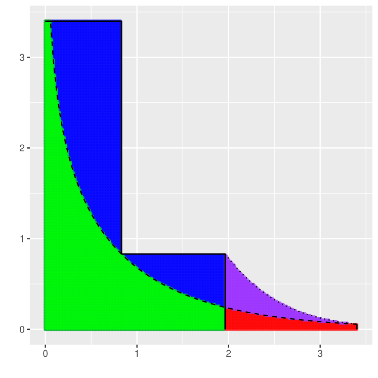
(a) $r=0.4$

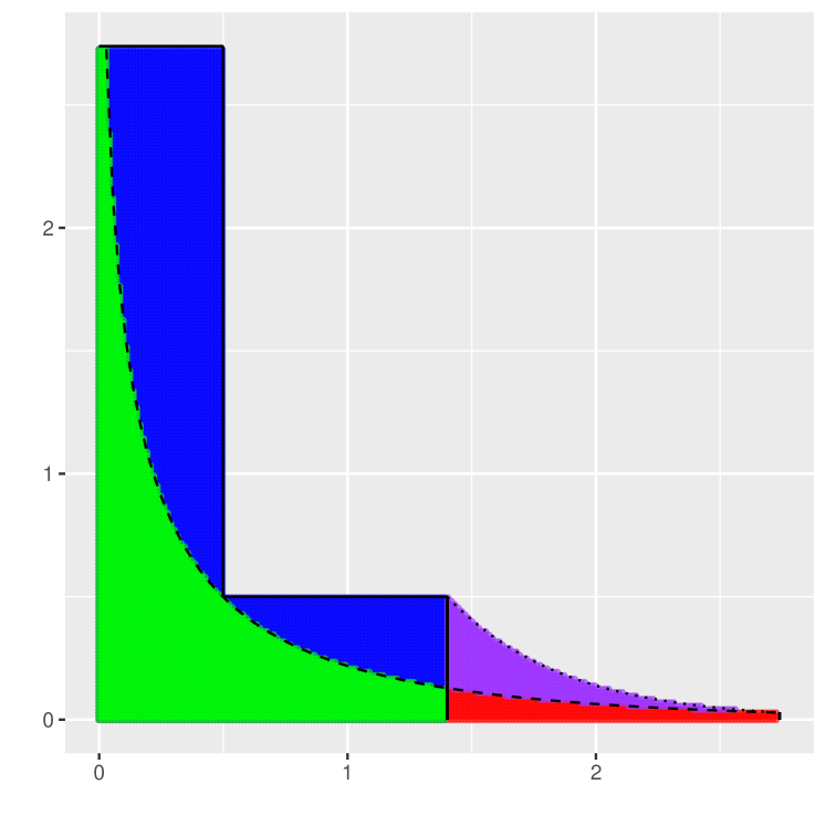
(b) $r=0.2$

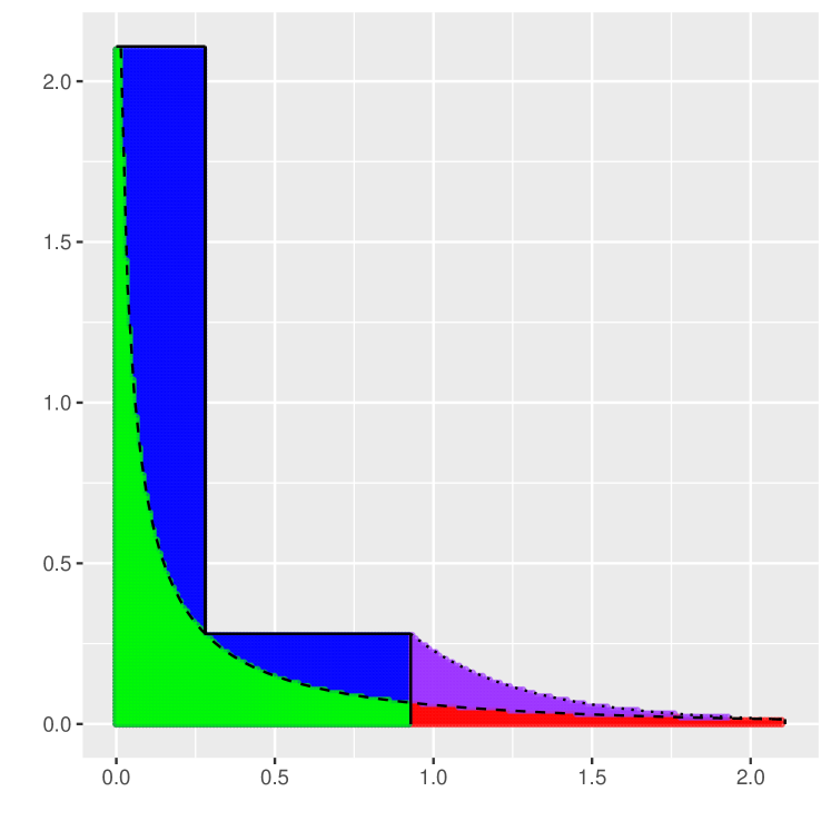
(c) $r=0.1$

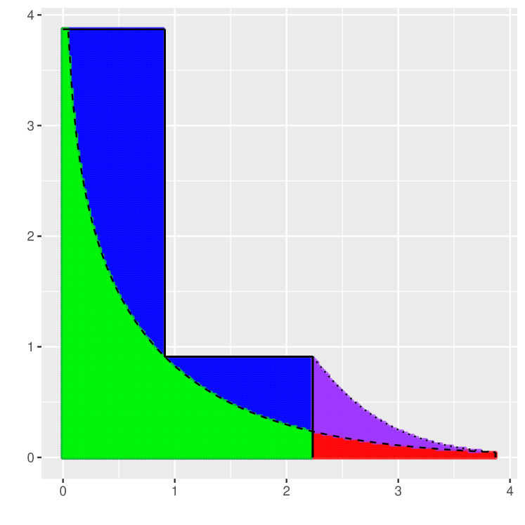
(d) $r=0.4$

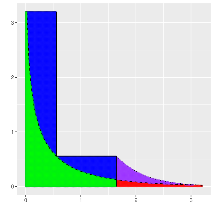
(e) $r=0.2$

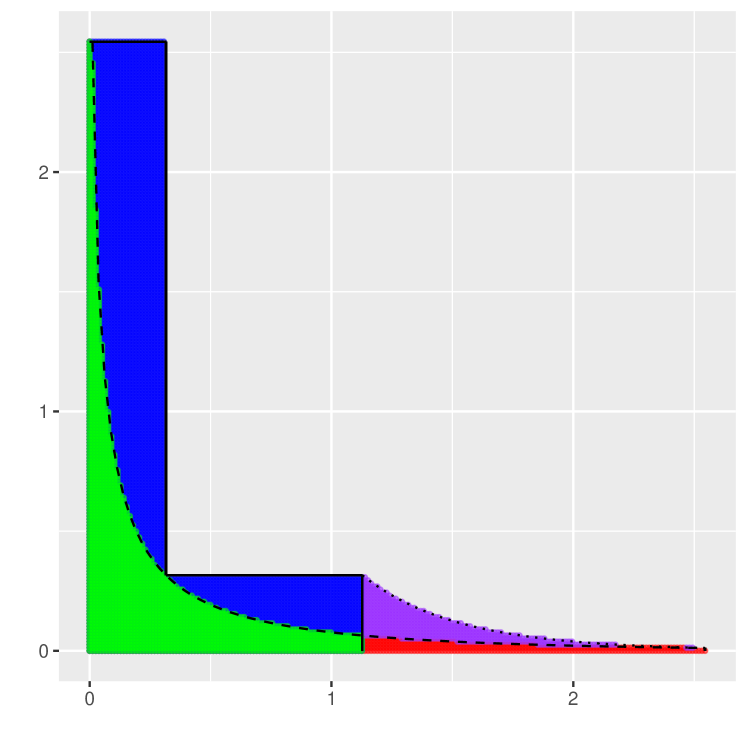
(f) $r=0.1$

Figure 1: Plots of $\log(1+\mathbf{s})=(\log(1+s_{\bm{\alpha}}),\log(1+s_{\bm{\beta}}))$ satisfying sparsity conditions with $N=500$, $d=1000$ for (a)-(c) and $N=1000$, $d=5000$ for (d)-(f) : Green = {$f_{1}(\mathbf{s})\leq r$, $f_{2}(\mathbf{s})\leq r$, and $f_{3}(\mathbf{s})\leq r$}; Red = {$f_{1}(\mathbf{s})\leq r$, $f_{3}(\mathbf{s})\leq r$, and $f_{2}(\mathbf{s})>r$}; Blue = {$f_{2}(\mathbf{s})\leq r$, $f_{3}(\mathbf{s})\leq r$, and $f_{1}(\mathbf{s})>r$}; Purple = {$f_{3}(\mathbf{s})\leq r$, $f_{1}(\mathbf{s})>r$, and $f_{2}(\mathbf{s})>r$}. Lines {$f_{1}(\mathbf{s})=r$}, $\{f_{2}(\mathbf{s})=r\}$, and $\{f_{3}(\mathbf{s})=r\}$ are dashed, solid, and dotted. With $R\equiv 1$ and all models well specified, Chernozhukov et al. (2018) requires $f_{1}(\mathbf{s})=o(1)$ (green + red), Bradic, Wager and Zhu (2019) requires $f_{2}(\mathbf{s})=o(1)$ (green + blue), and the proposed method only requires $f_{3}(\mathbf{s})=o(1)$ (green + red + blue + purple).

Supervised causal

With $R\equiv 1$, our approach outperforms existing methods by relaxing model correctness and sparsity; see Table 4.1. Our proposal is closest to model DR estimators of Smucler, Rotnitzky and Robins (2019), Tan (2020) and Avagyan and Vansteelandt (2021). Our approach introduces an additional parameter tailored to the decaying MAR setting, and we utilize asymmetric cross-fitting, leading to more relaxed sparsity conditions. While previous work required the product of two sparsity levels to be on the order of $n$, our approach allows for this product to be on the order of $n^{3/2}$ or $n^{5/4}$ depending on which model is correctly specified. Although Bradic, Wager and Zhu (2019) shares a similar cross-fitting strategy, their estimator’s implementation is challenging due to non-convex constraints. Furthermore, our proposed estimator exhibits model DR and rate DR with weaker sparsity.

In the following, we clarify the above and consider the following cases: (M1) both nuisance models are correctly specified, (M2) only the OR model is correctly specified, and (M3) only the PS model is correctly specified. Important quantities with $\mathbf{s}=(s_{\bm{\alpha}},s_{\bm{\beta}})$ are

$$f_{1}(\mathbf{s}) :={s_{\bm{\alpha}}\log d/N}\lor{s_{\bm{\beta}}\log d/N}\lor{\sqrt{s_{\bm{\alpha}}s_{\bm{\beta}}}\log d/\sqrt{N}},$$

$$f_{2}(\mathbf{s}) :=\left({s_{\bm{\alpha}}\log d/N^{3/4}}\lor{s_{\bm{\beta}}\log d/\sqrt{N}}\right)\land\left({s_{\bm{\alpha}}\log d/\sqrt{N}}\lor{s_{\bm{\beta}}\log d/N}\right),\;\;\mbox{and}$$

$$f_{3}(\mathbf{s}) :=f_{1}(\mathbf{s})\land f_{2}(\mathbf{s})\land\left\{\left(s_{\bm{\alpha}}\log d/N\right)\lor\left(s_{\bm{\beta}}\log d/\sqrt{N}\right)\lor\left(s_{\bm{\alpha}}^{2/3}s_{\bm{\beta}}^{1/3}\log d/N^{2/3}\right)\right\}.$$

(M1) $m(\cdot)=m^{*}(\cdot)$ and $\gamma_{N}(\cdot)=\gamma_{N}^{*}(\cdot)$. While Chernozhukov et al. (2018) requires $f_{1}(\mathbf{s})=o(1)$ for rate DR, and Bradic, Wager and Zhu (2019) relies on $f_{2}(\mathbf{s})=o(1)$ for sparsity DR, our method allows for a more flexible and general sparsity setting $f_{3}(\mathbf{s})=o(1)$, as illustrated in Figure 1 – our work combines all four colors, where the area colored in purple denotes the sparsity scenario new to the literature.

(M2) $m(\cdot)=m^{*}(\cdot)$ and $\gamma_{N}(\cdot)\neq\gamma_{N}^{*}(\cdot)$. We achieve the coveted model DR property while requiring the same sparsity as in (M1), i.e., $f_{3}(\mathbf{s})=o(1)$. Comparatively, the best result in the existing literature, Smucler, Rotnitzky and Robins (2019), still necessitates a stronger condition of $f_{1}(\mathbf{s})=o(1)$, while Bradic, Wager and Zhu (2019) is valid only for correctly specified models. Further details and comparisons can be found in Table 4.1.

(M3) $m(\cdot)\neq m^{*}(\cdot)$ and $\gamma_{N}(\cdot)=\gamma_{N}^{*}(\cdot)$. Our sparsity conditions are once again weaker. The correctness of OR and PS models affects the required sparsity conditions differently. When the PS model is misspecified, we do not require any additional assumptions compared with (M1). However, when the OR model is misspecified, Smucler, Rotnitzky and Robins (2019) and our proposed method further require an ultra-sparse PS – this is originated from the linear approximation of the non-linear PS model; see $\Delta_{3}$ in Section 4.2. By using the non-cross-fitted PS estimate, we allow a weaker product rate condition $s_{\bm{\alpha}}\sqrt{s_{\bm{\beta}}}=o(N)$ (omitting the logarithm terms) instead of the usual product rate condition $s_{\bm{\alpha}}s_{\bm{\beta}}=o(N)$ – a condition that is always required in Smucler, Rotnitzky and Robins (2019). Although Tan (2020); Ning, Sida and Imai (2020); Avagyan and Vansteelandt (2021); Dukes and Vansteelandt (2021); Dukes, Avagyan and Vansteelandt (2020) also provide robust inference for the ATE when the OR model is misspecified, they require ultra-sparse conditions for both nuisances, whereas we only need the PS model to be ultra-sparse.

5 Simulation studies

We evaluate the general DR-DMAR SS estimator and the bias-reduced DR-DMAR SS estimators using various data-generating processes (DGPs).

5.1 Results under the decaying MAR setting

We consider three types of DGPs in our simulation studies: (a) linear OR models, logistic (product) PS models; (b) linear OR models, non-logistic PS models; and (c) non-linear OR models, logistic PS models. We consider i.i.d. truncated normal covariates $\mathbf{X}_{ij}\sim^{\mathrm{iid}}Z_{\mathrm{trun},2}$ and $\mathbf{X}_{i1}=1$ for each $i\in\{1,\dots,N\}$ and $j\in\{2,\dots,d\}$, where $Z_{\mathrm{trun},2}\sim Z\mid\{|Z|<2\}$ and $Z\sim\mathcal{N}(0,1)$.

(a) Linear OR models, logistic PS models

For $j\in\{0,1\}$ and any $\mathbf{x}\in\mathbb{R}^{d}$, we set

$$\gamma_{N}(j,\mathbf{x})=g(\mathbf{x}^{T}\bm{\beta}(j)),\;\;\pi(\mathbf{x})=\frac{\gamma_{N}(1,\mathbf{x})+1-\gamma_{N}(0,\mathbf{x})}{2},$$ (5.1)

$$p_{N}(1,\mathbf{x})=\frac{\gamma_{N}(1,\mathbf{x})}{\pi(\mathbf{x})},\;\;{\color[rgb]{0,0,0}\mbox{and}}\;\;p_{N}(0,\mathbf{x})=\frac{\gamma_{N}(0,\mathbf{x})}{1-\pi(\mathbf{x})}.$$ (5.2)

We then consider

$$T_{i}\mid\mathbf{X}_{i}\sim\mathrm{Bernoulli}(\pi(\mathbf{X}_{i}))\;\;{\color[rgb]{0,0,0}\mbox{and}}\;\;R_{i}\mid(\mathbf{X}_{i},T_{i}=j)\sim\mathrm{Bernoulli}(p_{N}(j,\mathbf{X}_{i})).$$ (5.3)

Finally, we set linear OR models as follows:

$$Y_{i}(j)=\mathbf{X}_{i}^{T}\bm{\alpha}(j)+\delta_{i},\;\;{\color[rgb]{0,0,0}\mbox{and}}\;\;R_{i}Y_{i}=R_{i}Y_{i}(T_{i}),\;\;\;\mbox{where}\;\;\delta_{i}\sim\mathcal{N}(0,1).$$ (5.4)

(b) Linear OR models, non-logistic PS models

We use $\pi(\mathbf{x})=0.3\sin(\mathbf{x}^{T}\bm{\omega})+0.5$ and $p_{N}(j,\mathbf{x})=g(\mathbf{x}^{T}\bm{\beta}(j))$. The treatment and missingness indicators $(T_{i},R_{i})$ follow (5.3), and the outcomes $Y_{i}(j)$ are determined as in (5.4).

Table 5.1: Simulation results for DGP (a). Bias: empirical bias; RMSE: root mean square error; Length: average length of the $95\%$ confidence intervals; Coverage: average coverage of the $95\%$ confidence intervals; ESD: empirical standard deviation; ASD: average of estimated standard deviations. Bias, RMSE, Length, ESD, and ASD are calculated based on medians.

Estimator	Bias	RMSE	Length	Coverage	ESD	ASD
	DGP (a) $N=10000$, $d=51$, $s_{\bm{\alpha}}=3$, $s_{\bm{\beta}}=3$, $\gamma_{N,j}=0.05~{}(N\gamma_{N,j}=500)$ $\forall j\in\{0,1\}$
$\widehat{\mu}_{\mbox{\tiny oracle}}$	0.007	0.102	0.540	0.948	0.154	0.138
$\widehat{\mu}_{\mbox{\tiny MCAR}}$	0.003	0.090	0.374	0.828	0.136	0.095
$\widehat{\mu}_{\mbox{\tiny SS-Lasso}}$	0.008	0.100	0.470	0.906	0.147	0.120
$\widehat{\mu}_{\mbox{\tiny SS-RF}}$	-0.026	0.151	0.619	0.832	0.214	0.158
$\widehat{\mu}_{\mbox{\tiny BRSS}}$	0.004	0.102	0.503	0.908	0.152	0.128
	DGP (a) $N=10000$, $d=51$, $s_{\bm{\alpha}}=3$, $s_{\bm{\beta}}=3$, $\gamma_{N,j}=0.1~{}(N\gamma_{N,j}=1000)$ $\forall j\in\{0,1\}$
$\widehat{\mu}_{\mbox{\tiny oracle}}$	0.006	0.075	0.428	0.956	0.111	0.109
$\widehat{\mu}_{\mbox{\tiny MCAR}}$	0.003	0.067	0.329	0.902	0.101	0.084
$\widehat{\mu}_{\mbox{\tiny SS-Lasso}}$	0.004	0.073	0.391	0.934	0.107	0.100
$\widehat{\mu}_{\mbox{\tiny SS-RF}}$	-0.023	0.097	0.422	0.848	0.139	0.108
$\widehat{\mu}_{\mbox{\tiny BRSS}}$	0.008	0.073	0.409	0.942	0.111	0.104
	DGP (a) $N=5000$, $d=201$, $s_{\bm{\alpha}}=3$, $s_{\bm{\beta}}=3$, $\gamma_{N,j}=0.1~{}(N\gamma_{N,j}=500)$ $\forall j\in\{0,1\}$
$\widehat{\mu}_{\mbox{\tiny oracle}}$	-0.014	0.098	0.597	0.954	0.145	0.152
$\widehat{\mu}_{\mbox{\tiny MCAR}}$	-0.011	0.091	0.466	0.878	0.136	0.119
$\widehat{\mu}_{\mbox{\tiny SS-Lasso}}$	-0.011	0.095	0.522	0.936	0.144	0.133
$\widehat{\mu}_{\mbox{\tiny BRSS}}$	-0.012	0.099	0.555	0.924	0.145	0.142
	DGP (a) $N=10000$, $d=201$, $s_{\bm{\alpha}}=3$, $s_{\bm{\beta}}=3$, $\gamma_{N,j}=0.1~{}(N\gamma_{N,j}=1000)$ $\forall j\in\{0,1\}$
$\widehat{\mu}_{\mbox{\tiny oracle}}$	-0.013	0.080	0.424	0.964	0.112	0.108
$\widehat{\mu}_{\mbox{\tiny MCAR}}$	-0.010	0.069	0.329	0.900	0.103	0.084
$\widehat{\mu}_{\mbox{\tiny SS-Lasso}}$	-0.012	0.074	0.379	0.946	0.109	0.097
$\widehat{\mu}_{\mbox{\tiny BRSS}}$	-0.014	0.079	0.402	0.958	0.114	0.103

(c) Non-linear OR models, logistic PS models

We consider (5.1)-(5.3) as in part (a) but set quadratic OR models with $\mathbf{X}_{i}^{2}:=(\mathbf{X}_{i1}^{2},\dots,\mathbf{X}_{id}^{2})^{T}$ and

$$Y_{i}(j)=\mathbf{X}_{i}^{T}\bm{\alpha}(j)+(\mathbf{X}_{i}^{2})^{T}\bm{\eta}(j)+\delta_{i},\;\;R_{i}Y_{i}=R_{i}Y_{i}(T_{i}).$$ (5.5)

The parameter values across all the DGPs above are chosen as follows: $\bm{\alpha}(1):=3(1,1,\bm{1}_{s_{\bm{\alpha}}-1}^{T}/\sqrt{s_{\bm{\alpha}}-1},0,\dots,0)^{T}\in\mathbb{R}^{d},\;\;\bm{\alpha}(0):=-\bm{\alpha}(1),$ $\bm{\beta}(1):=(\beta_{N}(1),1,\bm{1}_{s_{\bm{\beta}}-1}^{T}/(s_{\bm{\beta}}-1),0,\dots,0)^{T}\in\mathbb{R}^{d},$ $\bm{\beta}(0):=(\beta_{N}(0),-1,-\bm{1}_{s_{\bm{\beta}}-1}^{T}/(s_{\bm{\beta}}-1),0,\dots,0)^{T}\in\mathbb{R}^{d},$ $\bm{\omega}:=(0,1,$ $\bm{1}_{s_{\bm{\beta}}-1}^{T}/(s_{\bm{\beta}}-1),0,\dots,0)^{T}\in\mathbb{R}^{d},$ $\bm{\eta}(1):=(0,1,\bm{1}_{s_{\bm{\alpha}}-1}^{T}/\sqrt{s_{\bm{\alpha}}-1},0,\dots,0)^{T}\in\mathbb{R}^{d},\;\;\bm{\eta}(0):=-\bm{\eta}(1)\color[rgb]{0,0,0}{,}$ where for any positive integer $s\geq 1$, $\bm{1}_{s}:=\{1,\dots,1\}\in\mathbb{R}^{s}$ and $\bm{1}_{0}:=\emptyset$, and $\beta_{N}(1),\beta_{N}(0)$ are chosen such that $\mathbb{E}(RT)=\gamma_{N,1}$ and $\mathbb{E}\{R(1-T)\}=\gamma_{N,0}$.

We consider: (1) Oracle estimator $\widehat{\mu}_{\text{oracle}}$: DR-DMAR SS estimator with true values as nuisances. (2) $\widehat{\mu}_{\text{MCAR}}$: SS estimator treating missingness as MCAR (the selection bias is ignored), estimated using Lasso for OR and PS. (3) $\widehat{\mu}_{\text{SS-Lasso}}$: DR-DMAR SS estimator with Lasso for OR and PS. (4) $\widehat{\mu}_{\text{SS-RF}}$: DR-DMAR SS estimator with random forest estimates (up to $d=51$ dimensions). (5) The bias-reduced $\widehat{\mu}_{\mbox{\tiny BRSS}}$ of (4.6). The tuning parameters are chosen using 5-fold cross-validation and results, repeated $500$ times, are presented in Tables 5.1-5.3.

Table 5.2: Simulation results for DGP (b). The rest of the caption details remain the same as those in Table 5.1.

Estimator	Bias	RMSE	Length	Coverage	ESD	ASD
	DGP (b) $N=10000$, $d=51$, $s_{\bm{\alpha}}=2$, $s_{\bm{\beta}}=6$, $\gamma_{N,j}=0.05~{}(N\gamma_{N,j}=500)$ $\forall j\in\{0,1\}$
$\widehat{\mu}_{\mbox{\tiny oracle}}$	-0.012	0.084	0.565	0.964	0.125	0.144
$\widehat{\mu}_{\mbox{\tiny MCAR}}$	-0.005	0.067	0.286	0.812	0.099	0.073
$\widehat{\mu}_{\mbox{\tiny SS-Lasso}}$	-0.004	0.079	0.390	0.912	0.118	0.099
$\widehat{\mu}_{\mbox{\tiny SS-RF}}$	-0.023	0.101	0.403	0.824	0.147	0.103
$\widehat{\mu}_{\mbox{\tiny BRSS}}$	0.001	0.075	0.470	0.946	0.111	0.120
	DGP (b) $N=10000$, $d=51$, $s_{\bm{\alpha}}=2$, $s_{\bm{\beta}}=6$, $\gamma_{N,j}=0.1~{}(N\gamma_{N,j}=1000)$ $\forall j\in\{0,1\}$
$\widehat{\mu}_{\mbox{\tiny oracle}}$	-0.007	0.075	0.412	0.954	0.110	0.105
$\widehat{\mu}_{\mbox{\tiny MCAR}}$	-0.001	0.061	0.250	0.856	0.090	0.064
$\widehat{\mu}_{\mbox{\tiny SS-Lasso}}$	-0.005	0.065	0.312	0.916	0.096	0.080
$\widehat{\mu}_{\mbox{\tiny SS-RF}}$	-0.015	0.070	0.297	0.852	0.097	0.076
$\widehat{\mu}_{\mbox{\tiny BRSS}}$	-0.005	0.068	0.366	0.942	0.100	0.093
	DGP (b) $N=5000$, $d=201$, $s_{\bm{\alpha}}=2$, $s_{\bm{\beta}}=6$, $\gamma_{N,j}=0.1~{}(N\gamma_{N,j}=500)$ $\forall j\in\{0,1\}$
$\widehat{\mu}_{\mbox{\tiny oracle}}$	-0.008	0.106	0.572	0.936	0.156	0.146
$\widehat{\mu}_{\mbox{\tiny MCAR}}$	-0.008	0.078	0.354	0.872	0.118	0.090
$\widehat{\mu}_{\mbox{\tiny SS-Lasso}}$	-0.006	0.089	0.418	0.884	0.135	0.107
$\widehat{\mu}_{\mbox{\tiny BRSS}}$	-0.010	0.089	0.480	0.918	0.129	0.122
	DGP (b) $N=10000$, $d=201$, $s_{\bm{\alpha}}=2$, $s_{\bm{\beta}}=6$, $\gamma_{N,j}=0.1~{}(N\gamma_{N,j}=1000)$ $\forall j\in\{0,1\}$
$\widehat{\mu}_{\mbox{\tiny oracle}}$	0.001	0.078	0.412	0.952	0.115	0.105
$\widehat{\mu}_{\mbox{\tiny MCAR}}$	-0.004	0.062	0.270	0.880	0.094	0.069
$\widehat{\mu}_{\mbox{\tiny SS-Lasso}}$	-0.001	0.066	0.300	0.920	0.099	0.077
$\widehat{\mu}_{\mbox{\tiny BRSS}}$	0.001	0.074	0.357	0.952	0.110	0.091

Among the four estimators, $\widehat{\mu}_{\mbox{\tiny SS-RF}}$ exhibits larger bias and RMSE due to slower convergence rates, while the remaining estimators demonstrate smaller biases compared to RMSE in Tables 5.1 and 5.2. In contrast, in Table 5.3, notable biases and larger RMSEs are observed for $\widehat{\mu}_{\mbox{\tiny SS-RF}}$, $\widehat{\mu}_{\mbox{\tiny SS-Lasso}}$, and $\widehat{\mu}_{\mbox{\tiny MCAR}}$, while $\widehat{\mu}_{\mbox{\tiny BRSS}}$ outperforms them significantly. The poor performance of $\widehat{\mu}_{\mbox{\tiny MCAR}}$ in all DGPs is attributed to its incorrect treatment of the labeling indicator’s PS as a constant, resulting in significant undercoverage, particularly in Table 5.3. On the other hand, $\widehat{\mu}_{\mbox{\tiny SS-Lasso}}$ provides valid inference with correct nuisance model specification (as per Theorem A.2), but its reliability diminishes when model misspecification occurs, leading to underestimation of variance and large bias in Tables 5.2 and 5.3. In contrast, the $\widehat{\mu}_{\mbox{\tiny SS-RF}}$ estimator, relying on non-parametric nuisance estimators, fails to satisfy the ‘product-rate’ condition, resulting in undercoverage in all DGPs. The coverage results in Tables 5.1-5.3 support the inference quality of $\widehat{\mu}_{\mbox{\tiny BRSS}}$ when one nuisance is misspecified, as per Corollary 4.6. Notably, Table 5.2 exhibits excellent coverage with minor deviations for smaller effective sample size and higher dimension, while in Table 5.3, $\widehat{\mu}_{\mbox{\tiny BRSS}}$ consistently delivers strong performance for higher sample sizes where $\widehat{\mu}_{\mbox{\tiny MCAR}}$, $\widehat{\mu}_{\mbox{\tiny SS-Lasso}}$, and $\widehat{\mu}_{\mbox{\tiny SS-RF}}$ fail, respectively.

Table 5.3: Simulation results for DGP (c). The rest of the caption details remain the same as those in Table 5.1.

Estimator	Bias	RMSE	Length	Coverage	ESD	ASD
	DGP (c) $N=10000$, $d=51$, $s_{\bm{\alpha}}=6$, $s_{\bm{\beta}}=2$, $\gamma_{N,j}=0.05~{}(N\gamma_{N,j}=500)$ $\forall j\in\{0,1\}$
$\widehat{\mu}_{\mbox{\tiny oracle}}$	-0.013	0.077	0.463	0.948	0.110	0.118
$\widehat{\mu}_{\mbox{\tiny MCAR}}$	-0.722	0.722	0.484	0.002	0.168	0.124
$\widehat{\mu}_{\mbox{\tiny SS-Lasso}}$	-0.255	0.263	0.752	0.712	0.193	0.192
$\widehat{\mu}_{\mbox{\tiny SS-RF}}$	-0.282	0.288	0.749	0.668	0.221	0.191
$\widehat{\mu}_{\mbox{\tiny BRSS}}$	-0.116	0.139	0.637	0.884	0.153	0.163
	DGP (c) $N=10000$, $d=51$, $s_{\bm{\alpha}}=6$, $s_{\bm{\beta}}=2$, $\gamma_{N,j}=0.1~{}(N\gamma_{N,j}=1000)$ $\forall j\in\{0,1\}$
$\widehat{\mu}_{\mbox{\tiny oracle}}$	-0.010	0.063	0.390	0.954	0.092	0.099
$\widehat{\mu}_{\mbox{\tiny MCAR}}$	-0.642	0.642	0.394	0.000	0.132	0.101
$\widehat{\mu}_{\mbox{\tiny SS-Lasso}}$	-0.181	0.182	0.576	0.740	0.151	0.147
$\widehat{\mu}_{\mbox{\tiny SS-RF}}$	-0.186	0.188	0.525	0.674	0.164	0.134
$\widehat{\mu}_{\mbox{\tiny BRSS}}$	-0.044	0.095	0.493	0.930	0.133	0.126
	DGP (c) $N=5000$, $d=201$, $s_{\bm{\alpha}}=6$, $s_{\bm{\beta}}=2$, $\gamma_{N,j}=0.1~{}(N\gamma_{N,j}=500)$ $\forall j\in\{0,1\}$
$\widehat{\mu}_{\mbox{\tiny oracle}}$	-0.009	0.096	0.550	0.956	0.143	0.140
$\widehat{\mu}_{\mbox{\tiny MCAR}}$	-0.652	0.652	0.566	0.026	0.186	0.144
$\widehat{\mu}_{\mbox{\tiny SS-Lasso}}$	-0.292	0.292	0.745	0.648	0.199	0.190
$\widehat{\mu}_{\mbox{\tiny BRSS}}$	-0.134	0.160	0.685	0.862	0.179	0.175
	DGP (c) $N=10000$, $d=201$, $s_{\bm{\alpha}}=6$, $s_{\bm{\beta}}=2$, $\gamma_{N,j}=0.1~{}(N\gamma_{N,j}=1000)$ $\forall j\in\{0,1\}$
$\widehat{\mu}_{\mbox{\tiny oracle}}$	-0.009	0.064	0.391	0.964	0.090	0.100
$\widehat{\mu}_{\mbox{\tiny MCAR}}$	-0.637	0.637	0.395	0.000	0.128	0.101
$\widehat{\mu}_{\mbox{\tiny SS-Lasso}}$	-0.223	0.223	0.556	0.660	0.134	0.142
$\widehat{\mu}_{\mbox{\tiny BRSS}}$	-0.065	0.091	0.488	0.894	0.117	0.125
	DGP (c) $N=20000$, $d=201$, $s_{\bm{\alpha}}=6$, $s_{\bm{\beta}}=2$, $\gamma_{N,j}=0.1~{}(N\gamma_{N,j}=2000)$ $\forall j\in\{0,1\}$
$\widehat{\mu}_{\mbox{\tiny oracle}}$	-0.010	0.050	0.276	0.948	0.071	0.070
$\widehat{\mu}_{\mbox{\tiny MCAR}}$	-0.628	0.628	0.278	0.000	0.089	0.071
$\widehat{\mu}_{\mbox{\tiny SS-Lasso}}$	-0.168	0.168	0.407	0.622	0.103	0.104
$\widehat{\mu}_{\mbox{\tiny BRSS}}$	-0.033	0.063	0.349	0.930	0.090	0.089

5.2 A degenerate setting with outcomes fully observed

In the setting of fully observed outcomes ($R_{i}=1$ for all $i\in{1,\dots,N}$), we examine the cases where one of the nuisance models is misspecified and highlight what is different from Section 5.1.

(d) Linear OR models, non-logistic PS model

$$\pi(\mathbf{x})=\exp(\mathbf{x}^{T}\bm{\beta}_{d})/\{1+\exp(\mathbf{x}^{T}\bm{\beta}_{d})\}\{0.3\sin(\mathbf{x}^{T}\bm{\beta}_{d})+0.7\}\;\;\mbox{and}\;\;Y_{i}(j)=\mathbf{X}_{i}^{T}\bm{\alpha}_{d}(j)+\delta_{i}.$$

(e) Non-linear OR models, logistic PS model

$$\pi(\mathbf{x})=\exp(\mathbf{x}^{T}\bm{\beta}_{e})/\{1+\exp(\mathbf{x}^{T}\bm{\beta}_{e})\}\;\;\mbox{and}\;\;Y_{i}(j)=\mathbf{X}_{i}^{T}\bm{\alpha}_{e}(j)+(\mathbf{X}_{i}^{2})^{T}\bm{\eta}_{e}(j)+\delta_{i}.$$

The parameters for DGPs (d) and (e) are $\bm{\alpha}_{d}(1):=3(1,0.9^{1},\dots,0.9^{d-1})^{T}\in\mathbb{R}^{d},\;\;\bm{\alpha}_{d}(0)=-\bm{\alpha}_{d}(1),\;\;\bm{\alpha}_{e}(j)=\bm{\alpha}_{d}(j),$ $\bm{\eta}_{e}(1):=(0,0.9^{1},\dots,0.9^{d-1})^{T}\in\mathbb{R}^{d},\;\;\bm{\eta}_{e}(0)=-\bm{\eta}_{e}(1),$ $\bm{\beta}_{d}:=(0.99,0.5\cdot 0.7^{1},\dots,0.5\cdot 0.7^{d-1})^{T}\in\mathbb{R}^{d},\;\;\bm{\beta}_{e}:=(0.2247,0.7^{1},\dots,0.7^{d-1})^{T}\in\mathbb{R}^{d}.$ Here, we compare the numerical performance of our proposed bias-reduced estimator $\widehat{\mu}_{\mbox{\tiny BRSS}}$ with $\widehat{\mu}_{\mbox{\tiny Smucler}}$ by Smucler, Rotnitzky and Robins (2019); as per Table 4.1 their estimator is the most competitive in the existing literature. The nuisance parameters in DGPs (d) and (e) exhibit a ‘weakly sparse’ nature, with bounded $\ell_{1}$-norms but $\ell_{0}$-norms equal to the dimension. In Table 5.4, it is observed that the estimator $\widehat{\mu}_{\mbox{\tiny Smucler}}$ suffers from substantial biases. Consequently, the coverages based on $\widehat{\mu}_{\mbox{\tiny Smucler}}$ are relatively poor. In contrast, our proposed estimator $\widehat{\mu}_{\mbox{\tiny BRSS}}$ exhibits significantly smaller biases, leading to improved coverages. Additionally, $\widehat{\mu}_{\mbox{\tiny BRSS}}$ achieves smaller RMSEs compared to $\widehat{\mu}_{\mbox{\tiny Smucler}}$ for both DGPs (d) and (e).

Table 5.4: Simulation results for DGPs (d) and (e). The rest of the caption details remain the same as those in Table 5.1.

Estimator	Bias	RMSE	Length	Coverage	ESD	ASD
	DGP (d) $N=300$, $d=51$, $s_{\bm{\alpha}}=51$, $s_{\bm{\beta}}=51$
$\widehat{\mu}_{\mbox{\tiny oracle}}$	0.002	0.411	2.518	0.948	0.608	0.642
$\widehat{\mu}_{\mbox{\tiny Smucler}}$	-0.560	0.637	2.626	0.870	0.645	0.670
$\widehat{\mu}_{\mbox{\tiny BRSS}}$	-0.208	0.460	2.471	0.928	0.662	0.630
	DGP (e) $N=400$, $d=51$, $s_{\bm{\alpha}}=51$, $s_{\bm{\beta}}=51$
$\widehat{\mu}_{\mbox{\tiny oracle}}$	-0.012	0.375	2.305	0.958	0.564	0.588
$\widehat{\mu}_{\mbox{\tiny Smucler}}$	0.484	0.584	2.479	0.896	0.628	0.632
$\widehat{\mu}_{\mbox{\tiny BRSS}}$	0.104	0.471	2.315	0.942	0.655	0.591

5.3 Results based on the semi-parametric approach

In this section, we further examine the behavior of the semi-parametric bias-reduced DR-DMAR SS estimator, $\widehat{\mu}_{\tiny\mbox{SP-BRSS}}$, proposed in Section 4.3. The following case is considered.

(f) Non-linear OR models, non-logistic treatment PS model, logistic labeling PS model

Generate $\pi(\mathbf{x})=0.3\cos(\mathbf{x}^{T}\bm{\beta})+0.5$, $p_{N}(j,\mathbf{x})=\exp\{\mathbf{x}^{T}\bm{\beta}^{\prime}(j)\}/[1+\exp\{\mathbf{x}^{T}\bm{\beta}^{\prime}(j)\}]$, and (5.5). Choose $\bm{\alpha}(j)$ and $\bm{\eta}(j)$ as in Section 5.1 with $s_{\bm{\alpha}}=5$, $\bm{\beta}:=2(0,0.9^{1},\dots,0.9^{d-1})^{T}$, $\bm{\beta}^{\prime}(1):=(\bm{\beta}_{N}^{\prime}(1),1,\bm{1}_{4}^{T}/4,0,\dots,0)^{T}\in\mathbb{R}^{d}$, and $\bm{\beta}^{\prime}(0):=(\bm{\beta}_{N}^{\prime}(0),-1,-\bm{1}_{4}^{T}/4,0,\dots,0)^{T}\in\mathbb{R}^{d}$, where $\bm{\beta}_{N}^{\prime}(1)$ and $\bm{\beta}_{N}^{\prime}(0)$ are chosen such that $\mathbb{E}(RT)=\gamma_{N,1}$ and $\mathbb{E}\{R(1-T)\}=\gamma_{N,0}$.

We compare the numerical performance of the estimators considered in Section 5.1 with $\widehat{\mu}_{\tiny\mbox{SP-BRSS}}$, where the treatment PS function $\pi(\cdot)$ is estimated using random forests. As shown in Table 5.5, $\widehat{\mu}_{\tiny\mbox{MCAR}}$ provides large biases and very poor coverages since the true labeling mechanism is not MCAR. The performance of $\widehat{\mu}_{\tiny\mbox{SS-Lasso}}$ is also relatively poor since both nuisance models are misspecified – the OR models are non-linear and the product PS models are non-logistic. The parametric BRSS estimator $\widehat{\mu}_{\tiny\mbox{BRSS}}$ provides slightly smaller biases and RMSEs, although the working models are still misspecified. The fully non-parametric estimator $\widehat{\mu}_{\tiny\mbox{SS-RF}}$ performs similarly as, better than, and worse than $\widehat{\mu}_{\tiny\mbox{BRSS}}$ when $(d,\gamma_{N,j})$ are chosen as $(31,0.05)$, $(51,0.05)$, and $(51,0.1)$, respectively. Although the non-parametric nuisance estimates are consistent, the convergence rates are relatively slow as the ‘effective sample size’ for the OR and product PS estimation is only $500$ when $\gamma_{N,j}=0.05$ and $1000$ when $\gamma_{N,j}=0.1$ (with a moderate dimension $d=31$ or $d=51$), resulting in relatively large biases for the final ATE estimation. Lastly, by making full use of the large sized $(T_{i},\mathbf{X}_{i})$ and estimate $\pi(\cdot)$ non-parametrically while keeping other working models parametrically, the proposed semi-parametric BRSS estimator $\widehat{\mu}_{\tiny\mbox{SP-BRSS}}$ outperforms all the ATE estimators above, although the OR models are misspecified.

Table 5.5: Simulation results for DGP (f). The rest of the caption details remain the same as those in Table 5.1.

Estimator	Bias	RMSE	Length	Coverage	ESD	ASD
	DGP (f) $N=10000$, $d=31$, $\gamma_{N,j}=0.05~{}(N\gamma_{N,j}=500)$ $\forall j\in\{0,1\}$
$\widehat{\mu}_{\mbox{\tiny oracle}}$	-0.007	0.083	0.500	0.954	0.122	0.127
$\widehat{\mu}_{\mbox{\tiny MCAR}}$	-0.724	0.724	0.493	0.004	0.186	0.126
$\widehat{\mu}_{\mbox{\tiny SS-Lasso}}$	-0.224	0.233	0.774	0.736	0.217	0.198
$\widehat{\mu}_{\mbox{\tiny SS-RF}}$	-0.172	0.198	0.736	0.774	0.246	0.188
$\widehat{\mu}_{\mbox{\tiny BRSS}}$	-0.170	0.180	0.640	0.800	0.182	0.163
$\widehat{\mu}_{\mbox{\tiny SP-BRSS}}$	-0.127	0.158	1.144	0.988	0.195	0.292
	DGP (f) $N=10000$, $d=51$, $\gamma_{N,j}=0.05~{}(N\gamma_{N,j}=500)$ $\forall j\in\{0,1\}$
$\widehat{\mu}_{\mbox{\tiny oracle}}$	-0.011	0.085	0.499	0.942	0.126	0.127
$\widehat{\mu}_{\mbox{\tiny MCAR}}$	-0.727	0.727	0.495	0.006	0.170	0.126
$\widehat{\mu}_{\mbox{\tiny SS-Lasso}}$	-0.284	0.290	0.746	0.664	0.213	0.190
$\widehat{\mu}_{\mbox{\tiny SS-RF}}$	-0.165	0.206	0.732	0.828	0.216	0.187
$\widehat{\mu}_{\mbox{\tiny BRSS}}$	-0.190	0.200	0.634	0.780	0.184	0.162
$\widehat{\mu}_{\mbox{\tiny SP-BRSS}}$	-0.139	0.179	1.136	0.988	0.197	0.290
	DGP (f) $N=10000$, $d=51$, $\gamma_{N,j}=0.1~{}(N\gamma_{N,j}=1000)$ $\forall j\in\{0,1\}$
$\widehat{\mu}_{\mbox{\tiny oracle}}$	-0.018	0.074	0.405	0.944	0.104	0.103
$\widehat{\mu}_{\mbox{\tiny MCAR}}$	-0.614	0.614	0.402	0.002	0.137	0.103
$\widehat{\mu}_{\mbox{\tiny SS-Lasso}}$	-0.255	0.255	0.521	0.534	0.141	0.133
$\widehat{\mu}_{\mbox{\tiny SS-RF}}$	-0.151	0.161	0.498	0.732	0.154	0.127
$\widehat{\mu}_{\mbox{\tiny BRSS}}$	-0.135	0.143	0.478	0.760	0.140	0.122
$\widehat{\mu}_{\mbox{\tiny SP-BRSS}}$	-0.084	0.109	0.799	0.992	0.142	0.204

6 Applications to a pseudo-random dataset

We compare the performance of the proposed estimators using a synthetic dataset obtained from the Atlantic Causal Inference Conference (ACIC) 2019 Data Challenge. We focus on 14 scenarios from the ACIC 2019 dataset, as two scenarios share the same covariate matrix. To examine the performance under model misspecification, we construct $T_{i}$ and $R_{i}$ as in (5.1)-(5.3) and generate the outcome variable $Y_{i}$ as in (5.5) – that is, we consider a correctly specified (logistic) PS model and a misspecified (quadratic) OR model. We set $\bm{\alpha}(1):=(2,2,1,1,1,1,0,\dots,0)^{T}\in\mathbb{R}^{d},\;\;\bm{\alpha}(0):=-\bm{\alpha}(1),$ $\bm{\beta}(1):=(-1.5,0.5,0,\dots,0)^{T}\in\mathbb{R}^{d},\;\;\bm{\beta}(0):=(-1.5,-0.5,0,\dots,0)^{T}\in\mathbb{R}^{d},$ and $\bm{\eta}(1):=0.35(0,2,1,1,1,1,0,\dots,0)^{T}\in\mathbb{R}^{d},\;\;\bm{\eta}(0):=-\bm{\eta}(1).$ We generate 100 sets for each scenario resulting in $14*100=1400$ pseudo-random datasets in total. The covariate matrices have dimensions of $(N,d)=(1000,201)$ in Scenarios 1, 2, 3, 6, 8, and 14, and $(N,d)=(2000,201)$ in the other scenarios. We consider $\widehat{\mu}_{\mbox{\tiny MCAR}}$, $\widehat{\mu}_{\mbox{\tiny SS-Lasso}}$, and $\widehat{\mu}_{\mbox{\tiny BRSS}}$. The results are reported in Table 6.1.

Table 6.1: Results for the pseudo-random dataset. Bias: empirical bias; RMSE: root mean square error; Length: average length of the $95\%$ confidence intervals; Coverage: average coverage of the $95\%$ confidence intervals.

Estimator	Bias	RMSE	Length	Coverage		Bias	RMSE	Length	Coverage
	Scenario 1 $N=1000$, $d=201$					Scenario 2 $N=1000$, $d=201$
$\widehat{\mu}_{\mbox{\tiny MCAR}}$	-0.341	0.403	1.209	0.880		-0.231	0.307	0.994	0.900
$\widehat{\mu}_{\mbox{\tiny SS-Lasso}}$	-0.257	0.398	1.248	0.900		-0.157	0.260	1.057	0.960
$\widehat{\mu}_{\mbox{\tiny BRSS}}$	-0.263	0.322	1.142	0.940		-0.164	0.244	1.004	0.940
	Scenario 3 $N=1000$, $d=201$					Scenario 4 $N=2000$, $d=201$
$\widehat{\mu}_{\mbox{\tiny MCAR}}$	-0.080	0.400	1.879	0.960		-0.237	0.273	0.652	0.760
$\widehat{\mu}_{\mbox{\tiny SS-Lasso}}$	-0.102	0.408	1.958	0.920		-0.144	0.200	0.696	0.930
$\widehat{\mu}_{\mbox{\tiny BRSS}}$	-0.114	0.411	1.906	0.930		-0.095	0.161	0.672	0.960
	Scenario 5 $N=2000$, $d=201$					Scenario 6 $N=1000$, $d=201$
$\widehat{\mu}_{\mbox{\tiny MCAR}}$	-0.290	0.316	0.665	0.650		-0.247	0.313	0.997	0.860
$\widehat{\mu}_{\mbox{\tiny SS-Lasso}}$	-0.187	0.231	0.717	0.870		-0.168	0.266	1.058	0.920
$\widehat{\mu}_{\mbox{\tiny BRSS}}$	-0.118	0.167	0.686	0.980		-0.171	0.245	1.006	0.950
	Scenario 7 $N=2000$, $d=201$					Scenario 8 $N=1000$, $d=201$
$\widehat{\mu}_{\mbox{\tiny MCAR}}$	-0.254	0.290	0.656	0.670		-0.272	0.337	0.956	0.810
$\widehat{\mu}_{\mbox{\tiny SS-Lasso}}$	-0.152	0.217	0.709	0.880		-0.180	0.285	1.019	0.910
$\widehat{\mu}_{\mbox{\tiny BRSS}}$	-0.095	0.158	0.679	0.980		-0.186	0.270	0.975	0.940
	Scenario 9 $N=2000$, $d=201$					Scenario 12 $N=2000$, $d=201$
$\widehat{\mu}_{\mbox{\tiny MCAR}}$	-0.247	0.289	0.666	0.710		-0.250	0.283	0.662	0.710
$\widehat{\mu}_{\mbox{\tiny SS-Lasso}}$	-0.140	0.209	0.718	0.900		-0.147	0.198	0.711	0.890
$\widehat{\mu}_{\mbox{\tiny BRSS}}$	-0.082	0.156	0.687	0.960		-0.093	0.159	0.678	0.990
	Scenario 13 $N=2000$, $d=201$					Scenario 14 $N=1000$, $d=201$
$\widehat{\mu}_{\mbox{\tiny MCAR}}$	-0.236	0.275	0.665	0.720		-0.211	0.297	0.956	0.910
$\widehat{\mu}_{\mbox{\tiny SS-Lasso}}$	-0.132	0.199	0.714	0.860		-0.122	0.259	1.020	0.950
$\widehat{\mu}_{\mbox{\tiny BRSS}}$	-0.084	0.155	0.682	0.990		-0.134	0.242	0.970	0.960
	Scenario 15 $N=2000$, $d=201$					Scenario 16 $N=2000$, $d=201$
$\widehat{\mu}_{\mbox{\tiny MCAR}}$	-0.245	0.278	0.661	0.730		-0.356	0.388	0.832	0.590
$\widehat{\mu}_{\mbox{\tiny SS-Lasso}}$	-0.148	0.202	0.708	0.900		-0.228	0.321	0.911	0.820
$\widehat{\mu}_{\mbox{\tiny BRSS}}$	-0.087	0.149	0.679	0.990		-0.159	0.204	0.812	0.980

Except for Scenario 3, the MCAR estimator exhibits poor performance with large biases and inadequate coverage. In Scenarios 2, 3, 4, 6, 8, and 14, both the SS-Lasso and BRSS estimators perform well, showing similar biases, RMSEs, and coverages close to 95%. However, in Scenarios 5, 7, 9, 12, 13, 15, and 16, BRSS outperforms SS-Lasso with smaller biases, RMSEs, and improved coverages. Additionally, in Scenario 1, BRSS achieves a smaller RMSE and a coverage closer to 95%, while its bias remains comparable to SS-Lasso. Overall, the MCAR estimator’s poor performance is attributed to the mischaracterization of the labeling PS function, while the BRSS estimator exhibits greater stability compared to SS-Lasso due to the misspecified OR model.

7 Discussion

This paper addresses the estimation of the average treatment effect (ATE) in settings where selection bias may occur. We introduce a novel framework called the ‘decaying MAR setting,’ which encompasses both regular selection bias and missing outcome scenarios, providing a more general approach. Within this framework, we propose flexible ATE estimators based on flexible nuisance model estimators, including non-parametric ones. To tackle the challenges of model misspecification, we propose bias-reduced ATE estimators that incorporate carefully designed nuisance estimates and an asymmetric cross-fitting strategy. Our results highlight the crucial role of these design choices in ensuring robust estimation and inference of the ATE, particularly in high-dimensional settings.

In addition to the ATE estimation problem, our framework opens up possibilities for studying estimation and inference of other parameters of interest in the decaying MAR setting. One such parameter is the decaying PS function, which serves as a vital intermediate step for ATE estimation. Further research is needed to explore the validity of non-parametric PS estimators in the decaying PS setup. Additionally, alternative methods like inverse probability weighting and residual balancing can be employed in degenerate supervised settings, but their validity and theoretical properties in this context require further investigation for future research.

Supplementary Material

Supplement to ‘The Decaying Missing-at-Random Framework: Doubly Robust Causal Inference with Partially Labeled Data’. In the Supplement, we provide additional theoretical results, discussions, and proofs related to our main findings. In Section A, we present theoretical results for the estimation of the counterfactual mean and the ATE. Further discussions on estimating PS when the treatment variable $T$ is missing are included in Section B. The proofs of all the main results can be found in Sections C-G.

SUPPLEMENT TO ‘THE DECAYING MISSING-AT-RANDOM FRAMEWORK: DOUBLY ROBUST CAUSAL INFERENCE WITH PARTIALLY LABELED DATA’

This supplementary document contains further discussions, additional theoretical results, and proofs of the main results that could not be accommodated in the main paper. All results and notations are numbered and used as in the main text unless stated otherwise. We summarize the key notations used throughout the main paper and the supplement in Table S.1.

Table S.1: Table of notations (we let $j\in\{0,1\}$ and $k\in\{1,2\}$ in the following table)

Notation	Description
$\mathbf{X}_{i},\mathbf{X}$	The vector of covariates
$T_{i},T$	The treatment indicators
$R_{i},R$	The labeling indicators
$\Gamma_{i}^{(j)},\Gamma^{(j)},\Gamma_{i}:=\Gamma^{(1)}_{i},\Gamma:=\Gamma^{(1)}$	The product indicators
$Y_{i},Y$	The observed outcome of interest
$Y_{i}(j),Y(j)$	The potential outcomes
$N$	The total sample size
$n$	The labeled sample size $n=\sum_{i=1}^{N}R_{i}$
$d$	The dimension of the covariates
$\mathbb{K}$	Number of folds
$M=N/\mathbb{K}$	Number of samples in each fold
$p_{N},p_{N,1}$	The labeling probabilities $\mathbb{P}(R=1)$ and $\mathbb{P}(R=1\mid T=1)$
$\gamma_{N}$	The product probability $\mathbb{P}(\Gamma=1)$
$a_{N,j}$	The inverses of the inverse product PS functions’ expectations
$a_{N}$	The smaller rate among $a_{N,1}$ and $a_{N,0}$
$Na_{N}$	The ‘effective sample size’
$\theta_{j}$	The counterfactual means $\theta_{j}:=\mathbb{E}\{Y(j)\}$
$\mu_{0}$	The ATE parameter $\mu_{0}:=\theta_{1}-\theta_{0}$
$m(j,\cdot),m(\cdot):=m(1,\cdot)$	The true OR functions
$\pi(\cdot),\pi(j,\cdot)$	The true treatment PS functions
$p_{N}(\cdot),p_{N}(j,\cdot),p_{N,1}(\cdot)=p_{N}(1,\cdot)$	The true labeling PS functions
$\gamma_{N}(j,\cdot),\gamma_{N}(\cdot)=\gamma_{N}(1,\cdot)$	The true product PS functions
$\widehat{m}(j,\cdot),\widehat{m}(\cdot):=\widehat{m}(1,\cdot),$	The OR estimators
$\widehat{\gamma}_{N}(j,\cdot),\widehat{\gamma}_{N}(\cdot):=\widehat{\gamma}_{N}(1,\cdot)$	The product PS estimators
$\widetilde{m}(j,\cdot),\widetilde{\gamma}_{N}(j,\cdot)$	The cross-fitted nuisance estimators
$m^{*}(j,\cdot),m^{*}(\cdot):=m^{*}(1,\cdot)$	The limiting OR functions
$\gamma_{N}^{*}(j,\cdot),\gamma_{N}^{*}(\cdot):=\gamma_{N}^{*}(1,\cdot)$	The limiting PS functions
$\widehat{\theta}_{j,\SS}$	The DR-DMAR SS estimator for the counterfactual mean
$\widehat{\mu}_{\SS}$	The DR-DMAR SS estimator for the ATE
$g(\cdot)$	The logistic function
$\bm{\alpha}^{*},\bm{\beta}^{*}$	The nuisance parameters based on the parametric approach
$\widetilde{\bm{\alpha}}^{*},\bm{\beta}_{p,1}^{*}$	The nuisance parameters based on the semi-parametric approach
$s_{\bm{\alpha}},s_{\bm{\beta}},s_{\widetilde{\bm{\alpha}}},s_{p,1}$	The sparsity levels of $\bm{\alpha}^{*},\bm{\beta}^{*},\widetilde{\bm{\alpha}}^{*},\bm{\beta}_{p,1}^{*}$
$\widehat{\gamma}_{N}^{(k)},\widehat{\gamma}_{N}:=\widehat{\gamma}_{N}^{(1)},\bar{\gamma}_{N}$	The estimates of $\gamma_{N}$
$\widehat{p}_{N,1}^{(k)},\widehat{p}_{N,1}:=\widehat{p}_{N,1}^{(1)},\bar{p}_{N,1}$	The estimates of $p_{N,1}$
$\widehat{\bm{\alpha}}^{(k)},\widehat{\bm{\alpha}}:=\widehat{\bm{\alpha}}^{(1)}$	The OR estimators based on the parametric approach
$\widehat{\bm{\beta}}^{(k)},\widehat{\bm{\beta}}:=\widehat{\bm{\beta}}^{(1)}$	The PS estimators based on the parametric approach
$\widetilde{\bm{\alpha}}^{(k)},\widetilde{\bm{\alpha}}:=\widetilde{\bm{\alpha}}^{(1)},\overline{\bm{\alpha}}$	The OR estimators based on the parametric approach
$\widehat{\bm{\beta}}_{p,1}^{(k)},\widehat{\bm{\beta}}_{p,1}:=\widehat{\bm{\beta}}_{p,1}^{(1)},\bar{\bm{\beta}}_{p,1}$	The PS estimators based on the parametric approach
$\widehat{\theta}_{\mbox{\tiny j,BRSS}}^{(k)},\widehat{\theta}_{\mbox{\tiny j,BRSS}},\widehat{\theta}_{\mbox{\tiny j,SP-BRSS}}^{(k)},\widehat{\theta}_{\mbox{\tiny j,SP-BRSS}}$	The bias-reduced DR-DMAR SS estimators for $\theta_{j}$
$\widehat{\mu}_{\mbox{\tiny BRSS}},\widehat{\mu}_{\mbox{\tiny SP-BRSS}}$	The bias-reduced DR-DMAR SS estimator for the ATE

Organization

The rest of the document is organized as follows. We first provide some additional theoretical results for the estimation of the counterfactual mean and the ATE (as extensions of the results in Section 3.1) in Section A. Then, we provide further discussions on the PS’s estimation when the treatment variable $T$ is missing in Section B. In Section C, we prove Lemma 2.1, which demonstrates several representations of $\theta_{1}$. In Section D, we show the theoretical results for the general DR-DMAR SS estimator proposed in Sections 3 and A. Before we show the results in Section 4, we first provide some important preliminary lemmas in Section E. In Section F, we demonstrate the theoretical properties of the targeted bias-reducing PS and OR nuisance estimators based on the semi-parametric approach, as in Section 4.3. Lastly, we prove the asymptotic results (in Section 4.5) for the semi-parametric bias-reduced DR-DMAR SS estimator in Section G.

Appendix A Additional theoretical results under the general framework

As the ATE parameter can be represented as the difference between two counterfactual means that $\mu_{0}=\mathbb{E}\{Y(1)\}-\mathbb{E}\{Y(0)\}=\theta_{1}-\theta_{0}$, we first establish the theoretical results for the estimation (and inference) of $\theta_{1}$ (Theorem A.1). Analogous results also hold for the estimation of $\theta_{0}$, and the final asymptotic theory for the estimation of $\mu_{0}$ (Corollaries A.2 and A.3) follows if we combine the results for the estimation of $\theta_{1}$ and $\theta_{0}$ together.

In the following, we demonstrate the asymptotic results for the DR-DMAR SS estimator $\widehat{\theta}_{1,\SS}$ of $\theta_{1}$. For the sake of notational simplicity, we let

$$\Gamma:=\Gamma^{(1)},\;\;\gamma_{N}:=\gamma_{N,1},\;\;\gamma_{N}(\cdot):=\gamma_{N}(1,\cdot),\;\;m(\cdot):=m(1,\cdot),$$

$$\gamma_{N}^{*}(\cdot):=\gamma_{N}^{*}(1,\cdot),\;\;m^{*}(\cdot):=m^{*}(1,\cdot),\;\;\widetilde{\gamma}_{N}(\cdot):=\widetilde{\gamma}_{N}(1,\cdot),\;\;\widetilde{m}(\cdot):=\widetilde{m}(1,\cdot).$$

We assume the following conditions.

Assumption 8 (High-level conditions on the nuisance function estimators).

For each $j\in\{0,1\}$, consider the full data estimators $\widehat{m}(j,\cdot)$ and $\widehat{\gamma}_{N}(j,\cdot)$ of $m(j,\cdot)$ and $\gamma_{N}(j,\cdot)$, and suppose they have some limits $m^{*}(j,\cdot)$ and $\gamma_{N}^{*}(j,\cdot)$ with, either $m^{*}(j,\cdot)=m(j,\cdot)$ or $\gamma_{N}^{*}(j,\cdot)=\gamma_{N}(j,\cdot)$ but not necessarily both.

Assume the following conditions hold (recall $\mathbb{E}_{\mathbf{X}}(\cdot)$ from Section 1.4): for each $j\in\{0,1\}$,

$$\mathbb{E}_{\mathbf{X}}\left[\frac{a_{N,j}}{\gamma_{N}(j,\mathbf{X})}\{\widehat{m}(j,\mathbf{X})-m^{*}(j,\mathbf{X})\}^{2}\right]=O_{p}(\alpha_{N,j}^{2})\quad\mbox{with some}\;\;\alpha_{N,j}=o(1),$$ (A.1)

$$\mathbb{E}_{\mathbf{X}}\left[\frac{a_{N,j}}{\gamma_{N}(j,\mathbf{X})}\left\{1-\frac{\gamma_{N}^{*}(\mathbf{X})}{\widehat{\gamma}_{N}(j,\mathbf{X})}\right\}^{2}\right]=O_{p}(\beta_{N,j}^{2})\quad\mbox{with some}\;\;\beta_{N,j}=o(1),$$ (A.2)

$$\mathbb{E}_{\mathbf{X}}\{\widehat{m}(j,\mathbf{X})-m(j,\mathbf{X})\}^{2}=O_{p}(c_{N,j}^{2})\quad\mbox{with some}\;\;c_{N,j}=o(1),\;\;\mbox{and}$$ (A.3)

$$\mathbb{E}_{\mathbf{X}}\left\{1-\frac{\gamma_{N}(j,\mathbf{X})}{\widehat{\gamma}_{N}(j,\mathbf{X})}\right\}^{2}=O_{p}(d_{N,j}^{2})\quad\mbox{with some}\;\;d_{N,j}=o(1).$$ (A.4)

Assumption 9 (Tail condition 1).

For any $\delta>0$,

$$a_{N,j}^{-1}\mathbb{E}\left[\left\{\psi_{N,j}^{opt}(\mathbf{Z})\right\}^{2}\mathbbm{1}_{|\psi_{N,j}^{opt}(\mathbf{Z})|>\delta\sqrt{N/a_{N,j}}}\right]\to 0\;\;\text{as}\;\;N\to\infty.$$

Assumption 10 (Tail condition 2).

For a constant $c>0$ and each $j\in\{0,1\}$, let

$$N^{-1/c}a_{N,j}^{1+c/2}\mathbb{E}\left\{|\psi_{N,j}^{opt}(\mathbf{Z})|^{2+c}\right\}\to 0\;\;\text{as}\;\;N\to\infty,$$

where $\Sigma_{N}^{opt}:=\mbox{Var}\{\psi^{opt}_{N}(\mathbf{Z})\}\asymp a_{N}^{-1}$ with $\psi_{N}^{opt}(\mathbf{Z}):=\psi^{opt}_{N,1}(\mathbf{Z})-\psi^{opt}_{N,0}(\mathbf{Z})$.

Assumptions 8 – 10 are analogous to the required conditions in Theorem 3.2 of Zhang, Chakrabortty and Bradic (2023), where the authors considered the estimation of $\mathbb{E}(Y)$ in a non-causal setup. In our causal setup, if we treat $\widetilde{Y}=Y(1)$ as the outcome of interest, the estimation of $\theta_{1}=\mathbb{E}(\widetilde{Y})$ can also be seen as a mean estimation problem with missing outcomes. However, in our causal and missing data problem, $\widetilde{Y}$ suffers from two different types of missingness: (a) missing due to the labeling procedure (occurs when $R=0$) and (b) missing due to the treatment assignment (occurs when $T=0$). We can only observe $\widetilde{Y}$ if $\Gamma=TR=1$. Hence, as also indicated in Lemma 2.1, $\Gamma$ can be viewed as the effective labeling indicator. Based on the triple $(\widetilde{Y},\Gamma,\mathbf{X})$, we show Theorem A.1 and Corollaries A.2 – A.3 applying the results developed in Theorem 3.2 of Zhang, Chakrabortty and Bradic (2023).

Theorem A.1 (Asymptotic results of $\widehat{\theta}_{1,\SS}$).

Let Assumptions 1 and 8 hold. Let $a_{N,1}=[\mathbb{E}\{\gamma_{N}^{-1}(\mathbf{X})\}]]^{-1}$, assume $Na_{N,1}\rightarrow\infty$ and possibly, $a_{N,1}\rightarrow 0$, as $N\rightarrow\infty$. Further, with $m^{*}(\cdot)$ and $\gamma_{N}^{*}(\cdot)$ as in Assumption 8, define the function $\psi^{*}_{N,1}(\mathbf{Z})$ as in (A.10) and $\psi^{opt}_{N,1}(\mathbf{Z}):=m(j,\mathbf{X})-\theta_{j}+\Gamma^{(j)}\{Y(j)-m(j,\mathbf{X})\}/\gamma_{N}(j,\mathbf{X})$. Assume that $\psi^{*}_{N,1}(\mathbf{Z})\in\mathcal{L}_{2}(\mathbb{P}_{\mathbf{X}})$ and note that $\mathbb{E}\{\psi_{N,1}^{*}(\mathbf{Z})\}=0$ whenever $m^{*}(\cdot)=m(\cdot)$ or $\gamma_{N}^{*}(\cdot)=\gamma_{N}(\cdot)$ but not necessarily both. Let $\Sigma_{N,1}^{*}:=\mbox{Var}\{\psi^{*}_{N,1}(\mathbf{Z})\}$ and $\Sigma_{N,1}^{opt}:=\mbox{Var}\{\psi^{opt}_{N,1}(\mathbf{Z})\}$. Then the properties of $\widehat{\theta}_{1,\SS}$ as defined in (3.1) under different cases are as follows.

(a) Suppose $\gamma^{*}_{N}(\cdot)=\gamma_{N}(\cdot)$ and $m^{*}(\cdot)=m(\cdot)$. Assume $\mathbb{E}[\{Y(1)-m(\mathbf{X})\}^{2}|\mathbf{X}]\leq C<\infty$. Then, $\widehat{\theta}_{1,\SS}$ satisfies the following (‘optimal’) asymptotic linear expansion:

$$(\widehat{\theta}_{1,\SS}-\theta_{1})=\frac{1}{N}\sum_{i=1}^{N}\psi^{opt}_{N,1}(\mathbf{Z}_{i})+O_{p}\left(\frac{\alpha_{N,1}}{\sqrt{Na_{N,1}}}+\frac{\beta_{N,1}}{\sqrt{Na_{N,1}}}\right)+D_{N},$$

$$\mbox{where}\;\;|D_{N}|:=\left|\frac{1}{N}\sum_{i=1}^{N}\left\{\frac{\Gamma_{i}}{\widetilde{\gamma}_{N}(\mathbf{X}_{i})}-\frac{\Gamma_{i}}{\gamma_{N}^{*}(\mathbf{X}_{i})}\right\}\left\{\widetilde{m}(\mathbf{X}_{i})-m^{*}(\mathbf{X}_{i})\right\}\right|\;=\;O_{p}\left(c_{N,1}d_{N,1}\right),$$

and we note further that $\mathbb{E}\{\psi^{opt}_{N,1}(\mathbf{Z})\}=0$ and $\Sigma_{N,1}^{opt}:=\mbox{Var}\{\psi^{opt}_{N,1}(\mathbf{Z})\}\asymp a_{N,1}^{-1}$. Further, assume $\mathbb{E}[\{Y(1)-m(\mathbf{X})\}^{2}|\mathbf{X}]\geq c>0$ and $\mbox{Var}\{Y(1)\}\leq C<\infty$. Then, under Assumption 9, and as long as the product rate $c_{N,1}d_{N,1}$ from (A.3) and (A.4) additionally satisfies: $c_{N,1}d_{N,1}=o(1/\sqrt{Na_{N,1}})$, we have:

$$\sqrt{Na_{N,1}}(\widehat{\theta}_{1,\SS}-\theta_{1})=O_{p}(1)\;\;\mbox{and}\;\;\sqrt{N}\left(\Sigma^{opt}_{N,1}\right)^{-1/2}(\widehat{\theta}_{1,\SS}-\theta_{1})\xrightarrow{d}\mathcal{N}(0,1).$$

Further, let Assumption 10 hold. Then, as $N,d\to\infty$,

$$\widehat{\Sigma}_{N,1}=\Sigma_{N,1}^{opt}\{1+o_{p}(1)\}\;\;\mbox{and}\;\;\sqrt{N}\left(\widehat{\Sigma}^{opt}_{N,1}\right)^{-1/2}(\widehat{\theta}_{1,\SS}-\theta_{1})\xrightarrow{d}\mathcal{N}(0,1).$$

(b) Suppose either $\gamma_{N}^{*}(\cdot)=\gamma_{N}(\cdot)$ or $m^{*}(\cdot)=m(\cdot)$, but not necessarily both. Assume $\gamma_{N}^{*}(\cdot)\geq c\gamma_{N}(\cdot)$ with some $c>0$. Then, $\widehat{\theta}_{1,\SS}$ satisfies the following expansion:

$$(\widehat{\theta}_{1,\SS}-\theta_{1})=\frac{1}{N}\sum_{i=1}^{N}\psi^{*}_{N,1}(\mathbf{Z}_{i})+O_{p}\left(\frac{\alpha_{N,1}}{\sqrt{Na_{N,1}}}+\frac{\beta_{N,1}}{\sqrt{Na_{N,1}}}\right)+D_{N}+\widehat{\Delta}_{N,1},$$

where

$$\widehat{\Delta}_{N,1}:=\frac{1}{N}\sum_{i=1}^{N}\frac{\Gamma_{i}}{\gamma_{N}(\mathbf{X}_{i})}\left\{1-\frac{\gamma_{N}(\mathbf{X}_{i})}{\widetilde{\gamma}_{N}(\mathbf{X}_{i})}\right\}\{m^{*}(\mathbf{X}_{i})-m(\mathbf{X}_{i})\}\;\;\mbox{if}\;\;\gamma_{N}^{*}(\cdot)=\gamma_{N}(\cdot),$$ (A.5)

$$\mbox{or}\;\;\widehat{\Delta}_{N,1}:=\frac{1}{N}\sum_{i=1}^{N}\frac{\Gamma_{i}}{\gamma_{N}(\mathbf{X}_{i})}\left\{1-\frac{\gamma_{N}(\mathbf{X}_{i})}{\gamma_{N}^{*}(\mathbf{X}_{i})}\right\}\{\widetilde{m}(\mathbf{X}_{i})-m(\mathbf{X}_{i})\}\;\;\mbox{if}\;\;m^{*}(\cdot)=m(\cdot)$$ (A.6)

Assume $0<c\leq\mathbb{E}[\{Y(1)-m^{*}(\mathbf{X})\}^{2}|\mathbf{X}]\leq C<\infty$, $\mbox{Var}\{Y(1)\}\leq C<\infty$, and $\gamma_{N}^{*}(\cdot)\leq C\gamma_{N}(\cdot)$. We note further that $\mathbb{E}\{\psi^{*}_{N,1}(\mathbf{Z}_{i})\}=0$ and $\Sigma_{N,1}^{*}:=\mbox{Var}\{\psi^{*}_{N,1}(\mathbf{Z})\}\asymp a_{N,1}^{-1}$, and in general, under Assumption 8 and accounting for both cases (A.5) and (A.6) above, $\widehat{\Delta}_{N,1}$ always satisfies:

$$\widehat{\Delta}_{N,1}=O_{p}\left(d_{N,1}\mathbbm{1}_{m^{*}(\cdot)\neq m(\cdot)}+c_{N,1}\mathbbm{1}_{\gamma_{N}^{*}(\cdot)\neq\gamma_{N}(\cdot)}\right).$$

Corollary A.1 characterizes the asymptotic behavior of the counterfactual mean estimator $\widehat{\theta}_{1,\SS}$, and similar results also hold for $\widehat{\theta}_{0,\SS}$. Combining the results for $\widehat{\theta}_{1,\SS}$ and $\widehat{\theta}_{0,\SS}$, we can establish the theoretical properties for the general DR-DMAR SS ATE estimator $\widehat{\mu}_{\SS}=\widehat{\theta}_{1,\SS}-\widehat{\theta}_{0,\SS}$. When all the models are correctly specified, we provide the asymptotic normality of $\widehat{\mu}_{\SS}$ in Corollary A.2 below.

Corollary A.2 (Asymptotic results when both nuisance models are correctly specified).

Let Assumptions 1 and 8 hold and assume $Na_{N}\rightarrow\infty$ and possibly, $a_{N}\rightarrow 0$, as $N\rightarrow\infty$. Let $\mathbb{E}[\{Y(j)-m(j,\mathbf{X})\}^{2}\mid\mathbf{X}]\leq C<\infty$. Then $\widehat{\mu}_{\SS}$ satisfies the following (‘optimal’) asymptotic linear expansion:

$$(\widehat{\mu}_{\SS}-\mu_{0}) =\frac{1}{N}\sum_{i=1}^{N}\psi^{opt}_{N}(\mathbf{Z}_{i})+O_{p}\left(\frac{\alpha_{N,1}+\beta_{N,1}}{\sqrt{Na_{N,1}}}+\frac{\alpha_{N,0}+\beta_{N,0}}{\sqrt{Na_{N,0}}}\right)+D_{N,1}+D_{N,0},\;\mbox{where}$$

$$|D_{N,j}| :=\left|\frac{1}{N}\sum_{i=1}^{N}\left\{\frac{\Gamma_{i}^{(j)}}{\widetilde{\gamma}_{N}(j,\mathbf{X}_{i})}-\frac{\Gamma_{i}^{(j)}}{\gamma_{N}^{*}(j,\mathbf{X}_{i})}\right\}\left\{\widetilde{m}(j,\mathbf{X}_{i})-m^{*}(j,\mathbf{X}_{i})\right\}\right|=O_{p}\left(c_{N,j}d_{N,j}\right).$$

Note that $\mathbb{E}\{\psi^{opt}_{N}(\mathbf{Z})\}=0$ and $\Sigma_{N}^{opt}:=\mbox{Var}\{\psi^{opt}_{N}(\mathbf{Z})\}\asymp a_{N}^{-1}$.

Assume further that $\mathbb{E}[\{Y(j)-m(j,\mathbf{X})\}^{2}\mid\mathbf{X}]\geq c>0$ and $\mbox{Var}\{Y(j)\}\leq C<\infty$. Then under Assumption 9, as long as the product-rates satisfy

$$c_{N,1}d_{N,1}+c_{N,0}d_{N,0}=o(1/\sqrt{Na_{N}}),$$

we have:

$$\sqrt{Na_{N}}(\widehat{\mu}_{\SS}-\mu_{0})=O_{p}(1)\;\;\mbox{and}\;\;\sqrt{N}\left(\Sigma^{opt}_{N}\right)^{-1/2}(\widehat{\mu}_{\SS}-\mu_{0})\xrightarrow{d}\mathcal{N}(0,1).$$ (A.7)

If we assume further that $\mathbb{E}_{\mathbf{X}}\bigl{[}\frac{a_{N,j}}{\gamma_{N}(j,\mathbf{X})}\left\{1-\frac{\gamma_{N}(j,\mathbf{X})}{\widehat{\gamma}_{N}(j,\mathbf{X})}\right\}^{2}\{\widehat{m}(j,\mathbf{X})-m(j,\mathbf{X})\}^{2}\bigl{]}=o_{p}(1)$ and Assumption 10 holds, then, as $N,d\to\infty$,

$$\widehat{\Sigma}_{N}=\Sigma_{N}^{opt}\{1+o_{p}(1)\}\;\;\mbox{and}\;\;\sqrt{N}\left(\widehat{\Sigma}^{opt}_{N}\right)^{-1/2}(\widehat{\mu}_{\SS}-\mu_{0})\xrightarrow{d}\mathcal{N}(0,1),$$ (A.8)

where we propose the following plug-in estimate of the asymptotic variance, $\Sigma_{N}^{opt}$:

$$\widehat{\Sigma}_{N}:=\frac{1}{N}\sum_{i=1}^{N} \biggr{[}\widetilde{m}(1,\mathbf{X}_{i})-\widetilde{m}(0,\mathbf{X}_{i})-\widehat{\mu}_{\SS}+\frac{\Gamma_{i}^{(1)}\{Y_{i}-\widetilde{m}(1,\mathbf{X}_{i})\}}{\widetilde{\gamma}_{N}(1,\mathbf{X}_{i})}-\frac{\Gamma_{i}^{(0)}\{Y_{i}-\widetilde{m}(0,\mathbf{X}_{i})\}}{\widetilde{\gamma}_{N}(0,\mathbf{X}_{i})}\biggr{]}^{2}.$$ (A.9)

In the following, we further provide a full characterization of $\widehat{\mu}_{\SS}$ when at least one nuisance model is correctly specified (but not necessarily both).

Corollary A.3 (Consistency of $\widehat{\mu}_{\SS}$ when one nuisance model is correctly specified).

For each $j\in\{0,1\}$, with $m^{*}(j,\cdot)$ and $\gamma_{N}^{*}(j,\cdot)$ as in Assumption 8, suppose either $\gamma_{N}^{*}(j,\cdot)=\gamma_{N}(j,\cdot)$ or $m^{*}(j,\cdot)=m(j,\cdot)$, but not necessarily both. Let Assumptions 1 and 8 hold. Assume $Na_{N}\rightarrow\infty$ and possibly, $a_{N}\rightarrow 0$, as $N\rightarrow\infty$. Define

$$\psi^{*}_{N,j}(\mathbf{Z}) \;:=\;m^{*}(j,\mathbf{X})-\theta_{j}+\frac{\Gamma^{(j)}}{\gamma_{N}^{*}(j,\mathbf{X})}\{Y(j)-m^{*}(j,\mathbf{X})\}$$ (A.10)

Let $\psi_{N}^{*}(\mathbf{Z})=\psi^{*}_{N,1}(\mathbf{Z})-\psi^{*}_{N,0}(\mathbf{Z})$ and $\Sigma_{N}^{*}:=\mbox{Var}\{\psi^{*}_{N}(\mathbf{Z})\}$. Assume $\gamma_{N}^{*}(j,\cdot)\geq c\gamma_{N}(j,\cdot)$ with some $c>0$. Then, $\widehat{\mu}_{\SS}$ satisfies the following expansion:

$$\widehat{\mu}_{\SS}-\mu_{0} =\frac{1}{N}\sum_{i=1}^{N}\psi^{*}_{N}(\mathbf{Z}_{i})+O_{p}\left(\frac{\alpha_{N,1}+\beta_{N,1}}{\sqrt{Na_{N,1}}}+\frac{\alpha_{N,0}+\beta_{N,0}}{\sqrt{Na_{N,0}}}\right)+D_{N}+\widehat{\Delta}_{N,1}+\widehat{\Delta}_{N,0},$$

where $\mathbb{E}\{\psi_{N}^{*}(\mathbf{Z})\}=0$ and $|D_{N}|=|D_{N,1}+D_{N,0}|=O_{p}\left(c_{N,1}d_{N,1}+c_{N,0}d_{N,0}\right)$. If $\gamma_{N}^{*}(j,\cdot)=\gamma_{N}(j,\cdot)$,

$$\widehat{\Delta}_{N,j}:=\frac{1}{N}\sum_{i=1}^{N}\left\{\frac{\Gamma^{(j)}_{i}}{\gamma_{N}(j,\mathbf{X}_{i})}-\frac{\Gamma^{(j)}_{i}}{\widetilde{\gamma}_{N}(j,\mathbf{X}_{i})}\right\}\{m^{*}(j,\mathbf{X}_{i})-m(j,\mathbf{X}_{i})\};$$

If $m^{*}(j,\cdot)=m(j,\cdot)$,

$$\widehat{\Delta}_{N,j}:=\frac{1}{N}\sum_{i=1}^{N}\left\{\frac{\Gamma^{(j)}_{i}}{\gamma_{N}(j,\mathbf{X}_{i})}-\frac{\Gamma^{(j)}_{i}}{\gamma_{N}^{*}(j,\mathbf{X}_{i})}\right\}\{\widetilde{m}(j,\mathbf{X}_{i})-m(j,\mathbf{X}_{i})\}.$$

Assume $c\leq\mathbb{E}[\{Y(j)-m^{*}(j,\mathbf{X})\}^{2}\mid\mathbf{X}]\leq C$, $\mbox{Var}\{Y(j)\}\leq C$, and $\gamma_{N}^{*}(j,\cdot)\leq C\gamma_{N}(j,\cdot)$. We note further that $\mathbb{E}\{\psi^{*}_{N}(\mathbf{Z}_{i})\}=0$ and $\Sigma_{N}^{*}:=\mbox{Var}\{\psi^{*}_{N}(\mathbf{Z})\}\asymp a_{N}^{-1}$, and in general, accounting for both cases $\gamma_{N}^{*}(j,\cdot)=\gamma_{N}(j,\cdot)$ or $m^{*}(j,\cdot)=m(j,\cdot)$ above, $\widehat{\Delta}_{N}:=\widehat{\Delta}_{N,1}+\widehat{\Delta}_{N,0}$ always satisfies:

$$\widehat{\Delta}_{N}=O_{p}\left(\sum_{j=0}^{1}c_{N,j}\mathbbm{1}_{\gamma_{N}^{*}(j,\cdot)\neq\gamma_{N}(j,\cdot)}+\sum_{j=0}^{1}d_{N,j}\mathbbm{1}_{m^{*}(j,\cdot)\neq m(j,\cdot)}\right).$$

Appendix B Estimation of the PS when $T$ is missing

In this section, we discuss the estimation of the product PS function $\gamma_{N}(\mathbf{x})=\mathbb{P}(\Gamma=1\mid\mathbf{X}=\mathbf{x})$ ($\Gamma=TR=TR_{T}R_{Y}$) under the case that $T$ and $Y$ are both possibly missing (Section 3.3). Since $T$ is no longer always observable, we consider the following representations: for any $\mathbf{x}\in\mathcal{X}$,

$$\gamma_{N}(\mathbf{x}) =\mathbb{P}(TR_{T}=1\mid\mathbf{X}=\mathbf{x})\mathbb{P}(R_{Y}=1\mid TR_{T}=1,\mathbf{X}=\mathbf{x}):=\gamma_{T,N}(\mathbf{x})\gamma_{Y,N}(1,\mathbf{x})$$

$$=\mathbb{P}(R_{Y}=1\mid\mathbf{X}=\mathbf{x})\mathbb{P}(TR_{T}=1\mid R_{Y}=1,\mathbf{X}=\mathbf{x}):=\gamma_{Y,N}(\mathbf{x})\gamma_{T,N}(1,\mathbf{x}).$$

We first focus on Setting d of Section 3.3 and consider the following three models for $\gamma_{N}(\cdot)$.

Model 1’: a logistic $\gamma_{N}(\cdot)$

This is the same as in Model 1 of Section 3.2.

Model 2’: a logistic $\gamma_{T,N}(\cdot)$ and a logistic $\gamma_{Y,N}(1,\cdot)$

Consider the following offset logistic models: with some $\bm{\beta}_{T},\bm{\beta}_{Y,1}\in\mathbb{R}^{d}$,

$$\gamma_{T,N}(\mathbf{x})=\frac{\gamma_{T,N}\exp(\mathbf{x}^{T}\bm{\beta}_{T})}{1+\gamma_{T,N}\exp(\mathbf{x}^{T}\bm{\beta}_{T})},\;\;\gamma_{Y,N}(1,\mathbf{x})=\frac{\gamma_{Y,N,1}\exp(\mathbf{x}^{T}\bm{\beta}_{Y,1})}{1+\gamma_{Y,N,1}\exp(\mathbf{x}^{T}\bm{\beta}_{Y,1})},$$

where $\gamma_{T,N}:=\mathbb{E}(TR_{T})$ and $\gamma_{Y,N,1}:=\mathbb{E}(R_{Y}\mid TR_{T}=1)=\gamma_{N}/\gamma_{T,N}$, where $\gamma_{N}=\mathbb{E}(\Gamma)$. Here, we allow decaying PS functions with $\gamma_{T,N},\gamma_{Y,N,1},\gamma_{N}\to 0$ as $N,d\to\infty$, and how fast the PS functions decay may differ from each other. For instance, when $Y$ is always observable (i.e., the degenerate Setting b of Section 3.3) or $Y$ and $T$ are always observable simultaneously (i.e., the degenerate Setting c of Section 3.3), we have $\gamma_{Y,N,1}=1$ and $\gamma_{T,N}=\gamma_{N}$. As in Section 3.2, $\gamma_{T,N}(\cdot)$ and $\gamma_{Y,N}(1,\cdot)$ can be estimated by offset logistic estimators (Zhang, Chakrabortty and Bradic, 2023) with consistency rates $O_{p}(\sqrt{\|\bm{\beta}_{T}\|_{0}\log(d)/(N\gamma_{T,N})})$ and $O_{p}(\sqrt{\|\bm{\beta}_{Y,1}\|_{0}\log(d)/(N\gamma_{N})})$. As a result, we can choose $d_{N,1}$, defined as (A.4), as $d_{N,1}=O(\sqrt{\|\bm{\beta}_{T}\|_{0}\log(d)/(N\gamma_{T,N})}+\sqrt{\|\bm{\beta}_{Y,1}\|_{0}\log(d)/(N\gamma_{N})})$ for the estimation of $\gamma_{N}(\cdot)$. Consider a linear OR model with sparsity level $s_{\bm{\alpha},1}$, to achieve (A.7), we need the product-sparsity conditions $s_{\bm{\alpha},1}\|\bm{\beta}_{T}\|_{0}=o(N\gamma_{T,N}/\{\log(d)\}^{2})$ and $s_{\bm{\alpha},1}\|\bm{\beta}_{Y,1}\|_{0}=o(N\gamma_{N}/\{\log(d)\}^{2})$.

Model 3’: a logistic $\gamma_{T,N}(1,\cdot)$ and a logistic $\gamma_{Y,N}(\cdot)$

Consider the following offset logistic models: with some $\bm{\beta}_{T,1},\bm{\beta}_{Y}\in\mathbb{R}^{d}$,

$$\gamma_{T,N}(1,\mathbf{x})=\frac{\gamma_{T,N,1}\exp(\mathbf{x}^{T}\bm{\beta}_{T,1})}{1+\gamma_{T,N,1}\exp(\mathbf{x}^{T}\bm{\beta}_{T,1})},\;\;\gamma_{Y,N}(\mathbf{x})=\frac{\gamma_{Y,N}\exp(\mathbf{x}^{T}\bm{\beta}_{Y})}{1+\gamma_{Y,N}\exp(\mathbf{x}^{T}\bm{\beta}_{Y})},$$

where $\gamma_{Y,N}:=\mathbb{E}(R_{Y})$ and $\gamma_{T,N,1}:=\mathbb{E}(TR_{T}\mid R_{Y}=1)=\gamma_{N}/\gamma_{Y,N}$. Similarly as in Model 2’, to achieve (A.7), we need the product-sparsity conditions $s_{\bm{\alpha},1}\|\bm{\beta}_{Y}\|_{0}=o(N\gamma_{Y,N}/\{\log(d)\}^{2})$ and $s_{\bm{\alpha},1}\|\bm{\beta}_{T,1}\|_{0}=o(N\gamma_{N}/\{\log(d)\}^{2})$.

As discussed in Section 3.3, Settings a, b, c (see definitions therein) are all special cases of Setting d. In the following, we further discuss the estimation of the product PS function under the degenerate Settings a, b, and c.

The estimation of $\gamma_{N}(\cdot)$ under Setting a has been discussed in Section 3.2. Under the degenerate Setting a, we have $R_{T}\equiv 1$ and hence $\gamma_{T,N}\asymp 1$, and Models 1’ and 3’ above are the same as Models 1 and 3 of Section 3.2, respectively. In the following, we revisit Setting a under Model 2’. Recall that, to achieve (A.7), we need the product-sparsity conditions $s_{\bm{\alpha},1}\|\bm{\beta}_{T}\|_{0}=o(N\gamma_{T,N}/\{\log(d)\}^{2})$ (where $\gamma_{T,N}\asymp 1$) and $s_{\bm{\alpha},1}\|\bm{\beta}_{Y,1}\|_{0}=o(N\gamma_{N}/\{\log(d)\}^{2})$. Note that, in our decaying MAR setting, the ‘effect sample size’ is $Na_{N}\asymp N\gamma_{N}$ for sub-Gaussian $\mathbf{X}$ (Zhang, Chakrabortty and Bradic, 2023). Hence, we refer the ‘high-dimensional’ setting as the case that $N\gamma_{N}\ll d$, where $N\gg d$ is still possible since $\gamma_{N}$ is potentially very small. When the total sample size is large enough in that $N\gg s_{\bm{\alpha},1}d\{\log(d)\}^{2}$, the first product-sparsity condition $s_{\bm{\alpha},1}\|\bm{\beta}_{T}\|_{0}=o(N\gamma_{T,N}/\{\log(d)\}^{2})$ is always satisfied even for a dense $\bm{\beta}_{T}$. As a result, here we only require the second product-rate condition that $s_{\bm{\alpha},1}\|\bm{\beta}_{Y,1}\|_{0}=o(N\gamma_{N}/\{\log(d)\}^{2})$.

For the degenerate Setting b, we have $R_{Y}\equiv 1$ and hence $\Gamma=TR_{T}$, $\gamma_{T,N}(1,\cdot)\equiv\gamma_{Y,N}(\cdot)\equiv 1$. That is, Models 2’ and 3’ degenerate to Model 1’ where $\gamma_{N}(\cdot)$ is modeled through a logistic function directly. We can see that the observations $(Y_{i})_{i:R_{T,i}=0}$ are redundant for the ATE estimation. This is because if $T_{i}$ is missing, we can not tell the observed outcome $Y_{i}=Y_{i}(T_{i})$ corresponds to which potential outcome among $Y_{i}(1)$ and $Y_{i}(0)$.

For the degenerate Setting c, we have $R_{T}\equiv R_{Y}$ and hence $\gamma_{Y,N}(1,\cdot)\equiv 1$ that Model 2’ degenerates to Model 1’ (and hence the same as Model 1 of Section 3.2). Additionally, we also have $\gamma_{Y,N}(\mathbf{x})=\mathbb{P}(R=1\mid\mathbf{X}=\mathbf{x})=p_{N}(\mathbf{x})$ and $\gamma_{T,N}(1,\mathbf{x})=\mathbb{P}(T=1\mid R=1,\mathbf{X}=\mathbf{x})=\pi(1,\mathbf{x})$, i.e., Model 3’ is the same as Model 3 of Section 3.2.

Note that, the general formula for the estimator $\widehat{\mu}_{\SS}$ (as a function of $\widehat{\gamma}_{N}(\cdot)$) and the general asymptotic results are the same among Settings a – d. The difference is only on the approaches for the PS’s estimation and the conditions required for the PS models, e.g., the sparsity conditions for logistic parameters.

Appendix C Proof of Lemma 2.1

Proof of Lemma 2.1.

The regression representation can be denoted as

$$\theta_{1} =\mathbb{E}\{Y(1)\}=\mathbb{E}[\mathbb{E}\{Y(1)\mid\mathbf{X}\}]=\mathbb{E}\{m(\mathbf{X})\},$$

and since $Y(1)\mathchoice{\mathrel{\hbox to0.0pt{$\displaystyle\perp$\hss}\mkern 4.0mu{\displaystyle\perp}}}{\mathrel{\hbox to0.0pt{$\textstyle\perp$\hss}\mkern 4.0mu{\textstyle\perp}}}{\mathrel{\hbox to0.0pt{$\scriptstyle\perp$\hss}\mkern 4.0mu{\scriptstyle\perp}}}{\mathrel{\hbox to0.0pt{$\scriptscriptstyle\perp$\hss}\mkern 4.0mu{\scriptscriptstyle\perp}}}T\mid\mathbf{X}$, we have

$$m(\mathbf{X})=\mathbb{E}\{Y(1)\mid\mathbf{X}\}=\mathbb{E}\{Y(1)\mid\mathbf{X},T=1\}.$$

Additionally, since $R\mathchoice{\mathrel{\hbox to0.0pt{$\displaystyle\perp$\hss}\mkern 4.0mu{\displaystyle\perp}}}{\mathrel{\hbox to0.0pt{$\textstyle\perp$\hss}\mkern 4.0mu{\textstyle\perp}}}{\mathrel{\hbox to0.0pt{$\scriptstyle\perp$\hss}\mkern 4.0mu{\scriptstyle\perp}}}{\mathrel{\hbox to0.0pt{$\scriptscriptstyle\perp$\hss}\mkern 4.0mu{\scriptscriptstyle\perp}}}Y\mid(T,\mathbf{X})$, we have $R\mathchoice{\mathrel{\hbox to0.0pt{$\displaystyle\perp$\hss}\mkern 4.0mu{\displaystyle\perp}}}{\mathrel{\hbox to0.0pt{$\textstyle\perp$\hss}\mkern 4.0mu{\textstyle\perp}}}{\mathrel{\hbox to0.0pt{$\scriptstyle\perp$\hss}\mkern 4.0mu{\scriptstyle\perp}}}{\mathrel{\hbox to0.0pt{$\scriptscriptstyle\perp$\hss}\mkern 4.0mu{\scriptscriptstyle\perp}}}Y(1)\mid(\mathbf{X},T=1)$. Therefore,

$$\mathbb{E}(\Gamma Y\mid\mathbf{X}) =\mathbb{E}(RTY\mid\mathbf{X})=\mathbb{E}\{Y(1)\mid\mathbf{X},T=1,R=1\}\mathbb{P}\{RT=1\mid\mathbf{X}\}$$ (C.1)

$$=\mathbb{E}\{Y(1)\mid\mathbf{X},T=1\}\mathbb{P}(\Gamma=1\mid\mathbf{X})=m(\mathbf{X})\gamma_{N}(\mathbf{X}).$$ (C.2)

Hence, we have the following IPW representation:

$$\theta_{1} =\mathbb{E}\{m(\mathbf{X})\}=\mathbb{E}\left\{\frac{m(\mathbf{X})\gamma_{N}(\mathbf{X})}{\gamma_{N}(\mathbf{X})}\right\}=\mathbb{E}\left\{\frac{\mathbb{E}(\Gamma Y\mid\mathbf{X})}{\gamma_{N}(\mathbf{X})}\right\}=\mathbb{E}\left\{\frac{\Gamma Y}{\gamma_{N}(\mathbf{X})}\right\}.$$

Let either $m^{*}(\cdot)=m(\cdot)$ or $\gamma_{N}^{*}(\cdot)=\gamma_{N}(\cdot)$ hold. Then, it follows that

$$\mathbb{E}\left[m^{*}(\mathbf{X})+\frac{\Gamma}{\gamma_{N}^{*}(\mathbf{X})}\left\{Y-m^{*}(\mathbf{X})\right\}\right]-\theta_{1}$$

$$\qquad=\mathbb{E}\left\{\mathbb{E}\left(\left[m^{*}(\mathbf{X})+\frac{\Gamma}{\gamma_{N}^{*}(\mathbf{X})}\left\{Y(1)-m^{*}(\mathbf{X})\right\}\right]\mid\mathbf{X}\right)\right\}-\theta_{1}$$

$$\qquad\overset{(i)}{=}\mathbb{E}\left[m^{*}(\mathbf{X})+\frac{\gamma_{N}(\mathbf{X})}{\gamma_{N}^{*}(\mathbf{X})}\left\{m(\mathbf{X})-m^{*}(\mathbf{X})\right\}\right]-\mathbb{E}\{m(\mathbf{X})\}$$

$$\qquad=\mathbb{E}\left[\left\{\frac{\gamma_{N}(\mathbf{X})}{\gamma_{N}^{*}(\mathbf{X})}-1\right\}\left\{m(\mathbf{X})-m^{*}(\mathbf{X})\right\}\right]=0,$$

where (i) holds by (C.2) and $\mathbb{E}(\Gamma\mid\mathbf{X})=\gamma_{N}(\mathbf{X})$. ∎

Appendix D Proof of results in Section A

Proof of Theorem A.1.

We first show that $Y(1)\mathchoice{\mathrel{\hbox to0.0pt{$\displaystyle\perp$\hss}\mkern 4.0mu{\displaystyle\perp}}}{\mathrel{\hbox to0.0pt{$\textstyle\perp$\hss}\mkern 4.0mu{\textstyle\perp}}}{\mathrel{\hbox to0.0pt{$\scriptstyle\perp$\hss}\mkern 4.0mu{\scriptstyle\perp}}}{\mathrel{\hbox to0.0pt{$\scriptscriptstyle\perp$\hss}\mkern 4.0mu{\scriptscriptstyle\perp}}}\Gamma\mid\mathbf{X}$ under Assumption 1. Observe that

$$\mathbb{E}\{Y(1)\mid\mathbf{X},\Gamma=1\}\overset{(i)}{=}\mathbb{E}(Y\mid\mathbf{X},R=T=1)\overset{(ii)}{=}\mathbb{E}(Y\mid\mathbf{X},T=1)$$

$$\qquad\overset{(iii)}{=}\mathbb{E}\{Y(1)\mid\mathbf{X},T=1\}\overset{(iv)}{=}\mathbb{E}\{Y(1)\mid\mathbf{X}\},$$

where (i) holds since $Y=Y(T)$ and $\Gamma=TR$; (ii) holds since $R\mathchoice{\mathrel{\hbox to0.0pt{$\displaystyle\perp$\hss}\mkern 4.0mu{\displaystyle\perp}}}{\mathrel{\hbox to0.0pt{$\textstyle\perp$\hss}\mkern 4.0mu{\textstyle\perp}}}{\mathrel{\hbox to0.0pt{$\scriptstyle\perp$\hss}\mkern 4.0mu{\scriptstyle\perp}}}{\mathrel{\hbox to0.0pt{$\scriptscriptstyle\perp$\hss}\mkern 4.0mu{\scriptscriptstyle\perp}}}Y\mid(T,X)$; (iii) holds since $Y=Y(T)$; (iv) holds since $T\mathchoice{\mathrel{\hbox to0.0pt{$\displaystyle\perp$\hss}\mkern 4.0mu{\displaystyle\perp}}}{\mathrel{\hbox to0.0pt{$\textstyle\perp$\hss}\mkern 4.0mu{\textstyle\perp}}}{\mathrel{\hbox to0.0pt{$\scriptstyle\perp$\hss}\mkern 4.0mu{\scriptstyle\perp}}}{\mathrel{\hbox to0.0pt{$\scriptscriptstyle\perp$\hss}\mkern 4.0mu{\scriptscriptstyle\perp}}}Y(1)\mid\mathbf{X}$. In addition, by the tower rule,

$$\mathbb{E}\{Y(1)\mid\mathbf{X}\} =\mathbb{E}\{Y(1)\mid\mathbf{X},\Gamma=1\}\gamma_{N}(\mathbf{X})+\mathbb{E}\{Y(1)\mid\mathbf{X},\Gamma=0\}\{1-\gamma_{N}(\mathbf{X})\}$$

$$=\mathbb{E}\{Y(1)\mid\mathbf{X}\}\gamma_{N}(\mathbf{X})+\mathbb{E}\{Y(1)\mid\mathbf{X},\Gamma=0\}\{1-\gamma_{N}(\mathbf{X})\}.$$

It follows that

$$\mathbb{E}\{Y(1)\mid\mathbf{X}\}\{1-\gamma_{N}(\mathbf{X})\}=\mathbb{E}\{Y(1)\mid\mathbf{X},\Gamma=0\}\{1-\gamma_{N}(\mathbf{X})\}.$$

Since $\gamma_{N}(\mathbf{X})=\pi(\mathbf{X})p_{N}(1,\mathbf{X})>0$ almost surely under Assumption 1, we have

$$\mathbb{E}\{Y(1)\mid\mathbf{X},\Gamma=0\}=\mathbb{E}\{Y(1)\mid\mathbf{X}\}=\mathbb{E}\{Y(1)\mid\mathbf{X},\Gamma=1\}\;\;\mbox{almost surely}.$$

That is, $Y(1)\mathchoice{\mathrel{\hbox to0.0pt{$\displaystyle\perp$\hss}\mkern 4.0mu{\displaystyle\perp}}}{\mathrel{\hbox to0.0pt{$\textstyle\perp$\hss}\mkern 4.0mu{\textstyle\perp}}}{\mathrel{\hbox to0.0pt{$\scriptstyle\perp$\hss}\mkern 4.0mu{\scriptstyle\perp}}}{\mathrel{\hbox to0.0pt{$\scriptscriptstyle\perp$\hss}\mkern 4.0mu{\scriptscriptstyle\perp}}}\Gamma\mid\mathbf{X}$, i.e., the missing at random (MAR) condition holds if we consider $\widetilde{Y}=Y(1)$ and $\Gamma$ as the outcome variable and labeling indicator. The remaining results hold as long as we apply the results in Theorem 3.2 of Zhang, Chakrabortty and Bradic (2023), with $(Y,R,\mathbf{X})$ replaced with the triple $(\widetilde{Y},\Gamma,\mathbf{X})$. ∎

Repeating the proofs above, we obtain analogous results for $\widehat{\theta}_{0,\SS}$ as in Theorems A.1. Together with the results for $\widehat{\theta}_{0,\SS}$, Corollary A.2 is a corollary of part (a) of Theorem A.1, and Corollary A.3 is a corollary of part (b) of Theorem A.1.

Appendix E Preliminary lemmas

We first provide some preliminary lemmas before we analyze the biased reduced DR-DMAR SS estimators and the considered nuisance estimators.

Lemma E.1 (Lemma D.1 of Zhang, Chakrabortty and Bradic (2023)).

Let $(X_{N})_{N\geq 1}$ and $(Y_{N})_{N\geq 1}$ be sequences of random variables in $\mathbb{R}$. If $\mathbb{E}(|X_{N}|^{r}\mid Y_{N})=O_{p}(1)$ for any $r\geq 1$, then $X_{N}=O_{p}(1)$.

Lemma E.2.

The following are some useful properties regarding the $\psi_{\alpha}$-norms.

(a) If $|X|\leq|Y|$ a.s., then $\|X\|_{\psi_{2}}\leq\|Y\|_{\psi_{2}}$. If $|X|\leq C$ a.s. for some constant $C>0$, then $\|X\|_{\psi_{2}}\leq\{\log(2)\}^{-1/2}C$.

(b) If $\|X\|_{\psi_{2}}\leq\sigma$, then $\mathbb{P}(|X|>t)\leq 2\exp(-t^{2}/\sigma^{2})$ for all $t\geq 0$.

(c) If $\|X\|_{\psi_{\alpha}}\leq\sigma$ for some $(\alpha,\sigma)>0$, then $\mathbb{E}(|X|^{m})\leq C_{\alpha}^{m}\sigma^{m}m^{m/\alpha}$ for all $m\geq 1$, for some constant $C_{\alpha}$ depending only on $\alpha$. In particular, if $\|X\|_{\psi_{2}}\leq\sigma$, $\mathbb{E}(|X|^{m})\leq 2\sigma^{m}\Gamma(m/2+1)$, for all $m\geq 1$, where $\Gamma(a):=\int_{0}^{\infty}x^{a-1}\exp(-x)dx$ denotes the Gamma function. Hence, $\mathbb{E}(|X|)\leq\sigma\sqrt{\pi}$ and $\mathbb{E}(|X|^{m})\leq 2\sigma^{m}(m/2)^{m/2}$ for $m\geq 2$.

(d) For any $\alpha,\beta>0$, let $\gamma:=(\alpha^{-1}+\beta^{-1})^{-1}$. Then, for any $X,Y$ with $\|X\|_{\psi_{\alpha}}<\infty$ and $\|Y\|_{\psi_{\beta}}<\infty$, $\|XY\|_{\psi_{\gamma}}<\infty$ and $\|XY\|_{\psi_{\gamma}}<\|X\|_{\psi_{\alpha}}\|Y\|_{\psi_{\beta}}$.

(e) Let $\mathbf{X}\in\mathbb{R}^{p}$ be a random vector with $\sup_{1\leq j\leq p}\|\mathbf{X}(j)\|_{\psi_{\alpha}}\leq\sigma$. Then, $\|\|\mathbf{X}\|_{\infty}\|_{\psi_{\alpha}}\leq\sigma\{\log(p)+2\}^{1/\alpha}$.

Lemma E.2 follows from Lemma D.1 of Chakrabortty et al. (2019).

Lemma E.3.

If $X\in\mathbb{R}$ is a random variable and there exists constants $a_{1},a_{2},a_{3},a_{4}>0$, such that

$$\mathbb{P}(|X|>a_{1}u^{2}+a_{2}u+a_{3})\leq a_{4}\exp(-u^{2}),\quad\forall u>0.$$

Then,

$$\mathbb{E}(|X|)\leq a_{3}+a_{4}(4a_{1}+\sqrt{\pi}a_{2}).$$

Proof of Lemma E.3.

Observe that

$$\mathbb{E}(|X|) =\int_{0}^{\infty}\mathbb{P}(|X|>t)dt$$

$$=\int_{0}^{a_{3}}\mathbb{P}(|X|>t)dt+\int_{a_{3}}^{\infty}\mathbb{P}(|X|>t)dt$$

$$\leq a_{3}+\int_{0}^{\infty}\mathbb{P}(|X|>t+a_{3})dt.$$

For any $t>0$, let $u>0$ satisfies $a_{1}u^{2}+a_{2}u=t$. Then,

$$u=\frac{\sqrt{a_{2}^{2}+4a_{1}t}-a_{2}}{2a_{1}}=\frac{2t}{\sqrt{a_{2}^{2}+4a_{1}t}+a_{2}}\geq\frac{2t}{\sqrt{4a_{1}t}+2a_{2}}.$$

Hence,

$$\int_{0}^{\infty}\mathbb{P}(|X|>t+a_{3})dt=\int_{0}^{\infty}\mathbb{P}(|X|>a_{1}u^{2}+a_{2}u+a_{3})dt\leq\int_{0}^{\infty}a_{4}\exp(-u^{2})dt$$

$$\qquad\leq a_{4}\int_{0}^{\infty}\exp\left\{-\frac{4t^{2}}{(\sqrt{4a_{1}t}+2a_{2})^{2}}\right\}\leq a_{4}\int_{0}^{\infty}\exp\left(-\frac{t^{2}}{2a_{1}t+2a_{2}^{2}}\right)$$

$$\qquad=a_{4}\int_{0}^{a_{2}^{2}/a_{1}}\exp\left(-\frac{t^{2}}{2a_{1}t+2a_{2}^{2}}\right)+a_{4}\int_{a_{2}^{2}/a_{1}}^{\infty}\exp\left(-\frac{t^{2}}{2a_{1}t+2a_{2}^{2}}\right)$$

$$\qquad\leq a_{4}\int_{0}^{a_{2}^{2}/a_{1}}\exp\left(-\frac{t^{2}}{4a_{2}^{2}}\right)+a_{4}\int_{a_{2}^{2}/a_{1}}^{\infty}\exp\left(-\frac{t}{4a_{1}}\right).$$

Notice that

$$\int_{0}^{a_{2}^{2}/a_{1}}\exp\left(-\frac{t^{2}}{4a_{2}^{2}}\right)\leq 2\sqrt{\pi}a_{2}\frac{1}{2}\int_{-\infty}^{\infty}\frac{1}{\sqrt{2\pi}\sqrt{2}a_{2}}\exp\left(-\frac{t^{2}}{4a_{2}^{2}}\right)=\sqrt{\pi}a_{2}$$

and

$$\int_{a_{2}^{2}/a_{1}}^{\infty}\exp\left(-\frac{t}{4a_{1}}\right)=4a_{1}\exp\left(-\frac{a_{2}^{2}}{4a_{1}^{2}}\right)\leq 4a_{1}.$$

Therefore,

$$\mathbb{E}(|X|)\leq a_{3}+a_{4}(4a_{1}+\sqrt{\pi}a_{2}).$$

∎

We establish some empirical process results in Lemmas E.4, E.5, and E.6.

Lemma E.4.

Let $\bm{\Omega}\in\mathbb{R}^{n\times n}$, $k_{0}>0$, and $s\geq 1$. Then, for any $\delta\in(0,1)$, there exists some $k\asymp s$ such that

$$\sup_{\bm{\Delta}_{1},\bm{\Delta}_{2}\in\mathcal{C}(s,k_{0})\cap\mathbb{S}^{d-1}}|\bm{\Delta}_{1}^{T}\bm{\Omega}\bm{\Delta}_{2}| \leq(1-\delta)^{-1}\sup_{\bm{\Delta}_{1},\bm{\Delta}_{2}\in\Theta_{k}}|\bm{\Delta}_{1}^{T}\bm{\Omega}\bm{\Delta}_{2}|,$$ (E.1)

where $\mathbb{S}^{d-1}:=\{\bm{\Delta}\in\mathbb{R}^{d}:\|\bm{\Delta}\|_{2}=1\}$, $\mathcal{C}(s,k_{0}):=\{\bm{\Delta}\in\mathbb{R}^{d}:\exists S\subset\{1,\dots,d\},\;|S|\leq s,\;\text{s.t.}\;\|\bm{\Delta}_{S^{c}}\|_{1}\leq k_{0}\|\bm{\Delta}_{S}\|_{1}\}$, and $\Theta_{k}:=\{\bm{\Delta}\in\mathbb{R}^{d}:\|\bm{\Delta}\|_{0}\leq k,\|\bm{\Delta}\|_{2}=1\}$.

Lemma E.4 holds by repeating the proof of Lemma 16 of Bradic, Wager and Zhu (2019).

Lemma E.5.

Let $\bm{\Omega}\in\mathbb{R}^{d\times d}$. Then, for any $\bm{\Delta}\in\mathbb{R}^{d}$ and $k_{0}>0$,

$$|\bm{\Delta}^{T}\bm{\Omega}\bm{\Delta}|\leq\inf_{s\geq 1}\left\{\left(\frac{6\|\bm{\Delta}\|_{1}^{2}}{k_{0}^{2}s}+4\|\bm{\Delta}\|_{2}^{2}\right)\sup_{\bm{\delta}\in\mathcal{C}(s,k_{0})\cap\mathbb{S}^{d-1}}|\bm{\delta}^{T}\bm{\Omega}\bm{\delta}|\right\}.$$ (E.2)

Proof of Lemma E.5.

For any $s\leq d$, choose some $S\subset\{1,2,\dots,d\}$ satisfying $|S|=s$. For any $\bm{\Delta}\in\mathbb{R}^{d}$, define $\widetilde{\bm{\delta}}=(\widetilde{\bm{\delta}}_{S}^{T},\widetilde{\bm{\delta}}_{S^{c}}^{T})^{T}\in\mathbb{R}^{d}$ as

$$\widetilde{\bm{\delta}}_{S}=(k_{0}s)^{-1}\|\bm{\Delta}\|_{1}(1,\dots,1)^{T}\in\mathbb{R}^{s},\quad\widetilde{\bm{\delta}}_{S^{c}}=\bm{\Delta}_{S^{c}}\in\mathbb{R}^{d-s}.$$ (E.3)

Then, $\|\widetilde{\bm{\delta}}_{S}\|_{1}=\|\bm{\Delta}\|_{1}/k_{0}$ and $\|\widetilde{\bm{\delta}}_{S}\|_{2}=\|\bm{\Delta}\|_{1}/(k_{0}\sqrt{s})$. Hence,

$$\|\widetilde{\bm{\delta}}_{S^{c}}\|_{1}=\|\bm{\Delta}_{S^{c}}\|_{1}\leq\|\bm{\Delta}\|_{1}=k_{0}\|\widetilde{\bm{\delta}}_{S}\|_{1}.$$

That is, $\widetilde{\bm{\delta}}\in\mathcal{C}(s,k_{0})$. Also, note that $\bm{\Delta}-\widetilde{\bm{\delta}}\in\mathcal{C}(s,k_{0})$ since $(\bm{\Delta}-\widetilde{\bm{\delta}})_{S^{c}}=\mathbf{0}$. Hence,

$$|\bm{\Delta}^{T}\bm{\Omega}\bm{\Delta}|\leq|\widetilde{\bm{\delta}}^{T}\bm{\Omega}\widetilde{\bm{\delta}}|+|(\bm{\Delta}-\widetilde{\bm{\delta}})^{T}\bm{\Omega}(\bm{\Delta}-\widetilde{\bm{\delta}})|+2|\widetilde{\bm{\delta}}^{T}\bm{\Omega}(\bm{\Delta}-\widetilde{\bm{\delta}})|$$

$$\qquad\leq(\|\widetilde{\bm{\delta}}\|_{2}^{2}+\|\bm{\Delta}-\widetilde{\bm{\delta}}\|_{2}^{2}+2\|\widetilde{\bm{\delta}}\|_{2}\|\bm{\Delta}-\widetilde{\bm{\delta}}\|_{2})\sup_{\bm{\delta}\in\mathcal{C}(s,k_{0})\cap\mathbb{S}^{d-1}}\bm{\delta}^{T}\bm{\Omega}\bm{\delta}$$

$$\qquad\leq\left(\frac{6\|\bm{\Delta}\|_{1}^{2}}{k_{0}^{2}s}+4\|\bm{\Delta}\|_{2}^{2}\right)\sup_{\bm{\delta}\in\mathcal{C}(s,k_{0})\cap\mathbb{S}^{d-1}}\sum_{i\in\mathcal{I}_{2}}(\mathbf{U}_{i}^{T}\bm{\delta})^{2}v_{i},$$

since

$$\|\widetilde{\bm{\delta}}\|_{2}^{2}+\|\bm{\Delta}-\widetilde{\bm{\delta}}\|_{2}^{2}+2\|\widetilde{\bm{\delta}}\|_{2}\|\bm{\Delta}-\widetilde{\bm{\delta}}\|_{2}\leq 2\|\widetilde{\bm{\delta}}\|_{2}^{2}+2\|\bm{\Delta}-\widetilde{\bm{\delta}}\|_{2}^{2}$$

$$\qquad=2\|\widetilde{\bm{\delta}}_{S}\|_{2}^{2}+2\|\widetilde{\bm{\delta}}_{S^{c}}\|_{2}^{2}+2\|\bm{\Delta}_{S}-\widetilde{\bm{\delta}}_{S}\|_{2}^{2}\leq 2\|\widetilde{\bm{\delta}}_{S}\|_{2}^{2}+2\|\bm{\Delta}_{S^{c}}\|_{2}^{2}+4\|\bm{\Delta}_{S}\|_{2}^{2}+4\|\widetilde{\bm{\delta}}_{S}\|_{2}^{2}$$

$$\qquad\leq 6\|\widetilde{\bm{\delta}}_{S}\|_{2}^{2}+4\|\bm{\Delta}\|_{2}^{2}=6\|\bm{\Delta}\|_{1}^{2}/(k_{0}^{2}s)+4\|\bm{\Delta}\|_{2}^{2}.$$

When $s>d$, since $\bm{\Delta}\in\mathbb{R}^{d}=\mathcal{C}(d,k_{0})=\mathcal{C}(s,k_{0})$, we also have

$$|\bm{\Delta}^{T}\bm{\Omega}\bm{\Delta}|\leq\|\bm{\Delta}\|_{2}^{2}\sup_{\bm{\delta}\in\mathcal{C}(s,k_{0})\cap\mathbb{S}^{d-1}}|\bm{\delta}^{T}\bm{\Omega}\bm{\delta}|.$$

To sum up, we conclude that (E.2) holds. ∎

Lemma E.6.

Let Assumptions 2 and 3 hold. Let $j\in\{1,2\}$.

(a) For any $s=o(M/\log(d))$, we have

$$\sup_{\bm{\Delta}\in\mathbb{R}^{d}\setminus\{\mathbf{0}\}}\frac{M^{-1}\sum_{i\in\mathcal{I}_{j}}(\mathbf{X}_{i}^{T}\bm{\Delta})^{2}}{\|\bm{\Delta}\|_{1}^{2}/s+\|\bm{\Delta}\|_{2}^{2}}=O_{p}(1).$$

(b) Let $s_{0}:=\lceil N\gamma_{N}/\{\log(d)\log(N)\}\rceil$, then

$$\sup_{\bm{\Delta}\in\mathbb{R}^{d}\setminus\{\mathbf{0}\}}\frac{(M\gamma_{N})^{-1}\sum_{i\in\mathcal{I}_{j}}\Gamma_{i}(\mathbf{X}_{i}^{T}\bm{\Delta})^{2}}{\|\bm{\Delta}\|_{1}^{2}/s_{0}+\|\bm{\Delta}\|_{2}^{2}}\leq c\left\{1+\sqrt{\frac{t}{N\gamma_{N}}}+\frac{t\log(N)}{N\gamma_{N}}\right\}$$ (E.4)

with probability at least $1-3\exp(-t)$ and some constant $c>0$.

(c) Let $f(\cdot):\mathcal{X}\mapsto\mathbb{R}$ and $|f(\mathbf{x})|\leq c$ for all $\mathbf{x}\in\mathcal{X}$ with some constant $c>0$. Then, for any $s\geq 1$, as $N,d\to\infty$,

$$\sup_{\bm{\Delta}_{1},\bm{\Delta}_{2}\in\mathbb{R}^{d}\setminus\{\mathbf{0}\}}\frac{(M\gamma_{N})^{-1}\left|\bm{\Delta}_{1}^{T}\left[\sum_{i\in\mathcal{I}_{1}}\Gamma_{i}f(\mathbf{X}_{i})\mathbf{X}_{i}\mathbf{X}_{i}^{T}-\mathbb{E}\{\Gamma f(\mathbf{X})\mathbf{X}\mathbf{X}^{T}\}\right]\bm{\Delta}_{2}\right|}{\|\bm{\Delta}_{1}\|_{2}\|\bm{\Delta}_{2}\|_{2}\{\|\bm{\Delta}_{1}\|_{1}^{2}/(s\|\bm{\Delta}_{1}\|_{2}^{2})+\|\bm{\Delta}_{2}\|_{1}^{2}/(s\|\bm{\Delta}_{2}\|_{2}^{2})+1\}}$$

$$\qquad=O_{p}\left(\sqrt{\frac{s\log(d)}{N\gamma_{N}}}+\frac{s\log(d)\log(N)}{N\gamma_{N}}\right).$$

(d) Let $r_{0}\geq 2$ be a constant. Then, for any $s\geq 1$,

$$\sup_{\bm{\Delta}\in\mathbb{R}^{d}\setminus\{\mathbf{0}\}}\frac{(M\gamma_{N})^{-1}\sum_{i\in\mathcal{I}_{j}}\Gamma_{i}|\mathbf{X}_{i}^{T}\bm{\Delta}|^{r_{0}}}{\|\bm{\Delta}\|_{1}^{r_{0}}/s^{\frac{r_{0}}{2}}+\|\bm{\Delta}\|_{2}^{r_{0}}}\leq c\left(1+\sqrt{\frac{s\log(d)}{M\gamma_{N}}}+\frac{\{s\log(M)\log(d)\}^{r_{0}/2}}{M\gamma_{N}}\right)$$

with probability at least $1-2\exp(-t)$ and some constant $c>0$. Hence, as $N,d\to\infty$,

$$\sup_{\bm{\Delta}\in\mathbb{R}^{d}\setminus\{\mathbf{0}\}}\frac{(M\gamma_{N})^{-1}\sum_{i\in\mathcal{I}_{j}}\Gamma_{i}|\mathbf{X}_{i}^{T}\bm{\Delta}|^{r_{0}}}{\|\bm{\Delta}\|_{1}^{r_{0}}/s^{\frac{r_{0}}{2}}+\|\bm{\Delta}\|_{2}^{r_{0}}}=O_{p}\left(1+\sqrt{\frac{s\log(d)}{M\gamma_{N}}}+\frac{\{s\log(M)\log(d)\}^{r_{0}/2}}{M\gamma_{N}}\right).$$

(e) Further assume that $\|\mathbf{X}\|_{\infty}\leq C_{\mathbf{X}}$. Let $(\epsilon_{i})_{i\in\mathcal{I}_{j}}\in\mathbb{R}$ be i.i.d. random variables satisfying $\mathbb{E}(|\epsilon_{i}|\mid\mathbf{X}_{i},\Gamma_{i}=1)=\mathbb{E}(|\epsilon_{i}|\mid\mathbf{X}_{i})$ and $\|\epsilon\|_{\psi_{\alpha}}\leq\sigma_{\epsilon}$ with some constants $\alpha,\epsilon>0$. Then, for any $s\geq 1$,

$$(M\gamma_{N})^{-1}\sum_{i\in\mathcal{I}_{j}}\Gamma_{i}|\epsilon_{i}|(\mathbf{X}_{i}^{T}\bm{\Delta})^{2}$$

$$\qquad\leq c\|\bm{\Delta}\|_{2}^{2}+c\left[\sqrt{\frac{t+s\log(d)}{N\gamma_{N}}}+\frac{s\log^{1/\alpha}(M)\{t+s\log(d)\}^{1/\alpha}}{N\gamma_{N}}\right]\left(\frac{\|\bm{\Delta}\|_{1}^{2}}{s}+\|\bm{\Delta}\|_{2}^{2}\right),$$

uniformly for all $\bm{\Delta}\in\mathbb{R}^{d}$ with probability at least $1-3\exp(-t)$ and some constant $c>0$.

(f) Let $(\epsilon_{i})_{i\in\mathcal{I}_{j}}\in\mathbb{R}$ be i.i.d. random variables satisfying $\mathbb{E}\{\epsilon_{i}^{2}\mid(\Gamma_{i},\mathbf{X}_{i})\}<C$. Then,

$$\sup_{\bm{\Delta}\in\mathbb{R}^{d}\setminus\{\mathbf{0}\}}\frac{(M\gamma_{N})^{-1}\sum_{i\in\mathcal{I}_{j}}\Gamma_{i}\epsilon_{i}^{2}(\mathbf{X}_{i}^{T}\bm{\Delta})^{2}}{\|\bm{\Delta}\|_{1}^{2}/s_{0}+\|\bm{\Delta}\|_{2}^{2}}\leq c\left\{1+\sqrt{\frac{t}{N\gamma_{N}}}+\frac{t\log(N)}{N\gamma_{N}}\right\}$$

with probability at least $1-3\exp(-t)-t^{-1}$ and some constant $c>0$, where $s_{0}$ is defined as in part (b).

Proof of Lemma E.6.

(a) By Theorem 15 of Rudelson and Zhou (2012), for any $s=o(M/\log(d))$, we have

$$\sup_{\bm{\Delta}\in\mathcal{C}(s,3)\cap\mathbb{S}^{d-1}}\frac{\sum_{i\in\mathcal{I}_{j}}(\mathbf{X}_{i}^{T}\bm{\Delta})^{2}}{M\mathbb{E}(\mathbf{X}^{T}\bm{\Delta})^{2}}=O_{p}(1),$$

where $\sup_{\bm{\Delta}\in\mathcal{C}(s,3)\cap\mathbb{S}^{d-1}}\mathbb{E}(\mathbf{X}^{T}\bm{\Delta})^{2}=O(1)$ under Assumption 2. Therefore,

$$\sup_{\bm{\Delta}\in\mathcal{C}(s,3)\cap\mathbb{S}^{d-1}}M^{-1}\sum_{i\in\mathcal{I}_{j}}(\mathbf{X}_{i}^{T}\bm{\Delta})^{2}=O_{p}(1).$$

Together with Lemma E.5,

$$\sup_{\bm{\Delta}\in\mathbb{R}^{d}\setminus\{\mathbf{0}\}}\frac{M^{-1}\sum_{i\in\mathcal{I}_{j}}(\mathbf{X}_{i}^{T}\bm{\Delta})^{2}}{\|\bm{\Delta}\|_{1}^{2}/s+\|\bm{\Delta}\|_{2}^{2}}=O_{p}(1).$$

(b) Fix $\delta\in(0,1)$ and let $\bm{\Omega}=M^{-1}\sum_{i\in\mathcal{I}_{j}}\Gamma_{i}\mathbf{X}_{i}\mathbf{X}_{i}^{T}-\mathbb{E}(\Gamma\mathbf{X}\mathbf{X}^{T})$. For any $s\geq 1$, by Lemma E.4, (E.1) holds with some $k\asymp s$. Since $\mathbf{X}$ is sub-Gaussian, under Assumption 3, we have

$$\sup_{\bm{\Delta}\in\Theta_{k}}\mbox{Var}\left\{(\Gamma\mathbf{X}^{T}\bm{\Delta})^{2}\right\}\leq\sup_{\bm{\Delta}\in\Theta_{k}}\mathbb{E}\left\{\Gamma(\mathbf{X}^{T}\bm{\Delta})^{4}\right\}=\sup_{\bm{\Delta}\in\Theta_{k}}\mathbb{E}\left\{\gamma_{N}(\mathbf{X})(\mathbf{X}^{T}\bm{\Delta})^{4}\right\}=O(\gamma_{N}).$$

By Theorem 4.3 of Kuchibhotla and Chakrabortty (2022),

$$\mathbb{P}_{\mathcal{D}_{N}^{\prime}}\left(\sup_{\bm{\Delta}\in\Theta_{k}}\left|\bm{\Delta}^{T}\bm{\Omega}\bm{\Delta}\right|>c\left[\sqrt{\frac{\gamma_{N}\{t+k\log(d)\}}{M}}+\frac{\log(N)\{t+k\log(d)\}}{M}\right]\right)\geq 3\exp(-t),$$

with some constant $c>0$. Together with (E.1), Lemma E.5 and note that $k\asymp s$ and $M\asymp N$, we have for any $s\geq 1$,

$$\sup_{\bm{\Delta}\in\mathbb{R}^{d}}\frac{\left|\bm{\Delta}^{T}\bm{\Omega}\bm{\Delta}\right|}{\|\bm{\Delta}\|_{1}^{2}/s+\|\bm{\Delta}\|_{2}^{2}}\leq c\left[\sqrt{\frac{\gamma_{N}\{t+s\log(d)\}}{N}}+\frac{\log(N)\{t+s\log(d)\}}{N}\right]$$ (E.5)

with probability at least $1-3\exp(-t)$ and some constant $c>0$. Note that

$$\gamma_{N}^{-1}\mathbb{E}\{\Gamma(\mathbf{X}^{T}\bm{\Delta})^{2}\}\leq\gamma_{N}^{-1}\|\gamma_{N}(\mathbf{X})\|_{\mathbb{P},q}\|\mathbf{X}^{T}\bm{\Delta}\|_{\mathbb{P},2r}^{2}=O(1).$$

Hence, we conclude that uniformly for all $\bm{\Delta}\in\mathbb{R}^{d}$,

$$\frac{\sum_{i\in\mathcal{I}_{j}}\Gamma_{i}(\mathbf{X}_{i}^{T}\bm{\Delta})^{2}}{M\gamma_{N}}\leq c\left[1+\sqrt{\frac{t+s\log(d)}{N\gamma_{N}}}+\frac{\log(N)\{t+s\log(d)\}}{N\gamma_{N}}\right]\left(\frac{\|\bm{\Delta}\|_{1}^{2}}{s}+\|\bm{\Delta}\|_{2}^{2}\right)$$

with probability at least $1-3\exp(-t)$ and some constant $c>0$. Choose $s=s_{0}:=\lceil N\gamma_{N}/\{\log(N)\log(d)\}\rceil$, then it follows that (E.4) holds with probability at least $1-3\exp(-t)$ and some constant $c>0$.

(c) Fix $\delta\in(0,1)$ and let $\bm{\Omega}=M^{-1}\sum_{i\in\mathcal{I}_{j}}\Gamma_{i}f(\mathbf{X}_{i})\mathbf{X}_{i}\mathbf{X}_{i}^{T}-\mathbb{E}\{\Gamma f(\mathbf{X})\mathbf{X}\mathbf{X}^{T}\}$. For any $s\geq 1$, by Lemma E.4, (E.1) holds with some $k\asymp s$. Since $\mathbf{X}$ is sub-Gaussian and the function $f(\cdot)$ is bounded, under Assumption 3, we also have

$$\sup_{\bm{\Delta}\in\Theta_{k}}\mbox{Var}\left[\{\Gamma f(\mathbf{X})\mathbf{X}^{T}\bm{\Delta})^{2}\}\right]\leq\sup_{\bm{\Delta}\in\Theta_{k}}\mathbb{E}\left\{\Gamma f(\mathbf{X})(\mathbf{X}^{T}\bm{\Delta})^{4}\right\}$$

$$\qquad=\sup_{\bm{\Delta}\in\Theta_{k}}\mathbb{E}\left\{\gamma_{N}(\mathbf{X})f^{2}(\mathbf{X})(\mathbf{X}^{T}\bm{\Delta})^{4}\right\}=O(\gamma_{N}).$$

By Theorem 4.3 of Kuchibhotla and Chakrabortty (2022),

$$\mathbb{P}_{\mathcal{D}_{N}^{\prime}}\left(\sup_{\bm{\Delta}\in\Theta_{k}}\left|\bm{\Delta}^{T}\bm{\Omega}\bm{\Delta}\right|>c\left[\sqrt{\frac{\gamma_{N}\{t+k\log(d)\}}{M}}+\frac{\log(N)\{t+k\log(d)\}}{M}\right]\right)\geq 3\exp(-t),$$

with some constant $c>0$. Together with (E.1), Lemma E.5 and note that $k\asymp s$ and $M\asymp N$, we have for any $s\geq 1$,

$$\sup_{\bm{\Delta}\in\mathbb{R}^{d}}\frac{\left|\bm{\Delta}^{T}\bm{\Omega}\bm{\Delta}\right|}{\|\bm{\Delta}\|_{1}^{2}/s+\|\bm{\Delta}\|_{2}^{2}}=O_{p}\left(\sqrt{\frac{\gamma_{N}\{t+s\log(d)\}}{N}}+\frac{\log(N)\{t+s\log(d)\}}{N}\right).$$

For any $\bm{\Delta}_{1},\bm{\Delta}_{2}\in\mathbb{R}^{d}\setminus\{\mathbf{0}\}$, note that

$$\left\|\frac{\bm{\Delta}_{1}}{\|\bm{\Delta}_{1}\|_{2}}+\frac{\bm{\Delta}_{2}}{\|\bm{\Delta}_{2}\|_{2}}\right\|_{1} \leq\frac{\|\bm{\Delta}_{1}\|_{1}}{\|\bm{\Delta}_{1}\|_{2}}+\frac{\|\bm{\Delta}_{2}\|_{1}}{\|\bm{\Delta}_{2}\|_{2}},$$

$$\left\|\frac{\bm{\Delta}_{1}}{\|\bm{\Delta}_{1}\|_{2}}-\frac{\bm{\Delta}_{2}}{\|\bm{\Delta}_{2}\|_{2}}\right\|_{1} \leq\frac{\|\bm{\Delta}_{1}\|_{1}}{\|\bm{\Delta}_{1}\|_{2}}+\frac{\|\bm{\Delta}_{2}\|_{1}}{\|\bm{\Delta}_{2}\|_{2}},$$

$$\left\|\frac{\bm{\Delta}_{1}}{\|\bm{\Delta}_{1}\|_{2}}+\frac{\bm{\Delta}_{2}}{\|\bm{\Delta}_{2}\|_{2}}\right\|_{2} \leq\frac{\|\bm{\Delta}_{1}\|_{2}}{\|\bm{\Delta}_{1}\|_{2}}+\frac{\|\bm{\Delta}_{2}\|_{2}}{\|\bm{\Delta}_{2}\|_{2}}=2,$$

$$\left\|\frac{\bm{\Delta}_{1}}{\|\bm{\Delta}_{1}\|_{2}}-\frac{\bm{\Delta}_{2}}{\|\bm{\Delta}_{2}\|_{2}}\right\|_{2} \leq\frac{\|\bm{\Delta}_{1}\|_{2}}{\|\bm{\Delta}_{1}\|_{2}}+\frac{\|\bm{\Delta}_{2}\|_{2}}{\|\bm{\Delta}_{2}\|_{2}}=2.$$

Hence, uniformly for all $\bm{\Delta}_{1},\bm{\Delta}_{2}\in\mathbb{R}^{d}$,

$$\gamma_{N}^{-1}|\bm{\Delta}_{1}^{T}\bm{\Omega}\bm{\Delta}_{2}|=\gamma_{N}^{-1}\|\bm{\Delta}_{1}\|_{2}\|\bm{\Delta}_{2}\|_{2}\left|\frac{\bm{\Delta}_{1}^{T}}{\|\bm{\Delta}_{1}\|_{2}}\bm{\Omega}\frac{\bm{\Delta}_{2}}{\|\bm{\Delta}_{2}\|_{2}}\right|$$

$$\quad\leq(2\gamma_{N})^{-1}\|\bm{\Delta}_{1}\|_{2}\|\bm{\Delta}_{2}\|_{2}\left|\left(\frac{\bm{\Delta}_{1}}{\|\bm{\Delta}_{1}\|_{2}}+\frac{\bm{\Delta}_{2}}{\|\bm{\Delta}_{2}\|_{2}}\right)^{T}\bm{\Omega}\left(\frac{\bm{\Delta}_{1}}{\|\bm{\Delta}_{1}\|_{2}}+\frac{\bm{\Delta}_{2}}{\|\bm{\Delta}_{2}\|_{2}}\right)\right|$$

$$\quad\quad+(2\gamma_{N})^{-1}\|\bm{\Delta}_{1}\|_{2}\|\bm{\Delta}_{2}\|_{2}\left|\left(\frac{\bm{\Delta}_{1}}{\|\bm{\Delta}_{1}\|_{2}}-\frac{\bm{\Delta}_{2}}{\|\bm{\Delta}_{2}\|_{2}}\right)^{T}\bm{\Omega}\left(\frac{\bm{\Delta}_{1}}{\|\bm{\Delta}_{1}\|_{2}}-\frac{\bm{\Delta}_{2}}{\|\bm{\Delta}_{2}\|_{2}}\right)\right|$$

$$\quad=O_{p}\left(\left(\sqrt{\frac{s\log(d)}{N\gamma_{N}}}+\frac{s\log(d)\log(N)}{N\gamma_{N}}\right)\|\bm{\Delta}_{1}\|_{2}\|\bm{\Delta}_{2}\|_{2}\left(\frac{\|\bm{\Delta}_{1}\|_{1}^{2}}{s\|\bm{\Delta}_{1}\|_{2}^{2}}+\frac{\|\bm{\Delta}_{2}\|_{1}^{2}}{s\|\bm{\Delta}_{2}\|_{2}^{2}}+1\right)\right).$$

(d) For any $r_{0}\geq 2$, we have $\sup_{\bm{\Delta}\in\mathbb{S}^{d-1}}\|\Gamma|\mathbf{X}^{T}\bm{\Delta}|^{r_{0}}\|_{\psi_{2/r_{0}}}\leq\sigma^{r_{0}}$ using part (d) of Lemma E.2. By the Hölder inequality and part (c) of Lemma E.2,

$$\sup_{\bm{\Delta}\in\mathbb{S}^{d-1}}\mathbb{E}\{\Gamma|\mathbf{X}^{T}\bm{\Delta}|^{r_{0}}\}=\sup_{\bm{\Delta}\in\mathbb{S}^{d-1}}\mathbb{E}\{\gamma_{N}(\mathbf{X})|\mathbf{X}^{T}\bm{\Delta}|^{r_{0}}\}$$

$$\qquad\leq\|\gamma_{N}(\mathbf{X})\|_{\mathbb{P},q}\sup_{\bm{\Delta}\in\mathbb{S}^{d-1}}\|\mathbf{X}^{T}\bm{\Delta}\|_{\mathbb{P},r_{0}r}^{r_{0}}=O(\gamma_{N}),$$ (E.6)

with $r>0$ satisfying $1/r+1/q=1$. Let $W=W(\bm{\Delta})=\Gamma|\mathbf{X}^{T}\bm{\Delta}|^{r_{0}}-\mathbb{E}\{\Gamma|\mathbf{X}^{T}\bm{\Delta}|^{r_{0}}\}$. By part (d) of Lemma E.2 and note that $\gamma_{N}\leq 1$, we have $\sup_{\bm{\Delta}\in\mathbb{S}^{d-1}}\|W\|_{\psi_{2/r_{0}}}=O(1)$. Additionally, we have

$$\sup_{\bm{\Delta}\in\mathbb{S}^{d-1}}\mathbb{E}(W^{2})\leq\sup_{\bm{\Delta}\in\mathbb{S}^{d-1}}\mathbb{E}\left\{\Gamma|\mathbf{X}^{T}\bm{\Delta}|^{2r_{0}}\right\}\leq\|\gamma(\mathbf{X})\|_{\mathbb{P},q}\sup_{\bm{\Delta}\in\mathbb{S}^{d-1}}\|\mathbf{X}^{T}\bm{\Delta}\|_{\mathbb{P},2r_{0}r}^{2r_{0}}=O(\gamma_{N}).$$

By Theorem 3.2 and Proposition A.3 of Kuchibhotla and Chakrabortty (2022), for any $\bm{\Delta}\in\mathbb{S}^{d-1}$ and $u>0$,

$$\mathbb{P}_{\mathcal{D}_{N}^{\prime}}\biggr{(} \left|(M\gamma_{N})^{-1}\sum_{i\in\mathcal{I}_{j}}\Gamma_{i}|\mathbf{X}_{i}^{T}\bm{\Delta}|^{r_{0}}-\gamma_{N}^{-1}\mathbb{E}\{\Gamma|\mathbf{X}^{T}\bm{\Delta}|^{r_{0}}\}\right|$$

$$\qquad>c\left[\sqrt{\frac{u}{M\gamma_{N}}}+\frac{\{\log(M)\}^{r_{0}/2}u^{r_{0}/2}}{M\gamma_{N}}\right]\biggr{)}\leq 2\exp(-u),$$ (E.7)

with some constant $c>0$ independent of $\bm{\Delta}$. For any $s\geq 1$, repeating Step 2 of proof of Lemma 17 in Bradic, Wager and Zhu (2019) (with $\|\cdot\|_{4}$ replaced by $\|\cdot\|_{r_{0}}$), we obtain

$$\sup_{\bm{\Delta}\in\mathcal{C}(s,3)\cap\mathbb{S}^{d-1}}\left\{\sum_{i\in\mathcal{I}_{j}}\Gamma_{i}(\mathbf{X}_{i}^{T}\bm{\Delta})^{r_{0}}\right\}^{1/r_{0}}\leq(1-\delta)^{-1}\max_{\bm{\Delta}\in\mathcal{T}}\left\{\sum_{i\in\mathcal{I}_{j}}\Gamma_{i}(\mathbf{X}_{i}^{T}\bm{\Delta})^{r_{0}}\right\}^{1/r_{0}},$$ (E.8)

with some constant $\delta\in(0,1)$ and a set $\mathcal{T}\subset\mathbb{S}^{d-1}$ satisfying

$$|\mathcal{T}|\leq(c\delta^{-1}d)^{cs},$$

where $c>0$ is a constant. By the union bound and (E.7), choosing $u=cs\log(c\delta^{-1}d)+t$ with $t>0$, we have

$$\mathbb{P}_{\mathcal{D}_{N}^{\prime}}\biggr{(}\max_{\bm{\Delta}\in\mathcal{T}}\left|(M\gamma_{N})^{-1}\sum_{i\in\mathcal{I}_{j}}\Gamma_{i}|\mathbf{X}_{i}^{T}\bm{\Delta}|^{r_{0}}-\gamma_{N}^{-1}\mathbb{E}\{\Gamma|\mathbf{X}^{T}\bm{\Delta}|^{r_{0}}\}\right|$$

$$\qquad\qquad>c^{\prime}\left[\sqrt{\frac{s\log(d)+t}{M\gamma_{N}}}+\frac{\{\log(M)\}^{r_{0}/2}\{s\log(d)+t\}^{r_{0}/2}}{M\gamma_{N}}\right]\biggr{)}$$

$$\qquad\leq 2(c\delta^{-1}d)^{cs}\exp(-u)=2\exp(-t),$$ (E.9)

with some constant $c^{\prime}>0$. Together with (E.6) and (E.8), we have

$$\sup_{\bm{\Delta}\in\mathcal{C}(s,3)\cap\mathbb{S}^{d-1}}(M\gamma_{N})^{-1}\sum_{i\in\mathcal{I}_{j}}\Gamma_{i}|\mathbf{X}_{i}^{T}\bm{\Delta}|^{r_{0}}\leq c\left(1+\sqrt{\frac{s\log(d)}{N\gamma_{N}}}+\frac{\{s\log(N)\log(d)\}^{r_{0}/2}}{N\gamma_{N}}\right),$$ (E.10)

with probability at least $1-2\exp(-t)$ and some constant $c>0$. Now, for any $\bm{\Delta}\in\mathbb{R}^{d}$, define $\widetilde{\bm{\delta}}$ as in (E.3) with $k_{0}=3$. Then, we also have $\|\widetilde{\bm{\delta}}_{S}\|_{1}=\|\bm{\Delta}\|_{1}/3$, $\|\widetilde{\bm{\delta}}_{S}\|_{2}=\|\bm{\Delta}\|_{1}/(3\sqrt{s})$, and $\widetilde{\bm{\delta}},\bm{\Delta}-\widetilde{\bm{\delta}}\in\mathcal{C}(s,3)$. Therefore,

$$\sum_{i\in\mathcal{I}_{j}}\Gamma_{i}|\mathbf{X}_{i}^{T}\bm{\Delta}|^{r_{0}}\leq 2^{r_{0}-1}\left(\sum_{i\in\mathcal{I}_{j}}\Gamma_{i}|\mathbf{X}_{i}^{T}\widetilde{\bm{\delta}}|^{r_{0}}+\sum_{i\in\mathcal{I}_{j}}\Gamma_{i}|\mathbf{X}_{i}^{T}(\bm{\Delta}-\widetilde{\bm{\delta}})|^{r_{0}}\right)$$

$$\qquad\leq 2^{r_{0}-1}\left(\|\widetilde{\bm{\delta}}\|_{2}^{r_{0}}+\|\bm{\Delta}-\widetilde{\bm{\delta}}\|_{2}^{r_{0}}\right)\sup_{\bm{\delta}\in\mathcal{C}(s,3)\cap\mathbb{S}^{d-1}}\sum_{i\in\mathcal{I}_{j}}\Gamma_{i}|\mathbf{X}_{i}^{T}\bm{\delta}|^{r_{0}}.$$ (E.11)

Note that

$$\|\widetilde{\bm{\delta}}\|_{2}^{r_{0}}+\|\bm{\Delta}-\widetilde{\bm{\delta}}\|_{2}^{r_{0}}=\|\widetilde{\bm{\delta}}\|_{2}^{r_{0}}+(\|\bm{\Delta}_{S}-\widetilde{\bm{\delta}}_{S}\|_{2})^{r_{0}}$$

$$\qquad\leq(\|\widetilde{\bm{\delta}}_{S}\|_{2}+\|\widetilde{\bm{\delta}}_{S^{c}}\|_{2})^{r_{0}}+(\|\bm{\Delta}_{S}\|_{2}+\|\widetilde{\bm{\delta}}_{S}\|_{2})^{r_{0}}$$

$$\qquad=\left\{\|\bm{\Delta}\|_{1}/(3\sqrt{s})+\|\bm{\Delta}_{S^{c}}\|_{2}\right\}^{r_{0}}+\left\{\|\bm{\Delta}_{S}\|_{2}+\|\bm{\Delta}\|_{1}/(3\sqrt{s})\right\}^{r_{0}}$$

$$\qquad\leq 2^{r_{0}-1}\left\{\|\bm{\Delta}\|_{1}^{r_{0}}/(3\sqrt{s})^{r_{0}}+\|\bm{\Delta}_{S^{c}}\|_{2}^{r_{0}}+\|\bm{\Delta}_{S}\|_{2}^{r_{0}}+\|\bm{\Delta}\|_{1}^{r_{0}}/(3\sqrt{s})^{r_{0}}\right\}$$

$$\qquad\leq 2^{r_{0}}\left\{\|\bm{\Delta}\|_{1}^{r_{0}}/(3\sqrt{s})^{r_{0}}+\|\bm{\Delta}\|_{2}^{r_{0}}\right\}.$$

Together with (E.10) and (E.11), we have

$$\sup_{\bm{\Delta}\in\mathbb{R}^{d}\setminus\{\mathbf{0}\}}\frac{(M\gamma_{N})^{-1}\sum_{i\in\mathcal{I}_{j}}\Gamma_{i}|\mathbf{X}_{i}^{T}\bm{\Delta}|^{r_{0}}}{\|\bm{\Delta}\|_{1}^{r_{0}}/s^{\frac{r_{0}}{2}}+\|\bm{\Delta}\|_{2}^{r_{0}}}\leq c\left(1+\sqrt{\frac{s\log(d)}{M\gamma_{N}}}+\frac{\{s\log(M)\log(d)\}^{r_{0}/2}}{M\gamma_{N}}\right),$$

with probability at least $1-2\exp(-t)$ and some constant $c>0$.

(e) By the tower rule, for any $\bm{\Delta}\in\mathbb{R}^{d}$,

$$\mathbb{E}\{\Gamma|\epsilon|(\mathbf{X}^{T}\bm{\Delta})^{2}\}=\mathbb{E}[\mathbb{E}\{\Gamma|\epsilon|(\mathbf{X}^{T}\bm{\Delta})^{2}\mid\mathbf{X}\}]=\mathbb{E}\{\gamma_{N}(\mathbf{X})|\epsilon|(\mathbf{X}^{T}\bm{\Delta})^{2}\}\leq c\gamma_{N}\|\bm{\Delta}\|_{2}^{2},$$ (E.12)

with some constant $c>0$ under Assumption 3, as $\mathbf{X}$ is sub-Gaussian and $\epsilon$ has a bounded $\psi_{\alpha}$-norm. Let $\bm{\Omega}=M^{-1}\sum_{i\in\mathcal{I}_{j}}\Gamma_{i}|\epsilon_{i}|\mathbf{X}_{i}\mathbf{X}_{i}^{T}-\mathbb{E}(\Gamma|\epsilon|\mathbf{X}\mathbf{X}^{T})$. For any $\delta\in(0,1)$ and $s\geq 1$, by Lemma E.4, we have (E.1) holds with $k_{0}=3$ and some $k\asymp s$. Similar to (E.12), we also have

$$\sup_{\bm{\Delta}\in\Theta_{k}}\mbox{Var}\left\{\Gamma|\epsilon|(\mathbf{X}^{T}\bm{\Delta})^{2}\right\}\leq\sup_{\bm{\Delta}\in\Theta_{k}}\mathbb{E}\left\{\Gamma\epsilon^{2}(\mathbf{X}^{T}\bm{\Delta})^{4}\right\}=\sup_{\bm{\Delta}\in\Theta_{k}}\mathbb{E}\left\{\gamma_{N}(\mathbf{X})\epsilon^{2}(\mathbf{X}^{T}\bm{\Delta})^{4}\right\}\leq c\gamma_{N},$$

with some constant $c>0$. Note that $|\epsilon|=\max(\epsilon,-\epsilon)$. By part (e) of Lemma E.1, $\||\epsilon|\|_{\psi_{\alpha}}\leq\sigma_{\epsilon}\{\log(2)+2\}^{1/\alpha}$. Together with the definition of $\psi_{\alpha}$-norms, we further have $\|\sqrt{|\epsilon|}\|_{\psi_{2\alpha}}\leq\sqrt{\sigma_{\epsilon}}\{\log(2)+2\}^{1/(2\alpha)}$. By part (a) of Lemma E.2, $\|\sqrt{|\epsilon|}\mathbf{X}^{T}\mathbf{e}_{j}\|_{\psi_{2\alpha}}\leq C_{\mathbf{X}}\sqrt{\sigma_{\epsilon}}\{\log(2)+2\}^{1/(2\alpha)}$, where $\mathbf{e}_{j}\in\mathbb{R}^{d}$ denotes the $j$-th column of an identity matrix. By Theorem 4.3 of Kuchibhotla and Chakrabortty (2022) and note that $k\asymp s$ and $M\asymp N$, we have

$$\sup_{\bm{\Delta}\in\Theta_{k}}\left|\bm{\Delta}^{T}\bm{\Omega}\bm{\Delta}\right|\leq c\left[\sqrt{\frac{\gamma_{N}\{t+s\log(d)\}}{N}}+\frac{s\log^{2/(2\alpha)}(M)\{t+s\log(d)\}^{2/(2\alpha)}}{N}\right]$$ (E.13)

with probability at least $1-3\exp(-t)$ and some constant $c>0$. Together with (E.1), (E.12), and Lemma E.5,

$$(M\gamma_{N})^{-1}\sum_{i\in\mathcal{I}_{j}}\Gamma_{i}|\epsilon_{i}|(\mathbf{X}_{i}^{T}\bm{\Delta})^{2}$$

$$\qquad\leq c\|\bm{\Delta}\|_{2}^{2}+c\left[\sqrt{\frac{t+s\log(d)}{N\gamma_{N}}}+\frac{s\log^{1/\alpha}(M)\{t+s\log(d)\}^{1/\alpha}}{N\gamma_{N}}\right]\left(\frac{\|\bm{\Delta}\|_{1}^{2}}{s}+\|\bm{\Delta}\|_{2}^{2}\right),$$

uniformly for all $\bm{\Delta}\in\mathbb{R}^{d}$ with probability at least $1-3\exp(-t)$ and some constant $c>0$.

(f) For any $\bm{\Delta}\in\mathbb{R}^{d}$,

$$\mathbb{E}_{\mathcal{D}_{N}^{\prime}}\left\{M^{-1}\sum_{i\in\mathcal{I}_{j}}\Gamma_{i}\epsilon_{i}^{2}(\mathbf{X}_{i}^{T}\bm{\Delta})^{2}\mid(\Gamma_{i},\mathbf{X}_{i})_{i\in\mathcal{I}_{j}}\right\}$$

$$\qquad=M^{-1}\sum_{i\in\mathcal{I}_{j}}\Gamma_{i}(\mathbf{X}_{i}^{T}\bm{\Delta})^{2}\mathbb{E}_{\mathcal{D}_{N}^{\prime}}\left\{\epsilon_{i}^{2}\mid(\Gamma_{i},\mathbf{X}_{i})_{i\in\mathcal{I}_{j}}\right\}\leq CM^{-1}\sum_{i\in\mathcal{I}_{j}}\Gamma_{i}(\mathbf{X}_{i}^{T}\bm{\Delta})^{2}.$$

By Markov’s inequality,

$$\mathbb{P}_{\mathcal{D}_{N}^{\prime}}\biggr{(} M^{-1}\sum_{i\in\mathcal{I}_{j}}\Gamma_{i}\epsilon_{i}^{2}(\mathbf{X}_{i}^{T}\bm{\Delta})^{2}\geq tCM^{-1}\sum_{i\in\mathcal{I}_{j}}\Gamma_{i}(\mathbf{X}_{i}^{T}\bm{\Delta})^{2}\mid(\Gamma_{i},\mathbf{X}_{i})_{i\in\mathcal{I}_{j}}\biggr{)}\leq t^{-1}.$$ (E.14)

Together with (E.4), we conclude that

$$\sup_{\bm{\Delta}\in\mathbb{R}^{d}\setminus\{\mathbf{0}\}}\frac{(M\gamma_{N})^{-1}\sum_{i\in\mathcal{I}_{j}}\Gamma_{i}\epsilon_{i}^{2}(\mathbf{X}_{i}^{T}\bm{\Delta})^{2}}{\|\bm{\Delta}\|_{1}^{2}/s_{0}+\|\bm{\Delta}\|_{2}^{2}}\leq c\left\{1+\sqrt{\frac{t}{N\gamma_{N}}}+\frac{t\log(N)}{N\gamma_{N}}\right\},$$

with probability at least $1-3\exp(-t)-t^{-1}$, $s_{0}=\lceil N\gamma_{N}/\{\log(d)\log(N)\}\rceil$, and some constant $c>0$. ∎

Appendix F Proof of the properties of the nuisance estimator for the SP-BRSS estimator

In this section, we analyze the properties of $\widehat{p}_{N,1}=\widehat{p}_{N,1}^{(1)}$, $\widehat{\bm{\beta}}_{p,1}=\widehat{\bm{\beta}}_{p,1}^{(1)}$, $\widetilde{\bm{\alpha}}=\widetilde{\bm{\alpha}}^{(1)}$, with analogous results applicable to $\widehat{p}_{N,1}^{(2)}$, $\widehat{\bm{\beta}}_{p,1}^{(2)}$, and $\widetilde{\bm{\alpha}}^{(2)}$. We also denote $\widehat{\pi}(\cdot)=\widehat{\pi}^{(1)}$, $\mathcal{D}_{N}^{\prime}:=\mathcal{D}_{N}^{(1)}$, $\mathcal{J}:=\mathcal{I}_{1}$, and $M:=|\mathcal{J}|=N/2$ throughout.

F.1 Preliminary analysis of the semi-parametric PS estimator

We first study a general RSC property. For any $v\in[0,1]$, $\bm{\beta}^{*},\bm{\Delta}\in\mathbb{R}^{d}$, and $\phi:\mathbb{R}\to(0,\infty)$, we define

$$f(\bm{\Delta},a,v,\bm{\beta}^{*},\phi(\cdot)):=(aM)^{-1}\sum_{i\in\mathcal{J}}\Gamma_{i}\phi\left(\mathbf{X}_{i}^{T}(\bm{\beta}^{*}+v\bm{\Delta})\right)(\mathbf{X}_{i}^{T}\bm{\Delta})^{2}.$$

Lemma F.1.

Let Assumptions 2 and 3 hold and $\phi(\cdot)$ is a continuous function. Let $\kappa_{0}>0$ be any fixed number, let $\kappa_{1},\kappa_{2},C_{1},C_{2},c_{1},c_{2}>0$ be some constants depending only on $(\sigma,\kappa_{0},\kappa_{l},v,\phi(\cdot))$. For any (possibly random) $a\in(0,1]$, when $M\gamma_{N}>\max\{C_{2},C_{1}\log(M)\log(d)\}$ and $k\leq 2$,

$$\mathbb{P}_{\mathcal{D}_{N}^{\prime}}\left(f(\bm{\Delta},a,v,\bm{\beta}^{*},\phi(\cdot))\geq\frac{\gamma_{N}}{a}\left\{\kappa_{1}\|\bm{\Delta}\|_{2}^{2}-\kappa_{2}\frac{\log(d)}{M\gamma_{N}}\|\bm{\Delta}\|_{1}^{2}\right\},\;\;\forall\|\bm{\Delta}\|_{2}\leq\kappa_{0}\right)$$

$$\qquad\geq 1-c_{1}\exp(-c_{2}M\gamma_{N}).$$

The following lemma demonstrates the properties of $\widehat{\gamma}_{N}$.

Lemma F.2.

For any $t>0$, define

$$\mathcal{E}_{\gamma}:=\left\{|\widehat{\gamma}_{N}-\gamma_{N}|\leq 2\sqrt{\frac{t\gamma_{N}}{M}}+\frac{t}{M}\right\}.$$ (F.1)

Then,

$$\mathbb{P}_{\mathcal{D}_{N}^{\prime}}\left(\mathcal{E}_{\gamma}\right)\leq 1-2\exp(-t).$$

On $\mathcal{E}_{\gamma}$, when $0<t<0.01M\gamma_{N}$, we have

$$\left|\frac{\gamma_{N}}{\widehat{\gamma}_{N}}-1\right|\leq 2.66\sqrt{\frac{t}{M\gamma_{N}}},\quad 0.79\gamma_{N}\leq\widehat{\gamma}_{N}\leq 1.21\gamma_{N}.$$

The following lemma demonstrates the properties of $\widehat{p}_{N,1}$.

Lemma F.3.

For any $t>0$, define

$$\mathcal{E}_{p}:=\left\{|\widehat{p}_{N,1}-p_{N,1}|\leq\frac{5.32}{\mathbb{E}(T)}\sqrt{\frac{t\gamma_{N}}{M}}\right\}.$$ (F.2)

Then,

$$\mathbb{P}_{\mathcal{D}_{N}^{\prime}}\left(\mathcal{E}_{p}\right)\leq 1-4\exp(-t).$$

On $\mathcal{E}_{p}$, when $0<t<0.01M\gamma_{N}$, we have

$$\left|\frac{p_{N,1}}{\widehat{p}_{N,1}}-1\right|\leq 12\sqrt{\frac{t}{M\gamma_{N}}},\quad 0.46p_{N,1}\leq\widehat{p}_{N,1}\leq 1.54p_{N,1}.$$

For any $\bm{\beta}\in\mathbb{R}^{d}$, $a\in(0,1]$, and $\widetilde{\pi}(\cdot):\mathcal{X}\mapsto[0,1]$, define the following loss function

$$\widetilde{\ell}_{\bm{\beta}}(\bm{\beta};a;\widetilde{\pi}):=M^{-1}\sum_{i\in\mathcal{J}}\left[\left\{1-\frac{\Gamma_{i}}{\widetilde{\pi}(\mathbf{X}_{i})}\right\}\mathbf{X}_{i}^{T}\bm{\beta}+\frac{\Gamma_{i}\exp(\mathbf{X}_{i}^{T}\bm{\beta})}{a\widetilde{\pi}(\mathbf{X}_{i})}\right].$$

In addition, for any $\bm{\beta},\bm{\Delta}\in\mathbb{R}^{d}$, $a\in(0,1]$, and $\widetilde{\pi}(\cdot):\mathcal{X}\mapsto[0,1]$, further define

$$\delta\widetilde{\ell}_{\bm{\beta}}(\bm{\Delta};a;\bm{\beta};\widetilde{\pi}) ~{}:=~{}\widetilde{\ell}_{\bm{\beta}}(\bm{\beta}+\bm{\Delta};a;\widetilde{\pi})-\widetilde{\ell}_{\bm{\beta}}(\bm{\beta};a;\widetilde{\pi})-\nabla_{\bm{\beta}}\widetilde{\ell}_{\bm{\beta}}(\bm{\beta};a;\widetilde{\pi})^{T}\bm{\Delta}.$$

In the following, we show the RSC property required for the labeling PS estimation and control the gradient $\|\nabla_{\bm{\beta}}\widetilde{\ell}_{\bm{\beta}}(\bm{\beta}_{p,1}^{*};\widehat{p}_{N,1};\pi^{*})\|_{\infty}$.

Lemma F.4 (The PS model’s RSC property).

Let Assumption 1 hold. Then, $p_{N,1}\asymp\gamma_{N}$. Further let Assumptions 2 and 3 hold. For any constant $\kappa_{0}>1$ and some $\kappa_{1},\kappa_{2}>0$, define

$$\widetilde{\mathcal{B}}_{1}:=\left\{\delta\widetilde{\ell}_{\bm{\beta}}(\bm{\Delta};\widehat{p}_{N,1};\bm{\beta}_{p,1}^{*};\widehat{\pi})\geq\frac{p_{N,1}}{\widehat{p}_{N,1}}\left\{\kappa_{1}\|\bm{\Delta}\|_{2}^{2}-\kappa_{2}\frac{\log(d)}{M\gamma_{N}}\|\bm{\Delta}\|_{1}^{2}\right\},\quad\forall\|\bm{\Delta}\|_{2}\leq\kappa_{0}\right\}.$$ (F.3)

Then, with some constants $C_{1},C_{2}>0$, when $M\gamma_{N}>\max\{C_{2},C_{1}\log(M)\log(d)\}$,

$$\mathbb{P}_{\mathcal{D}_{N}^{\prime}}(\widetilde{\mathcal{B}}_{1}\mid\mathcal{E}_{\pi})\geq 1-c_{1}\exp(-c_{2}M\gamma_{N}),$$

with some constants $c_{1},c_{2}>0$.

Remark 4 (Technical challenges of showing Lemma F.4).

The proof of Lemma F.4 is an analog of showing the RSC property of a generalized linear model (GLM) (Negahban et al., 2010; Wainwright, 2019). However, we have additional challenges because of the non-standard loss function and also the decaying PS. By Taylor’s theorem, we have

$$\delta\widetilde{\ell}_{\bm{\beta}}(\bm{\Delta};\widehat{p}_{N,1};\bm{\beta}_{p,1}^{*};\widehat{\pi})=(M\widehat{p}_{N,1})^{-1}\sum_{i\in\mathcal{J}}\frac{\Gamma_{i}}{\widehat{\pi}(\mathbf{X}_{i})}\exp\{-\mathbf{X}_{i}^{T}(\bm{\beta}_{p,1}^{*}+v\bm{\Delta})\}(\mathbf{X}_{i}^{T}\bm{\Delta})^{2},$$

with some $v\in(0,1)$. Unlike a generalized linear model (GLM), $\delta\widetilde{\ell}_{\bm{\beta}}(\bm{\Delta};\widehat{p}_{N,1};\bm{\beta}_{p,1}^{*};\widehat{\pi})$ is also a function of $\Gamma_{i}$. Without the presence of $\Gamma_{i}$ (or when $\Gamma_{i}\equiv 1$), $\delta\widetilde{\ell}_{\bm{\beta}}(\bm{\Delta};\widehat{p}_{N,1};\bm{\beta}_{p,1}^{*};\widehat{\pi})$ can be directly lower bounded by, e.g., Proposition 2 of Negahban et al. (2010) or Theorem 9.36 of Wainwright (2019), as $\widehat{\pi}(\mathbf{X}_{i})$ is bounded below under Assumption 4. However, with the presence of $\Gamma_{i}$ and the decaying MAR setting mechanism, we need to carefully track on the impact of $\Gamma_{i}$ since only a few of them are non-zero that $\mathbb{E}(\Gamma)=\gamma_{N}\to 0$ as $N,d\to\infty$. The usual Bernstein inequality with the usage of $\psi_{\alpha}$-norms is suboptimal here. To construct a tight lower bound for $\delta\widetilde{\ell}_{\bm{\beta}}(\bm{\Delta};\widehat{p}_{N,1};\bm{\beta}_{p,1}^{*};\widehat{\pi})$, we utilize concentration inequalities that involve random variables’ $\psi_{2}$-norm and also second moment (Kuchibhotla and Chakrabortty, 2022). Here, the second moment helps us to capture the decaying value $\gamma_{N}$; see more details in Section F. In addition, the same challenges also arise in the proofs of Lemmas F.5 – F.10 below.

Lemma F.5 (Upper bound for $\|\nabla_{\bm{\beta}}\widetilde{\ell}_{\bm{\beta}}(\bm{\beta}_{p,1}^{*};\widehat{p}_{N,1};\pi^{*})\|_{\infty}$).

Let Assumptions 1, 4, and 5 hold. For any $0<t<M\gamma_{N}/\{100+\log(M)\log(d)\}$, define

$$\widetilde{\mathcal{B}}_{2}:=\left\{\|\nabla_{\bm{\beta}}\widetilde{\ell}_{\bm{\beta}}(\bm{\beta}_{p,1}^{*};\widehat{p}_{N,1};\pi^{*})\|_{\infty}\leq\kappa_{3}\sqrt{\frac{t+\log(d)}{M\gamma_{N}}}\right\},$$ (F.4)

with some constant $\kappa_{3}>0$ and $\widehat{\gamma}_{N}$ is defined as (4.3). Then, when $M\gamma_{N}>C_{1}\log(M)\log(d)$,

$$\mathbb{P}_{\mathcal{D}_{N}^{\prime}}(\widetilde{\mathcal{B}}_{2})\geq 1-10\exp(-t).$$

Define

$$\mathbf{r}_{\pi}:= \nabla_{\bm{\beta}}\widetilde{\ell}_{\bm{\beta}}(\bm{\beta}_{p,1}^{*};\widehat{p}_{N,1};\widehat{\pi})-\nabla_{\bm{\beta}}\widetilde{\ell}_{\bm{\beta}}(\bm{\beta}_{p,1}^{*};\widehat{p}_{N,1};\pi^{*})$$

$$= -M^{-1}\sum_{i\in\mathcal{J}}\left\{\frac{1}{\widehat{\pi}(\mathbf{X}_{i})}-\frac{1}{\pi^{*}(\mathbf{X}_{i})}\right\}\Gamma_{i}\left\{1+\widehat{p}_{N,1}^{-1}\exp(-\mathbf{X}_{i}^{T}\bm{\beta}_{p,1}^{*})\right\}\mathbf{X}_{i}.$$ (F.5)

The following lemma controls the treatment PS’s estimation error’s effect on the labeling PS’s estimation.

Lemma F.6.

Let Assumptions 2, 3, and 4 hold. Then, on the event $\mathcal{E}_{\zeta}$,

$$\widetilde{\mathcal{B}}_{3}:=\left\{|\mathbf{r}_{\pi}^{T}\bm{\Delta}|\leq c\zeta_{N}\left(\|\bm{\Delta}\|_{1}\sqrt{\frac{\log(d)\log(N)}{M\gamma_{N}}}+\|\bm{\Delta}\|_{2}\right),\;\;\forall\bm{\Delta}\in\mathbb{R}^{d}\right\}$$ (F.6)

occurs with some constant $c>0$ with probability at least $1-3\exp\{N\gamma_{N}/\log(N)\}$.

In order to utilize the RSC property of Lemma F.4, we need to first show that the error $\|\widehat{\bm{\beta}}_{p,1}-\bm{\beta}_{p,1}^{*}\|_{2}$ is bounded. For any $\bm{\Delta}\in\mathbb{R}^{d}$, define

$$\mathcal{F}(\bm{\Delta}):= \delta\widetilde{\ell}_{\bm{\beta}}(\bm{\Delta};\widehat{p}_{N,1};\bm{\beta}_{p,1}^{*};\widehat{\pi})+\lambda_{\bm{\beta}}\|\bm{\beta}_{p,1}^{*}+\bm{\Delta}\|_{1}+\nabla_{\bm{\beta}}\widetilde{\ell}_{\bm{\beta}}(\bm{\beta}_{p,1}^{*};\widehat{p}_{N,1};\widehat{\pi})^{T}\bm{\Delta}-\lambda_{\bm{\beta}}\|\bm{\beta}_{p,1}^{*}\|_{1}$$

$$= \delta\widetilde{\ell}_{\bm{\beta}}(\bm{\Delta};\widehat{p}_{N,1};\bm{\beta}_{p,1}^{*};\widehat{\pi})+\lambda_{\bm{\beta}}\|\bm{\beta}_{p,1}^{*}+\bm{\Delta}\|_{1}+\nabla_{\bm{\beta}}\widetilde{\ell}_{\bm{\beta}}(\bm{\beta}_{p,1}^{*};\widehat{p}_{N,1};\pi^{*})^{T}\bm{\Delta}$$

$$\quad+\mathbf{r}_{\pi}^{T}\bm{\Delta}-\lambda_{\bm{\beta}}\|\bm{\beta}_{p,1}^{*}\|_{1}.$$ (F.7)

By construction, we have $\mathcal{F}(\widehat{\bm{\beta}}_{p,1}-\bm{\beta}_{p,1}^{*})\leq 0$. For any $r_{N}>0$, define $\mathcal{K}(r_{N},1):=\{\bm{\Delta}\in\mathbb{R}^{d}:\|\bm{\Delta}\|_{1}\leq r_{N}\|\bm{\Delta}\|_{2},\|\bm{\Delta}\|_{2}=1\}$. The following Lemma shows that the function $\mathcal{F}(\bm{\Delta})$ is strictly positive with high probability for any $\bm{\Delta}\in\mathcal{K}(r_{N},1)$. As we will show that $\|\bm{\Delta}\|_{1}\leq r_{N}\|\bm{\Delta}\|_{2}$ with some $r_{N}>0$ (see (F.18)), the following Lemma indicates that $\|\widehat{\bm{\beta}}_{p,1}-\bm{\beta}_{p,1}^{*}\|_{2}\neq 1$. In fact, we can further show that $\|\widehat{\bm{\beta}}_{p,1}-\bm{\beta}_{p,1}^{*}\|_{2}\leq 1$ using the convexity of the function $\mathcal{F}(\cdot)$; see details in the proof of Theorem 4.1.

Lemma F.7.

Let $s_{p,1}=o(M\gamma_{N}/\log(d))$. For $0<t<M\gamma_{N}/\{100+\log(M)\log(d)\}$, choose any $\lambda_{\bm{\beta}}\asymp\sqrt{\log(d)/(M\gamma_{N})}$ satisfying $\lambda_{\bm{\beta}}>2\kappa_{3}\sqrt{\{t+\log(d)\}/(M\gamma_{N})}$. Then, on the event $\widetilde{\mathcal{B}}_{2}\cap\widetilde{\mathcal{B}}_{3}$, when $N$ is large enough,

$$\mathcal{F}(\bm{\Delta})\geq\delta\widetilde{\ell}_{\bm{\beta}}(\bm{\Delta};\widehat{p}_{N,1};\bm{\beta}_{p,1}^{*};\widehat{\pi})+\lambda_{\bm{\beta}}\|\bm{\Delta}\|_{1}/4-(2\sqrt{s_{p,1}}\lambda_{\bm{\beta}}+c\zeta_{N})\|\bm{\Delta}\|_{2},\;\;\forall\bm{\Delta}\in\mathbb{R}^{d}.$$

Further condition on the event $\widetilde{\mathcal{B}}_{1}\cap\mathcal{E}_{p}$. Let $r_{N}=o(\sqrt{M\gamma_{N}/\log(d)})$, when $N$ is large enough, we have $\mathcal{F}(\bm{\Delta})>0$, $\forall\bm{\Delta}\in\mathcal{K}(r_{N},1)$.

F.2 Preliminary analysis of the OR estimator

For any $\bm{\alpha},\bm{\beta},\bm{\Delta}\in\mathbb{R}^{d}$, $a\in(0,1]$, and function $\widetilde{\pi}(\cdot):\mathcal{X}\mapsto[0,1]$, define the loss function for the corresponding OR model as

$$\widetilde{\ell}_{\bm{\alpha}}(\bm{\alpha};a,\bm{\beta};\widetilde{\pi}) :=M^{-1}\sum_{i\in\mathcal{J}}\frac{\Gamma_{i}}{a\widetilde{\pi}(\mathbf{X}_{i})}\exp(-\mathbf{X}_{i}^{T}\bm{\beta})(Y_{i}-\mathbf{X}_{i}^{T}\bm{\alpha})^{2}.$$

In addition, let

$$\delta\widetilde{\ell}_{\bm{\alpha}}(\bm{\Delta};a,\bm{\beta};\bm{\alpha};\widetilde{\pi}):=\widetilde{\ell}_{\bm{\alpha}}(\bm{\alpha}+\bm{\Delta};a,\bm{\beta};\widetilde{\pi})-\widetilde{\ell}_{\bm{\alpha}}(\bm{\alpha};a,\bm{\beta};\widetilde{\pi})-\nabla_{\bm{\alpha}}\widetilde{\ell}_{\bm{\alpha}}(\bm{\alpha};a,\bm{\beta};\widetilde{\pi})^{T}\bm{\Delta}$$

$$\qquad=M^{-1}\sum_{i\in\mathcal{J}}\frac{\Gamma_{i}}{a\widetilde{\pi}(\mathbf{X}_{i})}\exp(-\mathbf{X}_{i}^{T}\bm{\beta})(\mathbf{X}_{i}^{T}\bm{\Delta})^{2}.$$

We first characterize the RSC property for the OR model in the following Lemma.

Lemma F.8 (The OR model’s RSC property).

Let Assumptions 1, 2, 3, and 5 hold. For some constants $\kappa_{1},\kappa_{2}>0$, define

$$\widetilde{\mathcal{A}}_{1}:=\left\{\delta\widetilde{\ell}_{\bm{\alpha}}(\bm{\Delta};\widehat{p}_{N,1},\widehat{\bm{\beta}}_{p,1};\widetilde{\bm{\alpha}}^{*};\widehat{\pi})\geq\frac{p_{N,1}}{\widehat{p}_{N,1}}\left\{\kappa_{1}\|\bm{\Delta}\|_{2}^{2}-\kappa_{2}\frac{\log(d)}{M\gamma_{N}}\|\bm{\Delta}\|_{1}^{2}\right\},\quad\forall\bm{\Delta}\in\mathbb{R}^{d}\right\}.$$

Then, with some constants $C_{1},C_{2}>0$, when $M\gamma_{N}>\max\{C_{2},C_{1}\log(M)\log(d)\}$,

$$\mathbb{P}_{\mathcal{D}_{N}^{\prime}}(\widetilde{\mathcal{A}}_{1}\mid\mathcal{E}_{\pi}\cap\widetilde{\mathcal{E}}_{\widehat{\bm{\beta}}})\geq 1-c_{1}\exp(-c_{2}M\gamma_{N}),$$

with some constants $c_{1},c_{2}>0$.

If the OR model is correctly specified, we control the gradient $\|\nabla_{\bm{\alpha}}\widetilde{\ell}_{\bm{\alpha}}(\widetilde{\bm{\alpha}}^{*};\widehat{p}_{N,1},\widehat{\bm{\beta}}_{p,1};\widehat{\pi})\|_{\infty}$ in the following lemma.

Lemma F.9 (Upper bound for $\|\nabla_{\bm{\alpha}}\widetilde{\ell}_{\bm{\alpha}}(\widetilde{\bm{\alpha}}^{*};\widehat{p}_{N,1},\widehat{\bm{\beta}}_{p,1};\widehat{\pi})\|_{\infty}$).

Let $m(\mathbf{x})=m^{*}(\mathbf{x})=\mathbf{x}^{T}\widetilde{\bm{\alpha}}^{*}$ for all $\mathbf{x}\in\mathcal{X}$. Let Assumptions 1, 6, and 5 hold. For any $0<t<M\gamma_{N}/\{100+\log(M)\log(d)\}$, define

$$\widetilde{\mathcal{A}}_{2}:=\left\{\|\nabla_{\bm{\alpha}}\widetilde{\ell}_{\bm{\alpha}}(\widetilde{\bm{\alpha}}^{*};\widehat{p}_{N,1},\widehat{\bm{\beta}}_{p,1};\widehat{\pi})\|_{\infty}\leq\kappa_{4}\sqrt{\frac{t+\log(d)}{M\gamma_{N}}}\right\},$$

with some constant $\kappa_{4}>0$. Then, when $\lambda_{\bm{\beta}}>2\kappa_{3}\sqrt{\{t+\log(d)\}(M\gamma_{N})}$,

$$\mathbb{P}_{\mathcal{D}_{N}^{\prime}}(\widetilde{\mathcal{A}}_{2}\mid\mathcal{E}_{\pi}\cap\widetilde{\mathcal{E}}_{\widehat{\bm{\beta}}})\geq 1-2\exp\{-t\log(d)\}-4\exp(-t).$$

Now, we further consider the case that the OR model is misspecified. We control the gradient $\|\nabla_{\bm{\alpha}}\widetilde{\ell}_{\bm{\alpha}}(\widetilde{\bm{\alpha}}^{*};\widehat{p}_{N,1},\bm{\beta}_{p,1}^{*};\pi^{*})\|_{\infty}$ in the following lemma.

Lemma F.10 (Upper bound for $\|\nabla_{\bm{\alpha}}\widetilde{\ell}_{\bm{\alpha}}(\widetilde{\bm{\alpha}}^{*};\widehat{p}_{N,1},\bm{\beta}_{p,1}^{*};\pi^{*})\|_{\infty}$).

Consider the general case that $m(\mathbf{x})\neq m^{*}(\mathbf{x})=\mathbf{x}^{T}\widetilde{\bm{\alpha}}^{*}$ is allowed. Let Assumptions 3, 6, 4, and 5 hold. For any $0<t<M\gamma_{N}/\{100+\log(M)\log(d)\}$, define

$$\widetilde{\mathcal{A}}_{3}:=\left\{\|\nabla_{\bm{\alpha}}\widetilde{\ell}_{\bm{\alpha}}(\widetilde{\bm{\alpha}}^{*};\widehat{p}_{N,1},\bm{\beta}_{p,1}^{*};\pi^{*})\|_{\infty}\leq\kappa_{4}\sqrt{\frac{t+\log(d)}{M\gamma_{N}}}\right\},$$

with some constant $\kappa_{4}>0$. Let $M\gamma_{N}>C_{1}\log(M)\log(d)$ and $\lambda_{\bm{\beta}}>2\kappa_{3}\sqrt{\{t+\log(d)\}(M\gamma_{N})}$, then

$$\mathbb{P}_{\mathcal{D}_{N}^{\prime}}(\mathcal{A}_{3})\geq 1-7\exp(-t).$$

F.3 Proof of the results in Section F.1

Proof of Lemma F.1.

For any $\bm{\Delta}\in\mathbb{R}^{d}$, define

$$A_{i}=\Gamma_{i}\phi\left(\mathbf{X}_{i}^{T}(\bm{\beta}^{*}+v\bm{\Delta})\right)(\mathbf{X}_{i}^{T}\bm{\Delta})^{2}.$$

Then,

$$f(\bm{\Delta},\gamma_{N},v,\bm{\beta}^{*},\phi(\cdot))=(aM)^{-1}\sum_{i\in\mathcal{J}}A_{i}.$$

For truncation levels $T\geq\tau>0$, we define the following truncation functions

$$\varphi_{\tau}(u)=u^{2}\mathbbm{1}_{|u|\leq\tau/2}+(\tau-u)^{2}\mathbbm{1}_{\tau/2<|u|\leq\tau},\qquad\alpha_{\tau}(u)=u\mathbbm{1}_{|u|\leq\tau}.$$

Now, we show that, for each $i\in\mathcal{J}$,

$$A_{i}\geq\Gamma_{i}\phi\left(\alpha_{T}(\mathbf{X}_{i}^{T}\bm{\beta}^{*})+v\alpha_{\tau}(\mathbf{X}_{i}^{T}\bm{\Delta})\right)\varphi_{\tau}\left(\mathbf{X}_{i}^{T}\bm{\Delta}\mathbbm{1}_{|\mathbf{X}_{i}^{T}\bm{\beta}^{*}|\leq T}\right).$$ (F.8)

Case 1: $|\mathbf{X}_{i}^{T}\bm{\beta}^{*}|>T$ or $|\mathbf{X}_{i}^{T}\bm{\Delta}|>\tau$. We can see that $\varphi_{\tau}\left(\mathbf{X}_{i}^{T}\bm{\Delta}\mathbbm{1}_{|\mathbf{X}_{i}^{T}\bm{\beta}^{*}|\leq T}\right)=0$ and hence (F.8) follows.

Case 2: $|\mathbf{X}_{i}^{T}\bm{\beta}^{*}|\leq T$, and $|\mathbf{X}_{i}^{T}\bm{\Delta}|\leq\tau$. Then,

$$\alpha_{T}(\mathbf{X}_{i}^{T}\bm{\beta}^{*})=\mathbf{X}_{i}^{T}\bm{\beta}^{*},\quad\alpha_{\tau}(\mathbf{X}_{i}^{T}\bm{\Delta})=\mathbf{X}_{i}^{T}\bm{\Delta},\quad(\mathbf{X}_{i}^{T}\bm{\Delta})^{2}\geq\varphi_{\tau}\left(\mathbf{X}_{i}^{T}\bm{\Delta}\mathbbm{1}_{|\mathbf{X}_{i}^{T}\bm{\beta}^{*}|\leq T}\right),$$

and hence (F.8) follows. Define

$$K_{3}:=8r\sigma^{2}\log\left\{2^{4+1/(2r)}cr\sigma^{2}\kappa_{l}^{-1}\right\},\qquad L_{\phi}:=\min_{|u|\leq\sqrt{K_{3}}(1+\kappa_{0})}\phi(u).$$

For some $\delta\in(0,\kappa_{0}]$, we choose the truncation levels as

$$T^{2}=K_{3},\qquad\tau^{2}=\tau^{2}(\delta)=K_{3}\delta^{2}.$$

Then, for each $i\in\mathcal{J}$,

$$\phi\left(\alpha_{T}(\mathbf{X}_{i}^{T}\bm{\beta}^{*})+v\alpha_{\tau}(\mathbf{X}_{i}^{T}\bm{\Delta})\right)\geq L_{\phi}.$$

Note that, for any $\kappa_{1},\kappa_{2}>0$ and $\bm{\Delta}\in\mathbb{R}^{d}$,

$$\kappa_{1}\|\bm{\Delta}\|_{2}^{2}-\kappa_{2}\frac{\log(d)}{M\gamma_{N}}\|\bm{\Delta}\|_{1}^{2}\leq 2\kappa_{1}\|\bm{\Delta}\|_{2}^{2}-2\sqrt{\frac{\kappa_{2}\log(d)}{M\gamma_{N}}}\|\bm{\Delta}\|_{1}^{2}.$$

Hence, it suffices to show that

$$M^{-1}\sum_{i\in\mathcal{J}}\varphi_{\tau(\delta)}\left(\mathbf{X}_{i}^{T}\bm{\Delta}\mathbbm{1}_{|\mathbf{X}_{i}^{T}\bm{\beta}^{*}|\leq T}\right)$$

$$\qquad\geq 2L_{\phi}^{-1}\gamma_{N}\left\{\kappa_{1}\|\bm{\Delta}\|_{2}^{2}-\sqrt{\frac{\kappa_{2}\log(d)}{M\gamma_{N}}}\|\bm{\Delta}\|_{1}^{2}\right\},\quad\forall\delta\in(0,\kappa_{0}],\;\;\|\bm{\Delta}\|_{2}=\delta,$$

with high probability. By rescaling the vector that $\widetilde{\bm{\Delta}}=\bm{\Delta}/\|\bm{\Delta}\|_{2}$ and notice that $\varphi_{\tau(\delta)}(\delta^{2}u)=\delta^{2}\varphi_{\tau(1)}(u)$, it suffices to show

$$M^{-1}\sum_{i\in\mathcal{J}}\varphi_{\tau(1)}\left(\mathbf{X}_{i}^{T}\bm{\Delta}\mathbbm{1}_{|\mathbf{X}_{i}^{T}\bm{\beta}^{*}|\leq T}\right)\geq 2L_{\phi}^{-1}\gamma_{N}\left\{\kappa_{1}-\sqrt{\frac{\kappa_{2}\log(d)}{M\gamma_{N}}}\|\bm{\Delta}\|_{1}\right\},\;\;\forall\|\bm{\Delta}\|_{2}=1.$$ (F.9)

Hence, we will restrict $\delta=1$ and $\tau=\tau(1)=\sqrt{K_{3}}$. Define $g_{\bm{\Delta}}(\mathbf{x})=\varphi_{\tau}\left(\mathbf{x}^{T}\bm{\Delta}\mathbbm{1}_{|\mathbf{x}^{T}\bm{\beta}^{*}|\leq T}\right)$, $\kappa_{1}=\kappa_{l}/(2L_{\phi})$, and $\kappa_{2}=2c_{1}^{\prime 2}/L_{\phi}$.

Step 1. We first demonstrate that, for any $\|\bm{\Delta}\|_{2}=1$,

$$\mathbb{E}\left\{\Gamma g_{\bm{\Delta}}(\mathbf{X})\right\}\geq\gamma_{N}\kappa_{l}/2.$$ (F.10)

Under Assumption 2, we have

$$\mathbb{E}\left\{\Gamma(\mathbf{X}^{T}\bm{\Delta})^{2}\right\}\geq\gamma_{N}\kappa_{l}.$$

Besides, observe that, for $r>0$ satisfying $1/r+1/q=1$,

$$\mathbb{E}\left[\Gamma\left\{(\mathbf{X}^{T}\bm{\Delta})^{2}-g_{\bm{\Delta}}(\mathbf{X})\right\}\right]=\mathbb{E}\left[\gamma_{N}(\mathbf{X})\left\{(\mathbf{X}^{T}\bm{\Delta})^{2}-g_{\bm{\Delta}}(\mathbf{X})\right\}\right]$$

$$\qquad\leq\|\gamma_{N}(\cdot)\|_{\mathbb{P},q}\left\|(\mathbf{X}^{T}\bm{\Delta})^{2}-g_{\bm{\Delta}}(\mathbf{X})\right\|_{\mathbb{P},r}$$

$$\qquad\leq c\gamma_{N}\left\|(\mathbf{X}^{T}\bm{\Delta})^{2}\mathbbm{1}_{|\mathbf{X}^{T}\bm{\beta}^{*}|\geq T}\right\|_{\mathbb{P},r}+c\gamma_{N}\left\|(\mathbf{X}^{T}\bm{\Delta})^{2}\mathbbm{1}_{|\mathbf{X}^{T}\bm{\Delta}|\geq\tau/2}\right\|_{\mathbb{P},r}$$

$$\qquad\leq c\gamma_{N}\|(\mathbf{X}^{T}\bm{\Delta})^{2}\|_{\mathbb{P},2r}\left[\left\{\mathbb{P}(|\mathbf{X}^{T}\bm{\beta}^{*}|\geq T)\right\}^{1/(2r)}+\left\{\mathbb{P}(|\mathbf{X}^{T}\bm{\Delta}|\geq\tau/2)\right\}^{1/(2r)}\right].$$

Under Assumption 2, $\|\mathbf{X}^{T}\bm{\Delta}\|_{\psi_{2}}\leq\sigma$ and $\|\mathbf{X}^{T}\bm{\beta}^{*}\|_{\psi_{2}}\leq\sigma$. By part (b) of Lemma E.2,

$$\|(\mathbf{X}^{T}\bm{\Delta})^{2}\|_{\mathbb{P},2r}\leq 2^{1+1/(2r)}r\sigma^{2}.$$

By part (b) of Lemma E.2,

$$\mathbb{P}(|\mathbf{X}^{T}\bm{\beta}^{*}|\geq T) \leq 2\exp\left(-\frac{K_{3}}{\sigma^{2}}\right)\leq 2\exp\left(-\frac{K_{3}}{4\sigma^{2}}\right),$$

$$\mathbb{P}(|\mathbf{X}^{T}\bm{\Delta}|\geq\tau/2) \leq 2\exp\left(-\frac{K_{3}}{4\sigma^{2}}\right).$$

Hence, by the construction of $K_{3}$,

$$\mathbb{E}\left[\Gamma\left\{(\mathbf{X}^{T}\bm{\Delta})^{2}-g_{\bm{\Delta}}(\mathbf{X})\right\}\right]\leq 2^{3+1/(2r)}cr\sigma^{2}\exp\left(-\frac{K_{3}}{8r\sigma^{2}}\right)\gamma_{N}\leq\gamma_{N}\kappa_{l}/2.$$

Therefore,

$$\mathbb{E}\left\{\Gamma g_{\bm{\Delta}}(\mathbf{X})\right\}=\mathbb{E}\left\{\Gamma(\mathbf{X}^{T}\bm{\Delta})^{2}\right\}-\mathbb{E}\left[\Gamma\left\{(\mathbf{X}^{T}\bm{\Delta})^{2}-g_{\bm{\Delta}}(\mathbf{X})\right\}\right]\geq\gamma_{N}\kappa_{l}/2.$$

Step 2. Define

$$f_{N}(\bm{\Delta})=\left|M^{-1}\sum_{i\in\mathcal{J}}\Gamma_{i}g_{\bm{\Delta}}(\mathbf{X}_{i})-\mathbb{E}\{\Gamma g_{\bm{\Delta}}(\mathbf{X})\}\right|,\quad Z(t)=\sup_{\|\bm{\Delta}\|_{2}=1,\|\bm{\Delta}\|_{1}\leq t}f_{N}(\bm{\Delta}).$$

We prove that, with some constant $C>0$, when $M\gamma_{N}$ is large enough,

$$\mathbb{E}_{\mathcal{D}_{N}^{\prime}}\{Z(t)\}\leq 1016K_{3}r\sigma t\sqrt{\frac{\gamma_{N}\log(d)}{M}}.$$ (F.11)

Let $(\epsilon_{i})_{i\in\mathcal{I}}$ be i.i.d. Rademacher variables. With a slight abuse of notation, we let $\mathbf{Z}=(R,T,Y(0),Y(1),\mathbf{X},\epsilon)$ and $\mathcal{D}_{N}^{\prime}=\{\mathbf{Z}_{i}\}_{i\in\mathcal{J}}$. Then,

$$\mathbb{E}_{\mathcal{D}_{N}^{\prime}}\{Z(t)\} \leq 2\mathbb{E}_{\mathcal{D}_{N}^{\prime}}\left\{\sup_{\|\bm{\Delta}\|_{2}=1,\|\bm{\Delta}\|_{1}\leq t}\left|M^{-1}\sum_{i\in\mathcal{J}}\epsilon_{i}\Gamma_{i}g_{\bm{\Delta}}(\mathbf{X}_{i})\right|\right\}$$

$$=2\mathbb{E}_{\mathcal{D}_{N}^{\prime}}\left\{\sup_{\|\bm{\Delta}\|_{2}=1,\|\bm{\Delta}\|_{1}\leq t}\left|M^{-1}\sum_{i\in\mathcal{J}}\epsilon_{i}\Gamma_{i}\varphi_{\tau}\left(\mathbf{X}_{i}^{T}\bm{\Delta}\mathbbm{1}_{|\mathbf{X}_{i}^{T}\bm{\beta}^{*}|\leq T}\right)\right|\right\}$$

$$\overset{(i)}{\leq}8K_{3}\mathbb{E}_{\mathcal{D}_{N}^{\prime}}\left\{\sup_{\|\bm{\Delta}\|_{2}=1,\|\bm{\Delta}\|_{1}\leq t}\left|M^{-1}\sum_{i\in\mathcal{J}}\epsilon_{i}\Gamma_{i}\mathbf{X}_{i}^{T}\bm{\Delta}\mathbbm{1}_{|\mathbf{X}_{i}^{T}\bm{\beta}^{*}|\leq T}\right|\right\}$$

$$\leq 8K_{3}t\mathbb{E}_{\mathcal{D}_{N}^{\prime}}\left\|M^{-1}\sum_{i\in\mathcal{J}}\epsilon_{i}\Gamma_{i}\mathbf{X}_{i}\right\|_{\infty},$$

where (i) holds by utilizing Ledoux-Talagrand contraction inequality in Ledoux and Talagrand (2013), notice that $\varphi(\cdot)$ is a $(2K_{3})$-Lipschitz continuous and $\varphi_{\tau}(0)=0$. Here, $\mathbb{E}(\epsilon\Gamma\mathbf{X})=\bm{0}$, $\sup_{1\leq j\leq d}\|\epsilon\Gamma\mathbf{X}(j)\|_{\psi_{2}}\leq\sigma$, and with $r>0$ satisfying $1/r+1/q=1$,

$$\sup_{1\leq j\leq d}\mathbb{E}\left\{\epsilon\Gamma\mathbf{X}(j)\right\}^{2} =\sup_{1\leq j\leq d}\mathbb{E}\left\{\gamma_{N}(\mathbf{X})\mathbf{X}^{2}(j)\right\}$$

$$\leq\|\gamma_{N}(\cdot)\|_{\mathbb{P},q}\|\mathbf{X}(j)\|_{\mathbb{P},2r}^{2}\overset{(i)}{\leq}c2^{1/r}r^{2}\sigma^{2}\gamma_{N}\leq 2cr^{2}\sigma^{2}\gamma_{N},$$

where (i) holds by Assumption 3 and $\|\mathbf{X}(j)\|_{\mathbb{P},2r}\leq 2^{1/(2r)}r\sigma$ using part (c) of Lemma E.2. By Theorem 3.4 of Kuchibhotla and Chakrabortty (2022), for any $u\geq 0$, with probability at least $1-3\exp(-u)$,

$$\left\|M^{-1}\sum_{i\in\mathcal{J}}\epsilon_{i}\Gamma_{i}\mathbf{X}_{i}\right\|_{\infty} \leq 7r\sigma\sqrt{\frac{2c\gamma_{N}\{u+\log(d)\}}{M}}+\frac{c_{1}^{\prime}\sigma\sqrt{\log(M)}\{u+\log(d)\}}{M}$$

$$\leq a_{1}u+a_{2}\sqrt{u}+a_{3},$$

where $c_{1}^{\prime}>0$ is a constant and

$$a_{1} =\frac{C\sigma\sqrt{\log(M)}}{M},$$

$$a_{2} =7r\sigma\sqrt{\frac{2c\gamma_{N}}{M}},$$

$$a_{3} =7r\sigma\sqrt{\frac{2c\gamma_{N}\log(d)}{M}}+\frac{c_{1}^{\prime}\sigma\sqrt{\log(M)}\log(d)}{M}.$$

By Lemma E.3,

$$\mathbb{E}_{\mathcal{D}_{N}^{\prime}}\left\|M^{-1}\sum_{i\in\mathcal{J}}\epsilon_{i}\Gamma_{i}\mathbf{X}_{i}\right\|_{\infty}\leq 12a_{1}+3\sqrt{\pi}a_{2}+a_{3}$$

$$\qquad=7r\sigma\sqrt{\frac{2c\gamma_{N}}{M}}\{\sqrt{\log(d)}+3\sqrt{\pi}\}+\frac{c_{1}^{\prime}\sigma\sqrt{\log(M)}\{\log(d)+12\}}{M}$$

$$\qquad\leq 14r\sigma\sqrt{\frac{2c\gamma_{N}}{M}}\{\sqrt{\log(d)}+3\sqrt{\pi}\}\leq 127r\sigma\sqrt{\frac{c\gamma_{N}\log(d)}{M}},$$

when $M\gamma_{N}>C_{1}\log(M)\log(d)$, where $C_{1}=c_{1}^{\prime 2}/(4cr^{2})$. Hence, (F.11) follows.

Step 3. We showcase that, with some constants $c_{2}^{\prime},c_{1},c_{2}>0$,

$$\mathbb{P}_{\mathcal{D}_{N}^{\prime}}\left(Z(t)\geq\frac{\gamma_{N}\kappa_{l}}{4}+2c_{2}^{\prime}\|\bm{\Delta}\|_{1}\sqrt{\frac{\gamma_{N}\log(d)}{M}},\forall t>0\right)\leq c_{1}\exp\left(-c_{2}M\gamma_{N}\right).$$ (F.12)

Define $z^{*}(t)=\gamma_{N}\{\kappa_{l}/8+2K_{3}\sigma t\sqrt{\log(d)/(M\gamma_{N})}\}$ and $\mathcal{F}=\{\pm f(\cdot):f(\mathbf{x})=\Gamma g_{\bm{\Delta}}(\mathbf{x})-\mathbb{E}\{\Gamma g_{\bm{\Delta}}(\mathbf{X})\},\|\bm{\Delta}\|_{2}=1,\|\bm{\Delta}\|_{1}=t\}$. Notice that $0\leq g_{\bm{\Delta}}(\mathbf{x})\leq K_{3}$ for all $\mathbf{x}\in\mathbb{R}^{p}$, it follows that $|f(\mathbf{x})|\leq K_{3}$ for all $f\in\mathcal{F}$. Besides, notice that

$$\sup_{f\in\mathcal{F}}\mathbb{E}\{f^{2}(\mathbf{X})\}\leq\sup_{\|\bm{\Delta}\|_{2}=1,\|\bm{\Delta}\|_{1}=t}\mathbb{E}\left\{\Gamma g_{\bm{\Delta}}^{2}(\mathbf{X})\right\}\leq K_{3}^{2}\gamma_{N}.$$

By Theorem 3.27 of Wainwright (2019) and (F.11), we have

$$\mathbb{P}_{\mathcal{D}_{N}^{\prime}}\left(Z(t)\geq\mathbb{E}_{\mathcal{D}_{N}^{\prime}}\{Z(t)\}+z^{*}(t)\right)$$

$$\qquad\leq\exp\left(-\frac{M\{z^{*}(t)\}^{2}}{8e[K_{3}^{2}\gamma_{N}+2K_{3}\mathbb{E}\{Z(t)\}]+4K_{3}z^{*}(t)}\right)$$

$$\qquad\leq\exp\left\{-\frac{M\gamma_{N}\kappa_{l}^{2}/64+4K_{3}^{2}\sigma^{2}t^{2}\log(d)}{22K_{3}^{2}+2032K_{3}^{2}rt\sigma\sqrt{\frac{\log(d)}{M\gamma_{N}}}+K_{3}\kappa_{l}/2+8K_{3}^{2}\sigma t\sqrt{\frac{\log(d)}{M\gamma_{N}}}}\right\}$$

$$\qquad=\exp\left\{-\frac{M\gamma_{N}\kappa_{l}^{2}/64+K_{3}^{2}\sigma^{2}t^{2}\log(d)}{22K_{3}^{2}+K_{3}\kappa_{l}/2+(8+2032r)K_{3}^{2}\sigma t\sqrt{\frac{\log(d)}{M\gamma_{N}}}}\right\}.$$

It follows that

$$\mathbb{P}_{\mathcal{D}_{N}^{\prime}}\left(\sup_{\|\bm{\Delta}\|_{2}=1,\|\bm{\Delta}\|_{1}\leq t}f_{N}(\bm{\Delta})\geq g(t)\right)\leq h(t),$$

where $a=K_{3}^{2}\sigma^{2}$, $b=\kappa_{l}^{2}/64$, $c=(8+2032r)K_{3}^{2}\sigma$, $d=22K_{3}^{2}+K_{3}\kappa_{l}/2$, $c_{2}^{\prime}=(2+1016r)K_{3}\sigma$, $c_{3}^{\prime}=\kappa_{l}/8$,

$$g(t)=c_{2}^{\prime}t\sqrt{\frac{\gamma_{N}\log(d)}{M}}+c_{3}^{\prime}\gamma_{N},\;\;h(t)=\exp\left\{-\frac{at^{2}\log(d)+bM\gamma_{N}}{ct\sqrt{\frac{\log(d)}{M\gamma_{N}}}+d}\right\}.$$

Now we apply a peeling argument to extend the radii $\|\bm{\Delta}\|_{1}$. For each $m\geq 1$, define

$$\mathcal{A}_{m}=\left\{\bm{\Delta}\in\mathbb{R}^{d}:\|\bm{\Delta}\|_{2}=1,2^{m-1}c_{3}^{\prime}\gamma_{N}\leq g(\|\bm{\Delta}\|_{1})\leq 2^{m}c_{3}^{\prime}\gamma_{N}\right\}.$$

Notice that $g(t)$ is a strictly increasing function, $g^{-1}(t)=(c_{2}^{\prime})^{-1}(t-c_{3}^{\prime}\gamma_{N})\sqrt{M/\{\gamma_{N}\log(d)\}}$, and $g(t)\geq c_{3}^{\prime}\gamma_{N}$ for all $t>0$. Let $c_{4}^{\prime}=\log_{2}\{c_{2}^{\prime}/(\sigma c_{3}^{\prime})+1\}$ and $t_{m}=c_{3}^{\prime}(2^{m}-1)/c_{2}^{\prime}\geq c_{3}^{\prime}m/c_{2}^{\prime}$ for all $m\geq 1$. Then,

$$\mathbb{P}_{\mathcal{D}_{N}^{\prime}}\left(\exists\bm{\Delta}\in\mathbb{R}^{d}\;\;\text{s.t.}\;\;\|\bm{\Delta}\|_{2}=1,\;f_{N}(\bm{\Delta})\geq 2g(\|\bm{\Delta}\|_{1})\right)$$

$$\qquad\overset{(i)}{\leq}\sum_{m=1}^{\infty}\mathbb{P}_{\mathcal{D}_{N}^{\prime}}\left(\exists\bm{\Delta}\in\mathcal{A}_{m}\;\;\text{s.t.}\;\;f_{N}(\bm{\Delta})\geq 2g(\|\bm{\Delta}\|_{1})\right)$$

$$\qquad\overset{(ii)}{\leq}\sum_{m=1}^{\infty}\mathbb{P}_{\mathcal{D}_{N}^{\prime}}\left(\sup_{\|\bm{\Delta}\|_{2}=1,\|\bm{\Delta}\|_{1}\leq g^{-1}(2^{m}\gamma_{N}c_{2})}f_{N}(\bm{\Delta})\geq 2g(\|\bm{\Delta}\|_{1})\right)$$

$$\qquad\leq\sum_{m=1}^{\infty}h(g^{-1}(2^{m}\gamma_{N}\kappa_{l}/4))=\sum_{m=1}^{\infty}h\left(t_{m}\sqrt{\frac{M}{\gamma_{N}\log(d)}}\right)$$

$$\qquad=\sum_{m=1}^{\infty}\exp\left(-M\gamma_{N}\frac{at_{m}^{2}+b}{ct_{m}+d}\right)$$

$$\qquad\leq\sum_{t_{m}\leq\sigma^{-1}}\exp\left(-M\gamma_{N}\frac{b}{c\sigma^{-1}+d}\right)+\sum_{t_{m}>\sigma^{-1}}\exp\left\{-M\gamma_{N}\frac{at_{m}}{c+d\sigma}\right\}$$

$$\qquad=\sum_{m\leq c_{4}^{\prime}}\exp\left(-M\gamma_{N}\frac{b}{c\sigma^{-1}+d}\right)+\sum_{m>c_{4}^{\prime}}\exp\left\{-M\gamma_{N}\frac{at_{m}}{c+d\sigma}\right\}$$

$$\qquad\leq c_{4}^{\prime}\exp\left(-M\gamma_{N}\frac{b}{c\sigma^{-1}+d}\right)+\sum_{m=2}^{\infty}\exp\left\{-M\gamma_{N}\frac{ac_{3}^{\prime}m}{c_{2}^{\prime}(c+d\sigma)}\right\}$$

$$\qquad=c_{4}^{\prime}\exp\left(-M\gamma_{N}\frac{b}{c\sigma^{-1}+d}\right)+\frac{\exp\left\{-M\gamma_{N}\frac{2ac_{3}^{\prime}}{c_{2}^{\prime}(c+d\sigma)}\right\}}{1-\exp\left\{-M\gamma_{N}\frac{ac_{3}^{\prime}}{c_{2}^{\prime}(c+d\sigma)}\right\}}$$

$$\qquad\leq c_{1}\exp\left(-c_{2}M\gamma_{N}\right),$$

when $M\gamma_{N}>c_{2}^{\prime}(c+d\sigma)\log(2)/(ac_{3}^{\prime})$, where $c_{1}=c_{4}^{\prime}+2$ and $c_{2}=\max[b/(c\sigma^{-1}+d),2ac_{3}^{\prime}/\{c_{2}^{\prime}(c+d\sigma)\}]$. Here, (i) holds since $\mathbb{P}_{\mathcal{D}_{N}^{\prime}}(\cup_{m=1}^{\infty}\mathcal{A}_{m})=1$, (ii) holds since $\mathcal{A}_{m}\subseteq\{\bm{\Delta}:\|\bm{\Delta}\|_{2}=1,\|\bm{\Delta}\|_{1}\leq g^{-1}(2^{m}\gamma_{N}c_{3}^{\prime})\}$. Hence, (F.12) holds.

Combining (F.10) and (F.12), with probability at least $1-c_{1}\exp\left(-c_{2}M\gamma_{N}\right)$,

$$M^{-1}\sum_{i\in\mathcal{I}_{k}}\Gamma_{i}g_{\bm{\Delta}}(\mathbf{X}_{i})\geq\gamma_{N}\left\{\kappa_{l}/4-2c_{2}^{\prime}\sqrt{\frac{\log(d)}{M\gamma_{N}}}\|\bm{\Delta}\|_{1}\right\},\quad\forall\|\bm{\Delta}\|_{2}=1.$$

It follows that

$$\mathbb{P}_{\mathcal{D}_{N}^{\prime}}\left(\frac{1}{M}\sum_{i\in\mathcal{I}_{k}}\Gamma_{i}g_{\bm{\Delta}}(\mathbf{X}_{i})\geq\gamma_{N}\left\{\frac{\kappa_{l}}{4}-2c_{2}^{\prime}\sqrt{\frac{\log(d)}{M\gamma_{N}}}\|\bm{\Delta}\|_{1}\right\}\right)\geq 1-c_{1}\exp\left(-c_{2}M\gamma_{N}\right).$$

Choose $a=\gamma_{N}$, $\kappa_{1}=\kappa_{l}/8$ and $\kappa_{2}=c_{2}^{\prime 2}$, when $M\gamma_{N}>\max\{C_{2},c_{1}^{\prime 2}\log(M)\log(d)/(4r^{2})\}$, where $C_{2}=\frac{c_{2}^{\prime}(c+d\sigma)}{ac_{3}^{\prime}}\log(2)$, we have (F.9) holds with probability at least $1-c_{1}\exp(-c_{2}M\gamma_{N})$. ∎

Proof of Lemma F.2.

By Theorem 1 of van de Geer and Lederer (2013), we have

$$\mathbb{P}_{\mathcal{D}_{N}^{\prime}}\left(\mathcal{E}_{\gamma}\right)\leq 1-2\exp(-t).$$

Moreover, On $\mathcal{E}_{\gamma}$, when $0<t<0.01M\gamma_{N}$,

$$|\widehat{\gamma}_{N}-\gamma_{N}|\leq 2\sqrt{\frac{0.01M\gamma_{N}^{2}}{M}}+\frac{0.01M\gamma_{N}}{M}=0.21\gamma_{N}.$$

Hence,

$$0.79\gamma_{N}\leq\widehat{\gamma}_{N}\leq 1.21\gamma_{N}.$$

In addition,

$$\left|\frac{\gamma_{N}}{\widehat{\gamma}_{N}}-1\right| =\frac{|\widehat{\gamma}_{N}-\gamma_{N}|}{\widehat{\gamma}_{N}}\leq\frac{2\sqrt{t\gamma_{N}/M}+\sqrt{t\cdot 0.01M\gamma_{N}}/M}{0.79\gamma_{N}}\leq 2.66\sqrt{\frac{t}{M\gamma_{N}}}.$$

∎

Proof of Lemma F.3.

For any $0<t<0.01M\gamma_{N}\leq 0.01M\mathbb{E}(T)$, similar to Lemma F.2, we also have $\mathcal{E}_{T}:=\{|M^{-1}\sum_{i\in\mathcal{J}}T_{i}-\mathbb{E}(T)|\leq 2\sqrt{t\mathbb{E}(T)/M}+t/M\}$ occurs with probability at least $1-2\exp(-t)$. On the event $\mathcal{E}_{T}$,

$$\left|\frac{\mathbb{E}(T)}{M^{-1}\sum_{i\in\mathcal{J}}T_{i}}-1\right|\leq 2.66\sqrt{\frac{t}{M\mathbb{E}(T)}},\quad 0.79\mathbb{E}(T)\leq M^{-1}\sum_{i\in\mathcal{J}}T_{i}\leq 1.21\mathbb{E}(T).$$

Hence, on the event $\mathcal{E}_{T}\cap\mathcal{E}_{\gamma}$,

$$|\widehat{p}_{N,1}-p_{N,1}|=\left|\frac{M^{-1}\sum_{i\in\mathcal{J}}\Gamma_{i}}{M^{-1}\sum_{i\in\mathcal{J}}T_{i}}-\frac{\mathbb{E}(\Gamma)}{\mathbb{E}(T)}\right|\leq\frac{|\widehat{\gamma}_{N}-\gamma_{N}|}{M^{-1}\sum_{i\in\mathcal{J}}T_{i}}+p_{N,1}\left|\frac{\mathbb{E}(T)}{M^{-1}\sum_{i\in\mathcal{J}}T_{i}}-1\right|$$

$$\qquad\leq\frac{1}{0.79\mathbb{E}(T)}\left(2\sqrt{\frac{t\gamma_{N}}{M}}+\frac{t}{M}\right)+2.66p_{N,1}\sqrt{\frac{t}{M\mathbb{E}(T)}}$$

$$\qquad\leq\frac{2.1}{0.79\mathbb{E}(T)}\sqrt{\frac{t\gamma_{N}}{M}}+\frac{2.66}{\mathbb{E}(T)}\sqrt{\frac{t\gamma_{N}p_{N,1}}{M}}\leq\frac{5.32}{\mathbb{E}(T)}\sqrt{\frac{t\gamma_{N}}{M}},$$

since $0<t<0.01M\gamma_{N}$, $\gamma_{N}=p_{N,1}E(T)$, and $p_{N,1}\leq 1$. It follows that

$$|\widehat{p}_{N,1}-p_{N,1}|\leq\frac{5.32}{\mathbb{E}(T)}\sqrt{\frac{0.01M\gamma_{N}^{2}}{M}}\leq 0.54p_{N,1}.$$

Hence,

$$0.46p_{N,1}\leq\widehat{p}_{N,1}\leq 1.54p_{N,1}.$$

Moreover,

$$\left|\frac{p_{N,1}}{\widehat{p}_{N,1}}-1\right| =\frac{|\widehat{p}_{N,1}-p_{N,1}|}{\widehat{p}_{N,1}}\leq\frac{5.32\{\mathbb{E}(T)\}^{-1}\sqrt{t\gamma_{N}/M}}{0.46p_{N,1}}\leq 12\sqrt{\frac{t}{M\gamma_{N}}}.$$

∎

Proof of Lemma F.4.

Under Assumption 1, we have

$$p_{N,1} =\mathbb{E}\{p_{N}(1,\mathbf{X})\}=\mathbb{E}\{\gamma_{N}(\mathbf{X})/\pi(\mathbf{X})\}\geq\mathbb{E}\{\gamma_{N}(\mathbf{X})\}=\gamma_{N}\;\;\mbox{and}$$

$$p_{N,1} =\mathbb{E}\{\gamma_{N}(\mathbf{X})/\pi(\mathbf{X})\}\leq\mathbb{E}\{\gamma_{N}(\mathbf{X})\}/c=\gamma_{N}/c.$$

Therefore, $p_{N,1}\asymp\gamma_{N}$. By Taylor’s theorem, we have

$$\delta\widetilde{\ell}_{\bm{\beta}}(\bm{\Delta};\widehat{p}_{N,1};\bm{\beta}_{p,1}^{*};\widehat{\pi}) =(M\widehat{p}_{N,1})^{-1}\sum_{i\in\mathcal{J}}\frac{\Gamma_{i}}{\widehat{\pi}(\mathbf{X}_{i})}\exp\{-\mathbf{X}_{i}^{T}(\bm{\beta}_{p,1}^{*}+v\bm{\Delta})\}(\mathbf{X}_{i}^{T}\bm{\Delta})^{2}$$

$$\geq(cM\widehat{p}_{N,1})^{-1}\sum_{i\in\mathcal{J}}\Gamma_{i}\exp\{-\mathbf{X}_{i}^{T}(\bm{\beta}_{p,1}^{*}+v\bm{\Delta})\}(\mathbf{X}_{i}^{T}\bm{\Delta})^{2},$$

with some $v\in(0,1)$ on the event $\mathcal{E}_{\pi}$. Hence, Lemma F.4 follows directly from Lemma F.1, with $a=\widehat{p}_{N,1}$, $v=v$, and $\phi(u)\equiv\exp(-u)$ using the fact that $p_{N,1}\asymp\gamma_{N}$. ∎

Proof of Lemma F.5.

For any $a\in(0,1]$,

$$\nabla_{\bm{\beta}}\widetilde{\ell}_{\bm{\beta}}(\bm{\beta}_{p,1}^{*};a;\pi^{*})=M^{-1}\sum_{i\in\mathcal{J}}\left\{1-\frac{\Gamma_{i}}{\pi^{*}(\mathbf{X}_{i})}-\frac{\Gamma_{i}}{a\pi^{*}(\mathbf{X}_{i})}\exp(-\mathbf{X}_{i}^{T}\bm{\beta}_{p,1}^{*})\right\}\mathbf{X}_{i}.$$

Let $\mathbf{U}_{i}=[1-\Gamma_{i}/\pi^{*}(\mathbf{X}_{i})-\Gamma_{i}\exp(-\mathbf{X}_{i}^{T}\bm{\beta}_{p,1}^{*})/\{p_{N,1}\pi^{*}(\mathbf{X}_{i})\}]\mathbf{X}_{i}$ and set $\mathbf{U}$ as an independent copy of $\mathbf{U}_{i}$. By the construction of $\bm{\beta}_{p,1}^{*}$, $\mathbb{E}(\mathbf{U})=\bm{0}$. For each $1\leq j\leq d$,

$$\sup_{1\leq j\leq d}\|\mathbf{U}(j)\|_{\psi_{2}} \leq\{\log(2)\}^{-1/2}\left\{1+c^{-1}+(cp_{N,1})^{-1}\exp(C_{\mathbf{X}}C_{\bm{\beta}})C_{\mathbf{X}}\right\}=O(\gamma_{N}^{-1}),$$

since $p_{N,1}^{-1}\asymp\gamma_{N}$ as in Lemma F.4. In addition,

$$\sup_{1\leq j\leq d}\mathbb{E}\{\mathbf{U}^{2}(j)\} \leq 2\mathbb{E}\left\{1+\Gamma/\pi^{*}(\mathbf{X})\right\}^{2}+2\mathbb{E}\left\{(cp_{N,1})^{-2}\gamma_{N}(\mathbf{X})\exp(-\mathbf{X}^{T}\bm{\beta}^{*})\mathbf{X}^{2}(j)\right\}$$

$$\leq(1+c^{-1})^{2}+2(cp_{N,1})^{-2}\gamma_{N}\exp(2C_{\mathbf{X}}C_{\bm{\beta}})C_{\mathbf{X}}^{2}=O(\gamma_{N}^{-1}).$$

By Theorem 3.4 of Kuchibhotla and Chakrabortty (2022),

$$\mathbb{P}_{\mathcal{D}_{N}^{\prime}}\left(\left\|M^{-1}\sum_{i\in\mathcal{J}}\mathbf{U}_{i}\right\|_{\infty}>c\sqrt{\frac{t+\log(d)}{M\gamma_{N}}}+\frac{c\sqrt{\log(M)}\{t+\log(d)\}}{M\gamma_{N}}\right)\leq 3\exp(-t),$$

with some constant $c>0$. When $M\gamma_{N}>C_{1}\log(M)\log(d)$, we have

$$\mathbb{P}_{\mathcal{D}_{N}^{\prime}}\left(\left\|\nabla_{\bm{\beta}}\ell_{\bm{\beta}}(\bm{\beta}^{*};\gamma_{N})\right\|_{\infty}>c\sqrt{\frac{t+t^{2}+\log(d)}{M\gamma_{N}}}\right)\leq 3\exp(-t),$$

with some constant $c>0$. Besides, observe that

$$\|\nabla_{\bm{\beta}}\widetilde{\ell}_{\bm{\beta}}(\bm{\beta}_{p,1}^{*};\widehat{p}_{N,1};\pi^{*})-\nabla_{\bm{\beta}}\widetilde{\ell}_{\bm{\beta}}(\bm{\beta}^{*};p_{N,1};\pi^{*})\|_{\infty}$$

$$\qquad=\left|\frac{\widehat{p}_{N,1}}{p_{N,1}}-1\right|\left\|(Mp_{N,1})^{-1}\sum_{i\in\mathcal{I}_{k}}\frac{\Gamma_{i}}{\pi^{*}(\mathbf{X}_{i})}\exp(-\mathbf{X}_{i}^{T}\bm{\beta}^{*})\mathbf{X}_{i}\right\|_{\infty}.$$

Let $\mathbf{W}_{i}=\Gamma_{i}\exp(-\mathbf{X}_{i}^{T}\bm{\beta}^{*})\mathbf{X}_{i}/\pi^{*}(\mathbf{X}_{i})$ set $\mathbf{W}$ as an independent copy of $\mathbf{W}_{i}$. Note that

$$\sup_{1\leq j\leq d}\left\|\mathbf{W}(j)\right\|_{\psi_{2}}=O(1)\;\;\mbox{and}\;\;\sup_{1\leq j\leq d}\mathbb{E}\{\mathbf{W}^{2}(j)\}\leq\exp(2C_{\mathbf{X}}C_{\bm{\beta}})C_{\mathbf{X}}^{2}\gamma_{N}/c=O(\gamma_{N}).$$

By Theorem 3.4 of Kuchibhotla and Chakrabortty (2022) and note that $p_{N,1}\asymp\gamma_{N}$, we have

$$\mathbb{P}_{\mathcal{D}_{N}^{\prime}}\biggr{(} \left\|(Mp_{N,1})^{-1}\sum_{i\in\mathcal{J}}\mathbf{W}_{i}-p_{N,1}^{-1}\mathbb{E}(\mathbf{W})\right\|_{\infty}$$

$$\qquad>c\sqrt{\frac{t+\log(d)}{M\gamma_{N}}}+\frac{c\sqrt{\log(M)}\{t+\log(d)\}}{M\gamma_{N}}\biggr{)}\leq 3\exp(-t),$$

with some constant $c>0$. Notice that, we also have $\|p_{N,1}^{-1}\mathbb{E}(\mathbf{W})\|_{\infty}\leq\exp(C_{\mathbf{X}}C_{\bm{\beta}})C_{\mathbf{X}}/c$. Hence, when $0<t<M\gamma_{N}/\{\log(M)\log(d)\}$ and $M\gamma_{N}>C_{1}\log(M)\log(d)$ with some constant $C_{1}>0$, we have

$$\mathbb{P}_{\mathcal{D}_{N}^{\prime}}\left(\left\|(M\gamma_{N})^{-1}\sum_{i\in\mathcal{J}}\mathbf{W}_{i}\right\|_{\infty}>c\left\{1+\sqrt{\frac{\log(d)}{M\gamma_{N}}}\right\}\right)\leq 3\exp(-t),$$

with some constant $c>0$. For any $0<t<0.01M\gamma_{N}$, by Lemma F.3, we have

$$\left|\frac{p_{N,1}}{\widehat{p}_{N,1}}-1\right|\leq 12\sqrt{\frac{t}{Mp_{N,1}}}\asymp\sqrt{\frac{t}{M\gamma_{N}}},$$

with probability at least $1-4\exp(-t)$. It follows that, when $0<t<M\gamma_{N}/\{100+\log(M)\log(d)\}$ and $M\gamma_{N}>C_{1}\log(M)\log(d)$,

$$\mathbb{P}_{\mathcal{D}_{N}^{\prime}}\left(\|\nabla_{\bm{\beta}}\widetilde{\ell}_{\bm{\beta}}(\bm{\beta}_{p,1}^{*};\widehat{p}_{N,1};\pi^{*})-\nabla_{\bm{\beta}}\widetilde{\ell}_{\bm{\beta}}(\bm{\beta}_{p,1}^{*};p_{N,1};\pi^{*})\|_{\infty}>c\sqrt{\frac{t+\log(d)}{M\gamma_{N}}}\right)\leq 7\exp(-t),$$

with some constant $c>0$. Therefore, we have

$$\mathbb{P}_{\mathcal{D}_{N}^{\prime}}\left(\|\nabla_{\bm{\beta}}\widetilde{\ell}_{\bm{\beta}}(\bm{\beta}_{p,1}^{*};\widehat{p}_{N,1};\pi^{*})\|_{\infty}>\kappa_{3}\sqrt{\frac{t+\log(d)}{M\gamma_{N}}}\right)\leq 10\exp(-t),$$

with some constant $\kappa_{3}>0$. ∎

Proof of Lemma F.6.

By the Cauchy-Schwarz inequality, for any $\bm{\Delta}\in\mathbb{R}^{d}$,

$$|\mathbf{r}_{\pi}^{T}\bm{\Delta}|^{2} \leq M^{-2}\sum_{i\in\mathcal{J}}\left\{\frac{1}{\widehat{\pi}(\mathbf{X}_{i})}-\frac{1}{\pi^{*}(\mathbf{X}_{i})}\right\}^{2}\sum_{i\in\mathcal{J}}\Gamma_{i}\left\{1+\widehat{p}_{N,1}^{-1}\exp(-\mathbf{X}_{i}^{T}\bm{\beta}_{p,1}^{*})\right\}^{2}|\mathbf{X}_{i}^{T}\bm{\Delta}|^{2}$$

$$\leq 2c^{-4}M^{-2}\{1+\widehat{p}_{N,1}^{-2}\exp(2C_{\mathbf{X}}C_{\bm{\beta}})\}\sum_{i\in\mathcal{J}}\Gamma_{i}\left\{\widehat{\pi}(\mathbf{X}_{i})-\pi^{*}(\mathbf{X}_{i})\right\}^{2}\sum_{i\in\mathcal{J}}\Gamma_{i}|\mathbf{X}_{i}^{T}\bm{\Delta}|^{2}.$$

By Lemma F.3 and note that $p_{N,1}\asymp\gamma_{N}$, we have $\widehat{p}_{N,1}^{-2}=O_{p}(\gamma_{N}^{-2})$. Under Assumptions 4, we have $(M\gamma_{N})^{-1}\sum_{i\in\mathcal{J}}\Gamma_{i}\left\{\widehat{\pi}(\mathbf{X}_{i})-\pi^{*}(\mathbf{X}_{i})\right\}^{2}\leq\zeta_{N}^{2}$ on the event $\mathcal{E}_{\zeta}$, with $\mathbb{P}_{\mathcal{D}_{N}^{\prime}}(\mathcal{E}_{\zeta})=1-o(1)$. In addition, by part (b) of Lemma E.6, we also have

$$\frac{\sum_{i\in\mathcal{I}_{j}}\Gamma_{i}|\mathbf{X}_{i}^{T}\bm{\Delta}|^{2}}{M\gamma_{N}}\leq c\left\{1+\sqrt{\frac{t}{N\gamma_{N}}}+\frac{t\log(N)}{N\gamma_{N}}\right\}\left(\frac{\|\bm{\Delta}\|_{1}^{2}\log(d)\log(N)}{N\gamma_{N}}+\|\bm{\Delta}\|_{2}^{2}\right),$$

uniformly for all $\bm{\Delta}\in\mathbb{R}^{d}$ with probability at least $1-3\exp(-t)$. Set $t=N\gamma_{N}/\log(N)$ and note that $M\asymp N$, we have

$$\mathbb{P}_{\mathcal{D}_{N}^{\prime}}\left(\sup_{\bm{\Delta}\in\mathbb{R}^{d}\setminus\{\mathbf{0}\}}\frac{(M\gamma_{N})^{-1}\sum_{i\in\mathcal{I}_{j}}\Gamma_{i}|\mathbf{X}_{i}^{T}\bm{\Delta}|^{2}}{\|\bm{\Delta}\|_{1}^{2}\log(d)\log(N)/(M\gamma_{N})+\|\bm{\Delta}\|_{2}^{2}}\leq c\right)\geq 1-3\exp\{N\gamma_{N}/\log(N)\},$$

with some constant $c>0$. Combining the results above, on the event $\mathcal{E}_{\zeta}$, we have uniformly for all $\bm{\Delta}\in\mathbb{R}^{d}$,

$$|\mathbf{r}_{\pi}^{T}\bm{\Delta}|\leq c\zeta_{N}\left(\|\bm{\Delta}\|_{1}\sqrt{\frac{\log(d)\log(N)}{M\gamma_{N}}}+\|\bm{\Delta}\|_{2}\right)$$

with probability at least $1-3\exp\{N\gamma_{N}/\log(N)\}$ and some constant $c>0$. ∎

Proof of Lemma F.7.

Let $S\subset\{1,\dots,d\}$ be the support set of $\bm{\beta}_{p,1}^{*}$. For any $\bm{\Delta}\in\mathbb{R}^{d}$, we have $\|\bm{\beta}_{p,1}^{*}+\bm{\Delta}\|_{1}=\|\bm{\beta}_{p,1,S}^{*}+\bm{\Delta}_{S}\|_{1}+\|\bm{\Delta}_{S^{c}}\|_{1}\geq\|\bm{\beta}_{p,1,S}^{*}\|_{1}-\|\bm{\Delta}_{S}\|_{1}+\|\bm{\Delta}_{S^{c}}\|_{1}=\|\bm{\beta}_{p,1}^{*}\|_{1}-\|\bm{\Delta}_{S}\|_{1}+\|\bm{\Delta}_{S^{c}}\|_{1}$. On the event $\widetilde{\mathcal{B}}_{2}$, we also have $\|\nabla_{\bm{\beta}}\widetilde{\ell}_{\bm{\beta}}(\bm{\beta}_{p,1}^{*};\widehat{p}_{N,1};\pi^{*})\|_{\infty}\leq\kappa_{3}\sqrt{\{t+\log(d)\}/(M\gamma_{N})}$. Choose $\lambda_{\bm{\beta}}>2\kappa_{3}\sqrt{\{t+\log(d)\}/(M\gamma_{N})}$, then it follows that $|\nabla_{\bm{\beta}}\widetilde{\ell}_{\bm{\beta}}(\bm{\beta}_{p,1}^{*};\widehat{p}_{N,1};\pi^{*})^{T}\bm{\Delta}|\leq\lambda_{\bm{\beta}}\|\bm{\Delta}\|_{1}/2\leq\lambda_{\bm{\beta}}(\|\bm{\Delta}_{S^{c}}\|_{1}+\|\bm{\Delta}_{S}\|_{1})/2$. Together with (F.7), we have

$$\mathcal{F}(\bm{\Delta}) \geq\delta\widetilde{\ell}_{\bm{\beta}}(\bm{\Delta};\widehat{p}_{N,1};\bm{\beta}_{p,1}^{*};\widehat{\pi})+\lambda_{\bm{\beta}}(\|\bm{\Delta}_{S^{c}}\|_{1}-\|\bm{\Delta}_{S}\|_{1}-\|\bm{\Delta}_{S^{c}}\|_{1}/2-\|\bm{\Delta}_{S}\|_{1}/2)+\mathbf{r}_{\pi}^{T}\bm{\Delta}$$

$$=\delta\widetilde{\ell}_{\bm{\beta}}(\bm{\Delta};\widehat{p}_{N,1};\bm{\beta}_{p,1}^{*};\widehat{\pi})+\lambda_{\bm{\beta}}(\|\bm{\Delta}\|_{1}-4\|\bm{\Delta}_{S}\|_{1})/2+\mathbf{r}_{\pi}^{T}\bm{\Delta}.$$ (F.13)

Moreover, on the event $\widetilde{\mathcal{B}}_{3}$,

$$|\mathbf{r}_{\pi}^{T}\bm{\Delta}|\leq c\zeta_{N}\left(\|\bm{\Delta}\|_{1}\sqrt{\frac{\log(d)\log(N)}{M\gamma_{N}}}+\|\bm{\Delta}\|_{2}\right)\leq\lambda_{\bm{\beta}}\|\bm{\Delta}\|_{1}/4+c\zeta_{N}\|\bm{\Delta}\|_{2},$$ (F.14)

since $\lambda_{\bm{\beta}}>2\kappa_{3}\sqrt{\log(d)/(M\gamma_{N})}$ and $\zeta_{N}\leq\kappa_{3}/\{2c\sqrt{\log(N)}\}$ under Assumption 4 when $N$ is large enough. Together with (F.13) and (F.16), we have

$$\mathcal{F}(\bm{\Delta}) \geq\delta\widetilde{\ell}_{\bm{\beta}}(\bm{\Delta};\widehat{p}_{N,1};\bm{\beta}_{p,1}^{*};\widehat{\pi})+\lambda_{\bm{\beta}}(\|\bm{\Delta}\|_{1}-4\|\bm{\Delta}_{S}\|_{1})/2-\lambda_{\bm{\beta}}\|\bm{\Delta}\|_{1}/4-c\zeta_{N}\|\bm{\Delta}\|_{2}$$

$$\geq\delta\widetilde{\ell}_{\bm{\beta}}(\bm{\Delta};\widehat{p}_{N,1};\bm{\beta}_{p,1}^{*};\widehat{\pi})+\lambda_{\bm{\beta}}\|\bm{\Delta}\|_{1}/4-(2\sqrt{s_{p,1}}\lambda_{\bm{\beta}}+c\zeta_{N})\|\bm{\Delta}\|_{2},$$ (F.15)

since $\|\bm{\Delta}_{S}\|_{1}\leq\sqrt{s_{p,1}}\|\bm{\Delta}_{S}\|_{2}\leq\sqrt{s_{p,1}}\|\bm{\Delta}\|_{2}$.

Additionally, if $\bm{\Delta}\in\mathcal{K}(r_{N},1)$, we have $\|\bm{\Delta}\|_{1}\leq r_{N}\|\bm{\Delta}\|_{2}$ and $\|\bm{\Delta}\|_{2}=1$. Hence, on the event $\widetilde{\mathcal{B}}_{1}\cap\mathcal{E}_{p}$,

$$\delta\widetilde{\ell}_{\bm{\beta}}(\bm{\Delta};\widehat{p}_{N,1};\bm{\beta}_{p,1}^{*};\widehat{\pi})\geq c\left\{\|\bm{\Delta}\|_{2}^{2}-\frac{\log(d)}{M\gamma_{N}}\|\bm{\Delta}\|_{1}^{2}\right\}$$

$$\qquad\geq c\left\{\|\bm{\Delta}\|_{2}^{2}-\frac{r_{N}^{2}\log(d)}{M\gamma_{N}}\|\bm{\Delta}\|_{2}^{2}\right\}\geq c\|\bm{\Delta}\|_{2}^{2}/2=c/2,$$ (F.16)

when $0<t<0.01M\gamma_{N}$ and $N$ is large enough, with some constant $c>0$. Besides, we also have $(2\sqrt{s_{p,1}}\lambda_{\bm{\beta}}+c\zeta_{N})\|\bm{\Delta}\|_{2}\leq c/2$ when $N$ is large enough since $\|\bm{\Delta}\|_{2}=1$ and $2\sqrt{s_{p,1}}\lambda_{\bm{\beta}}+c\zeta_{N}\asymp\sqrt{s_{p,1}\log(d)/(M\gamma_{N})}+\zeta_{N}=o(1)$. Together with (F.15) and (F.16), we have

$$\mathcal{F}(\bm{\Delta})\geq c/4+\lambda_{\bm{\beta}}\|\bm{\Delta}\|_{1}/4>0.$$

∎

F.4 Proof of Theorem 4.1

In the following proofs, we will consider the events $\mathcal{E}_{\gamma}$, $\mathcal{E}_{p}$, $\widetilde{\mathcal{B}}_{1}$, $\widetilde{\mathcal{B}}_{2}$, and $\widetilde{\mathcal{B}}_{3}$, defined as in (F.1) – (F.6). Additionally, the events $\mathcal{E}_{\pi}$ and $\mathcal{E}_{\zeta}$ are defined in Assumption 4, and $\widetilde{\mathcal{E}}_{\widehat{\bm{\beta}}}$ is defined in Theorem 4.1.

Proof of Theorem 4.1.

By the construction of $\widehat{\bm{\beta}}_{p,1}$, we have

$$\widetilde{\ell}_{\bm{\beta}}(\widehat{\bm{\beta}}_{p,1};\widehat{p}_{N,1};\widehat{\pi})+\lambda_{\bm{\beta}}\|\widehat{\bm{\beta}}_{p,1}\|_{1}\leq\widetilde{\ell}_{\bm{\beta}}(\bm{\beta}_{p,1}^{*};\widehat{p}_{N,1};\widehat{\pi})+\lambda_{\bm{\beta}}\|\bm{\beta}_{p,1}^{*}\|_{1}.$$

Let $\bm{\Delta}=\widehat{\bm{\beta}}_{p,1}-\bm{\beta}_{p,1}^{*}$, then we have $\mathcal{F}(\bm{\Delta})\leq 0$. Condition on the event $\widetilde{\mathcal{B}}_{2}\cap\widetilde{\mathcal{B}}_{3}$. Together with Lemma F.7, when $N$ is large enough, we have

$$0\geq\mathcal{F}(\bm{\Delta})\geq\delta\widetilde{\ell}_{\bm{\beta}}(\bm{\Delta};\widehat{p}_{N,1};\bm{\beta}_{p,1}^{*};\widehat{\pi})+\lambda_{\bm{\beta}}\|\bm{\Delta}\|_{1}/4-(2\sqrt{s_{p,1}}\lambda_{\bm{\beta}}+c\zeta_{N})\|\bm{\Delta}\|_{2}.$$ (F.17)

Since the loss function $\ell_{\bm{\beta}}(\cdot;\widehat{p}_{N,1};\widehat{\pi})$ is convex, $\delta\widetilde{\ell}_{\bm{\beta}}(\bm{\Delta};\widehat{p}_{N,1};\bm{\beta}_{p,1}^{*};\widehat{\pi})\geq 0$, and it follows that $\lambda_{\bm{\beta}}\|\bm{\Delta}\|_{1}/4\leq(2\sqrt{s_{p,1}}\lambda_{\bm{\beta}}+c\zeta_{N})\|\bm{\Delta}\|_{2}$. That is,

$$\|\bm{\Delta}\|_{1}\leq 4(2\sqrt{s_{p,1}}+c\zeta_{N}/\lambda_{\bm{\beta}})\|\bm{\Delta}\|_{2}\leq\left(8\sqrt{s_{p,1}}+\frac{2c\zeta_{N}}{\kappa_{3}}\sqrt{\frac{M\gamma_{N}}{\log(d)}}\right)\|\bm{\Delta}\|_{2},$$ (F.18)

since $\lambda_{\bm{\beta}}>2\kappa_{3}\sqrt{\log(d)/(M\gamma_{N})}$. Let $r_{N}=8\sqrt{s_{p,1}}+\kappa_{3}^{-1}2c\zeta_{N}\sqrt{M\gamma_{N}/\log(d)}$. Then $\|\bm{\Delta}\|_{1}\leq r_{N}\|\bm{\Delta}_{2}\|_{2}$ with $r_{N}=o(\sqrt{M\gamma_{N}/\log(d)})$ under Assumption 4 and since $s_{p,1}=o(M\gamma_{N}/\log(d))$.

In the following, we further prove that $\|\bm{\Delta}\|_{2}\leq 1$ by contradiction. Suppose that $\|\bm{\Delta}\|_{2}>1$. Define $\widetilde{\bm{\Delta}}:=\bm{\Delta}/\|\bm{\Delta}\|_{2}$, then $\|\widetilde{\bm{\Delta}}\|_{2}=1$ and $\|\widetilde{\bm{\Delta}}\|_{1}=\|\bm{\Delta}\|_{1}/\|\bm{\Delta}\|_{2}\leq r_{N}=r_{N}\|\widetilde{\bm{\Delta}}\|_{2}$. That is, $\widetilde{\bm{\Delta}}\in\mathcal{K}(r_{N},1)$. By Lemma F.7, $\mathcal{F}(\widetilde{\bm{\Delta}})>0$. Define $u=1/\|\bm{\Delta}\|_{2}$, then $0<u<1$. Note that $\mathcal{F}(\cdot)$ is a convex function, $\mathcal{F}(\mathbf{0})=0$, and $\mathcal{F}(\bm{\Delta})\leq 0$. Hence,

$$0<\mathcal{F}(\widetilde{\bm{\Delta}})=\mathcal{F}(u\bm{\Delta}+(1-u)\mathbf{0})\leq u\mathcal{F}(\bm{\Delta})+(1-u)\mathcal{F}(\mathbf{0})=u\mathcal{F}(\bm{\Delta})\leq 0.$$

Therefore, we must have $\|\bm{\Delta}\|_{2}\leq 1$.

Now, further condition on $\widetilde{\mathcal{B}}_{1}\cap\mathcal{E}_{p}$. As in (F.16), we also have

$$\delta\widetilde{\ell}_{\bm{\beta}}(\bm{\Delta};\widehat{p}_{N,1};\bm{\beta}_{p,1}^{*};\widehat{\pi})\geq c\left\{\|\bm{\Delta}\|_{2}^{2}-\frac{\log(d)}{M\gamma_{N}}\|\bm{\Delta}\|_{1}^{2}\right\}$$

$$\qquad\geq c\left\{\|\bm{\Delta}\|_{2}^{2}-\frac{r_{N}^{2}\log(d)}{M\gamma_{N}}\|\bm{\Delta}\|_{2}^{2}\right\}\geq c\|\bm{\Delta}\|_{2}^{2}/2,$$ (F.19)

when $N$ is large enough, with some constant $c>0$. Together with (F.17), we have

$$c\|\bm{\Delta}\|_{2}^{2}/2+\lambda_{\bm{\beta}}\|\bm{\Delta}\|_{1}/4\leq(2\sqrt{s_{p,1}}\lambda_{\bm{\beta}}+c\zeta_{N})\|\bm{\Delta}\|_{2}.$$

It follows that $\bm{\Delta}=\widehat{\bm{\beta}}_{p,1}-\bm{\beta}_{p,1}^{*}$ satisfies

$$\|\widehat{\bm{\beta}}_{p,1}-\bm{\beta}_{p,1}^{*}\|_{2} \leq 4\sqrt{s_{p,1}}\lambda_{\bm{\beta}}/c+2\zeta_{N},$$ (F.20)

$$\|\widehat{\bm{\beta}}_{p,1}-\bm{\beta}_{p,1}^{*}\|_{1} \leq r_{N}\|\bm{\Delta}\|_{2}\leq\left(8\sqrt{s_{p,1}}+\frac{2c\zeta_{N}}{\kappa_{3}}\sqrt{\frac{M\gamma_{N}}{\log(d)}}\right)\left(4\sqrt{s_{p,1}}\lambda_{\bm{\beta}}/c+2\zeta_{N}\right).$$ (F.21)

Since $\lambda_{\bm{\beta}}\asymp\sqrt{\log(d)/(M\gamma_{N})}$ and $\widetilde{\mathcal{B}}_{1}\cap\widetilde{\mathcal{B}}_{2}\cap\widetilde{\mathcal{B}}_{3}\cap\mathcal{E}_{p}\cap\mathcal{E}_{\pi}=1-o(1)$, we conclude that

$$\|\bm{\Delta}\|_{2}=O_{p}\left(\sqrt{\frac{s_{p,1}\log(d)}{M\gamma_{N}}}+\zeta_{N}\right),\;\;\|\bm{\Delta}\|_{1}=O_{p}\left(s_{p,1}\sqrt{\frac{\log(d)}{M\gamma_{N}}}+\zeta_{N}^{2}\sqrt{\frac{M\gamma_{N}}{\log(d)}}\right).$$

In addition, by (F.7), (F.19), and $\mathcal{F}(\bm{\Delta})\leq 0$, we also have

$$\lambda_{\bm{\beta}}\|\widehat{\bm{\beta}}_{p,1}\|_{1} \leq|\nabla_{\bm{\beta}}\widetilde{\ell}_{\bm{\beta}}(\bm{\beta}_{p,1}^{*};\widehat{p}_{N,1};\pi^{*})^{T}\bm{\Delta}|+\lambda_{\bm{\beta}}\|\bm{\beta}_{p,1}^{*}\|_{1}+|\mathbf{r}_{\pi}^{T}\bm{\Delta}|-c\|\bm{\Delta}\|_{2}^{2}/2$$

$$\overset{(i)}{\leq}\lambda_{\bm{\beta}}\|\bm{\Delta}\|_{1}/2+\lambda_{\bm{\beta}}\|\bm{\beta}_{p,1}^{*}\|_{1}+\lambda_{\bm{\beta}}\|\bm{\Delta}\|_{1}/4+c\zeta_{N}\|\bm{\Delta}\|_{2}-c\|\bm{\Delta}\|_{2}^{2}/2$$

$$\overset{(ii)}{\leq}3\lambda_{\bm{\beta}}\|\widehat{\bm{\beta}}_{p,1}\|_{1}/4+7\lambda_{\bm{\beta}}\|\bm{\beta}_{p,1}^{*}\|_{1}/4+c\zeta_{N}\|\bm{\Delta}\|_{2}-c\|\bm{\Delta}\|_{2}^{2}/2,$$

where (i) holds by $|\nabla_{\bm{\beta}}\widetilde{\ell}_{\bm{\beta}}(\bm{\beta}_{p,1}^{*};\widehat{p}_{N,1};\pi^{*})^{T}\bm{\Delta}|\leq\lambda_{\bm{\beta}}\|\bm{\Delta}\|_{1}/2$ and (F.14); (ii) holds since $\|\bm{\Delta}\|_{1}\leq\|\widehat{\bm{\beta}}_{p,1}\|_{1}+\|\bm{\beta}_{p,1}^{*}\|_{1}$. Then, it follows that

$$\lambda_{\bm{\beta}}\|\widehat{\bm{\beta}}_{p,1}\|_{1}\leq 7\lambda_{\bm{\beta}}\|\bm{\beta}_{p,1}^{*}\|_{1}+4c\zeta_{N}\|\bm{\Delta}\|_{2}-2c\|\bm{\Delta}\|_{2}^{2}\leq 7\lambda_{\bm{\beta}}C_{\bm{\beta}}+2c\zeta_{N}^{2},$$

since $\|\bm{\beta}_{p,1}^{*}\|_{1}\leq C_{\bm{\beta}}$ under Assumption 5 and $4c\zeta_{N}\|\bm{\Delta}\|_{2}-2c\|\bm{\Delta}\|_{2}^{2}=-2c(\|\bm{\Delta}\|_{2}-\zeta_{N})^{2}+2c\zeta_{N}^{2}\leq 2c\zeta_{N}^{2}$. Hence, we have $\|\widehat{\bm{\beta}}_{p,1}\|_{1}\leq 8C_{\bm{\beta}}$ as long as $\zeta_{N}^{2}\leq(2c)^{-1}\lambda_{\bm{\beta}}C_{\bm{\beta}}\asymp\sqrt{\log(d)/(M\gamma_{N})}$, which occurs when $\zeta_{N}=o(\{\log(d)/(M\gamma_{N})\}^{1/4})$ and $N$ is large enough. ∎

F.5 Proof of the results in Section F.2

Proof of Lemma F.8.

By Lemma F.4, $p_{N,1}\asymp\gamma_{N}$. Under Assumptions 4 and on the event $\mathcal{E}_{\pi}\cap\widetilde{\mathcal{E}}_{\widehat{\bm{\beta}}}$, we have

$$\delta\widetilde{\ell}_{\bm{\alpha}}(\bm{\Delta};\widehat{p}_{N,1},\widehat{\bm{\beta}};\widetilde{\bm{\alpha}}^{*};\widehat{\pi})=(M\widehat{p}_{N,1})^{-1}\sum_{i\in\mathcal{J}}\frac{\Gamma_{i}}{\widehat{\pi}(\mathbf{X}_{i})}\exp(-\mathbf{X}_{i}^{T}\widehat{\bm{\beta}}_{p,1})(\mathbf{X}_{i}^{T}\bm{\Delta})^{2}$$ (F.22)

$$\qquad\geq\exp(-8C_{\mathbf{X}}C_{\bm{\beta}})(cM\widehat{p}_{N,1})^{-1}\sum_{i\in\mathcal{J}}\Gamma_{i}(\mathbf{X}_{i}^{T}\bm{\Delta})^{2}.$$ (F.23)

Hence, Lemma F.8 follows directly from Lemma F.1, with $a=\widehat{p}_{N,1}$, $v=0$, and $\phi(u)\equiv 1$ using the fact that $p_{N,1}\asymp\gamma_{N}$. ∎

Proof of Lemma F.9.

Assume that $m(\mathbf{x})=\widetilde{m}^{*}(\mathbf{x})=\mathbf{x}^{T}\widetilde{\bm{\alpha}}^{*}$. Note that

$$\nabla_{\bm{\alpha}}\widetilde{\ell}_{\bm{\alpha}}(\widetilde{\bm{\alpha}}^{*};\widehat{p}_{N,1},\widehat{\bm{\beta}}_{p,1};\widehat{\pi})=-\frac{2\sum_{i\in\mathcal{J}}\Gamma_{i}\exp(-\mathbf{X}_{i}^{T}\widehat{\bm{\beta}}_{p,1})\mathbf{X}_{i}\varepsilon_{i}}{M\widehat{p}_{N,1}\widehat{\pi}(\mathbf{X}_{i})}=(M\widehat{p}_{N,1})^{-1}\sum_{i\in\mathcal{J}}\widehat{\mathbf{V}}_{i},$$

where $\widehat{\mathbf{V}}_{i}=-2\Gamma_{i}\exp(-\mathbf{X}_{i}^{T}\widehat{\bm{\beta}}_{p,1})\mathbf{X}_{i}\varepsilon_{i}/\widehat{\pi}(\mathbf{X}_{i})$. For each $1\leq j\leq d$ and $i\in\mathcal{J}$, we have

$$\mathbb{E}_{\mathcal{D}_{N}^{\prime}}\left\{\widehat{\mathbf{V}}_{i}(j)\mid(R_{i},T_{i},\mathbf{X}_{i})_{i\in\mathcal{J}}\right\}$$

$$\qquad\overset{(i)}{=}-2\Gamma_{i}\widehat{\pi}^{-1}(\mathbf{X}_{i})\exp(-\mathbf{X}_{i}^{T}\widehat{\bm{\beta}}_{p,1})\mathbf{X}_{i}(j)\mathbb{E}_{\mathcal{D}_{N}^{\prime}}\left\{\varepsilon_{i}\mid(R_{i},T_{i},\mathbf{X}_{i})_{i\in\mathcal{J}}\right\}$$

$$\qquad\overset{(ii)}{=}-2\Gamma_{i}\widehat{\pi}^{-1}(\mathbf{X}_{i})\exp(-\mathbf{X}_{i}^{T}\widehat{\bm{\beta}}_{p,1})\mathbf{X}_{i}(j)\mathbb{E}_{\mathcal{D}_{N}^{\prime}}\left(\varepsilon_{i}\mid\mathbf{X}_{i}\right)=0,$$

where (i) holds since by construction, $\widehat{\pi}(\cdot)$ and $\widehat{\bm{\beta}}_{p,1}$ are only dependent on $(R_{i},T_{i},\mathbf{X}_{i})_{i\in\mathcal{J}}$; (ii) holds under Assumption 1. By Proposition 2.5 (Hoeffding bound) of Wainwright (2019), for any $u>0$,

$$\mathbb{P}_{\mathcal{D}_{N}^{\prime}}\left(\left|\sum_{i\in\mathcal{J}}\widehat{\mathbf{V}}_{i}(j)\right|>u\mid(R_{i},T_{i},\mathbf{X}_{i})_{i\in\mathcal{J}}\right)\leq 2\exp\left(-\frac{u^{2}}{2\sum_{i\in\mathcal{J}}\sigma_{ij}^{2}}\right),$$

if $\widehat{\mathbf{V}}_{i}(j)$ is sub-gaussian with parameter $\sigma_{ij}>0$ conditional on $(R_{i},T_{i},\mathbf{X}_{i})_{i\in\mathcal{J}}$. Condition on $\mathcal{E}_{\pi}\cap\widetilde{\mathcal{E}}_{\widehat{\bm{\beta}}}$. Under Assumption 6, $\sigma_{ij}^{2}$ can be chosen such that

$$\sigma_{ij}^{2}\leq 4\sigma_{\varepsilon}^{2}\Gamma_{i}\widehat{\pi}^{-2}(\mathbf{X}_{i})\exp(-2\mathbf{X}_{i}^{T}\widehat{\bm{\beta}}_{p,1})\mathbf{X}_{i}^{2}(j)\leq c^{2}\Gamma_{i},$$

with some constant $c>0$. Let $u=c(1+t)\sqrt{\log(d)\sum_{i\in\mathcal{J}}\Gamma_{i}}$. By the union bound,

$$\mathbb{P}_{\mathcal{D}_{N}^{\prime}}\left(\left\|\sum_{i\in\mathcal{J}}\widehat{\mathbf{V}}_{i}\right\|_{\infty}>u\mid(R_{i},T_{i},\mathbf{X}_{i})_{i\in\mathcal{J}}\right)\leq 2\exp\{-t\log(d)\}.$$

By Lemma F.3, when $0<t<0.01Mp_{N,1}$, with probability at least $1-4\exp(-t)$, we have $\widehat{p}_{N,1}\geq 0.46p_{N,1}$. Meanwhile, we also note that $\widehat{p}_{N,1}=\sum_{i\in\mathcal{J}}\Gamma_{i}/\sum_{i\in\mathcal{J}}T_{i}\leq\sum_{i\in\mathcal{J}}\Gamma_{i}/M=\widehat{\gamma}_{N}$. Hence

$$\frac{u}{M\widehat{p}_{N,1}} =\frac{c(1+t)\sqrt{\log(d)M\widehat{\gamma}_{N}}}{M\widehat{p}_{N,1}}\leq c(1+t)\sqrt{\frac{\log(d)}{M\widehat{p}_{N,1}}}\leq c(1+t)\sqrt{\frac{\log(d)}{0.46Mp_{N,1}}}.$$

In addition, note that $p_{N,1}\asymp\gamma_{N}$ by Lemma F.4. Therefore, on the event $\mathcal{E}_{\pi}\cap\widetilde{\mathcal{E}}_{\widehat{\bm{\beta}}}$,

$$\|\nabla_{\bm{\alpha}}\widetilde{\ell}_{\bm{\alpha}}(\widetilde{\bm{\alpha}}^{*};\widehat{p}_{N,1},\widehat{\bm{\beta}}_{p,1};\widehat{\pi})\|_{\infty}\leq\kappa_{4}(1+t)\sqrt{\frac{\log(d)}{M\gamma_{N}}},$$

with probability at least $1-2\exp\{-t\log(d)\}-4\exp(-t)$ and some constant $\kappa_{4}>0$. ∎

Proof of Lemma F.10.

Consider the general case that $m(\mathbf{x})\neq m^{*}(\mathbf{x})=\mathbf{x}^{T}\widetilde{\bm{\alpha}}^{*}$ is allowed. Let $\mathbf{V}_{i}=-2\Gamma_{i}\exp(-\mathbf{X}_{i}^{T}\bm{\beta}_{p,1}^{*})\mathbf{X}_{i}\varepsilon_{i}/\pi^{*}(\mathbf{X}_{i})$ and let $\mathbf{V}$ be its independent copy. Then,

$$\|\nabla_{\bm{\alpha}}\widetilde{\ell}_{\bm{\alpha}}(\widetilde{\bm{\alpha}}^{*};\widehat{p}_{N,1},\bm{\beta}_{p,1}^{*};\pi^{*})\|_{\infty}=(M\widehat{p}_{N,1})^{-1}\sum_{i\in\mathcal{J}}\mathbf{V}_{i}.$$

By the construction of $\widetilde{\bm{\alpha}}^{*}$, we have $\mathbb{E}(\mathbf{V})=\mathbf{0}\in\mathbb{R}^{d}$. Under Assumptions 6, 4, and 5, we have $\sup_{1\leq j\leq d}\|\mathbf{V}(j)\|_{\psi_{2}}\leq 2c^{-1}\sigma_{\varepsilon}\exp(C_{\mathbf{X}}C_{\bm{\beta}})C_{\mathbf{X}}$ for each $j\leq d$. In addition, under Assumption 3, with some $r>1$ satisfies $1/r+1/q=1$,

$$\sup_{1\leq j\leq d}\mathbb{E}\{\mathbf{V}^{2}(j)\}\leq 4c^{-2}\exp(2C_{\mathbf{X}}C_{\bm{\beta}})C_{\mathbf{X}}^{2}\mathbb{E}\{\gamma_{N}(\mathbf{X})\varepsilon^{2}\}$$

$$\qquad\leq 4c^{-2}\exp(2C_{\mathbf{X}}C_{\bm{\beta}})C_{\mathbf{X}}^{2}\|\gamma_{N}(\cdot)\|_{\mathbb{P},q}\|\varepsilon\|_{\mathbb{P},2r}^{2}=O(\gamma_{N}).$$

By Theorem 3.4 of Kuchibhotla and Chakrabortty (2022), with some constant $c>0$,

$$\mathbb{P}\left(\left\|M^{-1}\sum_{i\in\mathcal{J}}\mathbf{V}_{i}\right\|_{\infty}>c\sqrt{\frac{\gamma_{N}\{t+\log(d)\}}{M}}+c\frac{\sqrt{\log(M)}\{t+\log(d)\}}{M}\right)\leq 3\exp(-t).$$

Together with Lemma F.3, when $0<t<M\gamma_{N}/\{100+\log(M)\log(d)\}$ and $M\gamma_{N}>C_{1}\log(M)\log(d)$,

$$\mathbb{P}\left(\|\nabla_{\bm{\alpha}}\widetilde{\ell}_{\bm{\alpha}}(\widetilde{\bm{\alpha}}^{*};\widehat{p}_{N,1},\bm{\beta}_{p,1}^{*};\pi^{*})\|_{\infty}>\kappa_{4}\sqrt{\frac{t+\log(d)}{M\gamma_{N}}}\right)\leq 7\exp(-t),$$

with some constant $\kappa_{4}>0$. ∎

F.6 Proof of Theorems 4.2 and 4.3

Proof of Theorem 4.2.

Let the OR model be correctly specified. For any $0<t<0.01M\gamma_{N}$, let $\lambda_{\bm{\beta}}>2\kappa_{3}\sqrt{\{t+\log(d)\}/(M\gamma_{N})}$ and $\lambda_{\bm{\alpha}}>2\kappa_{4}\sqrt{\{t+\log(d)\}(M\gamma_{N})}$. Then, on the event $\widetilde{\mathcal{A}}_{2}$, we have $2\|\nabla_{\bm{\alpha}}\widetilde{\ell}_{\bm{\alpha}}(\widetilde{\bm{\alpha}}^{*};\widehat{p}_{N,1},\widehat{\bm{\beta}}_{p,1};\widehat{\pi})\|_{\infty}\leq\lambda_{\bm{\alpha}}$. By Proposition 9.13 of Wainwright (2019), on the event $\mathcal{A}_{2}$, we have $\widetilde{\bm{\alpha}}-\widetilde{\bm{\alpha}}^{*}\in\mathcal{C}(S,3):=\{\bm{\Delta}\in\mathbb{R}^{d}:\|\bm{\Delta}_{S^{c}}\|_{1}\leq 3\|\bm{\Delta}_{S}\|_{1}\}$, where $S\subseteq\{1,\dots,d\}$ is the support set of $\widetilde{\bm{\alpha}}^{*}$. By Corollary 9.20 of Wainwright (2019), on $\widetilde{\mathcal{A}}_{1}\cap\widetilde{\mathcal{A}}_{2}$, when $M\gamma_{N}\geq 32\kappa_{2}s_{\widetilde{\bm{\alpha}}}\log(d)/\kappa_{1},$

$$\|\widetilde{\bm{\alpha}}-\widetilde{\bm{\alpha}}^{*}\|_{1}\leq\frac{3s_{\widetilde{\bm{\alpha}}}\lambda_{\bm{\alpha}}}{\kappa_{1}},\quad\|\widetilde{\bm{\alpha}}-\widetilde{\bm{\alpha}}^{*}\|_{2}\leq\frac{3\sqrt{s_{\widetilde{\bm{\alpha}}}}\lambda_{\bm{\alpha}}}{2\kappa_{1}}.$$

Here, by Lemmas F.5, F.8, and F.9, as well as Theorem 4.1 and Assumption 4,

$$\mathbb{P}_{\mathcal{D}_{N}^{\prime}}(\widetilde{\mathcal{A}}_{1}\cap\widetilde{\mathcal{A}}_{2})\geq 1-12\exp(-t)-2\exp\{-t\log(d)\}-c_{1}\exp(-c_{2}M\gamma_{N})-o(1).$$

Hence, if $M\gamma_{N}\gg\max\{\log(M),s_{p,1},s_{\widetilde{\bm{\alpha}}}\}\log(d)$, with some $\lambda_{\bm{\beta}}\asymp\sqrt{\log(d)/(M\gamma_{N})}$ and $\lambda_{\bm{\alpha}}\asymp\sqrt{\log(d)/(M\gamma_{N})}$, as $N,d\to\infty$,

$$\|\widetilde{\bm{\alpha}}-\widetilde{\bm{\alpha}}^{*}\|_{1}=O_{p}\left(s_{\widetilde{\bm{\alpha}}}\sqrt{\frac{\log(d)}{M\gamma_{N}}}\right),\quad\|\widetilde{\bm{\alpha}}-\widetilde{\bm{\alpha}}^{*}\|_{2}=O_{p}\left(\sqrt{\frac{s_{\widetilde{\bm{\alpha}}}\log(d)}{M\gamma_{N}}}\right).$$

∎

Proof of Theorem 4.3.

Consider the case that the OR model is possibly misspecified. For any $0<t<M\gamma_{N}/\{100+\log(M)\log(d)\}$, let $\lambda_{\bm{\beta}}>2\kappa_{3}\sqrt{\{t+\log(d)\}(M\gamma_{N})}$ and $\lambda_{\bm{\alpha}}>4\kappa_{4}\sqrt{\{t+\log(d)\}(M\gamma_{N})}$. Condition on the event $\widetilde{\mathcal{A}}_{3}$. Then, we have

$$4\|\nabla_{\bm{\alpha}}\widetilde{\ell}_{\bm{\alpha}}(\widetilde{\bm{\alpha}}^{*};\widehat{p}_{N,1},\bm{\beta}_{p,1}^{*};\pi^{*})\|_{\infty}\leq\lambda_{\bm{\alpha}}.$$ (F.24)

By Lemma F.9, $\mathbb{P}_{\mathcal{D}_{N}^{\prime}}(\widetilde{\mathcal{A}}_{3})\geq 1-2\exp\{-t\log(d)\}-4\exp(-t).$ By the construction of $\widetilde{\bm{\alpha}}$, we have

$$\widetilde{\ell}_{\bm{\alpha}}(\widetilde{\bm{\alpha}};\widehat{p}_{N,1},\widehat{\bm{\beta}}_{p,1};\widehat{\pi})+\lambda_{\bm{\alpha}}\|\widetilde{\bm{\alpha}}\|_{1}\leq\widetilde{\ell}_{\bm{\alpha}}(\widetilde{\bm{\alpha}}^{*};\widehat{p}_{N,1},\widehat{\bm{\beta}}_{p,1}^{*};\widehat{\pi})+\lambda_{\bm{\alpha}}\|\widetilde{\bm{\alpha}}^{*}\|_{1}.$$

Let $\bm{\Delta}=\widetilde{\bm{\alpha}}-\widetilde{\bm{\alpha}}^{*}$. Then,

$$\delta\widetilde{\ell}_{\bm{\alpha}}(\bm{\Delta};\widehat{p}_{N,1},\widehat{\bm{\beta}};\widetilde{\bm{\alpha}}^{*};\widehat{\pi})+\lambda_{\bm{\alpha}}\|\widetilde{\bm{\alpha}}\|_{1}\leq\nabla_{\bm{\alpha}}\widetilde{\ell}_{\bm{\alpha}}(\widetilde{\bm{\alpha}}^{*};\widehat{p}_{N,1},\widehat{\bm{\beta}}_{p,1}^{*};\widehat{\pi})^{T}\bm{\Delta}+\lambda_{\bm{\alpha}}\|\widetilde{\bm{\alpha}}^{*}\|_{1}$$

$$\qquad=\nabla_{\bm{\alpha}}\widetilde{\ell}_{\bm{\alpha}}(\widetilde{\bm{\alpha}}^{*};\widehat{p}_{N,1},\bm{\beta}_{p,1}^{*};\pi^{*})^{T}\bm{\Delta}+\lambda_{\bm{\alpha}}\|\widetilde{\bm{\alpha}}^{*}\|_{1}+(\mathbf{r}_{p,1}+\mathbf{r}_{p,2})^{T}\bm{\Delta},$$ (F.25)

where

$$\mathbf{r}_{p,1}:= \nabla_{\bm{\alpha}}\widetilde{\ell}_{\bm{\alpha}}(\widetilde{\bm{\alpha}}^{*};\widehat{p}_{N,1},\widehat{\bm{\beta}}_{p,1};\widehat{\pi})-\nabla_{\bm{\alpha}}\widetilde{\ell}_{\bm{\alpha}}(\widetilde{\bm{\alpha}}^{*};\widehat{p}_{N,1},\bm{\beta}_{p,1}^{*};\widehat{\pi})$$

$$= -2(M\widehat{p}_{N,1})^{-1}\sum_{i\in\mathcal{J}}\left\{\exp(-\mathbf{X}_{i}^{T}\widehat{\bm{\beta}}_{p,1})-\exp(-\mathbf{X}_{i}^{T}\bm{\beta}_{p,1}^{*})\right\}\Gamma_{i}\mathbf{X}_{i}\varepsilon_{i}/\widehat{\pi}(\mathbf{X}_{i})$$

and

$$\mathbf{r}_{p,2}:= \nabla_{\bm{\alpha}}\widetilde{\ell}_{\bm{\alpha}}(\widetilde{\bm{\alpha}}^{*};\widehat{p}_{N,1},\bm{\beta}_{p,1}^{*};\widehat{\pi})-\nabla_{\bm{\alpha}}\widetilde{\ell}_{\bm{\alpha}}(\widetilde{\bm{\alpha}}^{*};\widehat{p}_{N,1},\bm{\beta}_{p,1}^{*};\pi^{*})$$

$$= -2(M\widehat{p}_{N,1})^{-1}\sum_{i\in\mathcal{J}}\left\{\frac{1}{\widehat{\pi}(\mathbf{X}_{i})}-\frac{1}{\pi^{*}(\mathbf{X}_{i})}\right\}\exp(-\mathbf{X}_{i}^{T}\bm{\beta}_{p,1}^{*})\Gamma_{i}\mathbf{X}_{i}\varepsilon_{i}.$$

We first consider the error term $\mathbf{r}_{p,2}^{T}\bm{\Delta}$. For any $a_{1}>0$, we have

$$|\mathbf{r}_{p,2}^{T}\bm{\Delta}|\leq(M\widehat{p}_{N,1})^{-1}\sum_{i\in\mathcal{J}}\Gamma_{i}\left[a_{1}\left\{\frac{1}{\widehat{\pi}(\mathbf{X}_{i})}-\frac{1}{\pi^{*}(\mathbf{X}_{i})}\right\}^{2}\varepsilon_{i}^{2}+a_{1}^{-1}\exp(-2\mathbf{X}_{i}^{T}\bm{\beta}_{p,1}^{*})|\mathbf{X}_{i}^{T}\bm{\Delta}|^{2}\right]$$

Under Assumptions 1 and 6, we have

$$(M\widehat{p}_{N,1})^{-1}\mathbb{E}_{\mathcal{D}_{N}^{\prime}}\left[\sum_{i\in\mathcal{J}}\Gamma_{i}\left\{\frac{1}{\widehat{\pi}(\mathbf{X}_{i})}-\frac{1}{\pi^{*}(\mathbf{X}_{i})}\right\}^{2}\varepsilon_{i}^{2}\mid(R_{i},T_{i},\mathbf{X}_{i})_{i\in\mathcal{J}}\right]$$

$$\qquad=(M\widehat{p}_{N,1})^{-1}\sum_{i\in\mathcal{J}}\Gamma_{i}\left\{\frac{1}{\widehat{\pi}(\mathbf{X}_{i})}-\frac{1}{\pi^{*}(\mathbf{X}_{i})}\right\}^{2}\mathbb{E}_{\mathcal{D}_{N}^{\prime}}\left\{\varepsilon_{i}^{2}\mid(R_{i},T_{i},\mathbf{X}_{i})_{i\in\mathcal{J}}\right\}$$

$$\qquad=(M\widehat{p}_{N,1})^{-1}\sum_{i\in\mathcal{J}}\Gamma_{i}\left\{\frac{1}{\widehat{\pi}(\mathbf{X}_{i})}-\frac{1}{\pi^{*}(\mathbf{X}_{i})}\right\}^{2}\mathbb{E}_{\mathcal{D}_{N}^{\prime}}(\varepsilon_{i}^{2}\mid\mathbf{X}_{i})\leq c\zeta_{N}^{2},$$

on the event $\mathcal{E}_{\zeta}\cap\mathcal{E}_{p}$ with some constant $c>0$. By Markov’s inequality, for any $t>0$, the event

$$\mathcal{E}_{1}:=\left\{(M\gamma_{N})^{-1}\sum_{i\in\mathcal{J}}\Gamma_{i}\left\{\frac{1}{\widehat{\pi}(\mathbf{X}_{i})}-\frac{1}{\pi^{*}(\mathbf{X}_{i})}\right\}^{2}\varepsilon_{i}^{2}\leq ct\zeta_{N}^{2}\right\}$$

occurs with probability at least $1-t^{-1}$ conditional on $\mathcal{E}_{\zeta}\cap\mathcal{E}_{p}$. Additionally, together with (F.23), we have

$$(M\widehat{p}_{N,1})^{-1}\sum_{i\in\mathcal{J}}\Gamma_{i}\exp(-2\mathbf{X}_{i}^{T}\bm{\beta}_{p,1}^{*})|\mathbf{X}_{i}^{T}\bm{\Delta}|^{2}\leq\exp(2C_{\mathbf{X}}C_{\bm{\beta}})(M\widehat{p}_{N,1})^{-1}\sum_{i\in\mathcal{J}}\Gamma_{i}|\mathbf{X}_{i}^{T}\bm{\Delta}|^{2}$$

$$\qquad\leq c\exp(10C_{\mathbf{X}}C_{\bm{\beta}})\delta\widetilde{\ell}_{\bm{\alpha}}(\bm{\Delta};\widehat{p}_{N,1},\widehat{\bm{\beta}};\widetilde{\bm{\alpha}}^{*};\widehat{\pi}).$$

Choose $a_{1}=4c\exp(10C_{\mathbf{X}}C_{\bm{\beta}})$, we obtain that, on the event $\mathcal{E}_{1}$,

$$|\mathbf{r}_{p,2}^{T}\bm{\Delta}|\leq a_{1}ct\zeta_{N}^{2}+\delta\widetilde{\ell}_{\bm{\alpha}}(\bm{\Delta};\widehat{p}_{N,1},\widehat{\bm{\beta}};\widetilde{\bm{\alpha}}^{*};\widehat{\pi})/4.$$

Now, we control the term $\mathbf{r}_{p,1}^{T}\bm{\Delta}$. By Taylor’s theorem, with some $\widetilde{\bm{\beta}}$ lies between $\bm{\beta}_{p,1}^{*}$ and $\widehat{\bm{\beta}}_{p,1}$, we have

$$|\mathbf{r}_{p,1}^{T}\bm{\Delta}| =\left|2(M\widehat{p}_{N,1})^{-1}\sum_{i\in\mathcal{J}}\exp(-\mathbf{X}_{i}^{T}\widetilde{\bm{\beta}})\Gamma_{i}\mathbf{X}_{i}^{T}(\widehat{\bm{\beta}}_{p,1}-\bm{\beta}_{p,1}^{*})\mathbf{X}_{i}^{T}\bm{\Delta}\varepsilon_{i}/\widehat{\pi}(\mathbf{X}_{i})\right|$$

$$\leq\exp(8C_{\mathbf{X}}C_{\bm{\beta}})(cM\widehat{p}_{N,1})^{-1}\sum_{i\in\mathcal{J}}\Gamma_{i}\left[a_{2}\left\{\mathbf{X}_{i}^{T}(\widehat{\bm{\beta}}_{p,1}-\bm{\beta}_{p,1}^{*})\right\}^{2}\varepsilon_{i}^{2}+a_{2}^{-1}|\mathbf{X}_{i}^{T}\bm{\Delta}|^{2}\right],$$

for any $a_{2}>0$ on the event $\widetilde{\mathcal{E}}_{\widehat{\bm{\beta}}}$ since $\|\widetilde{\bm{\beta}}\|_{1}\leq\|\widehat{\bm{\beta}}_{p,1}\|_{1}\lor\|\bm{\beta}_{p,1}^{*}\|_{1}\leq 8C_{\bm{\beta}}$. Choose $s_{0}:=\lceil N\gamma_{N}/\{\log(d)\log(N)\}\rceil$, then $s_{p,1}=o(s_{0})$ and $\zeta_{N}^{2}\lambda_{\bm{\beta}}^{2}/s_{0}=o(1)$ since $N\gamma_{N}\gg\log(d)\log(N)$, $\zeta_{N}=o(1)$, $\lambda_{\bm{\beta}}=o(1)$, and $s_{p,1}=o(N\gamma_{N}/\{\log(d)\log(N)\})$. When (F.20) and (F.21) hold, we have

$$\frac{\|\widehat{\bm{\beta}}_{p,1}-\bm{\beta}_{p,1}^{*}\|_{1}^{2}}{s_{0}}+\|\widehat{\bm{\beta}}_{p,1}-\bm{\beta}_{p,1}^{*}\|_{2}^{2}=O\left((s_{p,1}\lambda_{\bm{\beta}}^{2}+\zeta_{N}^{2})(1+s_{p,1}/s_{0})+(\lambda_{\bm{\beta}}^{2}+\zeta_{N}^{2})\zeta_{N}^{2}\lambda_{\bm{\beta}}^{2}/s_{0}\right)$$

$$\qquad=O(s_{p,1}\lambda_{\bm{\beta}}^{2}+\zeta_{N}^{2}).$$

Together with part (f) of Lemma E.6, we also have the event

$$\mathcal{E}_{2}:=\left\{(M\widehat{p}_{N,1})^{-1}\sum_{i\in\mathcal{J}}\Gamma_{i}\left\{\mathbf{X}_{i}^{T}(\widehat{\bm{\beta}}_{p,1}-\bm{\beta}_{p,1}^{*})\right\}^{2}\varepsilon_{i}^{2}\leq c(s_{p,1}\lambda_{\bm{\beta}}^{2}+\zeta_{N}^{2})\right\}$$

occurs with probability at least $1-3\exp(-t)-t^{-1}$ and some constant $c>0$ when $N$ is large enough, conditional on $\widetilde{\mathcal{B}}_{1}\cap\widetilde{\mathcal{B}}_{2}\cap\widetilde{\mathcal{B}}_{3}\cap\mathcal{E}_{p}\cap\mathcal{E}_{\pi}$ for any $0<t<M\gamma_{N}/\{100+\log(M)\log(d)\}$. In addition, chose $a_{2}=4c\exp(16C_{\mathbf{X}}C_{\bm{\beta}})$, we also have

$$\exp(8C_{\mathbf{X}}C_{\bm{\beta}})(a_{2}cM\widehat{p}_{N,1})^{-1}\sum_{i\in\mathcal{J}}\Gamma_{i}|\mathbf{X}_{i}^{T}\bm{\Delta}|^{2}\leq\delta\widetilde{\ell}_{\bm{\alpha}}(\bm{\Delta};\widehat{p}_{N,1},\widehat{\bm{\beta}};\widetilde{\bm{\alpha}}^{*};\widehat{\pi})/4.$$

Condition on the event $\mathcal{E}_{1}\cap\mathcal{E}_{2}$. Then,

$$|(\mathbf{r}_{p,1}+\mathbf{r}_{p,2})^{T}\bm{\Delta}|\leq c(t+1)\zeta_{N}^{2}+cs_{p,1}\lambda_{\bm{\beta}}^{2}+\delta\widetilde{\ell}_{\bm{\alpha}}(\bm{\Delta};\widehat{p}_{N,1},\widehat{\bm{\beta}};\widetilde{\bm{\alpha}}^{*};\widehat{\pi})/2.$$

Besides, with $S\subseteq\{1,\dots,d\}$ denoting the support set of $\widetilde{\bm{\alpha}}^{*}$, we have $\|\widetilde{\bm{\alpha}}\|_{1}=\|\widetilde{\bm{\alpha}}_{S}\|_{1}+\|\bm{\Delta}_{S^{c}}\|_{1}\geq\|\widetilde{\bm{\alpha}}_{S}^{*}\|_{1}-\|\bm{\Delta}_{S}\|_{1}+\|\bm{\Delta}_{S^{c}}\|_{1}=\|\widetilde{\bm{\alpha}}^{*}\|_{1}-\|\bm{\Delta}_{S}\|_{1}+\|\bm{\Delta}_{S^{c}}\|_{1}$. On the event $\widetilde{\mathcal{A}}_{3}$, we also have $|\nabla_{\bm{\alpha}}\widetilde{\ell}_{\bm{\alpha}}(\widetilde{\bm{\alpha}}^{*};\widehat{p}_{N,1},\bm{\beta}_{p,1}^{*};\pi^{*})^{T}\bm{\Delta}|\leq\|\nabla_{\bm{\alpha}}\widetilde{\ell}_{\bm{\alpha}}(\widetilde{\bm{\alpha}}^{*};\widehat{p}_{N,1},\bm{\beta}_{p,1}^{*};\pi^{*})\|_{\infty}\|\bm{\Delta}\|_{1}\leq\lambda_{\bm{\beta}}\|\bm{\Delta}\|_{1}/2$ as long as $\lambda_{\bm{\alpha}}>2\kappa_{3}\sqrt{\frac{t+\log(d)}{M\gamma_{N}}}$. Together with (F.25), it follows that

$$\delta\widetilde{\ell}_{\bm{\alpha}}(\bm{\Delta};\widehat{p}_{N,1},\widehat{\bm{\beta}};\widetilde{\bm{\alpha}}^{*};\widehat{\pi})+\lambda_{\bm{\alpha}}(\|\bm{\Delta}_{S^{c}}\|_{1}-\|\bm{\Delta}_{S}\|_{1})$$

$$\qquad\leq\lambda_{\bm{\alpha}}\|\bm{\Delta}\|_{1}/2+c(t+1)\zeta_{N}^{2}+cs_{p,1}\lambda_{\bm{\beta}}^{2}+\delta\widetilde{\ell}_{\bm{\alpha}}(\bm{\Delta};\widehat{p}_{N,1},\widehat{\bm{\beta}};\widetilde{\bm{\alpha}}^{*};\widehat{\pi})/2.$$

That is,

$$\delta\widetilde{\ell}_{\bm{\alpha}}(\bm{\Delta};\widehat{p}_{N,1},\widehat{\bm{\beta}};\widetilde{\bm{\alpha}}^{*};\widehat{\pi})+\lambda_{\bm{\alpha}}\|\bm{\Delta}_{S^{c}}\|_{1}\leq 3\lambda_{\bm{\alpha}}\|\bm{\Delta}_{S}\|_{1}+2c(t+1)\zeta_{N}^{2}+2cs_{p,1}\lambda_{\bm{\beta}}^{2}.$$ (F.26)

Case 1. If $\lambda_{\bm{\alpha}}\|\bm{\Delta}_{S}\|_{1}\leq 2c(t+1)\zeta_{N}^{2}+2cs_{p,1}\lambda_{\bm{\beta}}^{2}$. Then, we have

$$\lambda_{\bm{\alpha}}\|\bm{\Delta}_{S^{c}}\|_{1}\leq 8c\{(t+1)\zeta_{N}^{2}+s_{p,1}\lambda_{\bm{\beta}}^{2}\},$$

and hence

$$\|\bm{\Delta}\|_{1}=\|\bm{\Delta}_{S}\|_{1}+\|\bm{\Delta}_{S^{c}}\|_{1}\leq c\left\{(t+1)\zeta_{N}^{2}+\frac{s_{p,1}\log(d)}{M\gamma_{N}}\right\}\sqrt{\frac{M\gamma_{N}}{\log(d)}},$$

with some constant $c>0$ when $\lambda_{\bm{\alpha}}\asymp\lambda_{\bm{\beta}}\asymp\sqrt{\frac{t+\log(d)}{M\gamma_{N}}}$. Additionally, by (F.26) and on the event $\widetilde{\mathcal{A}}_{1}\cap\mathcal{E}_{p}$, we have

$$\|\bm{\Delta}\|_{2}^{2}\leq c\{(t+1)\zeta_{N}^{2}+s_{p,1}\lambda_{\bm{\beta}}^{2}\}+c\left\{(t+1)\zeta_{N}^{2}+\frac{s_{p,1}\log(d)}{M\gamma_{N}}\right\}^{2}\frac{M\gamma_{N}}{\log(d)}\cdot\frac{\log(d)}{M\gamma_{N}},$$

with some constant $c>0$. As $\zeta_{N}=o(1)$ and $s_{p,1}=o(M\gamma_{N}/\log(d))$, when $N$ is large enough, we have

$$\|\bm{\Delta}\|_{2}\leq c\left\{(t+1)\zeta_{N}+\sqrt{\frac{s_{p,1}\log(d)}{M\gamma_{N}}}\right\},$$

with some constant $c>0$.

Case 2. If $\lambda_{\bm{\alpha}}\|\bm{\Delta}_{S}\|_{1}>2c(t+1)\zeta_{N}^{2}+2cs_{p,1}\lambda_{\bm{\beta}}^{2}$. Then, (F.26) implies that $\|\bm{\Delta}_{S_{\bm{\alpha}}^{c}}\|_{1}\leq 4\|\bm{\Delta}_{S_{\bm{\alpha}}}\|_{1}$. Hence,

$$\|\bm{\Delta}\|_{1}=\|\bm{\Delta}_{S}\|_{1}+\|\bm{\Delta}_{S^{c}}\|_{1}\leq 5\|\bm{\Delta}_{S}\|_{1}\leq 5\sqrt{s_{\widetilde{\bm{\alpha}}}}\|\bm{\Delta}_{S}\|_{2}\leq 5\sqrt{s_{\widetilde{\bm{\alpha}}}}\|\bm{\Delta}\|_{2}.$$ (F.27)

Besides, on the event $\widetilde{\mathcal{A}}_{1}\cap\mathcal{E}_{p}$ and together with (F.26), we also have

$$\|\bm{\Delta}\|_{2}^{2} \leq c\left\{\delta\widetilde{\ell}_{\bm{\alpha}}(\bm{\Delta};\widehat{p}_{N,1},\widehat{\bm{\beta}};\widetilde{\bm{\alpha}}^{*};\widehat{\pi})+\frac{\log(d)}{M\gamma_{N}}\|\bm{\Delta}\|_{1}^{2}\right\}$$

$$\leq c\left\{4\lambda_{\bm{\alpha}}\|\bm{\Delta}_{S}\|_{1}+\frac{\log(d)}{M\gamma_{N}}\|\bm{\Delta}\|_{1}^{2}\right\}\leq c\left\{4\lambda_{\bm{\alpha}}\|\bm{\Delta}\|_{1}+\frac{\log(d)}{M\gamma_{N}}\|\bm{\Delta}\|_{1}^{2}\right\}.$$

Meanwhile, by (F.27), we also have $\|\bm{\Delta}\|_{2}^{2}\geq\|\bm{\Delta}\|_{1}^{2}/(25s_{\widetilde{\bm{\alpha}}})$. Since $s_{\widetilde{\bm{\alpha}}}=o(M\gamma_{N}/\log(d))$ and $\lambda_{\bm{\alpha}}\asymp\sqrt{\log(d)/(M\gamma_{N})}$, we have

$$\|\bm{\Delta}\|_{1}\leq cs_{\widetilde{\bm{\alpha}}}\sqrt{\frac{\log(d)}{M\gamma_{N}}},$$

with some constant $c>0$ when $N$ is large enough. Together with (F.27), we also have

$$\|\bm{\Delta}\|_{2}\leq c\sqrt{\frac{s_{\widetilde{\bm{\alpha}}}\log(d)}{M\gamma_{N}}},$$

with some constant $c>0$.

Lastly, combining the results in Lemmas F.3, F.4, F.5, F.8, F.10, Theorem 4.1 and under Assumptions 4, we have the event $\mathcal{E}_{p}\cap\mathcal{E}_{\pi}\cap\mathcal{E}_{\zeta}\cap\widetilde{\mathcal{B}}_{1}\cap\widetilde{\mathcal{B}}_{2}\cap\widetilde{\mathcal{E}}_{\widehat{\bm{\beta}}}\cap\widetilde{\mathcal{A}}_{1}\cap\widetilde{\mathcal{A}}_{3}\cap\mathcal{E}_{1}\cap\mathcal{E}_{2}$ occurs with probability at least $1-21\exp(-t)-2c_{1}\exp(-c_{2}M\gamma_{N})-2/t-o(1)$. Combining Cases 1 and 2 above, we conclude that

$$\|\widetilde{\bm{\alpha}}-\widetilde{\bm{\alpha}}^{*}\|_{1} =O_{p}\left((s_{\widetilde{\bm{\alpha}}}+s_{p,1})\sqrt{\frac{\log(d)}{M\gamma_{N}}}+\zeta_{N}^{2}\sqrt{\frac{M\gamma_{N}}{\log(d)}}\right),$$

$$\|\widetilde{\bm{\alpha}}-\widetilde{\bm{\alpha}}^{*}\|_{2} =O_{p}\left(\sqrt{\frac{(s_{\widetilde{\bm{\alpha}}}+s_{p,1})\log(d)}{M\gamma_{N}}}+\zeta_{N}\right).$$

∎

Appendix G Proof of the properties of the semi-parametric BRSS estimator

Recall that $M=N/2$. For each $k\in\{1,2\}$ and $k^{\prime}=3-k$, we have

$$\widehat{\theta}_{\mbox{\tiny 1,SP-BRSS}}^{(k)}=M^{-1}\sum_{i\in\mathcal{I}_{k}}\left\{\mathbf{X}_{i}^{T}\widetilde{\bm{\alpha}}^{(k^{\prime})}+\frac{\Gamma_{i}}{\widehat{p}_{N,1}^{(k)}(\mathbf{X}_{i})\widehat{\pi}^{(k)}(\mathbf{X}_{i})}(Y_{i}-\mathbf{X}_{i}^{T}\widetilde{\bm{\alpha}}^{(k^{\prime})})\right\},$$

where $\widehat{p}_{N,1}^{(k)}(\mathbf{X}_{i})=g(\mathbf{X}_{i}^{T}\widehat{\bm{\beta}}_{p,1}^{(k)}+\log(\widehat{p}_{N,1}^{(k)}))$. In this section, we consider the case that $k=1$, the case for $k=2$ will follow analogously. Here, we have

$$\widehat{\theta}_{\mbox{\tiny 1,SP-BRSS}}^{(1)}-\theta_{1}=M^{-1}\sum_{i\in\mathcal{I}_{1}}\widetilde{\psi}_{N,1}^{*}(\mathbf{Z}_{i})+\Delta_{1}+\Delta_{2}+\Delta_{3},$$ (G.1)

where

$$\widetilde{\psi}_{N,1}^{*}(\mathbf{Z}_{i}) :=\mathbf{X}_{i}^{T}\widetilde{\bm{\alpha}}^{*}+\frac{\Gamma_{i}}{\widetilde{\gamma}_{N}^{*}(\mathbf{X}_{i})}(Y_{i}-\mathbf{X}_{i}^{T}\widetilde{\bm{\alpha}}^{*})-\theta_{1},$$

$$\Delta_{1} :=-M^{-1}\sum_{i\in\mathcal{I}_{1}}\left\{\frac{\Gamma_{i}}{\widetilde{\gamma}_{N}^{(1)}(\mathbf{X}_{i})}-\frac{\Gamma_{i}}{\widetilde{\gamma}_{N}^{*}(\mathbf{X}_{i})}\right\}\mathbf{X}_{i}^{T}(\widetilde{\bm{\alpha}}^{(2)}-\widetilde{\bm{\alpha}}^{*}),$$

$$\Delta_{2} :=M^{-1}\sum_{i\in\mathcal{I}_{1}}\left\{1-\frac{\Gamma_{i}}{\widetilde{\gamma}_{N}^{*}(\mathbf{X}_{i})}\right\}\mathbf{X}_{i}^{T}(\widetilde{\bm{\alpha}}^{(2)}-\widetilde{\bm{\alpha}}^{*}),$$ (G.2)

$$\Delta_{3} :=M^{-1}\sum_{i\in\mathcal{I}_{1}}\left\{\frac{\Gamma_{i}}{\widetilde{\gamma}_{N}^{(1)}(\mathbf{X}_{i})}-\frac{\Gamma_{i}}{\widetilde{\gamma}_{N}^{*}(\mathbf{X}_{i})}\right\}\varepsilon_{i},$$

with $\widetilde{\gamma}_{N}^{(1)}(\cdot):=\widehat{\pi}^{(1)}(\cdot)\widehat{p}_{N,1}^{(1)}(\cdot)$ and $\widetilde{\gamma}_{N}^{*}(\cdot):=\pi^{*}(\cdot)p_{N,1}^{*}(\cdot)$. Based on the constructions of $\widehat{\bm{\beta}}_{p,1}^{(1)}$ and $\widetilde{\bm{\alpha}}^{(2)}$ and by the Karush-Kuhn-Tucker (KKT) conditions, we have

$$\left\|M^{-1}\sum_{i\in\mathcal{I}_{1}}\left\{1-\frac{\Gamma_{i}}{\widetilde{\gamma}_{N}^{(1)}(\mathbf{X}_{i})}\right\}\mathbf{X}_{i}\right\|_{\infty} \leq\lambda_{\bm{\beta}},$$ (G.3)

$$\left\|M^{-1}\sum_{i\in\mathcal{I}_{2}}\frac{\Gamma_{i}\exp(-\mathbf{X}_{i}\widehat{\bm{\beta}}_{p,1}^{(2)})}{\widehat{p}_{N,1}^{(2)}\widehat{\pi}^{(2)}(\mathbf{X}_{i})}(Y_{i}-\mathbf{X}_{i}^{T}\widetilde{\bm{\alpha}}^{(2)})\mathbf{X}_{i}\right\|_{\infty} \leq\lambda_{\bm{\alpha}}.$$ (G.4)

G.1 The regular and asymptotically linear (RAL) expansion for $\widehat{\theta}_{\mbox{\tiny 1,SP-BRSS}}$ under a correctly specified OR model

Lemma G.1.

Let $m(\cdot)=\widetilde{m}^{*}(\cdot)$. Let Assumptions 1, 2, 3, 4, 5, and 6 hold. Suppose that $s_{\widetilde{\bm{\alpha}}}=o(\sqrt{N\gamma_{N}}/\log(d))$, $s_{p,1}=o(N\gamma_{N}/\{\log(d)\log^{1/2}(N)\})$, $N\gamma_{N}\gg\log(N)\log(d)$, and $\zeta_{N}=o(\{\log(d)/(M\gamma_{N})\}^{1/4})$. Then, with some $\lambda_{\bm{\beta}}\asymp\lambda_{\bm{\alpha}}\asymp\sqrt{\log(d)/(N\gamma_{N})}$, as $N,d\to\infty$,

$$\widehat{\theta}_{\mbox{\tiny 1,SP-BRSS}}-\theta_{1}=N^{-1}\sum_{i\in\mathcal{I}}\widetilde{\psi}_{N,1}^{*}(\mathbf{Z}_{i})+o_{p}\left((N\gamma_{N})^{-1/2}\right).$$

Proof of Lemma G.1.

We first note that $p_{N,1}\asymp\gamma_{N}$ through Lemma F.4. By Theorems 4.1 and 4.2, as $N,d\to\infty$,

$$\|\widehat{\bm{\beta}}_{p,1}^{(1)}-\bm{\beta}_{p,1}^{*}\|_{1}=O_{p}\left(s_{p,1}\sqrt{\frac{\log(d)}{N\gamma_{N}}}+\zeta_{N}^{2}\sqrt{\frac{N\gamma_{N}}{\log(d)}}\right),$$ (G.5)

$$\|\widehat{\bm{\beta}}_{p,1}^{(1)}-\bm{\beta}_{p,1}^{*}\|_{2}=O_{p}\left(\sqrt{\frac{s_{p,1}\log(d)}{N\gamma_{N}}}+\zeta_{N}\right),$$ (G.6)

$$\|\widetilde{\bm{\alpha}}^{(2)}-\widetilde{\bm{\alpha}}^{*}\|_{1}=O_{p}\left(s_{\widetilde{\bm{\alpha}}}\sqrt{\frac{\log(d)}{N\gamma_{N}}}\right),\quad\|\widetilde{\bm{\alpha}}^{(2)}-\widetilde{\bm{\alpha}}^{*}\|_{2}=O_{p}\left(\sqrt{\frac{s_{\widetilde{\bm{\alpha}}}\log(d)}{N\gamma_{N}}}\right).$$ (G.7)

Based on the representation (G.1), it suffices to show that

$$\Delta_{1}+\Delta_{2}+\Delta_{3}=o_{p}\left((N\gamma_{N})^{-1/2}\right).$$

By construction, note that both $\widehat{\pi}^{(1)}(\cdot)$ and $\widehat{p}_{N,1}^{(1)}(\cdot)$ are constructed based on training samples $\mathcal{S}:=(R_{i},T_{i},\mathbf{X}_{i})_{i\in\mathcal{D}_{N}^{(1)}}$. Hence, under Assumption 1,

$$\mathbb{E}_{\mathcal{D}_{N}^{(1)}}(\Delta_{3}\mid\mathcal{S}) =\mathbb{E}_{\mathcal{D}_{N}^{(1)}}\left[M^{-1}\sum_{i\in\mathcal{I}_{1}}\left\{\frac{\Gamma_{i}}{\widetilde{\gamma}_{N}^{(1)}(\mathbf{X}_{i})}-\frac{\Gamma_{i}}{\widetilde{\gamma}_{N}^{*}(\mathbf{X}_{i})}\right\}\varepsilon_{i}\mid\mathcal{S}\right]=0.$$

It follows that

$$\mathbb{E}_{\mathcal{D}_{N}^{(1)}}\left(\Delta_{3}^{2}\mid\mathcal{S}\right)=\mathbb{E}_{\mathcal{D}_{N}^{(1)}}\left(\left[M^{-1}\sum_{i\in\mathcal{I}_{1}}\left\{\frac{\Gamma_{i}}{\widetilde{\gamma}_{N}^{(1)}(\mathbf{X}_{i})}-\frac{\Gamma_{i}}{\widetilde{\gamma}_{N}^{*}(\mathbf{X}_{i})}\right\}\varepsilon_{i}\right]^{2}\mid\mathcal{S}\right)$$

$$\qquad=M^{-2}\mathbb{E}(\varepsilon^{2}|\mathbf{X})\sum_{i\in\mathcal{I}_{1}}\Gamma_{i}\left\{\frac{1}{\widetilde{\gamma}_{N}^{(1)}(\mathbf{X}_{i})}-\frac{1}{\widetilde{\gamma}_{N}^{*}(\mathbf{X}_{i})}\right\}^{2}$$

$$\qquad\leq cM^{-2}\sum_{i\in\mathcal{I}_{1}}\Gamma_{i}\left\{\frac{1}{\widetilde{\gamma}_{N}^{(1)}(\mathbf{X}_{i})}-\frac{1}{\widetilde{\gamma}_{N}^{*}(\mathbf{X}_{i})}\right\}^{2}$$

with some constant $c>0$ under Assumption 6. On the event $\mathcal{E}_{\pi}$ and under Assumptions 4 and 5, we have $1/\widehat{\pi}^{(1)}(\mathbf{X}_{i})\leq c^{-1}$, $1/\pi^{*}(\mathbf{X}_{i})\geq c^{-1}$, and $1/p_{N,1}^{*}(\mathbf{X}_{i})=1+p_{N,1}^{-1}\exp(-\mathbf{X}_{i}^{T}\bm{\beta}_{p,1}^{*})\leq p_{N,1}^{-1}\{1+\exp(C_{\mathbf{X}}C_{\bm{\beta}})\}$ for all $i\in\mathcal{I}_{1}$ almost surely. Hence,

$$\left\{\frac{1}{\widetilde{\gamma}_{N}^{(1)}(\mathbf{X}_{i})}-\frac{1}{\widetilde{\gamma}_{N}^{*}(\mathbf{X}_{i})}\right\}^{2}$$

$$\quad\leq\frac{2}{\{\widehat{\pi}^{(1)}(\mathbf{X}_{i})\}^{2}}\left\{\frac{1}{\widehat{p}_{N,1}^{(1)}(\mathbf{X}_{i})}-\frac{1}{p_{N,1}^{*}(\mathbf{X}_{i})}\right\}^{2}+\frac{2}{\{p_{N,1}^{*}(\mathbf{X}_{i})\}^{2}}\left\{\frac{1}{\widehat{\pi}^{(1)}(\mathbf{X}_{i})}-\frac{1}{\pi^{*}(\mathbf{X}_{i})}\right\}^{2}$$

$$\quad\leq 2c^{-2}\left\{\frac{1}{\widehat{p}_{N,1}^{(1)}(\mathbf{X}_{i})}-\frac{1}{p_{N,1}^{*}(\mathbf{X}_{i})}\right\}^{2}+\frac{2\{1+\exp(C_{\mathbf{X}}C_{\bm{\beta}})\}^{2}}{c^{4}p_{N,1}^{2}}\left\{\widehat{\pi}^{(1)}(\mathbf{X}_{i})-\pi^{*}(\mathbf{X}_{i})\right\}^{2}.$$

Let $\bm{\Delta}_{\bm{\beta}}^{(j)}:=\widehat{\bm{\beta}}_{p,1}^{(j)}-\bm{\beta}_{p,1}^{*}+\log(\Delta_{p,1}^{(j)})\mathbf{e}_{1}$ and $\Delta_{p,1}^{(j)}:=\widehat{p}_{N,1}^{(j)}/p_{N,1}$ for each $j\in\{1,2\}$. By Lemma F.3 and the fact that $1-u^{-1}\leq\log(u)\leq u-1$ for all $u>0$, we have $\widehat{p}_{N,1}^{(j)}=O_{p}(\gamma_{N})$ and

$$\{\log(\Delta_{p,1}^{(j)})\}^{2}\leq(\Delta_{p,1}^{(j)}-1)^{2}+(1-1/\Delta_{p,1}^{(j)})^{2}$$

$$\qquad=\left(\frac{\widehat{p}_{N,1}^{(j)}-p_{N,1}}{p_{N,1}}\right)^{2}+\left(\frac{\widehat{p}_{N,1}^{(j)}-p_{N,1}}{\widehat{p}_{N,1}^{(j)}}\right)^{2}=O_{p}\left((N\gamma_{N})^{-1}\right).$$ (G.8)

Together with (G.5) and (G.6), we have

$$\|\bm{\Delta}_{\bm{\beta}}^{(j)}\|_{1}=O_{p}\left(s_{p,1}\sqrt{\frac{\log(d)}{N\gamma_{N}}}+\zeta_{N}^{2}\sqrt{\frac{N\gamma_{N}}{\log(d)}}\right),\;\;\|\bm{\Delta}_{\bm{\beta}}^{(j)}\|_{2}=O_{p}\left(\sqrt{\frac{s_{p,1}\log(d)}{N\gamma_{N}}}+\zeta_{N}\right).$$ (G.9)

By Taylor’s theorem, for each $i\in\mathcal{I}_{1}$, with some $v_{i}\in(0,1)$,

$$\left\{\frac{1}{\widehat{p}_{N,1}^{(1)}(\mathbf{X}_{i})}-\frac{1}{p_{N,1}^{*}(\mathbf{X}_{i})}\right\}^{2}=p_{N,1}^{-2}\exp(-2\mathbf{X}_{i}^{T}\bm{\beta}_{p,1}^{*})\left\{\exp(-\mathbf{X}_{i}^{T}\bm{\Delta}_{\bm{\beta}}^{(1)})-1\right\}^{2}$$

$$\qquad=p_{N,1}^{-2}\exp(-2\mathbf{X}_{i}^{T}\bm{\beta}_{p,1}^{*})\exp(-2v_{i}\mathbf{X}_{i}^{T}\bm{\Delta}_{\bm{\beta}}^{(1)})(\mathbf{X}_{i}^{T}\bm{\Delta}_{\bm{\beta}}^{(1)})^{2}$$

$$\qquad=p_{N,1}^{-2}\exp\{-2(1-v_{i})\mathbf{X}_{i}^{T}\bm{\beta}_{p,1}^{*}-2v_{i}\mathbf{X}_{i}^{T}\widehat{\bm{\beta}}_{p,1}^{(1)}\}(\Delta_{p,1}^{(1)})^{-2v_{i}}(\mathbf{X}_{i}^{T}\bm{\Delta}_{\bm{\beta}}^{(1)})^{2}$$

$$\qquad\leq p_{N,1}^{-2}\exp(2\|\mathbf{X}_{i}\|_{\infty}\|\bm{\beta}_{p,1}^{*}\|_{1}+2\|\mathbf{X}_{i}\|_{\infty}\|\widehat{\bm{\beta}}_{p,1}^{(1)}\|_{1})(\mathbf{X}_{i}^{T}\bm{\Delta}_{\bm{\beta}}^{(1)})^{2}\max\{1,(\Delta_{p,1}^{(1)})^{-2}\}$$

$$\qquad\leq p_{N,1}^{-2}\exp(18C_{\mathbf{X}}C_{\bm{\beta}})(\mathbf{X}_{i}^{T}\bm{\Delta}_{\bm{\beta}}^{(1)})^{2}\max\{1,(\Delta_{p,1}^{(1)})^{-2}\},$$

conditional on the event that $\|\widehat{\bm{\beta}}_{p,1}^{(1)}\|_{1}\leq 8C_{\bm{\beta}}$, which occurs with probability approaching one. Further conditional on the event $\mathcal{E}_{\zeta}$, we have

$$M^{-2}\sum_{i\in\mathcal{I}_{1}}\left\{\frac{\Gamma_{i}}{\widetilde{\gamma}_{N}^{(1)}(\mathbf{X}_{i})}-\frac{\Gamma_{i}}{\widetilde{\gamma}_{N}^{*}(\mathbf{X}_{i})}\right\}^{2}$$

$$\quad\leq c\max\{1,(\Delta_{p,1}^{(1)})^{-2}\}(M\gamma_{N})^{-2}\sum_{i\in\mathcal{I}_{1}}\Gamma_{i}(\mathbf{X}_{i}^{T}\bm{\Delta}_{\bm{\beta}}^{(1)})^{2}+c(M\gamma_{N})^{-1}\zeta_{N}^{2},$$ (G.10)

with some constant $c>0$. By Lemma F.3, $\max\{1,(\Delta_{p,1}^{(1)})^{-2}\}=O_{p}(1).$ By part (b) of Lemma E.6 and (G.9),

$$(M\gamma_{N})^{-1}\sum_{i\in\mathcal{I}_{1}}\Gamma_{i}(\mathbf{X}_{i}^{T}\bm{\Delta}_{\bm{\beta}}^{(1)})^{2}$$

$$\qquad=O_{p}\left(\frac{s_{p,1}^{2}\log^{2}(d)\log(N)}{(N\gamma_{N})^{2}}+\frac{s_{p,1}\log(d)}{N\gamma_{N}}+\zeta_{N}^{4}\log(N)+\zeta_{N}^{2}\right)=o_{p}(1),$$ (G.11)

as long as $s_{p,1}=o(N\gamma_{N}/\{\log(d)\log^{1/2}(N)\})$ and $\zeta_{N}=o(\log^{-1/4}(N))$. Together with (G.10), we have

$$(M\gamma_{N})M^{-2}\sum_{i\in\mathcal{I}_{1}}\left\{\frac{\Gamma_{i}}{\widetilde{\gamma}_{N}^{(1)}(\mathbf{X}_{i})}-\frac{\Gamma_{i}}{\widetilde{\gamma}_{N}^{*}(\mathbf{X}_{i})}\right\}^{2}$$

$$\qquad=O_{p}\left(\frac{s_{p,1}^{2}\log^{2}(d)\log(N)}{(N\gamma_{N})^{2}}+\frac{s_{p,1}\log(d)}{N\gamma_{N}}+\zeta_{N}^{4}\log(N)+\zeta_{N}^{2}\right)=o_{p}(1),$$ (G.12)

and hence $\mathbb{E}_{\mathcal{D}_{N}^{(1)}}(\Delta_{3}^{2}\mid\mathcal{S})=o_{p}\left((N\gamma_{N})^{-1}\right).$ By Lemma E.1,

$$\Delta_{3}=o_{p}\left((N\gamma_{N})^{-1/2}\right).$$

Now, as for $\Delta_{1}$ and $\Delta_{2}$, we have

$$\Delta_{1}+\Delta_{2} =M^{-1}\sum_{i\in\mathcal{I}_{1}}\left\{1-\frac{\Gamma_{i}}{\widetilde{\gamma}_{N}^{(1)}(\mathbf{X}_{i})}\right\}\mathbf{X}_{i}^{T}(\widetilde{\bm{\alpha}}^{(2)}-\widetilde{\bm{\alpha}}^{*})$$

$$\leq\left\|M^{-1}\sum_{i\in\mathcal{I}_{1}}\left\{1-\frac{\Gamma_{i}}{\widetilde{\gamma}_{N}^{(1)}(\mathbf{X}_{i})}\right\}\mathbf{X}_{i}\right\|_{\infty}\|\widetilde{\bm{\alpha}}^{(2)}-\widetilde{\bm{\alpha}}^{*}\|_{1}$$

$$\overset{(i)}{\leq}\lambda_{\bm{\beta}}\|\widetilde{\bm{\alpha}}^{(2)}-\widetilde{\bm{\alpha}}^{*}\|_{1}\overset{(ii)}{=}O_{p}\left(\frac{s_{\widetilde{\bm{\alpha}}}\log(d)}{N\gamma_{N}}\right)\overset{(iii)}{=}o_{p}\left((N\gamma_{N})^{-1}\right),$$

where (i) holds by (G.3); (ii) holds by (G.7) and $\lambda_{\bm{\beta}}\asymp\sqrt{\log(d)/(N\gamma_{N})}$; (iii) holds if $s_{\widetilde{\bm{\alpha}}}=o(\sqrt{N\gamma_{N}}/\log(d))$. ∎

G.2 The RAL expansion for $\widehat{\theta}_{\mbox{\tiny 1,SP-BRSS}}$ under a possibly misspecified OR model

Lemma G.2.

Let Assumptions 1, 2, 3, 4, 5, and 6 hold. Let $s_{p,1}=o(\sqrt{N\gamma_{N}}/\log(d))$, $s_{\widetilde{\bm{\alpha}}}+s_{p,1}=o(N\gamma_{N}/\{\log(d)\log^{1/2}(N)\})$, $s_{\widetilde{\bm{\alpha}}}\sqrt{s_{p,1}}=o(N\gamma_{N}/\log^{3/2}(d))$, $N\gamma_{N}\gg\log(d\lor N)\log(N)$ and $\zeta_{N}=o((N\gamma_{N})^{-1/2})$. Then, with some $\lambda_{\bm{\beta}}\asymp\lambda_{\bm{\alpha}}\asymp\sqrt{\log(d)/(N\gamma_{N})}$, as $N,d\to\infty$,

$$\widehat{\theta}_{\mbox{\tiny 1,SP-BRSS}}-\theta_{1}=N^{-1}\sum_{i\in\mathcal{I}}\psi_{N,1}^{*}(\mathbf{Z}_{i})+o_{p}\left((N\gamma_{N})^{-1/2}\right).$$

Proof of Lemma G.2.

Define $\widetilde{\varepsilon}_{i}:=Y_{i}(1)-\mathbf{X}_{i}^{T}\widetilde{\bm{\alpha}}^{(2)}$ and let $\widetilde{\varepsilon}$ be an independent copy of $\widetilde{\varepsilon}_{i}$. Now we consider the following representation:

$$\widehat{\theta}_{\mbox{\tiny 1,SP-BRSS}}^{(1)}-\theta_{1}=M^{-1}\sum_{i\in\mathcal{I}_{1}}\widetilde{\psi}_{N,1}^{*}(\mathbf{Z}_{i})+\Delta_{2}+\Delta_{4}+\Delta_{5},$$ (G.13)

where $\Delta_{2}$ is defined as in (G.2) and

$$\Delta_{4} :=M^{-1}\sum_{i\in\mathcal{I}_{1}}\frac{1}{p_{N,1}^{*}(\mathbf{X}_{i})}\left\{\frac{\Gamma_{i}}{\widehat{\pi}^{(1)}(\mathbf{X}_{i})}-\frac{\Gamma_{i}}{\pi^{*}(\mathbf{X}_{i})}\right\}\widetilde{\varepsilon}_{i},$$

$$\Delta_{5} :=M^{-1}\sum_{i\in\mathcal{I}_{1}}\frac{1}{\widehat{\pi}^{(1)}(\mathbf{X}_{i})}\left\{\frac{\Gamma_{i}}{\widehat{p}_{N,1}^{(1)}(\mathbf{X}_{i})}-\frac{\Gamma_{i}}{p_{N,1}^{*}(\mathbf{X}_{i})}\right\}\widetilde{\varepsilon}_{i}.$$

It suffices to show that

$$\Delta_{2}+\Delta_{4}+\Delta_{5}=o_{p}\left((N\gamma_{N})^{-1/2}\right).$$

By Theorems 4.1 and 4.3, for each $j\in\{1,2\}$, (G.9) hold, and

$$\|\widetilde{\bm{\alpha}}^{(j)}-\widetilde{\bm{\alpha}}^{*}\|_{1} =O_{p}\left((s_{\widetilde{\bm{\alpha}}}+s_{p,1})\sqrt{\frac{\log(d)}{N\gamma_{N}}}+\zeta_{N}^{2}\sqrt{\frac{N\gamma_{N}}{\log(d)}}\right),$$ (G.14)

$$\|\widetilde{\bm{\alpha}}^{(j)}-\widetilde{\bm{\alpha}}^{*}\|_{2} =O_{p}\left(\sqrt{\frac{(s_{\widetilde{\bm{\alpha}}}+s_{p,1})\log(d)}{N\gamma_{N}}}+\zeta_{N}\right).$$ (G.15)

For the term $\Delta_{2}$, since $\widetilde{\bm{\alpha}}^{(2)}$ is independent of $\mathcal{D}_{N}^{(1)}$, we have

$$\mathbb{E}_{\mathcal{D}_{N}^{(1)}}(\Delta_{2})=\mathbb{E}_{\mathbf{X},\Gamma}\left[\left\{1-\frac{\Gamma}{\widetilde{\gamma}_{N}^{*}(\mathbf{X})}\right\}\mathbf{X}\right]^{T}(\widetilde{\bm{\alpha}}^{(2)}-\widetilde{\bm{\alpha}}^{*})=0,$$

by the construction of $\bm{\beta}_{p,1}^{*}$. For any function $f(\cdot)$ and constant $r>0$, denote $\|f(\cdot)\|_{\mathbb{P}_{\mathbf{X}},r}:=\{\mathbb{E}_{\mathbf{X}}|f(\mathbf{X})|^{r}\}^{1/r}$. Then, with $r>0$ satisfying $1/r+1/q=1$,

$$\mathbb{E}_{\mathcal{D}_{N}^{(1)}}(\Delta_{2}^{2})=M^{-1}\mathbb{E}_{\mathbf{X},\Gamma}\left(\left[\left\{1-\frac{\Gamma}{\widetilde{\gamma}_{N}^{*}(\mathbf{X})}\right\}\mathbf{X}^{T}(\widetilde{\bm{\alpha}}^{(2)}-\widetilde{\bm{\alpha}}^{*})\right]^{2}\right)$$

$$\qquad\leq M^{-1}\mathbb{E}_{\mathbf{X},\Gamma}\left(\left[1+\frac{\Gamma}{\{\widetilde{\gamma}_{N}^{*}(\mathbf{X})\}^{2}}\right]\left\{\mathbf{X}^{T}(\widetilde{\bm{\alpha}}^{(2)}-\widetilde{\bm{\alpha}}^{*})\right\}^{2}\right)$$

$$\qquad=M^{-1}\mathbb{E}_{\mathbf{X},\Gamma}\left(\left[1+\frac{\left\{1+\gamma_{N}^{-2}\exp(-2\mathbf{X}^{T}\bm{\beta}_{p,1}^{*})\right\}\gamma_{N}(\mathbf{X})}{\{\pi^{*}(\mathbf{X})\}^{2}}\right]\left\{\mathbf{X}^{T}(\widetilde{\bm{\alpha}}^{(2)}-\widetilde{\bm{\alpha}}^{*})\right\}^{2}\right)$$

$$\qquad\leq M^{-1}\left\|1+\frac{\left\{1+\gamma_{N}^{-2}\exp(2C_{\mathbf{X}}C_{\bm{\beta}})\right\}\gamma_{N}(\mathbf{X})}{c^{2}}\right\|_{\mathbb{P},q}\left\|\mathbf{X}^{T}(\widetilde{\bm{\alpha}}^{(2)}-\widetilde{\bm{\alpha}}^{*})\right\|_{\mathbb{P}_{\mathbf{X}},2r}^{2}$$

$$\qquad=O_{p}\left((N\gamma_{N})^{-1}\left\{\frac{(s_{\widetilde{\bm{\alpha}}}+s_{p,1})\log(d)}{N\gamma_{N}}+\zeta_{N}^{2}\right\}\right),$$

under Assumptions 2 and 3 together with (G.15). By Lemma E.1,

$$\Delta_{2}=O_{p}\left((N\gamma_{N})^{-1/2}\sqrt{\frac{(s_{\widetilde{\bm{\alpha}}}+s_{p,1})\log(d)}{N\gamma_{N}}+\zeta_{N}}\right)=o_{p}\left((N\gamma_{N})^{-1/2}\right),$$ (G.16)

as long as $s_{\widetilde{\bm{\alpha}}}+s_{p,1}=o(N\gamma_{N}/\log(d))$ and $\zeta_{N}=o(1)$.

Now we consider the term $\Delta_{4}$. Condition on the event $\mathcal{E}_{\pi}\cap\mathcal{E}_{\zeta}$. By the Cauchy-Schwarz inequality, under Assumptions 4 and 5, we have

$$\Delta_{4}^{2} \leq M^{-1}\sum_{i\in\mathcal{I}_{1}}\frac{\Gamma_{i}\widetilde{\varepsilon}_{i}^{2}}{\{p_{N,1}^{*}(\mathbf{X}_{i})\}^{2}}M^{-1}\sum_{i\in\mathcal{I}_{1}}\Gamma_{i}\left\{\frac{1}{\widehat{\pi}^{(1)}(\mathbf{X}_{i})}-\frac{1}{\pi^{*}(\mathbf{X}_{i})}\right\}^{2}$$

$$\leq c\gamma_{N}^{-2}M^{-1}\sum_{i\in\mathcal{I}_{1}}\Gamma_{i}\widetilde{\varepsilon}_{i}^{2}M^{-1}\sum_{i\in\mathcal{I}_{1}}\Gamma_{i}\left\{\widehat{\pi}^{(1)}(\mathbf{X}_{i})-\pi^{*}(\mathbf{X}_{i})\right\}^{2}$$

$$\leq c\zeta_{N}^{2}(M\gamma_{N})^{-1}\sum_{i\in\mathcal{I}_{1}}\Gamma_{i}\widetilde{\varepsilon}_{i}^{2},$$

with some constant $c>0$. Denote $\mathbb{P}_{\mathbf{X},\Gamma,Y}$ as the joint distribution of $(\mathbf{X},\Gamma,Y)$ and let $\mathbb{E}_{\mathbf{X},\Gamma,Y}(\cdot)$ be the corresponding expectation. Note that

$$\mathbb{E}_{\mathcal{D}_{N}^{(1)}}\left\{(M\gamma_{N})^{-1}\sum_{i\in\mathcal{I}_{1}}\Gamma_{i}\widetilde{\varepsilon}_{i}^{2}\right\}=\gamma_{N}^{-1}\mathbb{E}_{\mathbf{X},\Gamma,Y}(\Gamma\widetilde{\varepsilon}^{2})$$

$$\qquad=\gamma_{N}^{-1}\mathbb{E}_{\mathbf{X},\Gamma,Y}\left[\gamma_{N}(\mathbf{X})\left\{\varepsilon-\mathbf{X}^{T}(\widetilde{\bm{\alpha}}^{(2)}-\widetilde{\bm{\alpha}}^{*})\right\}^{2}\right]=O_{p}(1+\|\widetilde{\bm{\alpha}}^{(2)}-\widetilde{\bm{\alpha}}^{*}\|_{2}^{2})=O_{p}(1),$$

under Assumptions 1, 2, 3, and 6, together with the fact that $\|\widetilde{\bm{\alpha}}^{(2)}-\widetilde{\bm{\alpha}}^{*}\|_{2}=o_{p}(1)$. By Lemma E.1, $(M\gamma_{N})^{-1}\sum_{i\in\mathcal{I}_{1}}\Gamma_{i}\widetilde{\varepsilon}_{i}^{2}=O_{p}(1)$. Hence, as long as $\zeta_{N}=o((N\gamma_{N})^{-1/2})$,

$$\Delta_{4}=O_{p}(\zeta_{N})=o_{p}\left((N\gamma_{N})^{-1/2}\right).$$

Lastly, we control the term $\Delta_{5}$. By Taylor’s theorem, there exists some $v\in(0,1)$ such that

$$\Delta_{5} =M^{-1}\sum_{i\in\mathcal{I}_{1}}\frac{\Gamma_{i}\exp(-\mathbf{X}_{i}^{T}\widehat{\bm{\beta}}_{p,1}^{(1)})\{\exp(\mathbf{X}_{i}^{T}\bm{\Delta}_{\bm{\beta}}^{(1)})-1\}\widetilde{\varepsilon}_{i}}{\widehat{p}_{N,1}^{(1)}\widehat{\pi}^{(1)}(\mathbf{X}_{i})}=\Delta_{5,1}+\Delta_{5,2},$$

where

$$\Delta_{5,1} =M^{-1}\sum_{i\in\mathcal{I}_{1}}\frac{\Gamma_{i}\exp(-\mathbf{X}_{i}^{T}\widehat{\bm{\beta}}_{p,1}^{(1)})\mathbf{X}_{i}^{T}\bm{\Delta}_{\bm{\beta}}^{(1)}\widetilde{\varepsilon}_{i}}{\widehat{p}_{N,1}^{(1)}\widehat{\pi}^{(1)}(\mathbf{X}_{i})},$$

$$\Delta_{5,2} =M^{-1}\sum_{i\in\mathcal{I}_{1}}\frac{\Gamma_{i}\exp(-\mathbf{X}_{i}^{T}\widehat{\bm{\beta}}_{p,1}^{(1)}+v\mathbf{X}_{i}^{T}\bm{\Delta}_{\bm{\beta}}^{(1)})(\mathbf{X}_{i}^{T}\bm{\Delta}_{\bm{\beta}}^{(1)})^{2}\widetilde{\varepsilon}_{i}}{\widehat{p}_{N,1}^{(1)}\widehat{\pi}^{(1)}(\mathbf{X}_{i})},$$

with $\bm{\Delta}_{\bm{\beta}}^{(1)}=\widehat{\bm{\beta}}_{p,1}^{(1)}-\bm{\beta}_{p,1}^{*}+\log(\Delta_{p,1}^{(1)})\mathbf{e}_{1}$ and $\Delta_{p,1}^{(1)}=\widehat{p}_{N,1}^{(1)}/p_{N,1}$. Define $\mathcal{E}_{3}:=\{0.46p_{N,1}\leq\widehat{p}_{N,1}^{(j)}\leq 1.54p_{N,1},\|\widehat{\bm{\beta}}_{p,1}^{(j)}\|_{1}\leq 8C_{\bm{\beta}},\forall j\in\{1,2\},\sup_{i\in\mathcal{I}}|\mathbf{X}_{i}|\leq C_{\mathbf{X}}\}$. By Lemmas F.3 and 4.1, $\mathcal{E}_{3}$ occurs with probability approaching one. Further condition on the event $\mathcal{E}_{3}$. Then, $\exp(-\mathbf{X}_{i}^{T}\widehat{\bm{\beta}}_{p,1}^{(1)}+v\mathbf{X}_{i}^{T}\bm{\Delta}_{\bm{\beta}}^{(1)})\leq\exp(9C_{\mathbf{X}}C_{\bm{\beta}})$. It follows that with some constant $c>0$,

$$|\Delta_{5,2}| \leq c(M\gamma_{N})^{-1}\sum_{i\in\mathcal{I}_{1}}\Gamma_{i}(\mathbf{X}_{i}^{T}\bm{\Delta}_{\bm{\beta}}^{(1)})^{2}|\widetilde{\varepsilon}_{i}|.$$ (G.17)

Define $\mathcal{E}_{\widetilde{\bm{\alpha}}}:=\{\|\widetilde{\bm{\alpha}}^{(2)}-\widetilde{\bm{\alpha}}^{*}\|_{2}\leq 1\}$. Then, $\mathbb{P}_{\mathcal{D}_{N}^{(2)}}(\mathcal{E}_{\widetilde{\bm{\alpha}}})=1-o(1)$. On the event $\mathcal{E}_{\widetilde{\bm{\alpha}}}$ and conditional on $\mathcal{D}_{N}^{(2)}$, we have

$$\|\widetilde{\varepsilon}\|_{\psi_{2}} =\|\varepsilon-\mathbf{X}^{T}(\widetilde{\bm{\alpha}}^{(2)}-\widetilde{\bm{\alpha}}^{*})\|_{\psi_{2}}\leq\|\varepsilon\|_{\psi_{2}}+\|\mathbf{X}^{T}(\widetilde{\bm{\alpha}}^{(2)}-\widetilde{\bm{\alpha}}^{*})\|_{2}$$

$$\leq\sigma_{\varepsilon}+\sigma\|\widetilde{\bm{\alpha}}^{(2)}-\widetilde{\bm{\alpha}}^{*}\|_{2}\leq\sigma_{\varepsilon}+\sigma,$$ (G.18)

Note that under Assumption 1,

$$\mathbb{E}_{\mathbf{X},\Gamma,Y}(|\widetilde{\varepsilon}|\mid\mathbf{X},\Gamma=1)=\mathbb{E}_{\mathbf{X},\Gamma,Y}(|Y-\mathbf{X}^{T}\widetilde{\bm{\alpha}}^{(2)}|\mid\mathbf{X},R=1,T=1)$$

$$\qquad\overset{(i)}{=}\mathbb{E}_{\mathbf{X},T,Y}\{|Y(1)-\mathbf{X}^{T}\widetilde{\bm{\alpha}}^{(2)}|\mid\mathbf{X},T=1\}\overset{(ii)}{=}\mathbb{E}_{\mathbf{X},Y(1)}(|\widetilde{\varepsilon}|\mid\mathbf{X}),$$

where (i) holds since $R\mathchoice{\mathrel{\hbox to0.0pt{$\displaystyle\perp$\hss}\mkern 4.0mu{\displaystyle\perp}}}{\mathrel{\hbox to0.0pt{$\textstyle\perp$\hss}\mkern 4.0mu{\textstyle\perp}}}{\mathrel{\hbox to0.0pt{$\scriptstyle\perp$\hss}\mkern 4.0mu{\scriptstyle\perp}}}{\mathrel{\hbox to0.0pt{$\scriptscriptstyle\perp$\hss}\mkern 4.0mu{\scriptscriptstyle\perp}}}Y\mid(T,\mathbf{X})$ and $Y=Y(T)$; (ii) holds since $T\mathchoice{\mathrel{\hbox to0.0pt{$\displaystyle\perp$\hss}\mkern 4.0mu{\displaystyle\perp}}}{\mathrel{\hbox to0.0pt{$\textstyle\perp$\hss}\mkern 4.0mu{\textstyle\perp}}}{\mathrel{\hbox to0.0pt{$\scriptstyle\perp$\hss}\mkern 4.0mu{\scriptstyle\perp}}}{\mathrel{\hbox to0.0pt{$\scriptscriptstyle\perp$\hss}\mkern 4.0mu{\scriptscriptstyle\perp}}}Y(1)\mid\mathbf{X}$. In the above, $\mathbb{E}_{\mathbf{X},\Gamma,Y}(\cdot)$, $\mathbb{E}_{\mathbf{X},T,Y}$, and $\mathbb{E}_{\mathbf{X},Y(1)}$ denote the expectations with respect to the joint distribution of $(\mathbf{X},\Gamma,Y)$, $(\mathbf{X},T,Y)$, and $(\mathbf{X},Y(1))$, respectively. Choose some $s\asymp\sqrt{N\gamma_{N}/\{\log(d)\log(N)\}}$, then $\sqrt{s\log(d)/(N\gamma_{N})}+s^{2}\sqrt{\log(N)\log(d)}/(N\gamma_{N})\asymp[\log(d)/\{N\gamma_{N}\log(N)\}]^{1/4}+1/\sqrt{\log(d)\log(N)}=o(1)$ since $N\gamma_{N}\gg\log(d)\log(N)$. By part (e) of Lemma E.6 and (G.9), we have

$$\Delta_{5,2} =O_{p}\left(\frac{\|\bm{\Delta}_{\bm{\beta}}^{(1)}\|_{1}^{2}}{s}\left\{\sqrt{\frac{s\log(d)}{N\gamma_{N}}}+\frac{s^{2}\sqrt{\log(N)\log(d)}}{N\gamma_{N}}\right\}+\|\bm{\Delta}_{\bm{\beta}}^{(1)}\|_{2}^{2}\{1+o(1)\}\right)$$

$$=O_{p}\left(\left(\frac{s_{p,1}^{2}\log(d)}{N\gamma_{N}}+\frac{\zeta_{N}^{4}N\gamma_{N}}{\log(d)}\right)\left\{\frac{\log^{3/4}(d)\log^{1/4}(N)}{(N\gamma_{N})^{3/4}}+\frac{1}{\sqrt{N\gamma_{N}}}\right\}\right)$$

$$\qquad+O_{p}\left(\left\{\frac{s_{p,1}\log(d)}{N\gamma_{N}}+\zeta_{N}^{2}\right\}\{1+o(1)\}\right)$$

$$=O_{p}\left(\frac{s_{p,1}^{2}\log^{7/4}(d)\log^{1/4}(N)}{(N\gamma_{N})^{7/4}}+\frac{s_{p,1}^{2}\log(d)}{(N\gamma_{N})^{3/2}}+\zeta_{N}^{4}N\gamma_{N}+\frac{s_{p,1}\log(d)}{N\gamma_{N}}+\zeta_{N}^{2}\right)$$

$$=o_{p}\left((N\gamma_{N})^{-1/2}\right),$$ (G.19)

since $s_{p,1}=o(\sqrt{N\gamma_{N}}/\log(d))$, $\zeta_{N}=o((N\gamma_{N})^{-1/2})$, and $N\gamma_{N}\gg\log(d\lor N)\log(N)$.

Now, we control the term $\Delta_{5,1}$. Define $\bm{\Delta}_{\bm{\alpha}}^{(2)}:=\widetilde{\bm{\alpha}}^{(2)}-\widetilde{\bm{\alpha}}^{*}$. We consider the following representation:

$$\Delta_{5,1}= \Delta_{5,1,1}+\sum_{k=2}^{5}\Delta_{5,1,k}^{(1)}-\sum_{k=2}^{5}\Delta_{5,1,k}^{(2)},\;\;\mbox{where}$$

$$\Delta_{5,1,1}:= M^{-1}\sum_{i\in\mathcal{I}_{2}}\frac{\Gamma_{i}\exp(-\mathbf{X}_{i}^{T}\widehat{\bm{\beta}}_{p,1}^{(2)})\mathbf{X}_{i}^{T}\bm{\Delta}_{\bm{\beta}}^{(1)}\widetilde{\varepsilon}_{i}}{\widehat{p}_{N,1}^{(2)}\widehat{\pi}^{(2)}(\mathbf{X}_{i})},\;\;\mbox{and for each}\;\;j\in\{1,2\},$$

$$\Delta_{5,1,2}^{(j)}:= M^{-1}\sum_{i\in\mathcal{I}_{j}}\frac{\Gamma_{i}\mathbf{X}_{i}^{T}\bm{\Delta}_{\bm{\beta}}^{(1)}\widetilde{\varepsilon}_{i}}{\widehat{\pi}^{(j)}(\mathbf{X}_{i})}\left\{\frac{\exp(-\mathbf{X}_{i}^{T}\widehat{\bm{\beta}}_{p,1}^{(j)})}{\widehat{p}_{N,1}^{(j)}}-\frac{\exp(-\mathbf{X}_{i}^{T}\bm{\beta}_{p,1}^{*})}{p_{N,1}}\right\},$$

$$\Delta_{5,1,3}^{(j)}:= M^{-1}\sum_{i\in\mathcal{I}_{j}}\frac{\Gamma_{i}\exp(-\mathbf{X}_{i}^{T}\bm{\beta}_{p,1}^{*})\mathbf{X}_{i}^{T}\bm{\Delta}_{\bm{\beta}}^{(1)}\widetilde{\varepsilon}_{i}}{p_{N,1}}\left\{\frac{1}{\widehat{\pi}^{(j)}(\mathbf{X}_{i})}-\frac{1}{\pi^{*}(\mathbf{X}_{i})}\right\},$$

$$\Delta_{5,1,4}^{(j)}:= M^{-1}\sum_{i\in\mathcal{I}_{j}}\frac{\Gamma_{i}\exp(-\mathbf{X}_{i}^{T}\bm{\beta}_{p,1}^{*})\mathbf{X}_{i}^{T}\bm{\Delta}_{\bm{\beta}}^{(1)}\varepsilon_{i}}{p_{N,1}\pi^{*}(\mathbf{X}_{i})},$$

$$\Delta_{5,1,5}^{(j)}:= M^{-1}\sum_{i\in\mathcal{I}_{j}}\frac{\Gamma_{i}\exp(-\mathbf{X}_{i}^{T}\bm{\beta}_{p,1}^{*})\mathbf{X}_{i}^{T}\bm{\Delta}_{\bm{\beta}}^{(1)}\mathbf{X}_{i}^{T}\bm{\Delta}_{\bm{\alpha}}^{(2)}}{p_{N,1}\pi^{*}(\mathbf{X}_{i})}$$

$$\qquad-\mathbb{E}_{\mathbf{X},\Gamma}\left\{\frac{\Gamma\exp(-\mathbf{X}^{T}\bm{\beta}_{p,1}^{*})\mathbf{X}^{T}\bm{\Delta}_{\bm{\beta}}^{(1)}\mathbf{X}^{T}\bm{\Delta}_{\bm{\alpha}}^{(2)}}{p_{N,1}\pi^{*}(\mathbf{X})}\right\}.$$

By (G.4), (G.9), and $\lambda_{\bm{\alpha}}\asymp\sqrt{\log(d)/(N\gamma_{N})}$, we have

$$\Delta_{5,1,1} \leq\left\|M^{-1}\sum_{i\in\mathcal{I}_{2}}\frac{\Gamma_{i}\exp(-\mathbf{X}_{i}^{T}\widehat{\bm{\beta}}_{p,1}^{(2)})}{\widehat{p}_{N,1}^{(2)}\widehat{\pi}^{(2)}(\mathbf{X}_{i})}\widetilde{\varepsilon}_{i}\mathbf{X}_{i}\right\|_{\infty}\|\bm{\Delta}_{\bm{\beta}}^{(1)}\|_{1}$$

$$=O_{p}\left(\frac{s_{p,1}\log(d)}{N\gamma_{N}}+\zeta_{N}^{2}\right)=o_{p}\left((N\gamma_{N})^{-1/2}\right),$$

since $s_{p,1}=o(\sqrt{N\gamma_{N}}/\log(d))$ and $\zeta_{N}=o((N\gamma_{N})^{-1/2})$. For each $j\in\{1,2\}$, by Taylor’s theorem, with some $v_{j}\in(0,1)$,

$$\Delta_{5,1,2}^{(j)}=-M^{-1}\sum_{i\in\mathcal{I}_{j}}\frac{\Gamma_{i}\exp[-\mathbf{X}_{i}^{T}\{v_{j}\widehat{\bm{\beta}}_{p,1}^{(j)}+(1-v_{j})\bm{\beta}_{p,1}^{*}\}]\mathbf{X}_{i}^{T}\bm{\Delta}_{\bm{\beta}}^{(1)}\mathbf{X}_{i}^{T}\bm{\Delta}_{\bm{\beta}}^{(j)}\widetilde{\varepsilon}_{i}}{(\widehat{p}_{N,1}^{(j)})^{v_{j}}p_{N,1}^{1-v_{j}}\widehat{\pi}^{(j)}(\mathbf{X}_{i})}.$$

On the event $\mathcal{E}_{3}$, with some constant $c>0$

$$|\Delta_{5,1,2}^{(j)}| \leq c(M\gamma_{N})^{-1}\sum_{i\in\mathcal{I}_{j}}\Gamma_{i}|\mathbf{X}_{i}^{T}\bm{\Delta}_{\bm{\beta}}^{(1)}\mathbf{X}_{i}^{T}\bm{\Delta}_{\bm{\beta}}^{(j)}\widetilde{\varepsilon}_{i}|$$

$$\leq 2^{-1}c(M\gamma_{N})^{-1}\sum_{i\in\mathcal{I}_{j}}\Gamma_{i}(\mathbf{X}_{i}^{T}\bm{\Delta}_{\bm{\beta}}^{(1)})^{2}|\widetilde{\varepsilon}_{i}|+2^{-1}c(M\gamma_{N})^{-1}\sum_{i\in\mathcal{I}_{j}}\Gamma_{i}(\mathbf{X}_{i}^{T}\bm{\Delta}_{\bm{\beta}}^{(j)})^{2}|\widetilde{\varepsilon}_{i}|$$

$$=o_{p}\left((N\gamma_{N})^{-1/2}\right),$$

using part (e) of Lemma E.6 as in (G.19). On the event $\mathcal{E}_{3}$, we have $|\mathbf{X}_{i}^{T}\bm{\Delta}_{\bm{\beta}}^{(1)}|\leq|\log(\Delta_{p,1}^{(1)})|+\|\mathbf{X}_{i}\|_{\infty}(\|\widehat{\bm{\beta}}_{p,1}^{(1)}\|+\|\bm{\beta}_{p,1}^{*}\|)\leq\log(0.46^{-1}\lor 1.54)+9C_{\mathbf{X}}C_{\bm{\beta}}$ for all $i\in\mathcal{I}$. Hence, by the Cauchy-Schwarz inequality, with some constant $c>0$,

$$|\Delta_{5,1,3}^{(j)}|^{2} \leq c(M\gamma_{N})^{-1}\sum_{i\in\mathcal{I}_{j}}\Gamma_{i}\widetilde{\varepsilon}_{i}^{2}(M\gamma_{N})^{-1}\sum_{i\in\mathcal{I}_{j}}\Gamma_{i}\left\{\widehat{\pi}^{(j)}(\mathbf{X}_{i})-\pi^{*}(\mathbf{X}_{i})\right\}^{2}$$

$$\leq c\zeta_{N}^{2}(M\gamma_{N})^{-1}\sum_{i\in\mathcal{I}_{j}}\Gamma_{i}\widetilde{\varepsilon}_{i}^{2}$$

$$\leq 2c\zeta_{N}^{2}(M\gamma_{N})^{-1}\sum_{i\in\mathcal{I}_{j}}\Gamma_{i}\varepsilon_{i}^{2}+2c\zeta_{N}^{2}(M\gamma_{N})^{-1}\sum_{i\in\mathcal{I}_{j}}\Gamma_{i}\{\mathbf{X}_{i}^{T}(\widetilde{\bm{\alpha}}^{(2)}-\widetilde{\bm{\alpha}}^{*})\}^{2}.$$

Since $(M\gamma_{N})^{-1}\mathbb{E}(\sum_{i\in\mathcal{I}_{j}}\Gamma_{i}\varepsilon_{i}^{2})=\gamma_{N}^{-1}\mathbb{E}\{\gamma_{N}(\mathbf{X})\varepsilon^{2}\}=O(1)$, by Lemma E.1,

$$(M\gamma_{N})^{-1}\sum_{i\in\mathcal{I}_{j}}\Gamma_{i}\varepsilon_{i}^{2}=O_{p}(1).$$

Additionally, by part (b) of Lemma E.6, together with (G.14) and (G.15),

$$(M\gamma_{N})^{-1}\sum_{i\in\mathcal{I}_{j}}\Gamma_{i}\{\mathbf{X}_{i}^{T}(\widetilde{\bm{\alpha}}^{(2)}-\widetilde{\bm{\alpha}}^{*})\}^{2}$$

$$\qquad=O_{p}\left(\frac{(s_{\widetilde{\bm{\alpha}}}+s_{p,1})\log(d)}{N\gamma_{N}}+\frac{(s_{\widetilde{\bm{\alpha}}}+s_{p,1})^{2}\log^{2}(d)\log(N)}{(N\gamma_{N})^{2}}+\zeta_{N}^{2}+\zeta_{N}^{4}\log(N)\right)$$

$$\qquad=O_{p}(1),$$

since $s_{\widetilde{\bm{\alpha}}}=O(N\gamma_{N}/\{\log(d)\log^{1/2}(N)\})$, $s_{p,1}=o(\sqrt{N\gamma_{N}}/\log(d))$, $\zeta_{N}=o(\log^{-1/4}(N))$, and $N\gamma_{N}\gg\log(d)\log(N)$. Hence,

$$\Delta_{5,1,3}=O_{p}(\zeta_{N})=o_{p}\left((N\gamma_{N})^{-1/2}\right).$$

Let $\mathbf{V}_{i}=\Gamma_{i}\exp(-\mathbf{X}_{i}^{T}\bm{\beta}_{p,1}^{*})\mathbf{X}_{i}\varepsilon_{i}/\pi^{*}(\mathbf{X}_{i})$. By the construction of $\bm{\beta}_{p,1}^{*}$, we have $\mathbb{E}(\mathbf{V}_{i})=\mathbf{0}$. In addition, $\sup_{1\leq j\leq d}\|\mathbf{V}_{i}(j)\|_{\psi_{2}}\leq c$ and $\sup_{1\leq j\leq d}\mathbb{E}\{\mathbf{V}_{i}(j)\}^{2}\leq c\gamma_{N}$ with some constant $c>0$. By Theorem 3.4 of Kuchibhotla and Chakrabortty (2022),

$$\left\|(Mp_{N,1})^{-1}\sum_{i\in\mathcal{I}_{j}}\mathbf{V}_{i}\right\|_{\infty}=O_{p}\left(\sqrt{\frac{\log(d)}{N\gamma_{N}}}+\frac{\sqrt{\log(N)\log(d)}}{N\gamma_{N}}\right)=O_{p}\left(\sqrt{\frac{\log(d)}{N\gamma_{N}}}\right),$$

since $N\gamma_{N}\gg\log(N)$. Together with (G.9), we have

$$|\Delta_{5,1,4}| \leq\left\|(Mp_{N,1})^{-1}\sum_{i\in\mathcal{I}_{j}}\mathbf{V}_{i}\right\|_{\infty}\|\bm{\Delta}_{\bm{\beta}}^{(1)}\|_{\infty}$$

$$=O_{p}\left(\frac{s_{p,1}\log(d)}{N\gamma_{N}}+\zeta_{N}^{2}\right)=o_{p}\left((N\gamma_{N})^{-1/2}\right),$$

since $s_{p,1}=o(\sqrt{N\gamma_{N}}/\log(d))$ and $\zeta_{N}=o((N\gamma_{N})^{-1/2})$. Lastly, denote $\bar{s}=s_{p,1}+s_{\widetilde{\bm{\alpha}}}$. By part (c) of Lemma E.6, (G.9), (G.14), and (G.15) with $s\asymp\bar{s}+\zeta_{N}^{2}N\gamma_{N}/\log(d)$,

$$\Delta_{5,1,5}^{(j)} =\left\{\sqrt{\frac{s\log(d)}{N\gamma_{N}}}+\frac{s\log(d)\log(N)}{N\gamma_{N}}\right\}$$

$$\qquad\cdot O_{p}\left(\|\bm{\Delta}_{\bm{\beta}}^{(1)}\|_{2}\|\bm{\Delta}_{\bm{\alpha}}^{(2)}\|_{2}\left(\frac{\|\bm{\Delta}_{\bm{\beta}}^{(1)}\|_{1}^{2}}{s\|\bm{\Delta}_{\bm{\beta}}^{(1)}\|_{2}^{2}}+\frac{\|\bm{\Delta}_{\bm{\alpha}}^{(2)}\|_{1}^{2}}{s\|\bm{\Delta}_{\bm{\alpha}}^{(2)}\|_{2}^{2}}+1\right)\right)$$

$$=\left\{\sqrt{\frac{\bar{s}\log(d)}{N\gamma_{N}}}+\zeta_{N}+\frac{\bar{s}\log(d)\log(N)}{N\gamma_{N}}+\zeta_{N}^{2}\log(N)\right\}$$

$$\qquad\cdot O_{p}\left(\left\{\sqrt{\frac{s_{p,1}\log(d)}{N\gamma_{N}}}+\zeta_{N}\right\}\left\{\sqrt{\frac{\bar{s}\log(d)}{N\gamma_{N}}}+\zeta_{N}\right\}\right)$$

$$=o_{p}\left((N\gamma_{N})^{-1/2}\right),$$

since $N\gamma_{N}\gg\log(d)\log(N)$, $\bar{s}=o(N\gamma_{N}/\{\log(d)\log^{1/2}(N)\})$, $s_{p,1}=o(\sqrt{N\gamma_{N}}/\log(d))$, $s_{\widetilde{\bm{\alpha}}}\sqrt{s_{p,1}}=o(N\gamma_{N}/\log^{3/2}(d))$, and $\zeta_{N}=o((N\gamma_{N})^{-1/2})$. To sum up, we conclude that

$$\Delta_{5}=\Delta_{5,1,1}+\sum_{k=2}^{5}\Delta_{5,1,k}^{(1)}-\sum_{k=2}^{5}\Delta_{5,1,k}^{(2)}+\Delta_{5,2}=o_{p}\left((N\gamma_{N})^{-1/2}\right).$$

∎

Lemma G.3.

Let Assumptions 1, 2, 3, 4, 5, and 6 hold. Let $s_{\widetilde{\bm{\alpha}}}=o({N\gamma_{N}/\log(d)})$, $s_{p,1}=o(\sqrt{N\gamma_{N}}/\log(d))$, $s_{\widetilde{\bm{\alpha}}}s_{p,1}=o(N\gamma_{N}/\{\log(d)\}^{2})$, $\zeta_{N}=o(1/\sqrt{N\gamma_{N}})$, and $N\gamma_{N}\gg\log(d\lor N)\log(N)$. Then, with some $\lambda_{\bm{\beta}}\asymp\lambda_{\bm{\alpha}}\asymp\sqrt{\log(d)/(N\gamma_{N})}$, as $N,d\to\infty$,

$$\widehat{\theta}_{\mbox{\tiny 1,SP-BRSS}}-\theta_{1}=N^{-1}\sum_{i\in\mathcal{I}}\psi_{N,1}^{*}(\mathbf{Z}_{i})+o_{p}\left((N\gamma_{N})^{-1/2}\right).$$

Proof of Lemma G.3.

Based on the representation (G.1), it suffices to show that

$$\Delta_{1}+\Delta_{2}+\Delta_{3}=o_{p}\left((N\gamma_{N})^{-1/2}\right).$$

As in the proof of Lemma G.2, we have (G.9), (G.14), and (G.15) hold.

For the term $\Delta_{2}$, same as in Lemma G.2, (G.16) holds when $s_{\widetilde{\bm{\alpha}}}+s_{p,1}=o(N\gamma_{N}/\log(d))$ and $\zeta_{N}=o(1)$.

As for $\Delta_{1}$, we have

$$|\Delta_{1}|\leq\sqrt{M^{-1}\sum_{i\in\mathcal{I}_{1}}\left\{\frac{\Gamma_{i}}{\widetilde{\gamma}_{N}^{(1)}(\mathbf{X}_{i})}-\frac{\Gamma_{i}}{\widetilde{\gamma}_{N}^{*}(\mathbf{X}_{i})}\right\}^{2}}\sqrt{M^{-1}\sum_{i\in\mathcal{I}_{1}}\Gamma_{i}\left\{\mathbf{X}_{i}^{T}(\widetilde{\bm{\alpha}}^{(2)}-\widetilde{\bm{\alpha}}^{*})\right\}^{2}}.$$

Denote $\bar{s}:=s_{\widetilde{\bm{\alpha}}}+s_{p,1}$, then

$$\mathbb{E}_{\mathcal{D}_{N}^{(1)}}\left[(M\gamma_{N})^{-1}\sum_{i\in\mathcal{I}_{1}}\Gamma_{i}\left\{\mathbf{X}_{i}^{T}(\widetilde{\bm{\alpha}}^{(2)}-\widetilde{\bm{\alpha}}^{*})\right\}^{2}\right]=\gamma_{N}^{-1}\mathbb{E}\left[\gamma_{N}(\mathbf{X})\left\{\mathbf{X}^{T}(\widetilde{\bm{\alpha}}^{(2)}-\widetilde{\bm{\alpha}}^{*})\right\}^{2}\right]$$

$$\qquad\leq\gamma_{N}^{-1}\|\gamma_{N}(\mathbf{X})\|_{\mathbb{P},q}\left\|\mathbf{X}^{T}(\widetilde{\bm{\alpha}}^{(2)}-\widetilde{\bm{\alpha}}^{*})\right\|_{\mathbb{P}_{\mathbf{X}},2r}^{2}=O_{p}\left(\frac{\bar{s}\log(d)}{N\gamma_{N}}+\zeta_{N}^{2}\right),$$

under Assumptions 2 and 3, together with (G.15) and part (c) of Lemma E.2. By Lemma E.1,

$$(M\gamma_{N})^{-1}\sum_{i\in\mathcal{I}_{1}}\Gamma_{i}\left\{\mathbf{X}_{i}^{T}(\widetilde{\bm{\alpha}}^{(2)}-\widetilde{\bm{\alpha}}^{*})\right\}^{2}=O_{p}\left(\frac{\bar{s}\log(d)}{N\gamma_{N}}+\zeta_{N}^{2}\right).$$ (G.20)

Together with (G.12), it follows that

$$\Delta_{1}^{2} =O_{p}\left(\left\{\frac{s_{p,1}^{2}\log^{2}(d)\log(N)}{(N\gamma_{N})^{2}}+\frac{s_{p,1}\log(d)}{N\gamma_{N}}+\zeta_{N}^{4}\log(N)+\zeta_{N}^{2}\right\}\left\{\frac{\bar{s}\log(d)}{N\gamma_{N}}+\zeta_{N}^{2}\right\}\right)$$

$$=o_{p}\left((N\gamma_{N})^{-1}\right),$$

since $s_{\widetilde{\bm{\alpha}}}s_{p,1}=o(N\gamma_{N}/\{\log(d)\}^{2})$, $s_{p,1}=o(\sqrt{N\gamma_{N}}/\log(d))$, $\zeta_{N}=o(1/\sqrt{N\gamma_{N}})$, and $N\gamma_{N}\gg\log(d\lor N)\log(N)$. Hence, $\bm{\Delta}_{1}=O((N\gamma_{N})^{-1/2})$. Lastly, we consider the term $\Delta_{3}$. Observe that

$$\Delta_{3}= \Delta_{3,1}+\Delta_{3,2},\;\;\mbox{where}$$

$$\Delta_{3,1}:= M^{-1}\sum_{i\in\mathcal{I}_{1}}\frac{\Gamma_{i}}{\pi^{*}(\mathbf{X}_{i})}\left\{\frac{1}{\widehat{p}_{N,1}^{(1)}(\mathbf{X}_{i})}-\frac{1}{p_{N,1}^{*}(\mathbf{X}_{i})}\right\}\varepsilon_{i}$$

$$= \sum_{i\in\mathcal{I}_{1}}\frac{\Gamma_{i}\exp(-\mathbf{X}_{i}^{T}\bm{\beta}_{p,1}^{*})\{\exp(-\mathbf{X}_{i}^{T}\bm{\Delta}_{\bm{\beta}}^{(1)})-1\}\varepsilon_{i}}{p_{N,1}\pi^{*}(\mathbf{X}_{i})},$$

$$\Delta_{3,2}:= M^{-1}\sum_{i\in\mathcal{I}_{1}}\frac{\Gamma_{i}}{\widehat{p}_{N,1}^{(1)}(\mathbf{X}_{i})}\left\{\frac{1}{\widehat{\pi}^{(1)}(\mathbf{X}_{i})}-\frac{1}{\pi^{*}(\mathbf{X}_{i})}\right\}\varepsilon_{i}.$$

By Taylor’s theorem, with some $v\in(0,1)$,

$$|\Delta_{3,1}| \leq\left|M^{-1}\sum_{i\in\mathcal{I}_{1}}\frac{\Gamma_{i}\exp(-\mathbf{X}_{i}^{T}\bm{\beta}_{p,1}^{*})\varepsilon_{i}\mathbf{X}_{i}^{T}\bm{\Delta}_{\bm{\beta}}^{(1)}}{p_{N,1}\pi^{*}(\mathbf{X}_{i})}\right|$$

$$\qquad+\left|M^{-1}\sum_{i\in\mathcal{I}_{1}}\frac{\Gamma_{i}\exp[-\mathbf{X}_{i}^{T}\{\bm{\beta}_{p,1}^{*}+v(\widehat{\bm{\beta}}_{p,1}^{(1)}-\bm{\beta}_{p,1}^{*})\}]\varepsilon_{i}(\mathbf{X}_{i}^{T}\bm{\Delta}_{\bm{\beta}}^{(1)})^{2}}{p_{N,1}^{1-v}\widehat{p}_{N,1}^{v}\pi^{*}(\mathbf{X}_{i})}\right|$$

$$\leq\left\|M^{-1}\sum_{i\in\mathcal{I}_{1}}\frac{\Gamma_{i}\exp(-\mathbf{X}_{i}^{T}\bm{\beta}_{p,1}^{*})\varepsilon_{i}\mathbf{X}_{i}}{p_{N,1}\pi^{*}(\mathbf{X}_{i})}\right\|_{\infty}\|\bm{\Delta}_{\bm{\beta}}^{(1)}\|_{1}$$

$$\qquad+\frac{\exp(9C_{\mathbf{X}}C_{\bm{\beta}})}{0.46cMp_{N,1}}\sum_{i\in\mathcal{I}_{1}}\Gamma_{i}|\varepsilon_{i}|(\mathbf{X}_{i}^{T}\bm{\Delta}_{\bm{\beta}}^{(1)})^{2},$$ (G.21)

when $\pi^{*}(\mathbf{X}_{i})\geq c$, $\|\widehat{\bm{\beta}}_{p,1}^{(1)}\|_{1}\leq 8C_{\bm{\beta}}$, and $\widehat{p}_{N,1}^{(1)}\geq 0.46p_{N,1}$, which occurs with probability approaching one as shown in Lemma F.3, Theorem 4.1, and under Assumption 4. Since $Y=Y(T)$ and note that $R\mathchoice{\mathrel{\hbox to0.0pt{$\displaystyle\perp$\hss}\mkern 4.0mu{\displaystyle\perp}}}{\mathrel{\hbox to0.0pt{$\textstyle\perp$\hss}\mkern 4.0mu{\textstyle\perp}}}{\mathrel{\hbox to0.0pt{$\scriptstyle\perp$\hss}\mkern 4.0mu{\scriptstyle\perp}}}{\mathrel{\hbox to0.0pt{$\scriptscriptstyle\perp$\hss}\mkern 4.0mu{\scriptscriptstyle\perp}}}Y\mid(T,\mathbf{X})$ and $T\mathchoice{\mathrel{\hbox to0.0pt{$\displaystyle\perp$\hss}\mkern 4.0mu{\displaystyle\perp}}}{\mathrel{\hbox to0.0pt{$\textstyle\perp$\hss}\mkern 4.0mu{\textstyle\perp}}}{\mathrel{\hbox to0.0pt{$\scriptstyle\perp$\hss}\mkern 4.0mu{\scriptstyle\perp}}}{\mathrel{\hbox to0.0pt{$\scriptscriptstyle\perp$\hss}\mkern 4.0mu{\scriptscriptstyle\perp}}}Y(1)\mid\mathbf{X}$ under Assumption 1, we have $\mathbb{E}(|\varepsilon|\mid\mathbf{X},\Gamma=1)=\mathbb{E}(|Y-\mathbf{X}^{T}\bm{\alpha}^{*}|\mid\mathbf{X},R=T=1)=\mathbb{E}\{|Y(1)-\mathbf{X}^{T}\bm{\alpha}^{*}|\mid\mathbf{X},T=1\}=\mathbb{E}(|\varepsilon|\mid\mathbf{X})$. Choose some $s\asymp\sqrt{N\gamma_{N}/\{\log(d)\log(N)\}}$, then $\sqrt{s\log(d)/(N\gamma_{N})}+s^{2}\sqrt{\log(N)\log(d)}/(N\gamma_{N})\asymp[\log(d)/\{N\gamma_{N}\log(N)\}]^{1/4}+1/\sqrt{\log(d)\log(N)}=o(1)$ since $N\gamma_{N}\gg\log(d)\log(N)$. Since $\varepsilon_{i}$ is a sub-Gaussian random variable, similarly as in (G.19), by part (e) of Lemma E.6 and (G.9), we have

$$(M\gamma_{N})^{-1}\sum_{i\in\mathcal{I}_{1}}\Gamma_{i}(\mathbf{X}_{i}^{T}\bm{\Delta}_{\bm{\beta}}^{(1)})^{2}|\varepsilon_{i}|$$

$$\qquad=O_{p}\left(\frac{\|\bm{\Delta}_{\bm{\beta}}^{(1)}\|_{1}^{2}}{s}\left\{\sqrt{\frac{s\log(d)}{N\gamma_{N}}}+\frac{s^{2}\sqrt{\log(N)\log(d)}}{N\gamma_{N}}\right\}+\|\bm{\Delta}_{\bm{\beta}}^{(1)}\|_{2}^{2}\{1+o(1)\}\right)$$

$$\qquad=O_{p}\left(\left(\frac{s_{p,1}^{2}\log(d)}{N\gamma_{N}}+\frac{\zeta_{N}^{4}N\gamma_{N}}{\log(d)}\right)\left\{\frac{\log^{3/4}(d)\log^{1/4}(N)}{(N\gamma_{N})^{3/4}}+\frac{1}{\sqrt{N\gamma_{N}}}\right\}\right)$$

$$\qquad\qquad+O_{p}\left(\left\{\frac{s_{p,1}\log(d)}{N\gamma_{N}}+\zeta_{N}^{2}\right\}\{1+o(1)\}\right)$$

$$\qquad=O_{p}\left(\frac{s_{p,1}^{2}\log^{7/4}(d)\log^{1/4}(N)}{(N\gamma_{N})^{7/4}}+\frac{s_{p,1}^{2}\log(d)}{(N\gamma_{N})^{3/2}}+\zeta_{N}^{4}N\gamma_{N}+\frac{s_{p,1}\log(d)}{N\gamma_{N}}+\zeta_{N}^{2}\right)$$

$$\qquad=o_{p}\left((N\gamma_{N})^{-1/2}\right),$$ (G.22)

since $s_{p,1}=o(\sqrt{N\gamma_{N}}/\log(d))$, $\zeta_{N}=o((N\gamma_{N})^{-1/2})$, and $N\gamma_{N}\gg\log(d\lor N)\log(N)$. Additionally, let $\mathbf{V}:=\Gamma\exp(-\mathbf{X}^{T}\bm{\beta}_{p,1}^{*})\varepsilon\mathbf{X}/\pi^{*}(\mathbf{X})$. By the construction of $\bm{\beta}_{p,1}^{*}$, we have $\mathbb{E}(\mathbf{V})=\mathbf{0}\in\mathbb{R}^{d}.$ Note that $\sup_{1\leq j\leq d}\|\mathbf{V}(j)\|_{\psi_{2}}\leq\exp(C_{\mathbf{X}}C_{\bm{\beta}})C_{\mathbf{X}}\sigma_{\varepsilon}/c$ and with $r>1$ satisfy $1/r+1/q=1$,

$$\sup_{1\leq j\leq d}\mathbb{E}\{\mathbf{V}^{2}(j)\}\leq c^{-2}\exp(2C_{\mathbf{X}}C_{\bm{\beta}})C_{\mathbf{X}}^{2}\mathbb{E}\{\gamma_{N}(\mathbf{X})\varepsilon^{2}\}$$

$$\qquad\leq c^{-2}\exp(2C_{\mathbf{X}}C_{\bm{\beta}})C_{\mathbf{X}}^{2}\|\gamma_{N}(\mathbf{X})\|_{\mathbb{P},q}\|\varepsilon\|_{\mathbb{P},2r}^{2}=O(\gamma_{N}).$$

By Theorem 3.4 of Kuchibhotla and Chakrabortty (2022),

$$\left\|M^{-1}\sum_{i\in\mathcal{I}_{1}}\frac{\Gamma_{i}\exp(-\mathbf{X}_{i}^{T}\bm{\beta}_{p,1}^{*})\varepsilon_{i}\mathbf{X}_{i}}{p_{N,1}\pi^{*}(\mathbf{X}_{i})}\right\|_{\infty}=O_{p}\left(\sqrt{\frac{\log d}{N\gamma_{N}}}+\frac{\sqrt{\log(N)}\log(d)}{N\gamma_{N}}\right).$$

Together with (G.9), it follows that

$$\left\|M^{-1}\sum_{i\in\mathcal{I}_{1}}\frac{\Gamma_{i}\exp(-\mathbf{X}_{i}^{T}\bm{\beta}_{p,1}^{*})\varepsilon_{i}\mathbf{X}_{i}}{p_{N,1}\pi^{*}(\mathbf{X}_{i})}\right\|_{\infty}\|\bm{\Delta}_{\bm{\beta}}^{(1)}\|_{1}$$

$$\qquad=O_{p}\left(\left\{\sqrt{\frac{\log(d)}{N\gamma_{N}}}+\frac{\sqrt{\log(N)}\log(d)}{N\gamma_{N}}\right\}\left\{s_{p,1}\sqrt{\frac{\log(d)}{N\gamma_{N}}}+\zeta_{N}^{2}\sqrt{\frac{N\gamma_{N}}{\log(d)}}\right\}\right)$$

$$\qquad=o\left((N\gamma_{N})^{-1/2}\right),$$

since $s_{p,1}=o(\sqrt{N\gamma_{N}}/\log(d))$, $\zeta_{N}=o(1/\sqrt{N\gamma_{N}})$, and $N\gamma_{N}\gg\log(d)\log(N)$. Together with (G.21) and (G.22), $\Delta_{3}o((N\gamma_{N})^{-1/2})$. ∎

G.3 Asymptotic normality of the influence function (IF)

Lemma G.4.

Let either $m(\cdot)=\widetilde{m}^{*}(\cdot)$ or $\gamma_{N}(\cdot)=\widetilde{\gamma}_{N}^{*}(\cdot)$ hold. Let Assumptions 1, 2, 3, 4, 5, and 6 hold. Then, $\mathbb{E}\{\widetilde{\psi}_{N,1}^{*}(\mathbf{Z})\}=0$, $\widetilde{\Sigma}_{N,1}^{*}=\mbox{Var}\{\widetilde{\psi}_{N,1}^{*}(\mathbf{Z})\}=O(\gamma_{N}^{-1})$, and

$$N^{-1}\sum_{i\in\mathcal{I}}\widetilde{\psi}_{N,1}^{*}(\mathbf{Z}_{i})=O_{p}\left((N\gamma_{N})^{-1/2}\right).$$

Furthermore, let Assumption 7 hold. Then, $\widetilde{\Sigma}_{N,1}^{*}\asymp\gamma_{N}^{-1}$, and we have the following asymptotic normality: as $N,d\to\infty$,

$$\sqrt{N}\left(\widetilde{\Sigma}_{N,1}^{*}\right)^{-1/2}\left\{N^{-1}\sum_{i\in\mathcal{I}}\widetilde{\psi}_{N,1}^{*}(\mathbf{Z}_{i})-\theta_{1}\right\}\xrightarrow{d}\mathcal{N}(0,1).$$ (G.23)

Proof of Lemma G.4.

Notice that, under Assumption 1,

$$\mathbb{E}\{\widetilde{\psi}_{N,1}^{*}(\mathbf{Z})\} =\mathbb{E}\left[\widetilde{m}^{*}(\mathbf{X})+\frac{\Gamma}{\widetilde{\gamma}_{N}^{*}(\mathbf{X})}\{Y-\widetilde{m}^{*}(\mathbf{X})\}\right]-\theta_{1}$$

$$=\mathbb{E}\left[\left\{\frac{\gamma_{N}(\mathbf{X})}{\widetilde{\gamma}_{N}^{*}(\mathbf{X})}-1\right\}\left\{m(\mathbf{X})-\widetilde{m}^{*}(\mathbf{X})\right\}\right]=0,$$

as long as either $m(\cdot)=\widetilde{m}^{*}(\cdot)$ or $\gamma_{N}(\cdot)=\widetilde{\gamma}_{N}^{*}(\cdot)$. Besides, with ${r}>0$ satisfies $1/r+1/q=1$,

$$\widetilde{\Sigma}_{N,1}^{*}=\mathbb{E}\left[\widetilde{m}^{*}(\mathbf{X})+\frac{\Gamma\{Y-\widetilde{m}^{*}(\mathbf{X})\}}{\widetilde{\gamma}_{N}^{*}(\mathbf{X})}\right]^{2}-\theta_{1}^{2}\leq 2\mathbb{E}\{\widetilde{m}^{*}(\mathbf{X})\}^{2}+2\mathbb{E}\left[\frac{\Gamma\{Y-\widetilde{m}^{*}(\mathbf{X})\}^{2}}{\{\widetilde{\gamma}_{N}^{*}(\mathbf{X})\}^{2}}\right]$$

$$\qquad=2\mathbb{E}(\mathbf{X}^{T}\widetilde{\bm{\alpha}}^{*})^{2}+2\mathbb{E}\left[\gamma_{N}(\mathbf{X})\{1+\gamma_{N}^{-1}\exp(-\mathbf{X}^{T}\bm{\beta}_{p,1}^{*})\}^{2}\varepsilon^{2}\right]$$

$$\qquad\leq 2\mathbb{E}(\mathbf{X}^{T}\widetilde{\bm{\alpha}}^{*})^{2}+2\{1+\gamma_{N}^{-1}\exp(C_{\mathbf{X}}C_{\bm{\beta}})\}^{2}\|\gamma_{N}(\cdot)\|_{\mathbb{P},q}\|\varepsilon\|_{\mathbb{P},2r}^{2}=O(\gamma_{N}^{-1}),$$

under Assumptions 2, 3, 6, and 5. By Lemma E.1,

$$N^{-1}\sum_{i\in\mathcal{I}}\widetilde{\psi}_{N,1}^{*}(\mathbf{Z}_{i})=O_{p}\left((N\gamma_{N})^{-1/2}\right).$$

Now, we construct a lower bound for $\widetilde{\Sigma}_{N,1}^{*}$ under an additional Assumption 7.

Case 1. Suppose $m(\cdot)=\widetilde{m}^{*}(\cdot)$. Then,

$$\widetilde{\Sigma}_{N,1}^{*}=\mathbb{E}\{\widetilde{m}^{*}(\mathbf{X})-\theta_{1}\}^{2}+\mathbb{E}\left[\frac{\Gamma\varepsilon^{2}}{\{\widetilde{\gamma}_{N}^{*}(\mathbf{X})\}^{2}}\right]+2\mathbb{E}\left[\frac{\Gamma\varepsilon\{\widetilde{m}^{*}(\mathbf{X})-\theta_{1}\}}{\widetilde{\gamma}_{N}^{*}(\mathbf{X})}\right]$$

$$\qquad\overset{(i)}{=}\mathbb{E}\{\widetilde{m}^{*}(\mathbf{X})-\theta_{1}\}^{2}+\mathbb{E}\left[\frac{\gamma_{N}(\mathbf{X})\varepsilon^{2}}{\{\widetilde{\gamma}_{N}^{*}(\mathbf{X})\}^{2}}\right]\geq\mathbb{E}\left[\frac{\gamma_{N}(\mathbf{X})\varepsilon^{2}}{\{\widetilde{\gamma}_{N}^{*}(\mathbf{X})\}^{2}}\right]$$

$$\qquad\overset{(ii)}{\geq}\exp(-C_{\mathbf{X}}C_{\bm{\beta}})\gamma_{N}^{-2}\mathbb{E}\left\{\gamma_{N}(\mathbf{X})\varepsilon^{2}\right\}\overset{(iii)}{\geq}c_{\min}\exp(-C_{\mathbf{X}}C_{\bm{\beta}})\gamma_{N}^{-1},$$

where (i) holds since $\mathbb{E}(\varepsilon\mid\mathbf{X},\Gamma=1)=\mathbb{E}(\varepsilon\mid\mathbf{X},R=T=1)=\mathbb{E}(\varepsilon\mid\mathbf{X},T=1)=\mathbb{E}(\varepsilon\mid\mathbf{X})=0$ and $\mathbb{E}(\Gamma\varepsilon^{2}\mid\mathbf{X})=\gamma_{N}(\mathbf{X})\mathbb{E}(\varepsilon^{2}\mid\mathbf{X})$ under Assumption 1; (ii) holds since $\{\widetilde{\gamma}_{N}^{*}(\mathbf{X})\}^{-2}=1+\gamma_{N}^{-2}\exp(-2\mathbf{X}^{T}\bm{\beta}_{p,1}^{*})\geq\gamma_{N}^{-2}\exp(-2\mathbf{X}^{T}\bm{\beta}_{p,1}^{*})\geq\gamma_{N}^{-2}\exp(-C_{\mathbf{X}}C_{\bm{\beta}})$; (iii) holds under Assumption 7 and note that $\mathbb{E}\{\gamma_{N}(\mathbf{X})\}=\gamma_{N}$. Therefore,

$$\left(\widetilde{\Sigma}_{N,1}^{*}\right)^{-1}=O(\gamma_{N}).$$

Case 2. Suppose $\gamma_{N}(\cdot)=\widetilde{\gamma}_{N}^{*}(\cdot)$. Then,

$$\widetilde{\Sigma}_{N,1}^{*}=\mathbb{E}\left[\{\widetilde{m}^{*}(\mathbf{X})-\theta_{1}\}^{2}+\frac{\varepsilon^{2}}{\gamma_{N}(\mathbf{X})}+2\{\widetilde{m}^{*}(\mathbf{X})-\theta_{1}\}\varepsilon\right]$$

$$\qquad=\mathbb{E}\left[\{\widetilde{m}^{*}(\mathbf{X})-\theta_{1}+\varepsilon\}^{2}+\frac{\{1-\gamma_{N}(\mathbf{X})\}\varepsilon^{2}}{\gamma_{N}(\mathbf{X})}\right]\geq\mathbb{E}\left[\frac{\{1-\gamma_{N}(\mathbf{X})\}\varepsilon^{2}}{\gamma_{N}(\mathbf{X})}\right]$$

$$\qquad\overset{(i)}{\geq}(c\gamma_{N})^{-1}\exp(-C_{\mathbf{X}}C_{\bm{\beta}})\mathbb{E}(\varepsilon^{2})\geq(c\gamma_{N})^{-1}\exp(-C_{\mathbf{X}}C_{\bm{\beta}})c_{\min},$$

where (i) holds since $\{1-\gamma_{N}(\mathbf{X})\}/\gamma_{N}(\mathbf{X})=1/\{\pi^{*}(\mathbf{X})p_{N,1}^{*}(\mathbf{X})\}-1=\{\gamma_{N}^{-1}\exp(-\mathbf{X}^{T}\bm{\beta}_{p,1}^{*})+1\}/\pi^{*}(\mathbf{X})-1\geq(c\gamma_{N})^{-1}\exp(-C_{\mathbf{X}}C_{\bm{\beta}})$ under Assumptions 4 and 5 as $1/\pi^{*}(\mathbf{X})\geq 1$. Therefore, we also have

$$\left(\widetilde{\Sigma}_{N,1}^{*}\right)^{-1}=O(\gamma_{N}).$$

To sum up, as long as either $m(\cdot)=\widetilde{m}^{*}(\cdot)$ or $\gamma_{N}(\cdot)=\widetilde{\gamma}_{N}^{*}(\cdot)$ holds, we have

$$\widetilde{\Sigma}_{N,1}^{*}\asymp\gamma_{N}^{-1}.$$ (G.24)

Additionally, with $r>0$ satisfying $1/r+1/q=1$,

$$\|\widetilde{\psi}_{N,1}^{*}(\cdot)\|_{\mathbb{P},2+c}=\left\|\widetilde{m}^{*}(\mathbf{X})-\theta_{1}+\frac{\Gamma\varepsilon}{\widetilde{\gamma}_{N}^{*}(\mathbf{X})}\right\|_{\mathbb{P},2+c}\leq\left\|\widetilde{m}^{*}(\cdot)\right\|_{\mathbb{P},2+c}+|\theta_{1}|+\left\|\frac{\Gamma\varepsilon}{\widetilde{\gamma}_{N}^{*}(\mathbf{X})}\right\|_{\mathbb{P},2+c}$$

$$\qquad\overset{(i)}{\leq}\left\|\mathbf{X}^{T}\bm{\alpha}^{*}\right\|_{\mathbb{P},2+c}+|\theta_{1}|+\{c^{-1}+(c\gamma_{N})^{-1}\exp(C_{\mathbf{X}}C_{\bm{\beta}})\}\left[\mathbb{E}\{\gamma_{N}(\mathbf{X})|\varepsilon|^{2+c}\}\right]^{1/(2+c)}$$

$$\qquad\leq\left\|\mathbf{X}^{T}\bm{\alpha}^{*}\right\|_{\mathbb{P},2+c}+|\mathbb{E}(\mathbf{X}^{T}\bm{\alpha}^{*})|$$

$$\qquad\qquad+\{c^{-1}+(c\gamma_{N})^{-1}\exp(C_{\mathbf{X}}C_{\bm{\beta}})\}\|\gamma_{N}(\mathbf{X})\|_{\mathbb{P},q}^{1/(2+c)}\|\varepsilon\|_{\mathbb{P},r(2+c)}$$

$$\qquad\overset{(ii)}{=}O(\gamma_{N}^{1/(2+c)-1}),$$

where (i) holds since $\mathbb{E}(|\Gamma\varepsilon|^{2+c}\mid\mathbf{X})=\mathbb{E}(\Gamma|\varepsilon|^{2+c}\mid\mathbf{X})=\gamma_{N}(\mathbf{X})\mathbb{E}(|\varepsilon|^{2+c}\mid\mathbf{X})$ and $1/\widetilde{\gamma}_{N}^{*}(\mathbf{X})=\{1+\gamma_{N}^{-1}\exp(-\mathbf{X}^{T}\bm{\beta}_{p,1}^{*})\}/\pi^{*}(\mathbf{X})\leq c^{-1}+(c\gamma_{N})^{-1}\exp(C_{\mathbf{X}}C_{\bm{\beta}})$; (ii) holds by part (c) of Lemma E.2 and under Assumption 3. Hence,

$$N^{-c/2}\gamma_{N}^{1+c/2}\mathbb{E}|\widetilde{\psi}_{N,1}^{*}(\mathbf{Z})|^{2+c}=O\left((N\gamma_{N})^{-c/2}\right)=o(1).$$ (G.25)

It follows that, for any $\delta>0$ as $N,d\to\infty$,

$$\gamma_{N}^{-1}\mathbb{E}\left[\left\{\widetilde{\psi}_{N,1}^{*}(\mathbf{Z})\right\}^{2}\mathbbm{1}_{|\widetilde{\psi}_{N,1}^{*}(\mathbf{Z})|>\delta\sqrt{N/\gamma_{N}}}\right]=o(1).$$

By Proposition 2.27 (Lindeberg-Feller theorem) of Van der Vaart (2000), (G.23) holds. ∎

G.4 Asymptotic variance estimation

Lemma G.5.

Let the assumptions of Lemma G.4 hold. Let $N\gamma_{N}\gg\log(d)\log(N)$, $\bar{s}:=s_{p,1}+s_{\widetilde{\bm{\alpha}}}=o(N\gamma_{N}/\{\log(d)\log^{1/2}(N)\})$, and $\zeta_{N}=o(\{\log(d)/(M\gamma_{N})\}^{1/4})$. Then, with some $\lambda_{\bm{\beta}}\asymp\lambda_{\bm{\alpha}}\asymp\sqrt{\log(d)/(N\gamma_{N})}$, as $N,d\to\infty$,

$$\widehat{\Sigma}_{\mbox{\tiny 1,SP-BRSS}}=\widetilde{\Sigma}_{N,1}^{*}\{1+o_{p}(1)\}.$$ (G.26)

Proof of Lemma G.5.

For each $i\leq N$, define $g_{i}:=\pi^{*}(\mathbf{X}_{i})g(\mathbf{X}_{i}^{T}\bm{\beta}_{p,1}^{*}+\log(\gamma_{N}))$, $\bar{g}_{i}^{(k)}:=\widehat{\pi}^{(k)}(\mathbf{X}_{i})g(\mathbf{X}_{i}^{T}\bar{\bm{\beta}}_{p,1}+\log(\bar{p}_{N,1}))$, where $g(\cdot)$ is the logistic function and

$$\bar{\psi}_{N,1}^{(k)}(\mathbf{Z}_{i}):=\mathbf{X}_{i}^{T}\overline{\bm{\alpha}}+\Gamma_{i}(Y_{i}-\mathbf{X}_{i}^{T}\overline{\bm{\alpha}})/\bar{g}_{i}^{(k)}-\widehat{\theta}_{\mbox{\tiny 1,SP-BRSS}}.$$

Define $\mathcal{E}_{\bar{\bm{\beta}}}:=\{\|\widehat{\bm{\beta}}^{(1)}\|_{1}\leq 8C_{\bm{\beta}}\}\cap\{\|\widehat{\bm{\beta}}^{(2)}\|_{1}\leq 8C_{\bm{\beta}}\}$. By Theorem 4.1, $\mathbb{P}_{\mathcal{D}_{N}}(\mathcal{E}_{\bar{\bm{\beta}}})=1-o(1)$. Condition on the event $\mathcal{E}_{\bar{\bm{\beta}}}\cap\mathcal{E}_{\pi}$. Then, for each $i\leq N$,

$$1/\bar{g}_{i}^{(k)}=\{1+\bar{p}_{N,1}^{-1}\exp(-\mathbf{X}_{i}^{T}\bar{\bm{\beta}}_{p,1})\}/\pi^{(k)}(\mathbf{X}_{i})\leq\{1+\exp(8C_{\mathbf{X}}C_{\bm{\beta}})\bar{p}_{N,1}^{-1}\}/c.$$ (G.27)

Observe that

$$\bar{\psi}_{N,1}^{(k)}(\mathbf{Z}_{i})-\widetilde{\psi}_{N,1}^{*}(\mathbf{Z}_{i})=\bar{\Delta}_{1,i}^{(k)}+\bar{\Delta}_{2,i}^{(k)},$$

where

$$\bar{\Delta}_{1,i}^{(k)}:=(1-\Gamma_{i}/\bar{g}_{i}^{(k)})\mathbf{X}_{i}^{T}(\overline{\bm{\alpha}}-\bm{\alpha}^{*}),\quad\bar{\Delta}_{2,i}^{(k)}:=\Gamma_{i}(1/\bar{g}_{i}^{(k)}-1/g_{i})\varepsilon_{i}.$$

Note that

$$N^{-1}\sum_{k=1}^{2}\sum_{i\in\mathcal{I}_{k}}(\bar{\Delta}_{1,i}^{(k)})^{2}=N^{-1}\sum_{k=1}^{2}\sum_{i\in\mathcal{I}_{k}}\left\{1-2\Gamma_{i}/\bar{g}_{i}^{(k)}+\Gamma_{i}/(\bar{g}_{i}^{(k)})^{2}\right\}\left\{\mathbf{X}_{i}^{T}(\overline{\bm{\alpha}}-\bm{\alpha}^{*})\right\}^{2}$$

$$\qquad\overset{(i)}{\leq}N^{-1}\sum_{i=1}^{N}\left\{\mathbf{X}_{i}^{T}(\overline{\bm{\alpha}}-\bm{\alpha}^{*})\right\}^{2}$$

$$\qquad\qquad+c^{-2}\left\{1+\exp(8C_{\mathbf{X}}C_{\bm{\beta}})\bar{p}_{N,1}^{-1}\right\}^{2}N^{-1}\sum_{i=1}^{N}\Gamma_{i}\left\{\mathbf{X}_{i}^{T}(\overline{\bm{\alpha}}-\bm{\alpha}^{*})\right\}^{2}.$$ (G.28)

where (i) holds by (G.27). By part (a) of Lemma E.6 choosing $s=\bar{s}+\zeta_{N}^{2}N\gamma_{N}/\log(d)=o(N/\log(d))$, together with (G.14) and (G.15),

$$N^{-1}\sum_{i=1}^{N}\{\mathbf{X}_{i}^{T}(\overline{\bm{\alpha}}-\bm{\alpha}^{*})\}^{2}=O_{p}\left(\frac{\bar{s}^{2}\log(d)}{N^{2}\gamma_{N}}+\frac{\zeta_{N}^{4}\gamma_{N}}{\log(d)}+\frac{\bar{s}\log(d)}{N\gamma_{N}}+\zeta_{N}^{2}\right)=o_{p}(1),$$

as long as $\bar{s}=o(N\gamma_{N}/\log(d))$, $\zeta_{N}=o(1)$, and $N\gamma_{N}\gg\log(d)\log(N)$. Additionally, by part (b) of Lemma E.6, together with (G.14) and (G.15), we also have

$$(N\gamma_{N})^{-1}\sum_{i=1}^{N}\Gamma_{i}\{\mathbf{X}_{i}^{T}(\overline{\bm{\alpha}}-\bm{\alpha}^{*})\}^{2}$$

$$\qquad=O_{p}\left(\frac{\bar{s}^{2}\log^{2}(d)\log(N)}{(N\gamma_{N})^{2}}+\zeta_{N}^{4}\log(N)+\frac{\bar{s}\log(d)}{N\gamma_{N}}+\zeta_{N}^{2}\right)=o_{p}(1),$$

if $\bar{s}=o(N\gamma_{N}/\{\log(d)\log^{1/2}(N)\})$ and $\zeta_{N}=o(\log^{-1/4}(N))$.

By Lemma F.3 and note that $p_{N,1}\asymp\gamma_{N}$, we have $\bar{p}_{N,1}=O_{p}(\gamma_{N})$ and $\bar{p}_{N,1}^{-1}=O_{p}(\gamma_{N}^{-1})$. Now, by (G.28), we obtain

$$N^{-1}\sum_{k=1}^{2}\sum_{i\in\mathcal{I}_{k}}(\bar{\Delta}_{1,i}^{(k)})^{2}=o_{p}(\gamma_{N}^{-1}).$$

Besides, under Assumption 1, we have for each $k\in\{1,2\}$,

$$\mathbb{E}_{\mathcal{D}_{N}}\left\{M^{-1}\sum_{i\in\mathcal{I}_{k}}(\bar{\Delta}_{1,2}^{(k)})^{2}\mid(R_{i},T_{i},\mathbf{X}_{i})_{i\in\mathcal{D}_{N}^{(k)}}\right\}=\mathbb{E}(\varepsilon^{2}|\mathbf{X})M^{-1}\sum_{i\in\mathcal{I}_{k}}\Gamma_{i}(1/\bar{g}_{i}^{(k)}-1/g_{i})^{2}.$$

Repeat the same procedure as in the proof of Lemma G.1, we also have

$$(M\gamma_{N})^{-1}\sum_{i\in\mathcal{I}_{k}}\Gamma_{i}(1/\bar{g}_{i}^{(k)}-1/g_{i})^{2}=o_{p}(1).$$

Under Assumption 6, it follows that

$$\mathbb{E}_{\mathcal{D}_{N}}\left\{M^{-1}\sum_{i\in\mathcal{I}_{k}}(\bar{\Delta}_{1,2}^{(k)})^{2}\mid(R_{i},T_{i},\mathbf{X}_{i})_{i\in\mathcal{D}_{N}^{(k)}}\right\}=o_{p}(\gamma_{N}^{-1}).$$

By Lemma E.1, for each $k\in\{1,2\}$,

$$M^{-1}\sum_{i\in\mathcal{I}_{k}}(\bar{\Delta}_{1,2}^{(k)})^{2}=o_{p}(\gamma_{N}^{-1}).$$

It follows that

$$N^{-1}\sum_{k=1}^{2}\sum_{i\in\mathcal{I}_{k}}(\bar{\Delta}_{1,2}^{(k)})^{2}=o_{p}(\gamma_{N}^{-1}).$$

Therefore,

$$N^{-1}\sum_{k=1}^{2}\sum_{i\in\mathcal{I}_{k}}\left\{\bar{\psi}^{(k)}_{N,1}(\mathbf{Z}_{i})-\widetilde{\psi}_{N,1}^{*}(\mathbf{Z}_{i})\right\}^{2}\leq 2N^{-1}\sum_{k=1}^{2}\sum_{i\in\mathcal{I}_{k}}(\bar{\Delta}_{1,1}^{(k)})^{2}+2N^{-1}\sum_{k=1}^{2}\sum_{i\in\mathcal{I}_{k}}(\bar{\Delta}_{1,2}^{(k)})^{2}$$

$$\qquad=o_{p}(\gamma_{N}^{-1}).$$

In addition, by (G.24), (G.25), and Lemma D.3 of Zhang, Chakrabortty and Bradic (2023), we have

$$N^{-1}\sum_{i=1}^{N}\left\{\widetilde{\psi}_{N,1}^{*}(\mathbf{Z}_{i})\right\}^{2}=\widetilde{\Sigma}_{N,1}^{*}\{1+o_{p}(1)\}=O_{p}(\gamma_{N}^{-1}).$$

Now, we note that

$$\left|N^{-1}\sum_{k=1}^{2}\sum_{i\in\mathcal{I}_{k}}\{\bar{\psi}_{N,1}^{(k)}(\mathbf{Z}_{i})\}^{2}-N^{-1}\sum_{i=1}^{N}\left\{\widetilde{\psi}_{N,1}^{*}(\mathbf{Z}_{i})\right\}^{2}\right|$$

$$\quad\leq N^{-1}\sum_{k=1}^{2}\sum_{i\in\mathcal{I}_{k}}\left\{\bar{\psi}_{N,1}^{(k)}(\mathbf{Z}_{i})-\widetilde{\psi}_{N,1}^{*}(\mathbf{Z}_{i})\right\}^{2}$$

$$\quad\quad+2\left|N^{-1}\sum_{k=1}^{2}\sum_{i\in\mathcal{I}_{k}}\widetilde{\psi}_{N,1}^{*}(\mathbf{Z}_{i})\left\{\widetilde{\psi}_{N,1}^{(k)}(\mathbf{Z}_{i})-\widetilde{\psi}_{N,1}^{*}(\mathbf{Z}_{i})\right\}\right|$$

$$\quad\leq N^{-1}\sum_{k=1}^{2}\sum_{i\in\mathcal{I}_{k}}\left\{\bar{\psi}_{N,1}^{(k)}(\mathbf{Z}_{i})-\widetilde{\psi}_{N,1}^{*}(\mathbf{Z}_{i})\right\}^{2}$$

$$\quad\qquad+2\sqrt{N^{-1}\sum_{i=1}^{N}\left\{\widetilde{\psi}_{N,1}^{*}(\mathbf{Z}_{i})\right\}^{2}}\sqrt{N^{-1}\sum_{k=1}^{2}\sum_{i\in\mathcal{I}_{k}}\left\{\bar{\psi}_{N,1}^{(k)}(\mathbf{Z}_{i})-\widetilde{\psi}_{N,1}^{*}(\mathbf{Z}_{i})\right\}^{2}}$$

$$\quad=o_{p}(\gamma_{N}^{-1})+O_{p}(\gamma_{N}^{-1/2})o_{p}(\gamma_{N}^{-1/2})=o(\gamma_{N}^{-1})=o_{p}(\widetilde{\Sigma}_{N,1}^{*}).$$

Therefore,

$$|\widehat{\Sigma}_{\mbox{\tiny 1,SP-BRSS}}-\widetilde{\Sigma}_{N,1}^{*}|$$

$$\qquad\leq\left|N^{-1}\sum_{k=1}^{2}\sum_{i\in\mathcal{I}_{k}}\{\widetilde{\psi}_{N,1}^{(k)}(\mathbf{Z}_{i})\}^{2}-N^{-1}\sum_{i=1}^{N}\left\{\widetilde{\psi}_{N,1}^{*}(\mathbf{Z}_{i})\right\}^{2}\right|$$

$$\qquad\qquad+\left|N^{-1}\sum_{i=1}^{N}\left\{\widetilde{\psi}_{N,1}^{*}(\mathbf{Z}_{i})\right\}^{2}-\widetilde{\Sigma}_{N,1}^{*}\right|$$

$$\qquad=o_{p}(\widetilde{\Sigma}_{N,1}^{*})+\widetilde{\Sigma}_{N,1}^{*}o_{p}(1)=o_{p}(\widetilde{\Sigma}_{N,1}^{*}),$$

and (G.26) follows. ∎

G.5 Proofs of Theorems 4.4 and 4.5

Proof of Theorem 4.4.

Theorem 4.4 follows directly from Lemmas G.1, G.2, G.3, G.4, and G.5. ∎

Proof of Theorem 4.5.

Theorem 4.5 follows directly from Lemmas G.2, G.3, G.4, and G.5. ∎

References

- Avagyan and Vansteelandt (2021) {barticle}[author] \bauthor\bsnmAvagyan, \bfnmVahe\binitsV. and \bauthor\bsnmVansteelandt, \bfnmStijn\binitsS. (\byear2021). \btitleHigh-dimensional inference for the average treatment effect under model misspecification using penalized bias-reduced double-robust estimation. \bjournalBiostatistics Epidemiology \bpages1–18. \endbibitem
- Azriel et al. (2022) {barticle}[author] \bauthor\bsnmAzriel, \bfnmDavid\binitsD., \bauthor\bsnmBrown, \bfnmLawrence D\binitsL. D., \bauthor\bsnmSklar, \bfnmMichael\binitsM., \bauthor\bsnmBerk, \bfnmRichard\binitsR., \bauthor\bsnmBuja, \bfnmAndreas\binitsA. and \bauthor\bsnmZhao, \bfnmLinda\binitsL. (\byear2022). \btitleSemi-supervised linear regression. \bjournalJournal of the American Statistical Association \bvolume117 \bpages2238–2251. \endbibitem
- Bang and Robins (2005) {barticle}[author] \bauthor\bsnmBang, \bfnmHeejung\binitsH. and \bauthor\bsnmRobins, \bfnmJames M\binitsJ. M. (\byear2005). \btitleDoubly robust estimation in missing data and causal inference models. \bjournalBiometrics \bvolume61 \bpages962–973. \endbibitem
- Bradic, Wager and Zhu (2019) {barticle}[author] \bauthor\bsnmBradic, \bfnmJelena\binitsJ., \bauthor\bsnmWager, \bfnmStefan\binitsS. and \bauthor\bsnmZhu, \bfnmYinchu\binitsY. (\byear2019). \btitleSparsity double robust inference of average treatment effects. \bjournalarXiv preprint arXiv:1905.00744. \endbibitem
- Cai and Guo (2020) {barticle}[author] \bauthor\bsnmCai, \bfnmT Tony\binitsT. T. and \bauthor\bsnmGuo, \bfnmZijian\binitsZ. (\byear2020). \btitleSemisupervised inference for explained variance in high dimensional linear regression and its applications. \bjournalJournal of the Royal Statistical Society: Series B (Statistical Methodology) \bvolume82 \bpages391–419. \endbibitem
- Chakrabortty and Cai (2018) {barticle}[author] \bauthor\bsnmChakrabortty, \bfnmAbhishek\binitsA. and \bauthor\bsnmCai, \bfnmTianxi\binitsT. (\byear2018). \btitleEfficient and adaptive linear regression in semi-supervised settings. \bjournalThe Annals of Statistics \bvolume46 \bpages1541–1572. \endbibitem
- Chakrabortty, Dai and Carroll (2022) {barticle}[author] \bauthor\bsnmChakrabortty, \bfnmAbhishek\binitsA., \bauthor\bsnmDai, \bfnmGuorong\binitsG. and \bauthor\bsnmCarroll, \bfnmRaymond J\binitsR. J. (\byear2022). \btitleSemi-Supervised Quantile Estimation: Robust and Efficient Inference in High Dimensional Settings. \bjournalarXiv preprint arXiv:2201.10208. \endbibitem
- Chakrabortty, Dai and Tchetgen (2022) {barticle}[author] \bauthor\bsnmChakrabortty, \bfnmAbhishek\binitsA., \bauthor\bsnmDai, \bfnmGuorong\binitsG. and \bauthor\bsnmTchetgen, \bfnmEric Tchetgen\binitsE. T. (\byear2022). \btitleA General Framework for Treatment Effect Estimation in Semi-Supervised and High Dimensional Settings. \bjournalarXiv preprint arXiv:2201.00468. \endbibitem
- Chakrabortty et al. (2019) {barticle}[author] \bauthor\bsnmChakrabortty, \bfnmAbhishek\binitsA., \bauthor\bsnmLu, \bfnmJiarui\binitsJ., \bauthor\bsnmCai, \bfnmT Tony\binitsT. T. and \bauthor\bsnmLi, \bfnmHongzhe\binitsH. (\byear2019). \btitleHigh Dimensional M-Estimation with Missing Outcomes: A Semi-Parametric Framework. \bjournalarXiv preprint arXiv:1911.11345. \endbibitem
- Chan et al. (2020) {barticle}[author] \bauthor\bsnmChan, \bfnmStephanie F\binitsS. F., \bauthor\bsnmHejblum, \bfnmBoris P\binitsB. P., \bauthor\bsnmChakrabortty, \bfnmAbhishek\binitsA. and \bauthor\bsnmCai, \bfnmTianxi\binitsT. (\byear2020). \btitleSemi-supervised estimation of covariance with application to phenome-wide association studies with electronic medical records data. \bjournalStatistical Methods in Medical Research \bvolume29 \bpages455–465. \endbibitem