Mitigating Data Imbalance and Representation Degeneration in Multilingual Machine Translation

Abstract

Despite advances in multilingual neural machine translation (MNMT), we argue that there are still two major challenges in this area: data imbalance and representation degeneration. The data imbalance problem refers to the imbalance in the amount of parallel corpora for all language pairs, especially for long-tail languages (i.e., very low-resource languages). The representation degeneration problem refers to the problem of encoded tokens tending to appear only in a small subspace of the full space available to the MNMT model. To solve these two issues, we propose Bi-ACL, a framework which only requires target-side monolingual data and a bilingual dictionary to improve the performance of the MNMT model. We define two modules, named bidirectional autoencoder and bidirectional contrastive learning, which we combine with an online constrained beam search and a curriculum learning sampling strategy. Extensive experiments show that our proposed method is more effective than strong baselines both in long-tail languages and in high-resource languages. We also demonstrate that our approach is capable of transferring knowledge between domains and languages in zero-shot scenarios.

1 Introduction

Multilingual neural machine translation (MNMT) makes it possible to train a single model that supports translation from multiple source languages into multiple target languages. This has attracted a lot of attention in the field of machine translation Johnson et al. (2017); Aharoni et al. (2019); Fan et al. (2021). MNMT is appealing for two reasons: first, it can transfer the knowledge learned by the model from high-resource to low-resource languages, especially in zero-shot scenarios Gu et al. (2019); Zhang et al. (2020a); second, it uses only one unified model to translate between multiple language pairs, which saves on training and deployment costs.

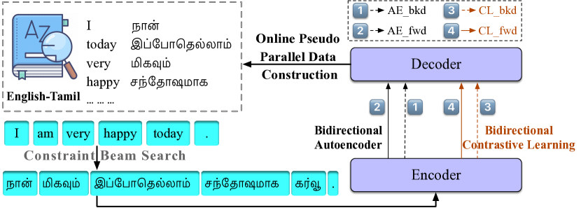
Figure 1: Method Overview. Our approach mainly consists of three parts: online constrained beam search, bidirectional autoencoder and bidirectional contrastive learning. Our approach explores the scenarios of using only target-side monolingual data and a bilingual dictionary to simultaneously alleviate the data imbalance and representation degeneration issues in large-scale MNMT model.

Although significant improvements have been made recently, we argue that there are still two major challenges to be addressed: i) MNMT models suffer from poor performance on long-tail languages (i.e., very low-resource languages), for which parallel corpora are insufficient or non-existing. We call this the data imbalance problem. For instance, $21\%$ of the language pairs in the m2m_100 model Fan et al. (2021) have a BLEU score of less than $1$ and more than $50\%$ have a BLEU score of less than $5$. Only $13\%$ have a BLEU score over $20$. For example, the average BLEU score for the language pairs with Irish as the target language is only $0.09$. ii) Degeneration of MNMT models stems from the anisotropic distribution of token representations, i.e., their representations reside in a narrow subset of the entire space (Zhang et al., 2020b). This is called the representation degeneration problem. It can lead to a prevalent issue in large-scale MNMT: the model copies sentences from the source sentence or translates them into the wrong language (off-target problem; Zhang et al., 2020a).

To address the data imbalance problem, prior work has attempted to improve the performance of a machine translation model without using any parallel data. On the one hand, unsupervised machine translation Lample et al. (2018a, b) attempts to learn models relying only on monolingual data. On the other hand, bilingual dictionaries have shown to be helpful for machine translation models Duan et al. (2020); Wang et al. (2022). What these approaches have in common is that they only require data that is both more accessible and cheaper than parallel data. As an example, 70% of the languages in the world have bilingual lexicons or word lists availableWang et al. (2022).

Representation degeneration is a prevalent problem in text generation Gao et al. (2018) and machine translation models Kudugunta et al. (2019). Contrastive learning Hadsell et al. (2006) aims to bring similar sentences in the model close together and dissimilar sentences far from each other in the representation space. This is an effective solution to the representation problem in machine translation Pan et al. (2021); Li et al. (2022). However, the naïve contrastive learning framework that utilizes random non-target sequences as negative examples is suboptimal, because they are easily distinguishable from the correct output Lee et al. (2020).

To address both problems mentioned above, we present a novel multilingual NMT approach which leverages plentiful data sources: target-side monolingual data and a bilingual dictionary. Specifically, we start by using constrained beam search Post and Vilar (2018) to construct pseudo-parallel data in an online mode. To overcome the data imbalance problem, we propose training a bidirectional autoencoder, while to address representation degeneration, we use bidirectional contrastive learning. Finally, we use a curriculum learning Bengio et al. (2009) sampling strategy. This uses the score given by token coverage in the bilingual dictionary to rearrange the order of training examples, such that sentences with more tokens in the dictionary are seen earlier and more frequently during training.

In summary, we make the following contributions: i) We propose a novel approach that uses only target-side monolingual data and a bilingual dictionary to improve MNT performance. ii) We define two modules, bidirectional autoencoder and bidirectional contrastive learning, to address the data imbalance and representation degeneration problem. iii) We show that our method demonstrates zero-shot domain transfer and language transfer capability. iv) We also show that our method is an effective solution for both the repetition Fu et al. (2021) and the off-target Zhang et al. (2020a) problems in large-scale MNMT models.

2 Related Work

Multilingual Neural Machine Translation. MNMT is rapidly moving towards developing large models that enable translation between an increasing number of language pairs. Fan et al. (2021) proposed m2m_100 model that enables translation between 100 languages. Siddhant et al. (2022) and Costa-jussà et al. (2022) extend the current MNMT models to support translation between more than 200 languages using supervised and self-supervised learning methods.

Autoencoder. An autoencoder (AE) is a generative model that is able to generate its own input. There are many variants of AE that can be useful for machine translation. Zhang et al. (2016) and Eikema and Aziz (2019) propose using a variational autoencoder to improve the performance of machine translation models. A variant of the same generative model is the denoising autoencoder, which is an important component of unsupervised machine translation models Lample et al. (2018a). However, the utility of autoencoders has not been fully explored for MNMT. To the best of our knowledge, we are the first to propose training an autoencoder using only target-side monolingual data and a bilingual dictionary to improve low-resource MNMT.

Contrastive Learning. Contrastive learning is a technique that clusters similar data together in a representation space while it simultaneously separates the representation of dissimilar sentences. It is useful for many natural language processing tasks Zhang et al. (2022). Recently, Pan et al. (2021) and Vamvas and Sennrich (2021) used contrastive learning to improve machine translation and obtained promising results. However, these methods use the random replacing technique to construct the negative examples, which often leads to a significant divergence between the semantically similar sentences and the ground-truth sentence in the model representation space. This large changes makes the model more difficult to distinguish correct sentence from incorrect ones. We use small perturbations to construct negative examples, ensuring their proximity to the ground-truth sentence within the semantic space, which significantly mitigates the aforementioned issue.

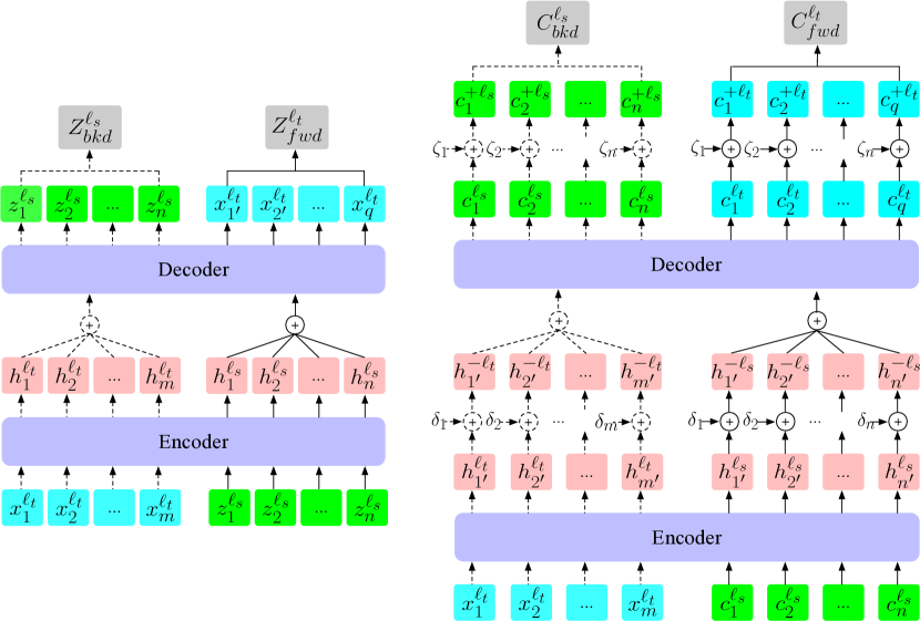
Figure 2: Model architecture: bidirectional autoencoder (left) and bidirectional contrastive learning (right). The symbols are consistent with the description in Section 3.

3 Method

Our goal is to overcome the data imbalance and representation degeneration issues in the MNMT model. We aim to improve the performance of MNMT without using parallel data, instead relying only on target-side monolingual data and a bilingual dictionary. Our approach contains three parts: online pseudo-parallel data construction (Section 3.1), bidirectional autoencoder (Section 3.2) and bidirectional contrastive learning (Section 3.3). Figure 1 illustrates the overview of our method. The architectures of the bidirectional autoencoder (left) and bidirectional contrastive learning (right) are presented in Figure 2.

3.1 Online Pseudo-Parallel Data Construction

Let us assume that we want to improve performance when translating from source language $\ell_{s}$ to target language $\ell_{t}$. We start with a monolingual set of sentences from the target language, denoted as $\mathcal{D}_{mono}^{{}^{\ell_{t}}}$, a bilingual dictionary, denoted as $\mathcal{D}_{dict}^{{\ell_{t}\rightarrow\ell_{s}}}$, and a target monolingual sentence with $tt$ tokens, denoted as $X_{i}^{\ell_{t}}=\{x_{1},...,x_{tt}\}$, $X_{i}^{\ell_{t}}\in\mathcal{D}_{mono}^{{}^{\ell_{t}}}$. We use lexically constrained decoding (i.e., constrained beam search; Post and Vilar, 2018) to generate a pseudo source language sentence $X_{i}^{\ell_{s}}=\{x_{1},...,x_{ss}\}$ in an online mode:

$$X_{i}^{\ell_{s}} =gen(X_{i}^{\ell_{s}}|\theta,X_{i}^{\ell_{t}},\mathcal{D}_{dict}^{\ell_{t}\rightarrow\ell_{s}})$$ (1)

where $gen(\cdot)$ is the lexically constrained beam search function and $\theta$ denotes the parameters of the model. It is worth noting that parameters $\theta$ will not be updated during the generation process, but will be updated in the following steps (Section 3.2 and Section 3.3).

3.2 Bidirectional Autoencoder

An autoencoder Vincent et al. (2008) first aims to learn how to efficiently compress and encode data, then to reconstruct the data back from the reduced encoded representation to a representation that is as close as possible to the original input.

We propose performing autoencoding using only target-side monolingual data. This is different from prior work on UNMT, which uses both source and target-side data Lample et al. (2018a). Our bidirectional autoencoder contains two parts: backward autoencoder (Section 3.2.1) and forward autoencoder (Section 3.2.2).

3.2.1 Backward Autoencoder

After we obtain $X_{i}^{\ell_{s}}$ from Eq. 1, we have the pseudo-parallel pairs ($X_{i}^{\ell_{t}},X_{i}^{\ell_{s}}$) $\in\mathcal{D}_{pse}$. Then, we feed $X_{i}^{\ell_{t}}$ to the MNMT model to get the contextual output embedding $\mathbf{Z_{bkd}^{\ell_{s}}}$. Formally, the encoder generates a contextual embedding $\mathbf{H}_{i}^{\ell_{t}}$ given $X_{i}^{\ell_{t}}$ and $l_{t}$ as input, which is in turn given as input to the decoder (together with $l_{s}$) to generate $\mathbf{Z_{bkd}^{\ell_{s}}}$:

$$\mathbf{H_{i}^{\ell_{t}}} =\text{Encoder}(X_{i}^{\ell_{t}},\ \ell_{t}),$$ (2)

$$\mathbf{Z_{bkd}^{\ell_{s}}} =\text{Decoder}(\mathbf{H_{i}^{\ell_{t}}},\ell_{s})$$

Finally, the backward autoencoder loss is formulated as follows:

$$\mathcal{L}_{\mathrm{AE\_bkd}}=-\sum\log P_{\theta}\left(X_{i}^{\ell_{s}}\mid X_{i}^{\ell_{t}},\mathbf{Z_{bkd}^{\ell_{s}}}\right)$$ (3)

3.2.2 Forward Autoencoder

Given $\mathbf{Z_{bkd}^{\ell_{s}}}$ from Eq. 2, we feed it to the MNMT model and get the contextual output denoted as $\mathbf{Z_{fwd}^{\ell_{t}}}$:

$$\mathbf{H_{i}^{\ell_{s}}} =\text{Encoder}(\mathbf{Z_{bkd}^{\ell_{s}}},\ \ell_{s}),$$ (4)

$$\mathbf{Z_{fwd}^{\ell_{t}}} =\text{Decoder}(\mathbf{H_{i}^{\ell_{s}}},\ \ell_{t})$$

The forward auto-encoder loss is given by:

$$\mathcal{L}_{\mathrm{AE\_fwd}}=-\sum\log P_{\theta}\left(X_{i}^{\ell_{t}}\mid\mathbf{Z_{bkd}^{\ell_{s}}},\mathbf{Z_{fwd}^{\ell_{t}}}\right)$$ (5)

3.3 Bidirectional Contrastive Learning

The main challenge in contrastive learning is to construct the positive and negative examples. Naive contrastive learning Pan et al. (2021) uses ground-truth target sentences as positive examples and random non-target sentences as negative examples. When a pretrained MNMT model is used, negative examples are initially located far from positive examples in the embedding space.

Motivated by Lee et al. (2020), we automatically generate negative and positive examples, such that both kinds of examples are difficult for the model to classify correctly. This arguably motivates learning meaningful representations. Different from Lee et al. (2020), we construct negative examples in the source-side sentence and positive examples in the target-side sentence, instead of constructing both in the target-side sentence. Specifically, to generate a negative example, we add a small perturbation $\delta_{i}=\{\delta_{1}\ldots\delta_{T}\}$ to $\mathbf{H_{{i}}}$, which is the hidden representation of the source-side sentence. We construct positive examples by adding a perturbation $\zeta_{i}=\{\zeta_{1}\ldots\zeta_{T}\}$ to $\mathbf{H_{i}}$, which is the hidden state of the target-side sentence. Different from Pan et al. (2021) who use a random replacing technique that may result in meaningless negative examples (already well-discriminated in the embedding space), we add the perturbation to ensure that the resulting embedding space is not already in a close proximity or far apart from the original embedding space. More details on how to generate the perturbation of $\delta_{i}$ and $\zeta_{i}$ can be found in Appendix A.

3.3.1 Backward Contrastive Learning

Given pseudo-parallel pairs ($X_{i^{\prime}}^{\ell_{t}},X_{i^{\prime}}^{\ell_{s}}$) $\in\mathcal{D}_{pse}$ from Eq. 1, we first feed $X_{i^{\prime}}^{\ell_{t}}$ to the MNMT model to generate the contextual embedding $\mathbf{H}_{i^{\prime}}^{\ell_{t}}$. Then, we add a small perturbation $\delta_{bkd}^{(i^{\prime})}$ after $\mathbf{H}_{i^{\prime}}^{\ell_{t}}$ to form the negative example, denoted as $\mathbf{H_{i^{\prime}}^{-\ell_{t}}}$. Finally, the contextual output of the decoder $\mathbf{C_{bkd}^{\ell_{s}}}$ is generated by feeding $H_{i^{\prime}}^{-\ell_{t}}$ to the decoder, and the positive example $\mathbf{H_{i^{\prime}}^{+\ell_{s}}}$ is generated by adding another small perturbation $\zeta_{bkd}^{(i^{\prime})}$.

$$\mathbf{H_{i^{\prime}}^{\ell_{t}}} =\text{Encoder}(X_{i^{\prime}}^{\ell_{t}},\ \ell_{t}),$$ (6)

$$\mathbf{H_{i^{\prime}}^{-\ell_{t}}} =\mathbf{H_{i^{\prime}}^{\ell_{t}}}+\delta_{bkd}^{(i^{\prime})},$$

$$\mathbf{C_{bkd}^{\ell_{s}}} =\text{Decoder}(\mathbf{H_{i^{\prime}}^{-\ell_{t}}},\ell_{s}),$$

$$\mathbf{H_{i^{\prime}}^{+\ell_{s}}} =\text{Decoder}(\mathbf{C_{bkd}^{\ell_{s}}},\ \ell_{s})+\zeta_{bkd}^{(i^{\prime})},$$

Finally, the backward contrastive learning loss is formulated as follows:

$$\mathcal{L}_{\text{CL\_bkd}}=-\sum\log\frac{e^{\text{sim}^{+}(\mathbf{H_{i^{\prime}}^{\ell_{t}}},\mathbf{H_{i^{\prime}}^{+\ell_{s}}})/\tau}}{\sum_{\mathbf{H_{i^{\prime}}^{-\ell_{t}}}}e^{\text{sim}^{-}(\mathbf{H_{i^{\prime}}^{\ell_{t}}},\mathbf{H_{i^{\prime}}^{-\ell_{t}}})/\tau}}$$ (7)

3.3.2 Forward Contrastive Learning

After we get $\mathbf{C_{bkd}^{\ell_{s}}}$ from Eq. 6, we feed $\mathbf{C_{bkd}^{\ell_{s}}}$ and the small perturbation $\mathbf{\delta_{fwd}^{(i^{\prime})}}$ to the MNMT model to obtain the contextual output denoted as $\mathbf{C_{fwd}^{\ell_{t}}}$ and the negative example $\mathbf{H_{i^{\prime}}^{-\ell_{s}}}$. Then, we feed $\mathbf{C_{fwd}^{\ell_{t}}}$ and another small perturbation $\zeta_{fwd}^{(i^{\prime})}$ to generate a positive example denoted as $\mathbf{H_{i^{\prime}}^{+\ell_{t}}}$.

$$\mathbf{H_{i^{\prime}}^{\ell_{s}}} =\text{Encoder}(\mathbf{C_{bkd}^{\ell_{s}}},\ \ell_{s}),$$ (8)

$$\mathbf{H_{i^{\prime}}^{-\ell_{s}}} =\mathbf{H_{i^{\prime}}^{\ell_{s}}}+\delta_{fwd}^{(i^{\prime})},$$

$$\mathbf{C_{fwd}^{\ell_{t}}} =\text{Decoder}(\mathbf{H_{i^{\prime}}^{-\ell_{s}}},\ell_{t}),$$

$$\mathbf{H_{i^{\prime}}^{+\ell_{t}}} =\text{Decoder}(\mathbf{C_{fwd}^{\ell_{t}}},\ \ell_{t})+\zeta_{fwd}^{(i^{\prime})},$$

Finally, the forward contrastive learning loss is given by the following equation:

$$\mathcal{L}_{\text{CL\_fwd}}=-\sum\log\frac{e^{\text{sim}^{+}(\mathbf{H_{i^{\prime}}^{\ell_{s}}},\mathbf{H_{i^{\prime}}^{+\ell_{t}}})/\tau}}{\sum_{\mathbf{H_{i^{\prime}}^{-\ell_{s}}}}e^{\text{sim}^{-}(\mathbf{H_{i^{\prime}}^{\ell_{s}}},\mathbf{H_{i^{\prime}}^{-\ell_{s}}})/\tau}}$$ (9)

3.4 Curriculum Learning

Curriculum Learning Bengio et al. (2009) suggests starting with easier tasks and progressively gaining experience to process more complex tasks, which has been proved to be useful in machine translation Stojanovski and Fraser (2019); Zhang et al. (2019); Lai et al. (2022b). In our training process, we first compute token coverage for each monolingual sentence using the bilingual dictionary. This score is used to determine a curriculum to sample the sentences for each batch, so that higher-scored sentences are selected early on during training.

3.5 Training Objective

The model can be trained by minimizing a composite loss from Eq. 3,  5,  7 and  9 as follows:

$$\mathcal{L}^{\ast}= \lambda(\mathcal{L}_{AE\_bkd}+\mathcal{L}_{AE\_fwd})+$$ (10)

$$(1-\lambda)(\mathcal{L}_{CL\_bkd}+\mathcal{L}_{CL\_fwd})$$

Where $\lambda$ is the balancing factor between the autoencoder and contrastive learning component.

4 Experiments

Datasets. We conduct three group of experiments: bilingual setting, multilingual setting and high-resource setting. In the bilingual setting, we focus on improving the performance on a specific long-tail language pair. We choose 10 language pairs at random that have $\text{BLEU}<2.5$ in the original m2m_100 model and a considerable amount of monolingual data in the target language in news-crawl. The language pairs cover the following languages (ISO 639-1 language code): en, ta, kk, ar, ca, ga, bs, ko, ka, tr, af, hi, jv, ml. In the multilingual setting, we aim to improve the performance on long-tail language pairs, which share the same target language. We randomly select 10 languages where the average BLEU score on the language pairs with the same target language is less than 2.5. For the languages not covered from news-crawl, we use the monolingual data from CCAligned El-Kishky et al. (2020). The languages we use are: ta, hy, ka, be, kk, az, mn, gu. For the high-resource setting, we aim to validate whether our proposed method also works for high-resource languages. We randomly select 6 language pairs that cover the following language codes: en, de, fr, cs.

Models	Bilingual Setting
	en$\rightarrow$ta	en$\rightarrow$kk	ar$\rightarrow$ta	ca$\rightarrow$ta	ga$\rightarrow$bs	kk$\rightarrow$ko	ka$\rightarrow$ar	ta$\rightarrow$tr	af$\rightarrow$ta	hi$\rightarrow$kk
m2m	2.12	0.26	0.34	1.75	0.51	0.85	2.14	1.41	1.46	0.84
pivot_en	-	-	0.30	0.74	0.00	0.27	0.15	1.38	1.00	0.22
BT	0.76	0.67	0.60	1.13	0.63	0.97	0.06	2.05†	0.72	0.43
wbw_lm	2.76†	0.36	0.87	0.68	0.36	0.07	2.86†	2.26†	1.47	0.04
syn_lexicon	1.33	0.14	0.72	2.07†	0.93	1.10†	0.85	0.57	2.07†	0.89
Bi-ACL w/o Curriculum	4.57‡	1.35‡	1.76‡	3.14‡	1.81‡	3.07‡	3.92‡	4.18‡	3.15‡	1.53‡
Bi-ACL (ours)	5.14‡	2.59‡	2.32‡	3.50‡	2.37‡	3.61‡	4.76‡	4.97‡	3.68‡	2.47‡
$\Delta$	+3.02	+2.33	+1.98	+1.75	+1.86	+3.03	+2.62	+3.56	+2.22	+1.63
	Multilingual Setting
	ta	hy	ka	be	kk	az	mn	gu	my	ga
m2m	1.46	1.69	0.52	1.95	0.67	2.32	1.12	0.26	0.24	0.09
Bi-ACL	2.54‡	3.17‡	2.38‡	3.12‡	1.44‡	3.28‡	1.95‡	1.18‡	1.94‡	1.37‡
$\Delta$	+1.08	+1.48	+1.86	+1.17	+0.77	+0.96	+0.83	+0.92	+1.70	+1.28
	Multilingual Setting (specific language pair)
	en$\rightarrow$ta∗	ar$\rightarrow$ta∗	ca$\rightarrow$ta∗	af$\rightarrow$ta∗	el$\rightarrow$ta	en$\rightarrow$kk∗	hi$\rightarrow$kk∗	fa$\rightarrow$kk	jv$\rightarrow$kk	ml$\rightarrow$kk
m2m	2.12	0.34	1.75	1.46	1.21	0.26	0.84	0.54	1.77	0.69
Bi-ACL	5.37‡	2.81‡	3.82‡	4.16‡	3.24‡	2.94‡	2.91‡	2.87‡	3.73‡	3.29‡
$\Delta$	+3.25	+2.47	+2.07	+2.70	+2.03	+2.68	+2.07	+2.33	+1.96	+2.60
$\Phi$	+0.23	+0.49	+0.32	+0.48	-	+0.35	+0.44	-	-	-

Table 1: Main Results: BLEU scores for low-resource language pairs in the bilingual, multilingual setting, and 10 randomly selected language pairs in the multilingual setting. Language pairs with ^∗ in the multilingual setting are covered by the bilingual setting. $\Delta$ denotes improvement over the original m2m_100 model, while $\Phi$ shows improvement over the bilingual setting. Best results are shown in bold. ^† and ^‡ denotes significant over original m2m_100 model at 0.05/0.01, evaluated by bootstrap resampling Koehn (2004).

Dictionaries. We extract bilingual dictionaries using the wiktextextract tool. For pairs not involving English, we pivot through English. Given a source language $\ell_{s}$ and a target language $\ell_{t}$, the intersection of the two respective bilingual dictionaries with English creates a bilingual dictionary $\mathcal{D}_{dict}^{\ell_{s}\rightarrow\ell_{t}}$ from $\ell_{s}$ to $\ell_{t}$. The statistics of the dictionaries can be seen in Appendix D.1.

Data Preprocessing. For the monolingual data, we first use a language detection tool (langid) to filter out sentences with mixed language. We proceed to remove the sentences containing at least 50% punctuation and filter out duplicated sentences. To control the influence of corpus size on our experimental results, we limit the monolingual data of all languages to 1M. For dictionaries, we also use langid to filter out the wrong languages both on the source and target side.

Baselines. We compare our methods to the following baselines: i) m2m: Using the original m2m_100 model Fan et al. (2021) to generate translations. ii) pivot_en: Using English as a pivot language, we leverage m2m_100 to translate target-side monolingual data to English and then translate English to the source language. Following this method, we finetune the m2m_100 model using the pseudo-parallel data. iii) BT: Back-Translate Sennrich et al. (2016) target-side monolingual data using m2m_100 model to generate the pseudo source-target parallel dataset, then finetune the m2m_100 model using this data. iv) wbw_lm: Use a bilingual dictionary, cross-lingual word embeddings and a target-side language model to translate word-by-word and then improve the translation through a target-side denoising model Kim et al. (2018). v) syn_lexicon: Replace the words in the target monolingual sentence with the corresponding source language words in a bilingual dictionary and use the pseudo-parallel data to finetune the m2m_100 model Wang et al. (2022).

Implementation. We use m2m, released in the HuggingFace repository Wolf et al. (2020). For the wbw_lm baseline, monolingual word embeddings are directly obtained from the fasttext website and cross-lingual embeddings are trained using a bilingual dictionary as a supervision signal. We set $\lambda=0.7$ in all our experiments (the effect of different $\lambda$ can be find in Appendix E.5).

Evaluation. We measure case-sensitive detokenized BLEU and statistical significant testing as implemented in SacreBLEU All results are computed on the devtest dataset of Flores101 Goyal et al. (2022). To evaluate the isotropy of the MNMT model, we adopt the $I_{1}$ and $I_{2}$ isotropy measures from Wang et al. (2019), with $I_{1}(\mathbf{W})\in[0,1]$ and $I_{2}(\mathbf{W})\geq 0$, where $\mathbf{W}$ is the model matrix from the whole model parameter $\theta$. Larger $I_{1}(\mathbf{W})$ and smaller $I_{2}(\mathbf{W})$ indicate a more isotropic embedding space in the MNMT model. Please refer to Appendix B for more details on $I_{1}$ and $I_{2}$.

	ar$\rightarrow$ta				ta$\rightarrow$tr				de$\rightarrow$fr
	Encoder		Decoder		Encoder		Decoder		Encoder		Decoder
	$I_{1}\uparrow$	$I_{2}\downarrow$	$I_{1}\uparrow$	$I_{2}\downarrow$	$I_{1}\uparrow$	$I_{2}\downarrow$	$I_{1}\uparrow$	$I_{2}\downarrow$	$I_{1}\uparrow$	$I_{2}\downarrow$	$I_{1}\uparrow$	$I_{2}\downarrow$
m2m	0.042	20.017	0.012	26.639	0.036	20.408	0.006	26.901	0.058	16.521	0.016	24.695
pivot_en	0.034	22.852	0.008	24.472	0.019	22.889	0.007	25.977	0.056	16.843	0.016	24.763
BT	0.011	25.825	0.007	25.797	0.028	22.009	0.009	27.492	0.074	14.774	0.015	24.878
wbw_lm	0.023	23.485	0.015	24.746	0.038	19.389	0.010	26.320	0.037	19.099	0.015	24.935
syn_lexicon	0.059	17.513	0.015	25.694	0.028	20.640	0.013	26.475	0.020	23.859	0.014	24.137
Bi-ACL w/o Curriculum	0.074	16.174	0.017	24.176	0.039	19.139	0.018	24.712	0.078	14.165	0.017	24.128
Bi-ACL (ours)	0.086	15.714	0.020	23.251	0.043	18.672	0.021	22.716	0.086	13.666	0.017	24.067

Table 2: Main Results: Isotropic embedding space analysis in ar$\rightarrow$ta and ta$\rightarrow$tr translation task. The definitions of $I_{1}$ and $I_{2}$ can be found in Appendix B.

Models	en$\rightarrow$de	en$\rightarrow$fr	en$\rightarrow$cs	de$\rightarrow$fr	de$\rightarrow$cs	fr$\rightarrow$cs
m2m	22.79	32.50	21.65	28.53	20.73	20.30
pivot_en	-	-	-	11.68	7.09	6.60
BT	24.08	27.71	21.52	19.45	17.41	17.00
wbw_lm	7.52	11.53	9.04	8.38	9.44	10.15
syn_lexicon	5.35	12.56	10.90	5.90	8.39	8.89
Bi-ACL w/o Curriculum	25.17	35.52	23.91	29.43	22.71	22.04
Bi-ACL (ours)	27.76	37.84	25.89	30.66	23.80	23.56
$\Delta$	+4.97	+5.34	+4.24	+2.13	+3.07	+3.26

Table 3: Main Results: BLEU scores for high-resource language pairs in the bilingual setting.

5 Results

Table 1 shows the main results on low-resource language pairs in a bilingual and multilingual setting. Table 3 shows results on high-resource language-pairs in a bilingual setting, while Table 2 presents an isotropic embedding space analysis for the bilingual setting.

Low-Resource Language Pairs in a Bilingual Setting. As shown in Table 1, the baselines perform poorly and several of them are worse than the original m2m_100 model. This can be attributed to the fact that their performance depends on the translation quality in the direction of source language to English and English to target language (pivot_en), the quality in the reverse direction (BT), the quality of cross-lingual word-embeddings (wbw_lm) and the token coverage in bilingual dictionary (syn_lexicon). Our method outperforms the baselines across all language pairs, even when the performance of the language pair is poor in the original m2m_100 model. In addition, using the curriculum learning sampling strategy further improves our model’s performance.

Low-Resource Language Pairs in a Multilingual Setting. In the middle part of Table 1, we show the average BLEU scores of all language pairs with the same target language. Our approach consistently shows promising results across all languages. Based on the results shown in the lower part of the same Table, we notice that the BLEU scores obtained in the multilingual setting on a specific language pair outperform the scores obtained in the bilingual setting. For example, we get 3.68 BLEU points for af$\rightarrow$ta in the bilingual setting, while we get 4.16 in the multilingual setting. This confirms our intuition that knowledge transfer between different languages in the MNMT model when using a multilingual setting is beneficial (see more details in Section 6.2).

High-Resource Language Pairs in a Bilingual Setting. As shown in Table 3, baseline systems do not perform well on all high-resource pairs due to the same reasons as in the long-tail languages setting. Our approach outperforms the baselines on all high-resource pairs. In addition, curriculum learning takes full advantage of the original model in the high-resource setting, with stronger gains in performance than in the low-resource setting. Interestingly, our findings reveal that back translation does not yield optimal results in both low and high resource settings. In low-resource languages, the performance of the language pair and its reverse direction in the original m2m_100 model is significantly poor (i.e., nearly zero). Consequently, the use of back-translation results in a performance that is inferior to that of m2m_100. For high-resource languages, the language pairs already exhibit strong performance in the original m2m_100 model. This makes it challenging to demonstrate that the incorporation of additional pseudo-parallel data can outperform the non-utilization of the pseudo-corpus. Another potential concern is that the large amount of monolingual data we employ, coupled with the substantial amount of pseudo-parallel data derived from back translation, may disrupt the pre-trained model. This observation aligns with the findings of Liao et al. (2021) and Lai et al. (2021).

	$\mathcal{L}_{AE\_bkd}$	$\mathcal{L}_{AE\_fwd}$	$\mathcal{L}_{CL\_bkd}$	$\mathcal{L}_{CL\_fwd}$	en$\rightarrow$ta			ta$\rightarrow$tr			en$\rightarrow$de
					BLEU	$I_{1}\uparrow$	$I_{2}\downarrow$	BLEU	$I_{1}\uparrow$	$I_{2}\downarrow$	BLEU	$I_{1}\uparrow$	$I_{2}\downarrow$
#1	$\surd$	$\times$	$\times$	$\times$	2.51	0.005	30.737	3.34	0.004	32.378	23.14	0.011	24.876
	$\times$	$\surd$	$\times$	$\times$	3.27	0.006	29.299	3.96	0.006	29.373	23.82	0.011	24.651
	$\times$	$\times$	$\surd$	$\times$	2.39	0.008	26.562	2.69	0.007	28.663	22.57	0.013	24.872
	$\times$	$\times$	$\times$	$\surd$	2.36	0.009	26.541	2.65	0.007	27.155	22.89	0.013	24.367
#2	$\surd$	$\surd$	$\times$	$\times$	4.03	0.009	27.147	4.12	0.011	27.039	25.62	0.014	24.075
	$\surd$	$\times$	$\surd$	$\times$	2.36	0.012	26.782	3.64	0.010	27.636	24.84	0.013	24.513
	$\surd$	$\times$	$\times$	$\surd$	2.50	0.014	26.007	3.37	0.012	26.881	24.36	0.012	24.841
	$\times$	$\surd$	$\surd$	$\times$	3.54	0.012	26.964	3.89	0.011	27.175	24.59	0.012	24.764
	$\times$	$\surd$	$\times$	$\surd$	3.81	0.019	25.597	4.03	0.015	26.460	25.17	0.014	24.025
	$\times$	$\times$	$\surd$	$\surd$	2.53	0.013	28.459	3.61	0.012	27.639	24.73	0.012	24.723
#3	$\surd$	$\surd$	$\surd$	$\times$	3.85	0.020	24.732	3.73	0.016	26.197	25.43	0.014	24.137
	$\surd$	$\surd$	$\times$	$\surd$	4.31	0.028	23.861	4.29	0.019	25.573	26.44	0.015	24.019
	$\surd$	$\times$	$\surd$	$\surd$	2.82	0.023	24.352	3.77	0.018	25.852	25.63	0.014	24.257
	$\times$	$\surd$	$\surd$	$\surd$	3.83	0.025	24.173	4.05	0.015	26.447	26.17	0.015	14.192
#4	$\surd$	$\surd$	$\surd$	$\surd$	5.14	0.031	22.392	4.97	0.022	24.175	27.76	0.016	23.951

Table 4: Ablation study of four loss functions on en$\rightarrow$ta and ta$\rightarrow$ar translation task. “$\surd$” means the loss function is included in the training objective while “$\times$” means it is not. Both $I_{1}$ and $I_{2}$ score are computed in the decoder side.

Statistical Significance Tests. The use of BLEU in isolation as the single metric for evaluating the quality of a method has recently received criticism Kocmi et al. (2021). Therefore, we conduct statistical significance testing in the low-resource setting to demonstrate the difference as well as the superiority of our method over other baseline systems. As can be seen in Table 1, our method outperforms the baseline by significant differences, which is even more evident in the case study in Table 10. This is because the baseline system faces the serious problems of generating duplicate words (repeat problem) and translating to the wrong language (off-target problem), while our method avoids these two problems.

Isotropy Analysis. It is clear from Table 2 that the embedding space on the encoder side is more isotropic than on the decoder side. This is because we only use the target-side monolingual data to improve the decoder of the MNMT model. Compared to other baseline systems, we get a higher $I_{1}$ and lower $I_{2}$ score, which shows a more isotropic embedding space in our methods. An interesting finding is that the difference in isotropic space between high-resource language pairs is not significant. This phenomenon is because the original m2m_100 model already performs very well on high-resource language pairs and the representation degeneration is not substantial for those language pairs. In addition, the phenomenon is consistent with the findings in Table 4.

6 Analysis

In this section, we conduct additional experiments to better understand the strengths of our proposed methods. We first investigate the impact of four components on the results through an ablation study (Section 6.1). Then, we evaluate the zero-shot domain transfer ability and language transfer ability of our method (Section 6.2). Finally, we evaluate some impact factors (the quality of bilingual dictionary and the amount of monolingual data) on our proposed method (Section 6.3) and present a case study to show the strengths of our approach in solving the repetition problem and off-target issues in MNMT model.

6.1 Ablation Study

Our training objective function, shown in Eq. 10, contains four loss functions. We perform an ablation study on en$\rightarrow$ta, ta$\rightarrow$ar and en$\rightarrow$de translation tasks to understand the contribution of each loss function. The experiments in Table 4 are divided into four groups, each group representing the number of loss functions. We have the following three findings: i) #1 clearly shows that the bidirectional autoencoder losses ($\mathcal{L}_{AE\_bkd}$ and $\mathcal{L}_{AE\_fwd}$) play a more critical role than the bidirectional contrastive learning losses ($\mathcal{L}_{CL\_bkd}$ and $\mathcal{L}_{CL\_fwd}$) in terms of BLEU score. However, bidirectional contrastive losses are more important than bidirectional autoencoder losses in terms of $I_{1}$ and $I_{2}$ score. This could be the case because contrastive learning aims to improve the MNMT model’s isotropic embedding space rather than the translation from source language to target language. ii) Using forward direction losses results in a better translation quality compared to backward direction losses (#1). This is because our goal is to improve the performance from source language to target language, which is the forward direction in the loss functions. iii) The more loss functions there are, the better the performance. The combination of all four loss functions yields the best performance. iv) We show that the $I_{1}$ and $I_{2}$ scores in high-resource language pairs (en$\rightarrow$de) do not have a significant change as the original embedding space is already isotropic.

6.2 Domain Transfer and Language Transfer

Motivated by recent work on the domain and language transfer ability of MNMT models Lai et al. (2022a), we conduct a number of experiments with extensive analysis to validate the zero-shot domain transfer ability, as well as the language transfer ability of our proposed method. We have the following findings: i) Our proposed method works well not only on the Flores101 datasets (domains similar to training data of the original m2m_100 model), but also on other domains. This supports the domain transfer ability of our proposed method. ii) We show that the transfer ability is more obvious in the multilingual setting than in the bilingual setting, which is consistent with the conclusion from Table 6 in the multilingual setting. More details can be found in Appendix E.3 and E.4.

6.3 Further Investigation

To investigate two other important factors in our proposed methods, we conducted additional experiments to evaluate the impact of the quality of the dictionary and the amount of monolingual data. In general, we observe that better performance can be obtained by utilizing a high-quality bilingual dictionary. In addition, the size of the monolingual data used is not proportional to the performance improvement. More details can be found in Appendix E.1 and E.2. Also, compared with the baseline models, our method has strengths in solving repetition and off-target problems, which are two common issues in large-scale MNMT models. More details can be found in Appendix E.6.

7 Conclusion

To address the data imbalance and representation degeneration problem in MNMT, we present a framework named Bi-ACL which improves the performance of MNMT models using only target-side monolingual data and a bilingual dictionary. We employ a bidirectional autoencoder and bidirectional contrastive learning, which prove to be effective both on long-tail languages and high-resource languages. We also find that Bi-ACL shows language transfer and domain transfer ability in zero-shot scenarios. In addition, Bi-ACL provides a paradigm that an inexpensive bilingual lexicon and monolingual data should be fully exploited when there are no bilingual parallel corpora, which we believe more researchers in the community should be aware of.

8 Limitations

This work has two main limitations. i) We only evaluated the proposed method on the machine translation task, however, Bi-ACL should work well on other NLP tasks, such as text generation or question answering task, because our framework only depends on the bilingual dictionary and monolingual data, which can be easily found on the internet for many language pairs. ii) We only evaluated Bi-ACL using m2m_100 as a pretrained model. However, we believe that our approach would also work with other pretrained models, such as mT5 Xue et al. (2021) and mBART Liu et al. (2020). Because the two components (bidirectional autoencoder and bidirectional contrastive learning) we proposed can be seen as plugins, they could be easily added to any pretrained model.

	en$\rightarrow$ta				ka$\rightarrow$ar				ta$\rightarrow$tr
	Flores	TED	QED	KDE	Flores	TED	QED	KDE	Flores	TED	QED	KDE
m2m	2.12	2.19	1.16	0.57	2.14	4.47	1.00	13.35	1.41	2.03	1.32	8.10
pivot_en	-	-	-	-	0.15	0.21	0.08	0.53	1.38	1.34	0.86	3.93
BT	0.76	0.26	0.01	0.36	0.06	0.24	0.09	0.64	2.05	0.89	0.63	2.81
wbw_lm	2.76	1.97	0.29	0.67	2.86	0.17	0.12	6.24	2.26	1.53	1.19	8.70
syn_lexicon	1.33	1.19	0.08	0.20	0.85	1.65	0.45	10.64	0.57	0.41	0.55	7.08
Bi-ACL w/o Curriculum	4.57	2.62	1.24	0.75	3.92	4.61	1.20	13.82	4.18	2.39	1.68	11.75
Bi-ACL	5.14	2.84	1.41	1.05	4.76	4.93	1.57	14.62	4.97	2.81	1.96	12.74
$\Delta$	+3.02	+0.65	+0.25	+0.48	+2.62	+0.46	+0.57	+1.27	+3.56	+0.78	+0.64	+4.64

Table 5: Domain transfer: BLEU scores on en$\rightarrow$ta, ka$\rightarrow$ar, ta$\rightarrow$tr in different domains.

	Bilingual Setting
	en2ta$\Rightarrow$ar2ta	ar2ta$\Rightarrow$en2ta
m2m	0.34	2.12
pivot_en	-	0.34
BT	0.28	0.55
wbw_lm	1.07	2.68
syn_lexicon	0.43	1.86
Bi-ACL w/o curriculum	2.08	4.53
Bi-ACL transfer	2.74	5.78
$\Phi$	+0.42	+0.64
	Multilingual Setting
	ta$\Rightarrow$be	be$\Rightarrow$ta
m2m	1.95	1.46
Bi-ACL	2.73	2.31
Bi-ACL transfer	3.67	3.42
$\Phi$	+0.55	+0.88

Table 6: Language transfer: BLEU scores on langauge (pair) transfer ablity both on bilingual setting and multilingual setting. ‘A$\Rightarrow$B’ means from language (pair) A transfer to language (pair) B. $\Phi$ denotes the improvement on our proposed methods.

Appendix A Contrastive Learning

Our approach is different from traditional contrastive learning, which takes a ground-truth sentence pair as a positive example and a random non-target sentence pair in the same batch as a negative example. Motivated by Lee et al. (2020), we construct positive and negative examples automatically.

A.1 Negative Example Formulation

As described in Section 3.3, to generate a negative example, we add a small perturbation $\delta_{i}=\{\delta_{1}\ldots\delta_{T}\}$ to the $\mathbf{H_{{i}}}$, which is the hidden representation of the source-side sentence. As seen in Eq. 6, the negative example is denoted as $\mathbf{H_{i^{\prime}}^{-\ell_{t}}}$, and is formulated as the sum of the original contextual embedding $\mathbf{H_{i^{\prime}}^{\ell_{t}}}$ of the target language sentence $X_{i^{\prime}}^{\ell_{t}}$ and the perturbation $\delta_{bkd}^{(i^{\prime})}$. Finally, $\delta_{bkd}^{(i^{\prime})}$ is formulated as the conditional log likelihood with respect to $\mathbf{\delta}$. $\delta_{bkd}^{(i^{\prime})}$ is semantically very dissimilar to $X_{i^{\prime}}^{\ell_{t}}$, but very close to the hidden representation $\mathbf{H_{i^{\prime}}^{-\ell_{t}}}$ in the embedding space.

$$\mathbf{H_{i^{\prime}}^{\ell_{t}}} =\text{Encoder}(X_{i^{\prime}}^{\ell_{t}},\ \ell_{t}),$$

$$\mathbf{H_{i^{\prime}}^{-\ell_{t}}} =\mathbf{H_{i^{\prime}}^{\ell_{t}}}+\delta_{bkd}^{(i^{\prime})}$$

$$\delta_{bkd}^{(i^{\prime})} =\underset{\boldsymbol{\delta},\|\boldsymbol{\delta}\|_{2}\leq\epsilon}{\arg\min}\log p_{\theta}\left(X_{i^{\prime}}^{\ell_{s}}\mid X_{i^{\prime}}^{\ell_{t}};\mathbf{H_{i^{\prime}}^{\ell_{t}}}+\boldsymbol{\delta}\right)$$

where $\epsilon\in(0,1]$ is a parameter that controls the perturbation and $\theta$ denotes the parameters of the MNMT model.

A.2 Positive Example Formulation

As shown in Eq. 6, we create a positive example of the target sentence by adding a perturbation $\zeta_{i}=\{\zeta_{1}\ldots\zeta_{T}\}$ to $\mathbf{H_{i}}$, which is the hidden state of the target-side sentence. The objective of the perturbation $\zeta_{bkd}^{(i^{\prime})}$ is to minimize the KL divergence between the perturbed conditional distribution and the original conditional distribution as follows:

where $\theta^{*}$ is the copy of the model parameter $\theta$. As a result, the positive example is semantically similar to $X_{i^{\prime}}^{\ell_{s}}$ and dissimilar to the contextual embedding of the target sentence in the embedding space.

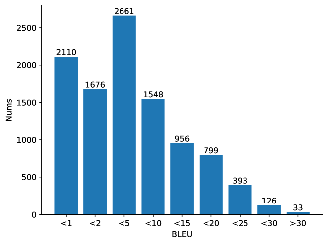
Figure 3: BLEU score statistics of the m2m_100 model Fan et al. (2021) on Flores101 dataset Goyal et al. (2022) for $102\times 101=10302$ language pairs. Each bar denotes the number of language pairs in the interval of the BLEU score.

Appendix B Evaluation of Isotropy

We use $I_{1}$ and $I_{2}$ scores from Wang et al. (2019) to characterize the isotropy of the output embedding space.

$$I_{1}(\boldsymbol{W}) =\frac{\min_{\boldsymbol{s}\in\boldsymbol{S}}Z(\boldsymbol{s})}{\max_{\boldsymbol{s}\in\boldsymbol{S}}Z(\boldsymbol{s})}$$

$$I_{2}(\boldsymbol{W}) =\sqrt{\frac{\sum_{\boldsymbol{s}\in\boldsymbol{S}}(Z(\boldsymbol{s})-\bar{Z}(\boldsymbol{s}))^{2}}{|S|\bar{Z}(\boldsymbol{s})^{2}}}$$

where $Z(\boldsymbol{s})=\sum_{i=1}^{n}\exp\left(\boldsymbol{s}^{T}\boldsymbol{w}_{i}\right)$ is close to some constant with high probability for all unit vectors $\boldsymbol{s}$ if the embedding matrix $\boldsymbol{W}$ is isotropic ($\boldsymbol{w_{i}}\in\boldsymbol{W}$). $\boldsymbol{S}$ is the set of eigenvectors of $\mathbf{W}^{\top}\mathbf{W}$. $I_{2}$ is the sample standard deviation of $Z(\boldsymbol{s})$ normalized by its average $\bar{Z}(\boldsymbol{s}))$. We have $I_{1}(\boldsymbol{W})\in[0,1]$ and $I_{2}(\boldsymbol{W})\geq 0$. Larger $I_{1}(\boldsymbol{W})$ and smaller $I_{2}(\boldsymbol{W})$ indicate more isotropic for word embedding space.

In this work, we randomly select 128 sentences from Flores101 benchmark to compute these two criteria. The results are shown in Table 2.

Appendix C Model Configuration

We use the m2m_100 model with 418MB parameters implemented in Huggingface. In our experiments, we use the AdamW Loshchilov and Hutter (2018) optimizer and the learning rate are initial to $2e-5$ with a dropout probability $0.1$. We trained our models on one machine with 4 NVIDIA V100 GPUs. The batch size is set to 8 per GPU during training. To have a fair comparison, all experiments are trained for 3 epochs.

Appendix D Statistics

D.1 Statistics of BLEU scores in m2m_100

Figure 3 shows the BLEU scores of the m2m_100 model on all $10302$ supported language pairs. We see that 21% of the langauge pairs have a BLEU score of almost $0$ and more than 50% have a BLEU score of less than $5$.

D.2 Statistics of Bilingual Dictionaries

Table 7 shows the size of the bilingual dictionaries used in a bilingual setting. For the multilingual setting, we will publish our code to generate the bilingual dictionary for any language pair.

Language Pair	#Size	Language Pair	#Size
en$\rightarrow$ta	8,376	af$\rightarrow$ta	5,268
en$\rightarrow$kk	11,323	hi$\rightarrow$kk	24,762
ar$\rightarrow$ta	26,768	en$\rightarrow$de	68,029
ca$\rightarrow$ta	18,757	en$\rightarrow$fr	78,837
ga$\rightarrow$bs	125,336	en$\rightarrow$cs	35,879
kk$\rightarrow$ko	38,710	de$\rightarrow$fr	207,831
ka$\rightarrow$ar	25,825	de$\rightarrow$cs	125,909
ta$\rightarrow$tr	14,169	fr$\rightarrow$cs	104,510

Table 7: Statistics of bilingual dictionaries.

	en$\rightarrow$ta	ca$\rightarrow$ta	ga$\rightarrow$bs	ta$\rightarrow$tr
m2m	2.12	1.75	0.51	1.41
panlex	3.19	2.47	0.67	3.41
wiktionary	5.14	3.50	2.37	4.97

Table 8: The effect of bilingual dictionary quality on experimental performance in terms of BLEU score.

	en$\rightarrow$ta	en$\rightarrow$kk	ar$\rightarrow$ta	ca$\rightarrow$ta
m2m	2.12	0.26	0.34	1.75
$\phi=0.5$	3.70	0.84	1.22	2.28
$\phi=0.6$	3.60	0.75	1.07	2.26
$\phi=0.7$	3.64	0.23	1.15	2.24
$\phi=0.8$	3.82	0.46	1.28	2.52
$\phi=0.9$	5.14	2.59	2.32	3.50
$\phi=1.0$	3.27	0.07	1.01	2.15

Table 9: The effect of monolingual corpus size in experimental results in terms of BLEU score. The smaller the value of $\phi$ (bilingual dictionary coverage) the larger the monolingual corpus.

Table 10: Case study

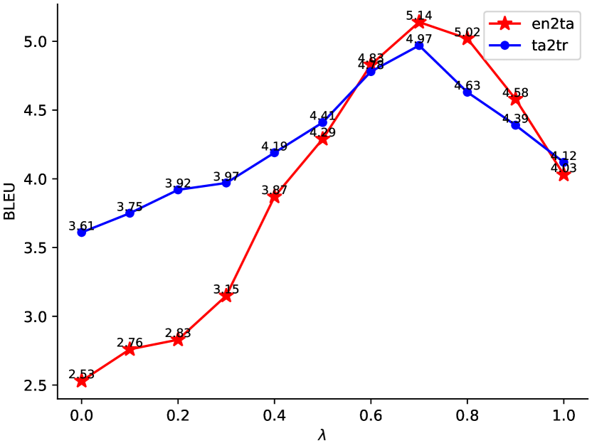
(a) Long-Tail Language Pair

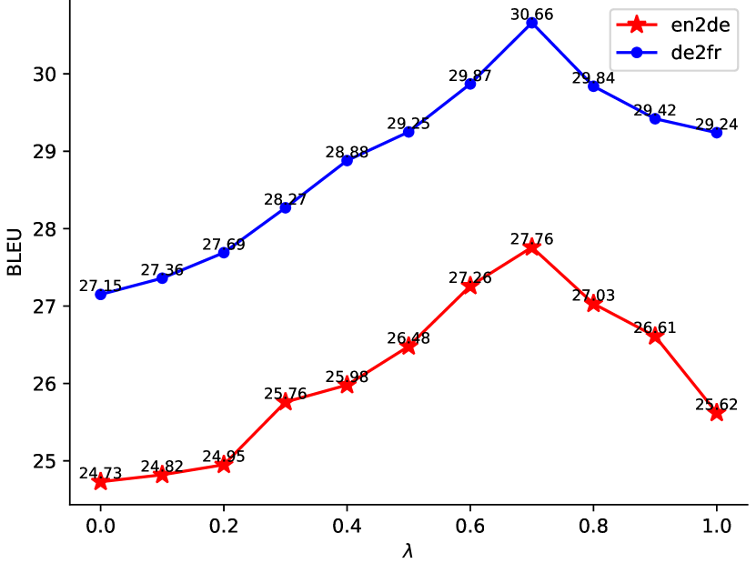
(b) High-Resource Language Pair

Figure 4: The effect of different $\lambda$

Appendix E Further Analysis

E.1 Quality of the Bilingual Dictionary

To investigate whether the quality of bilingual dictionary affects the performance of our method, we conduct additional experiments using the Panlex dictionary, a big dataset that covers 5,700 languages. We evaluate the performance on en$\rightarrow$ta, ca$\rightarrow$ta, ga$\rightarrow$bs and ta$\rightarrow$tr translation tasks.

As seen in Table 8, using the dictionary mined from wikitionary results in a better performance than using the panlex dictionary. The reason for this is that, while Panlex supports bilingual dictionaries for many language pairs, we discovered that the quality of them is quite low, especially when English is not one of the two languages in the language pair.

E.2 Amount of Monolingual Data

As described in Section 3.4, we use the bilingual dictionary coverage $\phi$ as the curriculum to order the training batch. In this section, we aim to investigate how the number of monolingual data affects the experimental results. A smaller $\phi$ means a larger number of monolingual data. We conduct experiments on en$\rightarrow$ta, en$\rightarrow$kk, ar$\rightarrow$ta and ca$\rightarrow$ta translation tasks with a different $\phi$.

As seen in Table 9, we observe that the amount of monolingual data is not proportional to the experimental performance. This is because a large percentage of words in a sentence are not covered by lexicons in the bilingual dictionaries, the performance of constrained beam search is limited. This phenomenon is consistent with the conclusion that the effect of the size of the pseudo parallel corpus in data augmentation Fadaee et al. (2017) and back-translation  Sennrich et al. (2016) on the experimental results, i.e., that the performance of machine translation is not proportional to the size of the pseudo parallel corpus.

E.3 Domain Transfer

To investigate the domain transfer ability of our approach, we first conduct experiments on en$\rightarrow$ta, ka$\rightarrow$ar, ta$\rightarrow$tr translation tasks, then evaluate the performance in a zero-shot setting on three different domains (TED, QED and KDE) which are publicly available datasets from OPUS Tiedemann (2012) and on the Flores101 benchmark. The results is shown in Table 5.

According to Table 5, the performance of the baseline systems is even worse than the original m2m_100 model, which suggests that they do not show domain robustness nor domain transfer ability due to poor performance (see Table 1). In contrast, our proposed method works well not only on the Flores101 datasets (domains similar to training data of the original m2m_100 model), but also on other domains.

E.4 Language Transfer

To investigate the language transfer ability, we use the model trained on a specific language (pair) to generate text for another language (pair) both in the bilingual and multilingual settings. For the bilingual setting, we run experiments to assess the language transfer ability between en$\rightarrow$ta and ar$\rightarrow$ta translation tasks. For the multilingual setting, we focus on translation scores between ta and be. The results is shown in Table 6.

As indicated in Table 6, we observe that the performance in our method outperforms the other baselines both in the bilingual and in the multilingual setting. We also discover that the transfer ability is more obvious in the multilingual setting than in the bilingual setting. This phenomenon is consistent with the conclusion from Table 1 in the multilingual setting. We believe that this can be attributed to the fact that in a multilingual setting, the language is used for all language pairs that share the same target language, which can be seen as common information for all language pairs.

E.5 The effect of $\lambda$

In Section 3.5, we set a $\lambda$ to balance the importance of both autoencoding and contrastive loss to our model. From Figure 4, we show that the autoencoding loss plays a more important role than contrastive loss in terms of BLEU. When $\lambda=0.7$, we got the best performance both in long-tail language pair and high-resource langauge pair.

E.6 Case Study

We now present qualitative results on how our method addresses the repetition and off-target problems. For the first example in Figure 10, we find that other baseline systems suffer from a severe repetition problem. This is attributed to a poor decoder. In contrast, our method does not have a repetition problem, most likely because we enhanced the representation of the decoder through a bidirectional contrastive loss. For the second example, we show that while the off-target problem is prevalent in baseline systems, our method seems to provide an effective solution to it.

References

- Aharoni et al. (2019) Roee Aharoni, Melvin Johnson, and Orhan Firat. 2019. Massively multilingual neural machine translation. In Proceedings of the 2019 Conference of the North American Chapter of the Association for Computational Linguistics: Human Language Technologies, Volume 1 (Long and Short Papers), pages 3874–3884, Minneapolis, Minnesota. Association for Computational Linguistics.
- Bengio et al. (2009) Yoshua Bengio, Jérôme Louradour, Ronan Collobert, and Jason Weston. 2009. Curriculum learning. In Proceedings of the 26th annual international conference on machine learning, pages 41–48.
- Costa-jussà et al. (2022) Marta R Costa-jussà, James Cross, Onur Çelebi, Maha Elbayad, Kenneth Heafield, Kevin Heffernan, Elahe Kalbassi, Janice Lam, Daniel Licht, Jean Maillard, et al. 2022. No language left behind: Scaling human-centered machine translation. arXiv preprint arXiv:2207.04672.
- Duan et al. (2020) Xiangyu Duan, Baijun Ji, Hao Jia, Min Tan, Min Zhang, Boxing Chen, Weihua Luo, and Yue Zhang. 2020. Bilingual dictionary based neural machine translation without using parallel sentences. In Proceedings of the 58th Annual Meeting of the Association for Computational Linguistics, pages 1570–1579, Online. Association for Computational Linguistics.
- Eikema and Aziz (2019) Bryan Eikema and Wilker Aziz. 2019. Auto-encoding variational neural machine translation. In Proceedings of the 4th Workshop on Representation Learning for NLP (RepL4NLP-2019), pages 124–141, Florence, Italy. Association for Computational Linguistics.
- El-Kishky et al. (2020) Ahmed El-Kishky, Vishrav Chaudhary, Francisco Guzmán, and Philipp Koehn. 2020. CCAligned: A massive collection of cross-lingual web-document pairs. In Proceedings of the 2020 Conference on Empirical Methods in Natural Language Processing (EMNLP), pages 5960–5969, Online. Association for Computational Linguistics.
- Fadaee et al. (2017) Marzieh Fadaee, Arianna Bisazza, and Christof Monz. 2017. Data augmentation for low-resource neural machine translation. In Proceedings of the 55th Annual Meeting of the Association for Computational Linguistics (Volume 2: Short Papers), pages 567–573, Vancouver, Canada. Association for Computational Linguistics.
- Fan et al. (2021) Angela Fan, Shruti Bhosale, Holger Schwenk, Zhiyi Ma, Ahmed El-Kishky, Siddharth Goyal, Mandeep Baines, Onur Celebi, Guillaume Wenzek, Vishrav Chaudhary, et al. 2021. Beyond english-centric multilingual machine translation. Journal of Machine Learning Research, 22(107):1–48.
- Fu et al. (2021) Zihao Fu, Wai Lam, Anthony Man-Cho So, and Bei Shi. 2021. A theoretical analysis of the repetition problem in text generation. In Proceedings of the AAAI Conference on Artificial Intelligence, volume 35, pages 12848–12856.
- Gao et al. (2018) Jun Gao, Di He, Xu Tan, Tao Qin, Liwei Wang, and Tieyan Liu. 2018. Representation degeneration problem in training natural language generation models. In International Conference on Learning Representations.
- Goyal et al. (2022) Naman Goyal, Cynthia Gao, Vishrav Chaudhary, Peng-Jen Chen, Guillaume Wenzek, Da Ju, Sanjana Krishnan, Marc’Aurelio Ranzato, Francisco Guzmán, and Angela Fan. 2022. The Flores-101 evaluation benchmark for low-resource and multilingual machine translation. Transactions of the Association for Computational Linguistics, 10:522–538.
- Gu et al. (2019) Jiatao Gu, Yong Wang, Kyunghyun Cho, and Victor O.K. Li. 2019. Improved zero-shot neural machine translation via ignoring spurious correlations. In Proceedings of the 57th Annual Meeting of the Association for Computational Linguistics, pages 1258–1268, Florence, Italy. Association for Computational Linguistics.
- Hadsell et al. (2006) Raia Hadsell, Sumit Chopra, and Yann LeCun. 2006. Dimensionality reduction by learning an invariant mapping. In 2006 IEEE Computer Society Conference on Computer Vision and Pattern Recognition (CVPR’06), volume 2, pages 1735–1742. IEEE.
- Johnson et al. (2017) Melvin Johnson, Mike Schuster, Quoc V. Le, Maxim Krikun, Yonghui Wu, Zhifeng Chen, Nikhil Thorat, Fernanda Viégas, Martin Wattenberg, Greg Corrado, Macduff Hughes, and Jeffrey Dean. 2017. Google’s multilingual neural machine translation system: Enabling zero-shot translation. Transactions of the Association for Computational Linguistics, 5:339–351.
- Kim et al. (2018) Yunsu Kim, Jiahui Geng, and Hermann Ney. 2018. Improving unsupervised word-by-word translation with language model and denoising autoencoder. In Proceedings of the 2018 Conference on Empirical Methods in Natural Language Processing, pages 862–868, Brussels, Belgium. Association for Computational Linguistics.
- Kocmi et al. (2021) Tom Kocmi, Christian Federmann, Roman Grundkiewicz, Marcin Junczys-Dowmunt, Hitokazu Matsushita, and Arul Menezes. 2021. To ship or not to ship: An extensive evaluation of automatic metrics for machine translation. In Proceedings of the Sixth Conference on Machine Translation, pages 478–494, Online. Association for Computational Linguistics.
- Koehn (2004) Philipp Koehn. 2004. Statistical significance tests for machine translation evaluation. In Proceedings of the 2004 Conference on Empirical Methods in Natural Language Processing, pages 388–395, Barcelona, Spain. Association for Computational Linguistics.
- Kudugunta et al. (2019) Sneha Kudugunta, Ankur Bapna, Isaac Caswell, and Orhan Firat. 2019. Investigating multilingual NMT representations at scale. In Proceedings of the 2019 Conference on Empirical Methods in Natural Language Processing and the 9th International Joint Conference on Natural Language Processing (EMNLP-IJCNLP), pages 1565–1575, Hong Kong, China. Association for Computational Linguistics.
- Lai et al. (2022a) Wen Lai, Alexandra Chronopoulou, and Alexander Fraser. 2022a. : Multilingual multi-domain adaptation for machine translation with a meta-adapter. arXiv preprint arXiv:2210.11912.
- Lai et al. (2021) Wen Lai, Jindřich Libovický, and Alexander Fraser. 2021. The LMU Munich system for the WMT 2021 large-scale multilingual machine translation shared task. In Proceedings of the Sixth Conference on Machine Translation, pages 412–417, Online. Association for Computational Linguistics.
- Lai et al. (2022b) Wen Lai, Jindřich Libovický, and Alexander Fraser. 2022b. Improving both domain robustness and domain adaptability in machine translation. In Proceedings of the 29th International Conference on Computational Linguistics, pages 5191–5204, Gyeongju, Republic of Korea. International Committee on Computational Linguistics.
- Lample et al. (2018a) Guillaume Lample, Alexis Conneau, Ludovic Denoyer, and Marc’Aurelio Ranzato. 2018a. Unsupervised machine translation using monolingual corpora only. In International Conference on Learning Representations.
- Lample et al. (2018b) Guillaume Lample, Myle Ott, Alexis Conneau, Ludovic Denoyer, and Marc’Aurelio Ranzato. 2018b. Phrase-based & neural unsupervised machine translation. In Proceedings of the 2018 Conference on Empirical Methods in Natural Language Processing, pages 5039–5049, Brussels, Belgium. Association for Computational Linguistics.
- Lee et al. (2020) Seanie Lee, Dong Bok Lee, and Sung Ju Hwang. 2020. Contrastive learning with adversarial perturbations for conditional text generation. In International Conference on Learning Representations.
- Li et al. (2022) Yaoyiran Li, Fangyu Liu, Nigel Collier, Anna Korhonen, and Ivan Vulić. 2022. Improving word translation via two-stage contrastive learning. In Proceedings of the 60th Annual Meeting of the Association for Computational Linguistics (Volume 1: Long Papers), pages 4353–4374, Dublin, Ireland. Association for Computational Linguistics.
- Liao et al. (2021) Baohao Liao, Shahram Khadivi, and Sanjika Hewavitharana. 2021. Back-translation for large-scale multilingual machine translation. In Proceedings of the Sixth Conference on Machine Translation, pages 418–424, Online. Association for Computational Linguistics.
- Liu et al. (2020) Yinhan Liu, Jiatao Gu, Naman Goyal, Xian Li, Sergey Edunov, Marjan Ghazvininejad, Mike Lewis, and Luke Zettlemoyer. 2020. Multilingual denoising pre-training for neural machine translation. Transactions of the Association for Computational Linguistics, 8:726–742.
- Loshchilov and Hutter (2018) Ilya Loshchilov and Frank Hutter. 2018. Decoupled weight decay regularization. In International Conference on Learning Representations.
- Pan et al. (2021) Xiao Pan, Mingxuan Wang, Liwei Wu, and Lei Li. 2021. Contrastive learning for many-to-many multilingual neural machine translation. In Proceedings of the 59th Annual Meeting of the Association for Computational Linguistics and the 11th International Joint Conference on Natural Language Processing (Volume 1: Long Papers), pages 244–258, Online. Association for Computational Linguistics.
- Post and Vilar (2018) Matt Post and David Vilar. 2018. Fast lexically constrained decoding with dynamic beam allocation for neural machine translation. In Proceedings of the 2018 Conference of the North American Chapter of the Association for Computational Linguistics: Human Language Technologies, Volume 1 (Long Papers), pages 1314–1324, New Orleans, Louisiana. Association for Computational Linguistics.
- Sennrich et al. (2016) Rico Sennrich, Barry Haddow, and Alexandra Birch. 2016. Improving neural machine translation models with monolingual data. In Proceedings of the 54th Annual Meeting of the Association for Computational Linguistics (Volume 1: Long Papers), pages 86–96, Berlin, Germany. Association for Computational Linguistics.
- Siddhant et al. (2022) Aditya Siddhant, Ankur Bapna, Orhan Firat, Yuan Cao, Mia Xu Chen, Isaac Caswell, and Xavier Garcia. 2022. Towards the next 1000 languages in multilingual machine translation: Exploring the synergy between supervised and self-supervised learning. arXiv preprint arXiv:2201.03110.
- Stojanovski and Fraser (2019) Dario Stojanovski and Alexander Fraser. 2019. Improving anaphora resolution in neural machine translation using curriculum learning. In Proceedings of Machine Translation Summit XVII: Research Track, pages 140–150, Dublin, Ireland. European Association for Machine Translation.
- Tiedemann (2012) Jörg Tiedemann. 2012. Parallel data, tools and interfaces in OPUS. In Proceedings of the Eighth International Conference on Language Resources and Evaluation (LREC’12), pages 2214–2218, Istanbul, Turkey. European Language Resources Association (ELRA).
- Vamvas and Sennrich (2021) Jannis Vamvas and Rico Sennrich. 2021. Contrastive conditioning for assessing disambiguation in MT: A case study of distilled bias. In Proceedings of the 2021 Conference on Empirical Methods in Natural Language Processing, pages 10246–10265, Online and Punta Cana, Dominican Republic. Association for Computational Linguistics.
- Vincent et al. (2008) Pascal Vincent, Hugo Larochelle, Yoshua Bengio, and Pierre-Antoine Manzagol. 2008. Extracting and composing robust features with denoising autoencoders. In Proceedings of the 25th international conference on Machine learning, pages 1096–1103.
- Wang et al. (2019) Lingxiao Wang, Jing Huang, Kevin Huang, Ziniu Hu, Guangtao Wang, and Quanquan Gu. 2019. Improving neural language generation with spectrum control. In International Conference on Learning Representations.
- Wang et al. (2022) Xinyi Wang, Sebastian Ruder, and Graham Neubig. 2022. Expanding pretrained models to thousands more languages via lexicon-based adaptation. In Proceedings of the 60th Annual Meeting of the Association for Computational Linguistics (Volume 1: Long Papers), pages 863–877, Dublin, Ireland. Association for Computational Linguistics.
- Wolf et al. (2020) Thomas Wolf, Lysandre Debut, Victor Sanh, Julien Chaumond, Clement Delangue, Anthony Moi, Pierric Cistac, Tim Rault, Remi Louf, Morgan Funtowicz, Joe Davison, Sam Shleifer, Patrick von Platen, Clara Ma, Yacine Jernite, Julien Plu, Canwen Xu, Teven Le Scao, Sylvain Gugger, Mariama Drame, Quentin Lhoest, and Alexander Rush. 2020. Transformers: State-of-the-art natural language processing. In Proceedings of the 2020 Conference on Empirical Methods in Natural Language Processing: System Demonstrations, pages 38–45, Online. Association for Computational Linguistics.
- Xue et al. (2021) Linting Xue, Noah Constant, Adam Roberts, Mihir Kale, Rami Al-Rfou, Aditya Siddhant, Aditya Barua, and Colin Raffel. 2021. mT5: A massively multilingual pre-trained text-to-text transformer. In Proceedings of the 2021 Conference of the North American Chapter of the Association for Computational Linguistics: Human Language Technologies, pages 483–498, Online. Association for Computational Linguistics.
- Zhang et al. (2020a) Biao Zhang, Philip Williams, Ivan Titov, and Rico Sennrich. 2020a. Improving massively multilingual neural machine translation and zero-shot translation. In Proceedings of the 58th Annual Meeting of the Association for Computational Linguistics, pages 1628–1639, Online. Association for Computational Linguistics.
- Zhang et al. (2016) Biao Zhang, Deyi Xiong, Jinsong Su, Hong Duan, and Min Zhang. 2016. Variational neural machine translation. In Proceedings of the 2016 Conference on Empirical Methods in Natural Language Processing, pages 521–530, Austin, Texas. Association for Computational Linguistics.
- Zhang et al. (2022) Rui Zhang, Yangfeng Ji, Yue Zhang, and Rebecca J. Passonneau. 2022. Contrastive data and learning for natural language processing. In Proceedings of the 2022 Conference of the North American Chapter of the Association for Computational Linguistics: Human Language Technologies: Tutorial Abstracts, pages 39–47, Seattle, United States. Association for Computational Linguistics.
- Zhang et al. (2019) Xuan Zhang, Pamela Shapiro, Gaurav Kumar, Paul McNamee, Marine Carpuat, and Kevin Duh. 2019. Curriculum learning for domain adaptation in neural machine translation. In Proceedings of the 2019 Conference of the North American Chapter of the Association for Computational Linguistics: Human Language Technologies, Volume 1 (Long and Short Papers), pages 1903–1915, Minneapolis, Minnesota. Association for Computational Linguistics.
- Zhang et al. (2020b) Zhong Zhang, Chongming Gao, Cong Xu, Rui Miao, Qinli Yang, and Junming Shao. 2020b. Revisiting representation degeneration problem in language modeling. In Findings of the Association for Computational Linguistics: EMNLP 2020, pages 518–527, Online. Association for Computational Linguistics.