Uniform estimates for conforming Galerkin method for anisotropic singularly perturbed elliptic problems

Abstract

In this article, we study some anisotropic singular perturbations for a class of linear elliptic problems. A uniform estimates for conforming $Q_{1}$ finite element method are derived, and some other results of convergence and regularity for the continuous problem are proved.

Introduction

The numerical study of singular perturbation problems keeps an important place in numerical analysis. Consider an elliptic problem $P_{\epsilon}(u_{\epsilon})=0$ where $\epsilon\in(0,1]$ is a small parameter. Let $P_{\epsilon,h}(u_{\epsilon,h})=0$ be the numerical approximation of the continuous problem $P_{\epsilon}$. The estimates obtained by a classical analysis, for instance, by the Céa’s lemma, is of the form

$$\|u_{\epsilon,h}-u_{\epsilon}\|_{\Omega}\leq C\frac{h}{\epsilon^{\alpha}},$$ (1)

where $\|\cdot\|_{\Omega}$ is some norm on a suitable space on $\Omega$. To ensure a good numerical approximation of the exact solution $u_{\epsilon}$ when $\epsilon$ is very small, then one must take $h$ much smaller than $\epsilon$, which is impractical from the numerical point of view. For some kind of numerical scheme which called asymptotically preserved, that is when we have $\lim_{\epsilon}\lim_{h}u_{\epsilon,h}=\lim_{h}\lim_{\epsilon}u_{\epsilon,h}$, one can obtain $\epsilon-$uniform estimates. In [1] J. Sin gave a simple method to obtain such estimates. The idea is combining (1) with another estimate of the form

$$\|u_{\epsilon,h}-u_{\epsilon}\|_{\Omega}\leq C(\epsilon^{\beta}+h^{\gamma}),$$ (2)

to obtain the $\epsilon-$uniform estimate

$$\|u_{\epsilon,h}-u_{\epsilon}\|_{\Omega}\leq Ch^{\min(\frac{\beta}{\alpha+\beta},\gamma)}.$$

For isotropic singular perturbations, which model diffusion phenomena in isotropic medium, many authors studied conforming and non conforming Galerkin methods for the following problem

$$-\epsilon^{2}\Delta u_{\epsilon}+au_{\epsilon}=f\text{, with }u=0\text{ on }\partial\Omega,$$

where $\Omega$ is a square or a cube and $f$ is sufficiently regular (of class $C^{2}$) with some compatibility condition, that is when $f$ is zero on the edge of the vertices of $\Omega$. For instance, in [2] a uniform estimate of the form $|||u_{\epsilon,h}-u_{\epsilon}|||_{\Omega}=O(h^{1/2})$ is proved, where $|||\cdot|||_{\Omega}$ is a variant of the energy norm. Some other quasi-uniform logarithmic estimates have been proved, see for instance the references [4], [5], [6] and those cited therein.

In this article, we deal with anisotropic singular perturbations, which model diffusion phenomena in anisotropic medium. We will prove some uniform estimates for the conforming Galerkin method in 2D and 3D for an elliptic problem with a general diffusion matrix, and a source term with low regularity. A prototype of such problems is given by the following bi-dimensional equation

$$-\epsilon^{2}\partial_{x_{1}}^{2}u_{\epsilon}-\partial_{x_{2}}^{2}u_{\epsilon}=f.$$ (3)

For the several results proved in this paper, we will consider different assumptions for the regularity of $f$, we give here the principal ones

$$f\in L^{2}(\Omega),$$ (4)

$$f\in H^{2}(\Omega).$$ (5)

We will deal with the following general set-up of (3) [7]

$$-\text{div}(A_{\epsilon}\nabla u_{\epsilon})=f\leavevmode\nobreak\ \text{in}\leavevmode\nobreak\ \Omega,$$ (6)

supplemented with the boundary condition

$$u_{\epsilon}=0\leavevmode\nobreak\ \text{in}\leavevmode\nobreak\ \partial\Omega.$$ (7)

Here, $\Omega=\omega_{1}\times\omega_{2}$ where $\omega_{1}$ and $\omega_{2}$ are two bounded open sets of $\mathbb{R}^{q}$ and $\mathbb{R}^{N-q},$ with $N>q\geq 1$. We denote by $x=(x_{1},...,x_{N})=(X_{1},X_{2})\in\mathbb{R}^{q}\times\mathbb{R}^{N-q}$ i.e. we split the coordinates into two parts. With this notation we set

$$\nabla=(\partial_{x_{1}},...,\partial_{x_{N}})^{T}=\binom{\nabla_{X_{1}}}{\nabla_{X_{2}}},\text{ }$$

where

$$\nabla_{X_{1}}=(\partial_{x_{1}},...,\partial_{x_{q}})^{T}\text{ and }\nabla_{X_{2}}=(\partial_{x_{q+1}},...,\partial_{x_{N}})^{T}$$

The matrix-valued function $A=(a_{ij})_{1\leq i,j\leq N}:\Omega\rightarrow\mathcal{M}_{N}(\mathbb{R})$ satisfies the classical ellipticity assumptions

• There exists $\lambda>0$ such that for a.e. $x\in\Omega$

  $$A(x)\xi\cdot\xi\geq\lambda\left|\xi\right|^{2}\leavevmode\nobreak\ \text{for any}\leavevmode\nobreak\ \xi\in\mathbb{R}^{N}.$$ (8)

• The elements of $A$ are bounded that is

  $$a_{ij}\in L^{\infty}(\Omega)\leavevmode\nobreak\ \text{for any}\leavevmode\nobreak\ (i,j)\in\{1,2,....,N\}^{2}.$$ (9)

For the $H^{2}$ estimates, we suppose that $A$ satisfies the regularity assumption

$$a_{ij}\in W^{1,\infty}(\bar{\Omega})\leavevmode\nobreak\ \text{for any}\leavevmode\nobreak\ (i,j)\in\{1,2,....,N\}^{2},$$ (10)

and the boundary condition

$$\text{ For every }i\neq j:a_{ij}=0\text{ on }\partial\Omega.$$ (11)

We have decomposed $A$ into four blocks

$$A=\begin{pmatrix}A_{11}&A_{12}\\ A_{21}&A_{22}\end{pmatrix}$$

where $A_{11}$, $A_{22}$ are $q\times q$ and $(N-q)\times(N-q)$ matrices respectively. Notice that (8) implies that $A_{22}$ satisfies the ellipticity assumption

$$\text{ For a.e. }x\in\Omega:A_{22}(x)\xi_{2}\cdot\xi_{2}\geq\lambda\left|\xi_{2}\right|^{2}\leavevmode\nobreak\ \text{for any}\leavevmode\nobreak\ \xi_{2}\in\mathbb{R}^{N-q}.$$ (12)

For $\epsilon\in(0,1]$, we have set

$$A_{\epsilon}=\begin{pmatrix}\epsilon^{2}A_{11}&\epsilon A_{12}\\ \epsilon A_{21}&A_{22}\end{pmatrix}$$

For the estimation of the global rate of convergence for the continuous problem, we suppose the following additional assumption

$$\text{ The block }A_{22}\text{ depends only on }X_{2}$$ (13)

The weak formulation of the problem (6)-(7) is

$$\left\{\begin{array}[]{l}\int_{\Omega}A_{\epsilon}\nabla u_{\epsilon}\cdot\nabla\varphi{\rm d}x=\int_{\Omega}f\text{ }\varphi{\rm d}x,\quad\forall\varphi\in H_{0}^{1}(\Omega)\text{\ \ \ \ }\\ u_{\epsilon}\in H_{0}^{1}(\Omega),\text{\ \ \ \ \ \ \ \ \ \ \ \ \ \ \ \ \ \ \ \ \ \ \ \ \ \ \ \ \ \ \ \ \ \ \ \ \ \ \ \ \ \ \ \ \ \ \ \ \ \ \ \ \ \ \ \ \ \ \ \ \ \ \ \ \ \ \ \ \ \ \ \ \ \ \ \ \ \ \ \ \ \ \ }\end{array}\right.$$ (14)

where the existence and uniqueness is a consequence of the assumptions $(\ref{hypA1})$, $(\ref{hypA2})$. The limit problem is given by

$${\color[rgb]{0,0,0}-\text{div}_{X_{2}}(A_{22}\nabla_{X_{2}}u)=f\leavevmode\nobreak\ \text{in}\leavevmode\nobreak\ \Omega,}$$ (15)

supplemented with the boundary condition

$$u(X_{1},\cdot)=0\leavevmode\nobreak\ \text{in}\leavevmode\nobreak\ \partial\omega_{2},\leavevmode\nobreak\ \text{for}\leavevmode\nobreak\ X_{1}\in\omega_{1}.$$ (16)

We recall the Hilbert space [8]

$$H_{0}^{1}(\Omega;\omega_{2})=\left\{\begin{array}[]{cc}v\in L^{2}(\Omega)\leavevmode\nobreak\ \text{such that}\leavevmode\nobreak\ \nabla_{X_{2}}v\in L^{2}(\Omega)^{N-q}\\ \text{ and for a.e. }\leavevmode\nobreak\ X_{1}\in\omega_{1},\leavevmode\nobreak\ v(X_{1},\cdot)\in H_{0}^{1}(\omega_{2})\end{array}\right\},$$

equipped with the norm $\left\|\nabla_{X_{2}}(\cdot)\right\|_{L^{2}(\Omega)^{N-q}}$. Notice that this norm is equivalent to

$$\left(\left\|(\cdot)\right\|_{L^{2}(\Omega)}^{2}+\left\|\nabla_{X_{2}}(\cdot)\right\|_{L^{2}(\Omega)^{N-q}}^{2}\right)^{1/2},$$

thanks to Poincaré’s inequality

$$\left\|v\right\|_{L^{2}(\Omega)}\leq C_{\omega_{2}}\left\|\nabla_{X_{2}}v\right\|_{L^{2}(\Omega)^{N-q}},\leavevmode\nobreak\ \text{for any}\leavevmode\nobreak\ v\in H_{0}^{1}(\Omega;\omega_{2}).$$ (17)

The space $H_{0}^{1}(\Omega)$ will be normed by $\left\|\nabla(\cdot)\right\|_{L^{2}(\Omega)^{N}}$. One can check immediately that the embedding $H_{0}^{1}(\Omega)\hookrightarrow H_{0}^{1}(\Omega,\omega_{2})$ is continuous. The weak formulation of the limit problem (15)-(16) is given by

$$\left\{\begin{array}[]{ll}\begin{array}[]{c}\int_{\omega_{2}}A_{22}\mathbf{(}X_{1},\cdot)\nabla_{X_{2}}u\mathbf{(}X_{1},\cdot)\cdot\nabla_{X_{2}}\psi dX_{2}=\int_{\omega_{2}}f\mathbf{(}X_{1},\cdot)\text{ }\psi dX_{2}\text{, }\forall\psi\in H_{0}^{1}(\omega_{2})\text{\ \ \ \ }\end{array}&\\ u\mathbf{(}X_{1},\cdot)\in H_{0}^{1}(\omega_{2})\text{,\ for a.e. }X_{1}\in\omega_{1}\text{, \ \ \ \ \ \ \ \ \ \ \ \ \ \ \ \ \ \ \ \ \ \ \ \ \ \ \ \ \ \ \ \ \ \ \ \ \ \ \ \ \ \ \ \ \ \ \ \ \ \ \ \ \ \ \ \ \ \ \ \ \ }&\text{ }\end{array}\right.$$ (18)

where the existence and uniqueness is a consequence of the assumptions (9),(12). Recall that we have $u\in H_{0}^{1}(\Omega;\omega_{2})$ and $u_{\epsilon}\rightarrow u\text{ in }H_{0}^{1}(\Omega;\omega_{2})$ as $\epsilon\rightarrow 0$ [8]. Notice that for $\varphi\in H_{0}^{1}(\Omega;\omega_{2})$, then for a.e $X_{1}$ in $\omega_{1}$ we have $\varphi(X_{1},\cdot)\in H_{0}^{1}(\omega_{2})$, testing with it in (18) and integrating over $\omega_{1}$ yields

$$\int_{\Omega}A_{22}\nabla_{X_{2}}u\cdot\nabla_{X_{2}}\varphi dx=\int_{\Omega}f\text{ }\varphi dx,\text{\ }\forall\varphi\in H_{0}^{1}(\Omega;\omega_{2}).$$ (19)

Notice that (19) could be seen as the weak formulation of the limit problem (15)-(16) in the Hilbert space $H_{0}^{1}(\Omega;\omega_{2})$ (thanks to Poincaré’s inequality (17)).
Finally, for the estimation of the global rate of convergence, let us recall this result proved in our paper [8] (Theorem 2.3).

$$\|\nabla_{X_{2}}(u_{\epsilon}-u)\|_{L^{2}(\Omega)^{N-q}}\leq C\epsilon,\text{ for }f\in H^{1}_{0}(\Omega;\omega_{1}),$$

where $C$ is independent of $\varepsilon$. Here, $H^{1}_{0}(\Omega;\omega_{1})$ is similarly defined as $H^{1}_{0}(\Omega;\omega_{2})$. The main results of the article are given in two sections:

• In the first section, we show a version of the previous estimate for more general $f$, and we show some high order regularity estimates for the solutions $u_{\epsilon}$ and $u$, for general domains in arbitrary dimension $N\geq 2$.

• In the second section, we use the results of the first section to analyse a $Q_{1}$ finite element method for problem (14) when $\Omega$, is a square or a cube . In the case of regular perturbation (i.e. no boundary layers), that is when $f\in H^{1}_{0}\cap H^{2}(\Omega)$, we derive a uniform estimate of the form

  $$\|\nabla_{X_{2}}(u_{\epsilon,h}-u_{\epsilon})\|_{L^{2}(\Omega)^{N-q}}\leq Ch^{\frac{1}{3}}.$$

  In the case of singular perturbation (i.e. with boundary layer formation), that is when $f\in H^{2}(\Omega)$, we derive a uniform estimate of the form

  $$\|\nabla_{X_{2}}(u_{\epsilon,h}-u_{\epsilon})\|_{L^{2}(\Omega)^{N-q}}\leq Ch^{\frac{1}{5}}.$$

Notice that throughout this article $C_{{f,A\text{ ... etc.}}}$ denotes a generic positive constant depending only on the objects $f,A\text{ ... etc.}$.

1 Some results for the continuous problem

1.1 Rate of convergence for general data

In this subsection, we suppose that the block $A_{12}$ satisfies the assumption

$$\partial_{i}a_{ij}\in L^{\infty}(\Omega),\partial_{j}a_{ij}\in L^{\infty}(\Omega)\text{ for }i=1,...,q\text{ and }j=q+1,...,N.$$ (20)

In [8] (Theorem 2.3), we have proved the following estimate.

Theorem 1.1.

[8] Let $\Omega=\omega_{1}\times\omega_{2}$ where $\omega_{1}$ and $\omega_{2}$ are two bounded open sets of $\mathbb{R}^{q}$ and $\mathbb{R}^{N-q}$ respectively, with $N>q\geq 1.$ Suppose that $A$ satisfies $(\ref{hypA1})$, $(\ref{hypA2})$, $(\ref{A22})$ and $(\ref{hypAd1})$. Let $f\in H^{1}_{0}(\Omega,\omega_{1})$, then there exists $C_{\lambda,\Omega,A}>0$ such that:

$$\forall\epsilon\in(0,1]:\left\|\nabla_{X_{2}}(u_{\epsilon}-u)\right\|_{L^{2}(\Omega)^{N-q}}\leq C_{\lambda,\Omega,A}(\left\|\nabla_{X_{1}}f\right\|_{L^{2}(\Omega)^{q}}+\left\|f\right\|_{L^{2}(\Omega)})\times\epsilon,$$ (21)

where $u_{\epsilon}$ is the unique solution of $(\ref{u-perturbed-weak})$ in $H_{0}^{1}(\Omega)$ and $u$ is the unique solution to $(\ref{u-limit-weak})$ in $H_{0}^{1}(\Omega;\omega_{2}),$ moreover we have $u\in H^{1}_{0}(\Omega).$

When $f$ does not have the $H^{1}_{0}$ regularity in the $X_{1}$ direction i.e. $f\notin H^{1}_{0}(\Omega,\omega_{1})$, we will show a rate of convergence of order $O(\epsilon^{s})$, $0<s<1$. The argument is based on the interpolation trick (see for instance [10]). In the above reference, Lions shows that every $H^{1}$ function could be split into a $H^{1}_{0}$-function with a big $H^{1}$ norm, and a $H^{1}$-function with a small $L^{2}$ norm, when the domain $\Omega$ is regular (of class $C^{1}$, or of class $C^{2}$ for the decomposition of $H^{2}$ functions). Here, we will prove some decomposition lemmas for functions with a partial $H^{1}$ regularity and for domains with a very low regularity.

Definition 1.2.

Let $\mathcal{O}$ be a bounded open set of $\mathbb{R}^{d}$. we say that $\mathcal{O}$ satisfies the decomposition hypothesis if there exist positive constants $c_{1}$ and $c_{2}$ such that for any $\delta\in(0,1)$ there exists $\mathcal{O}_{\delta}\subset\subset\mathcal{O}$ open such that

$$\text{{meas}}(\mathcal{O}\textbackslash\mathcal{O}_{\delta})\leq c_{1}\delta\text{ and }\text{dist}(\mathcal{O}_{\delta},\partial\mathcal{O})\geq c_{2}\delta$$ (D)

One can show that polygonal domains, or more generally Lipschitz domains, satisfy the decomposition hypothesis (D). That is still true for some non-Lipschitz domains, for example, for the following open set of $\mathbb{R}^{2}$, $\mathcal{O}=\{|y|<x^{2},\text{ }0<x<1\}$. Notice that there exist bounded open sets which do not satisfy the decomposition propriety, for instance in dimension $d\geq 1$, the open set $\mathbb{B}_{d}(0,1)\backslash\{\cup_{k=1}^{\infty}\mathbb{S}_{d}(0,\frac{1}{k})\}$, where $\mathbb{B}_{d}(0,1)$ is the unit euclidean ball of $\mathbb{R}^{d}$ and $\mathbb{S}_{d}(0,\frac{1}{k})$ is the euclidean sphere of $\mathbb{R}^{d}$ of center $0$ and ray $\frac{1}{k}$, gives such an example. Now, we have to prove the following

Lemma 1.3.

Let $\Omega=\omega_{1}\times\omega_{2}$ be a bounded open set of $\mathbb{R}^{q}\times\mathbb{R}^{N-q}$. Let $f\in L^{r}(\Omega)$ for some $r>2$ such that $\nabla_{X_{1}}f\in L^{2}(\Omega)^{q}$. Suppose that $\omega_{1}$ satisfies (D), then there exist $C_{{}_{f,c_{1},c_{2},\omega_{2}}},C_{{}_{f,c_{1},\omega_{2}}}>0$ such that for any $\delta\in(0,1)$ there exist $f^{1}_{\delta}\in H^{1}_{0}(\Omega,\omega_{1})$ and $f^{2}_{\delta}\in L^{2}(\Omega)$ with $\nabla_{X_{1}}f^{2}_{\delta}\in L^{2}(\Omega)^{q}$ such that $f=f^{1}_{\delta}+f^{2}_{\delta}$ with:

$$\|\nabla_{X_{1}}f^{1}_{\delta}\|_{L^{2}(\Omega)^{q}}\leq C_{{}_{f,c_{1},c_{2},\omega_{2}}}\delta^{-\frac{1}{2}-\frac{1}{r}}\text{, and }\|f^{2}_{\delta}\|_{L^{2}(\Omega)}\leq C_{{}_{f,c_{1},\omega_{2}}}\delta^{\frac{1}{2}-\frac{1}{r}}.$$

Here, the positive numbers $c_{1}$, $c_{2}$ are the constants of the decomposition of $\Omega$ given in Definition 1.2.

Proof.

Let us recall the space

$$H_{0}^{1}(\Omega;\omega_{1})=\left\{\begin{array}[]{cc}v\in L^{2}(\Omega)\leavevmode\nobreak\ \text{such that}\leavevmode\nobreak\ \nabla_{X_{1}}v\in L^{2}(\Omega)^{q}\\ \text{ and for a.e. }\leavevmode\nobreak\ X_{2}\in\omega_{2},v(\cdot,X_{2})\in H_{0}^{1}(\omega_{1})\end{array}\right\},$$

and the anisotropic Poincaré’s inequality

$$\left\|v\right\|_{L^{2}(\Omega)}\leq C_{\omega_{1}}\left\|\nabla_{X_{1}}v\right\|_{L^{2}(\Omega)^{q}},\leavevmode\nobreak\ \text{for any}\leavevmode\nobreak\ v\in H_{0}^{1}(\Omega;\omega_{1}).$$ (22)

Let $\delta\in(0,1)$, since $\omega_{1}$ satisfies (D) then there exists $\omega_{1}^{\delta}\subset\subset\omega_{1}$ such that

$$\text{{meas}}(\omega_{1}\textbackslash\omega_{1}^{\delta})\leq c_{1}\delta\text{ and }\text{dist}(\omega_{1}^{\delta},\partial\omega_{1})\geq c_{2}\delta$$

Let $K_{\delta}=\{X_{1}\in\omega_{1}\text{, dist}(X_{1},\omega_{1}^{\delta})\leq\frac{c_{2}\delta}{3}\}$. We define the bump function $\rho_{\delta}\in\mathcal{D}(\omega_{1})$ by

$$\rho_{\delta}(X_{1})=\int_{K_{\delta}}\theta_{\frac{c_{2}\delta}{3}}(X_{1}-y)dy,$$

where $\theta_{\mu}(\cdot)=\Big{(}\frac{1}{\mu}\Big{)}^{q}\theta(\frac{\cdot}{\mu})$, with $\theta\in\mathcal{D}(\mathbb{R}^{q})$ such that $\int_{\mathbb{R}^{q}}\theta(X_{1})dX_{1}=1$ and $\text{Supp}(\theta)\subset B_{q}(0,1)$. We can check that

$$\rho_{\delta}=1\text{ on }\omega_{1}^{\delta},\text{ supp}(\rho_{\delta})\subset\omega_{1}\text{, and }\|\rho_{\delta}\|_{\infty}\leq 1\text{, }\|\nabla_{X_{1}}\rho_{\delta}\|_{\infty}\leq\frac{3\|\nabla_{X_{1}}\theta\|_{\infty}}{c_{2}\delta}.$$

We define

$$f_{\delta}^{1}:=\rho_{\delta}f\text{ and }f_{\delta}^{2}:=f-\rho_{\delta}f.$$

It is clear that $f_{\delta}^{1}\in H^{1}_{0}(\Omega;\omega_{1})$ and $f_{\delta}^{2}\in L^{2}(\Omega)$ with $\nabla_{X_{1}}f_{\delta}^{2}\in L^{2}(\Omega)^{q}$.
Now, let $1\leq i\leq q$, we have

$$\|\partial_{i}f^{1}_{\delta}\|_{L^{2}(\Omega)}\leq\|\rho_{\delta}\partial_{i}f\|_{L^{2}(\Omega)}+\|f\partial_{i}\rho_{\delta}\|_{L^{2}((\omega_{1}\textbackslash\omega_{1}^{\delta})\times\omega_{2})},$$

therefore

$$\|\partial_{i}f^{1}_{\delta}\|_{L^{2}(\Omega)}\leq\|\partial_{i}f\|_{L^{2}(\Omega)}+\frac{3\|\partial_{i}\theta\|_{\infty}}{c_{2}\delta}\|f\|_{L^{2}((\omega_{1}\textbackslash\omega_{1}^{\delta})\times\omega_{2})},$$

whence by Hölder inequality we get

$$\|\partial_{i}f^{1}_{\delta}\|_{L^{2}(\Omega)}\leq\|\partial_{i}f\|_{L^{2}(\Omega)}+\frac{3\|\partial_{i}\theta\|_{\infty}}{c_{2}\delta}\|f\|_{L^{r}(\Omega)}\times\Big{(}c_{1}|\omega_{2}|\delta\Big{)}^{\frac{1}{2}-\frac{1}{r}},$$

and the first inequality of Lemma 1.3 follows. Similarly, we obtain the second inequality of Lemma 1.3. ∎

Now, we are able to prove the following theorem

Theorem 1.4.

Assume that $\Omega$ and $A$ are given as in Theorem 1.1, assume in addition that $\omega_{1}$ satisfies (D). Suppose that $f\in L^{r}(\Omega)$ for some $\infty>r>2$ such that $\nabla_{X_{1}}f\in L^{2}(\Omega)$, then there exists $C_{\lambda,f,A,\Omega}>0$ such that

$$\forall\epsilon\in(0,1],\leavevmode\nobreak\ \left\|\nabla_{X_{2}}(u_{\epsilon}-u)\right\|_{L^{2}(\Omega)^{N-q}}\leq C_{{}_{\lambda,f,A,\Omega}}\times\epsilon^{\frac{1}{2}-\frac{1}{r}}.$$

In particular, when $r=\infty$ we have

$$\forall\epsilon\in(0,1],\leavevmode\nobreak\ \left\|\nabla_{X_{2}}(u_{\epsilon}-u)\right\|_{L^{2}(\Omega)^{N-q}}\leq C_{{}_{\lambda,f,A,\Omega}}\times\epsilon^{\frac{1}{2}}.$$

Proof.

Let $f=f^{1}_{\delta}+f^{2}_{\delta}$ be the decomposition of Lemma 1.3. Let $u_{\epsilon}^{1}$ (resp. $u_{\epsilon}^{2}$) be the solution of (14) with $f$ replaced by $f_{\delta}^{1}$ ( resp. $f_{\delta}^{2}$). The linearity of the problem shows that

$$u_{\epsilon}=u_{\epsilon}^{1}+u_{\epsilon}^{2}.$$ (23)

Similarly, Let $u^{1}$ (resp. $u^{2}$) be the solution of (19) with $f$ replaced by $f_{\delta}^{1}$ ( resp. $f_{\delta}^{2}$), we also have

$$u=u^{1}+u^{2}.$$ (24)

Now, according to Theorem 1.1 we have

$$\left\|\nabla_{X_{2}}(u_{\epsilon}^{1}-u^{1})\right\|_{L^{2}(\Omega)^{N-q}}\leq C_{{}_{\lambda,\Omega,A}}(\left\|\nabla_{X_{1}}f_{\delta}^{1}\right\|_{L^{2}(\Omega)^{q}}+\left\|f_{\delta}^{1}\right\|_{L^{2}(\Omega)})\times\epsilon,$$ (25)

By using the anisotropic Poincaré’s inequality (22), which holds because $f^{1}_{\delta}\in H^{1}_{0}(\Omega,\omega_{1})$), we obtain from (25)

$$\left\|\nabla_{X_{2}}(u_{\epsilon}^{1}-u^{1})\right\|_{L^{2}(\Omega)^{N-q}}\leq C_{{}_{\lambda,\Omega,A}}\times\left\|\nabla_{X_{1}}f_{\delta}^{1}\right\|_{L^{2}(\Omega)^{q}}\times\epsilon.$$ (26)

By applying Lemma 1.3 on the right hand side of the previous inequality we get

$$\left\|\nabla_{X_{2}}(u_{\epsilon}^{1}-u^{1})\right\|_{L^{2}(\Omega)^{N-q}}\leq C_{{}_{\lambda,f,\Omega,A}}\times\delta^{-\frac{1}{2}-\frac{1}{r}}\times\epsilon.$$ (27)

Now, let us estimate $\left\|\nabla_{X_{2}}(u_{\epsilon}^{2}-u^{2})\right\|_{L^{2}(\Omega)^{N-q}}$. We test by $u_{\epsilon}^{2}$ (resp. $u^{2}$) in the corresponding weak formulation i.e. (14) with $f$ replaced by $f_{\delta}^{2}$ ( resp. (19) with $f$ replaced by $f_{\delta}^{2}$), we get

$$\left\|\nabla_{X_{2}}u_{\epsilon}^{2}\right\|_{L^{2}(\Omega)^{N-q}}\leq C_{{}_{\Omega,\lambda}}\|f_{\delta}^{2}\|_{L^{2}(\Omega)}\text{ and }\left\|\nabla_{X_{2}}u^{2}\right\|_{L^{2}(\Omega)^{N-q}}\leq C_{{}_{\Omega,\lambda}}\|f_{\delta}^{2}\|_{L^{2}(\Omega)}.$$

Therefore, by the triangle inequality and Lemma 1.3 we get

$$\left\|\nabla_{X_{2}}(u_{\epsilon}^{2}-u^{2})\right\|_{L^{2}(\Omega)^{N-q}}\leq C_{{}_{f,\Omega,\lambda}}\times\delta^{\frac{1}{2}-\frac{1}{r}}$$ (28)

Finally, by using the decompositions (23), (24), and inequalities (27), (28) and the triangle inequality we get

$$\left\|\nabla_{X_{2}}(u_{\epsilon}-u)\right\|_{L^{2}(\Omega)^{N-q}}\leq C_{{}_{f,\Omega,A,\lambda}}\Big{(}\delta^{-\frac{1}{2}-\frac{1}{r}}\epsilon+\delta^{\frac{1}{2}-\frac{1}{r}}\Big{)}$$

Notice that this last inequality holds for every $\delta\in(0,1)$ and every $\epsilon\in(0,1]$. Whence, we can choose $\delta=\epsilon$ and we get the expected estimate. The case $r=\infty$ follows immediately by letting $r\rightarrow\infty$ in the first estimate. ∎

Let us finish by this particular case which will be used in the analysis of the numerical scheme. In fact, we have the following analogous of Lemma 1.3

Lemma 1.5.

Let $\Omega$ be a bounded open set of $\mathbb{R}^{N}$. Let $f\in H^{2}(\Omega)\cap L^{\infty}(\Omega)$. Suppose that $\Omega$ satisfies $(\ref{D})$, then the exist $C_{{}_{f,c_{1},\Omega}},C_{{}_{f,c_{1},c_{2},\Omega}}>0$ such that for any $\delta\in(0,1)$ there exist $f^{1}_{\delta}\in H^{1}_{0}\cap H^{2}(\Omega)$ and $f^{2}_{\delta}\in H^{2}(\Omega)$ such that $f=f^{1}_{\delta}+f^{2}_{\delta}$ with:

$$\|f^{1}_{\delta}\|_{H^{1}(\Omega)}\leq C_{{}_{f,c_{1},c_{2},\Omega}}\delta^{-1/2},\text{ }\|f_{\delta}^{1}\|_{L^{2}(\Omega)}\leq\|f\|_{L^{2}(\Omega)},$$

and

$$\|f_{\delta}^{1}\|_{H^{2}(\Omega)}\leq C_{{}_{f,c_{1},c_{2},\Omega}}\delta^{-\frac{3}{2}}\text{ and }\|f^{2}_{\delta}\|_{L^{2}(\Omega)}\leq C_{{}_{f,c_{1},\Omega}}\delta^{1/2}.$$

The proof is similar to that of Lemma 1.3. Here, we can notice that if $\Omega$ is Lipschitz then the assumption $f\in L^{\infty}(\Omega)$, is automatically satisfied in dimension 2 and 3 thanks to Sobolev embeddings.

1.2 Some Regularity estimates for the solution of the perturbed problem

In this subsection, we suppose that $\Omega$ is of the form

$$\Omega=\prod\limits_{i=1}^{N}(0,l_{i}),$$ (29)

where $l_{1},...,l_{N}$ are positive real numbers, and $N\geq 2$. We will prove the following

Theorem 1.6.

Assume $(\ref{hypA1})$, $(\ref{A-class-C1})$, and $(\ref{Anullbord})$. Let $\Omega$ such that $(\ref{Omega-cuboid})$. Let $f$ such that $(\ref{fL2})$ is satisfied. Let $u_{\epsilon}$ be the solution of $(\ref{u-perturbed-weak})$ then there exists a constant $C_{{}_{\lambda,f,A,\Omega}}>0$ such that, for any $\epsilon\in(0,1]$

$$\epsilon^{2}\|D^{2}_{X_{1}}u_{\epsilon}\|_{L^{2}(\Omega)^{q^{2}}}+\epsilon\|D^{2}_{X_{1}X_{2}}u_{\epsilon}\|_{L^{2}(\Omega)^{q(N-q)}}+\|D^{2}_{X_{2}}u_{\epsilon}\|_{L^{2}(\Omega)^{(N-q)^{2}}}\leq C_{{}_{\lambda,f,A,\Omega}}$$

In addition, if $A\in C^{1}(\bar{\Omega})$ then the strong convergences

$$\epsilon^{2}D^{2}_{X_{1}}u_{\epsilon}\rightarrow 0,\text{ }D^{2}_{X_{1}X_{2}}u_{\epsilon}\rightarrow 0\text{ and }D^{2}_{X_{2}}u_{\epsilon}\rightarrow D^{2}_{X_{2}}u,$$

hold in $L^{2}(\Omega)^{q^{2}}$, $L^{2}(\Omega)^{q(N-q)}$ and $L^{2}(\Omega)^{(N-q)^{2}}$ respectively.

Here, we used the notation: $D^{2}_{X_{1}}:=(\partial_{ij}^{2})_{1\leq i,j\leq q}$, $D^{2}_{X_{2}}:=(\partial_{ij}^{2})_{1+q\leq i,j\leq N}$, and $D^{2}_{X_{1}X_{2}}:=(\partial_{ij}^{2})_{1\leq i\leq q,\text{ }q+1\leq j\leq N}$
In [9], we have a local version of this result. The proof of Theorem 1.6 is based on a symmetrization trick and the application of the local result.

We introduce $\widetilde{\Omega}=\prod\limits_{i=1}^{N}(-l_{i},2l_{i})$, and we denote $sub(\widetilde{\Omega})$ the set of all disjoint subsets of $\widetilde{\Omega}$ of the form $I=\prod\limits_{i=1}^{N}I_{i}$ where each $I_{i}$ has one of the forms $(-l_{i},0),$ $(0,l_{i}),$ $(l_{i},2l_{i}).$ For $0\leq j\leq N$ fixed we denote $sub(\widetilde{\Omega})_{-1,j}$, $sub(\widetilde{\Omega})_{1,j},$ $sub(\tilde{\Omega})_{2,j}$ the subsets of $sub(\widetilde{\Omega})$ such that $I_{j}$ is of the form $(-l_{j},0),$ $(0,l_{j}),$ $(l_{j},2l_{j})$ respectively. It is clear that these three subsets define a partition of $sub(\widetilde{\Omega}).$ For $x=(x_{i})_{1\leq i\leq N}\in I$, we denote

$$y=(s_{i}(I)+r_{i}(I)x_{i})_{1\leq i\leq N}\in\Omega$$

where $r_{i}$ and $s_{i}$, ${1\leq i\leq N}$, are defined on $sub(\widetilde{\Omega})$ by :

$$r_{i}(I)=\left\{\begin{array}[]{c}{1\text{ if }I\in sub(\widetilde{\Omega})_{1,i}}\\ {-1\text{ else\ \ \ \ \ \ \ \ \ \ \ }}\end{array}\right.$$

$$s_{i}(I)=\left\{\begin{array}[]{c}0\text{ if }I\in sub(\widetilde{\Omega})_{-1,i}\cup sub(\widetilde{\Omega})_{1,i}\\ 2l_{i}\text{ if }I\in sub(\widetilde{\Omega})_{2,i}\text{ \ \ \ \ \ \ \ \ \ \ \ \ \ \ \ \ }\end{array}\right.$$

Now, we define the function $\widetilde{f}\in L^{2}(\widetilde{\Omega})$ by

$$\text{ For }x\in I\in sub(\widetilde{\Omega}):\widetilde{f}(x)=\left(\prod\limits_{i=1}^{N}r_{i}(I)\right)\times f(y)_{1\leq i\leq N}),\\ \text{ and }\widetilde{f}=0\text{ else}.$$

Similarly, we define the extension $\widetilde{u}_{\epsilon}$ of $u_{\epsilon}$ by:

$$\text{ For }x\in I\in sub(\widetilde{\Omega}):\widetilde{u}_{\epsilon}(x)=\left(\prod\limits_{i=1}^{N}r_{i}(I)\right)\times u_{\epsilon}(y),\\ \text{ and }\widetilde{u}_{\epsilon}=0\text{ else}.$$

We define $\widetilde{A}=(\widetilde{a_{ij}})$ the extension of $A$ as follows:  For $x\in\overline{\widetilde{\Omega}}$, there exists $I\in sub(\widetilde{\Omega})$ such that $x\in\overline{I},$ in this case we set

$$\widetilde{a_{ij}}(x)=r_{i}(I)r_{j}(I)a_{ij}(y),\text{ }i,j=1,...,N.$$

Notice that assumption (11) implies that the value of each $\widetilde{A}(x)$ does not depend on the choice of $I$ so $\widetilde{A}$ is well-defined. Notice also that (10) implies that $\widetilde{A}$ is Lipschitz on $\overline{\widetilde{\Omega}}$. Moreover, we can check immediately that $\widetilde{A}$ satisfies the ellipticity assumption (8) with the same constant. Finally, we define $\widetilde{A}_{\epsilon}$ as we have defined $A_{\epsilon}$ (see the introduction).
Under the above notations we have the following Lemma:

Lemma 1.7.

Suppose that assumptions of Theorem 1.6 hold. Let $\widetilde{u}_{\epsilon}$ be constructed as above, then $\widetilde{u}_{\epsilon}$ is the unique weak solution in $H_{0}^{1}(\widetilde{\Omega})$ to the elliptic equation

$$-\text{div}(\widetilde{A}_{\epsilon}\nabla\widetilde{u}_{\epsilon})=\widetilde{f}\text{. }$$

Moreover, we have $\widetilde{u}_{\epsilon}\in H^{2}_{loc}(\widetilde{\Omega})$.

Proof.

At first, one can check immediately that the restriction of $\widetilde{u}_{\epsilon}$ to each $I\in Sub(\widetilde{\Omega})$ belongs to $H_{0}^{1}(I)$ and hence $\widetilde{u}_{\epsilon}\in H_{0}^{1}(\widetilde{\Omega}),$ and moreover for $1\leq j\leq N$ and $I\in sub(\widetilde{\Omega}),$ we have :

$$\text{For a.e. }x\in I:\partial_{j}\widetilde{u}_{\epsilon}(x)=r_{j}(I)\left(\prod\limits_{i=1}^{N}r_{i}(I)\right)\partial_{j}u_{\epsilon}(y).$$

Now, let $\varphi\in\mathcal{D}(\widetilde{\Omega})$ we have

$$\int_{\widetilde{\Omega}}\widetilde{A}_{\epsilon}\nabla\widetilde{u}_{\epsilon}\cdot\nabla\varphi dx=\sum_{I\in Sub(\widetilde{\Omega})}\int_{I}\widetilde{A}_{\epsilon}\nabla\widetilde{u}_{\epsilon}\cdot\nabla\varphi dx,$$

by a change of variables we get

$$\int_{\widetilde{\Omega}}\widetilde{A}_{\epsilon}\nabla\widetilde{u}_{\epsilon}\cdot\nabla\varphi dx=\sum_{I\in Sub(\widetilde{\Omega})}\int_{\Omega}A_{\epsilon}\nabla u_{\epsilon}\cdot\nabla\widetilde{\varphi}_{I}dx,$$ (30)

where $\widetilde{\varphi}_{I}$ is defined on $\overline{\Omega}$ by

$$\widetilde{\varphi}_{I}(x)=\left(\prod\limits_{i=1}^{N}r_{i}(I)\right)\varphi_{I}((s_{i}(I)+r_{i}(I)x_{i})_{1\leq i\leq N}),$$

and $\varphi_{I}$ is the restriction of $\varphi$ on $I$. Let us show that

$$\sum_{I\in Sub(\widetilde{\Omega})}\widetilde{\varphi}_{I}\in H_{0}^{1}(\Omega).$$ (31)

It is clear that $\sum_{I\in sub(\widetilde{\Omega})}\widetilde{\varphi}_{I}\in H^{1}(\Omega)\cap C(\bar{\Omega}),$ it is enough to show that it vanishes on $\partial\Omega.$ So, let $x^{0}=(x_{i}^{0})_{1\leq i\leq N}$ be an element of $\partial\Omega,$ then there exists at least $1\leq j\leq N$ such that $x^{0}_{j}=0$ or $x^{0}_{j}=l_{j}.$

1) If $x_{j}^{0}=0:$ For any $I\in sub(\widetilde{\Omega})_{2,j}$, we have $y_{j}^{0}=s_{j}(I)+r_{j}(I)x_{j}^{0}=2l_{j}$, then $y^{0}\in\partial\widetilde{\Omega}$ therefore $\widetilde{\varphi}_{I}(x)=0.$ Now, for any $I\in sub(\widetilde{\Omega})_{-1,j}$, we have $y_{j}^{0}=s_{j}(I)+r_{j}(I)x_{j}^{0}=-x_{j}^{0}=0$, and any $I\in sub(\widetilde{\Omega})_{1,j}$, we have : $y_{j}^{0}=s_{j}(I)+r_{j}(I)x_{j}^{0}=x_{j}^{0}=0$, notice that there is a bijection from $sub(\widetilde{\Omega})_{1,j}$ onto $sub(\widetilde{\Omega})_{-1,j}$ defined by : $I\mapsto I^{\prime}$ such that $I$ and $I^{\prime}$ have the same intervals except for the $j^{th}$ one we have $I_{j}=(0,l_{j})$ and $I_{j}^{\prime}=(-l_{j},0).$ For such $I$ and $I^{\prime}$ we have $r_{j}(I)=1$ and $r_{j}(I^{\prime})=-1$, then $\widetilde{\varphi}_{I}(x^{0})+\widetilde{\varphi}_{I^{\prime}}(x^{0})=0.$ Finally, we get $\sum_{I\in Sub(\widetilde{\Omega})}\widetilde{\varphi}_{I}(x^{0})=0.$

2) If $x_{j}^{0}=l_{j}:$ For any $I\in sub(\widetilde{\Omega})_{-1,j}$, $\ y_{j}^{0}=s_{j}(I)+r_{j}(I)x_{j}^{0}=-l_{j}$, then $y^{0}\in\partial\widetilde{\Omega}$ therefore $\widetilde{\varphi}_{I}(x)=0$. Now, for any $I\in sub(\widetilde{\Omega})_{1,j}$, we have $y_{j}^{0}=s_{j}(I)+r_{j}(I)x_{j}^{0}=l_{j}$, and any $I\in sub(\widetilde{\Omega})_{2,j}$, we have : $y_{j}^{0}=2l_{j}-l_{j}=l_{j}$, notice that there is a bijection from $sub(\widetilde{\Omega})_{1,j}$ onto $sub(\widetilde{\Omega})_{2,j}$ defined by : $I\longmapsto I^{\prime}$ such that $I$ and $I^{\prime}$ have the same intervals except for the $j^{th}$ one we have $I_{j}=(0,l_{j})$ and $I_{j}^{\prime}=(l_{j},2l_{j}).$ For such $I$ and $I^{\prime}$ we have $r_{j}(I)=1$ and $r_{j}(I^{\prime})=-1$, then $\widetilde{\varphi}_{I}(x^{0})+\widetilde{\varphi}_{I^{\prime}}(x^{0})=0$. Finally, we get $\sum_{I\in Sub(\widetilde{\Omega})}\widetilde{\varphi}_{I}(x^{0})=0$.
At the end, (31) follows from the two points above.
Now, since $u_{\epsilon}$ is the solution of $(\ref{u-perturbed-weak})$ then (30) and (31) give

$$\int_{\widetilde{\Omega}}\widetilde{A}_{\epsilon}\nabla\widetilde{u}_{\epsilon}\cdot\nabla\varphi dx=\int_{\Omega}f\sum_{I\in Sub(\widetilde{\Omega})}\widetilde{\varphi}_{I}dx.$$

By using another variables change in the second member of the above equality we get the first affirmation of the Lemma. Finally, as we have mentioned above, the function $\widetilde{A_{\epsilon}}$ is Lipschitz on $\widetilde{\Omega}$ (thanks to (10)), then the $H^{2}$ interior elliptic regularity gives the second affirmation of the Lemma. ∎

Now, we can prove Theorem 1.6. Let $\omega\subset\subset\Omega$ an open set. According to Corollary 2.3 of [9] we have, for any $\epsilon\in(0,1]$

$$\epsilon^{2}\|D^{2}_{X_{1}}u_{\epsilon}\|_{L^{2}(\omega)^{q^{2}}}+\epsilon\|D^{2}_{X_{1}X_{2}}u_{\epsilon}\|_{L^{2}(\omega)^{q(N-q)}}+\|D^{2}_{X_{2}}u_{\epsilon}\|_{L^{2}(\omega)^{(N-q)^{2}}}\leq C_{{}_{\lambda,f,A,\omega}}.$$ (32)

Now, let us show the same estimate near the boundary of $\Omega$. Let $\omega^{\prime}\subset\subset\widetilde{\Omega}$, then by using Corollary 2.3 of [9] ,thanks to Lemma 1.7, we get

$$\epsilon^{2}\|D^{2}_{X_{1}}\widetilde{u}_{\epsilon}\|_{L^{2}(\omega^{\prime})^{q^{2}}}+\epsilon\|D^{2}_{X_{1}X_{2}}\widetilde{u}_{\epsilon}\|_{L^{2}(\omega^{\prime})^{q(N-q)}}+\|D^{2}_{X_{2}}\widetilde{u}_{\epsilon}\|_{L^{2}(\omega^{\prime})^{(N-q)^{2}}}\leq C_{{}_{\lambda,f,A,\omega^{\prime}}}.$$

Therefore,

$$\epsilon^{2}\|D^{2}_{X_{1}}u_{\epsilon}\|_{L^{2}(\omega^{\prime}\cap\Omega)}+\epsilon\|D^{2}_{X_{1}X_{2}}u_{\epsilon}\|_{L^{2}(\omega^{\prime}\cap\Omega)}+\|D^{2}_{X_{2}}u_{\epsilon}\|_{L^{2}(\omega^{\prime}\cap\Omega)}\leq C_{{}_{\lambda,f,A,\omega^{\prime}}},$$ (33)

By compacity, we can cover $\bar{\Omega}$ by a finite cover of open subsets of $\omega$-type and $\omega^{\prime}\cap\Omega$-type, then we use (32)-(33), and the estimates of the Theorem 1.6 follows.
For the convergences of Theorem 1.6, we use the same trick, in fact when $A\in C^{1}(\bar{\Omega})$, then $\widetilde{A}$ satisfies eq. (13) in [9].

1.3 $H^{2}$ Regularity of the solution of the limit problem

In this subsection, we consider a general bounded domain $\Omega=\omega_{1}\times\omega_{2}$.

Theorem 1.8.

Let $\Omega=\omega_{1}\times\omega_{2}$ be an open bounded subset of $\mathbb{R}^{N}$, where $\omega_{1}$ and $\omega_{2}$ are two bounded open subsets of $\mathbb{R}^{q}$ and $\mathbb{R}^{N-q},$ with $N>q\geq 1.$ Let us assume that $\omega_{2}$ is convex. Let $f$ such that $(\ref{fL2})$ is satisfied, and such that $\nabla_{X_{1}}f\in L^{2}(\Omega)^{q},$ $D_{X_{1}}^{2}f\in L^{2}(\Omega)^{q^{2}}$. Assume that $A_{22}$ satisfies $(\ref{hypA_221})$ and $(\ref{A22})$. Assume in addition $(\ref{A-class-C1})$ and let $u$ be the unique solution in $H_{0}^{1}(\Omega;\omega_{2})$ of $(\ref{u-limit-weak})$, then $u\in H^{2}(\Omega)$ and

$$\|u\|_{H^{2}(\Omega)}\leq C_{{}_{\lambda,A,\Omega}}\Big{(}\|f\|_{L^{2}(\Omega)}+\|\nabla_{X_{1}}\|_{L^{2}(\Omega)^{q}}+\|D^{2}_{X_{1}}f\|_{L^{2}(\Omega)^{q^{2}}}\Big{)}.$$

We will proceed in several steps to prove Theorem 1.8. In the following lemma we prove that $D^{2}_{X_{2}}u$ is a function of $L^{2}(\Omega)^{N-q}$.

Lemma 1.9.

Under assumptions of Theorem 1.8 we have

$$D_{X_{2}}^{2}u\in L^{2}(\Omega)^{(N-q)^{2}}\leavevmode\nobreak\ \text{ and }\leavevmode\nobreak\ \|D_{X_{2}}^{2}u\|_{L^{2}(\Omega)^{(N-q)^{2}}}\leq C_{{}_{\lambda,A_{22},\omega_{2}}}\|f\|_{L^{2}(\Omega)}.$$

Proof.

We proceed in several steps.

Step 1. Let us assume that $f(x)=f_{1}(X_{1})f_{2}(X_{2})$ where $f_{1}\in L^{2}(\omega_{1})$ and $f_{2}\in L^{2}(\omega_{2})$. Let $u_{f_{2}}$ be the unique solution of

$$\left\{\begin{array}[]{l}\int_{\omega_{2}}A_{22}\nabla_{X_{2}}u_{f_{2}}\cdot\nabla_{X_{2}}\varphi_{2}dX_{2}=\int_{\omega_{2}}f_{2}\varphi_{2}dX_{2}\text{, \ }\forall\varphi_{2}\in H_{0}^{1}(\omega_{2}),\\ u_{f_{2}}\in H_{0}^{1}(\omega_{2}).\end{array}\right.,$$

According to assumption (10) it follows that $A_{22}\in W^{1,\infty}(\bar{\omega_{2}})$, and since $\omega_{2}$ is convex we obtain by the elliptic regularity in $\omega_{2}$ that the function $u_{f_{2}}$ belongs to $H^{2}(\omega_{2})$. We multiply the previous identity by $f_{1}(X_{1})\varphi_{1}(X_{1})$ where $\varphi_{1}\in H^{1}_{0}(\omega_{1})$ and we integrate over $\omega_{1}$, then we use assumption (13) to obtain

$$\int_{\Omega}A_{22}\nabla_{X_{2}}(f_{1}u_{f_{2}})\cdot\nabla_{X_{2}}(\varphi_{1}\varphi_{2})dx=\int_{\Omega}f\varphi_{1}\varphi_{2}dx\text{, \ }\forall(\varphi_{1},\varphi_{2})\in H_{0}^{1}(\omega_{1})\times H_{0}^{1}(\omega_{2}),$$

which gives by linearity

$$\int_{\Omega}A_{22}\nabla_{X_{2}}(f_{1}u_{f_{2}})\cdot\nabla_{X_{2}}\varphi dx=\int_{\Omega}f\varphi dx\text{, \ }\forall\varphi\in H_{0}^{1}(\omega_{1})\otimes H_{0}^{1}(\omega_{2}).$$

Using the fact that $H_{0}^{1}(\omega_{1})\otimes H_{0}^{1}(\omega_{2})$ is dense in $H_{0}^{1}(\Omega;\omega_{2})$ [8], we obtain

$$\left\{\begin{array}[]{l}\int_{\Omega}A_{22}\nabla_{X_{2}}(f_{1}u_{f_{2}})\cdot\nabla_{X_{2}}\varphi dx=\int_{\Omega}f\varphi dx\text{, \ }\forall\varphi\in H_{0}^{1}(\Omega;\omega_{2})\\ f_{1}u_{f_{2}}\in H_{0}^{1}(\Omega;\omega_{2}).\end{array}\right.$$

Consequently we obtain that

$$u=f_{1}u_{f_{2}}\leavevmode\nobreak\ \text{a.e. in}\leavevmode\nobreak\ \Omega.$$

Step 2. Let us assume that $f=\sum_{i=1}^{m}f_{1,i}f_{2,i}\in L^{2}(\omega_{1})\otimes L^{2}(\omega_{2})$ where $(f_{1,i},f_{2,i})\in L^{2}(\omega_{1})\times L^{2}(\omega_{2})$ for any $i\in\{1,...,m\}$. By linearity we obtain that

$$u=\sum_{i=1}^{m}f_{1,i}u_{f_{2,i}}\leavevmode\nobreak\ \text{a.e. in}\leavevmode\nobreak\ \Omega.$$

Using this identity and the above step we obtain that $D^{2}_{X_{2}}u\in L^{2}(\Omega)^{(N-q)^{2}}$, in particular one has, for a.e. $X_{1}\in\omega_{1}$

$$u(X_{1},\cdot)\in H^{2}(\omega_{2})\text{,}$$

Now, from (18) the elliptic regularity on $\omega_{2}$ shows that there exists $C_{{}_{\lambda,A_{22},\omega_{2}}}>0$ independent of $X_{1}$, such that for a.e. $X_{1}\in\omega_{1}$ :

$$\|D^{2}_{X_{2}}u(X_{1},\cdot)\|_{L^{2}(\omega_{2})^{(N-q)^{2}}}\leq C_{{}_{\lambda,A_{22},\omega_{2}}}\|f(X_{1},\cdot)\|_{L^{2}(\omega_{2})}.$$

We integrate this identity over $\omega_{1}$ and we obtain

$$\|D^{2}_{X_{2}}u\|_{L^{2}(\Omega)^{(N-q)^{2}}}\leq C_{{}_{\lambda,A_{22},\omega_{2}}}\|f\|_{L^{2}(\Omega)}.$$

Step 3. Let $f\in L^{2}(\Omega)$. There exists a sequence $(f_{n})_{n\geq 0}$ of functions of $L^{2}(\omega_{1})\otimes L^{2}(\omega_{2})$ converging to $f$ in $L^{2}(\Omega)$ as $n$ goes to infinity. Let $u_{n}$ be the unique solution in $H_{0}^{1}(\Omega;\omega_{2})$ of

$$\int_{\Omega}A_{22}\nabla_{x_{2}}u_{n}\cdot\nabla_{x_{2}}\varphi\mathop{}\!\mathrm{d}x=\int_{\Omega}f_{n}\varphi\mathop{}\!\mathrm{d}x\text{, \ }\forall\varphi\in H_{0}^{1}(\Omega;\omega_{2}).$$ (34)

Subtracting (34) from (19) and taking $\varphi=u_{n}-u$, then by using (12) and (17) we obtain that

$$u_{n}\longrightarrow u\text{ in }L^{2}(\Omega)\text{ as }n\rightarrow\infty\text{ strongly}.$$ (35)

From the previous step we obtain that $D_{X_{2}}^{2}u_{n}\in L^{2}(\Omega)^{(N-q)^{2}}$ for any $n\geq 0$ and

$$\|D^{2}_{X_{2}}u_{n}\|_{L^{2}(\Omega)^{(N-q)^{2}}}\leq C_{\lambda,A_{22},\omega_{2}}\|f_{n}\|_{L^{2}(\Omega)},\leavevmode\nobreak\ \text{for any}\leavevmode\nobreak\ n\geq 0.$$ (36)

Using the fact that the sequence $(f_{n})_{n\geq 0}$ is bounded in $L^{2}(\Omega)$ we obtain that the sequence $(D^{2}_{X_{2}}u_{n})_{n\geq 0}$ is bounded in $L^{2}(\Omega)^{(N-q)^{2}}$. Therefore, there exists a subsequence still labelled $(D_{X_{2}}^{2}u_{n})$ such that for any $i,j\in\llbracket q+1,N\rrbracket$ there exists $u_{ij}^{\infty}\in L^{2}(\Omega)$ such that

$$\partial^{2}_{ij}u_{n}\rightharpoonup u_{ij}^{\infty}\text{ as }n\rightarrow\infty\text{, weakly in }L^{2}(\Omega).$$ (37)

Now, for $\phi\in\mathcal{D}(\Omega)$ and $i,j\in\llbracket q+1,N\rrbracket$ we have

$$\int_{\Omega}\partial^{2}_{ij}u_{n}\phi dx=\int_{\Omega}u_{n}\partial^{2}_{ij}\phi dx$$

Passing to the limit in the above identity by using (35) and (37) to obtain

$$\int_{\Omega}u_{ij}^{\infty}\phi dx=\int_{\Omega}u\partial^{2}_{ij}\phi dx\text{, for any }i,j\in\llbracket q+1,N\rrbracket$$

Therefore, we obtain that $\partial^{2}_{ij}u=u^{\infty}_{ij}\in L^{2}(\Omega)$ for any $i,j\in\llbracket q+1,N\rrbracket$. Finally, passing to the limit in (36) we get

$$\|D^{2}_{X_{2}}u\|_{L^{2}(\Omega)^{(N-q)^{2}}}\leq\liminf\|D^{2}_{X_{2}}u_{n}\|_{L^{2}(\Omega)^{(N-q)^{2}}}\leq C_{\lambda,A_{22},\omega_{2}}\lim\|f_{n}\|_{L^{2}(\Omega)}=C_{\lambda,A_{22},\omega_{2}}\|f\|_{L^{2}(\Omega)},$$

and the Lemma 1.9 follows. ∎

At the next step we prove in the following lemma that $D^{2}_{X_{1}X_{2}}u\in L^{2}(\Omega)^{q(N-q)}$

Lemma 1.10.

Let $\Omega=\omega_{1}\times\omega_{2}$ be an open bounded subset of $\mathbb{R}^{N}$, where $\omega_{1}$ and $\omega_{2}$ are two bounded open subsets of $\mathbb{R}^{q}$ and $\mathbb{R}^{N-q},$ with $N>q\geq 1$. Assume that $(\ref{hypA2})$, and $(\ref{hypA_221})$ are satisfied. Suppose that $f\in L^{2}(\Omega)$ such that $\nabla_{X_{1}}f\in L^{2}(\Omega)^{q}$. Then:

$$\nabla_{X_{1}}u\in L^{2}(\Omega)^{q}\leavevmode\nobreak\ \text{and}\leavevmode\nobreak\ D^{2}_{X_{1}X_{2}}u\in L^{2}(\Omega)^{q(N-q)},$$

with:

$$\|\nabla_{X_{1}}u\|_{L^{2}(\Omega)^{q}}\leq C_{{}_{\lambda,\omega_{2}}}\|\nabla_{X_{1}}f\|_{L^{2}(\Omega)^{q}}\text{ and }\|D_{X_{1}X_{2}}^{2}u\|_{L^{2}(\Omega)^{q(N-q)}}\leq C_{{\lambda,\omega_{2}}}\|\nabla_{X_{1}}f\|_{L^{2}(\Omega)^{q}},$$

and for a.e. $X_{1}\in\omega_{1}:\nabla_{X_{1}}u(X_{1},\cdot)\in H_{0}^{1}(\omega_{2})$.

Proof.

We use the difference quotient method of Nirenberg (see for instance [11]). Let $\omega_{1}^{\prime}\subset\subset\omega_{1},$ and $0<\eta<\text{dist}($ $\omega_{1}^{\prime},\partial\omega_{1}).$ Let $i\in\llbracket 1,q\rrbracket$. For a.e $X_{1}\in$ $\omega_{1}^{\prime},$ we obtain from (18) the following identity

$$\int_{\omega_{2}}A_{22}\left(\frac{\nabla_{X_{2}}u(X_{1}+\eta e_{i},\cdot)-\nabla_{X_{2}}u(X_{1},\cdot)}{eta}\right)\cdot\nabla_{X_{2}}\varphi_{2}dX_{2}=\leavevmode\nobreak\ \leavevmode\nobreak\ \leavevmode\nobreak\ \leavevmode\nobreak\ \leavevmode\nobreak\ \leavevmode\nobreak\ \leavevmode\nobreak\ \leavevmode\nobreak\ \leavevmode\nobreak\ \leavevmode\nobreak\ \leavevmode\nobreak\ \leavevmode\nobreak\ \leavevmode\nobreak\ \leavevmode\nobreak\ \text{\leavevmode\nobreak\ \leavevmode\nobreak\ \leavevmode\nobreak\ \leavevmode\nobreak\ \leavevmode\nobreak\ \leavevmode\nobreak\ \leavevmode\nobreak\ \leavevmode\nobreak\ \leavevmode\nobreak\ \leavevmode\nobreak\ \leavevmode\nobreak\ \leavevmode\nobreak\ \leavevmode\nobreak\ \leavevmode\nobreak\ \leavevmode\nobreak\ \leavevmode\nobreak\ \leavevmode\nobreak\ \leavevmode\nobreak\ \leavevmode\nobreak\ \leavevmode\nobreak\ }$$

$$\int_{\omega_{2}}\left(\frac{f(X_{1}+\eta e_{i},\cdot)-f(X_{1},\cdot)}{\eta}\right)\varphi_{2}dX_{2}\text{, \ }$$

$$\forall\varphi_{2}\in H_{0}^{1}(\omega_{2}),$$

where $e_{i}$ is the $i$-th element of the canonical basis of $\mathbb{R}^{N}$. Testing with $u(X_{1}+\eta e_{i},\cdot)-u(X_{1},\cdot)\in H_{0}^{1}(\omega_{2})$ in the above equality and using (12), (17) we obtain

$$\int_{\omega_{2}}\left|\frac{\nabla_{X_{2}}u(X_{1}+\eta e_{i},\cdot)-\nabla_{X_{2}}u(X_{1},\cdot)}{\eta}\right|^{2}dX_{2}\leq\frac{C_{\omega_{2}}^{2}}{\lambda^{2}}\int_{\omega_{2}}\left|\frac{f(X_{1}+\eta e_{i},\cdot)-f(X_{1},\cdot)}{\eta}\right|^{2}dX_{2},$$

where we have used Poincaré’s inequality (17). Integrating over $\omega_{1}^{\prime}$ yields

$$\int_{\omega_{1}^{\prime}\times\omega_{2}}\left|\frac{\nabla_{X_{2}}u(X_{1}+\eta e_{i},X_{2})-\nabla_{X_{2}}u(X_{1},X_{2})}{\eta}\right|^{2}dx\leq\text{\leavevmode\nobreak\ \leavevmode\nobreak\ \leavevmode\nobreak\ \leavevmode\nobreak\ \leavevmode\nobreak\ \leavevmode\nobreak\ \leavevmode\nobreak\ \leavevmode\nobreak\ \leavevmode\nobreak\ \leavevmode\nobreak\ \leavevmode\nobreak\ \leavevmode\nobreak\ \leavevmode\nobreak\ \leavevmode\nobreak\ \leavevmode\nobreak\ \leavevmode\nobreak\ \leavevmode\nobreak\ \leavevmode\nobreak\ \leavevmode\nobreak\ \leavevmode\nobreak\ \leavevmode\nobreak\ \leavevmode\nobreak\ \leavevmode\nobreak\ \leavevmode\nobreak\ \leavevmode\nobreak\ \leavevmode\nobreak\ \leavevmode\nobreak\ \leavevmode\nobreak\ \leavevmode\nobreak\ \leavevmode\nobreak\ \leavevmode\nobreak\ \leavevmode\nobreak\ \leavevmode\nobreak\ \leavevmode\nobreak\ \leavevmode\nobreak\ \leavevmode\nobreak\ \leavevmode\nobreak\ \leavevmode\nobreak\ \leavevmode\nobreak\ \leavevmode\nobreak\ }$$

$$\frac{C_{\omega_{2}}^{2}}{\lambda^{2}}\int_{\omega_{1}^{\prime}\times\omega_{2}}\left|\frac{f(X_{1}+\eta e_{i},X_{2})-f(X_{1},X_{2})}{\eta}\right|^{2}dx$$

$$\leq\frac{C_{\omega_{2}}^{2}}{\lambda^{2}}\left\|\partial_{i}f\right\|_{L^{2}(\Omega)}^{2},$$ (38)

and

$$\int_{\omega_{1}^{\prime}\times\omega_{2}}\left|\frac{u(X_{1}+\eta e_{i},X_{2})-u(X_{1},X_{2})}{\eta}\right|^{2}dx\leq\frac{C_{\omega_{2}}^{4}}{\lambda^{2}}\left\|\partial_{i}f\right\|_{L^{2}(\Omega)}^{2}$$ (39)

The inequalities (38) and (39) imply that $D^{2}_{X_{1}X_{2}}u\in L^{2}(\Omega)$ and $\nabla_{X_{1}}u\in L^{2}(\Omega)^{q}$, with

$$\left\|D^{2}_{X_{1}X_{2}}u\right\|_{L^{2}(\Omega)^{q(N-q)}}\leq\frac{C_{\omega_{2}}}{\lambda}\left\|\nabla_{X_{1}}f\right\|_{L^{2}(\Omega)^{q}}\text{, and }\|\nabla_{X_{1}}u\|_{L^{2}(\Omega)^{q}}\leq\frac{C_{\omega_{2}}^{2}}{\lambda}\left\|\nabla_{X_{1}}f\right\|_{L^{2}(\Omega)^{q}}.$$

Finally, let us show that $\nabla_{X_{1}}u(X_{1},\cdot)\in H_{0}^{1}(\omega_{2})$ for a.e. $X_{1}\in\omega_{1}.$ Let $i\in\llbracket 1,q\rrbracket$, and let $\omega_{1}^{\prime}\subset\subset\omega_{1},$ be open, and set $\tau_{\eta}u(X_{1},X_{2})=u(X_{1}+\eta e_{i},X_{2}),$ for $x\in\omega_{1}^{\prime}\times\omega_{2}$, and for $0<\eta<\text{dist}(\omega_{1}^{\prime},\partial\omega_{1})$. Let $j\in\llbracket q+1,N\rrbracket$, then one can check that :

$$\frac{\partial_{j}\tau_{\eta}u-\partial_{j}u}{\eta}\rightarrow\partial_{ij}^{2}u\text{, and }\frac{\tau_{\eta}u-u}{\eta}\rightarrow\partial_{i}u\text{ as }\eta\rightarrow 0\text{ in }\mathcal{D}^{\prime}(\omega_{1}^{\prime}\times\omega_{2})\text{ }.$$ (40)

Let $(\eta_{n})$ be a sequence such that, for every $n\in\mathbb{N},$ $0<\eta_{n}<dist($ $\omega_{1}^{\prime},\partial\omega_{1})$ and $\eta_{n}\rightarrow 0.$ The sequences $\left(\frac{\tau_{\eta_{n}}u-u}{\eta_{n}}\right)$, $\left(\frac{\partial_{j}(\tau_{\eta_{n}}u-u)}{\eta_{n}}\right)$ are bounded in $L^{2}(\omega_{1}^{\prime}\times\omega_{2})$ thanks to (39) and $(\ref{est:gradX1X2u})$, therefore it follows from (40) that

$$\frac{\partial_{j}(\tau_{\eta_{n}}u-u)}{\eta_{n}}\rightharpoonup\partial_{ij}^{2}u\text{ and }\frac{\tau_{\eta_{n}}u-u}{\eta_{n}}\rightharpoonup\partial_{i}u\text{ in }L^{2}(\omega_{1}^{\prime}\times\omega_{2})\text{ weakly.}$$

Finally, Mazur’s Lemma shows that there exists a sequence $(U_{n})$ of convex combination of $\{\frac{\tau_{\eta_{n}}u-u}{\eta_{n}}\}_{n\in\mathbb{N}}$ such that $\partial_{j}U_{n}\longrightarrow\partial_{j}(\partial_{i}u)=\partial_{ij}^{2}u$ and $U_{n}\longrightarrow\partial_{i}u$ as $n\rightarrow\infty$ strongly in $L^{2}(\omega_{1}^{\prime}\times\omega_{2})$. Now, since $(U_{n})\in H_{0}^{1}(\omega_{1}^{\prime}\times\omega_{2};\omega_{2})^{\mathbb{N}}$ and the space $H_{0}^{1}(\omega_{1}^{\prime}\times\omega_{2};\omega_{2})$ is complete with the norm $\left\|\nabla_{X_{2}}(\cdot)\right\|_{L^{2}(\omega_{1}^{\prime}\times\omega_{2})}$ then we deduce that $\partial_{i}u\in H_{0}^{1}(\omega_{1}^{\prime}\times\omega_{2};\omega_{2})$ i.e. for a.e. $X_{1}\in\omega_{1}^{\prime}$, $\partial_{i}u(X_{1},\cdot)\in H_{0}^{1}(\omega_{2})$. Notice that $\omega_{1}$ could be covered by a countable family of $\omega_{1}^{\prime}\subset\subset\omega_{1}$, whence for a.e. $X_{1}\in\omega_{1}$, $\partial_{i}u(X_{1},\cdot)\in H_{0}^{1}(\omega_{2}).$ and finally we obtain that $\nabla_{X_{1}}u(X_{1},\cdot)\in H_{0}^{1}(\omega_{2})$ for a.e. $X_{1}\in\omega_{1}.$ ∎

We finish by the following lemma

Lemma 1.11.

Let $\Omega=\omega_{1}\times\omega_{2}$ be an open bounded subset of $\mathbb{R}^{N}$, where $\omega_{1}$ and $\omega_{2}$ are two bounded open subsets of $\mathbb{R}^{q}$ and $\mathbb{R}^{N-q},$ with $N>q\geq 1$. Assume that $(\ref{hypA2})$, and $(\ref{hypA_221})$ are satisfied. Let $f\in L^{2}(\Omega)$ such that $\nabla_{X_{1}}f\in L^{2}(\Omega)^{q},$ and $D_{X_{1}}^{2}f\in L^{2}(\Omega)^{q^{2}}$, then:

$$D_{X_{1}}^{2}u\in L^{2}(\Omega)^{q^{2}}\text{ and }\left\|D_{X_{1}}^{2}u\right\|_{L^{2}(\Omega)^{q^{2}}}\leq\frac{C_{\omega_{2}}^{2}}{\lambda}\left\|D_{X_{1}}^{2}f\right\|_{L^{2}(\Omega){\color[rgb]{0,0,0}^{q^{2}}}}.$$

Proof.

Let $\varphi_{1}\otimes\varphi_{2}\in H_{0}^{1}(\omega_{1})\otimes H_{0}^{1}(\omega_{2})$. Let $i\in\{1,...,q\}$, testing with $\partial_{x_{i}}\varphi_{1}\varphi_{2}$ in (19) we obtain

$$\int_{\Omega}A_{22}\nabla_{X_{2}}u\cdot\nabla_{X_{2}}\varphi_{2}\partial_{x_{i}}\varphi_{1}dx=\int_{\Omega}f\partial_{x_{i}}\varphi_{1}\varphi_{2}dx.$$

According to Lemma 1.10 we have $\partial_{ij}^{2}u\in L^{2}(\Omega)$ for any $j\in\llbracket 1+q,N\rrbracket$ then, by integration by part we get

$$\int_{\Omega}A_{22}(X_{2})\nabla_{X2}\partial_{i}u(X_{1},X_{2})\cdot\varphi_{1}(X_{1})\nabla_{X_{2}}\varphi(X_{2})dx=\int_{\Omega}\partial_{i}f(X_{1},X_{2})\varphi_{1}(X_{1})\varphi(X_{2})dx.$$

and hence, for a.e. $X_{1}\in\omega_{1}$  we obtain

$$\int_{\omega_{2}}A_{22}(x_{2})\nabla_{X_{2}}\partial_{i}u(x_{1},x_{2})\cdot\nabla_{X_{2}}\varphi_{2}dX_{2}=\int_{\omega_{2}}\partial_{i}f(X_{1},X_{2})\varphi_{2}dX_{2}\text{, \ }\forall\varphi_{2}\in H_{0}^{1}(\omega_{2}).$$

Repeating the same method as in proof of Lemma 1.10. Then, for $i^{\prime}\in\{1,...,q\}$ and $\omega_{1}^{\prime}\subset\subset\omega_{1},$ and for a.e.$X_{1}\in\omega_{1}^{\prime}$ and for $0<\eta<\text{dist}($ $\omega_{1}^{\prime},\partial\omega_{1})$ we obtain that

$$\int_{\omega_{2}}\left|\nabla_{X_{2}}\left(\frac{\partial_{i}u(X_{1}+\eta e_{i^{\prime}},X_{2})-\partial_{i}u(X_{1},X_{2})}{\eta}\right)\right|^{2}dX_{2}\leq\text{\leavevmode\nobreak\ \leavevmode\nobreak\ \leavevmode\nobreak\ \leavevmode\nobreak\ \leavevmode\nobreak\ \leavevmode\nobreak\ \leavevmode\nobreak\ \leavevmode\nobreak\ \leavevmode\nobreak\ \leavevmode\nobreak\ \leavevmode\nobreak\ \leavevmode\nobreak\ \leavevmode\nobreak\ \leavevmode\nobreak\ \leavevmode\nobreak\ \leavevmode\nobreak\ \leavevmode\nobreak\ \leavevmode\nobreak\ \leavevmode\nobreak\ \leavevmode\nobreak\ \leavevmode\nobreak\ \leavevmode\nobreak\ \leavevmode\nobreak\ \leavevmode\nobreak\ \leavevmode\nobreak\ \leavevmode\nobreak\ }$$

$$\frac{C_{\omega_{2}}^{2}}{\lambda^{2}}\int_{\omega_{2}}\left|\frac{\partial_{i}f(X_{1}+\eta e_{i^{\prime}},X_{2})-\partial_{i}f(X_{1},X_{2})}{\eta}\right|^{2}dX_{2}.$$

By the above lemma we have for a.e.$X_{1}\in\omega_{1}^{\prime}:\partial_{i}u(X_{1}+\eta e_{i^{\prime}},\cdot)-\partial_{i}u(X_{1},\cdot)\in H_{0}^{1}(\omega_{2}).$ We integrate over $\omega_{1}^{\prime}$ and we apply (17) to obtain

$$\int_{\omega_{1}^{\prime}\times\omega_{2}}\left|\frac{\partial_{i}u(X_{1}+\eta e_{i^{\prime}},X_{2})-\partial_{i}u(X_{1},X_{2})}{\eta}\right|^{2}dx\leq\text{\leavevmode\nobreak\ \leavevmode\nobreak\ \leavevmode\nobreak\ \leavevmode\nobreak\ \leavevmode\nobreak\ \leavevmode\nobreak\ \leavevmode\nobreak\ \leavevmode\nobreak\ \leavevmode\nobreak\ \leavevmode\nobreak\ \leavevmode\nobreak\ \leavevmode\nobreak\ \leavevmode\nobreak\ \leavevmode\nobreak\ \leavevmode\nobreak\ \leavevmode\nobreak\ \leavevmode\nobreak\ \leavevmode\nobreak\ \leavevmode\nobreak\ \leavevmode\nobreak\ \leavevmode\nobreak\ \leavevmode\nobreak\ \leavevmode\nobreak\ \leavevmode\nobreak\ \leavevmode\nobreak\ \leavevmode\nobreak\ \leavevmode\nobreak\ \leavevmode\nobreak\ \leavevmode\nobreak\ \leavevmode\nobreak\ \leavevmode\nobreak\ \leavevmode\nobreak\ \leavevmode\nobreak\ \leavevmode\nobreak\ \leavevmode\nobreak\ \leavevmode\nobreak\ \leavevmode\nobreak\ \leavevmode\nobreak\ \leavevmode\nobreak\ \leavevmode\nobreak\ \leavevmode\nobreak\ \leavevmode\nobreak\ }$$

$$\frac{C_{\omega_{2}}^{4}}{\lambda^{2}}\int_{\omega_{1}^{\prime}\times\omega_{2}}\left|\frac{\partial_{i}f(X_{1}+\eta e_{i^{\prime}},X_{2})-\partial_{i}f(x_{1},x_{2})}{\eta}\right|^{2}dx.$$

Whence, $\partial_{ii^{\prime}}^{2}u\in L^{2}(\Omega)$ and $\left\|\partial_{ii^{\prime}}^{2}u\right\|_{L^{2}(\Omega)}\leq\frac{C_{\omega_{2}}^{2}}{\lambda}\left\|\partial_{ii^{\prime}}^{2}f\right\|_{L^{2}(\Omega)}.$ ∎

In conclusion, Theorem 1.8 follows from Lemmas 1.9, 1.10, and 1.11.

2 The Analysis of the numerical scheme

2.1 Numerical scheme and the main result

In this section, we assume that $N\in\{2,3\}$ and that the computational domain is $\Omega=(0,1)^{N}$.
Let $M_{i}\in\mathbb{N}$, $M_{i}\geq 2$, $i\in\llbracket 1,N\rrbracket$ and let $\{h_{k_{i}}^{x_{i}}>0,k_{i}=1,...,M_{i}\}$, for $i\in\llbracket 1,N\rrbracket$. such that

$$\sum_{k_{i}=1}^{M_{i}}h_{k_{i}}^{x_{i}}=1,\text{ for }i\in\llbracket 1,N\rrbracket,$$

and let us define the step size $h$ of the discretization by:

$$h=\max_{i\in\llbracket 1,N\rrbracket}(h_{1}^{x_{i}},...,h_{M_{i}}^{x_{i}}).$$

Let $(x^{i}_{k_{i}})_{0\leq k_{i}\leq M_{i}}$, $i\in\llbracket 1,N\rrbracket$ be the families of real numbers defined by

$$x^{i}_{k_{i}}-x^{i}_{k_{i}-1}=h_{k_{i}}^{x_{i}},\text{ for }i\in\llbracket 1,N\rrbracket,\text{ and }k_{i}=1,..,M_{i},$$

with $x_{0}^{i}=0$ for $i\in\llbracket 1,N\rrbracket$. We define a rectangular mesh $\mathcal{R}_{h}=(R_{k_{1},...,k_{N}})_{\begin{subarray}{c}1\leq k_{i}\leq M_{i}\\ i\in\llbracket 1,N\rrbracket\end{subarray}}$ on $\Omega$ by letting

$$R_{k_{1},...,k_{N}}=\prod_{{i}=1}^{N}(x^{i}_{k_{i}-1},x^{i}_{k_{i}})$$

We denote by $\mathcal{S}$ the set of the nodes of the mesh that is

$$\mathcal{S}=\{(x^{i}_{k_{i}})_{1\leq i\leq N},k_{i}\in\{0,...,M_{i}\}\}.$$

We denote $\mathbb{Q}_{1}(K)$ the space of real polynomials in two variables of partial degree less or equal to $1$ over $K\subset\mathbb{R}^{N}$. We define the finite dimensional spaces $W_{h}\subset H^{1}(\Omega)$ by

$$W_{h}=\left\{v\in C(\bar{\Omega})\text{, }v_{|R}\in\mathbb{Q}_{1}(R)\leavevmode\nobreak\ \text{for any}\leavevmode\nobreak\ R\in\mathcal{R}_{h}\right\}.$$

As usual at the continuous level or for variational discrete formulation (as in the finite element context), the Dirichlet boundary conditions are incorporated in the definition of the discrete space $V_{h}\subset H_{0}^{1}(\Omega)$ defined by

$$V_{h}=\left\{v\in W_{h},\text{ and }v=0\text{ on }\partial\Omega\right\}.$$

Mention that the discrete space $V_{h}$ can be written as a tensor product that is

$$V_{h}=\otimes_{i=1}^{N}V_{h}^{i},$$ (41)

where, for $i\in\llbracket 1,N\rrbracket$:

$$V_{h}^{i}=\left\{v\in C([0,1]),\leavevmode\nobreak\ v_{|(x_{k_{i}-1},x_{k_{i}})}\in\mathbb{P}_{1}((x_{k_{i}-1},x_{k_{i}})),\leavevmode\nobreak\ k_{i}\in\{1,...,M_{i}\},\leavevmode\nobreak\ v(0)=v(1)=0\right\},$$

where $\mathbb{P}_{1}(I)$ is the space of real polynomials in one variable of degree less or equal to $1$ over $I\subset\mathbb{R}$. Recall the Sobolev embedding

$$H^{2}(\Omega)\hookrightarrow C(\bar{\Omega})$$

which holds in dimension 2 and 3 for Lipschitz domains. We define the classical interpolation operator

$$I_{h}:H^{2}(\Omega)\longrightarrow W_{h}$$

by

$$I_{h}(v)(x)=\sum\limits_{s\in\mathcal{S}}v(x)N_{s}(x)$$

where $(N_{s})_{s\in\mathcal{S}}$ is the nodal basis. There exists $C_{{}_{N}}>0$ such that for any $v\in H^{2}(\Omega)$ [12]:

$$\|\nabla(v-I_{h}(v))\|_{L^{2}(\Omega)^{N}}\leq C_{{}_{N}}h\Big{(}\sum_{i=1}^{N}\|\partial_{i}^{2}v\|_{L^{2}(\Omega)}^{2}\Big{)}^{1/2},$$ (42)

and

$$\|v-I_{h}(v)\|_{L^{2}(\Omega)^{N}}\leq C_{{}_{N}}h\Big{(}\sum_{i=1}^{N}\|\partial_{i}v\|_{L^{2}(\Omega)}^{2}\Big{)}^{1/2},$$ (43)

The numerical scheme to approximate problem (14) is

$$\left\{\begin{array}[]{l}\int_{\Omega}A_{\epsilon}\nabla u_{\epsilon,h}\cdot\nabla v\mathop{}\!\mathrm{d}x=\int_{\Omega}I_{h}(f)v\mathop{}\!\mathrm{d}x,\quad\quad\forall v\in V_{h},\text{\ \ \ \ \ \ }\\ u_{\epsilon,h}\in V_{h}.\text{\ \ \ \ \ \ \ \ \ \ \ \ \ \ \ \ \ \ \ \ \ \ \ \ \ \ \ \ \ \ \ \ \ \ \ \ \ \ \ \ \ \ \ \ \ \ \ \ \ \ \ \ \ \ \ \ \ \ \ \ \ \ \ \ \ \ \ \ \ \ \ \ \ \ \ \ \ }\end{array}\right.,$$ (44)

Now, we are ready to give the main theorem of this section

Theorem 2.1.

Let $\Omega=(0,1)^{N}$, with $N\in\{2,3\}$. Assume that $A$ satisfies (8), (10), (11), and (13). Let $f$ such that (5) is satisfied, then there exists a positive constant $C_{{}_{\lambda,f,\Omega,A}}$ independent of $h$ and $\epsilon$ such that

$$\|\nabla_{X_{2}}(u_{\epsilon,h}-u_{\epsilon})\|_{L^{2}(\Omega)^{N-q}}\leq C_{{}_{\lambda,f,\Omega,A}}h^{\frac{1}{5}},$$ (45)

where $u_{\epsilon,h}$ and $u_{\epsilon})$ are the solutions of (44) and (14) respectively. Moreover, if we assume, in addition, that $f\in H^{1}_{0}(\Omega)$ then we have

$$\|\nabla_{X_{2}}(u_{\epsilon,h}-u_{\epsilon})\|_{L^{2}(\Omega)^{N-q}}\leq C_{{}_{\lambda,f,\Omega,A}}h^{\frac{1}{3}}.$$ (46)

This theorem follows immediately from estimates of type (1) and (2). Each one of these two estimates will be the subject of the next subsections.

2.2 The first estimate of type (1)

In this subsection we prove the following

Proposition 2.2.

Suppose that $N\in\{2,3\}$. Assume that $A$ satisfies assumptions (8), (10), and (11). Assume that $f$ satisfies assumption (5), then there exists $C_{{}_{\lambda,f,A,\Omega}}>0$ independent of $\epsilon$ and $h$ such that

$$\|\nabla_{X_{2}}(u_{\epsilon,h}-u_{\epsilon})\|_{L^{2}(\Omega)^{N-q}}\leq C_{{}_{\lambda,f,A,\Omega}}\frac{h}{\epsilon^{2}}.$$

Proof.

Let $w_{\epsilon,h}$ be the solution of the following

$$\left\{\begin{array}[]{l}\int_{\Omega}A_{\epsilon}\nabla w_{\epsilon,h}\cdot\nabla vdx=\int_{\Omega}fvdx,\quad\quad\forall v\in V_{h},\text{\ \ \ \ \ \ }\\ w_{\epsilon,h}\in V_{h}.\text{\ \ \ \ \ \ \ \ \ \ \ \ \ \ \ \ \ \ \ \ \ \ \ \ \ \ \ \ \ \ \ \ \ \ \ \ \ \ \ \ \ \ \ \ \ \ \ \ \ \ \ \ \ \ \ \ \ \ \ \ \ \ \ \ \ \ \ \ \ \ \ \ \ \ \ \ \ }\end{array}\right.,$$ (47)

By subtracting (47) from (44), and by testing by $(u_{\epsilon,h}-w_{\epsilon,h})$ to get

$$\|\nabla_{X_{2}}(u_{\epsilon,h}-w_{\epsilon,h})\|_{L^{2}(\Omega)^{N-q}}\leq\frac{C_{\omega_{2}}}{\lambda}\|I_{h}(f)-f\|_{L^{2}(\Omega)}.$$

Since $f\in H^{2}(\Omega)$ (thanks to assumption (5)), then by applying (43) to the second member of the above inequality, we obtain

$$\|\nabla_{X_{2}}(u_{\epsilon,h}-w_{\epsilon,h})\|_{L^{2}(\Omega)^{N-q}}\leq C_{{}_{\lambda,\omega_{2},N}}h,$$ (48)

notice that $h^{2}\leq h$ since $h\in(0,1]$.
Now, subtracting (14) from (47) and using the Galerkin orthogonality and (8), we obtain for any $v\in V_{h}$,

$$\lambda\epsilon^{2}\int_{\Omega}|\nabla_{X_{1}}(w_{\epsilon,h}-u_{\epsilon})|^{2}dx+\lambda\int_{\Omega}|\nabla_{X_{2}}(w_{\epsilon,h}-u_{\epsilon})|^{2}dx\leq\int_{\Omega}A_{\epsilon}\nabla(w_{\epsilon,h}-u_{\epsilon})\cdot\nabla(u_{\epsilon}-v)dx.$$

Remark that by a direct application of classical Céa’s lemma we obtain an estimate of order $O(\frac{h}{\epsilon^{4}})$. We will improve that by using the anisotropic nature of the perturbation, so let us develop the right hand side of the above inequality to obtain for any $v\in V_{h}$ the following

$$\lambda\epsilon^{2}\int_{\Omega}|\nabla_{X_{1}}(w_{\epsilon,h}-u_{\epsilon})|^{2}dx+\lambda\int_{\Omega}|\nabla_{X_{2}}(w_{\epsilon,h}-u_{\epsilon})|^{2}dx\leq\text{ \leavevmode\nobreak\ \leavevmode\nobreak\ \leavevmode\nobreak\ \leavevmode\nobreak\ \leavevmode\nobreak\ \leavevmode\nobreak\ \leavevmode\nobreak\ \leavevmode\nobreak\ \leavevmode\nobreak\ \leavevmode\nobreak\ \leavevmode\nobreak\ \leavevmode\nobreak\ \leavevmode\nobreak\ \leavevmode\nobreak\ \leavevmode\nobreak\ \leavevmode\nobreak\ \leavevmode\nobreak\ \leavevmode\nobreak\ \leavevmode\nobreak\ \leavevmode\nobreak\ \leavevmode\nobreak\ \leavevmode\nobreak\ \leavevmode\nobreak\ \leavevmode\nobreak\ \leavevmode\nobreak\ \leavevmode\nobreak\ \leavevmode\nobreak\ \leavevmode\nobreak\ \leavevmode\nobreak\ \leavevmode\nobreak\ \leavevmode\nobreak\ \leavevmode\nobreak\ \leavevmode\nobreak\ \leavevmode\nobreak\ \leavevmode\nobreak\ \leavevmode\nobreak\ \leavevmode\nobreak\ \leavevmode\nobreak\ \leavevmode\nobreak\ \leavevmode\nobreak\ }$$

$$\epsilon^{2}\int_{\Omega}A_{11}\nabla_{X_{1}}(w_{\epsilon,h}-u_{\epsilon})\cdot\nabla_{X_{1}}(u_{\epsilon}-v)dx+\epsilon\int_{\Omega}A_{12}\nabla_{X_{2}}(w_{\epsilon,h}-u_{\epsilon})\cdot\nabla_{X_{1}}(u_{\epsilon}-v)dx+$$

$$\epsilon\int_{\Omega}A_{21}\nabla_{X_{1}}(w_{\epsilon,h}-u_{\epsilon})\cdot\nabla_{X_{2}}(u_{\epsilon}-v)dx+\int_{\Omega}A_{22}\nabla_{X_{2}}(w_{\epsilon,h}-u_{\epsilon})\cdot\nabla_{X_{2}}(u_{\epsilon}-v)dx.$$

By using boundedness of $A$ (thanks to (9) or (10)), and Young’s inequality to each term in the right hand side of the previous inequality, we obtain for any $v\in V_{h}$

$$\frac{\lambda\epsilon^{2}}{2}\int_{\Omega}|\nabla_{X_{1}}(w_{\epsilon,h}-u_{\epsilon})|^{2}dx+\frac{\lambda}{2}\int_{\Omega}|\nabla_{X_{2}}(w_{\epsilon,h}-u_{\epsilon})|^{2}dx\leq C_{{}_{A,\lambda}}\int_{\Omega}|\nabla(u_{\epsilon}-v)|^{2}dx.$$

Now, we take $v=I_{h}(u_{\epsilon})$ (which belongs to $H^{1}_{0}\cap H^{2}(\Omega)$) in the previous inequality, then we obtain

$$\|\nabla_{X_{2}}(w_{\epsilon,h}-u_{\epsilon})\|_{L^{2}(\Omega)^{N-q}}\leq C_{{}_{A,\lambda}}\|\nabla(I_{h}(u_{\epsilon})-u_{\epsilon})\|_{L^{2}(\Omega)^{N}}.$$

Applying (42) to right hand side of the above inequality to obtain

$$\|\nabla_{X_{2}}(w_{\epsilon,h}-u_{\epsilon})\|_{L^{2}(\Omega)^{N-q}}\leq C_{{}_{A,\lambda}}h\Big{(}\sum_{i=1}^{N}\|\partial_{i}^{2}u_{\epsilon}\|_{L^{2}(\Omega)}^{2}\Big{)}^{1/2}.$$

Therefore, by applying Theorem 1.6 to the right hand side of the previous inequality we obtain

$$\|\nabla_{X_{2}}(w_{\epsilon,h}-u_{\epsilon})\|_{L^{2}(\Omega)^{N-q}}\leq C_{{}_{\lambda,f,A,\Omega}}\frac{h}{\epsilon^{2}}.$$

Finally, we combine the above inequality with (48) and we use the triangle equality to obtain the expected result. ∎

2.3 The second estimate of type (2)

The proof of the estimate is based on the following theoretical result proved in our previous work (see proof of Lemma 3.9 in [8]), that is the analogous discrete version of the continuous version given in Theorem 1.1.

Lemma 2.3.

[8] Suppose that assumptions of Theorem 1.1 hold. Let $V=V_{1}\otimes V_{2}$ where $V_{1}\subset H^{1}_{0}(\omega_{1})$ and $V_{2}\subset H^{1}_{0}(\omega_{2})$ are finite dimension spaces. Let $g\in V$. Let $u_{\epsilon,V,g}$ and $u_{V,g}$ be the solutions of

$$\left\{\begin{array}[]{l}\int_{\Omega}A_{\epsilon}\nabla u_{\epsilon,V,g}\cdot\nabla\varphi dx=\int_{\Omega}g\text{ }\varphi dx\text{, }\forall\varphi\in V\text{\ \ \ \ \ }\\ u_{\epsilon,V,g}\in V\text{.}\end{array}\right.$$

and

$$u_{V,g}\in V\text{, }\int_{\Omega}A_{22}\nabla_{X_{2}}u_{V,g}\cdot\nabla_{X_{2}}\varphi dx=\int_{\Omega}g\text{ }\varphi dx,\text{\ }\forall\varphi\in V.$$

Then,

$$\|\nabla_{X_{2}}u_{\epsilon,V,g}-\nabla_{X_{2}}u_{V,g}\|_{L^{2}(\Omega)^{N-q}}\leq C_{{}_{\lambda,A,\Omega}}\Big{(}\|\nabla_{X_{1}}g\|_{L^{2}(\Omega)^{q}}+\|g\|_{L^{2}(\Omega}\Big{)}\times\epsilon.$$

Remark 2.4.

The space $V_{h}$ has the same tensor structure of the space $V$ of Lemma 2.3. In fact:
- When $N=2$, identity (41) is $V_{h}=V_{h}^{1}\otimes V_{h}^{2}$.
- When $N=3$, identity (41) is $V_{h}=V_{h}^{1}\otimes(V_{h}^{2}\otimes V_{h}^{3})=(V_{h}^{1}\otimes V_{h}^{2})\otimes V_{h}^{3}$, the first equality corresponds to the case $q=1$, and the second equality corresponds to the case $q=2$.

Now, we are ready to prove the following:

Proposition 2.5.

Let $\Omega=(0,1)^{N}$, with $N\in\{2,3\}$. Assume that $A$ satisfies (8), (10), and (13). Let $f$ such that (5) is satisfied, then there exist a positive constant $C_{{}_{\lambda,f,A,\Omega}}>0$ such that

$$\|\nabla_{X_{2}}(u_{\epsilon,h}-u_{\epsilon})\|_{L^{2}(\Omega)^{N-q}}\leq C_{{}_{\lambda,f,A,\Omega}}(h^{1/4}+\epsilon^{1/2}).$$

In particular, if we assume in addition that $f\in H^{1}_{0}(\Omega)$ then we have

$$\|\nabla_{X_{2}}(u_{\epsilon,h}-u_{\epsilon})\|_{L^{2}(\Omega)^{N-q}}\leq C_{{}_{\lambda,f,A,\Omega}}(h+\epsilon).$$

We process by several steps.
Step 1. Let $u_{h}$ be the solution of the following problem

$$\left\{\begin{array}[]{l}\int_{\Omega}A_{22}\nabla_{X_{2}}u_{h}\cdot\nabla_{X_{2}}v\mathop{}\!\mathrm{d}x=\int_{\Omega}I_{h}(f)\text{ }vdx,\quad\forall v\in V_{h}\text{\ \ \ \ \ \ }\\ u_{h}\in V_{h}.\text{\ \ \ \ \ \ \ \ \ \ \ \ \ \ \ \ \ \ \ \ \ \ \ \ \ \ \ \ \ \ \ \ \ \ \ \ \ \ \ \ \ \ \ \ \ \ \ \ \ \ \ \ \ \ \ \ \ \ \ \ \ \ \ \ \ \ \ \ \ \ \ \ \ \ \ \ \ }\end{array}\right.$$ (49)

We have the following

Lemma 2.6.

Suppose that assumptions of Proposition 2.5 hold then:
- For $f\in H^{1}_{0}\cap H^{2}(\Omega)$ we have

$$\left\|\nabla_{X_{2}}(u_{\epsilon,h}-u_{h})\right\|_{L^{2}(\Omega)^{N-q}}\leq C_{{}_{\lambda,f,A,\Omega}}\times\epsilon.$$ (50)

- For $f\in H^{2}(\Omega)$ we have

$$\left\|\nabla_{X_{2}}(u_{\epsilon,h}-u_{h})\right\|_{L^{2}(\Omega)^{N-q}}\leq C_{{}_{\,f,A,\Omega}}(\epsilon+h^{1/3}).$$ (51)

Proof.

1) Suppose that $f\in H_{0}^{1}(\Omega)\cap H^{2}(\Omega)$, then $I_{h}(f)\in V_{h}$. Therefore, according to Lemma 2.3 and Remark 2.4 with $g$ and $V$ replaced by $I_{h}(f)$ and $V_{h}$ respectively, we have

$$\left\|\nabla_{X_{2}}(u_{\epsilon,h}-u_{h})\right\|_{L^{2}(\Omega)^{N-q}}\leq C_{{}_{\lambda,A,\Omega}}\left(\left\|\nabla_{X_{1}}I_{h}(f)\right\|_{L^{2}(\Omega)^{q}}+\left\|I_{h}(f)\right\|_{L^{2}(\Omega)}\right)\times\epsilon.$$

Since $I_{h}(f)\in H^{1}_{0}(\Omega)$, then by using Poincaré’s inequality (22) we obtain

$$\left\|\nabla_{X_{2}}(u_{\epsilon,h}-u_{h})\right\|_{L^{2}(\Omega)^{N-q}}\leq C_{{}_{\lambda,A,\Omega}}\times\left\|\nabla_{X_{1}}I_{h}(f)\right\|_{L^{2}(\Omega)^{q}}\times\epsilon.$$ (52)

In the other hand (42) gives

$$\left\|\nabla_{X_{1}}I_{h}(f)\right\|_{L^{2}(\Omega)^{q}}\leq\left\|f\right\|_{L^{2}(\Omega)}+C_{N}h\left\|f\right\|_{H^{2}(\Omega)}\leq C_{N}\|f\|_{H^{2}(\Omega)},$$ (53)

Therefore, from (52) and (53) yields

$$\left\|\nabla_{X_{2}}(u_{\epsilon,h}-u_{h})\right\|_{L^{2}(\Omega)^{N-q}}\leq C_{{}_{\lambda,f,\Omega,A}}\epsilon.$$ (54)

2) Now, we suppose that $f\in H^{2}(\Omega)$, from Lemma 1.5 we use the decomposition $f=f_{\delta}^{1}+f_{\delta}^{2}$, and let $u_{\epsilon,h}^{i}$, $u_{h}^{i}\text{, }i=1,2$ be the solutions of (44) and (49) respectively with $f$ replaced by $f_{\delta}^{i}$. The linearity of the equations and the operator $I_{h}$ gives

$$u_{\epsilon,h}=u_{\epsilon,h}^{1}+u_{\epsilon,h}^{2}\text{ and }u_{h}=u_{h}^{1}+u_{h}^{2}$$ (55)

As in (52) we have

$$\left\|\nabla_{X_{2}}(u_{\epsilon,h}^{1}-u_{h}^{1})\right\|_{L^{2}(\Omega)^{N-q}}\leq C_{{}_{\lambda,\Omega,A}}\left\|\nabla_{X_{1}}I_{h}(f_{\delta}^{1})\right\|_{L^{2}(\Omega)^{q}}\times\epsilon.$$ (56)

According to (42) we obtain

$$\left\|\nabla_{X_{1}}I_{h}(f_{\delta}^{1})\right\|_{L^{2}(\Omega)^{q}}\leq\left\|f_{\delta}^{1}\right\|_{L^{2}(\Omega)}+C_{N}h\left\|f_{\delta}^{1}\right\|_{H^{2}(\Omega)},$$

and therefore, by applying Lemma 1.5 we get

$$\left\|\nabla_{X_{1}}I_{h}(f_{\delta}^{1})\right\|_{L^{2}(\Omega)^{q}}\leq C_{{}_{f,\Omega}}\Big{(}1+h\delta^{-3/2}\Big{)}.$$

Combining this with (56) to obtain

$$\left\|\nabla_{X_{2}}(u_{\epsilon,h}^{1}-u_{h}^{1})\right\|_{L^{2}(\Omega)^{N-q}}\leq C_{{}_{\lambda,f,A,\Omega}}\Big{(}1+h\delta^{-3/2}\Big{)}\times\epsilon.$$ (57)

In the other hand, testing by $u_{\epsilon,h}^{2}$ and $u_{h}^{2}$ is the corresponding formulations (44) and (49), with $f$ replaced by $f_{\delta}^{2}$, we obtain this basic estimate

$$\left\|\nabla_{X_{2}}(u_{\epsilon,h}^{2}-u_{h}^{2})\right\|_{L^{2}(\Omega)^{N-q}}\leq C_{{}_{\lambda,\Omega}}\|f_{\delta}^{2}\|_{L^{2}(\Omega)}.$$ (58)

Now, applying Lemma 1.5 to the right hand side of (58) we obtain

$$\left\|\nabla_{X_{2}}(u_{\epsilon,h}^{2}-u_{h}^{2})\right\|_{L^{2}(\Omega)^{N-q}}\leq C_{{}_{\lambda,f,\Omega}}\times\delta^{1/2}$$ (59)

The combination of (55), (57) and (59) gives, by the triangle inequality, the following

$$\left\|\nabla_{X_{2}}(u_{\epsilon,h}-u_{h})\right\|_{L^{2}(\Omega)^{N-q}}\leq C_{{}_{\lambda,f,A,\Omega}}\Big{(}\epsilon+h\delta^{-3/2}\epsilon+\delta^{1/2}\Big{)}.$$ (60)

Finally, since $\delta$ is arbitrary in $(0,1)$, then by setting $\delta=h^{2/3}$ in the previous inequality we get

$$\left\|\nabla_{X_{2}}(u_{\epsilon,h}-u_{h})\right\|_{L^{2}(\Omega)^{N-q}}\leq C_{{}_{\lambda,f,A,\Omega}}\Big{(}\epsilon+h^{1/3}\Big{)}.$$ (61)

∎

Step 2. We denote $w_{h}$ the solution to following the problem

$$\left\{\begin{array}[]{l}\int_{\Omega}A_{22}\nabla_{X_{2}}w_{h}\cdot\nabla_{X_{2}}vdx=\int_{\Omega}f\text{ }vdx,\quad\forall v\in V_{h}\text{\ \ \ \ \ \ }\\ w_{h}\in V_{h}.\text{\ \ \ \ \ \ \ \ \ \ \ \ \ \ \ \ \ \ \ \ \ \ \ \ \ \ \ \ \ \ \ \ \ \ \ \ \ \ \ \ \ \ \ \ \ \ \ \ \ \ \ \ \ \ \ \ \ \ \ \ \ \ \ \ \ \ \ \ \ \ \ \ \ \ \ \ \ }\end{array}\right.$$ (62)

We have the following

Lemma 2.7.

Assume that assumptions of Proposition 2.5 hold, then:
- If $f\in H^{1}_{0}\cap H^{2}(\Omega)$, we have :

$$\|\nabla_{X_{2}}(w_{h}-u)\|_{L^{2}(\Omega)}\leq C_{{}_{\lambda,f,A,\Omega}}h$$

- If $f\in H^{2}(\Omega)$, we have:

$$\|\nabla_{X_{2}}(w_{h}-u)\|_{L^{2}(\Omega)}\leq C_{{}_{\lambda,f,A,\Omega}}h^{1/4}$$

Proof.

1) Suppose that $f\in H^{1}_{0}\cap H^{2}(\Omega)$:
By using the classical Céa’s Lemma we obtain from (19) and (62) the following

$$\left\|\nabla_{X_{2}}(w_{h}-u)\right\|_{L^{2}(\Omega)^{N-q}}\leq\frac{\left\|A_{22}\right\|_{L^{\infty}}}{\lambda}\inf_{v\in V_{h}}\left\|\nabla_{X_{2}}(v-u)\right\|_{L^{2}(\Omega)}.$$

Now, according to Theorem 1.8 and Theorem 1.1 we have $u\in H_{0}^{1}(\Omega)\cap H^{2}(\Omega)$, then $I_{h}(u)\in V_{h}$. Therefore, from the above inequality we obtain

$$\left\|\nabla_{X_{2}}(w_{h}-u)\right\|_{L^{2}(\Omega)^{N-q}}\leq\frac{\left\|A_{22}\right\|_{L^{\infty}}}{\lambda}\left\|\nabla_{X_{2}}(I_{h}(u)-u)\right\|_{L^{2}(\Omega)}$$

Finally, by applying (42) and Theorem 1.8 to the right hand side of the above inequality, we get

$$\left\|\nabla_{X_{2}}(w_{h}-u)\right\|_{L^{2}(\Omega)^{N-q}}\leq C_{{}_{\lambda,f,A,\Omega}}h.$$

2)Suppose that $f\in H^{2}(\Omega)$:
We use the decomposition trick of Lemma 1.5, and let $w_{h}^{i}$, $u^{i}$, $i=1,2$ be the solutions of (62) and (19) with $f$ replaced by $f_{\delta}^{i}$ respectively. As in the previous case we have

$$\left\|\nabla_{X_{2}}(w_{h}^{1}-u^{1})\right\|_{L^{2}(\Omega)^{N-q}}\leq\frac{\left\|A_{22}\right\|_{L^{\infty}}}{\lambda}\left\|\nabla_{X_{2}}(I_{h}(u^{1})-u^{1})\right\|_{L^{2}(\Omega)},$$

and the application of (42) to the right hid side of the previous inequality gives

$$\left\|\nabla_{X_{2}}(w_{h}^{1}-u^{1})\right\|_{L^{2}(\Omega)}\leq\frac{\left\|A_{22}\right\|_{L^{\infty}}}{\lambda}\left\|u^{1}\right\|_{H^{2}(\Omega)}h,$$

and by Theorem 1.8 we get

$$\left\|\nabla_{X_{2}}(w_{h}^{1}-u^{1})\right\|_{L^{2}(\Omega)^{N-q}}\leq C_{{}_{\lambda,A,\Omega}}\left\|f_{\delta}^{1}\right\|_{H^{2}(\Omega)}h,$$

whence by applying Lemma 1.5 to the right hand side of the previous inequality we obtain

$$\left\|\nabla_{X_{2}}(w_{h}^{1}-u^{1})\right\|_{L^{2}(\Omega)^{N-q}}\leq C_{{}_{\lambda,f,A,\Omega}}\delta^{-3/2}h,$$

Testing with $w_{h}^{2}$, $u^{2}$ in (62) and (19) (with $f$ replaced by by $f_{\delta}^{2}$) we get

$$\left\|\nabla_{X_{2}}(w_{h}^{2}-u^{2})\right\|_{L^{2}(\Omega)^{N-q}}\leq C_{{}_{f,\Omega}}\delta^{1/2}.$$

Combining these two last inequalities and using the triangle inequality to obtain

$$\left\|\nabla_{X_{2}}(w_{h}-u)\right\|_{L^{2}(\Omega)^{N-q}}\leq C_{{}_{\lambda,f,A,\Omega}}\Big{(}\delta^{-3/2}h+\delta^{1/2}\Big{)}.$$

Finally, we choose $\delta=h^{1/2}$ we obtain

$$\left\|\nabla_{X_{2}}(w_{h}-u)\right\|_{L^{2}(\Omega)^{N-q}}\leq C_{{}_{\lambda,f,A,\Omega}}h^{1/4}.$$

∎

Step 3. We have the following

Lemma 2.8.

Assume that assumptions of Proposition 2.5 hold, then:

$$\left\|\nabla_{X_{2}}(w_{h}-u_{h})\right\|_{L^{2}(\Omega)}\leq C_{{}_{f,\Omega}}h.$$

Proof.

Subtracting (62) from (49) and testing with $w_{h}-u_{h}$, we get

$$\left\|\nabla_{X_{2}}(w_{h}-u_{h})\right\|_{L^{2}(\Omega)^{N-q}}\leq C_{{}_{\Omega}}\|f-I_{h}(f)\|_{L^{2}(\Omega)}.$$

By using (43) in the right hand side of the previous inequality we get

$$\left\|\nabla_{X_{2}}(w_{h}-u_{h})\right\|_{L^{2}(\Omega)^{N-q}}\leq C_{{}_{\Omega}}\|f\|_{H^{1}(\Omega)}h.$$

∎

Step 4. Now, we are ready to conclude. By using the triangle inequality we get

$$\left\|\nabla_{X_{2}}(u_{\epsilon,h}-u_{\epsilon})\right\|_{L^{2}(\Omega)^{N-q}}\leq\left\|\nabla_{X_{2}}(u_{\epsilon,h}-u_{h})\right\|_{L^{2}(\Omega)^{N-q}}+\left\|\nabla_{X_{2}}(u_{h}-w_{h})\right\|_{L^{2}(\Omega)^{N-q}}$$

$$+\left\|\nabla_{X_{2}}(w_{h}-u)\right\|_{L^{2}(\Omega)^{N-q}}+\left\|\nabla_{X_{2}}(u-u_{\epsilon})\right\|_{L^{2}(\Omega)^{N-q}}$$

Finally, from Lemmas 2.6, 2.7, 2.8 and Theorem 1.4 we get

$$\left\|\nabla_{X_{2}}(u_{\epsilon,h}-u_{\epsilon})\right\|_{L^{2}(\Omega)^{N-q}}\leq C_{{}_{\lambda,f,A,\Omega}}(\epsilon^{1/2}+h^{1/4})\text{, when }f\in H^{2}(\Omega),$$

and

$$\left\|\nabla_{X_{2}}(u_{\epsilon,h}-u_{\epsilon})\right\|_{L^{2}(\Omega)^{N-q}}\leq C_{{}_{\lambda,f,A,\Omega}}(\epsilon+h)\text{, when }f\in H^{1}_{0}\cap H^{2}(\Omega),$$

and the proof of Proposition 2.5 is achieved.

In conclusion, we combine the estimates given in Proposition 2.2 and Proposition 2.5 to obtain

$$\left\|\nabla_{X_{2}}(u_{\epsilon,h}-u_{\epsilon})\right\|_{L^{2}(\Omega)}\leq C_{{}_{\lambda,f,A,\Omega}}h^{1/5},\text{ when }f\in H^{2}(\Omega),$$

and

$$\left\|\nabla_{X_{2}}(u_{\epsilon,h}-u_{\epsilon})\right\|_{L^{2}(\Omega)}\leq C_{{}_{\lambda,f,A,\Omega}}h^{1/3},\text{ when }f\in H^{1}_{0}\cap H^{2}(\Omega),$$

and the proof of Theorem 2.1 is finished.

Remark 2.9.

Notice that in concrete physical problems $\epsilon$ is very much less-than $1$. In this case, and by using Proposition 2.5, we can write the following sharp estimates:

$$\|\nabla_{X_{2}}(u_{\epsilon,h}-u_{\epsilon})\|_{L^{2}(\Omega)^{N-q}}\leq C_{{}_{\lambda,f,A,\Omega}}h^{1/4},\text{ for }f\in H^{2}(\Omega)\text{ and }\epsilon\leq\sqrt{h}.$$

$$\|\nabla_{X_{2}}(u_{\epsilon,h}-u_{\epsilon})\|_{L^{2}(\Omega)^{N-q}}\leq C_{{}_{\lambda,f,A,\Omega}}h,\text{ for }f\in H^{2}\cap H^{1}_{0}(\Omega)\text{ and }\epsilon\leq h.$$

2.4 Numerical experiments

We consider the problem (3) in $\Omega=(0,1)^{2}$ with $f(x)=\sin\pi x_{1}\sin\pi x_{2}$. The exact solution of (3) is given by

$$u_{\epsilon}(x)=\frac{1}{\pi^{2}(\epsilon^{2}+1)}\sin\pi x_{1}\sin\pi x_{2}.$$

In this example, we place ourselves in the case $f\in H^{1}_{0}\cap H^{2}(\Omega)$.
In the following table we give the approximation of the error $\left\|\partial_{x_{2}}u_{\epsilon,h}-\partial_{x_{2}}u_{\epsilon}\right\|_{L^{2}(\Omega)}$ calculated for several values of $h$ and $\epsilon$.

	$\epsilon=1$	$\epsilon=0.75$	$\epsilon=0.5$	$\epsilon=0.1$	$\epsilon=0.01$	$\epsilon=10^{-6}$
$h=0.1$	0.007211	0.009230	0.011537	0.014279	0.014420	0.014422
$h=0.02$	0.001443	0.001847	0.002309	0.002858	0.002886	0.002886
$h=0.01$	0.000721	0.000923	0.001154	0.001429	0.001443	0.001443
$h=0.001$	$7.21\times 10^{-5}$	$9.23\times 10^{-5}$	0.000115	0.000142	0.000144	0.000144

Table 1:

It is clear that the error is controlled by $Ch^{1/3}$, and that illustrates the result of Theorem 2.1. For the values of $\epsilon$ and $h$ such that $\epsilon\leq h$ we remark that the error is controlled by $Ch$ and that illustrates the sharp estimates given in Remark 2.9. For the values of $\epsilon$ such that $\frac{1}{\epsilon^{2}}$ is not big (for instance $\epsilon=1,\text{ }0.75,\text{ or }0.5$) the corresponding values of the error are controlled by $Ch$ and that illustrates the estimate given in Proposition 2.2.
Now,let us give the following graphic representation of Table 1

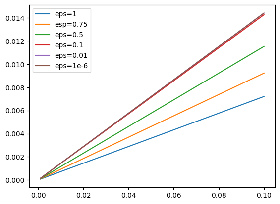
Figure 1:

We can see that the error is of the order of $h$ uniformly in $\epsilon$, for this particular example, that is due to the high regularity of $f$ and $A$.

References

- [1] J. Sin. Efficient Asymptotic-Preserving (AP) Schemes For Some Multiscale Kinetic Equations. SIAM Jour. Scient. Comp. 1999, 21 (2), 441-454
- [2] E. O’Riordan, M. Stynes. A globally uniformly convergent finite element method for a singularly perturbed elliptic problem in two dimensions. Math. of comp. (1991), 57-195: 47-62.
- [3] A.H. Schatz, L.B. Wahlbin. On the finite element method for singularly perturbed reaction-diffusion problems in two and one dimensions. Math. of Comp. (1983), 40 :47-89.
- [4] J. Li, I.M. Navon. Uniformly convergent finite element methods for singularly perturbed elliptic boundary value problems I: Reaction-diffusion Type. Comp. and Math. with App. (1998), 35-3: 57-70.
- [5] J. Li. Uniform convergence of discontinuous finite element methods for singularly perturbed reaction-diffusion problems. Comp. and Math. with App. (2002), 44 1–2: 231-240,
- [6] R. Lin. “Discontinuous Galerkin least-squares finite element methods for singularly perturbed reaction-diffusion problems with discontinuous coefficients and boundary singularities. Num. Math. (2009), 112: 295-318.
- [7] M. Chipot. On some anisotropic singular perturbation problems. Asymptot. Anal. (2007) 55: 125-144.
- [8] D. Maltese, C. Ogabi. On some new results on anisotropic singular perturbations of second-order elliptic operators. Com. Pur. App. Anal. (2023), 22-2: 639-667.
- [9] C. Ogabi. interior convergence for some class of elliptic anisotropic singular perturbations problems, Comp. Var. Ellip. Equ.(2019), 64: 574-585.
- [10] J.L. Lions. Perturbations singulieres dans les problemes aux limites et en controle optimal. Springer, 1973.
- [11] D. Gilbarg, N.S. Trudinger. Elliptic partial differential equations of second order. Springer,1979. 224-2.
- [12] S. C. Brenner, L. R. Scott. The mathematical theory of finite element methods. Springer, 2008.