Finite Blocklength Regime Performance of Downlink Large Scale Networks
Abstract
Some emerging 5G and beyond use-cases impose stringent latency constraints, which necessitates a paradigm shift towards finite blocklength performance analysis. In contrast to Shannon capacity-achieving codes, the codeword length in the finite blocklength regime (FBR) is a critical design parameter that imposes an intricate tradeoff between delay, reliability, and information coding rate. In this context, this paper presents a novel mathematical analysis to characterize the performance of large-scale downlink networks using short codewords. Theoretical achievable rates, outage probability, and reliability expressions are derived using the finite blocklength coding theory in conjunction with stochastic geometry, and compared to the performance in the asymptotic regime (AR). Achievable rates under practical modulation schemes as well as multilevel polar coded modulation (MLPCM) are investigated. Numerical results provide theoretical performance benchmarks, highlight the potential of MLPCM in achieving close to optimal performance with short codewords, and confirm the discrepancy between the performance in the FBR and that predicted by analysis in the AR. Finally, the meta distribution of the coding rate is derived, providing the percentiles of users that achieve a predefined target rate in a network.
Index Terms:
Average Coding Rate, Finite Blocklength, Meta Distribution, Multilevel Polar-Coded Modulation, Stochastic Geometry.I Introduction
The proliferating applications and diverse use-cases of beyond 5G (B5G) networks enforce stringent key performance indicators that cannot be realized via conventional coding schemes [2]. For instance, mission critical applications require sub- latency that cannot be achieved with conventional long codes [3]. Moreover, many Internet of Things (IoT) devices have an extreme low-power consumption profile that cannot support the complexity and long transmission intervals of conventional long codes [4]. Consequently, there is a paradigm shift towards using short codes to comply with the stringent latency and power consumption constraints of the foreseen B5G networks.111In a network, there are four dominant delays: transmission delay, propagation delay, processing delay, and queuing delay. As the network becomes denser, the transmission delay can dominate the propagation delay which motivates using short codes. Such reduced code length comes at the expense of inevitable errors and lower information coding rates. The tolerance to the induced errors differs with the application, which can be lower than for ultra-reliable low-latency communications (URLLC) [5]. This motivates the study of the finite blocklength coding theory [6, 7], which characterizes the information coding rate as a function of the code length and frame error rate (FER). Therefore, for a context-aware short code design in B5G networks, it is of primary importance to extend finite blocklength coding theory to interference-prone scenarios that account for the intrinsic large-scale and dense deployments of future networks.
Performance of large-scale cellular networks is well investigated using the classical Shannon capacity [8, 9, 10, 11, 12, 13], defined as the maximum achievable rate such that the error probability vanishes as the code length increases [14]. Such idealistic scenario is hereafter denoted as the asymptotic regime (AR). The AR analysis in [8, 9, 10, 11, 12, 13] is not applicable for networks operating in the finite blocklength regime (FBR). Short codes (e.g., 128 symbols) violate the AR assumptions and lead to inevitable errors as a cost for constraints on delay and/or power consumption. Thus, the code length of the FBR is a critical design parameter that imposes a delicate trade-off between FER () and information coding rate. To characterize such trade-off, the work of Polyanskiy et al. in [6, 7] finds the maximum achievable rate as function of the code length and FER for a point-to-point link.
Motivated by the need to migrate towards the FBR, the work in [6, 7] is extended for several use cases in [15, 16, 17, 18, 19, 20, 21, 22, 23, 24, 25]. For instance, the work in [15] extends the FBR analysis to relaying channels. The achievable rate for non-orthogonal multiple access in the FBR is studied in [16]. The impact of the FBR on rate splitting is characterized in [17]. The performance of multi-user MIMO, massive-MIMO, and cell-free MIMO in the FBR are investigated in [18], [19], and [20], respectively. The authors in [21, 22] optimize the blocklength and other network parameters (e.g., transmit power or transmitter location) to minimize the decoding error probability subject to a latency constraint. Works was also done in [23, 24, 25] to maximize the achievable rate, improve latency, enhance reliability, and/or provide a secure communication in the FBR. However, the models in [15, 16, 17, 18, 19, 20, 21, 22, 23, 24, 25] are limited to small scale networks. To the best of the authors’ knowledge, performance characterization of large-scale networks in the FBR is still an open problem.
Using the coding theory in the FBR in conjunction with stochastic geometry tools, this paper intends to contribute to the aforementioned research gap, as an extension of [1]. In particular, this paper develops novel mathematical analysis to characterize the trade-off between the code length , the FER , and the information coding rate in large-scale downlink (DL) networks using orthogonal multiple access (OMA). To this end, achievable rates and outage in the FBR are characterized for Gaussian codebooks as well as practical modulation schemes. Multi-level polar-coded modulation (MLPCM) [26, 27, 28, 29], is presented as a practical validation for the obtained theoretical achievable rates.222Polar codes is standardized for 5G in 3GPP Release 16 Specification 38.212[30], and MLPCM was proposed to be used in the future generations in [31, 32] The contributions of this paper are summarized as follows.
The paper analyzes the performance of a large-scale DL network in the FBR as a function of and in terms of:
-
•
the average coding rate under a random distance between the user and its serving BS, under Gaussian codebooks,
-
•
the average coding rate using QAM constellations,
-
•
the rate outage probability and reliability bounds and approximations, and
-
•
the approximation of the coding rate meta distribution.
Additionally, the paper simulates the average coding rate achieved by MLPCM for different QAM modulation orders in comparison with the obtained theoretical benchmarks. All results are validated via Monte Carlo simulations. It is shown that MLPCM achieves rates close to the derived theoretical benchmarks. It is also shown that the derived outage probability bounds are tight and coincide with simulation results. Additionally, it is shown that the proposed approximation of the coding rate meta-distribution is fairly tight under moderate and high SINR. Throughout the paper, we conduct qualitative and quantitative comparisons with the performance in the AR to motivate the importance of analyzing the performance in the FBR and demonstrate the discrepancy with AR results. We also investigate the effect of various network parameters in the FBR.
This paper is organized as follows. In Sec. II, the system model and assumptions of the analysis are presented. In Sec. III, the average coding rate of a large-scale DL network in the FBR is derived, under Gaussian codebooks and under a constraint of QAM constellations. Then, the theoretical results are numerically evaluated and compared with the performance of MLPCM as a practical scheme. In Sec. IV, bounds on the rate outage probability are derived, followed by the characterization of the reliability, the meta distribution of the coding rate, numerical evaluations, and a detailed discussion. Finally, the paper is concluded in Sec. V.
II System Model
Consider a single-tier OMA large-scale DL network with universal frequency reuse and no intra-cell interference. The base stations (BSs) are located according to a Poisson point process (PPP) with intensity . The network applies universal frequency reuse with one user equipment (UE) served per BS at a given resource block. Each UE is served by its geographically closest BS, where the intended distance between a UE and its serving BS is denoted as . The distances to the interfering BSs ordered with respect to the intended UE are denoted as such that . For the sake of simple presentation, the set is defined as the BSs distances to the desired UE. Hence, the received signal at the desired UE is given by
| (1) |
where is the transmit power of the BSs, (resp. ) represents the channel fading of the intended (resp. interfering) channel, is the path loss exponent, (resp. ) is a unit average power codeword symbol transmitted by the serving (resp. interfering) BS, is the aggregate interference from all other BSs, and is circularly symmetric complex Gaussian noise with zero mean and variance . We model and to be circularly symmetric complex Gaussian with zero mean and unit variance (modeling Rayleigh fading). An independent and identically distributed block fading channel model is assumed where the channel coefficients and remain constant for a duration of consecutive symbols and change to independent realizations at the end of each symbol interval.
The serving BS wants to send information to the UE using codewords from a code with the rate and length symbols, where can be defined following a latency and/or energy consumption constraint. To ensure that the channel remains constant during the transmission of symbols, we require for some integer [33]. This ensures that the channels remain constant during the transmission, but makes consecutive transmission blocks have identical channels. Nonetheless, by considering the sequence of blocks consisting of the first block (of symbols) in each coherence interval (of symbols), we have independent channels and we can derive the average performance over all transmissions. This is because the remaining sequences of blocks (such as the second frame in each coherence interval) have identical statistics.
To this end, two modes of operation are considered. The first mode assumes knowledge of channel-state information (CSI) at the transmitter and the receiver in the form of SINR availability.333Assuming SINR knowledge benchmarks the performance of the network. Under this mode, we investigate the average coding rate as a function of the FER and codelength (see Sec. III). The second mode assumes that the CSI is unknown at the transmitter but known at the receiver. Under this scenario, we derive the outage probability and utilize the coding-rate meta distribution to characterize the percentile of users achieving a given transmission reliability (See Sec. IV).
III Average Rate Analysis
Considering the first mode of operation, we assume that the SINR is available at the transmitter and the receiver. Hence, the coding rate can be adapted based on the SINR in each transmission block so that the transmission using codelength is successful with a desired FER . This rate adaptation can be realized using the following lemma, which characterizes the maximum achievable rate over an additive white Gaussian noise (AWGN) channel in the FBR [6].
Lemma 1.
([6]) For an AWGN channel with signal to noise power ratio (SNR) , blocklength , and FER , the maximum coding rate is approximated as444This approximation is shown to be tight at blocklengths () and FER in [6].
| (2) |
where is the AWGN channel capacity in the AR, is known as the channel dispersion, and is the inverse of the Q-function.
In this mode, due to the random changes of the channels and , we characterize performance by the average coding rate subject to a target FER and codelength . However, Lemma 1 is derived for an AWGN channel, and hence, cannot be directly applied to a large-scale network due to the additional non-Gaussian interference term in (1). To overcome this, we utilize the equivalence in distribution (EiD) approach to express the interference as a conditionally Gaussian random variable [34, 35, 12], as described next.
III-A Conditional Gaussian Representation
Using the EiD approach, we represent the aggregate interference for a given as follows
| (3) |
where denotes the EiD, and is a positive random variable independent of with a probability density function (PDF) whose Laplace transform (LT) is given by [12],
| (4) |
where is the transmitted symbol from an arbitrary codebook by an arbitrary BS and follows the same distribution as and .
The EiD in (3) is proved by showing that the product has the same characteristic function as [12]. Using (3), the equivalent system model is expressed as
where for a given , the lumped term is Gaussian with zero mean and variance . Hence, the resulting conditional SINR, given and , is given by
| (5) |
The random variable in (5) augments the noise power with the aggregate network interference power, for any constellation of and . If and is Gaussian distributed (Gaussian codebooks), it can be shown that (4) simplifies to [12]
| (6) |
Since at this point, interference is modeled as conditionally Gaussian, and since Lemma 1 provides a tight approximation when noise is Gaussian, then the tightness of the approximation provided in Lemma 1 holds here too. Thus, from this point onward, we focus on analyzing performance using as a surrogate for the maximum achievable rate in the FBR given that this is a tight approximation. Under this framework, the maximum average coding rate is defined next.
Definition 1.
Given a DL large-scale network with a distance between the desired UE and the serving BS as defined in (1), assuming the SINR knowledge is available at the transmitter and the receiver, we define the maximum average coding rate in the FBR with blocklength and FER with , as , where is the SINR defined in (5) and is as defined in Lemma 1.
III-B Average Coding Rate in the Finite Block-Length Regime
By virtue of the EiD, the AWGN results in Lemma 1 can be now extended to large-scale networks. For a given intended UE distance , the FBR average coding rate is characterized in the following theorem.
Theorem 1.
Proof.
By virtue of the EiD approach, Lemma 1 is applicable to large-scale networks by replacing by where is defined in (2), which leads to a maximum coding rate under a given and . The average rate is then , where the averaging is over and . Thus, we need to average and over and . The term is the average capacity in a large-scale network in the AR with CSI available at the BSs, which was derived in [36]. It remains to find which is shown to be equal to in App. A. ∎
Theorem 1 governs the maximum average rate at a fixed distance between the UE and its serving BS, considering the stochastic locations of the interfering BSs and the Rayleigh fading environment. The following corollary generalizes Theorem 1 by accounting for the randomness of .
Corollary 1.
The average coding rate of the large-scale network modeled by (1) with blocklength , FER , and Gaussian codebooks is given by
where and .
Proof.
As can be seen in Theorem 1 and Corollary 1, the average coding rate of the large-scale network in the FBR is the average capacity in the AR, plus a penalty term (loss) which is a function of the blocklength , and FER , in addition to the average SNR and the stochastic geometry of the network, manifested in the Laplace transform term. This penalty term implies a trade-off between the reliability and the average rate: the higher the reliability requirement (low FER), the lower the rate. However, for a given average achievable rate, the reliability can be increased ( decreased) by increasing the blocklength, converging to the AR performance as grows to infinity.
Theorem 1 expresses the average coding rate under Gaussian codebooks, which is of theoretical relevance. Characterizing the performance in the FBR when using a finite constellation is of practical interest and is discussed next.
III-C Average Rate Using Finite Constellations
This section focuses on achievable rates in the FRB under transmission using standard finite constellations. The maximum achievable rate using an -ary constellation over an AWGN channel in the FBR was given in [37]. Following the same methodology as in Sec. III-B, we use the EiD approach to extend the results of [37] to large-scale networks.
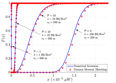
Consider an encoder that maps messages from a message set into a length sequence of symbols chosen from an -ary constellation consisting of complex-valued symbols . Using an -ary QAM constellation, denote by the average capacity achieved in the AR, by the average square root channel dispersion, and by the average coding rate under a blocklength and FER . To characterize the average capacity of the -ary QAM under FBR, the conditional mutual information has to be averaged with respect to the aggregate interference power and the channel gain . However, the distribution of the aggregate interference power is unknown which leads to an intractable expression. Although such an expression can be evaluated using Monte Carlo simulations, an expression that is amenable to numerical integration is preferable. A similar argument applies for . Hence, to obtain tractable integral expressions, we adopt an approximation for the distribution of the interference power proposed in [38, 39] which was shown to be a tight approximation. In particular, in [38, 39], the distribution of the interference power was approximated by a Gamma distribution
| (9) |
where is the shape parameter, and is the scale parameter. The approximation is based on a moment-matching approach. The first two moments of can be obtained from (4) as
The scale and shape parameters of the gamma distribution are then obtained as and , where .
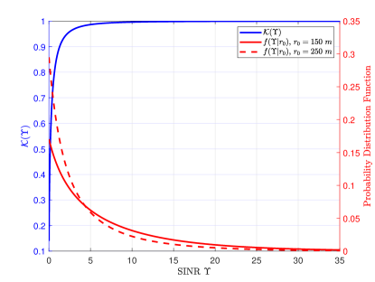
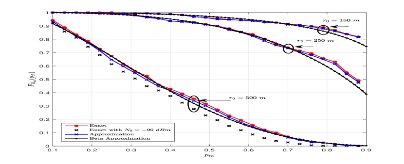
Fig. 1 numerically demonstrates the accuracy of this approximation by plotting the approximate CDF of (using (9)) and its exact CDF obtained from a numerical inversion of (4). The figure shows that the Gamma approximation in (9) provides a fairly tight approximation for the CDF of . Note that the Gamma approximation is crucial to maintain the tractability of the analysis. Using this approximation, the average coding rate of a large-scale network in the FBR, at a given distance and using -ary QAM constellation, is characterized.
The maximum achievable rate for a finite constellation is provided in [37]. However, the channel dispersion in [37] is defined as the variance of the information density (). This definition is considered to be imprecise according to [6], where the channel dispersion is defined as the conditional variance of the information density for finite constellation and is defined as the unconditional variance of the information density in the case of using Gaussian signals. Therefore, in this paper, we derive the maximum achievable rate using this definition for large-scale networks in the FBR in the following theorem.
Theorem 2.
For a DL large-scale network with BS density , blocklength , FER , distance between the UE and the serving BS, and an -ary constellation with symbols where and and are the real and imaginary parts of , respectively, if the interference power follows a Gamma distribution (9), then the average achievable coding rate can be expressed by
| (10) |
where ,
| (11) | ||||
| (12) | ||||
| (13) |
where , is a 2-D real-valued vector, is the SINR given in (5), and
| (14) |
Proof.
The average capacity of an -ary constellation () at a fixed is derived by averaging the conditional mutual information between the transmitted symbol and the received signal , i.e., , provided in [37], with respect to the SINR which is a function of interference power and fading channel statistics. Similarly, the average square-root channel dispersion () is derived by averaging the channel dispersion in (13) with respect to . The derivation of (13) is provided in App. B. However, instead of averaging over the distribution of which is unknown, we average over in (14) which is obtained using the Gamma approximation provided in (9) (See App. C). ∎
The following corollary generalizes Theorem 2 by accounting for the randomness of .
Corollary 2.
Proof.
This is derived by averaging (10) with respect to . ∎
The average achievable rate depends on the distances between symbols in the constellation set, i.e. for , where neighboring symbols contribute more to error than far ones. Such distances are in turn affected by the constellation choice. Moreover, the average achievable rate is affected by the network parameters which will be investigated later in the numerical evaluations section.
III-D Multilevel Polar-Coded Modulation
To validate the theoretical results in Sec. III-B and III-C, we use the MLPCM scheme shown in Fig. 2. The information bits (message) are fed into a demultiplexer that splits them into sub-messages where . Each sub-message is encoded using a polar encoder with rate to obtain codewords , where is the row of ( codeword). Then, the transmitter collects one bit from each of the codewords to form a -bit symbol which is then mapped to a symbol from an -ary constellation such as the -QAM constellation. The symbols are then scaled according to the power constraint in Sec. II. The result of repeating this process for all codeword symbols of all sub-messages is one MLPCM codeword of length , which is then transmitted through the channel. At the receiver side, multistage decoding takes place to efficiently recover the message. It breaks the decoding process into stages.
In each stage , the receiver feeds the demapper of the stage with the received signal and the submessages recovered from previous stages , (which is defined as for ), and the demapper demaps the symbols into bits to obtain , using the multilevel decoding criteria [26]. Then, the demapped bits are decoded using a polar decoder to obtain using the successive cancellation algorithm provided in [40]. Finally, all sub-messages are fed to a multiplexer to form the message . This MLPCM will be incorporated in the large-scale DL network Monte Carlo simulator to validate the achievability of the theoretical rates obtained in Sec. III-B and III-C.

III-E Average Rate Numerical Results
This subsection presents illustrative numerical results for the theoretical rate analysis provided in Sec. III-B and III-C, which are also validated via Monte Carlo simulation. The results presented investigate the effect of the blocklength and the FER , the tightness of the proposed theoretical approximations, and the performance comparison between the FBR and the AR. Then, the performance of the MLPCM is investigated in comparison with the theoretical average coding rate.
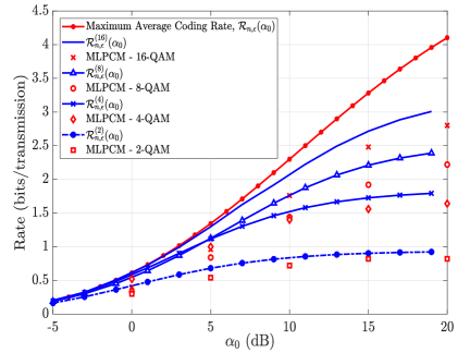
Fig. 3 plots the maximum average coding rate and the average coding rate for M-QAM versus the average SNR for a fixed . In Fig. 3(a), the average coding rate is plotted for , FER , and m. Given a FER , a gap exists between the average coding rate in the FBR and the AR. The gap is around dB for and is between and dB for at and , respectively, which shows the severity of the SNR penalty in the FBR compared to the AR. The figure shows the trade-off between reliability (represented by FER) and maximum average coding rate at a given , where the maximum average coding rate decreases/increases as the FER decreases/increases. For instance, to achieve a given maximum average coding rate at and FER , we need around dB more power compared with the same blocklength under the FER . Furthermore, the impact of small becomes more severe when the FER is smaller, resulting in rate degradation. Overall, this shows that it is impractical to use results from the AR in the FBR.
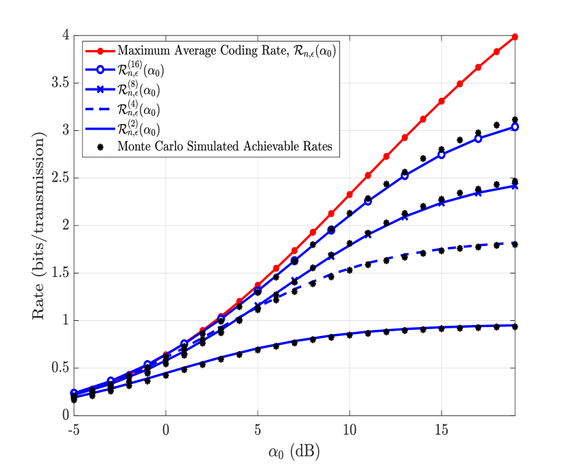
Second, the maximum achievable coding rate for different modulation schemes, presented in Sec. III-C, is simulated for , , blocklength , and FER in Fig. 3(b). Fig. 3(b) demonstrates the approximated maximum achievable coding rate using the Gamma approximation for various modulation orders, , (Theorem 2), along with the maximum achievable rate under Gaussian codebooks (Theorem 1) versus . The Monte Carlo simulated maximum achievable coding rate for QAM is provided to show the tightness of the approximation. The approximated maximum achievable rate is very close to the simulated maximum achievable rate. Thus, the Gamma approximation in (9) leads to a fairly tight approximation. It is also observed that as the QAM modulation order increases, the performance improves towards the maximum average coding rate (without Gaussian codebooks) in a large-scale network in the FBR (Theorem 1).
The spatially averaged coding rate is depicted in Fig 4(a) versus the transmit signal to noise power ratio .555The figure is plotted for a wide range of for illustrative purposes, bearing in mind that some values of in the plot may be impractical. The figure shows that for high SNR (above dB), one cannot achieve the same rate and FER achieved at a given by decreasing and paying an SNR penalty. For instance, the rate achieved at , , dB cannot be achieved at and . The only way to achieve such a rate at is by paying a FER penalty, which is impractical for applications that need high reliability. Hence, it is important to select that balances the trade-off between reliability and coding rate. Similar to Fig. 3(a), Fig. 4(a) shows the importance of the results in this paper for characterizing and optimizing the performance of large-scale networks with latency-sensitive applications.
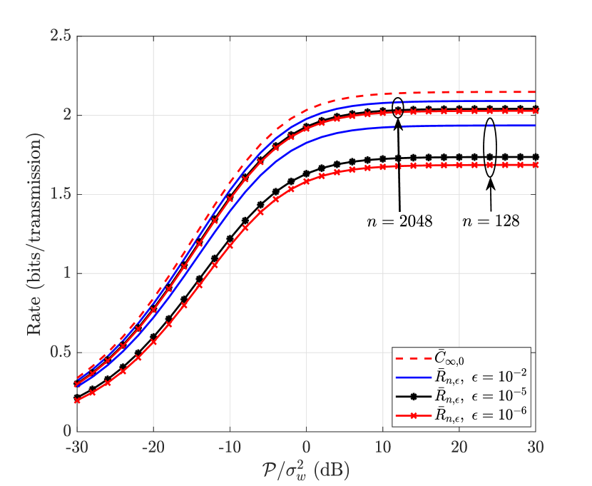
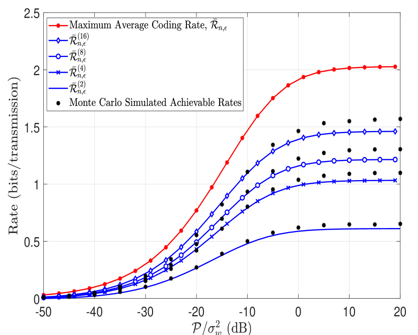
Fig. 4(b) plots, the average achievable rate versus under a Rayleigh distributed , QAM constellation with and , blocklenth , and FER , showing a similar trend as for fixed . It is observed that the average achievable rate saturates at a rate of for this choice of , , and , which is low compared to the case . This performance is a consequence of averaging the performance of nearby UEs which have relatively strong received desired signals (high SINR) and far away UEs which suffer from more interference (low SINR).
Finally, considering the same setting in Fig. 3(b), we simulate MLPCM with a QAM constellation for modulation orders and in Fig. 5. The simulations are performed by fixing the SNR and increasing the coding rate until reaching the FER . The achievable rates are plotted along with the theoretical expressions proposed in (7) and (10). The figure shows that the achievable rates of the MLPCM scheme with 2-QAM or 4-QAM approaches the theoretical rate of the corresponding QAM constellation. However, for 8-QAM and 16-QAM, a gap of dB exists between the theoretical results and the simulation results. Nonetheless, this SNR gap translates to a small rate gap of fractions of bits/transmission due to the slow increase of the rate versus SNR in the large-scale network which is caused by interference. Fig. 5 thus validates that the theoretical performance under finite constellations can be approached using MLPCM, which validates the potential of MLPCM for future technologies.
IV Rate Outage Probability & Meta Distribution
In the previous section, we studied the case where the SINR is known at the transmitter. However, if the BS does not track the SINR, then the rate adaptation investigated in the previous section is not possible. Considering the second mode of operation, where the SINR is unknown at the transmitter but known at the receiver, the transmitter encodes at a constant (target) rate and blocklength . As a result, the resulting (conditional) FER conditioned on SINR may or may not satisfy a desired design FER due to the unknown stochastic variation of the intended channel fading and aggregate interference. In this case, it is important to keep this conditional FER below a threshold. This is especially relevant bearing in mind that , i.e., a large conditional FER means that there are coherence intervals that produce large FERs for all blocks within these coherence intervals. This can lead to bursts of frame errors when the channel undergoes a period of coherence intervals with weak channels, which is undesired.
Thus, we define an FER threshold , and it is desired to maintain the conditional FER below . If the conditional FER exceeds , we say that we have an outage. This equivalently means that rate supported by the channel at the given and FER threshold decreases below . This is defined formally as follows.
Definition 2.
Given a target rate and a DL large-scale network with a distance between the desired UE and the serving BS as defined in (1), we define the outage probability in the FBR with blocklength and FER threshold as , where is as defined in Lemma 1.
This outage probability is studied in this section.
IV-A DL Outage Analysis in the Finite Blocklength Regime
We start by reviewing the outage probability of a large-scale network in the AR. In this case, the outage is defined as the probability that the channel capacity (defined as the maximum rate such that the error probability vanishes as ) is lower than a target rate . The rate outage probability under a given is given as [41]
| (16) |
Studying the rate outage probability under blocklength and FER threshold is generally difficult to simplify as it is a function of the fading distribution as well as the network geometry. Instead, we provide bounds which are fairly tight in the following theorem.
Theorem 3.
Proof.
The outage probability lower bound confirms that the outage probability in the FBR is larger than that in the AR and the upper bound provides a guaranteed performance. By observing Fig. 6, it can be seen that quickly approaches one as grows. The figure also shows that the density in the interval of SINR, where the approximation is tight ( e.g. ), increases as decreases (which is the case for dense networks). Hence, the upper bound can be used to evaluate guaranteed outage performance in general and can be used as a tight approximation for dense networks. This is verified in Fig. 7 & 8. Next, the spatially averaged outage probability is presented.
Corollary 3.
The average rate outage probability defined in Def. 2 with blocklength , FER , and target rate can be upper bounded as
| (20) |
Proof.
Using the law of iterated expectation, the average outage probability is the average of (18) with respect to , i.e., . The result then follows since follows a Rayleigh distribution. ∎
For a shadowed urban cellular network, the path-loss exponent lies in the range [42], where is a common value of practical relevance that is widely utilized in the literature. For the case , the outage probability in (20) can be simplified as given next.
Corollary 4.
The average rate outage probability of the large-scale network modeled by (1) with blocklength , FER , target rate , and path loss exponent , can be upper bounded as
| (21) |
where and .
Proof:
A closed-form expression for the upper bounded outage probability at is obtained as follows
| (22) | ||||
| (23) | ||||
| (24) |
where we used , is obtained using a change of variable , and is obtained using the change of variables and the CDF of the Gaussian distribution with mean and variance . ∎
The rate outage probability of a large-scale network in the FBR is upper bounded, with guaranteed performance at high SINR, in a generic form in (18) and (20) and in a closed-form expression for in (24), as a function of BS density , FER , blocklength , and average SNR . Next, the reliability of the network under the FBR.
IV-B Reliability of a Large-Scale Network in the Finite Blocklength Regime
We define a metric to evaluate the overall network reliability for a fixed , defined as the probability of correctly decoding a codeword. A codeword is decoded correctly in two cases in the FBR. The first case is when , in which case the codeword is decoded correctly with a probability larger than or equal to . The second case is when , in which case few codewords may still be decoded correctly. Since in practice, it is desirable to operate at low outage probability, hence the second case does not contribute much to reliability. Thus, to simplify the analysis, we will lower bound the probability of decoding a codeword correctly in the second case by (i.e., its contribution to reliability is neglected) and we will only consider the first case. Hence, the reliability is lower bounded by the following expression, providing a guaranteed performance for a given ,
| (25) |
The guaranteed reliability averaged over is given by
| (26) |
Also, for the sake of comparison, the reliability of the AR can be defined as
| (27) |
since the error probability is assumed to be vanishing as , and hence failure occurs when there is an outage. The reliability will be assessed numerically in Sec. IV-D.
Studying the rate outage probability and the overall system reliability gives more insight into the performance of the network. Moreover, studying the coding rate meta distribution, which provides the percentiles of users achieving a rate , will provide a complete picture of the network performance. Hence, the meta distribution of the coding rate is derived next.
IV-C Coding Rate Meta Distribution in the Finite Blocklength Regime
The meta distribution provides fine-grained information about network performance, in the form of the fraction of users that can achieve a minimum data rate at a FER threshold with probability at least . The definition and analysis of this quantity are provided next.
Definition 3.
Given a target rate and a DL large-scale network with a distance between the desired UE and the serving BS as defined in (1), we define the coding rate meta distribution in the FBR with blocklength and FER threshold as where is the probability of success, is the signal-to-interference ratio (SIR) and is as defined in Lemma 1.
For simplicity, we assume an interference-limited scenario where noise is neglected and the SIR is given by . Then, is given by
| (28) |
where is the reduced Palm measure of the point process [43],[44, Def. 8.8]. Note that is a random variable which is a function of the stochasticity of the network. Its moments are defined as
| (29) |
and are used to calculate the meta distribution as follows [43]
| (30) |
where is the imaginary part of a complex number and is obtained at in (29).
In [43], a simple yet tight approximating distribution of is proposed for the AR, which is the beta distribution given by
| (31) |
where is the beta function, and the . Hence, the meta distribution could be computed as the CCDF of the beta distribution. However, and provided in (29) are difficult to evaluate in the FBR, and hence, an approximation is proposed in this paper. At high SIR, where the term is approximately equal to 1, the approximated probability of success is given by
Therefore, the approximated probability of success can be expressed as a function of the SIR instead of the coding rate, as follows,
| (32) |
The expression provided in (32) is obtained by averaging over the channel gains. Then, its moments are given by
| (33) |
Thus, the meta distribution can be evaluated using the approximated moments in (IV-C) as follows
| (34) |
Using the beta distribution approximation, the meta-distribution can be approximated as
| (35) |
where is the regularized incomplete beta function.
IV-D Numerical Results
Now, we provide numerical results for the bounds and approximations of the rate outage probability, reliability, and the coding rate meta-distribution. We investigate the tightness of these approximations and compare them with results from the literature for the AR.
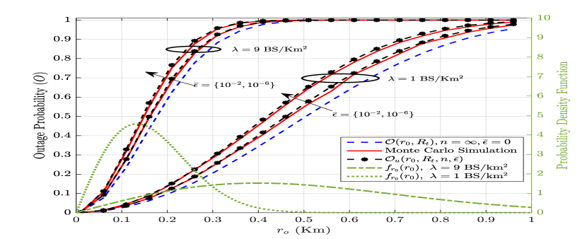
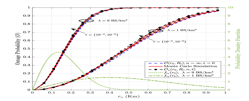
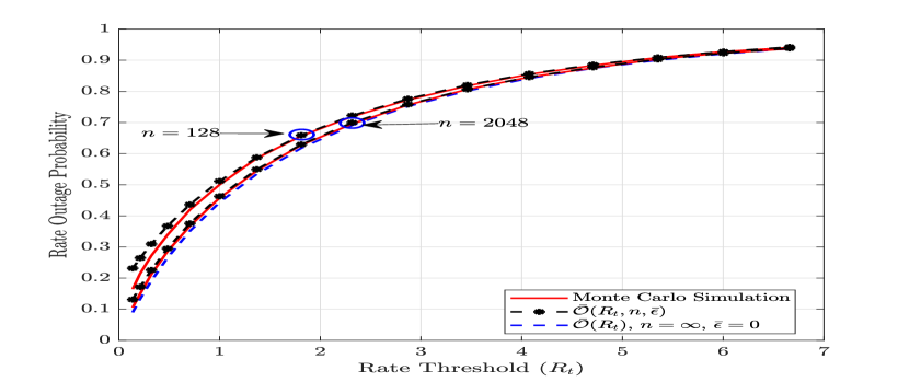
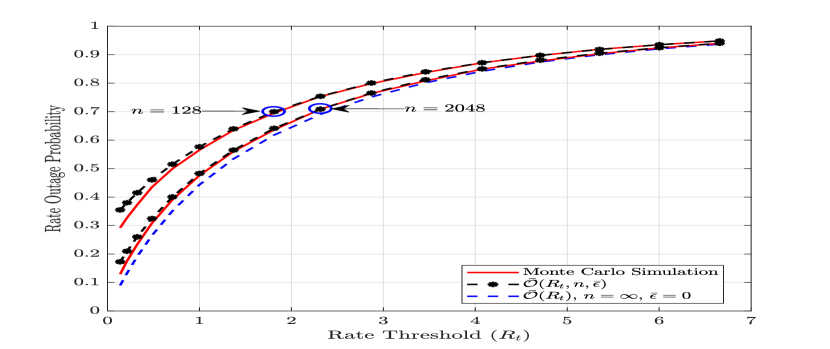
First, in Fig. 7, the rate outage probability is plotted versus with , , , , and bit/transmission. The PDF of is plotted to illustrate the probability of occurrence of the values. The figure shows the Monte Carlo simulated outage probability, in addition to the upper bound in (18) and the outage probability in the AR (16) which serves as a lower bound (cf. Thm. 3). It shows that the rate outage in the AR underestimates the rate outage probability in the FBR and the gap to the actual outage probability increases as the FER threshold decreases. This gap can be as large as in some cases, such as with m, BS/km2, , and , where the actual outage probability is 0.13, but (16) underestimates it as 0.1. Fig. 7 also shows that the upper bound of the outage probability expression in (18) is fairly accurate to provide a convenient approximation for a broad range of , and . The outage probability is seen to increase as the FER threshold decreases because the term in (7) increases as decreases. However, at a specific , as increases, the outage probability approaches the outage probability in the AR as expected. Thus, while the results in [12] can be a good representative of the performance when is relatively large (Fig. 7(a)), this is not the case when is small in which case our derived bounds and approximation are more accurate. Moreover, in Fig. 8, the rate outage probability approximation for a Rayleigh distributed , provided in (24), is plotted versus the target rate and compared to the simulated outage probability for BS density , blocklengths , FER threshold , and . This plot also proves the tightness of the upper bound and the inaccuracy of the AR.
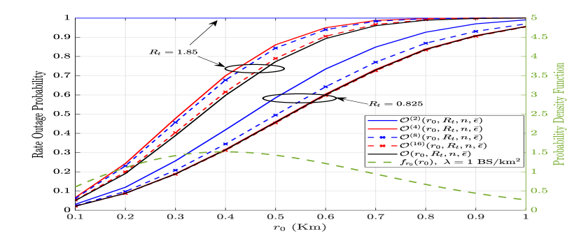
In Fig. 9(a), the rate outage probability under QAM constellations is shown for various modulation orders versus , where the rate outage for a specific modulation scheme is defined as . This expression is computed using Monte Carlo simulation. The figure is plotted for , , , , and . Similar to the previous plots, the rate outage probability acts as the lower bound of the outage probability of all constellation sets. Also, the higher order modulation (i.e. ) yields an outage probability lower than the lower order modulation (i.e. ) at a fixed as the modulation order limits the maximum transmission rate . However, at lower as such , most of the high order modulation schemes provide a performance close to the theoretical lower bound . Fig. 9(b) shows the outage probability for random , i.e., versus . As shown, the rate outage probability increases as the rate threshold increases, and it jumps to 1 at a certain for each modulation order, which is when exceeds the maximum rate achievable by the modulation order ().

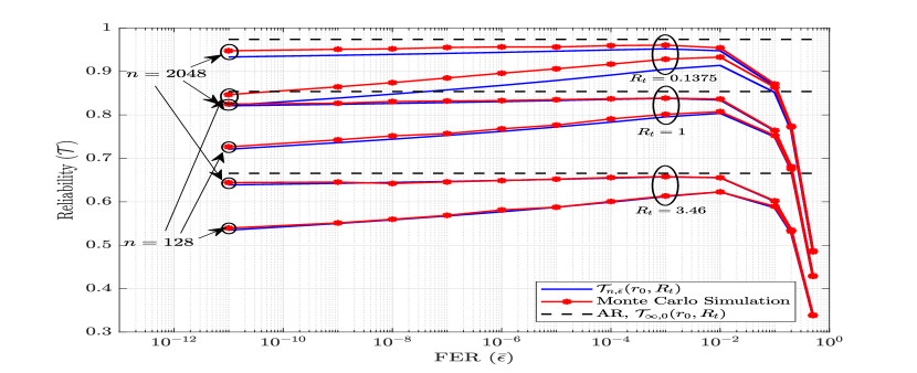
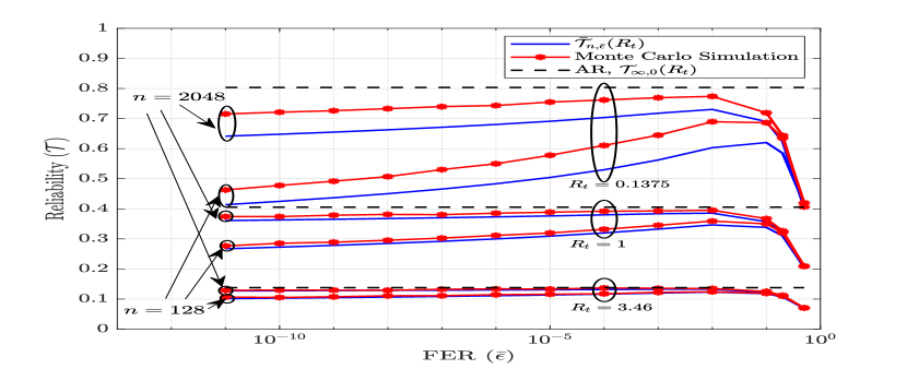
The overall network reliability versus the FER threshold is evaluated in Fig. 10 for fixed and random for and . It can be observed that the reliability of the network increases as the FER threshold increases until it reaches a maximum around then it rapidly decays. This is because the increase of with respect to is faster than the decrease of for small . However, for large , saturates to and dominates and contributes to the decay of the reliability at high . In other words, at , the rate of increase of is higher than the rate of decay of . However, at , the rate of increase of is nearly zero and the rate of decay of dominates. Therefore, the reliability rapidly decays. It is shown that for a fixed , a gap exists between curves simulated under FBR and AR. This gap grows wider up to as FER threshold decreases because the short blocklengths (e.g. ) are less reliable. Also, it is obvious that the reliability of the network at random is lower than that at fixed as it averages the performance of users which are close and those that are far away from the BS. Moreover, as increases the approximated reliability becomes close to the exact one. This is because the outage upper bound provided in Corollary 3 is tight for high SINR. Hence, from Def. 2, as the increases, only high SINRs can achieve the desired rate and FER threshold at the given , which is where the approximation becomes tighter. Whereas, for low , low SINRs can also achieve the desired performance which loosens the approximation.
Finally, we validate the coding rate meta distribution in Fig. 11(a). The coding rate meta distribution provided in (30) is simulated via Monte-Carlo simulations at , , an area of , a blocklength , FER threshold , and a rate threshold . It is observed that there is a significant gap between the performance in the AR and the FBR, showing that the meta distribution of the coding rate in the AR overestimates the performance of the network in the FBR. This gap can reach up to at and , which means of the users predicted to achieve the required performance in the AR will not achieve it in the FBR. It can also be observed that the gap increases as or increases. Thus, the AR analysis in [43, 45, 46] cannot be used to provide precise results in the FBR. For the sake of preciseness of the results, we have simulated the coding rate meta distribution including the noise term with noise power [47]. The results show that the network is an interference-limited network and the noise can be neglected for the simplicity of the analysis. In Fig. 11(b), the approximation proposed in (32) is shown to be very tight compared to the exact coding rate meta distribution in (30) for different . The tightness of the approximation increases by decreasing or alternatively increasing SIR as the term converges to as the SIR increases. Using this approximation it is easier to find an expression for the moments of the success probability and use it to evaluate the meta distribution using the beta distribution provided in (35). Hence, the beta approximation of the meta-distribution provides a close performance to the exact and approximated meta-distribution.

Thus, we saw that our proposed expressions provide an accurate representation of the rate outage probability and the coding rate meta distribution in the FBR, which is more accurate than using AR expressions from the literature.
V Conclusion
This paper investigates different aspects of the performance of a large-scale DL network in the FBR using the theory of coding in the FBR in conjunction with stochastic geometric tools. We start with rate analysis where we derive the average coding rate using Gaussian codebooks and -ary QAM constellation, and investigate the practical scheme of MLPCM in the FBR showing that its performance approaches the theoretical benchmarks. We also study the rate outage probability, reliability, and the coding rate meta distribution, where we provide bounds and approximations. From the results, we conclude that the performance analysis provided under an AR provides a misleading (overestimated) performance and cannot be used to characterize the performance in the FBR. The performance in the FBR provides accurate rate and FER characterization, and approaches the AR performance at sufficiently large blocklengths and high FER . The developed expressions for the average coding rate, the rate outage probability, and the coding rate meta distribution are fairly tight as shown by our numerical results. In conclusion, the results are relevant for the theoretical analysis of large-scale networks in the FBR, and the theoretical performance can be approached using practical transmission schemes such as MLPCM. The results in this paper can be extended to characterize the performance of networks under different multiple access schemes as in [48, 18, 17].
Appendix A The Average Square Root Channel Dispersion
From the definition of channel dispersion provided in (2), the average square root channel dispersion can be written as follows
| (36) |
where is the cumulative distribution function (CDF) of , and the last step follows as an application of Fubini’s theorem [49]. The CDF of for a given is given by
| (37) |
where the last step follows from the exponential distribution of . Averaging with respect to the interference term yields . Hence, the CDF of the square root of the channel dispersion is given as
| (38) |
which is obtained using the definition of Laplace transform . By substituting (38) in (36), we obtain
as defined in Theorem 1.
Appendix B The Channel Dispersion for A Large-Scale Network Under a Finite Constellation
The channel dispersion is defined as the conditional variance of the information density conditioned on the input distribution as follows
where is the 2-D real-valued vector form of the complex-valued symbol of an -ary constellation.
Define and . The first term is derived as follows
The term is given by
where . Define , hence by substitution, is given by
The term is given by
and is divided into four terms as , where
where follows from a change of variable , and follows by using and , and is given by
where is obtained by the substitution of , , and .
The term is given by
and is divided into three terms as , where
By adding , , and , is given by
The second term is the square of the relative entropy given as
To compute the average square-root channel dispersion, is subtracted from and then averaged over all constellation symbols, leading to the following expression as indicated in (13)
Appendix C The SINR distribution at a Fixed
References
- [1] N. Hesham and A. Chaaban, “On the performance of large-scale wireless networks in the finite block-length regime,” in ICC 2021 - IEEE Int. Conf. Commun., 2021, pp. 1–6.
- [2] Z. Ma, M. Xiao, Y. Xiao, Z. Pang, H. V. Poor, and B. Vucetic, “High-reliability and low-latency wireless communication for internet of things: Challenges, fundamentals, and enabling technologies,” IEEE Internet of Things Journal, vol. 6, no. 5, pp. 7946–7970, 2019.
- [3] H. Yu, H. Lee, and H. Jeon, “What is 5G? emerging 5G mobile services and network requirements,” Sustainability, vol. 9, no. 10, p. 1848, 2017.
- [4] A. J. Pinheiro, J. de M. Bezerra, C. A. Burgardt, and D. R. Campelo, “Identifying IoT devices and events based on packet length from encrypted traffic,” Comput. Commun., vol. 144, pp. 8 – 17, 2019.
- [5] W. Khalid, H. Yu, R. Ali, and R. Ullah, “Advanced physical-layer technologies for beyond 5G wireless communication networks,” Sensors, vol. 21, no. 9, 2021. [Online]. Available: https://www.mdpi.com/1424-8220/21/9/3197
- [6] Y. Polyanskiy, H. V. Poor, and S. Verdú, “Channel coding rate in the finite blocklength regime,” IEEE Trans. Inf. Theory, vol. 56, no. 5, pp. 2307–2359, 2010.
- [7] W. Yang, G. Durisi, T. Koch, and Y. Polyanskiy, “Block-fading channels at finite blocklength,” in Int. Symp. Wireless Commun. Sys., 2013, pp. 1–4.
- [8] H. Q. Nguyen, F. Baccelli, and D. Kofman, “A stochastic geometry analysis of dense IEEE 802.11 networks,” in IEEE Int. Conf. Comput. Commun., 2007, pp. 1199–1207.
- [9] M. Haenggi, J. G. Andrews, F. Baccelli, O. Dousse, and M. Franceschetti, “Stochastic geometry and random graphs for the analysis and design of wireless networks,” IEEE J. Sel. Areas Commun., vol. 27, no. 7, pp. 1029–1046, 2009.
- [10] C.-H. Lee, C.-Y. Shih, and Y.-S. Chen, “Stochastic geometry based models for modeling cellular networks in urban areas,” Wireless Netw., vol. 19, no. 6, pp. 1063–1072, 2013.
- [11] Y. Hmamouche, M. Benjillali, S. Saoudi, H. Yanikomeroglu, and M. D. Renzo, “New trends in stochastic geometry for wireless networks: A tutorial and survey,” Proc. IEEE, vol. 109, no. 7, pp. 1200–1252, 2021.
- [12] H. ElSawy, A. Sultan-Salem, M.-S. Alouini, and M. Z. Win, “Modeling and analysis of cellular networks using stochastic geometry: A tutorial,” IEEE Commun. Surveys Tuts., vol. 19, no. 1, pp. 167–203, 2016.
- [13] H. ElSawy, E. Hossain, and M. Haenggi, “Stochastic geometry for modeling, analysis, and design of multi-tier and cognitive cellular wireless networks: A survey,” IEEE Commun. Surveys Tuts., vol. 15, no. 3, pp. 996–1019, 2013.
- [14] C. E. Shannon, “Coding theorems for a discrete source with a fidelity criterion,” IRE Nat. Conv. Rec, vol. 4, no. 142-163, p. 1, 1959.
- [15] Y. Hu, J. Gross, and A. Schmeink, “On the capacity of relaying with finite blocklength,” IEEE Trans. Veh. Technol., vol. 65, no. 3, pp. 1790–1794, 2015.
- [16] E. Dosti, M. Shehab, H. Alves, and M. Latva-aho, “On the performance of non-orthogonal multiple access in the finite blocklength regime,” Ad Hoc Networks, vol. 84, pp. 148 – 157, 2019. [Online]. Available: http://www.sciencedirect.com/science/article/pii/S157087051830708X
- [17] Y. Xu, Y. Mao, O. Dizdar, and B. Clerckx, “Rate-splitting multiple access with finite blocklength for short-packet and low-latency downlink communications,” arXiv preprint arXiv:2105.06198, 2021.
- [18] J. Feng, H. Q. Ngo, and M. Matthaiou, “Coherent MU-MIMO in block fading channels: A finite blocklength analysis,” in IEEE Int. Conf. Commun. Workshops (ICC Workshops), 2020, pp. 1–6.
- [19] J. Östman, A. Lancho, G. Durisi, and L. Sanguinetti, “URLLC with massive MIMO: Analysis and design at finite blocklength,” IEEE Trans. Wireless Commun., vol. 20, no. 10, pp. 6387–6401, 2021.
- [20] A. Lancho, G. Durisi, and L. Sanguinetti, “Cell-free massive MIMO with short packets,” in IEEE Int. Workshop Signal Process. Adv. Wireless Commun. (SPAWC), 2021, pp. 416–420.
- [21] H. Ren, C. Pan, Y. Deng, M. Elkashlan, and A. Nallanathan, “Joint power and blocklength optimization for URLLC in a factory automation scenario,” IEEE Trans. Wireless Commun., vol. 19, no. 3, pp. 1786–1801, 2020.
- [22] W. J. Ryu and S. Y. Shin, “Power allocation for URLLC using finite blocklength regime in downlink NOMA systems,” in Int. Conf. Inf. Commun. Technol. Convergence (ICTC), 2019, pp. 770–773.
- [23] C. Shen, T.-H. Chang, H. Xu, and Y. Zhao, “Joint uplink and downlink transmission design for URLLC using finite blocklength codes,” in Int. Symp. Wireless Commun. Sys. (ISWCS), 2018, pp. 1–5.
- [24] Z. Wang, T. Lv, Z. Lin, J. Zeng, and P. T. Mathiopoulos, “Outage performance of URLLC NOMA systems with wireless power transfer,” IEEE Wireless Commun. Lett., vol. 9, no. 3, pp. 380–384, 2020.
- [25] H. Ren, C. Pan, Y. Deng, M. Elkashlan, and A. Nallanathan, “Resource allocation for secure URLLC in mission-critical IoT scenarios,” IEEE Trans. Commun., vol. 68, no. 9, pp. 5793–5807, 2020.
- [26] M. Seidl, A. Schenk, C. Stierstorfer, and J. B. Huber, “Polar-coded modulation,” IEEE Trans. Commun., vol. 61, no. 10, pp. 4108–4119, 2013.
- [27] H. Khoshnevis, I. Marsland, and H. Yanikomeroglu, “Throughput-based design for polar-coded modulation,” IEEE Trans. Commun., vol. 67, no. 3, pp. 1770–1782, 2019.
- [28] T. Koike-Akino, Y. Wang, D. S. Millar, K. Kojima, and K. Parsons, “Polar coding for multilevel shaped constellations,” in OSA Signal Process. Photonic Commun., 2018, p. SpW1G.1.
- [29] H. Khoshnevis, “Multilevel polar coded-modulation for wireless communications,” Ph.D. dissertation, Carleton University, 2018.
- [30] 3GPP, “Technical Specification Group Radio Access Network; NR; Multiplexing and channel coding,” 3rd Generation Partnership Project (3GPP), TS 38.212, Release 16, V16.8.0, Jan. 2022.
- [31] J. Dai, D. Zhang, K. Niu, Z. Si, P. Zhang, S. Wang, Y. Yuan et al., “Generalized polarization transform: A novel coded transmission paradigm,” arXiv preprint arXiv:2110.12224, 2021.
- [32] B. Tomasi, F. Gabry, V. Bioglio, I. Land, and J.-C. Belfiore, “Low-complexity receiver for multi-level polar coded modulation in non-orthogonal multiple access,” in 2017 IEEE Wireless Communications and Networking Conference Workshops (WCNCW), 2017, pp. 1–6.
- [33] E. Malkamaki and H. Leib, “Performance of truncated type-II hybrid ARQ schemes with noisy feedback over block fading channels,” IEEE Trans. Commun., vol. 48, no. 9, pp. 1477–1487, 2000.
- [34] M. D. Renzo and W. Lu, “The equivalent-in-distribution (EiD)-based approach: On the analysis of cellular networks using stochastic geometry,” IEEE Commun. Lett., vol. 18, no. 5, pp. 761–764, 2014.
- [35] P. C. Pinto and M. Z. Win, “Communication in a Poisson field of interferers–part I: Interference distribution and error probability,” IEEE Transactions on Wireless Communications, vol. 9, no. 7, pp. 2176–2186, 2010.
- [36] J. G. Andrews, F. Baccelli, and R. K. Ganti, “A tractable approach to coverage and rate in cellular networks,” IEEE Trans. Commun., vol. 59, no. 11, pp. 3122–3134, 2011.
- [37] C. Zhag, X. Mu, J. Yuan, Y. Zhou, and J. Shi, “The performance of coded modulation with Gallager mapping in the finite length regime,” in Int. Conf. Wireless Commun. Signal Process. (WCSP), 2019, pp. 1–6.
- [38] R. K. Ganti and M. Haenggi, “Interference in ad hoc networks with general motion-invariant node distributions,” in IEEE Int. Symp. Inf. Theory. IEEE, 2008, pp. 1–5.
- [39] M. Kountouris and N. Pappas, “Approximating the interference distribution in large wireless networks,” in Int. Symp. Wireless Commun. Sys. IEEE, 2014, pp. 80–84.
- [40] H. Vangala, E. Viterbo, and Y. Hong, “Permuted successive cancellation decoder for polar codes,” in Int. Symp. Inf. Theory Appl., 2014, pp. 438–442.
- [41] J. G. Andrews, A. K. Gupta, and H. S. Dhillon, “A primer on cellular network analysis using stochastic geometry,” arXiv preprint arXiv:1604.03183, 2016.
- [42] F. Palacio, R. Agustí, J. Pérez-Romero, M. López-Benítez, S. Grimoud, B. Sayrac, I. Dagres, A. Polydoros, J. Riihijärvi, J. Nasreddine, P. Mähönen, L. Gavrilovska, V. Atanasovski, and J. Beek, “Radio environmental maps: information models and reference model. document number D4.1,” Deliverable D4.1 del projecte Europeu FARAMIR (248351), 2011.
- [43] M. Haenggi, “The meta distribution of the SIR in Poisson bipolar and cellular networks,” IEEE Trans. Wireless Commun., vol. 15, no. 4, pp. 2577–2589, 2016.
- [44] ——, Stochastic Geometry for Wireless Networks. Cambridge University Press, 2012.
- [45] H. ElSawy and M.-S. Alouini, “On the meta distribution of coverage probability in uplink cellular networks,” IEEE Commun. Lett., vol. 21, no. 7, pp. 1625–1628, 2017.
- [46] H. Ibrahim, H. Tabassum, and U. T. Nguyen, “The meta distributions of the SIR/SNR and data rate in coexisting sub-6GHz and millimeter-wave cellular networks,” IEEE Open J. Commun. Soc., vol. 1, pp. 1213–1229, 2020.
- [47] W. Hassan, H.-S. Jo, S. Ikki, and M. Nekovee, “Spectrum-sharing method for co-existence between 5G OFDM-based system and fixed service,” IEEE Access, vol. 7, pp. 77 460–77 475, 01 2019.
- [48] K. S. Ali, M. Haenggi, H. ElSawy, A. Chaaban, and M.-S. Alouini, “Downlink non-orthogonal multiple access (NOMA) in Poisson networks,” IEEE Trans. Commun., vol. 67, no. 2, pp. 1613–1628, 2018.
- [49] G. Fubini, “Sugli integrali multipli,” Rend. Acc. Naz. Lincei, vol. 16, pp. 608–614, 1907.