Chain recurrence and Selgrade’s theorem for affine flows

Fritz Colonius${}^{1^{*}}$     and     Alexandre J. Santana2†
1Institut fü Mathematik, Universität Augsburg, Universitätsstraße 2,
Augsburg, 86159, Germany.
2Department of Mathematics, State University of Maringa,
Av. Colombo, 5790, Maringa, 87020-900, Brazil.
Corresponding author. E-mail: fritz.colonius@uni-a.de;
Contributing author: ajsantana@uem.br;
This author contributed equally to this work
Abstract

Affine flows on vector bundles with chain transitive base flow are lifted to linear flows and the decomposition into exponentially separated subbundles provided by Selgrade’s theorem is determined. The results are illustrated by an application to affine control systems with bounded control range.

Key words: affine flows, Selgrade’s theorem, chain transitivity, Poincaré sphere, affine control systems
MSC Classification: 37B20, 34H05, 93B05

1 Introduction

For linear (skew product) flows on vector bundles, Selgrade’s theorem describes the decomposition into subbundles obtained from the chain recurrent components of the induced flow on the projective bundle. This coincides with the finest decomposition into exponentially separated subbundles. It is a simple observation that affine flows can be lifted to linear flows on an augmented state space and the main purpose of the present paper is to connect the resulting Selgrade decomposition to properties of the original affine flow.

The theory of linear flows was developed in the second half of the last century. We refer, in particular, to Sacker and Sell [22], Salamon and Zehnder [23], Bronstein and Kopanskii [5], Johnson, Palmer and Sell [13]; cf. also Kloeden and Rasmussen [16] and Colonius and Kliemann [7, 8]. An affine flow on a vector bundle $\pi:\mathcal{V}\rightarrow B$ over a compact metric space $B$ is a continuous flow $\Psi$ on $\mathcal{V}$ preserving fibers such that the induced maps on the fibers are affine. We will only consider (topologically) trivial vector bundles of the form $\mathcal{V}=B\times H$, where $H$ is a Hilbert space and suppose that the base flow on $B$ is chain transitive.

Selgrade’s theorem for linear flows $\Phi$ (Selgrade [24], [8, Theorem 9.2.5]) states that the induced flow $\mathbb{P}\Phi$ on the projective bundle $\mathbb{P}\mathcal{V}$ has finitely many chain recurrent components (this coincides with the finest Morse decomposition). The chain recurrent components define invariant subbundles which yield the finest decomposition of $\mathcal{V}$ into exponentially separated subbundles. Generalizations include Patrão and San Martin [18] for semiflows on fiber bundles, Alves and San Martin [3] for principal bundles, and Blumenthal and Latushkin [4] for linear semiflows on separable Banach bundles.

The essence of our set-up is to lift an affine flow $\Psi$ to a linear flow $\Psi^{1}$. When we apply Selgrade’s theorem to the linear flow $\Psi^{1}$, the projection to the projective bundle has a geometric interpretation: It is a version of the projection to the Poincaré sphere, which (in the autonomous case) is obtained by attaching a copy of $\mathbb{R}^{d}$ to the sphere $\mathbb{S}^{d}$ in $\mathbb{R}^{d+1}$ at the north pole and by taking the central projection from the origin in $\mathbb{R}^{d+1}$ to the northern hemisphere $\mathbb{S}^{d,+}$ of $\mathbb{S}^{d}$. Then the equator of $\mathbb{S}^{d}$ represents infinity. This is closely related to the classical construction of the Poincaré sphere from the global theory of ordinary differential equations going back to Poincaré [20]; cf., e.g., Perko [19, Section 3.10].

The main contributions of this paper are the following: Affine flows on vector bundles are lifted to linear flows by multiplying the inhomogeneous term by an additional state variable, which is constant. This linear flow on the extended state space can be projected to a flow on the projective bundle, where the equator can be interpreted as representing the original flow at infinity. Selgrade’s theorem for linear flows provides a decomposition of the extended state space. It turns out that there is a unique Selgrade bundle, whose projection is not contained in the equator. We call it the central Selgrade bundle. The projections of the other Selgrade bundles are contained in the equator, hence we call them the Selgrade bundles at infinity. Since the projective flow restricted to the equator is conjugate to the flow of the projectivized linear part of the original flow the Selgrade bundles at infinity are obtained by the Selgrade bundles of the linear part of the original flow. The flow on projective space outside of the equator is conjugate to the original affine flow. The projection of the central Selgrade bundle contains the image of the chain transitive set of the original affine flow. Furthermore, the Morse spectra of the various Selgrade bundles can be characterized. The special cases of uniformly hyperbolic and split affine systems allow sharper results. For affine control flows generated by affine control systems chain controllability properties can be characterized.

The contents of this paper are as follows. In Section 2 on preliminaries we formulate Selgrade’s theorem for linear flows on vector bundles and the Morse spectrum after recalling the required notions from the topological theory of flows on metric spaces. In Section 3 affine flows are defined and lifted to linear flows to which Selgrade’s theorem is applied. Theorem 12 shows that there is a unique central Selgrade bundle and the other Selgrade bundles are “at infinity”. Section 4 deduces a formula for the central Selgrade bundle of split affine flows, where the homogeneous and the inhomogeneous part can be separated, and Section 5 describes the uniformly hyperbolic case. In Section 6 first some notions from control theory are introduced, in particular, the correspondence between maximal invariant chain transitive sets of the control flow and chain control sets is recalled. Then it is proved that chain control sets are unique for split affine control systems, the previous results are applied to the affine control flows generated by affine control systems, and several examples are presented.

2 Preliminaries

This section collects notation and results for continuous flows on metric spaces and recalls Selgrade’s theorem for linear flows as well as the Morse spectrum.

2.1 Flows on metric spaces

For the following concepts for flows on metric spaces cf. Alongi and Nelson [1], Robinson [21], and Colonius and Kliemann [7, 8].

A flow on a metric space $X$ with metric $d$ is given by a continuous function $\Phi:\mathbb{R}\times X\rightarrow X$ satisfying $\Phi(0,x)=x$ and $\Phi(t+s,x)=\Phi(t,\Phi(s,x))$ for all $t,s\in\mathbb{R}$ and $x\in X$. Where convenient, we also write $\Phi_{t}(x)=\Phi(t,x)$. A conjugacy of flows $\Phi^{\prime}$ on $X^{\prime}$ and $\Phi^{\prime\prime}$ on $X^{\prime\prime}$ is a homeomorphism $h:X^{\prime}\rightarrow X^{\prime\prime}$ with $h(\Phi_{t}^{\prime}(x))=\Phi_{t}^{\prime\prime}(h(x))$ for all $(t,x)\in\mathbb{R}\times X^{\prime}$.

For $\varepsilon,\,T>0$ an $(\varepsilon,T)$-chain $\zeta$ for $\Phi$ from $x$ to $y$ is given by $n\in\mathbb{N}\mathbf{,}$ $T_{0},\ldots,T_{n-1}\geq T$, and $x_{0}=x,\ldots,x_{n-1},x_{n}=y\in X$ with $d(\Phi(T_{i},x_{i}),x_{i+1})<\varepsilon$ for $i=0,\ldots,n-1$. For $x\in X$ the $\omega$-limit and the $\alpha$-limit set are

$$\omega(x)=\{y\in X|\exists t_{k}\rightarrow\infty:\Phi(t_{k},x)\rightarrow y\}\mbox{ and }$$
$$\alpha(x)=\{y\in X\left|\exists t_{k}\rightarrow-\infty:\Phi(t_{k},x)\rightarrow y\right.\},$$

respectively. The (forward) chain limit set is

$$\Omega(x)=\{y\in X\left|\forall\varepsilon,T>0\,\exists(\varepsilon,T)\mbox{-chain from }x\mbox{ to }y\right.\}.$$

A point $x\in X$ is called chain recurrent if $x\in\Omega(x)$, and a set $Y\subset X$ is called chain transitive if $y\in\Omega(x)$ for all $x,y\in Y$. Observe that any subset of a chain transitive set is chain transitive, and (cf. [1, Proposition 2.7.10]) a set is chain transitive if and only if its closure is chain transitive. A chain recurrent component is a maximal chain transitive set. On a compact metric space these are the connected components of the chain recurrent set and the flow restricted to a chain recurrent component is chain transitive. If $X$ is chain transitive for a flow on $X$, then also the flow is called chain transitive. For a continuous map $f:X\rightarrow X$ and $x,y\in X$ an $\varepsilon$-chain from $x$ to $y$ is given by $x_{0}=x,x_{1},\ldots,x_{n-1},x_{n}=y$ in $X$ with $d(f(x_{i}),x_{i+1})<\varepsilon$ for all $i$.

The next result is proved in [1, Theorem 2.7.18].

Theorem 1

The following properties are equivalent for a flow $\Phi$ on a compact metric space $X$ and points $x,y\in X$.

(i) The points $x$ and $y$ satisfy $y\in\Omega(x)$ and $x\in\Omega(y)$.

(ii) For the map $\Phi_{1}:X\rightarrow X$ and every $\varepsilon>0$ there exists an $\varepsilon$-chain from $x$ to $y$ and an $\varepsilon$-chain from $y$ to $x$.

It immediately follows that the product of two chain transitive flows is chain transitive.

A related concept are Morse decompositions introduced next. Note first that a compact subset $K\subset X$ is called isolated invariant for $\Phi$ if the following holds: $\Phi_{t}(x)\in K$ for all $x\in K$ and all $t\in\mathbb{R}$ and there exists a set $N$ with $K\subset\mathrm{int}\,N$, such that $\Phi_{t}(x)\in N$ for all $t\in\mathbb{R}$ implies $x\in K$.

Definition 2

A Morse decomposition of a flow $\Phi$ on a compact metric space $X$ is a finite collection $\left\{\mathcal{M}_{i}\left|i=1,\ldots,\ell\right.\right\}$ of nonvoid, pairwise disjoint, and compact isolated invariant sets such that

(i) for all $x\in X$ the limit sets satisfy $\omega(x),\,\alpha(x)\subset\bigcup_{i=1}^{\ell}\mathcal{M}_{i}$, and

(ii) suppose that there are $\mathcal{M}_{j_{0}},\mathcal{M}_{j_{1}},\ldots,\mathcal{M}_{j_{n}}$ and $x_{1},\ldots,x_{n}\in X\setminus\bigcup_{i=1}^{\ell}\mathcal{M}_{i}$ with $\alpha(x_{i})\subset\mathcal{M}_{j_{i-1}}$ and $\omega(x_{i})\subset\mathcal{M}_{j_{i}}$ for $i=1,\ldots,n$; then $\mathcal{M}_{j_{0}}\neq\mathcal{M}_{j_{n}}$.

The elements of a Morse decomposition are called Morse sets. An order is defined by the relation $\mathcal{M}_{i}\preceq\mathcal{M}_{j}$ if there are indices $j_{0},\ldots,j_{n}$ with $\mathcal{M}_{i}=\mathcal{M}_{j_{0}},\mathcal{M}_{j}=\mathcal{M}_{j_{n}}$ and points $x_{j_{i}}\in X$ with

$$\alpha(x_{j_{i}})\subset\mathcal{M}_{j_{i}-1}\mbox{ and }\omega(x_{j_{i}})\subset\mathcal{M}_{j_{i}}\mbox{ for }i=1,\ldots,n.$$

We enumerate the Morse sets in such a way that $\mathcal{M}_{i}\,\preceq\mathcal{M}_{j}$ implies $i\leq j$. Thus Morse decompositions describe the flow as it goes from a lesser (with respect to the order $\preceq$) Morse set to a greater Morse set for trajectories that do not start in one of the Morse sets. A Morse decomposition $\left\{\mathcal{M}_{1},\ldots,\mathcal{M}_{\ell}\right\}$ is called finer than a Morse decomposition $\left\{\mathcal{M}_{1}^{\prime},\ldots,\mathcal{M}_{\ell^{\prime}}^{\prime}\right\}$, if for all $j\in\left\{1,\ldots,\ell^{\prime}\right\}$ there is $i\in\left\{1,\ldots,\ell\right\}$ with $\mathcal{M}_{i}\subset\mathcal{M}_{j}^{\prime}$.

The following theorem relates chain recurrent components and Morse decompositions; cf. [8, Theorem 8.3.3].

Theorem 3

For a flow on a compact metric space there exists a finest Morse decomposition if and only if the chain recurrent set has only finitely many connected components. Then the Morse sets coincide with the chain recurrent components.

2.2 Linear flows and Selgrade’s theorem

We will consider vector bundles $\mathcal{V}=B\times H$, where $B$ is a compact metric base space and $H$ is a finite dimensional Hilbert space of dimension $d$. A linear flow $\Phi=(\theta,\varphi)$ on $B\times H$ is a flow of the form

$$\Phi:\mathbb{R}\times B\times H\rightarrow B\times H,\,\Phi_{t}(b,x)=(\theta_{t}b,\varphi(t,b,x))\mbox{ for }(t,b,x)\in\mathbb{R}\times B\times H,$$

where $\theta$ is a flow on the base space $B$ and $\varphi(t,b,x)$ is linear in $x$, i.e., $\varphi(t,b,\alpha_{1}x_{1}+\alpha_{2}x_{2})=\alpha_{1}\varphi(t,b,x_{1})+\alpha_{2}\varphi(t,b,x_{2})$ for $\alpha_{1},\alpha_{2}\in\mathbb{R}$ and $x_{1},x_{2}\in H$. We also write $\Phi_{t}(b,\alpha_{1}x_{1}+\alpha_{2}x_{2})=\alpha_{1}\Phi_{t}(b,x_{1})+\alpha_{2}\Phi_{t}(b,x_{2})$. A closed subset $\mathcal{V}$ of $B\times H$ that intersects each fiber $\{b\}\times H,b\in B$, in a linear subspace of constant dimension is a subbundle. Let $\mathbb{P}H$ be the projective space for $H$ and denote the projection $H\setminus\{0\}\rightarrow\mathbb{P}H$ as well as the corresponding map $B\times(H\setminus\{0_{H}\})\rightarrow B\times\mathbb{P}H$ by the letter $\mathbb{P}$. A linear flow $\Phi$ induces a flow $\mathbb{P}\Phi$ on the projective bundle $B\times\mathbb{P}H$. A metric on $\mathbb{P}H$ is defined by

$$d(p_{1},p_{2})=\min\left\{\left\|\frac{x}{\left\|x\right\|}-\frac{y}{\left\|y\right\|}\right\|,\left\|\frac{x}{\left\|x\right\|}+\frac{y}{\left\|y\right\|}\right\|\right\}\mbox{ for }p_{1}=\mathbb{P}x,p_{2}=\mathbb{P}y.$$ (1)

Then $B\times\mathbb{P}H$ becomes a compact metric space by defining the metric as the maximum of the distances in $B$ and $\mathbb{P}H$.

Recall that for a linear flow $\Phi$ two nontrivial invariant subbundles $(\mathcal{V}^{+},\mathcal{V}^{-})$ with $B\times H=\mathcal{V}^{+}\oplus\mathcal{V}^{-}$ are exponentially separated if there are $c,\mu>0$ with

$$\left\|\Phi_{t}(b,x^{+})\right\|\leq ce^{-\mu t}\left\|\Phi_{t}(b,x^{-})\right\|,t\geq 0,\mbox{ for }(b,x^{\pm})\in\mathcal{V}^{\pm},\,\left\|x^{+}\right\|=\left\|x^{-}\right\|.$$ (2)

The following is Selgrade’s theorem for linear flows; cf. [8, Theorem 9.2.5], and [7, Theorem 5.1.4] for the result on exponential separation.

Theorem 4

Let $\Phi=(\theta,\varphi):\mathbb{R}\times B\times H\rightarrow B\times H$ be a linear flow on the vector bundle $B\times H$ with chain transitive flow $\theta$ on the base space $B$. Then the projected flow $\mathbb{P}\Phi$ on $B\times\mathbb{P}H$ has a finite number of chain recurrent components $\mathcal{M}_{1},\ldots,\mathcal{M}_{\ell},1\leq\ell\leq d=\dim H$. These components form the finest Morse decomposition for $\mathbb{P}\Phi$, and they are linearly ordered. The Morse sets will be numbered such that $\mathcal{M}_{1}\preceq\cdots\preceq\mathcal{M}_{\ell}$. Their lifts

$$\mathcal{V}_{i}=\mathbb{P}^{-1}\mathcal{M}_{i}:=\left\{(b,x)\in B\times H\left|x\not=0\Rightarrow(b,\mathbb{P}x)\in\mathcal{M}_{i}\right.\right\},$$

are subbundles, called the Selgrade bundles. They form a continuous bundle decomposition (a Whitney sum)

$$B\times H=\mathcal{V}_{1}\oplus\cdots\oplus\mathcal{V}_{\ell}.$$

This Selgrade decomposition is the finest decomposition into exponentially separated subbundles: For any exponentially separated subbundles $(\mathcal{V}^{+},\mathcal{V}^{-})$ there is $1\leq j<\ell$ with

$$\mathcal{V}^{+}=\mathcal{V}_{1}\oplus\cdots\oplus\mathcal{V}_{j}\;\mbox{and\ }\mathcal{V}^{-}=\mathcal{V}_{j+1}\oplus\cdots\oplus\mathcal{V}_{\ell}\,.$$

Conversely, subbundles $\mathcal{V}^{+}$ and $\mathcal{V}^{-}$ defined in this way are exponentially separated.

2.3 The Morse spectrum for linear flows

For linear flows $\Phi$ on vector bundles, a number of spectral notions and their relations have been considered; cf., e.g., Sacker and Sell [22], Johnson, Palmer, and Sell [13], Kawan and Stender [15]. An appropriate spectral notion in the present context is provided by the Morse spectrum defined as follows; cf. Colonius and Kliemann [8] and Alves and San Martin [3], and for generalizations cf. Grüne [12] and Patrão and San Martin [18].

For $\varepsilon,T>0$ let an $(\varepsilon,T)$-chain $\zeta$ of $\mathbb{P}\Phi$ be given by $n\in\mathbb{N}\mathbf{,}$ $T_{0},\ldots,T_{n-1}\geq T$, and $(b_{0},p_{0}),\ldots,(b_{n},p_{n})\in B\times\mathbb{P}H$ with $d(\mathbb{P}\Phi(T_{i},b_{i},p_{i}),(b_{i+1},p_{i+1}))<\varepsilon$ for $i=0,\ldots,n-1$. With total time $\tau=\sum_{i=0}^{n-1}T_{i}$ let the exponential growth rate of $\zeta$ be

$$\lambda(\zeta):=\frac{1}{\tau}\left(\sum_{i=0}^{n-1}\log\left\|\Phi(T_{i},b_{i},x_{i})\right\|-\log\left\|(b_{i},x_{i})\right\|\right)\mbox{ with }\mathbb{P}x_{i}=\,p_{i}.$$

Define the Morse spectrum of a subbundle $\mathcal{V}_{i}=\mathbb{P}^{-1}\mathcal{M}_{i}$ generated by $\mathcal{M}_{i}$ as

$$\mathbf{\Sigma}_{Mo}(\mathcal{V}_{i};\Phi)=\left\{\begin{array}[c]{c}\lambda\in\mathbb{R}:\mbox{\ there\ are}\;\varepsilon^{k}\rightarrow 0,\,T^{k}\rightarrow\infty\;\,\mbox{and}\\ (\varepsilon^{k},\,T^{k})\mbox{-chains}\mathrm{\;}\zeta^{k}\;\mbox{in}\;\mathcal{M}_{i}\;\mbox{with}\mathrm{\;}\lambda(\zeta^{k})\rightarrow\lambda\;\mbox{as}\;k\rightarrow\infty\end{array}\right\}.$$

The Morse spectrum has the following properties; cf. [8, Theorem 9.3.5 and Theorem 9.4.1]

Theorem 5

For a linear flow $\Phi$ on a vector bundle $B\times H$ with chain transitive base space $B$ the Morse spectrum $\mathbf{\Sigma}_{Mo}(\mathcal{V}_{i};\Phi)$ of a Selgrade bundle $\mathcal{V}_{i}$ is a compact interval, and for every $(b,x)\in B\times(H\setminus\{0_{H}\})$ the Lyapunov exponent $\lambda(b,x)=\lim\sup_{t\rightarrow\infty}\frac{1}{t}\log\left\|\varphi(t,b,x)\right\|$ is contained in some $\mathbf{\Sigma}_{Mo}(\mathcal{V}_{i};\Phi)$.

The spectral intervals $\mathbf{\Sigma}_{Mo}(\mathcal{V}_{i};\Phi)$ need not be disjoint. In particular, there may exist two “center” subbundles with 00 in the Morse spectrum; cf. Salamon and Zehnder [23, Example 2.14] and also Example 39.

3 Selgrade’s theorem for affine flows and the Poincaré sphere

In this section, affine flows are lifted to linear flows on an augmented state space and the Selgrade decomposition on this space is analyzed.

The following construction of affine flows is taken from Colonius and Santana [9].

Definition 6

Let $B\times H$ be a vector bundle with compact metric base space $B$. A continuous map $\Psi=(\theta,\psi):\mathbb{R}\times B\times H\rightarrow B\times H$ is called an affine flow on $B\times H$ if there are a linear flow $\Phi=(\theta,\varphi)$ and a function $f:B\rightarrow L^{\infty}(\mathbb{R},H)$ such that $f$ satisfies

$$f(b)(t+s)=f(\theta_{s}b)(t)\mbox{ for all }b\in B\mbox{ and almost all }t,s\in\mathbb{R},$$ (3)

and for all $(t,b,x)\in\mathbb{R}\times B\times H$

$$\Psi_{t}(b,x)=(\theta_{t}b,\psi(t,b,x))=(\theta_{t}b,\varphi(t,b,x)+\int_{0}^{t}\varphi(t-s,\theta_{s}b,f(b)(s))ds).$$ (4)

The base flows of $\Psi$ and $\Phi$ coincide and the integral in (4) is a Lebesgue integral in the $H$-component. The flow property of $\Psi$ is expressed by the cocycle property $\psi(t+s,b,x)=\psi(t,\theta_{s}b,\psi(s,b,x))$, which follows from (3). With $f(b,s):=f(b)(s),s\in\mathbb{R}$, formula (4) can be written in the more concise form

$$\Psi_{t}(b,x)=\Phi_{t}(b,x)+\int_{0}^{t}\Phi_{t-s}(\theta_{s}b,f(b,s))ds.$$ (5)

We will always assume that the base flow $\theta$ on $B$ is chain transitive. Next we formulate a simple but fundamental construction for the present paper.

Proposition 7

Any affine flow $\Psi=(\theta,\psi)$ on $B\times H$ can be lifted to a linear flow $\Psi^{1}$ on $B\times H^{1}$, $H^{1}:=H\times\mathbb{R}$, by defining for $(t,b,x,r)\in\mathbb{R}\times\left(B\times H\times\mathbb{R}\right)$,

$$\Psi_{t}^{1}(b,x,r)=\left(\theta_{t}b,\psi^{1}(t,b,x,r\right),r)=\left(\Phi_{t}(b,x)+r\int_{0}^{t}\Phi_{t-s}(\theta_{s}b,f(b,s))ds,r\right).$$

Proof. Continuity and the flow properties are obvious. We prove linearity. For $\alpha,\beta\in\mathbb{R}$ and $(b,x,r),\allowbreak(b,y,s)\in B\times H\times\mathbb{R}$ one has

$$\begin{array}[c]{l}\Psi_{t}^{1}(b,\alpha(x,r)+\beta(y,s))\\ =\left(\Phi_{t}(b,\alpha x+\beta y)+(\alpha r+\beta s)\int_{0}^{t}\Phi_{t-\sigma}(\theta_{\sigma}b,f(b,\sigma))d\sigma,\alpha r+\beta s\right)\\ =(\alpha(\Phi_{t}(b,x)+r\int_{0}^{t}\Phi_{t-\sigma}(\theta_{\sigma}b,f(b,\sigma))d\sigma\\ +\,\,\beta(\Phi_{t}(b,y)+s\int_{0}^{t}\Phi_{t-\sigma}(\theta_{\sigma}b,f(b,\sigma))d\sigma),\alpha r+\beta s)\\ =\alpha\Psi_{t}^{1}(b,x,r)+\beta\Psi_{t}^{1}(b,y,s).\end{array}$$


We will apply Selgrade’s theorem to the linear flow $\Psi^{1}$. Define subsets of $H^{1}$ by $H^{1,0}=H\times\{0\}$ and $\,H^{1,1}=H\times\left(\mathbb{R}\setminus\{0\}\right)$. One obtains subsets of $\mathbb{P}H^{1}$ given by

$$\mathbb{P}H^{1,0}=\{\mathbb{P}(x,0)\in\mathbb{P}H^{1}\left|x\in H\right.\},\,\,\mathbb{P}H^{1,1}=\{\mathbb{P}(x,r)\in\mathbb{P}H^{1}\left|x\in H,r\not=0\right.\}.$$

Note that $\mathbb{P}H^{1,1}=\mathbb{P}\left(H\times\{1\}\right)$. The projective space $\mathbb{P}H^{1}=\overline{\mathbb{P}H^{1,1}}$ is the disjoint union of these subsets, the set $\mathbb{P}H^{1,0}$ is closed and the set $\mathbb{P}H^{1,1}$ is open. For the unit sphere $\mathbb{S}H^{1}$ of $H^{1}$ denote the northern hemisphere and the equator by $\mathbb{S}^{+}H^{1}:=\left\{(x,r)\in\mathbb{S}H^{1}\left|x\in H,r>0\right.\right\}$ and $\mathbb{S}^{0}H^{1}=\{(x,0)\in\mathbb{S}H^{1}\left|x\in H\right.\}$, respectively. Note that $\mathbb{P}H^{1,1}$ can be identified with the northern hemisphere $\mathbb{S}^{+}H^{1}$.

Definition 8

The Poincaré sphere bundle is given by $B\times\mathbb{S}H^{1}$ and the projective Poincaré bundle is $B\times\mathbb{P}H^{1}$.

The linear flow $\Psi^{1}$ on $B\times H^{1}$ induces a flow $\mathbb{P}\Psi^{1}$ on the projective bundle $B\times\mathbb{P}H^{1}$. It can be restricted to $B\times\mathbb{P}H^{1,i},i=0,1$, since under the flow $\Psi^{1}$ the last component remains fixed. The following proposition shows that $\mathbb{P}\Psi^{1}$ restricted to $B\times\mathbb{P}H^{1,0}$ is conjugate to the flow induced by the linear part $\Phi$ of $\Psi$ on $B\times\mathbb{P}H$, and that the flow $\Psi$ on $B\times H$ is conjugate to the flow $\mathbb{P}\Psi^{1}$ restricted to $B\times\mathbb{P}H^{1,1}$.

Proposition 9

(i) For $(b,x)\in B\times H$ the equality $\Psi_{t}^{1}(b,x,0)=(\Phi_{t}(b,x),0),\allowbreak t\in\mathbb{R}$, holds, and the projective map

$$h^{0}:B\times\mathbb{P}H\rightarrow B\times\mathbb{P}H^{1,0},h^{0}(b,\mathbb{P}x)=(b,\mathbb{P}(x,0)),$$

is a conjugacy of the flows $\mathbb{P}\Phi$ and $\mathbb{P}\Psi^{1}$ restricted to $B\times\mathbb{P}H^{1,0}$. In particular, the chain recurrent components $\mathcal{M}_{i}=\mathbb{P}\mathcal{V}_{i}$ of $\mathbb{P}\Phi$ yield the chain recurrent components $h^{0}(\mathcal{M}_{i})=\mathbb{P}\left(\mathcal{V}_{i}\times\{0\}\right),i\in\{1,\ldots,\ell\}$, of $\mathbb{P}\Psi^{1}$ restricted to $B\times\mathbb{P}H^{1,0}$, and their order is preserved.

(ii) The map

$$h^{1}:B\times H\rightarrow B\times\mathbb{P}H^{1,1},(b,x)\mapsto\mathbb{P}(b,x,1)=(b,\mathbb{P}(x,1)),$$

is a conjugacy of the flows $\Psi$ on $B\times H$ and $\mathbb{P}\Psi^{1}$ restricted to $B\times\mathbb{P}H^{1,1}$.

(iii) For $\varepsilon,T>0$ any $(\varepsilon,T)$-chain in $B\times H$ is mapped by $h^{1}$ onto a $(2\varepsilon,T)$-chain in $B\times\mathbb{P}H^{1,1}$, hence any chain transitive set $C\subset B\times H$ is mapped onto a chain transitive set $h^{1}(C)\subset B\times\mathbb{P}H^{1,1}$.

(iv) For a subset $C\subset B\times H$ the set $\{x\in H\left|(b,x)\in C\mbox{ for some }b\in B\right.\}$ is bounded if and only if $\overline{h^{1}(C)}\cap(B\times\mathbb{P}H^{1,0})=\varnothing$.

Proof. (i), (ii) The first assertion in (i) is clear by the definition of $\Psi^{1}$. Recall that $\mathbb{P}H=(H\setminus\{0_{H}\})/\thicksim$, where $\thicksim$ is the equivalence relation $x\thicksim y$ if $y=\lambda x$ with some $\lambda\not=0$. Given a basis of $H$ an atlas of $\mathbb{P}H$ is given by $n$ charts $(U_{i},\alpha_{i})$, where $U_{i}$ is the set of equivalence classes $[x_{1}:\cdots:x_{d}]$ with $x_{i}\not=0$ (using homogeneous coordinates) and $\alpha_{i}:U_{i}\rightarrow\mathbb{R}^{d-1}$ is defined by

$$\alpha_{i}([x_{1}:\cdots:x_{d}])=\left(\frac{x_{1}}{x_{i}},\ldots,\widehat{\frac{x_{i}}{x_{i}}},\ldots,\frac{x_{d}}{x_{i}}\right);$$

here the hat means that the $i$-th entry is omitted. In homogeneous coordinates, the levels $\mathbb{P}H^{1,i}$ are described by

$$\mathbb{P}H^{1,i}=\left\{[x_{1}:\cdots:x_{d}:i]\left|(x_{1},\ldots,x_{d})\in\mathbb{R}^{d}\right.\right\}\mbox{ for }i=0,1.$$

Observe that, by homogeneity, $\mathbb{P}H^{1,0}=\left\{[x_{1}:\cdots:x_{d}:0]\left|\mbox{ }\left\|(x_{1},\ldots,x_{d})\right\|=1\right.\right\}$. Any trajectory of $\mathbb{P}\Psi^{1}$ is obtained as the projection of a trajectory of $\Psi^{1}$ with initial condition satisfying $r^{0}=0$ or $1$, since $[x_{1}^{0}:\cdots:x_{d}^{0}:r^{0}]=[\frac{x_{1}^{0}}{r^{0}}:\cdots:\frac{x_{d}^{0}}{r^{0}}:1]$ for $r^{0}\not=0$. A trivial atlas for $\mathbb{P}H^{1,1}$ is given by $\left\{(U_{d+1},\alpha_{d+1})\right\}$ proving that $\mathbb{P}H^{1,1}$ is a manifold which is diffeomorphic to $\mathbb{R}^{d}$. Observe also that $\mathbb{P}H^{1,0}$ is diffeomorphic to $\mathbb{P}^{d-1}$.

In homogeneous coordinates the spaces $\mathbb{P}H$ and $\mathbb{P}H^{1,0}$ are diffeomorphic under the map associating to $[x_{1}:\cdots:x_{d}]$ the value $[x_{1}:\cdots:x_{d}:0]$. For any trajectory $(\theta_{t}b,\psi^{1}(t,b,x^{0},r),r)$ of $\Psi^{1}$ in $B\times H^{1,1}$, the projection to $\mathbb{P}H^{1,1}\subset\mathbb{P}H^{1}$ is $(\theta_{t}b,[\psi_{1}^{1}(t,b,x^{0},r):\cdots:\psi_{d}^{1}(t,b,x^{0},r):r])$, where $\psi_{i}^{1}(t,b,x^{0},r)$ is the $i$-th component of $\psi^{1}(t,b,x^{0},r)$. Now the conjugacy properties in (i) and (ii) follow. The assertion in (i) on the chain recurrent components holds, since the state spaces are compact.

(iii) In view of assertion (ii) it suffices to show that $d((b,x),(b^{\prime},x^{\prime}))<\varepsilon$ in $B\times H$ implies $d(h^{1}(b,x),h^{1}(b^{\prime},x^{\prime}))<2\varepsilon$ in $B\times\mathbb{P}H^{1}$. Here the metric in $\mathbb{P}H$ is defined in (1). Since $d(b,b^{\prime})<\varepsilon$ it suffices to estimate the components in the Poincaré sphere $\mathbb{P}H^{1}$. For the projections to $\mathbb{S}H^{1}$ we obtain

$$\left\|\frac{(x,1)}{\left\|(x,1)\right\|}-\frac{(x^{\prime},1)}{\left\|(x^{\prime},1)\right\|}\right\|=\frac{\left\|\left(\left\|(x^{\prime},1)\right\|x-\left\|(x,1)\right\|x^{\prime},\left\|(x^{\prime},1)\right\|-\left\|(x,1)\right\|\right)\right\|}{\left\|(x,1)\right\|\left\|(x^{\prime},1)\right\|}.$$

Observe that $\left\|x\right\|-\left\|x^{\prime}\right\|\leq\left\|x-x^{\prime}\right\|<\varepsilon$ and $\left\|(x,1)\right\|-\left\|(x^{\prime},1)\right\|<\varepsilon$. Thus the last component satisfies

$$\frac{\left\|(x^{\prime},1)\right\|-\left\|(x,1)\right\|}{\left\|(x,1)\right\|\left\|(x^{\prime},1)\right\|}<\varepsilon.$$

Concerning the other components we find $\delta(\varepsilon)$ with $\left|\delta(\varepsilon)\right|<\varepsilon$ such that $\left\|(x^{\prime},1)\right\|=\left\|(x,1)\right\|+\delta(\varepsilon)$. Hence

$$\left\|\left\|(x^{\prime},1)\right\|x-\left\|(x,1)\right\|x^{\prime}\right\|\leq\left\|(x,1)\right\|\left\|x-x^{\prime}\right\|+\delta(\varepsilon)\left\|x\right\|<\left\|(x,1)\right\|\varepsilon+\delta(\varepsilon)\left\|x\right\|$$

implying

$$\frac{\left\|\left\|(x^{\prime},1)\right\|x-\left\|(x,1)\right\|x^{\prime}\right\|}{\left\|(x,1)\right\|\left\|(x^{\prime},1)\right\|}\leq\frac{\left\|(x,1)\right\|\varepsilon+\delta(\varepsilon)\left\|x\right\|}{\left\|(x,1)\right\|\left\|(x^{\prime},1)\right\|}<\varepsilon+\delta(\varepsilon)<2\varepsilon.$$

(iv) Consider a sequence $(b^{n},x^{n}),n\in\mathbb{N}$, in $C$. For the images $h^{1}(b^{n},x^{n})=(b^{n},\mathbb{P}(x^{n},1))$ the points $\mathbb{P}(x^{n},1)$ have homogeneous coordinates satisfying

$$[x_{1}^{n}:\cdots:x_{d}^{n}:1]=\left[\frac{x_{1}^{n}}{\left\|x^{n}\right\|}:\cdots:\frac{x_{d}^{n}}{\left\|x^{n}\right\|}:\frac{1}{\left\|x^{n}\right\|}\right].$$

Then $\left\|x^{n}\right\|\rightarrow\infty$ if and only if $\frac{1}{\left\|x^{n}\right\|}\rightarrow 0$ for $n\rightarrow\infty$ meaning that the distance of $(b^{n},\mathbb{P}(x^{n},1))$ to $B\times\mathbb{P}H^{1,0}$ converges to 00.   

Observe that chain transitivity of $h^{1}(C)$ for $C\subset B\times H$ implies chain transitivity of the closure $\overline{h^{1}(C)}\subset B\times\mathbb{P}H^{1}$.

The Selgrade decomposition provided by Theorem 4 can be used for the linear flow $\Psi^{1}$ on $B\times H^{1}$. We obtain

$$B\times H^{1}=\mathcal{V}_{1}^{1}\oplus\cdots\oplus\mathcal{V}_{\ell^{1}}^{1}\mbox{ with }1\leq\ell^{1}\leq d+1\mbox{ and }\sum\nolimits_{j=1}^{\ell^{1}}\dim\mathcal{V}_{j}^{1}=d+1,$$ (6)

and let $\mathcal{M}_{j}^{1}:=\mathbb{P}\mathcal{V}_{j}^{1},j\in\{1,\ldots,\ell^{1}\}$, be the associated chain recurrent components of $\mathbb{P}\Psi^{1}$ on $B\times\mathbb{P}H^{1}$. Furthermore, $\mathcal{M}_{i}:=\mathbb{P}\mathcal{V}_{i}\subset B\times\mathbb{P}H$ denotes the chain recurrent component corresponding to a Selgrade bundle $\mathcal{V}_{i}$ of the linear part $\Phi$ of $\Psi$.

Note that a Selgrade bundle $\mathcal{V}_{j}^{1}$ of $\Psi^{1}$ satisfies $\mathcal{V}_{j}^{1}\cap\left(B\times H^{1,1}\right)\not=\varnothing$ if and only if there is $(b,x,r)\in\mathcal{V}_{j}^{1}$ with $r\not=0$ and this is equivalent to $\mathcal{M}_{j}^{1}\cap\left(B\times\mathbb{P}H^{1,1}\right)\not=\varnothing$. Furthermore, a Selgrade bundle satisfies $\mathcal{V}_{j}^{1}\cap\left(B\times H^{1,0}\right)=B\times\{\left(0_{H},0\right)\}$ if and only if $\mathcal{M}_{j}^{1}\subset B\times\mathbb{P}H^{1,1}$.

The detailed description of the Selgrade bundles $\mathcal{V}_{j}^{1}$ of $\Psi^{1}$ will be based on dimension arguments. We prepare this analysis by the following lemma discussing the relations between the subbundles $\mathcal{V}_{i}\times\{0\}$ and the Selgrade bundles $\mathcal{V}_{j}^{1}$.

Lemma 10

(i) For every $i\in\{1,\ldots,\ell\}$ there is $j(i)\in\{1,\ldots,\ell^{1}\}$ with $\mathbb{P}\left(\mathcal{V}_{i}\times\{0\}\right)\allowbreak\subset\mathcal{M}_{j(i)}^{1}$ and $\mathcal{V}_{i}\times\{0\}\subset\mathcal{V}_{j(i)}^{1}$.

(ii) A subbundle $\mathcal{V}_{i}\times\{0\},i\in\{1,\ldots,\ell\}$, is a proper subset of the Selgrade bundle $\mathcal{V}_{j}^{1}$ containing it if and only if

$$\dim\mathcal{V}_{j}^{1}>\sum\nolimits_{k\in I(j)}\dim\left(\mathcal{V}_{k}\times\{0\}\right)=\sum\nolimits_{k\in I(j)}\dim\mathcal{V}_{k},$$ (7)

where $I(j)$ is the set of all indices $k$ with $\mathcal{V}_{k}\times\{0\}\subset\mathcal{V}_{j}^{1}$.

Proof. (i) The Selgrade decomposition for $\Phi$ yields that the projections $\mathcal{M}_{i}=\mathbb{P}\mathcal{V}_{i}$ to $B\times\mathbb{P}H$ are the chain recurrent components of $\mathbb{P}\Phi$. By Proposition 9(i) it follows that $h^{0}(\mathcal{M}_{i})=\mathbb{P}\left(\mathcal{V}_{i}\times\{0\}\right)$ is a chain recurrent component of $\mathbb{P}\Psi^{1}$ restricted to $B\times\mathbb{P}H^{1,0}\subset B\times\mathbb{P}H^{1}$. Hence $\mathbb{P}\left(\mathcal{V}_{i}\times\{0\}\right)$ is chain transitive for $\mathbb{P}\Psi^{1}$. Thus for every $i\in\{1,\ldots,\ell\}$ there is $j$ with $\mathbb{P}\left(\mathcal{V}_{i}\times\{0\}\right)\subset\mathcal{M}_{j}^{1}$ and $\mathcal{V}_{i}\times\{0\}\subset\mathcal{V}_{j}^{1}$.

(ii) The inequality $\dim\mathcal{V}_{j}^{1}\geq\sum\nolimits_{k\in I(j)}\dim\left(\mathcal{V}_{k}\times\{0\}\right)$ holds, since the sum of the subbundles $\mathcal{V}_{k}\times\{0\},k\in I(j)$, is direct, and equality holds if and only if $\mathcal{V}_{j}^{1}=\bigoplus_{k\in I(j)}\left(\mathcal{V}_{k}\times\{0\}\right)$.

Suppose that $\mathcal{V}_{i}\times\{0\}$ is a proper subset of $\mathcal{V}_{j}^{1}$. Since by Proposition 9(i) the sets $\mathcal{M}_{k}\times\{0\}$ are chain recurrent components of $\mathbb{P}\Psi^{1}$ restricted to $B\times H^{1,0}$ it follows that there exists $(b,x,r)\in\mathcal{V}_{j}^{1}$ with $r\not=0$. Thus $\bigoplus\nolimits_{k\in I(j)}\left(\mathcal{V}_{k}\times\{0\}\right)\subset\mathcal{V}_{j}^{1}$ is a proper inclusion implying (7). Conversely, suppose that (7) holds. If $\left|I(j)\right|>1$ it follows trivially that $\mathcal{V}_{i}\times\{0\},i\in I(j)$, is a proper subset of $\mathcal{V}_{j(i)}^{1}$. If there is a single $\mathcal{V}_{k}\times\{0\}\subset\mathcal{V}_{j}^{1}$ the inequality $\dim\mathcal{V}_{j}^{1}>\dim\mathcal{V}_{k}$ implies that the inclusion $\mathcal{V}_{k}\times\{0\}\subset\mathcal{V}_{j}^{1}$ is proper.   

The following lemma contains basic information on the Selgrade bundles of $\Psi^{1}$.

Lemma 11

There exists a unique Selgrade bundle $\mathcal{V}_{j}^{1}$ of $\Psi^{1}$ such that $\mathcal{V}_{j}^{1}\cap\left(B\times H^{1,1}\right)\not=\varnothing$. The dimension of $\mathcal{V}_{j}^{1}$ is given by

$$\dim\mathcal{V}_{j}^{1}=1+\sum\nolimits_{i}\dim\mathcal{V}_{i},$$ (8)

where the summation is over all $i\in\{1,\ldots,\ell\}$ such that $\mathcal{V}_{i}\times\{0\}\subset\mathcal{V}_{j}^{1}$. The other Selgrade bundles of $\Psi^{1}$ are the subbundles $\mathcal{V}_{i}\times\{0\}$ which are not contained in $\mathcal{V}_{j}^{1}$.

Proof. Due to the decomposition (6) there is at least one Selgrade bundle $\mathcal{V}_{j}^{1}$ with $\mathcal{V}_{j}^{1}\cap(B\times H^{1,1})\not=\varnothing$ or, equivalently, $\mathcal{M}_{j}^{1}\cap\left(B\times\mathbb{P}H^{1,1}\right)\not=\varnothing$. By Lemma 10(i) the projections $\mathbb{P}\left(\mathcal{V}_{i}\times\{0\}\right),i\in\{1,\ldots,\ell\}$, are chain transitive for $\mathbb{P}\Psi^{1}$. Let $\mathcal{M}_{j}^{1},j\in J$, be the chain recurrent components of $\mathbb{P}\Psi^{1}$ with $\mathcal{M}_{j}^{1}\cap\left(B\times\mathbb{P}H^{1,1}\right)\not=\varnothing$ and containing some set $\mathbb{P}\left(\mathcal{V}_{i}\times\{0\}\right)$, and let $I$ be the set of all $i\in\{1,\ldots,\ell\}$ such that $\mathcal{V}_{i}\times\{0\}$ is contained in some $\mathcal{V}_{j}^{1},j\in J$.

Case 1: Suppose that $J\not=\varnothing$. Certainly $\mathcal{V}_{i}\times\{0\},i\in I$, is a proper subset of the Selgrade bundle $\mathcal{V}_{j}^{1}$ containing it. Applying Lemma 10(ii) for every $j\in J$ one finds that

$$\sum\nolimits_{j\in J}\dim\mathcal{V}_{j}^{1}\geq\left|J\right|+\sum\nolimits_{i\in I}\dim\mathcal{V}_{i}.$$ (9)

By Lemma 10(i) also the sets $\mathbb{P}\left(\mathcal{V}_{i}\times\{0\}\right),i\in\{1,\ldots,\ell\}\setminus I$, are contained in some chain recurrent component $\mathcal{M}_{j(i)}^{1}$ of $\mathbb{P}\Psi^{1}$. Using (9) we get

$\displaystyle d+1$ $\displaystyle\geq\sum\nolimits_{j\in J}\dim\mathcal{V}_{j}^{1}+\sum\nolimits_{j\in\{1,\ldots,\ell^{1}\}\setminus J}\dim\mathcal{V}_{j}^{1}$
$\displaystyle\geq\left|J\right|+\sum\nolimits_{i\in I}\dim(\mathcal{V}_{i}\times\{0\})+\sum\nolimits_{i\in\{1,\ldots,\ell\}\setminus I}\dim\left(\mathcal{V}_{i}\times\{0\}\right)$ (10)
$\displaystyle=\left|J\right|+\sum\nolimits_{i=1}^{\ell}\dim\mathcal{V}_{i}=\left|J\right|+d.$

Since $\left|J\right|\geq 1$ here equalities hold and $\left|J\right|=1$. In particular, there is a unique Selgrade bundle $\mathcal{V}_{j}^{1}$ containing some $\mathcal{V}_{i}\times\{0\}$ and these are the subbundles with index $i\in I$. Furthermore, one obtains

$$\dim\mathcal{V}_{j}^{1}+\sum\nolimits_{j\in\{1,\ldots,\ell^{1}\}\setminus J}\dim\mathcal{V}_{j}^{1}=\dim\mathcal{V}_{j}^{1}+\sum\nolimits_{i\in\{1,\ldots,\ell\}\setminus I}\dim\left(\mathcal{V}_{i}\times\{0\}\right).$$ (11)

If there is $i\in\{1,\ldots,\ell\}\setminus I$ such that $\mathbb{P}\left(\mathcal{V}_{i}\times\{0\}\right)$ is properly contained in a chain recurrent component $\mathcal{M}_{j(i)}^{1}$ with $j(i)\not\in J$, then Lemma 10(ii) implies that $\dim\mathcal{V}_{j(i)}^{1}\geq 1+\dim\left(\mathcal{V}_{i}\times\{0\}\right)$. This yields a contradiction to (11) and shows that $\mathcal{V}_{i}\times\{0\}$ is a Selgrade bundle for all $i\in\{1,\ldots,\ell\}\setminus I$.

We conclude that the Selgrade bundles of $\Psi^{1}$ are given by $\mathcal{V}_{j}^{1}$ and the subbundles $\mathcal{V}_{i}\times\{0\}$ which are not contained in $\mathcal{V}_{j}^{1}$. This proves the assertion in case 1.

Case 2: Suppose that $J=\varnothing$, i.e., the subbundles $\mathcal{V}_{j}^{1}$ with $\mathcal{M}_{j}^{1}\cap\left(B\times\mathbb{P}H^{1,1}\right)\not=\varnothing$ do not contain any $\mathcal{V}_{i}\times\{0\}$. Now define $J_{1}$ as the set of indices with $\mathcal{M}_{j}^{1}\cap\left(B\times\mathbb{P}H^{1,1}\right)\not=\varnothing$ and note that $\left|J_{1}\right|\geq 1$. Since $\mathcal{V}_{j}^{1}\cap\left(\mathcal{V}_{i}\times\{0\}\right)=B\times\{(0,0)\}$ for all $j\in J_{1}$ and all $i\in\{1,\ldots,\ell\}$ Lemma 10(i) implies that

$$d+1\geq\sum\nolimits_{j\in J_{1}}\dim\mathcal{V}_{j}^{1}+\sum\nolimits_{i=1}^{\ell}\dim\mathcal{V}_{i}=\sum\nolimits_{j\in J_{1}}\dim\mathcal{V}_{j}^{1}+d.$$

It follows that equality holds here and $\left|J_{1}\right|=1$, thus there is a unique Selgrade bundle $\mathcal{V}_{j}^{1}$ with $\mathcal{M}_{j}^{1}\cap\left(B\times\mathbb{P}H^{1,1}\right)\not=\varnothing$ and $\dim V_{j}^{1}=1$. By Lemma 10(i) every set $\mathbb{P}\left(\mathcal{V}_{i}\times\{0\}\right)$ is contained in some chain recurrent component $\mathcal{M}_{j(i)}^{1}$ of $\mathbb{P}\Psi^{1}$. Let $J_{2}$ be the set of all Selgrade bundles containing some $\mathcal{V}_{i}\times\{0\}$. If there is a subbundle $\mathcal{V}_{i}\times\{0\}$ which is a proper subset of $\mathcal{V}_{j(i)}^{1}$ Lemma 10(ii) implies the contradiction

$$d+1\geq 1+\sum\nolimits_{j\in J_{2}}\dim\mathcal{V}_{j}^{1}>1+\sum\nolimits_{i\in\{1,\ldots,\ell\}}\dim\mathcal{V}_{i}=1+d.$$

We conclude that, in addition to $\mathcal{V}_{j}^{1}$, all subbundles $\mathcal{V}_{i}\times\{0\},i\in\{1,\ldots,\ell\}$, are Selgrade bundles of $\Psi^{1}$. This proves the assertion in case 2.   

Proposition 9(iv) shows that $B\times\mathbb{P}H^{1,0}$ may be interpreted as a representation of $B\times H$ at infinity. This motivates us to call subbundle at infinity any subbundle of the form $\mathcal{V}_{i}^{\infty}:=\mathcal{V}_{i}\times\{0\}\subset B\times H^{1},i\in\{1,\ldots,\ell\}$, since the projection $\mathbb{P}\left(\mathcal{V}_{i}\times\{0\}\right)$ is contained in $B\times\mathbb{P}H^{1,0}$.

The following theorem describes the Selgrade decomposition of the lifted flow $\Psi^{1}$. There is a unique Selgrade bundle for $\Psi^{1}$ which is not at infinity. We will call it the central Selgrade bundle and denote it by $\mathcal{V}_{c}^{1}$ (cf. also its spectral properties in Theorem 16).

Theorem 12

Consider an affine flow $\Psi$ on a vector bundle $B\times H$.

(i) The Selgrade decomposition of the lifted flow $\Psi^{1}$ defined in Proposition 7 is given by

$$B\times H^{1}=\mathcal{V}_{1}^{\infty}\oplus\cdots\oplus\mathcal{V}_{\ell^{+}}^{\infty}\oplus\mathcal{V}_{c}^{1}\oplus\mathcal{V}_{\ell^{+}+\ell^{0}+1}^{\infty}\oplus\cdots\oplus\mathcal{V}_{\ell}^{\infty},$$ (12)

for some numbers $\ell^{+},\ell^{0}\geq 0$ with $\ell^{+}+\ell^{0}\leq\ell$, and the central Selgrade bundle $\mathcal{V}_{c}^{1}$ is the unique Selgrade bundle having nonvoid intersection with $B\times H^{1,1}$.

(ii) The intersection of the central Selgrade subbundle $\mathcal{V}_{c}^{1}$ with the subbundle $B\times H^{1,0}$ is

$$\mathcal{V}_{c}^{1}\cap\left(B\times H^{1,0}\right)=\bigoplus_{i=\ell^{+}+1}^{i=\ell^{+}+\ell^{0}}\mathcal{V}_{i}^{\infty}=:\mathcal{V}_{c}^{\infty}.$$

(iii) The dimension of $\mathcal{V}_{c}^{1}$ is given by $\dim\mathcal{V}_{c}^{1}=1+\dim\mathcal{V}_{c}^{\infty}$, and $\dim\mathcal{V}_{c}^{1}=1$ holds if and only if $\mathcal{V}_{c}^{1}\cap\left(B\times H^{1,0}\right)=B\times\{(0_{H},0)\}$.

(iv) If $h^{1}(\mathcal{V}_{i})$ is chain transitive on the projective Poincaré bundle $B\times\mathbb{P}H^{1}$, then $\mathcal{V}_{i}^{\infty}\subset\mathcal{V}_{c}^{1}$.

Proof. Theorem 4 applied to the linear flow $\Psi^{1}$ yields the Selgrade decomposition (6) of $B\times H^{1}$. By Lemma 11 there is a unique Selgrade bundle $\mathcal{V}_{j}^{1}$ with $\mathcal{V}_{j}^{1}\cap\left(B\times H^{1,1}\right)\not=\varnothing$ and the other Selgrade bundles have the form $\mathcal{V}_{i}\times\{0\}$. We write $\mathcal{V}_{c}^{1}:=\mathcal{V}_{j}^{1}$. Let $\ell^{0}$ the number of subbundles $\mathcal{V}_{i}\times\{0\}$ contained in $\mathcal{V}_{c}^{1}$. Since the chain recurrent components for the Selgrade bundles are linearly ordered, we can define $\ell^{+}\geq 0$ such that the Selgrade decomposition has the form (12).

The definitions imply that $\bigoplus_{i=\ell^{+}+1}^{i=\ell^{+}+\ell^{0}}\mathcal{V}_{i}^{\infty}\subset\mathcal{V}_{c}^{1}$. Thus the assertion in (ii) follows from (8), which in the present notation yields

$$\dim\mathcal{V}_{c}^{1}=1+\sum_{i=\ell^{+}+1}^{i=\ell^{+}+\ell^{0}}\dim\mathcal{V}_{i}^{\infty}.$$

This also implies assertion (iii). In order to prove assertion (iv), suppose that $h^{1}(\mathcal{V}_{i})=\mathbb{P}(\mathcal{V}_{i}\times\{1\})$ is chain transitive. It follows that $\mathbb{P}(\mathcal{V}_{i}\times\{1\}$ is contained in the chain recurrent component $\mathcal{M}_{c}^{1}$, since the other chain recurrent components are $\mathbb{P}\mathcal{V}_{i}^{\infty}$, which are subsets of $B\times\mathbb{P}H^{1,0}$. For $(b,x)\in\mathcal{V}_{i}$ and $n\in\mathbb{N}$ the sequence

$$\mathbb{P}(b,x,\frac{1}{n})=\mathbb{P}(b,nx,1)\in\mathbb{P}\left(\mathcal{V}_{i}\times\{1\}\right)\subset\mathcal{M}_{c}^{1}$$

converges for $n\rightarrow\infty$ to $\mathbb{P}(b,x,0)\in\mathbb{P}\left(\mathcal{V}_{i}\times\{0\}\right)$, hence $\mathcal{V}_{i}^{\infty}\subset\mathcal{V}_{c}^{1}$.   

Remark 13

If there is an equilibrium $e\in B$ of $\theta$, i.e., $\theta_{t}e=e,t\in\mathbb{R}$, with $f(e)=0\in L^{\infty}(\mathbb{R},H)$, it follows that the north pole $(e,0_{H},1)$ of the Poincaré sphere $\{e\}\times\mathbb{S}H^{1}$ is in $\mathcal{V}_{c}^{1}$. This holds since $(e,0_{H},1)$ is an equilibrium of $\Psi^{1}$ implying $(e,\mathbb{P}\left(0_{H},1\right))\in\mathcal{M}_{c}^{1}$.

Next we relate chain recurrence properties of the affine flow $\Psi$ on $B\times H$ and the flow $\mathbb{P}\Psi^{1}$ on the projective Poincaré bundle. Observe that the map $\left(h^{1}\right)^{-1}$ may not preserve chain transitivity, since this is a homeomorphism between the non-compact spaces $B\times\mathbb{P}H^{1,1}$ and $B\times H$.

Corollary 14

Consider an affine flow $\Psi$ on $B\times H$ with central Selgrade bundle $\mathcal{V}_{c}^{1}$ in $B\times H^{1}$.

(i) If $(b,x)\in B\times H$ is chain recurrent for $\Psi$, then $h^{1}(b,x)\in\mathcal{M}_{c}^{1}$.

(ii) The inclusion $\mathcal{M}_{c}^{1}\subset B\times\mathbb{P}H^{1,1}$ holds if and only if

$$\mathcal{N}_{c}:=(h^{1})^{-1}\left(\mathcal{M}_{c}^{1}\cap\left(B\times\mathbb{P}H^{1,1}\right)\right)$$

is compact. In this case $\mathcal{N}_{c}=\left(h^{1}\right)^{-1}(\mathcal{M}_{c}^{1})$ is the chain recurrent set of $\Psi$.

Proof. (i) By Proposition 9(iii) any chain recurrent point $(b,x)$ of $\Psi$ is mapped to a chain recurrent point $h^{1}(b,x)$ of $\mathbb{P}\Psi^{1}$. Since $\mathcal{M}_{c}^{1}$ is the only chain recurrent component of $\mathbb{P}\Psi^{1}$ intersecting $B\times\mathbb{P}H^{1,1}$, it follows that $h^{1}(b,x)\in\mathcal{M}_{c}^{1}$.

(ii) Let $\mathcal{M}_{c}^{1}\subset B\times\mathbb{P}H^{1,1}$. Since the flow $\mathbb{P}\Psi^{1}$ restricted to the compact connected chain recurrent set $\mathcal{M}_{c}^{1}$ is chain transitive, it follows that also $\mathcal{N}_{c}$ is compact, connected, and chain transitive, and by (i) $\mathcal{N}_{c}$ is the chain recurrent set. Conversely, if $\mathcal{N}_{c}$ is compact, also $h^{1}(\mathcal{N}_{c})=\mathcal{M}_{c}^{1}\cap\left(B\times\mathbb{P}H^{1,1}\right)$ is compact. Define neighborhoods of $h^{1}(\mathcal{N}_{c})$ and $B\times\mathbb{P}H^{1,0}$ in $B\times\mathbb{P}H^{1}$ by

$$\begin{array}[c]{l}N_{1}(\varepsilon)=\left\{\mathbb{P}(b,x,1)\left|\exists\mathbb{P}(b^{\prime},x^{\prime},1)\in h^{1}(\mathcal{N}_{c}):d(\mathbb{P}(b,x,1),\mathbb{P}(b^{\prime},x^{\prime},1))<\varepsilon\right.\right\},\\ N_{2}(\varepsilon)=\left\{\mathbb{P}(b,x,1)\left|\exists\mathbb{P}(b^{\prime},x^{\prime},0)\in B\times\mathbb{P}H^{1,0}:d(\mathbb{P}(b,x,1),\mathbb{P}(b^{\prime},x^{\prime},0))<\varepsilon\right.\right\},\end{array}$$

respectively. The sets $B\times\mathbb{P}H^{1,0}$ and $h^{1}(\mathcal{N}_{c})$ are disjoint compact sets, hence there is $\varepsilon>0$ such that $N_{1}(\varepsilon)\cap N_{2}(\varepsilon)=\varnothing$. Since the connected set $\mathcal{M}_{c}^{1}$ is contained in the union of the disjoint open sets $N_{1}(\varepsilon)$ and $N_{2}(\varepsilon)$, it follows that $\mathcal{M}_{c}^{1}\cap N_{2}(\varepsilon)=\varnothing$, hence $\mathcal{M}_{c}^{1}\subset B\times\mathbb{P}H^{1,1}$.   

Remark 15

Although $\mathcal{N}_{c}$ is always nonvoid, the trivial example $\dot{x}=1$ shows that $\Psi$ may have no chain recurrent point. Note that $\mathcal{M}_{c}^{1}\subset B\times\mathbb{P}H^{1,1}$ is equivalent to $\mathcal{V}_{c}^{1}\cap(B\times H^{1,0})=B\times\{\left(0_{H},0\right)\}$.

Next we discuss the Morse spectrum of the Selgrade bundles; cf. Subsection 2.3.

Theorem 16

(i) For an affine flow $\Psi$ with linear part $\Phi$ the Morse spectrum of the central Selgrade bundle $\mathcal{V}_{c}^{1}$ satisfies $\Sigma_{Mo}(\mathcal{V}_{i};\Phi)\subset\Sigma_{Mo}(\mathcal{V}_{c}^{1};\Psi^{1})$ for every $i\in\left\{\ell^{+}+1,\ldots,\ell^{+}+\ell^{0}\right\}$.

(ii) If the flow $\Psi$ has a periodic trajectory, then $\mathcal{V}_{c}^{1}$ is the unique Selgrade bundle containing the lift $\Psi_{t}^{1}(b,x,1),t\in\mathbb{R}$, of any periodic trajectory of $\Psi$, and

$$\mathrm{co}\left\{\{0\}\cup\bigcup\nolimits_{i=\ell^{+}+1}^{\ell^{+}+\ell^{0}}\Sigma_{Mo}(\mathcal{V}_{i};\Phi)\right\}\subset\Sigma_{Mo}(\mathcal{V}_{c}^{1};\Psi^{1}).$$

(iii) For all $i\in\left\{1,\ldots,\ell\right\}$ the Morse spectra of the Selgrade bundles at infinity satisfy

$$\Sigma_{Mo}(\mathcal{V}_{i}^{\infty};\Psi^{1})=\Sigma_{Mo}(\mathcal{V}_{i};\Phi).$$

Proof. (i) According to Theorem 12 $\mathcal{V}_{i}\times\{0\}\subset\mathcal{V}_{c}^{1}$ for all $i\in\{\ell^{+}+1,\ldots,\ell^{+}+\ell^{0}\}$. Thus for all $\varepsilon,T>0$ any $(\varepsilon,T)$-chain $\zeta$ with $(b_{0},\mathbb{P}x_{0}),\ldots,(b_{n},\mathbb{P}x_{n})$ for $\mathbb{P}\Phi$ in $\mathbb{P}\mathcal{V}_{i}$ yields an $(\varepsilon,T)$-chain $\zeta^{1}$ for $\mathbb{P}\Psi^{1}$ in $\mathbb{P}\left(\mathcal{V}_{i}\times\{0\}\right)\subset\mathbb{P}\mathcal{V}_{c}^{1}$ with $(b_{0},\mathbb{P}(x_{0},0)),\ldots,\allowbreak(b_{n},\mathbb{P}(x_{n},0))$. This follows since, by the definition of the distance in $\mathbb{P}H^{1}$ and $\mathbb{P}H$ in (1),

$\displaystyle d(\mathbb{P}(x,0),\mathbb{P}(y,0))$ $\displaystyle=\min\left\{\left\|\frac{(x,0)}{\left\|(x,0)\right\|}-\frac{(y,0)}{\left\|(y,0)\right\|}\right\|,\left\|\frac{(x,0)}{\left\|(x,0)\right\|}+\frac{(y,0)}{\left\|(y,0)\right\|}\right\|\right\}$
$\displaystyle=\min\left\{\left\|\frac{x}{\left\|x\right\|}-\frac{y}{\left\|y\right\|}\right\|,\left\|\frac{x}{\left\|x\right\|}+\frac{y}{\left\|y\right\|}\right\|\right\}=d(\mathbb{P}x,\mathbb{P}y).$

The definition of $\Psi^{1}$ shows that $\Psi^{1}(t,b,x,0)=(\Phi(t,b,x),0)$ for all $(t,b,x)\in\mathbb{R}\times B\times H$. Hence, with total time $\tau=\sum_{i=0}^{n-1}T_{i}$, the exponential growth rates of $\zeta^{1}$ and $\zeta$ are

$\displaystyle\lambda(\zeta^{1})$ $\displaystyle=\frac{1}{\tau}\sum_{i=0}^{n-1}\left(\log\left\|\Psi^{1}(T_{i},b_{i},x_{i},0)\right\|-\log\left\|(b_{i},x_{i},0)\right\|\right)$
$\displaystyle=\frac{1}{\tau}\sum_{i=0}^{n-1}\left(\log\left\|(\Phi(T_{i},b_{i},x_{i}),0)\right\|-\log\left\|(b_{i},x_{i},0)\right\|\right)=\lambda(\zeta).$

This implies $\Sigma_{Mo}(\mathcal{V}_{i};\Phi)\subset\Sigma_{Mo}(\mathcal{V}_{c}^{1};\Psi^{1})$ for $\mathcal{V}_{i}\times\{0\}\subset\mathcal{V}_{c}^{1}$.

(ii) Suppose that the flow $\Psi$ has a periodic solution satisfying $\Psi_{\tau}(b,x)\allowbreak=(b,x)$ for some $\tau>0$. This yields a periodic solution of $\Psi^{1}$ given by $\Psi_{\tau}^{1}(b,x,1)\allowbreak=(b,x,1)\in B\times H^{1,1}$ implying that $\mathbb{P}(b,x,1)\in B\times\mathbb{P}H^{1,1}$ is in a chain recurrent component of $\mathbb{P}\Psi^{1}$ and by Theorem 12 $\mathbb{P}(b,x,1)\in\mathcal{M}_{c}^{1}$. Thus the central Selgrade bundle of $\Psi^{1}$ is the Selgrade bundle containing the lift of any periodic trajectory of $\Psi$. The $\tau$-periodic trajectory of $\Psi^{1}$ yields $(\varepsilon,T)$-chains $\zeta^{k}$ (without jumps) with exponential growth rates $\lambda(\zeta^{k})=0$: Define for any $k\in\mathbb{N}$ the chain $\zeta^{k}$ with $n=1$ by

$$T_{0}=k\tau,(b_{0},x_{0},1)=(b_{1},x_{1},1)=(b,x,1).$$

Then $\left\|\Psi^{1}(T_{0},b_{0},x_{0},1)\right\|=\left\|\Psi^{1}(k\tau,b,x,1)\right\|=\left\|(b,x,1)\right\|$ and $\lambda(\zeta^{k})=0$. The assertion on the convex hull follows, since by Theorem 5 the Morse spectrum of a Selgrade bundle is an interval.

(ii) By Proposition 9(i) the flows $\mathbb{P}\Phi$ on $B\times\mathbb{P}H$ and $\mathbb{P}\Psi^{1}$ restricted to $B\times\mathbb{P}H^{1,0}$ are conjugate. Thus the $(\varepsilon,T)$-chains in $B\times\mathbb{P}H$ correspond to $(\varepsilon^{\prime},T)$-chains in $B\times\mathbb{P}H^{1,0}$ with $\varepsilon\rightarrow 0$ if and only if $\varepsilon^{\prime}\rightarrow 0,$ and also the exponential growth rates of the corresponding chains coincide.   

4 Split affine flows

In this section we determine the central Selgrade bundle for a class of affine flows, which can be split into a linear, homogeneous part and an inhomogeneous part.

We consider the following class of affine flows. The base space of the vector bundle is the product $B_{1}\times B_{2}$ of compact metric spaces $B_{1}$ and $B_{2}$. We suppose that chain transitive flows $\theta^{1}$ on $B_{1}$ and $\theta^{2}$ on $B_{2}$ are given. It follows from Theorem 1 that this is equivalent to chain transitivity of the product flow $\theta_{t}(b^{1},b^{2})=(\theta_{t}^{1}b^{1},\theta_{t}^{2}b^{2}),t\in\mathbb{R}$, on $B_{1}\times B_{2}$. Furthermore, we suppose that there is an equilibrium of $\theta^{1}$ denoted by $e^{1}\in B_{1}$, hence $\theta_{t}^{1}e^{1}=e^{1},t\in\mathbb{R}$.

Definition 17

A split affine flow is an affine flow $\Psi$ on a vector bundle $\left(B_{1}\times B_{2}\right)\times H$ of the form

$$\Psi_{t}(b^{1},b^{2},x)=\left(\theta_{t}^{1}b^{1},\Phi_{t}(b^{2},x)+\int_{0}^{t}\left(\theta_{t}^{1}b^{1},\Phi_{t-s}(\theta_{s}^{2}b^{2},f(b^{1},s))\right)ds\right),$$

where $\Phi$ is a linear flow on $B_{2}\times H$ and $f:B_{1}\rightarrow L^{\infty}(\mathbb{R},H),f(b^{1},s):=f(b^{1})(s),s\in\mathbb{R}$, satisfies

$$f(e^{1})=0\mbox{ and }f(b^{1},t+s)=f(\theta_{s}^{1}b^{1},t)\mbox{ for all }b^{1}\in B_{1}\mbox{ and almost all }t,s\in\mathbb{R}.$$

Note that the base flow on $B_{1}\times B_{2}$ of $\Psi$ is $\theta$, and

$$\Psi_{t}(e^{1},b^{2},x)=(e^{1},\Phi_{t}(b^{2},x)),t\in\mathbb{R},\mbox{ for all }b^{2}\in B_{2},x\in H.$$

In a trivial way, every linear flow may be viewed as a split affine flow: Define $B_{1}:=\{e^{1}\}$ and $f(e^{1})=0\in L^{\infty}(\mathbb{R},\mathbb{R})$. Linear control systems and, more generally, split affine control systems define split affine control flows; cf. Section 6.

Lemma 18

The linear part of $\Psi$ is the flow $\widetilde{\Phi}_{t}(b^{1},b^{2},x)=\left(\theta_{t}^{1}b^{1},\Phi_{t}(b^{2},x)\right),\allowbreak t\in\mathbb{R}$, on $B_{1}\times B_{2}\times H$, and the Selgrade bundles of $\widetilde{\Phi}$ are given by $B_{1}\times\mathcal{V}_{i}$, where $\mathcal{V}_{i}\subset B_{2}\times H,i\in\{1,\ldots,\ell\}$, are the Selgrade bundles of $\Phi$.

Proof. By the definitions, $\widetilde{\Phi}$ is the linear part of $\Psi$. By Theorem 4 the Selgrade decomposition is the finest decomposition into exponentially separated subbundles. Hence the Selgrade bundles $\mathcal{V}_{i}$ are exponentially separated. Since the two components $\theta_{t}^{1}b^{1}$ and $\Phi_{t}(b^{2},x)$ are independent, it follows that the subbundles $B_{1}\times\mathcal{V}_{i}$ are exponentially separated. Theorem 1 implies that the product flow on $B_{1}\times\mathbb{P}\mathcal{V}_{i}$ is chain transitive, hence the subbundles $B_{1}\times\mathcal{V}_{i}$ are the Selgrade bundles.   

Any subbundle $\mathcal{V}\subset B_{2}\times H$ which is invariant for $\Phi$ yields the invariant subbundle $B_{1}\times\mathcal{V}$ for $\widetilde{\Phi}$. For $b^{2}\in B_{2}$ the points $(b^{2},0_{H},\pm 1)\in B_{2}\times H\times\mathbb{R}=B_{2}\times H^{1}$ are the poles of the Poincaré sphere $\{b^{2}\}\times\mathbb{S}^{d}$. Define the polar subbundle $\mathcal{P}$ of $B_{2}\times H^{1}$ by

$$\mathcal{P}:=B_{2}\times\{0_{H}\}\times\mathbb{R}=\left\{(b^{2},0_{H},r)\in B_{2}\times H\times\mathbb{R}\left|b^{2}\in B_{2},r\in\mathbb{R}\right.\right\}.$$ (13)

Then $\dim\mathcal{P}=1$ and $\mathcal{P}$ is a line bundle containing all poles. It is invariant for $\Phi_{t}^{1}(b^{2},x,r):=(\Phi_{t}(b^{2},x),r),t\in\mathbb{R}$. The set $\{e^{1}\}\times\mathcal{P}$ is invariant for the lift $\Psi^{1}$ to $B_{1}\times B_{2}\times H^{1}$. For a Selgrade bundle $\mathcal{V}_{i}$ of $\Phi$ the subbundle $\mathcal{V}_{i}^{\infty}=\mathcal{V}_{i}\times\{0\}$ of $B_{2}\times H^{1}$ yields the invariant subbundle $B_{1}\times\mathcal{V}_{i}^{\infty}$ of $B_{1}\times B_{2}\times H^{1}$ for $\Psi^{1}$. By Lemma 18 the subbundles $B_{1}\times\mathcal{V}_{i}^{\infty}$ are the subbundles at infinity for $\Psi^{1}$.

Theorem 19

For a split affine flow $\Psi$ on $B_{1}\times B_{2}\times H$ with lift $\Psi^{1}$ to $B_{1}\times B_{2}\times H^{1}$ the central Selgrade bundle $\mathcal{V}_{c}^{1}\subset B_{1}\times B_{2}\times H^{1}$ satisfies

$$\mathcal{V}_{c}^{1}\cap\left(\{e^{1}\}\times B_{2}\times H^{1}\right)=\{e^{1}\}\times\left(\mathcal{P}\oplus\bigoplus\nolimits_{i}\mathcal{V}_{i}^{\infty}\right),$$

where $\mathcal{P}$ is the polar bundle and the sum is taken over all indices $i\in\{1,\ldots,\ell\}$ such that $h^{1}(\mathcal{V}_{i})=\mathbb{P}(\mathcal{V}_{i}\times\{1\})\subset B_{2}\times\mathbb{P}H^{1}$ is chain transitive.

Proof. Theorem 12 yields that the central Selgrade bundle $\mathcal{V}_{c}^{1}$ is the unique Selgrade bundle of $\Psi^{1}$ such that $\mathcal{M}_{c}^{1}\cap\left(B_{1}\times B_{2}\times\mathbb{P}H^{1,1}\right)\not=\varnothing$. The set $\mathbb{P}\mathcal{P}=B_{2}\times\mathbb{P}\left(\{0\}\times\{1\}\right)\subset B_{2}\times\mathbb{P}H^{1,1}$ is chain transitive, since $B_{2}$ is chain transitive. It follows that also $\{e^{1}\}\times\mathbb{P}\mathcal{P}$ is chain transitive. Thus the set $\{e^{1}\}\times\mathbb{P}\mathcal{P}\subset B_{1}\times\left(B_{2}\times\mathbb{P}H^{1,1}\right)$ is contained in a chain transitive component of $\mathbb{P}\Psi^{1}$, hence in $\mathcal{M}_{c}^{1}$. This implies that $\{e^{1}\}\times\mathcal{P}\subset\mathcal{V}_{c}^{1}$. We claim that

$$\mathcal{V}_{c}^{1}\cap\left(\{e^{1}\}\times B_{2}\times H^{1}\right)=\{e^{1}\}\times\left(\mathcal{P}\oplus\bigoplus\nolimits_{i}\mathcal{V}_{i}^{\infty}\right),$$ (14)

where $I$ is the set of all indices $i\in\{1,\ldots,\ell\}$ such that $B_{1}\times\mathcal{V}_{i}^{\infty}\subset\mathcal{V}_{c}^{1}$. In fact, the inclusion “$\supset$” is clear. Since $B_{1}\times\mathcal{V}_{i}^{\infty}$ are the subbundles at infinity for $\Psi^{1}$, Theorem 12(iii) shows that the dimension of $\mathcal{V}_{c}^{1}$ is

$$1+\sum\nolimits_{i\in I}\dim\left(B_{1}\times\mathcal{V}_{i}^{\infty}\right)=1+\sum\nolimits_{i\in I}\dim\mathcal{V}_{i}^{\infty}.$$

This equals the dimension of $\mathcal{P}\oplus\bigoplus\nolimits_{i}\mathcal{V}_{i}^{\infty}$, hence equality (14) holds.

It remains to show that the summation in (14) can be taken over all $i$ such that $\mathbb{P}(\mathcal{V}_{i}\times\{1\})$ is chain transitive. If $h^{1}(\mathcal{V}_{i})=\mathbb{P}\left(\mathcal{V}_{i}\times\{1\}\right)$ is chain transitive, then $\{e^{1}\}\times\mathbb{P}\left(\mathcal{V}_{i}\times\{1\}\right)$ is chain transitive, and as in the proof of Theorem 12(iv) it follows that $\{e^{1}\}\times\mathcal{V}_{i}^{\infty}\subset\mathcal{V}_{c}^{1}$. Conversely, suppose that $\{e^{1}\}\times\mathcal{V}_{i}^{\infty}\subset\mathcal{V}_{c}^{1}$. Equality (14) implies that for $(e^{1},(b^{2},x))\in B_{1}\times\mathcal{V}_{i}$

$$(e^{1},b^{2},x,1)=(e^{1},b^{2},0_{H},1)\oplus(e^{1},b^{2},x,0)\in\left(\{e^{1}\}\times\mathcal{P}\right)\oplus\left(\{e^{1}\}\times\mathcal{V}_{i}^{\infty}\right)\subset\mathcal{V}_{c}^{1}\mbox{.}$$

This shows that $\{e^{1}\}\times\mathcal{V}_{i}\times\{1\}\subset\mathcal{V}_{c}^{1}$, hence $\{e^{1}\}\times\mathbb{P}\left(\mathcal{V}_{i}\times\{1\}\right)\subset\mathcal{M}_{c}^{1}$ is chain transitive. It follows that $\mathbb{P}\left(\mathcal{V}_{i}\times\{1\}\right)$ is chain transitive.   

Remark 20

Theorem 19 applies, in particular, to linear flows $\Phi$, where $B_{1}$ is trivial and hence may be omitted. The lift $\Phi^{1}$ has the form $\Phi_{t}^{1}(b,x,r)=\left(\Phi_{t}(b,x),r\right)$ for $(b,x,r)\in B\times H\times\mathbb{R}$, and the points $(b,0_{H},\pm 1)$ are the poles of the Poincaré sphere $\{b\}\times\mathbb{S}^{d}$. The central Selgrade bundle satisfies

$$\mathcal{V}_{c}^{1}=\mathcal{P}\oplus\bigoplus\nolimits_{i}\mathcal{V}_{i}^{\infty},$$

where $\mathcal{P}=B\times\{0_{H}\}\times\mathbb{R}$ is the polar bundle and the sum is taken over all indices $i\in\{1,\ldots,\ell\}$ such that $h^{1}(\mathcal{V}_{i})\subset B\times\mathbb{P}H^{1}$ is chain transitive.

We have seen that the subbundles $\mathcal{V}_{i}$ for linear flows $\Phi$, which yield chain transitive sets on the projective Poincaré bundle, play a special role. The paper Colonius [6] has discussed the lift of linear flows to $B\times H^{1}$ and chain transitivity for the projection to the northern hemisphere of the Poincaré sphere bundle. The following theorem formulates similar results in the projective Poincaré bundle. Since the proofs are completely analogous, we omit them.

Theorem 21

Let $\mathcal{V}_{i}$ be a Selgrade bundle of a linear flow $\Phi$ on $B\times H$. Then the following assertions are equivalent:

(a) The set $h^{1}(\mathcal{V}_{i})=\mathbb{P}(\mathcal{V}_{i}\times\{1\})$ is chain transitive in the projective Poincaré bundle $B\times\mathbb{P}H^{1}$.

(b) The subbundle $\mathcal{V}_{i}$ contains a line $l=\{(b,\alpha x_{0})\left|\alpha\in\mathbb{R}\right.\}$ for some $x_{0}\not=0$ such that $h^{1}(l)$ is chain transitive in $B\times\mathbb{P}H^{1}$.

A sufficient condition for (b) (or (a)) is $0\in\mathrm{int}\Sigma_{Mo}(\mathcal{V}_{i};\Phi)$.

Proof. It is clear that (a) implies (b). The converse follows using the same construction as in the proof of [6, Theorem 4.3]. The last assertion follows as [6, Theorem 4.7].   

Remark 22

Recall that by Theorem 16 the Morse spectrum $\Sigma_{Mo}(\mathcal{V}_{c}^{1};\Psi^{1})$ of the central Selgrade bundle $\mathcal{V}_{c}^{1}$ contains 00 if $\Psi$ possesses a periodic trajectory. If $0\in\mathrm{int}\Sigma_{Mo}(\mathcal{V}_{c}^{1};\Psi^{1})$ one can apply Theorem 21 to the linear flow $\Psi^{1}$. With $H^{2}:=H^{1}\times\mathbb{R}$ and

$$h^{2}:B\times H^{1}\rightarrow B\times\mathbb{P}H^{2},\,h^{2}(b,x,r):=(b,\mathbb{P}(x,r,1)),$$

one deduces that $h^{2}(\mathcal{V}_{c}^{1})=\mathbb{P}\left(\mathcal{V}_{c}^{1}\times\{1\}\right)$ is chain transitive on $B\times\mathbb{P}H^{2}$.

5 Uniformly hyperbolic affine flows

In this section we determine for uniformly hyperbolic affine flows the central Selgrade bundle for the lifted flow $\Psi^{1}$.

First we define uniformly hyperbolic affine flows; cf. Colonius and Santana [9].

Definition 23

An affine flow $\Psi$ on $B\times H$ with linear part $\Phi$ is uniformly hyperbolic if $\Phi$ admits a decomposition $B\times H=\mathcal{V}^{1}\oplus\mathcal{V}^{2}$ into $\Phi$-invariant subbundles $\mathcal{V}^{1}$ and $\mathcal{V}^{2}$ such that

(i) the restrictions $\Phi_{t}^{i}(b,x)=\left(\theta_{t}b,\varphi^{i}(t,b,x)\right)$ to $\mathcal{V}^{i},i=1,2$, satisfy for constants $\alpha,K>0$ and for all $b\in B$

$$\left\|\Phi_{t}^{1}(b,\cdot)\right\|\leq Ke^{-\alpha t}\mbox{ for }t\geq 0\mbox{ and }\left\|\Phi_{t}^{2}(b,\cdot)\right\|\leq Ke^{\alpha t}\mbox{ for }t\leq 0,$$

(ii) there is $M>0$ with $\left\|f(b)\right\|_{\infty}\leq M$ for all $b\in B$, and the following maps defined on $B$ with values in $H$ are continuous:

$$b\mapsto\int_{-\infty}^{0}\varphi^{1}(-s,\theta_{s}b,f(b,s))ds\mbox{ and }b\mapsto\int_{-\infty}^{0}\varphi^{2}(s,\theta_{-s}b,f(b,-s))ds.$$

The next result follows by [9, Corollary 1 and Theorem 2.5].

Theorem 24

Consider a uniformly hyperbolic affine flow $\Psi$ on $B\times H$ with linear part $\Phi$.

(i) Then for every $b\in B$ there is a unique bounded solution $(\theta_{t}b,e(b,t)),\allowbreak t\in\mathbb{R},$ for the flow $\Psi$ and the map $e:\mathbb{R}\times B\rightarrow H$ is continuous.

(ii) The affine flow $\Psi$ and its homogeneous part $\Phi$ are conjugate by the homeomorphism

$$h_{aff}=(id_{B},h_{aff}^{0}):B\times H\rightarrow B\times H\mbox{ satisfying }h_{aff}(\Psi_{t}(b,x))=\Phi_{t}(h_{aff}(b,x)),$$

where $h_{aff}^{0}(b,x)=x-e(b,0),b\in B$.

Note that

$$h_{aff}^{0}(\theta_{t}b,\psi(t,b,x))=\varphi(t,b,h_{aff}^{0}(b,x))\mbox{ for all }t\in\mathbb{R},b\in B,x\in H.$$

Again we assume throughout that the base space $B$ is chain transitive. The following result characterizes the chain recurrent set for hyperbolic affine flows.

Theorem 25

Suppose that $\Psi$ is a uniformly hyperbolic affine flow. Then the chain recurrent set of the linear part $\Phi$ of $\Psi$ is $\mathcal{R}=B\times\{0_{H}\}$ and $h_{aff}(\mathcal{R})=\{(b,-e(b,0))\left|b\in B\right.\}$ is the chain recurrent set for the affine flow $\Psi$. The set $h_{aff}(\mathcal{R})$ is compact and chain transitive.

Proof. For the linear flow $\Phi$ every chain recurrent point in the stable subbundle $\mathcal{V}^{1}$ is contained in the product $B\times\{0_{H}\}$, which is chain transitive, and the same holds for the unstable bundle $\mathcal{V}^{2}$. Since $B\times H=\mathcal{V}^{1}\oplus\mathcal{V}^{2}$ it follows that the chain recurrent set of $\Phi$ is $\mathcal{R}=B\times\{0_{H}\}$. For the proof of these assertions, note that similar arguments as for Antunez, Mantovani, and Varão [2, Corollary 2.11] can be used, where hyperbolic linear operators on Banach spaces are considered. By Theorem 24

$$h_{aff}(\mathcal{R})=\{(b,h_{aff}^{0}(b,x))\left|(b,x)\in\mathcal{R}\right.\}=\{(b,-e(b,0))\left|b\in B\right.\}.$$

Thus $h_{aff}(\mathcal{R})$ is compact since $B$ is compact and $e(\cdot,0)$ is continuous.

The map $h_{aff}$ is uniformly continuous: In fact, for $\varepsilon>0$ it follows by compactness of $B$ and continuity of $e(\cdot,0)$ that there is $\delta(\varepsilon)\in(0,\varepsilon/2)$ such that $d(b,b^{\prime})<\delta(\varepsilon)$ and $\left\|x-x^{\prime}\right\|<\delta(\varepsilon)$ implies

$$\left\|x-e(b,0)-\left(x^{\prime}-e(b^{\prime},0)\right)\right\|\leq\left\|x-x^{\prime}\right\|+\left\|e(b,0)-e(b^{\prime},0)\right\|<\delta(\varepsilon)+\varepsilon/2<\varepsilon.$$

Hence $d(b,x),(b^{\prime},x^{\prime}))<\delta(\varepsilon)$ implies $d(h_{aff}(b,x),h_{aff}(b^{\prime},x^{\prime}))<\varepsilon$. Analogously one proves that the inverse of $h_{aff}$ given by

$$h_{aff}^{-1}(b,x)=(b,x+e(b,0))$$

is uniformly continuous. Let $\varepsilon,T>0$ and consider $h(b,0_{H}),h(b^{\prime},0_{H})\in h_{aff}(\mathcal{R})$ with $b,b^{\prime}\in B$. By chain transitivity of $B$ there is a $(\delta(\varepsilon),T)$-chain in $B\times\{0_{H}\}$ from $(b,0_{H})$ to $(b^{\prime},0_{H})$. Then $h_{aff}$ maps it onto an $(\varepsilon,T)$-chain from $h_{aff}(b,0_{H})$ to $h_{aff}(b^{\prime},0_{H})$. Since $\varepsilon,T>0$ are arbitrary, this proves that $h_{aff}(\mathcal{R})$ is chain transitive.

It remains to prove that $h_{aff}(\mathcal{R})$ is the chain recurrent set of $\Psi$. Let $\varepsilon>0$. By uniform continuity of $h_{aff}^{-1}$ there is $\delta^{\prime}(\varepsilon)>0$ such that $d(b,x),(b^{\prime},x^{\prime}))<\delta^{\prime}(\varepsilon)$ implies $d(h_{aff}^{-1}(b,x),h_{aff}^{-1}(b^{\prime},x^{\prime}))<\varepsilon$. For any chain recurrent point $(b,x)$ of $\Psi$ and $T>0$ there is a $(\delta^{\prime}(\varepsilon),T)$-chain from $(b,x)$ to $(b,x)$. This is mapped by $h_{aff}^{-1}$ to an $(\varepsilon,T)$-chain of $\Phi$ from $h_{aff}^{-1}(b,x)$ to $h_{aff}^{-1}(b,x)$. This proves that $h_{aff}^{-1}(b,x)\in\mathcal{R}$ and hence $(b,x)=h_{aff}(h_{aff}^{-1}(b,x))\in h_{aff}(\mathcal{R})$.   

Next we determine the Selgrade bundles and their Morse spectra.

Theorem 26

Suppose that $\Psi$ is a uniformly hyperbolic affine flow.

(i) Then the Selgrade bundles of $\Psi^{1}$ are $\mathcal{V}_{i}^{\infty},i\in\{1,\ldots,\ell\}$, together with the central Selgrade bundle $\mathcal{V}_{c}^{1}$, which is the line bundle in $B\times H^{1}$ given by

$$\mathcal{V}_{c}^{1}=\{(b,-re(b,0),r)\in B\times H\times\mathbb{R}\left|b\in B,r\in\mathbb{R}\right.\}.$$ (15)

The projection $\mathcal{M}_{c}^{1}=\mathbb{P}\mathcal{V}_{c}^{1}$ to $B\times\mathbb{P}H^{1}$ is a compact subset of $B\times\mathbb{P}H^{1,1}$ and coincides with the image of the chain recurrent set of $\Psi$, i.e.,

$$\mathcal{M}_{c}^{1}=\left\{(b,\mathbb{P}(x,1))\left|(b,x)\in h_{aff}(\mathcal{R})\right.\right\}.$$ (16)

(ii) The Morse spectra of the Selgrade bundles are

$$\Sigma_{Mo}(\mathcal{V}_{i}^{\infty};\Psi^{1})=\Sigma_{Mo}(\mathcal{V}_{i};\Phi)\text{ for }i\in\left\{1,\ldots,\ell\right\}\text{ and }\Sigma_{Mo}(\mathcal{V}_{c}^{1};\Psi^{1})=\{0\}.$$

Proof. (i) By Theorem 25 the chain recurrent set of the affine flow $\Psi$ is $h_{aff}(\mathcal{R})=\{(b,-e(b,0))\left|b\in B\right.\}$, and it is compact and chain transitive. Denote by $\mathcal{V}_{\ast}^{1}$ the right hand side of (15). First we claim that $\mathcal{V}_{\ast}^{1}$ is a subbundle. The projection of $\mathcal{V}_{\ast}^{1}$ to $B\times\mathbb{P}H^{1}$ satisfies

$\displaystyle\mathbb{P}\mathcal{V}_{\ast}^{1}$ $\displaystyle=\{(b,\mathbb{P}\left(-e(b,0),1\right))\in B\times H\times\mathbb{R}\left|b\in B\right.\}$
$\displaystyle=\{(b,\mathbb{P}\left(x,1\right))\in B\times H\times\mathbb{R}\left|(b,x)\in h_{aff}(\mathcal{R})\right.\}=h^{1}(h_{aff}(\mathcal{R})).$

By Proposition 9(ii) the compact and chain transitive set $h_{aff}(\mathcal{R})$ is mapped to the compact set $\mathbb{P}\mathcal{V}_{\ast}^{1}=h^{1}(h_{aff}(\mathcal{R}))\subset B\times H^{1,1}$ which is chain transitive for $\mathbb{P}\Psi^{1}$.

For every $b\in B$ the fiber $\left\{(b,-re(b,0),r),r\in\mathbb{R}\right\}$, is one dimensional and $\mathcal{V}_{\ast}^{1}$ is closed. In fact, suppose that a sequence $(b_{n},-r_{n}e(b_{n},0),r_{n}),n\in\mathbb{N\,}$ in $\mathcal{V}_{\ast}^{1}$ converges to $(b,x,r)\in B\times H\times\mathbb{R}$. Then $b_{n}\rightarrow b$ and $r_{n}\rightarrow r$, and by continuity of $e(\cdot,0)$ it follows that $r_{n}e(b_{n},0)\rightarrow re(b,0)$. This shows that $(b,x,r)=(b,-re(b,0),r)\in\mathcal{V}_{\ast}^{1}$. According to Colonius and Kliemann [7, Lemma B.1.13] it follows that $\mathcal{V}_{\ast}^{1}$ is a one dimensional subbundle of $B\times H^{1}$.

By Proposition 9(i) the sets $\mathbb{P}\mathcal{V}_{i}^{\infty}\subset B\times\mathbb{P}H^{1,0}$ are chain recurrent components of $\mathbb{P}\Psi^{1}$ restricted to $B\times\mathbb{P}H^{1,0}$, hence they are chain transitive for $\mathbb{P}\Psi^{1}$. Furthermore, the intersection satisfies

$$\mathcal{V}_{\ast}^{1}\cap\bigoplus\nolimits_{i=1}^{\ell}\mathcal{V}_{i}^{\infty}=B\times\{\left(0_{H},0\right)\}\subset B\times H^{1},$$

since $r=0$ implies $re(b,0)=0$. It follows that

$$\mathcal{V}_{\ast}^{1}\oplus\bigoplus\nolimits_{i=1}^{\ell}\mathcal{V}_{i}^{\infty}=B\times H^{1},$$ (17)

since the fibers on the left hand side have dimension $d+1$. The sets $\mathbb{P}\mathcal{V}_{\ast}^{1}$ and $\mathbb{P}\mathcal{V}_{i}^{\infty}$ are contained in chain recurrent components $\mathcal{M}^{1}$ and $\mathcal{M}_{j}^{1}$ with $j$ in some index set $J$, respectively, of $\mathbb{P}\Psi^{1}$. Lemma 10(ii) implies that, actually, the sets $\mathbb{P}\mathcal{V}_{\ast}^{1}$ and $\mathbb{P}\mathcal{V}_{i}^{\infty}$ are chain recurrent components, since otherwise the subbundles for $\mathcal{M}^{1}$ and $\mathcal{M}_{j}^{1}$ would satisfy

$$\dim\left(\mathcal{V}^{1}\oplus\bigoplus\nolimits_{j\in J}\mathcal{V}_{j}^{1}\right)>d+1=\dim(B\times H^{1}),$$

which is a contradiction. It follows that $\mathcal{V}_{\ast}^{1}$ and $\mathcal{V}_{i}^{\infty}$ are Selgrade bundles, and $J=\{1,\ldots,\ell\}$. Thus (17) is a decomposition into Selgrade bundles, and Theorem 12(i) shows that $\mathcal{V}_{\ast}^{1}=\mathcal{V}_{c}^{1}$. Since $\dim\mathcal{V}_{c}^{1}=1$, Theorem 12(iii) implies that $\mathcal{M}_{c}^{1}\subset B\times\mathbb{P}H^{1,1}$. Equality (16) is a consequence of Theorem 25.

(ii) The assertion for the Selgrade bundles $\mathcal{V}_{i}^{\infty}$ follows by Theorem 16(iii). For the central Selgrade bundle $\mathcal{V}_{c}^{1}$ equality (15) implies that the projection to the projective bundle is

$$\mathbb{P}\mathcal{V}_{c}^{1}=\{(b,\mathbb{P}(-e(b,0),1)\left|b\in B\right.\}.$$

Consider an $(\varepsilon,T)$ chain in $\mathbb{P}\mathcal{V}_{c}^{1}$ given by $T_{0},\ldots,T_{n-1}\geq T$, and $(b_{0},p_{0}),\ldots,\allowbreak(b_{n},p_{n})\in B\times\mathbb{P}\mathcal{V}_{c}^{1}$ with $d(\mathbb{P}\Phi(T_{i},b_{i},p_{i}),(b_{i+1},p_{i+1}))<\varepsilon$ for $i=0,\ldots,n-1.$ Then $p_{i}=\mathbb{P}(e(b_{i},0),1)$ and with total time $\tau=\sum_{i=0}^{n-1}T_{i}$ the exponential growth rate of $\zeta$ is

$$\lambda(\zeta)=\frac{1}{\tau}\sum_{i=0}^{n-1}\left(\log\left\|\Psi^{1}(T_{i},-e(b_{i},0),1)\right\|-\log\left\|(e(b_{i},0),1)\right\|\right).$$

By definition and Theorem 24(i)

$$\Psi^{1}(T_{i},-e(b_{i},0),1)=(\theta_{T_{i}}b_{i},-e(b_{i},T_{i}),1).$$ (18)

Recall that by assumption $\left\|f(b)\right\|_{\infty}\leq M$ for all $b\in B$. This implies that the bounded solutions $e(b,t),t\in\mathbb{R}$, are uniformly bounded for $b\in B$ (cf. Colonius and Santana [9, formula (13) and Corollary 1]. Thus by (18) also $\left\|\Psi^{1}(T_{i},e(b_{i},0),1)\right\|$ is uniformly bounded. It follows that for $T$ large enough and $T_{i}>T$

$\displaystyle\lambda(\zeta)$ $\displaystyle=\sum_{i=0}^{n-1}\frac{T_{i}}{\sum_{j=0}^{n}T_{j}}\frac{1}{T_{i}}\left(\log\left\|\Psi^{1}(T_{i},-e(b_{i},0),1)\right\|-\log\left\|(-e(b_{i},0),1)\right\|\right)$
$\displaystyle\leq\sum_{i=0}^{n-1}\frac{T_{i}}{\sum_{j=0}^{n-1}T_{j}}\varepsilon=\varepsilon.$

Since $\varepsilon>0$ is arbitrary, it follows that $\Sigma_{Mo}(\mathcal{V}_{c}^{1};\Psi^{1})=\{0\}$.   

Remark 27

For a linear uniformly hyperbolic flow $\Phi$ the bounded solutions are given by $(\theta_{t}b,0_{H}),t\in\mathbb{R}$, hence the central Selgrade bundle of the lift $\Phi^{1}$ coincides with the polar bundle $\mathcal{P}$ (cf. (13))

$$\mathcal{V}_{c}^{1}=\{(b,0_{H},r)\in B\times H^{1}\left|b\in B,r\in\mathbb{R}\right.\}=\mathcal{P}.$$

6 Control systems and examples

In this section we study control systems which provide a rich class of affine flows. After introducing some notation for control systems, the existence and uniqueness of chain control sets in $\mathbb{R}^{d}$ is analyzed. Then we apply the results of the previous sections to affine control flows defined by affine control systems with bounded control range and present several examples.

6.1 Control systems

Control-affine systems have the form

$$\dot{x}(t)=X_{0}(x(t))+\sum_{i=1}^{m}u_{i}(t)X_{i}(x(t)),\,u(t)=(u_{1}(t),\ldots,u_{m}(t))\in\Omega,$$ (19)

where $X_{0},X_{1},\ldots,X_{m}$ are smooth ($C^{\infty}$-)vector fields on a manifold $M$ and $\Omega\subset\mathbb{R}^{m}$. We assume that for every admissible control $u$ in

$$\mathcal{U}:=\{u\in L^{\infty}(\mathbb{R},\mathbb{R}^{m})\left|u(t)\in\Omega\mbox{ for almost all }t\right.\}$$

and every initial state $x(0)=x_{0}\in M$ there exists a unique (Carathéodory) solution $\psi(t,x_{0},u),t\in\mathbb{R}$.

Suppose that the control range $\Omega\subset\mathbb{R}^{m}$ is a convex and compact neighborhood of $0\in\mathbb{R}^{m}$, endow the set $\mathcal{U}$ of controls with a metric compatible with the weak topology on $L^{\infty}(\mathbb{R},\mathbb{R}^{m})$, and fix a metric (compatible with the topology) on $M$. The control flow is defined as $\Psi:\mathbb{R}\times\mathcal{U}\times M\rightarrow\mathcal{U}\times M,\,(t,u,x_{0})\mapsto(u(t+\cdot),\psi(t,x_{0},u))$, where $u(t+\cdot)(s):=u(t+s),s\in\mathbb{R}$, is the right shift. The control flow $\Psi$ is continuous and $\mathcal{U}$ is compact and chain transitive; cf. Colonius and Kliemann [7, Chapter 4] or Kawan [14, Section 1.4].

Maximal chain transitive sets of a control flow enjoy a characterization in the state space $M$ of the control system. Fix $x,y\in M$ and let $\varepsilon,T>0.$ A controlled $(\varepsilon,T)$-chain $\zeta$ from $x$ to $y$ is given by $n\in\mathbb{N},\ x_{0}=x,\ldots,x_{n-1},x_{n}=y\in M,\ u_{0},\ldots,u_{n-1}\in\mathcal{U}$, and $T_{0},\ldots,T_{n-1}\geq T$ with

$$d(\psi(T_{j},x_{j},u_{j}),x_{j+1})<\varepsilon\mbox{ }\,\mbox{for\thinspace all}\,\,\,j=0,\ldots,n-1.$$

Define a chain control set of system (19) as a maximal nonvoid set $E\subset M$ such that (i) for all $x\in E$ there is $u\in\mathcal{U}$ such that $\psi(t,x,u)\in E$ for all $t\in\mathbb{R}$ and (ii) for all $x,y\in E$ and $\varepsilon,\,T>0$ there is a controlled $(\varepsilon,T)$-chain from $x$ to $y$.

For control affine systems of the form above, [14, Proposition 1.24] shows that a chain control set $E$ yields a maximal invariant chain transitive set $\mathcal{E}$ of the control flow $\Psi$ via

$$\mathcal{E}:=\{(u,x)\in\mathcal{U}\times M\left|\psi(t,x,u)\in E\mbox{ for all }t\in\mathbb{R}\right.\},$$ (20)

and for any maximal invariant chain transitive set in $\mathcal{U}\times M$ the projection to $M$ is a chain control set.

6.2 Affine control systems

General affine control system have the form

$$\dot{x}(t)=A_{0}x(t)+a_{0}+\sum\nolimits_{i=1}^{m}u_{i}(t)[A_{i}x(t)+a_{i}],\,u\in\mathcal{U},$$ (21)

where $A_{i}\in\mathbb{R}^{d\times d},a_{i}\in\mathbb{R}^{d},i\in\{0,1,\ldots,m\}$. If the control range $\Omega\subset\mathbb{R}^{m}$ is a convex and compact neighborhood of $0\in\mathbb{R}^{m}$, the system generates an affine control flow $\Psi$ on $\mathcal{U}\times\mathbb{R}^{d}$. We also consider the following special case.

Definition 28

Split affine control systems have the form

$$\dot{x}(t)=\left[A_{0}+\sum\nolimits_{i=1}^{p}v_{i}(t)A_{i}\right]x(t)+Bu(t)=A(v(t))x(t)+Bu(t),$$ (22)

where $A_{0},A_{1},\ldots,A_{p}\in\mathbb{R}^{d\times d},A(v):=A_{0}+\sum\nolimits_{i=1}^{p}v_{i}A_{i}$ for $v\in\mathbb{R}^{p}$, and $B\in\mathbb{R}^{d\times m}$. The set of admissible controls is

$$\mathcal{U}_{1}\times\mathcal{U}_{2}=\{(u,v)\in L^{\infty}(\mathbb{R},\mathbb{R}^{m})\times L^{\infty}(\mathbb{R},\mathbb{R}^{p})\left|u(t)\in\Omega_{1},v(t)\in\Omega_{2}\text{ for }t\in\mathbb{R}\right.\},$$

where $\Omega_{1}\subset\mathbb{R}^{m}$ and $\Omega_{2}\subset\mathbb{R}^{p}$.

Split affine control systems are affine control systems: Define $A_{i}^{\prime}:=0$ for $i=1,\ldots,m$, and $u_{m+i}:=v_{i}$ and $A_{m+i}^{\prime}=A_{i}$ for $i=1,\ldots,p$. Furthermore, denote the columns of $B$ by $a_{i}^{\prime},i=1,\ldots,m$, and let $a_{i}^{\prime}:=0,i=m+1,\ldots,\allowbreak m+p$. Then, with $A_{0}^{\prime}:=A_{0}$ and $a_{0}^{\prime}:=0$, system equation (22) is equivalent to

$$\dot{x}(t)=A_{0}^{\prime}x(t)+a_{0}^{\prime}+\sum_{i=1}^{m+p}u_{i}(t)\left[A_{i}^{\prime}x(t)+a_{i}^{\prime}\right]$$

with controls in $\mathcal{U}:=\{u\in L^{\infty}(\mathbb{R},\mathbb{R}^{m+p})\left|u(t)\in\Omega:=\Omega_{1}\times\Omega_{2}\text{ for }t\in\mathbb{R}\right.\}$.

The following theorem presents results on existence and uniqueness of chain control sets for split affine control systems in $\mathbb{R}^{d}$. The considered systems may not generate a control flow, since the assumptions on the control range are more general. Thus a chain control set need not be related to a chain transitive component of a flow.

Theorem 29

For every split affine control system of the form (22), where $0\in\Omega_{2}$ and the control range $\Omega_{1}$ is a convex neighborhood of $0\in\mathbb{R}^{m}$, there exists a unique chain control set $E$ in $\mathbb{R}^{d}$.

Proof. First note that for $u\equiv 0$ the origin $0\in\mathbb{R}^{d}$ is an equilibrium, hence there exists a chain control set $E$ with $0\in E$. The trajectories $x(t)=\psi(t,x_{0},u,v),t\in\mathbb{R}$, of (22) satisfy for $\alpha\in(0,1)$

$$\alpha\dot{x}(t)=A_{0}\alpha x(t)+\sum\nolimits_{i=1}^{m}v_{i}(t)\alpha x(t)+B\alpha u(t).$$

It follows that

$$\psi(t,\alpha x_{0},\alpha u,v)=\alpha\psi(t,x_{0},u,v),t\in\mathbb{R},$$ (23)

and $\psi(\cdot,\alpha x_{0},\alpha u,v)$ is a trajectory of (22), since $\Omega_{1}$ is a convex neighborhood of $0\in\mathbb{R}^{m}$ implying that the controls $\alpha u$ are in $\mathcal{U}_{1}$.

Suppose that $E^{\prime}$ is any chain control set and let $x\in E^{\prime}$. First we will construct controlled $(\varepsilon,T)$-chains from $x$ to $0\in E$.

Step 1: There is a controlled $(\varepsilon,T)$-chain from $x$ to $\alpha x$ for some $\alpha\in(0,1)$.

For the proof consider a controlled $(\varepsilon/2,T)$-chain $\zeta$ in $E^{\prime}$ from $x$ to $x$ given by $x_{0}=x,x_{1},\ldots,x_{n}=x,\,(u_{0},v_{0})\ldots,(u_{n-1},v_{n-1})\in\mathcal{U}_{1}\times\mathcal{U}_{2}$, and $T_{0},\ldots,T_{n-1}>T$ with

$$\left\|\psi(T_{i},x_{i},u_{i},v_{i})-x_{i+1}\right\|<\varepsilon/2\mbox{ for }i=0,\ldots,n-1.$$

Let $\alpha\in(0,1)$ with $(1-\alpha)\left\|x\right\|<\varepsilon/2$, hence

$$\begin{array}[c]{l}\left\|\psi(T_{n-1},x_{n-1},u_{n-1},v_{n-1})-\alpha x_{n}\right\|\\ \leq\left\|\psi(T_{n-1},x_{n-1},u_{n-1},v_{n-1})-x\right\|+\left\|x-\alpha x\right\|<\varepsilon.\end{array}$$

This defines a controlled $(\varepsilon,T)$-chain $\zeta^{(1)}$ from $x$ to $\alpha x$.

Step 2: Replacing $x_{i}$ by $\alpha x_{i}$ and $u_{i}$ by $\alpha u_{i}$ for all $i$ we get by (23)

$$\left\|\psi(T_{i},\alpha x_{i},\alpha u_{i},v_{i})-\alpha x_{i+1}\right\|=\alpha\left\|\psi(T_{i},x_{i},u_{i},v_{i})-x_{i+1}\right\|<\varepsilon/2$$

and

$$\begin{array}[c]{l}\left\|\psi(T_{n-1},\alpha x_{n-1},\alpha u_{n-1},v_{n-1})-\alpha^{2}x\right\|\\ \leq\left\|\psi(T_{n-1},\alpha x_{n-1},\alpha u_{n-1},v_{n-1})-\alpha x\right\|+\left\|\alpha x-\alpha^{2}x\right\|<\varepsilon.\end{array}$$

This defines a controlled $(\varepsilon,T)$-chain $\zeta^{(2)}$ from $\alpha x$ to $\alpha^{2}x$. The concatenation of $\zeta^{(2)}$ and $\zeta^{(1)}$ yields a controlled $(\varepsilon,T)$-chain $\zeta^{(2)}\circ\zeta^{(1)}$ from $x$ to $\alpha^{2}x$.

Repeating this construction, we find that the concatenation $\zeta^{(k)}\circ\cdots\circ\zeta^{(1)}$ is a controlled $(\varepsilon,T)$-chain from $x\in E^{\prime}$ to $\alpha^{k}x$. Since $\alpha^{k}\rightarrow 0$ for $k\rightarrow\infty$, we can take $k\in\mathbb{N}$ large enough, such that the last piece of the chain $\zeta^{(k)}$ satisfies

$$\left\|\psi(T_{n-1},\alpha^{k-1}x_{n-1},\alpha^{k-1}u_{n-1},v_{n-1})\right\|<\varepsilon.$$

Thus we may take $0\in E$ as the final point of this controlled chain showing that the concatenation $\zeta^{(k)}\circ\cdots\circ\zeta^{(1)}$ define a controlled $(\varepsilon,T)$-chain from $x\in E^{\prime}$ to $0\in E$.

Step 3: Together with (22) we consider the time reversed system

$$\dot{y}(t)=-\left[A_{0}+\sum\nolimits_{i=1}^{p}v_{i}(t)A_{i}\right]y(t)-Bu(t),\quad(u,v)\in\mathcal{U}_{1}\times\mathcal{U}_{2},$$ (24)

with trajectories $\psi^{-}(t,y,u,v),t\in\mathbb{R}$. For $S>0$ and $z:=\psi^{-}(S,y,u,v)$ the trajectories are related by

$$\psi^{-}(t,y,u,v)=\psi(S-t,z,u(S-\cdot),v(S-\cdot))\mbox{ for }t\in[0,S].$$ (25)

This holds, since the right hand side of (25) satisfies

$$\begin{array}[c]{l}\frac{d}{dt}\psi(S-t,z,u(S-\cdot),v(S-\cdot))=-\dot{\psi}(S-t,z,u(S-\cdot),v(S-\cdot))\\ =-\left[A_{0}+\sum\nolimits_{i=1}^{p}v_{i}(S-t)A_{i}\right]\psi(S-t,z,u(S-\cdot),v(S-\cdot))-Bu(S-t)\end{array}$$

with $\psi(S-S,z,u(S-\cdot),v(S-\cdot))=z$.

The chain control sets of the time reversed system coincide with the chain control sets of the original system. Using the relation (20) of chain control sets and maximal chain transitive sets, this follows from the fact that chain transitive sets are invariant under time reversal (Colonius and Kliemann [8, Proposition 3.1.13(ii)]) or it can be proved directly (using similar arguments as below).

The result from Step 2 can be applied to the time reversed system (24) and yields controlled $(\varepsilon,T)$-chains from $x\in E^{\prime}$ to $0\in E$. Let $\zeta^{-}$ be such a chain, given by $y_{0}=x,y_{1},\ldots,y_{n-1},y_{n}=0,\,(u_{0},v_{0}),\ldots,(u_{n-1},v_{n-1})\in\mathcal{U}_{1}\times\mathcal{U}_{2}$, and $T_{0},\ldots,T_{n-1}>T$ with

$$\left\|\psi^{-}(T_{i},y_{i},u_{i},v_{i})-y_{i+1}\right\|<\varepsilon\mbox{ for }i=0,\ldots,n-1.$$

Define a controlled $(\varepsilon,T)$-chain $\zeta$ for (32) by going backwards in $\zeta^{-}$: The point $0\in\mathbb{R}^{d}$ is an equilibrium for control $u=0,v=0$, hence define $x_{0}=0,u_{0}=0,v_{0}=0,T_{0}>T$, and for $i=1,\ldots,n$

$$\begin{array}[c]{l}T_{i}^{\ast}:=T_{n-i},\,x_{i}:=\psi^{-}(T_{n-i},y_{n-i},u_{n-i},v_{n-i}),\\ u_{i}^{\ast}(t):=u_{n-i}(T_{n-i}-t),\,\,v_{i}^{\ast}(t):=v_{n-i}(T_{n-i}-t),t\in[0,T_{n-i}],\end{array}$$

and let $x_{n+1}:=x$. This defines a controlled $(\varepsilon,T)$-chain from $x_{0}=0\in E$ to $x_{n+1}=x\in E^{\prime}$, since for $i=1,\ldots,n-1$,

$$\left\|\psi(T_{i}^{\ast},x_{i},u_{i}^{\ast},v_{i}^{\ast})-x_{i+1}\right\|=\left\|y_{n-i}-\psi^{-}(T_{n-i-1},y_{n-i-1},u_{n-i-1},v_{n-i-1})\right\|<\varepsilon.$$

Together with Step 2 it follows that the chain control sets $E$ and $E^{\prime}$ coincide.   

Next we illustrate the results from Section 3 on the Selgrade decomposition by the simplest case of autonomous differential equations.

Example 30

Consider the autonomous affine differential equation $\dot{x}(t)=Ax(t)+a$ with $A\in\mathbb{R}^{d\times d}$ and $a\in\mathbb{R}^{d}$. Here subbundles are just subspaces. The Selgrade subspaces of the linear part $\dot{x}=Ax$ are the Lyapunov spaces $L(\lambda_{i})$, which are the sums of the generalized real eigenspaces for eigenvalues $\mu$ with real part $\lambda_{i}$. The lifted system in $\mathbb{R}^{d}\times\mathbb{R}$ is described by

$$\left(\begin{array}[c]{c}\dot{x}(t)\\ \dot{z}(t)\end{array}\right)=\left(\begin{array}[c]{cc}A&a\\ 0&0\end{array}\right)\left(\begin{array}[c]{c}x(t)\\ z(t)\end{array}\right).$$ (26)

For the lifted system the eigenvalues are given by the eigenvalues of $A$ together with the additional eigenvalue $\mu=0$. With the Lyapunov spaces at infinity $L(\lambda_{i})^{\infty}:=L(\lambda_{i})\times\{0\}$ the Selgrade decomposition has the form

$$\mathbb{R}^{d+1}=L(\lambda_{1})\oplus\cdots\oplus L(\lambda_{\ell^{+}})\oplus L_{c}^{1}\oplus L(\lambda_{\ell^{+}+\ell^{0}+1})\oplus\cdots\oplus L(\lambda_{\ell});$$

here $\lambda_{i}<0$ for $i\in\{1,\ldots,\ell^{+}\}$ and $\lambda_{i}>0$ for $i\in\{\ell^{+}+\ell^{0}+1,\ldots,\ell\}$  The number $\ell^{0}=0$ if and only if $A$ is hyperbolic and $\ell^{0}=1$ otherwise. The subspace $L_{c}^{1}$ is the Lyapunov space for the Lyapunov exponent $\lambda=0$. In particular, if $A$ is hyperbolic, the unique bounded solution is the equilibrium $x_{0}=-A^{-1}a$, and by Theorem 26 the central Selgrade subspace is

$$L_{c}^{1}=\{(rx_{0},r)\in\mathbb{R}^{d}\times\mathbb{R}\left|r\in\mathbb{R}\right.\}\mbox{ with }\dim L_{c}^{1}=1.$$
Remark 31

An in-depth analysis of nonautonomous affine differential equations is given in the classical treatise by Massera and Schäffer [17].

An application of Theorem 12 and Theorem 26 to affine control system (21) and the associated affine control flow $\Psi$ yields the following results. The map $f:\mathcal{U}\rightarrow L^{\infty}(\mathbb{R},\mathbb{R}^{m})$ is given by $f(u)(t)=a_{0}+\sum\nolimits_{i=1}^{m}u_{i}(t)a_{i},t\in\mathbb{R}$, and the linear part $\Phi$ of $\Psi$ is the linear control flow associated with the bilinear control system

$$\dot{x}(t)=\left[A_{0}+\sum\nolimits_{i=1}^{m}u_{i}(t)A_{i}\right]x(t),\,u\in\mathcal{U}.$$ (27)
Corollary 32

Consider an affine control system of the form (21), where the control range $\Omega$ is a convex and compact neighborhood of $0\in\mathbb{R}^{m}$, and denote by $\Psi$ the associated affine control flow on $\mathcal{U}\times\mathbb{R}^{d}$. For $i\in\{1,\ldots,\ell\}$ let $\mathcal{V}_{i}\subset\mathcal{U}\times\mathbb{R}^{d}$ be the Selgrade bundles of the linear flow $\Phi$ associated with control system (27), and let $\mathcal{V}_{i}^{\infty}=\mathcal{V}_{i}\times\{0\}$.

(i) The Selgrade decomposition of the lifted flow $\Psi^{1}$ has the form

$$\mathcal{U}\times\mathbb{R}^{d+1}=\mathcal{V}_{1}^{\infty}\oplus\cdots\oplus\mathcal{V}_{\ell^{+}}^{\infty}\oplus\mathcal{V}_{c}^{1}\oplus\mathcal{V}_{\ell^{+}+\ell^{0}+1}^{\infty}\oplus\cdots\oplus\mathcal{V}_{\ell}^{\infty},$$ (28)

for some numbers $\ell^{+},\ell^{0}\geq 0$ with $\ell^{+}+\ell^{0}\leq\ell$.

(ii) The central Selgrade bundle $\mathcal{V}_{c}^{1}$ satisfies

$$\mathcal{V}_{c}^{1}\cap\left(\mathcal{U}\times\mathbb{R}^{d}\times\{0\}\right)=\bigoplus_{i=\ell^{+}+1}^{i=\ell^{+}+\ell^{0}}\mathcal{V}_{i}^{\infty}:=\mathcal{V}_{c}^{\infty}\mbox{ and }$$

(iii) The dimension of $\mathcal{V}_{c}^{1}$ is given by $\dim\mathcal{V}_{c}^{1}=1+\dim\mathcal{V}_{c}^{\infty}$, and $\dim\mathcal{V}_{c}^{1}=1$ holds if and only if $\mathcal{V}_{c}^{1}\cap\left(\mathcal{U}\times\mathbb{R}^{d}\times\{0\}\right)=\mathcal{U}\times\{0\}\times\{0\}$.

(iv) If (27) is uniformly hyperbolic, the central Selgrade bundle is the line bundle

$$\mathcal{V}_{c}^{1}=\{(u,-re(u,0),r)\in\mathcal{U}\times\mathbb{R}^{d}\times\mathbb{R}\left|u\in\mathcal{U},r\in\mathbb{R}\right.\},$$ (29)

where $e(u,t),t\in\mathbb{R}$, is the unique bounded solution of (21) for $u\in\mathcal{U}$, and $\mathcal{M}_{c}^{1}\subset\mathcal{U}\times\mathbb{P}^{d,1}$.

We can give a more explicit description of the central Selgrade bundle $\mathcal{V}_{c}^{1}$ for split affine control systems of the form (22). Here we suppose that $\Omega_{1}$ and $\Omega_{2}$ are convex and compact neighborhoods of the origin. Hence the associated control flow $\Psi_{t}(u,v,x),t\in\mathbb{R}$, on $\mathcal{U}_{1}\times\mathcal{U}_{2}\times\mathbb{R}^{d}$ is a well defined split affine flow with compact metric spaces $B_{1}:=\mathcal{U}_{1},B_{2}:=\mathcal{U}_{2}$ and equilibrium $e^{1}:=0_{\mathcal{U}_{1}}\in\mathcal{U}_{1}$, and

$$\Psi_{t}(u,v,x)=(u(t+\cdot),v(t+\cdot),\psi(t,x,u,v))\in\mathcal{U}_{1}\times\mathcal{U}_{2}\times\mathbb{R}^{d}.$$ (30)

The homogeneous part is given by the bilinear control system

$$\dot{x}(t)=A(v(t))x(t),\,v\in\mathcal{U}_{2}\mbox{,}$$ (31)

which does not depend on $u\in\mathcal{U}_{1}$.

The following corollary is an immediate consequence of Theorem 19.

Corollary 33

Consider the split affine control flow $\Psi$ given by (30) associated with a control system of the form (22). Then the central Selgrade bundle $\mathcal{V}_{c}^{1}$ of the lift $\Psi^{1}$ to $\mathcal{U}_{1}\times\mathcal{U}_{2}\times\mathbb{R}^{d}\times\mathbb{R}$ satisfies

$$\mathcal{V}_{c}^{1}\cap\left(\{0_{\mathcal{U}_{1}}\}\times\mathcal{U}_{2}\times\mathbb{R}^{d+1}\right)=\{0_{\mathcal{U}_{1}}\}\times\left(\mathcal{P}\oplus\bigoplus\nolimits_{i}\mathcal{V}_{i}^{\infty}\right).$$

Here $\mathcal{P}:=\mathcal{U}_{2}\times\left(\{0\}\times\mathbb{R}\right)\subset\mathcal{U}_{2}\times\mathbb{R}^{d+1}$ is the polar bundle, $\mathcal{V}_{i}\subset\mathcal{U}_{2}\times\mathbb{R}^{d},i\in\{1,\ldots,\ell\}$, are the Selgrade bundles of the homogeneous part (31), and the sum is taken over all indices $i$ such that $h^{1}(\mathcal{V}_{i})=\mathbb{P}(\mathcal{V}_{i}\times\{1\})\subset\mathcal{U}_{2}\times\mathbb{P}^{d}$ is chain transitive.

Remark 34

A particular case of (22) are linear control systems, which have the form

$$\dot{x}(t)=Ax(t)+Bu(t),u\in\mathcal{U},$$ (32)

with $A\in\mathbb{R}^{d\times d}$ and $B\in\mathbb{R}^{d\times m}$. Here $\mathcal{U}_{2}$ is trivial and omitted. The homogeneous part has a very simple structure, since it is determined by the autonomous differential equation $\dot{x}=Ax$. The corresponding Selgrade bundles are $\mathcal{V}_{i}=\mathcal{U}\times L(\lambda_{i})$ with the Lyapunov spaces $L(\lambda_{i})$ of $A$. The polar subspace is $\mathcal{P}=\{0\}\times\mathbb{R}\subset\mathbb{R}^{d+1}$ and the central Selgrade bundle satisfies

$$\mathcal{V}_{c}^{1}\cap\left(\{0_{\mathcal{U}}\}\times\mathbb{R}^{d+1}\right)=\{0_{\mathcal{U}}\}\times\bigoplus\nolimits_{i}\left(L(\lambda_{i})\times\mathbb{R}\right),$$

where the sum is taken over all indices $i$ such that $\mathbb{P}(L(\lambda_{i})\times\{1\})$ is chain transitive.

Next we exploit the relation between chain recurrent components of control flows and chain control sets. System (21) can be embedded into a bilinear control system in $\mathbb{R}^{d+1}$ of the form (cf. Elliott [11, Subsection 3.8.1])

$$\left(\begin{array}[c]{c}\dot{x}(t)\\ \dot{z}(t)\end{array}\right)=\left(\begin{array}[c]{cc}A_{0}&a_{0}\\ 0&0\end{array}\right)\left(\begin{array}[c]{c}x(t)\\ z(t)\end{array}\right)+\sum_{i=1}^{m}u_{i}(t)\left(\begin{array}[c]{cc}A_{i}&a_{i}\\ 0&0\end{array}\right)\left(\begin{array}[c]{c}x(t)\\ z(t)\end{array}\right),u\in\mathcal{U},$$ (33)

with trajectories denoted by $\psi^{1}(t,x_{0},z_{0},u),t\in\mathbb{R}$. This control system induces a control system on projective space $\mathbb{P}^{d}$ (cf., e.g., Colonius and Kliemann [7, Chapter 6]) with trajectories $\mathbb{P}\psi^{1}(t,\mathbb{P}(x_{0},z_{0}),u),t\in\mathbb{R}$, for $(x_{0},z_{0})\not=(0,0)$. The linear control flow generated by (33) is the lift $\Psi^{1}$ of the control flow $\Psi$ for (21) and the control flow of the induced control system on $\mathbb{P}^{d}$ is the projective flow $\mathbb{P}\Psi^{1}$.

Projective space $\mathbb{P}^{d}$ can be written as the disjoint union $\mathbb{P}^{d}=\mathbb{P}^{d,1}\dot{\cup}\mathbb{P}^{d,0}$, where $\mathbb{P}^{d,1}:=\left\{\mathbb{P}(x,1)\left|x\in\mathbb{R}^{d}\right.\right\}$ and $\mathbb{P}^{d,0}:=\left\{\mathbb{P}(x,0)\left|0\not=x\in\mathbb{R}^{d}\right.\right\}$. Note that $\mathbb{P}^{d,1}$ can be identified with the northern hemisphere $\mathbb{S}^{d,+}$ of the unit sphere $\mathbb{S}^{d}$ and $\mathbb{P}^{d,0}$ corresponds to the equator of $\mathbb{S}^{d}$.

The following theorem clarifies the relation between chain control sets $E$ in $\mathbb{R}^{d}$ and the chain control set $E_{c}^{1}$ in projective Poincaré space $\mathbb{P}^{d}$.

Theorem 35

Consider an affine control system of the form (21), where the control range $\Omega$ is a convex and compact neighborhood of $0\in\mathbb{R}^{m}$.

(i) Then there is a unique chain control set $E_{c}^{1}$ of the induced control system on the projective Poincaré space $\mathbb{P}^{d}$ such that $E_{c}^{1}\cap\mathbb{P}^{d,1}\not=\varnothing$. It is given by $E_{c}^{1}=\{\mathbb{P}(x,r)\in\mathbb{P}^{d}\left|\exists u\in\mathcal{U}:(u,\mathbb{P}(x,r))\in\mathcal{M}_{c}^{1}\right.\}$, where $\mathcal{M}_{c}^{1}$ is the projection of the central Selgrade bundle $\mathcal{V}_{c}^{1}$.

(ii) If there is a chain control set $E$ in $\mathbb{R}^{d}$ of the affine control system (21), the image $\mathbb{P}\left(E\times\{1\}\right)$ in the projective Poincaré space $\mathbb{P}^{d}$ is contained in $E_{c}^{1}$.

(iii) If (21) is uniformly hyperbolic, then there is a unique chain control set $E$ in $\mathbb{R}^{d}$. It is compact and the chain control set $E_{c}^{1}$ given by the image of $E$, i.e., $E_{c}^{1}$ $=\left\{\mathbb{P}\left(x,1\right)\left|x\in E\right.\right\}$, is a compact subset of $\mathbb{P}^{d,1}$. For every $u\in\mathcal{U}$ there exists a unique element $x\in E$ with $\psi(t,x,u)\in E$ for all $t\in\mathbb{R}$.

Proof. (i) The correspondence (20) between maximal invariant chain transitive sets of the control flow and chain control sets implies that there is a chain control set $E_{c}^{1}$ in $\mathbb{P}^{d}$ with

$$\mathcal{M}_{c}^{1}=\{\left(u,\mathbb{P}\left(x,r\right)\right)\left|\mathbb{P}\psi^{1}(t,\mathbb{P}\left(x,r\right),u)\in E_{c}^{1}\mbox{ for }t\in\mathbb{R}\right.\}.$$

Since $\mathcal{M}_{c}^{1}$ is the only chain recurrent component of $\mathbb{P}\Psi^{1}$ having a nonvoid intersection with $\mathcal{U}\times\mathbb{P}^{d,1}$, it follows that $E_{c}^{1}$ is the unique chain control set with $E_{c}^{1}\cap\mathbb{P}^{d,1}\not=\varnothing$.

(ii) Let $E\subset\mathbb{R}^{d}$ be a chain control set of (21). An application of Corollary 14(i) shows that the maximal chain transitive set $\mathcal{E}$ of the affine control flow $\Psi$ associated with $E$ satisfies $h^{1}(\mathcal{E})\subset\mathcal{M}_{c}^{1}$. By (i) it follows that $\mathbb{P}\left(E\times\{1\}\right)\subset E_{c}^{1}$.

(iii) The assertions follow by Theorem 26: The chain recurrent set $h_{aff}(\mathcal{R})$ of $\Psi$ is compact and chain transitive and is mapped onto the chain transitive set $\mathcal{M}_{c}^{1}$. Thus $h_{aff}(\mathcal{R})$ corresponds to the unique chain control set $E$ of control system (21), and $\mathcal{M}_{c}^{1}$ corresponds to the chain control set $E_{c}^{1}$ of the control system on $\mathbb{P}^{d}$. Since $\mathcal{M}_{c}^{1}$ is a compact subset of $\mathcal{U}\times\mathbb{P}^{d,1}$ it follows that $E_{c}^{1}$ is a compact subset of $\mathbb{P}^{d,1}$. The last assertion follows, since $\mathcal{V}_{c}^{1}$ is one dimensional.   

We briefly indicate how for linear control systems of the form (32) stronger results can be obtained under additional assumptions. Suppose that the matrices $A,B$ satisfy $\mathrm{rank}[B,AB,\ldots,A^{d-1}B]=d$. Define a control set $D$ as a maximal nonvoid set in $\mathbb{R}^{d}$ such that (i) for all $x\in D$ there is a control $u\in\mathcal{U}$ with $\psi(t,x,u)\in D$ for all $t\geq 0$ and (ii) for all $x,y\in D$ and all $\varepsilon>0$ there are $u\in\mathcal{U}$ and $T>0$ with $\left\|\psi(T,x,u)-y\right\|<\varepsilon$. Then one can deduce from Sontag [25, Corollary 3.6.7] that there is a unique control set $D$ with nonvoid interior and

$$L(0)\subset D\subset L(0)+F,$$

where $F$ is a compact and convex subset of $\mathbb{R}^{d}$. The map $e_{S}:\mathbb{R}^{d}\rightarrow$ $\mathbb{S}^{d,+},x\mapsto\frac{(x,1)}{\left\|(x,1)\right\|}$ to the northern hemisphere of the Poincaré sphere is a homeomorphism. By Colonius, Santana, and Setti [10, Theorem 15(ii)] the induced control system on $\mathbb{S}^{d,+}$ has a unique control set with nonvoid interior, which is given by $e_{S}(D)$, and its intersection with the equator $\mathbb{S}^{d,0}$ satisfies

$$\overline{e_{S}(D)}\cap\mathbb{S}^{d,0}=\overline{e_{S}(L(0))}\cap\mathbb{S}^{d,0}.$$ (34)

For the projective Poincaré space $\mathbb{P}^{d}$ it similarly follows that $\mathbb{P}\left(D\times\{1\}\right)$ is a control set with nonvoid interior in $\mathbb{P}^{d,1}$ and its closure in $\mathbb{P}^{d}$ satisfies

$$\overline{\mathbb{P}\left(D\times\{1\}\right)}\cap\mathbb{P}^{d,0}=\overline{\mathbb{P}(L(0)\times\{1\})}\cap\mathbb{P}^{d,0}.$$

Since $\mathbb{P}\left(D\times\{1\}\right)$ is a control set with nonvoid interior, Kawan [14, Proposition 1.24(ii)] implies that it is contained in a chain control set, hence in $E_{c}^{1}$. The intersection in (34) is nontrivial if and only if $L(0)$ is nontrivial, i.e., if $A$ is nonhyperbolic.

We proceed to discuss several simple examples of linear control systems. Recall that they generate split affine control flows.

Example 36

Consider the linear control system

$$\left(\begin{array}[c]{c}\dot{x}\\ \dot{y}\end{array}\right)=\left(\begin{array}[c]{cc}1&0\\ 0&-1\end{array}\right)\left(\begin{array}[c]{c}x\\ y\end{array}\right)+\left(\begin{array}[c]{c}1\\ 1\end{array}\right)u(t)\mbox{ with }u(t)\in\Omega=[-1,1].$$ (35)

The system is hyperbolic and the Lyapunov spaces of the linear part are $L(-1)=\{0\}\times\mathbb{R}$ and $L(1)=\mathbb{R}\times\{0\}$. The subbundles $\mathcal{V}_{1}=\mathcal{U}\times L(-1)$ and $\mathcal{V}_{2}=\mathcal{U}\times L(1)$ yield the Selgrade bundles at infinity $\mathcal{V}_{1}^{\infty}=\mathcal{V}_{1}\times\{0\}$ and $\mathcal{V}_{2}^{\infty}=\mathcal{V}_{2}\times\{0\}$ with associated chain recurrent components in the projective Poincaré bundle $\mathcal{U}\times\mathbb{P}^{2,0}\subset\mathcal{U}\times\mathbb{P}^{2}$ given by

$$\mathcal{M}_{1}^{1}=\mathbb{P}\mathcal{V}_{1}^{\infty}=\mathcal{U}\times\left\{\mathbb{P}(0,1,0)\right\},\mathcal{M}_{2}^{1}=\mathbb{P}\mathcal{V}_{2}^{\infty}=\mathcal{U}\times\mathbb{P}(1,0,0),$$

respectively. Inspection of the phase portrait in $\mathbb{R}^{2}$ shows that the unique chain control set is the compact set $E=\left[-1,1\right]\times[-1,1]$ and for every $u\in\mathcal{U}$ the unique bounded solution $e(u,\cdot)$ is contained in $E$. As indicated in (20) the lift of $E$ to $\mathcal{U}\times\mathbb{R}^{2}$ is a maximal chain transitive set $\mathcal{E}$. Corollary 32(iv) implies that the central Selgrade bundle has the form (29) with $\dim\mathcal{V}_{c}^{1}=1$ and projection $\mathcal{M}_{c}^{1}=\mathbb{P}\mathcal{V}_{c}^{1}\subset\mathcal{U}\times\mathbb{P}^{2,1}$. Furthermore, the chain control set satisfies $E_{c}^{1}=\mathbb{P}\left(E\times\{1\}\right)$.

The following linear control system is nonhyperbolic.

Example 37

Consider

$$\left(\begin{array}[c]{c}\dot{x}\\ \dot{y}\end{array}\right)=\left(\begin{array}[c]{cc}0&0\\ 0&1\end{array}\right)\left(\begin{array}[c]{c}x\\ y\end{array}\right)+\left(\begin{array}[c]{c}1\\ 1\end{array}\right)u(t)\mbox{ with }u(t)\in\Omega=[-1,1].$$

Here the Lyapunov spaces of the linear part are $L(0)=\mathbb{R}\times\{0\}$ and $L(1)=\{0\}\times\mathbb{R}$. With $\mathcal{V}_{1}=\mathcal{U}\times L(0)$ and $\mathcal{V}_{2}=\mathcal{U}\times L(1)$ this yields the subbundles at infinity $\mathcal{V}_{1}^{\infty}=\mathcal{V}_{1}\times\{0\}$ and $\mathcal{V}_{2}^{\infty}=\mathcal{V}_{2}\times\{0\}$ with associated chain recurrent components in $\mathcal{U}\times\mathbb{P}^{2,0}$ given by

$$\mathcal{M}_{1}^{1}=\mathbb{P}\mathcal{V}_{1}^{\infty}=\mathcal{U}\times\left\{\mathbb{P}(1,0,0)\right\},\mathcal{M}_{2}^{1}=\mathbb{P}\mathcal{V}_{2}^{\infty}=\mathcal{U}\times\mathbb{P}(0,1,0),$$

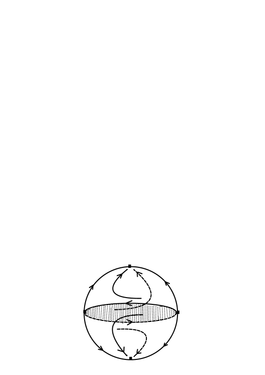
respectively. By Corollary 33 and Remark 34 the central Selgrade bundle $\mathcal{V}_{c}^{1}$ has dimension $\dim\mathcal{V}_{c}^{1}=1+\dim L(0)=2$. Thus $\mathcal{V}_{1}^{\infty}\subset\mathcal{V}_{c}^{1}$ and $\mathcal{V}_{2}^{\infty}$ is a Selgrade bundle at infinity. Inspection of the phase portrait in $\mathbb{R}^{2}$ shows that the unique chain control set $E$ is given by the strip $E=\mathbb{R}\times[-1,1]$. The lift of the chain control set $E$ is the maximal chain transitive set $\mathcal{E}$ for the affine control flow $\Psi$. The orthogonal projection of the system on the northern hemisphere $\mathbb{S}^{2,+}$ to the unit disk yields the phase portrait for $u=\pm 1$ and the chain control set $E_{c}^{1}=\mathbb{P}(E\times\{1\})$ sketched in Fig. 1. The Morse spectra satisfy

$$\Sigma_{Mo}(\mathcal{V}_{1}^{\infty};\Psi^{1})=\Sigma_{Mo}(L(0))=\{0\},\Sigma_{Mo}(\mathcal{V}_{2}^{\infty};\Psi^{1})=\Sigma_{Mo}(L(1))=\{1\},$$

and the inclusion in Theorem 16(ii) implies $0\in\Sigma_{Mo}(\mathcal{V}_{c}^{1};\Psi^{1})$.

In the next example the eigenvalue 00 of the matrix $A$ is not semisimple.

Example 38

Consider

$$\left(\begin{array}[c]{c}\dot{x}\\ \dot{y}\end{array}\right)=\left(\begin{array}[c]{cc}0&1\\ 0&0\end{array}\right)\left(\begin{array}[c]{c}x\\ y\end{array}\right)+\left(\begin{array}[c]{c}1\\ 0\end{array}\right)u(t)\mbox{ with }u(t)\in\Omega=[-1,1].$$

The Lyapunov space is $L(0)=\mathbb{R}^{2}$ which is chain transitive for $u\equiv 0$: The $x$-axis consists of equilibria and for $y\not=0$ all trajectories move on parallels to the $x$-axis (to the right for $y>0$ and to the left for $y<0$). Thus the chain control set $E$ coincides with $\mathbb{R}^{2}$. Note that the $(\varepsilon,T)$-chains become unbounded for $T\rightarrow\infty$. On the equator $\mathbb{S}^{1}\times\{0\}$ of $\mathbb{S}^{2}$ there are two equilibria given by the intersection with the eigenspace $\mathbb{R}\times\{0\}$. For $\Psi^{1}$ there is no Selgrade bundle at infinity and the central Selgrade bundle is $\mathcal{V}_{c}^{1}=\mathcal{U}\times\mathbb{R}^{2}\times\mathbb{R}$. This yields the chain recurrent component $\mathcal{M}_{c}^{1}=\mathbb{P}\mathcal{V}_{c}^{1}=\mathcal{U}\times\mathbb{P}^{2}$, and the chain control set on the projective Poincaré space is $E_{c}^{1}=\mathbb{P}^{2}$.

For a linear flow $\Phi$ Remark 20 characterizes the central Selgrade bundle using the subbundles $\mathcal{V}_{i}$ such that $h^{1}(\mathcal{V}_{i})$ is chain transitive. The following example of a bilinear control system shows that there may exist several subbundles $\mathcal{V}_{i}$ with this property; cf. [6, Example 5.2] which is based on [7, Example 5.5.12].

Example 39

Consider the bilinear control system given by

$$\left(\begin{array}[c]{c}\dot{x}\\ \dot{y}\end{array}\right)=\left[\left(\begin{array}[c]{cc}0&-\frac{1}{4}\\ -\frac{1}{4}&0\end{array}\right)+u_{1}\left(\begin{array}[c]{cc}1&0\\ 0&1\end{array}\right)+u_{2}\left(\begin{array}[c]{cc}0&1\\ 0&0\end{array}\right)+u_{3}\left(\begin{array}[c]{cc}0&0\\ 1&0\end{array}\right)\right]\left(\begin{array}[c]{c}x\\ y\end{array}\right)$$

with

$$u(t)=(u_{1}(t),u_{2}(t),u_{3}(t))\in\Omega=\left[-1,1\right]\times\left[-1/4,1/4\right]\times\left[-1/4,1/4\right]\subset\mathbb{R}^{3}\mbox{.}$$

This defines a linear flow $\Phi_{t}(u,x)=\left(u(t+\cdot),\varphi(t,x,u)\right),t\in\mathbb{R}$, on the vector bundle $\mathcal{U}\times\mathbb{R}^{2}$. With

$$A_{1}=\left\{\left(\begin{array}[c]{c}x\\ \alpha x\end{array}\right)\left|\alpha\in\left[-\sqrt{2},-\frac{1}{\sqrt{2}}\right]\right.\right\},\,A_{2}=\left\{\left(\begin{array}[c]{c}x\\ \alpha x\end{array}\right)\left|\alpha\in\left[\frac{1}{\sqrt{2}},\sqrt{2}\right]\right.\right\},$$

the Selgrade bundles are, for $i=1,2$,

$$\mathcal{V}_{i}=\left\{(u,x,y)\in\mathcal{U}\times\mathbb{R}^{2}\left|\varphi(t,x,y,u)\in A_{i}\mbox{ for }t\in\mathbb{R}\right.\right\}\mbox{ with }\dim\mathcal{V}_{i}=1.$$

One obtains the two chain recurrent components $\mathcal{M}_{i}=\mathbb{P}\mathcal{V}_{i}$ of $\mathbb{P}\Phi$ on the projective bundle $\mathcal{U}\times\mathbb{P}^{1}$ ordered by $\mathcal{M}_{1}\preceq\mathcal{M}_{2}$. The Morse spectra are

$$\mathbf{\Sigma}_{Mo}(\mathcal{V}_{1})=\left[-2,1/2\right]\mbox{ and }\mathbf{\Sigma}_{Mo}(\mathcal{V}_{2})=\left[-1/2,2\right].$$

Since, for $i=1,2$, one has $0\in\mathrm{int}\Sigma_{Mo}(\mathcal{V}_{i})$, Theorem 21 implies that $h^{1}(\mathcal{V}_{i})$ is chain transitive in the projective Poincaré bundle $\mathcal{U}\times\mathbb{P}^{2}$. By Remark 20 the central Selgrade bundle is

$$\mathcal{V}_{c}^{1}=\mathcal{P}\oplus\mathcal{V}_{1}^{\infty}\oplus\mathcal{V}_{2}^{\infty}=\mathcal{U\times}\mathbb{R}^{3},$$

where $\mathcal{P=U}\times\{0\}\times\mathbb{R}\subset\mathcal{U}\times\mathbb{R}^{2}\times\mathbb{R}$ is the polar bundle. There is no Selgrade bundle at infinity.

Acknowledgement. We appreciate the careful reading and the constructive comments of an anonymous reviewer which helped to improve the paper.

7 Declarations

7.1 Funding

No funding received

7.2 Conflict of interest/Competing interests

No interests of a financial or personal nature

7.3 Ethics approval

Not applicable

7.4 Consent to participate

According to
https://www.springer.com/gp/editorial-policies/informed-consent this item it is not applicable

7.5 Consent for publication

According to
https://www.springer.com/gp/editorial-policies/informed-consent this item it is not applicable

7.6 Availability of data and materials

Not applicable

7.7 Code availability

Not applicable

7.8 Authors’ contributions

All authors contributed to all sections. All authors reviewed the final manuscript.

References

  • [1] J.M. Alongi and G.S. Nelson, Recurrence and Topology, Graduate Studies in Math. Vol. 85, Amer. Math. Soc. 2007.
  • [2] M.B. Antunez, G.E. Mantovani, and R. Varão, Chain recurrence and positive shadowing in linear dynamics, J. Math. Anal. Appl. 506(1) (2022), 125622.
  • [3] L.A. Alves and L.A.B. San Martin, Conditions for equality between Lyapunov and Morse decompositions, Ergod. Th. & Dynam. Sys., 36(4) (2016), pp. 1007-1036.
  • [4] A. Blumenthal and Yu. Latushkin, The Selgrade decomposition for linear semiflows on Banach spaces, J. Dyn. Diff. Equations, 31(3) (2019), pp. 1427-1456.
  • [5] I.U. Bronstein and A.Ya. Kopanskii, Smooth Invariant Manifolds and Normal Forms, World Scientific 1994.
  • [6] F. Colonius, On the global behavior of linear flows, Proc. Amer. Math. Soc. 151 (2023), 135-149.
  • [7] F. Colonius and W. Kliemann, The Dynamics of Control, Birkhäuser 2000.
  • [8] F. Colonius and W. Kliemann, Dynamical Systems and Linear Algebra, Graduate Studies in Math. Vol. 156, Amer. Math. Soc. 2014.
  • [9] F. Colonius and A.J. Santana, Topological conjugacy for affine-linear flows and control systems, Communications on Pure and Applied Analysis, 10(3) (2011), 847-857.
  • [10] F. Colonius, A.J. Santana, and J. Setti, Controllability of periodic linear systems, the Poincaré sphere, and quasi-affine systems, Math. Control, Signals, Syst. (2023), doi.org/10.1007/s00498-023-00369-y.
  • [11] D.L. Elliott, Bilinear Control Systems, Matrices in Action, Kluwer Academic Publishers, 2008.
  • [12] L. Grüne, A uniform exponential spectrum for linear flows on vector bundles, J. Dyn. Diff. Equations, 12 (2000), pp. 435-448.
  • [13] R.A. Johnson, K.J. Palmer and G.R. Sell, Ergodic properties of linear dynamical systems, SIAM J. Math. Anal., 18 (1987), pp. 1-33.
  • [14] C. Kawan, Invariance Entropy for Deterministic Control Systems, Lect. Notes Math. Vol 2089, Springer 2013.
  • [15] C. Kawan and T. Stender, Growth rates for semiflows an Hausdorff spaces, J. Dyn. Diff. Equations, 24(2) (2012), pp. 369-390.
  • [16] P.E. Kloeden and M. Rasmussen, Nonautonomous Dynamical Systems, Amer. Math. Soc. 2011.
  • [17] J.L. Massera and J.J. Schäffer, Linear Differential Equations and Function Spaces, Academic Press 1966.
  • [18] M. Patrao and L.A.B. San Martin, Morse decomposition of flows and semiflows on fiber bundles, Disc. Cont. Dyn. Syst., 17 (2007), 113-139.
  • [19] L. Perko, Differential Equations and Dynamical Systems, Springer, 3rd ed., 2001.
  • [20] H. Poincare, Memoire sur les courbes definies par une equation differentielle, J. Mathematiques, 7 (1881), pp. 375-422; Ouevre Tome I, Gauthier-Villar, Paris 1928, pp. 3-84.
  • [21] C. Robinson, Dynamical Systems: Stability, Symbolic Dynamics, and Chaos, Taylor & Francis Inc., 2nd ed., 1998.
  • [22] R.J. Sacker and G.R. Sell, A spectral theory for linear differential equations, J. Diff. Equations, 27 (1978), pp. 320-358.
  • [23] D. Salamon and E. Zehnder, Flows on vector bundles and hyperbolic sets, Trans. Amer. Math. Soc., 306 (1988), pp. 623-649.
  • [24] J. Selgrade, Isolated invariant sets for flows on vector bundles, Trans. Amer. Math. Soc., 203 (1975), pp. 259-390.
  • [25] E. Sontag, Mathematical Control Theory, Springer-Verlag 1998.
Refer to caption
Figure 1: Chain control set $E_{c}^{1}$ and phase portraits for $u=\pm 1$ in Example 37.