Scalable regression calibration approaches to correcting measurement error in multi-level generalized functional linear regression models with heteroscedastic measurement errors

Abstract

Wearable devices permit the continuous monitoring of biological processes, such as blood glucose metabolism, and behavior, such as sleep quality and physical activity. The continuous monitoring often occurs in epochs of 60 seconds over multiple days, resulting in high dimensional longitudinal curves that are best described and analyzed as functional data. From this perspective, the functional data are smooth, latent functions obtained at discrete time intervals and prone to homoscedastic white noise. However, the assumption of homoscedastic errors might not be appropriate in this setting because the devices collect the data serially. While researchers have previously addressed measurement error in scalar covariates prone to errors, less work has been done on correcting measurement error in high dimensional longitudinal curves prone to heteroscedastic errors. We present two new methods for correcting measurement error in longitudinal functional curves prone to complex measurement error structures in multi-level generalized functional linear regression models. These methods are based on two-stage scalable regression calibration. We assume that the distribution of the scalar responses and the surrogate measures prone to heteroscedastic errors both belong in the exponential family and that the measurement errors follow Gaussian processes. In simulations and sensitivity analyses, we established some finite sample properties of these methods. In our simulations, both regression calibration methods for correcting measurement error performed better than estimators based on averaging the longitudinal functional data and using observations from a single day. We also applied the methods to assess the relationship between physical activity and type 2 diabetes in community dwelling adults in the United States who participated in the National Health and Nutrition Examination Survey.

Basis splines; Diabetes; Functional data; Physical activity; Splines; Wearable accelerometer

1 INTRODUCTION

Wearable monitoring devices permit the continuous monitoring of biological processes, such as blood glucose metabolism (Tsai and others, 2019; Gaynanova and others, 2022), and behavior, such as sleep quality (Kuo and others, 2016; Tuominen and others, 2019) and physical activity (Troiano and others, 2008). The continuous monitoring often occurs in epochs of 60 seconds over multiple days resulting in high dimensional longitudinal curves that are best described and analyzed as functional data.

While researchers have previously addressed measurement error in scalar covariates prone to error (Carroll and others, 2006), less work has been done on correcting measurement error in high dimensional longitudinal curves prone to complex heteroscedastic errors (Cardot and others, 2007; Crambes and others, 2009; Goldsmith and others, 2011). When correcting for measurement error, functional data analysts have previously assumed that the serially observed functional data represent a curve of a latent process contaminated by noise with an independent error structure (Silverman and Ramsay, 2005). Because observation periods for functional data often extend over multiple days, it is necessary to develop methods for correcting measurement error in serially observed data prone to complex heteroscedastic error structures. Prior approaches to correcting measurement error in serially observed functional data prone to complex errors involve the assumption that the observed curves are from the normal distribution (Tekwe and others, 2022; Jadhav and others, 2022). However, sometimes the curves might be best described as belonging in more flexible distributions such as those in the exponential family (Crainiceanu and others, 2009). To address these limitations, we propose two regression calibration approaches for correcting measurement error in longitudinal functional data from the exponential family of distributions and prone to complex heteroscedastic measurement error.

In our current work, we seek to assess the role of physical activity in type 2 diabetes (T2D). The incidence and prevalence of T2D have increased over the past 20 years. Over one-third of U.S. adults are obese, and $\geq$ 11% of people over 20 years old have T2D (Eckel and others, 2011). Some researchers project that the overall prevalence of T2D in the U.S. will be 21% by 2050 (Boyle and others, 2010). Obesity results from a chronic imbalance between energy intake and energy expenditure (Spiegelman and Flier, 2001). To combat the growing epidemic of obesity and its associated health outcomes such as T2D, clinicians and researchers have proposed treatments to reduce dietary intake and increase daily physical activity (Balk and others, 2015). Therefore, it is critical to assess these behaviors accurately and evaluate how they influence obesity and T2D. Self-reported measures of physical activity are prone to recall bias (Sallis and Saelens, 2000; Armstrong and Bull, 2006). Consequently, researchers increasingly use wearable devices to monitor physical activity (Kozey and others, 2010). Wearable devices for physical activity are based on motion sensor technology and data processing to provide measures of physical activity frequency, duration, and intensity (Kozey and others, 2010; Troiano and others, 2008). While wearable device measures of physical activity are not prone to recall and researcher bias, their accuracy may be questionable (Bassett, 2012; Crouter and others, 2006; Jacobi and others, 2007; Warolin and others, 2012; Rothney and others, 2008; Kozey and others, 2010). The sources of error in wearable device measures of physical activity are both random and systematic. To process accelerometer data from wearable devices, the devices must first be calibrated to record activity counts with another physiological variable, such as the metabolic equivalent task (MET)(Kozey and others, 2010; Crouter and others, 2006; Swartz and others, 2000). Next, the device approximates activity counts from its relationship with the physiological variable with a regression equation (Kozey and others, 2010). However, there are currently no standard equations, with over 30 equations available for this estimation (Plasqui and Westerterp, 2007; Kozey and others, 2010; Crouter and others, 2006; Rothney and others, 2008). The accuracy of the data generated by the devices thus depends on the estimation equations. The accuracy also depends on the activity type, sex, and body composition of device users (Freedson and others, 1998; Valenti and others, 2014). In short, physical activity is a latent variable not observed directly but represented by a proxy, the wearable device measure. Such surrogate measurement tends to introduce measurement error (Carroll and others, 2006).

We present fast, scalable regression calibration methods for correcting measurement error in functional covariates in multi-level generalized functional linear regression models with complex heteroscedastic measurement errors. Our new methods have several advantages. First, we assume the distributions of the device-based measures of physical activity belong in the exponential family. This allows for a more general specification of the distributions of the device-based measures compared to current approaches that often entail assumptions of normality for these surrogate measures. Second, we treat the random errors in the surrogate measures as complex heteroscedastic errors from the Gaussian distribution with covariance error functions. Third, our methods can be used to evaluate relationships between multi-level functional covariates with complex measurement error structures and scalar outcomes with distributions in the exponential family. Fourth, we treat the functional covariate as a surrogate measure for true functional covariate. We also report on our application of the new methods to assess the relationship between physical activity and T2D in data from the National Health and Nutrition Examination Survey (NHANES).

2 GENERALIZED FUNCTIONAL REGRESSION WITH MULTI-LEVEL HETEROSCEDASTIC MEASUREMENT ERRORS

2.1 The model

Let $\mathcal{D}_{i}=\{Y_{i},{\mathbf{W}}_{i},{\mathbf{Z}}_{i}\}$ be a triplet for individual $i(i=1,\dots,n)$ consisting of, respectively, a scalar outcome $Y_{i}$, a functional covariate measured at multiple time points which we denote as ${\mathbf{W}}_{i}=\{W_{ij}(t)\}^{t\in T_{i}}_{j=1,\cdots,J}\in\mathbb{R}^{T_{i}\times J}$, where $T_{i}$ is the number of distinct time points at which the covariates $W_{ij}(t)$ are measured, and ${\mathbf{Z}}_{i}\in\mathbb{R}^{p}$ is a vector of length $p$ representing the error-free covariates. For example, $Y_{i}$ could represent a health outcome such as T2D status and ${\mathbf{W}}_{i}$ could represent physical activity curves obtained from a monitoring device. Our model for the $i$th subject is as follows:

$$g[E\{Y_{i}\mid X_{i}(t),{\mathbf{Z}}_{i}\}] = \int_{0}^{1}\beta(t)X_{i}(t)dt+{\mathbf{Z}}_{i}^{\rm T}\mbox{\boldmath$\alpha$},$$ (1)

$$h[E\{W_{ij}(t)\}] = X_{i}(t)+U_{ij}(t);$$ (2)

where $g(\bullet)$ and $h(\bullet)$ are both monotone, twice continuously differentiable functions; and $X_{i}(t)$ is a latent functional covariate with its associated unknown functional coefficient, $\beta(t)$. The response variable $Y_{i}$ may be either a continuous or discrete outcome with a distribution belonging in the exponential family; $\alpha$ is a $p\times 1$ vector of coefficients associated with the $p$ error-free covariates, ${\mathbf{Z}}_{i}$. Further, $W_{ij}(t)$ is the $t$th $t=(1,\ldots,T)$ observation collected at the $j$th $j=(1,\ldots,J)$ day for subject $i$. Let $X_{i}(t)$ be a functional covariate that is not directly observable but approximated by $W_{ij}(t)$ with some error. The random terms or intercepts, $U_{ij}(t)$, in Equation 2 are subject-specific deviations of the observed data, $W_{ij}(t)$, from their overall mean functions, $X_{i}(t)$. Equations 1 and 2 represent the systematic component of a generalized functional linear model with the random component left completely unspecified for now. The exponential family specification of the measurement error component of the model is a significant departure from current approaches that are based on Gaussian processes.

3 ESTIMATION AND INFERENCE

Estimation and inference about the functional parameter $\beta(t)$ is our primary goal. However, $X_{i}(t)$ is latent and not directly observed. Estimating $\beta(t)$ with the observed measure of $X_{i}(t)$, $W_{ij}(t)$, leads to biased estimates of $\beta(t)$ (Carroll and others, 2006). The biased estimator of $\beta(t)$ may attenuate or over-estimate the true effects of $X_{i}(t)$ depending on the regression model. However, the presence of some additional information in the data, such as validation data, repeated measurements on $W_{ij}(t)$, or instrumental variables for $X_{i}(t)$, may be used to correct for the biases due to measurement errors (Carroll and others, 2006). Given additional identifying information, estimation approaches such as regression calibration may be used to obtain unbiased estimators for $\beta(t)$. Regression calibration is a bias correction method that substitutes $E\{X_{i}(t)\mid W_{ij}(t),{\mathbf{Z}}_{i}\}$ for $X_{i}(t)$ in Equation 1. We use replicates for identifying the model and regression calibration for correcting measurement error.

Most methods for correcting measurement error in functional data (Tekwe and others, 2019) require approximating the functional parameters and covariates in Equations 1 and 2 prior to estimation. However, with our new methods, we first perform point-wise generalized linear mixed effects analysis of $W_{ij}(t)$ by $t$, the time of observation, a process called massive univariate analysis (Cui and others, 2021). This step yields predicted values for $X_{i}(t)$, the fixed component of the measurement error model in Equation 2. The use of generalized linear mixed effects models to obtain the predicted values for $X_{i}(t)$ is possible due to the repeated measures on $W_{ij}(t)$ across the $J$ days. In the second step, we smooth the predicted values of $X_{i}(t)$, $\hat{X}_{i}(t)\mid{\mathbf{U}}_{ij}(t)$ across $t$ with any smoother, such as Bsplines or penalized splines. In the third step, we substitute these values for $X_{i}(t)$ in the regression equations for the outcome in Equation 1. The last step involves nonparametric bootstraps to estimate confidence bands.

3.1 Likelihood

Given the observed data $\mathcal{D}_{i}=\{Y_{i},{\mathbf{W}}_{i},{\mathbf{Z}}_{i}\}$, the contribution of individual $i$ to the likelihood, $\ell_{i}$, is equal to

$$\ell_{i}\{{\mathbf{X}}_{i},\beta(t),\mbox{\boldmath$\alpha$},\mbox{\boldmath$\theta$}_{w}\} = f_{y}(Y_{i}|\beta(t),\mbox{\boldmath$\alpha$},{\mathbf{X}}_{i},{\mathbf{Z}}_{i})\prod^{J}_{j=1}f_{W}({\mathbf{W}}_{ij}|{\mathbf{X}}_{i},\mbox{\boldmath$\theta$}_{w}),$$ (3)

where $f_{y}(\bullet)$ and $f_{w}(\bullet)$ are densities from the exponential family which depend on the choice of the link function and the random component. We note that the likelihood specified in Equation 3 is flexible as it allows for non-normal data. For example, with an identity function that has Gaussian random components for $h(\bullet)$ and $g(\bullet)$, our model becomes the usual Gaussian measurement error model. The joint likelihood then is

$$\ell = \prod^{n}_{i=1}\ell_{i}\{{\mathbf{X}}_{i},\beta(t),\mbox{\boldmath$\alpha$},\mbox{\boldmath$\theta$}_{w}\}.$$ (4)

In likelihoods 3 and 4, the functional covariate ${\mathbf{X}}_{i}=\{X_{i}(t)\}^{i\in n}$ is a random function because it is unknown and unobserved, which is characteristic of the scalar-on-function regression with measurement error (Tekwe and others, 2019).

3.2 Model assumptions

To estimate the model parameters, we assume the following:

• ] $Y_{i}\sim EF(\bullet)$, where EF refers to an exponential family distribution.

• ] The functions, $g(\bullet)$ and $h(\bullet)$, are monotone, twice continuously differentiable functions.

• ] $\mathrm{h[{E}}\{W_{ij}(t)\mid X_{i}(t)\}]=X_{i}(t)$, and if $h(\bullet)$ is the identity function, then $\mathrm{{E}}\{W_{ij}(t)\mid X_{i}(t)\}=X_{i}(t)$.

• ] $\mathrm{Cov}\{W_{ij}(t),X_{i}(t)\}\neq 0$.

• ] $\mathrm{Cov}\{X_{i}(t),X_{i}(t^{\prime})\}\neq 0$ and $\mathrm{Cov}\{W_{ij}(t),W_{ij}(t^{\prime})\}\neq 0$ for $t\neq t^{\prime}$.

• ] $W_{ij}(t)|{\cal X}_{i}(t)\sim EF(\bullet)$.

• ] $f\{Y_{i}|X_{i}(t),W_{ij}(t)\}=f\{Y_{i}|X_{i}(t)\}$.

• ] $U_{ij}(t)\sim MVN(0,\Sigma_{uu})$, $\mathrm{Cov}\{U_{ij}(t),U_{ij^{\prime}}(t)\}\neq 0$ for $j\neq j^{\prime}$, and $\mathrm{Cov}\{U_{ij}(t),U_{ij}(t^{\prime})\}\neq 0$ for $t\neq t^{\prime}$.

A1 indicates that the scalar response may be discrete or continuous with a distribution belonging in the EF. A2 includes the usual assumptions for link functions in generalized linear regression models. A3 indicates that nonlinear functions of $\mathrm{E}\{W_{ij}(t)\mid X_{i}(t)\}$ are unbiased measures of $X_{i}(t)$. A4 states that the surrogate measures and the true unobserved covariate are correlated, a classical assumption in measurement error models. A5 and A6 indicate correlated measurement errors for the surrogate measures and the true covariate for each subject $i$. A7 is the non-differential measurement error assumption specifying that the surrogate measure, $W_{ij}(t)$, does not provide any additional information about the response, $Y_{i}$, beyond the information given by $X_{i}(t)$. A8 indicates that subject-specific intercept or deviation of the surrogate measures from the true covariates have Gaussian distributions. Additionally, the covariance function for $U_{ij}(t)$ is correlated across the $J$ days of observation and also across the wear times, $t$.

4 REGRESSION CALIBRATION

Regression calibration (Carroll and others, 2006) is an approach to correcting classical measurement error in regression models with additional identifying data. The method requires a gold standard for the true unobserved covariate, repeated measurements of the observed covariate, or an instrumental variable for the true covariate (Carroll and others, 2006). Researchers have developed maximum likelihood (Spiegelman and Casella, 1997), semiparametric (Pepe and Fleming, 1991; Ye and others, 2008), Bayesian (Bartlett and Keogh, 2018; Zoh and others, 2022), and Monte Carlo (Li and others, 2007; Fearn and others, 2008; Tekwe and others, 2014) approaches to correcting measurement error with regression calibration.

We describe two approaches to using repeated measures for correcting measurement error. Under the assumption that $\hat{E\{X_{ij}(t)\}}=\hat{h[E\{W_{ij}(t)\}]}$, the predicted values from regressing $h[E\{W_{ij}(t)\}]$ on the intercept may be used as calibrated values for ${\mathbf{X}}_{i}$ when assessing its association with the outcome of interest such as in Equation 1. In our approaches, regression calibration proceeds in four steps:

1. Fit the model

   $$h\{X_{i}(t)\} = \gamma_{x}(t)+\varepsilon_{xi}(t),$$ (5)

   where $\gamma_{x}(t)$ is the fixed intercept or mean function for $X_{i}(t)$ at time $t$ and $\varepsilon_{ix}(t)$ is the random error term in the model. We assume $\varepsilon_{ix}(t)\sim MVN\{0,\Sigma_{xx}(t,t^{\prime})\}$, for $t\neq t^{\prime}$. However, we cannot fit the model in Equation 5 because $X_{i}(t)$ is latent and unobserved. We therefore replace $X_{i}(t)$ with $W_{ij}(t)$, its unbiased but measurement error-prone observed measure. Following this replacement Equation 5 becomes

   $$h[E\{W_{ij}(t)\}] = \gamma_{w}(t)+U_{ij}(t),$$ (6)

   where $\gamma_{w}(t)$ is the fixed intercept and $U_{ij}(t)$ is the subject-specific random intercept. We assume $U_{ij}(t)\sim MVN\{0,\Sigma_{uu}(t,t^{\prime})\}$ for $t\neq t^{\prime}$.

2. Replace $X_{i}(t)$ with $\hat{h[\{W_{ij}(t)\}]}$ obtained from the predicted values in Equation 6. Most current approaches to correcting measurement error in functional data analysis with functional covariates prone to measurement error require some dimension reduction before correcting measurement error. However, the regression calibration methods we propose do not require dimension reduction of $W_{ij}(t)$ to obtain predicted values of $X_{i}(t)$ for fitting the regression model in Equation 1.

3. While dimension reduction is not required to obtain the measurement error-corrected measure of $X_{i}(t)$, we do reduce dimensions in the regression step. Using $\hat{h[\{W_{ij}(t)\}]}$ for $X_{i}(t)$ in Equation 1, we reduce the dimensions of the functional terms by approximating them with polynomial splines $\beta(t)\approx\sum_{k=1}^{K_{n}}\omega_{k}b_{k}(t)$ and $\hat{h[\{W_{ijk}\}]}\approx\int_{0}^{1}\hat{h[\{W_{ij}(t)\}]}b_{k}(t)dt$, where $\left\{\omega_{k}\right\}_{k=1}^{K_{n}}$ are unknown spline coefficients and $\left\{b_{k}(t)\right\}_{k=1}^{K_{n}}$ are a set of spline basis functions on $[0,1]$. Equation 1 becomes

   $$g[E\{Y_{i}\mid{\mathbf{X}}_{i},{\mathbf{Z}}_{i}\}] \approx \sum_{k=1}^{K_{n}}\omega_{k}\hat{h[\{W_{ijk}\}]}+{\mathbf{Z}}_{i}^{\rm T}\mbox{\boldmath$\alpha$}.$$ (7)

4. Maximize the likelihood function in the reduced form model in Equation 7 by replacing ${\mathbf{X}}_{i}$ with $\hat{h[\{W_{ijk}\}]}$ to obtain estimated model parameters $E\{\hat{\beta}(t)\}\approx E\{\sum_{k=1}^{K_{n}}\hat{\omega}_{k}b_{k}(t)\}$ and $E(\hat{\mbox{\boldmath$\alpha$}})=\mbox{\boldmath$\alpha$}$.

Our methods for correcting measurement error allow arbitrary error structures for $\Sigma_{uu}(t,t^{\prime})$, such as unstructured, compound symmetry, or autoregressive 1. We propose two regression calibration approaches. For our first approach, we adapt the fast univariate inference (FUI) modeling developed by Cui and colleagues (Cui and others, 2021) to implement the functional analog of regression calibration. Using the repeated measurements on $W_{ij}(t)$ as additional identifying information for estimating $\Sigma_{uu}(t,t^{\prime})$, FUI treats the repeated functional measures across multiple days as longitudinal high dimensional data and fits a point-wise generalized linear mixed effects model at each wear time $t,t=1,\ldots,T$ across all the $J$ observational periods or days resulting in $T$ estimated fixed effects. The term ”univariate” in FUI refers to the point-wise fitting for each wear time separately. We use the predicted values from these point-wise generalized linear mixed effects models as replacement values for $X_{i}(t)$.

A potential drawback of the FUI method is that it may not account for the serial correlation across days or observation periods adequately due to its univariate focus. Therefore, we propose a fast short multivariate inference approach (FSMI). The FSMI method also involves fitting point-wise generalized linear mixed effects models to the data with Equation 6, but by analyzing observations from multiple wear times concurrently and proceeding across all the $T_{i}$ wear times in a moving average. The term ”multivariate” here refers to the use of multiple wear times concurrently in fitting the point-wise generalized linear mixed effects model.

For inference, we used $95\%$ nonparametric point-wise bootstrap confidence intervals.

5 SIMULATIONS

We conducted simulations to investigate the finite sample properties of our methods. We generated 1,000 data sets with sample sizes $n\in(100,200,500,1,000,2,000,5,000)$ independently from the model in Equation 1 using an identity function for $g(\bullet)$. We simulated the outcomes as $Y_{i}\sim Binomial(p_{i})$ with $p_{i}=expit(\eta_{i})$ and $\eta_{i}=\int_{0}^{1}\beta(t)X_{i}(t)dt+\boldsymbol{Z_{i}\alpha}$, where $\beta(t)=sin(2\pi t)$ and $\boldsymbol{\alpha}=(1,2)$. We simulated the true functional covariate with $X_{i}(t)=1/[1+\exp\{8(t-0.5)\}]+\epsilon_{X}(t)$, and generated $\epsilon_{X}(t)$’s independently from a Gaussian process (GP) with mean 0 and an autoregressive one structure for the covariance matrix. Thus, $\epsilon_{X}(t)\sim GP\{\boldsymbol{0},\Sigma_{xx}(t,t^{\prime})\}$ for $t\neq t^{\prime}$. We included a continuous error-free covariate, $Z_{1i}$, and a binary error-free covariate, $Z_{2i}$, simulated independently with $Z_{1i}\sim N(2,1)$ and $Z_{2i}\sim Binomial(1,0.6)$, respectively. We generated the surrogate measure, $W_{ij}(t)$, from a Poisson process (PP) with mean function $\lambda_{i}(t)$. That is, $W_{ij}(t)\sim PP\{\lambda_{i}(t)\}$, where $\lambda_{i}(t)=\exp\{X_{i}(t)\}$ and $j=1,\dots,J=5$. The measurement error component of our model in Equation 2 was $\hbox{log}[E\{W_{ij}(t)\}]=X_{i}(t)+U_{ij}(t)$ for the $i$th subject at the $j$th replication, and we assumed $U_{ij}(t)\sim GP\{\boldsymbol{0},\Sigma_{uu}(t,t^{\prime})\}$ for $t\neq t^{\prime}$.

We compared five estimators for $\beta(t)$ in Equation 1 in analyzing the simulated data: FUI, FSMI, average, naive, and oracle. The average estimator averages the repeatedly observed surrogate for $X_{i}(t)$ across the $J$ replicates to obtain $\bar{W}_{i\bullet}(t)$. The naive estimator is based on the first replicate $\{W_{i1}(t)\}$ of the surrogate measures as a substitute for $X_{i}(t)$. The oracle or benchmark estimator uses $X_{i}(t)$. The average method provides an ad hoc method for reducing bias due to measurement error, while the naive estimator does not correct for any measurement error.

We performed three sets of simulations to investigate the performance of the five estimators in response to three different factors, respectively: 1) increasing sample size, with $n\in(100,200,500,1,000,2,000,5,000)$, $\sigma_{x}=3.0$, where $\sigma_{x}$ indicates the diagonal elements in the covariance matrix for $X_{i}(t)$, and $\rho_{x}=0.50$; 2) the increasing magnitude of the measurement error with $n=5,000$, $\sigma_{x}\in(1.5,2.0,3.0)$, and $\rho_{x}=0.75$; and 3) increasing magnitude of the serial correlation across time points for $X_{i}(t)$ with $\rho_{x}\in(0.05,0.25,0.5,0.75)$, $n=5,000$, and $\sigma_{x}=3.0$. All simulations were conducted with 1,000 iterations.

We compared the estimators with three measures. Let $\hat{\beta}^{r}(t)$ be the estimator of $\beta(t)$ at the $r$th $(r=1,\ldots,R)$ simulation replicate and $\bar{\beta}(t)=\frac{1}{R}\sum_{r=1}^{R}\hat{\beta}^{r}(t)$, the averaged estimate over a total of $R=1,000$ replications. Let $\left\{t_{l}\right\}_{l=1}^{n_{grid}}$ be a sequence of equally spaced grid points on $[0,1]$. We define the average squared bias (ABias²) of $\hat{\beta}(t)$, the average sample variance (AVar), and the average integrated mean square error (AIMSE) as

$$\text{ABias}^{2}\{\hat{\beta}(t)\} = \frac{1}{n_{grid}}\sum_{l=1}^{n_{grid}}\{\bar{\beta}(t_{l})-{{{\beta_{true}(t_{l})}}}\}^{2},$$

$$\text{AVar}\{\hat{\beta}(t)\} = \frac{1}{R}\sum_{r=1}^{R}\frac{1}{n_{grid}}\sum_{l=1}^{n_{grid}}\left\{\hat{\beta}^{r}(t_{l})-\bar{{\beta}}(t_{l})\right\}^{2},\text{and}$$

$$\text{AIMSE}\{\hat{\beta}(t)\} = \text{ABias}^{2}\{\hat{\beta}(t)\}+\text{AVar}\{\hat{\beta}(t)\},\text{respectively.}$$

Small values of these measures indicate good performance and large values indicate poor performance.

5.1 Simulation results

5.1.1 Impact of sample size

Table 1 summarizes the results for varying sample size. As the sample size increased, the ABias², AVar, and AIMSE consistently decreased for all the estimators. The FSMI estimator had ABias² consistently smaller than that of the FUI, average, and naive estimators and closest to that of the oracle estimator. The oracle estimator had the smallest Avar, followed in order by the FSMI, FUI, naive, and the average method. Similarly, the average method had the highest values for AIMSE while the AIMSE associated with the oracle estimator was the smallest.

Table 1: The effect of varying sample size on the performance of $\hat{\beta}(t)$ under the five estimators with $n\in(100,200,500,1,000,2,000,5,000)$, $\sigma_{x}=3.0$, and $\rho_{x}=0.50$.

	ABias2					AVar					AIMSE
n	Oracle	FSMI	FUI	Average	Naive	Oracle	FSMI	FUI	Average	Naive	Oracle	FSMI	FUI	Average	Naive
100	0.0079	0.0174	0.0297	0.2942	0.2097	3.2800	3.8213	4.2202	9.0955	8.4759	3.2879	3.8387	4.2499	9.3897	8.6856
200	0.0016	0.0056	0.0129	0.2132	0.1520	1.4365	1.6621	1.8318	3.9350	3.6675	1.4381	1.6677	1.8447	4.1482	3.8196
500	0.0009	0.0023	0.0067	0.1686	0.1185	0.6369	0.7418	0.8155	1.7658	1.6114	0.6378	0.7440	0.8222	1.9344	1.7300
1000	0.0002	0.0019	0.0067	0.1761	0.1247	0.3605	0.4177	0.4571	0.9729	0.9109	0.3607	0.4195	0.4638	1.1490	1.0357
2000	0.0001	0.0015	0.0061	0.1727	0.1220	0.2111	0.2449	0.2661	0.5614	0.5163	0.2112	0.2464	0.2722	0.7341	0.6384
5000	0.0001	0.0014	0.0060	0.1705	0.1220	0.1092	0.1280	0.1378	0.2931	0.2670	0.1093	0.1294	0.1437	0.4636	0.3890

5.1.2 Impact of the magnitude of measurement error

Table 2 provides the results on varying levels of the magnitude of measurement error. The oracle estimator consistently had the smallest Abias² and AVar of the five estimators. The FSMI estimator had the next smallest Abias² and AVar values, followed by, in ascending order, the FUI, naive, and average estimators. The oracle estimator had the smallest values of Avar and AIMSE while the FSMI estimator had the second smallest values.

Table 2: The effect of varying magnitude of measurement error on the performance of $\hat{\beta}(t)$ for the five estimators with $n=5,000$, $\sigma_{x}\in(1.5,2.0,3.0)$, and $\rho_{x}=0.75$

	ABias2					AVar					AIMSE
$\sigma_{x}$	Oracle	FSMI	FUI	Average	Naive	Oracle	FSMI	FUI	Average	Naive	Oracle	FSMI	FUI	Average	Naive
1.5	0.0001	0.0017	0.0078	0.1791	0.1519	0.1100	0.1280	0.1349	0.2820	0.2564	0.1102	0.1298	0.1426	0.4611	0.4083
2.0	0.0000	0.0026	0.0079	0.1820	0.1686	0.0648	0.0761	0.0796	0.1653	0.1567	0.0648	0.0787	0.0875	0.3473	0.3253
3.0	0.0000	0.0048	0.0103	0.1824	0.1772	0.0294	0.0367	0.0383	0.0778	0.0759	0.0294	0.0415	0.0486	0.2602	0.2531

5.1.3 Impact of the strength of serial correlation across time points

Table 3 summarizes the impacts of the varying strength of the serial correlation across time points for the functional covariate, $X_{i}(t)$. The simulation results demonstrate that the biases associated with the oracle, FSMI, and FUI methods were all smaller than those obtained under the average and naive approaches. The strength of correlation of the functional covariate did not affect the estimators obtained under the oracle and FSMI methods as their ABias²’s remained more stable for increasing values of $\rho_{x}$. As the correlation coefficient, $\rho_{x}$, increased, the Avar and AIMSE of all five estimations decreased. The oracle estimator had the smallest values of Avar and AIMSE and followed in decreasing order by the FSMI, FUI, average, and naive estimators.

Table 3: The effect of increasing magnitude of the serial correlation cross time points for $X_{i}(t)$ on the performance of $\hat{\beta}(t)$ for the five estimators with $\rho_{x}\in(0.05,0.25,0.5,0.75)$, $n=5,000$, and $\sigma_{x}=3.0$.

	ABias2					AVar					AIMSE
$\rho_{x}$	Oracle	FSMI	FUI	Average	Naive	Oracle	FSMI	FUI	Average	Naive	Oracle	FSMI	FUI	Average	Naive
0.05	0.0001	0.0039	0.0044	0.1146	0.0989	0.0519	0.0667	0.0673	0.1389	0.1349	0.0520	0.0706	0.0716	0.2535	0.2338
0.25	0.0000	0.0043	0.0068	0.1507	0.1370	0.0378	0.0478	0.0497	0.1041	0.1025	0.0378	0.0521	0.0565	0.2547	0.2395
0.50	0.0000	0.0052	0.0099	0.1799	0.1703	0.0285	0.0358	0.0378	0.0793	0.0777	0.0285	0.0410	0.0478	0.2592	0.2479
0.75	0.0000	0.0048	0.0103	0.1824	0.1772	0.0294	0.0367	0.0383	0.0778	0.0759	0.0294	0.0415	0.0486	0.2602	0.2531

6 APPLICATION

6.1 Data and Model

We applied our methods to data from the 2005–2006 cycle of the NHANES to assess the association between wearable device-based physical activity (PA) and T2D status while adjusting for age, sex, and race/ethnicity in community-dwelling adults in the U.S. The participants wore ActiGraph uniaxial accelerometers (model #AM7164) on their hips for at least five days during waking hours except during water-related activities, as the ActiGraph devices were not water-proof. The ActiGraph uniaxial accelerometers (model #AM7164) registered PA intensity and step counts as zero when participants were not wearing them or were sedentary. In this application, we define the latent variable, $X_{i}(t)$, as the true unknown activity counts for a given participant $i$ during wear time $t$. The surrogate measure for $X_{i}(t)$ was the step count recorded by the device. Because NHANES did not provide any information to distinguish between non-wear and non-moving time, we defined non-wear time to be when the device-based PA measures were recorded as zero for at least 60 consecutive minutes and set the PA measures (step counts) to be non-applicable values during the non-wear time. We included data on participants who were older than 20 and had PA data for at least two days. We applied sample weights to account for the oversampling of racial subgroups, which were Hispanic and black racial groups, per NHANES guidelines (Johnson and others, 2013). The final analytic sample included 2,001 participants, whose average age was 44 ± 14 years. Fifty-one percent were female and approximately $14\%$ were black, $13\%$ were Hispanic, $68\%$ were white, and $4\%$ were of another race or ethnicity after adjusting for oversampling from some racial groups.

We classified participants who reported they had ever been told by a doctor that they have T2D as having a prior diagnosis of T2D, and classified others as not having such a diagnosis. Figure 1 illustrates patterns of wearable-device-based step counts for weekdays and weekends by time (hours) over 24 hours. The patterns of step counts on weekdays and weekends were similar. Therefore, we analyzed the data for weekdays and weekends together as a whole.

We considered the following functional logistic regression model with measurement error:

$$\hbox{log}\left(\frac{P_{i}}{1-P_{i}}\right) =\int_{0}^{1}\beta(t)X_{i}(t)dt+{\mathbf{Z}}_{i}^{\rm T}\mbox{\boldmath$\alpha$}\text{ and}$$

$$h[E\{W_{ij}(t)\}] =X_{i}(t)+U_{ij}(t),$$

where $P_{i}$ is the probability of being diagnosed with T2D for the $i$th subject, $\beta(t)$ is the unknown functional regression coefficient, and $\alpha$ is the unknown scalar regression coefficients of the error-free covariates. The $X_{i}(t)$ are the unobservable true activity counts, with surrogate measure, $W_{ij}(t)$, representing device-based step counts prone to measurement error, and ${\mathbf{Z}}_{i}$ are the error-free covariates, including age, sex, and race/ethnicity, for the $i$th subject.

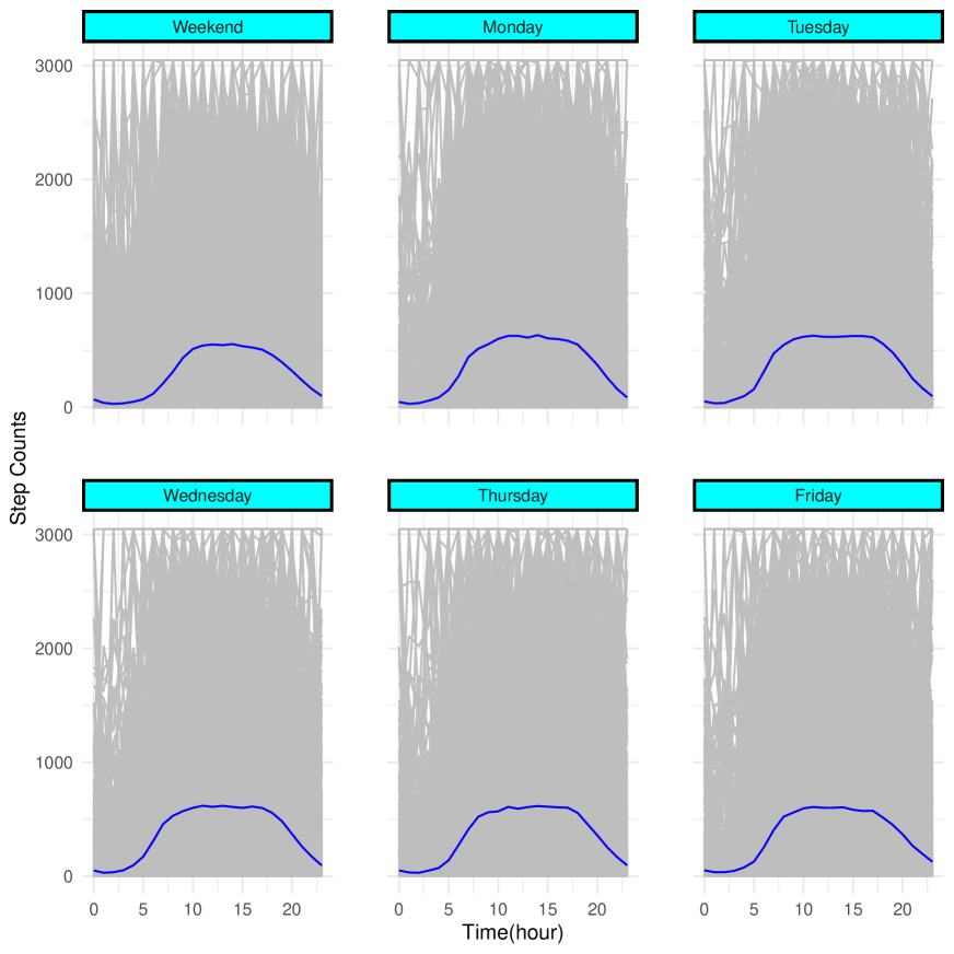
Figure 1: Wearable-device-based step counts from the 2005-2006 NHANES plotted against time (hour) for weekdays and weekends. The grey lines on the background are the trend of step counts over time for each subject and the blue line is the average step count across all participants over time for each day

6.2 Application Results

Table 4 shows the estimated exponentiated regression coefficients of the error-free covariates and their corresponding $95\%$ confidence intervals (CIs) for the FSMI, FUI, average, and naive estimators of $\beta(t)$. We obtained the $95\%$ CIs via a nonparametric bootstrap with $1,000$ replicates. Correcting for measurement error influenced estimates for some error-free covariates but not others. For example, the statistically significant estimates of the age coefficient were similar for the four estimators. There was no statistically significant difference in the odds of T2D between the male and female participants based on all four estimates. Additionally, the regression calibration- and naive-based estimators were smaller than that obtained from the average-based method. There was an increased odds of T2D among blacks when compared to whites. The estimated odds obtained under the FSMI and FUI methods were smaller than those obtained under the average and naive approaches. However, the largest estimated difference in odds of T2D between blacks and whites was based on the average approach. We also observed an increased odds of T2D among Hispanics when compared with whites. While the estimated difference in odds between whites and Hispanics were found to be equivalent based on the FSMI and FUI methods, the average-based was smallest among all four methods. Finally, we did not observe any difference in the odds of T2D between participants belonging in the other racial/ethnic groups when compared to whites under all four methods of estimation. The FSMI and FUI approaches were estimated to be equivalent while the average-based method was the highest.

We graphically illustrate the results for the functional ceofficient in Figure 2. The plots demonstrate pairwise comparisons between the FSMI, FUI, average, and naive estimators of the exponentiated coefficient for the association between step count and T2D, [$\exp\{\hat{\beta}(t)\}$], after adjusting for age, sex, and race. The FSMI and FUI estimators were almost identical and differed from the average and naive estimators. The naive estimator tended to have different time trends when compared to the FSMI, FUI, and average estimators. The average and naive estimators were also more attenuated towards the null compared with the FSMI and FUI estimators. We observed statistically significant decreases in the odds of T2D and PA when PA was performed between the $10$th and $15$th and also between the $20$th and $24$th hours based on the FSMI and FUI. However, this statistical significance was not observed under the naive-based methods. Furthermore, the plots indicate that the impact of measurement error in device-based step counts is time-varying.

Table 4: Application of four estimators in estimating the associations of the error-free covariates with T2D after correcting for measurement error in device-based step counts in data from the 2005-2006 NHANES.

Covariates		FSMI	$95\%$ C.I.	FUI	$95\%$ C.I.	Average	$95\%$ C.I.	Naive	$95\%$ C.I.
Intercept		0.0011	(0.00042, 0.0024 )	0.0011	(0.00042, 0.0024)	0.0013	(0.00042, 0.0024)	0.0012	(0.00045, 0.0026)
Age		1.0806	(1.06632, 1.0979)	1.0806	(1.06630, 1.0978)	1.0790	(1.06631, 1.0979)	1.0806	(1.06458, 1.0974)
Sex
	Female	0.9956	(0.68115, 1.4172 )	0.9956	(0.68116, 1.4173)	1.0580	(0.68129, 1.417)	0.9936	(0.68664, 1.4326)
Race
	Black	3.1656	(2.08932, 4.9656)	3.1645	(2.08862, 4.9638)	3.7987	(2.08908, 4.9655)	3.4526	(2.21831, 5.3201)
	Hispanic	3.5241	(2.05753, 5.9562)	3.5237	(2.05714, 5.9550)	3.3188	(2.05715, 5.9538)	3.6691	(1.98040, 5.9763)
	Other	2.2926	(0.65906, 5.2862 )	2.2922	(0.65895, 5.2853)	2.3697	(0.65920, 5.2870)	2.3190	(0.64141, 5.5556)

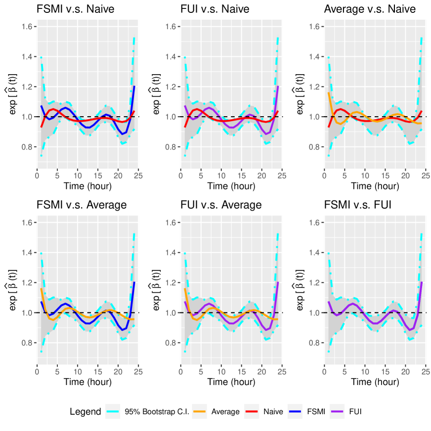
Figure 2: Plots of pairwise comparisons between FSMI, FUI, average, and naive estimates of the exponentiated coefficients of the association between step count and T2D [$\exp\{\hat{\beta}(t)\}$] after adjusting for age, sex, and race in data from the 2005-2006 NHANES. The shaded areas are the nonparametric $95\%$ point-wise bootstrap confidence intervals (CI) of [$\exp{\hat{\beta}(t)}$] with the FSMI estimator. The dashed cyan lines represent the $95\%$ point-wise lower and upper bounds of these CIs.

7 DISCUSSION

We developed the multi-level generalized functional linear regression model with functional covariates prone to heteroscedastic errors. These models are suited to massive longitudinal functional data assumed to be error-prone, such as those collected by wearable devices at frequent intervals over multiple days. Additionally, the measurement error component of the model was also developed under the multi-level generalized functional linear regression models framework. To date, most approaches to correcting measurement error in functional data analysis are based on the assumption that surrogate measures, $W_{ij}(t)$, follow Gaussian distributions. We assumed an exponential family distribution for the surrogate measures and Gaussian error processes for the measurement error. We implemented regression calibration methods to correct for measurement error and allow arbitrary heteroscedastic covariance matrices for the measurement errors. To evaluate our new methods, we conducted simulations that involved Poisson assumptions for the surrogate measures and Gaussian error processes for the measurement errors. The regression calibration methods generally had lower $\text{Abias}^{2}$ than estimators based on averaging and naive methods that do not correct for measurement error explicitly. While the average estimator reduced bias more than the naive estimator, it does not provide any formal correction of measurement error in the estimation. Likewise, the average and naive estimators produced $\text{Abias}^{2}$ values that were larger than the FSMI and FUI estimators and not statistically consistent. The FSMI estimator yielded lower $\text{Abias}^{2}$ and Avar than the FUI estimator because FSMI focuses on multiple time points concurrently in the estimation while FUI is a univariate approach. Overall, both regression calibration methods performed better than the average and naive methods with increasing sample sizes and varying levels of correlations in the serially observed functional covariate prone to errors.

We illustrated our new methods in analyses of data from the NHANES. We assessed the association between a device-based measure of step count, a surrogate for true physical activity counts, and T2D in adults in the U.S. The FSMI and FUI estimators were equivalent in our analyses and they demonstrated some correction of measurement error compared to the average and naive estimators.

8 SUPPLEMENTARY MATERIAL

None

References

- Armstrong and Bull (2006) Armstrong, Timothy and Bull, Fiona. (2006). Development of the World Health Organization Global Physical Activity Questionnaire (GPAQ). Journal of Public Health 14(2), 66–70.
- Balk and others (2015) Balk, Ethan M, Earley, Amy, Raman, Gowri, Avendano, Esther A, Pittas, Anastassios G and Remington, Patrick L. (2015). Combined diet and physical activity promotion programs to prevent type 2 diabetes among persons at increased risk: a systematic review for the community preventive services task force. Annals of Internal Medicine 163(6), 437–451.
- Bartlett and Keogh (2018) Bartlett, Jonathan W and Keogh, Ruth H. (2018). Bayesian correction for covariate measurement error: a frequentist evaluation and comparison with regression calibration. Statistical Methods in Medical Research 27(6), 1695–1708.
- Bassett (2012) Bassett, D.R. (2012). Device-based monitoring in physical activity and public health research. Physiological Measurement 33(11), 1769.
- Boyle and others (2010) Boyle, James P, Thompson, Theodore J, Gregg, Edward W, Barker, Lawrence E and Williamson, David F. (2010). Projection of the year 2050 burden of diabetes in the US adult population: dynamic modeling of incidence, mortality, and prediabetes prevalence. Population Health Metrics 8(1), 29.
- Cardot and others (2007) Cardot, H., Crambes, C., Kneip, A. and Sarda, P. (2007). Smoothing splines estimators in functional linear regression with errors-in-variables. Computational Statistics & Data Analysis 51(10), 4832–4848.
- Carroll and others (2006) Carroll, Raymond J, Ruppert, David, Stefanski, Leonard A and Crainiceanu, Ciprian M. (2006). Measurement error in nonlinear models: a modern perspective. CRC press.
- Crainiceanu and others (2009) Crainiceanu, Ciprian M, Staicu, Ana-Maria and Di, Chong-Zhi. (2009). Generalized multilevel functional regression. Journal of the American Statistical Association 104(488), 1550–1561.
- Crambes and others (2009) Crambes, Christophe, Kneip, Alois, Sarda, Pascal and others. (2009). Smoothing splines estimators for functional linear regression. The Annals of Statistics 37(1), 35–72.
- Crouter and others (2006) Crouter, S.E., Churilla, J.R. and Bassett, D.R. (2006). Estimating energy expenditure using accelerometers. European Journal of Applied Physiology 98(6), 601–612.
- Cui and others (2021) Cui, E., Leroux, A., Smirnova, E. and Crainiceanu, C.M. (2021). Fast univariate inference for longitudinal functional models. Journal of Computational and Graphical Statistics, 1–12.
- Eckel and others (2011) Eckel, Robert H, Kahn, Steven E, Ferrannini, Ele, Goldfine, Allison B, Nathan, David M, Schwartz, Michael W, Smith, Robert J and Smith, Steven R. (2011). Obesity and type 2 diabetes: what can be unified and what needs to be individualized? The Journal of Clinical Endocrinology & Metabolism 96(6), 1654–1663.
- Fearn and others (2008) Fearn, T, Hill, DC and Darby, SC. (2008). Measurement error in the explanatory variable of a binary regression: regression calibration and integrated conditional likelihood in studies of residential radon and lung cancer. Statistics in Medicine 27(12), 2159–2176.
- Freedson and others (1998) Freedson, P.S., Melanson, E. and Sirard, J. (1998). Calibration of the computer science and applications, inc. accelerometer. Medicine and Science in Sports and Exercise 30(5), 777–781.
- Gaynanova and others (2022) Gaynanova, Irina, Punjabi, Naresh and Crainiceanu, Ciprian. (2022). Modeling continuous glucose monitoring (cgm) data during sleep. Biostatistics 23(1), 223–239.
- Goldsmith and others (2011) Goldsmith, Jeff, Bobb, Jennifer, Crainiceanu, Ciprian M, Caffo, Brian and Reich, Daniel. (2011). Penalized functional regression. Journal of Computational and Graphical Statistics 20(4), 830–851.
- Jacobi and others (2007) Jacobi, D., Perrin, A.E., Grosman, N., Doré, M.F., Normand, S., Oppert, J.M. and Simon, C. (2007). Physical activity-related energy expenditure with the rt3 and tritrac accelerometers in overweight adults. Obesity 15(4), 950–956.
- Jadhav and others (2022) Jadhav, Sneha, Tekwe, Carmen D and Luan, Yuanyuan. (2022). A function-based approach to model the measurement error in wearable devices. Statistics in Medicine 41(24), 4886–4902.
- Johnson and others (2013) Johnson, Clifford L, Paulose-Ram, Ryne, Ogden, Cynthia L, Carroll, Margaret D, Kruszan-Moran, Deanna, Dohrmann, Sylvia M and Curtin, Lester R. (2013). National health and nutrition examination survey. analytic guidelines, 1999-2010.
- Kozey and others (2010) Kozey, S.L., Lyden, K., Howe, C.A., Staudenmayer, J.W. and Freedson, P.S. (2010). Accelerometer output and met values of common physical activities. Medicine and Science in Sports and Exercise 42(9), 1776.
- Kuo and others (2016) Kuo, Chih-En, Liu, Yi-Che, Chang, Da-Wei, Young, Chung-Ping, Shaw, Fu-Zen and Liang, Sheng-Fu. (2016). Development and evaluation of a wearable device for sleep quality assessment. IEEE Transactions on Biomedical Engineering 64(7), 1547–1557.
- Li and others (2007) Li, Yehua, Guolo, Annamaria, Hoffman, F Owen and Carroll, Raymond J. (2007). Shared uncertainty in measurement error problems, with application to nevada test site fallout data. Biometrics 63(4), 1226–1236.
- Pepe and Fleming (1991) Pepe, Margaret Sullivan and Fleming, Thomas R. (1991). A nonparametric method for dealing with mismeasured covariate data. Journal of the American Statistical Association 86(413), 108–113.
- Plasqui and Westerterp (2007) Plasqui, G. and Westerterp, K.R. (2007). Physical activity assessment with accelerometers: an evaluation against doubly labeled water. Obesity 15(10), 2371–2379.
- Rothney and others (2008) Rothney, M.P., Schaefer, E.V., Neumann, M.M., Choi, L. and Chen, K.Y. (2008). Validity of physical activity intensity predictions by actigraph, actical, and rt3 accelerometers. Obesity 16(8), 1946–1952.
- Sallis and Saelens (2000) Sallis, J.F. and Saelens, B.E. (2000). Assessment of physical activity by self-report: status, limitations, and future directions. Research Quarterly for Eexercise and Sport 71(sup2), 1–14.
- Silverman and Ramsay (2005) Silverman, BW and Ramsay, JO. (2005). Functional Data Analysis. Springer.
- Spiegelman and Flier (2001) Spiegelman, Bruce M and Flier, Jeffrey S. (2001). Obesity and the regulation of energy balance. Cell 104(4), 531–543.
- Spiegelman and Casella (1997) Spiegelman, Donna and Casella, Mario. (1997). Fully parametric and semi-parametric regression models for common events with covariate measurement error in main study/validation study designs. Biometrics, 395–409.
- Swartz and others (2000) Swartz, A.M., Strath, S.J., Bassett, D.R., O’Brien, W.L., King, G.A. and Ainsworth, B.E. (2000). Estimation of energy expenditure using csa accelerometers at hip and wrist sites. Medicine and Science in Sports and Exercise 32(9; SUPP/1), S450–S456.
- Tekwe and others (2019) Tekwe, C.D., Zoh, R.S., Yang, M., Carroll, R.J., Honvoh, G., Allison, D.B., Benden, M. and Xue, L. (2019). Instrumental variable approach to estimating the scalar-on-function regression model with measurement error with application to energy expenditure assessment in childhood obesity. Statistics in Medicine 38(20), 3764–3781.
- Tekwe and others (2014) Tekwe, Carmen D, Carter, Randy L, Cullings, Harry M and Carroll, Raymond J. (2014). Multiple indicators, multiple causes measurement error models. Statistics in Medicine 33(25), 4469–4481.
- Tekwe and others (2022) Tekwe, Carmen D, Zhang, Mengli, Carroll, Raymond J, Luan, Yuanyuan, Xue, Lan, Zoh, Roger S, Carter, Stephen J, Allison, David B and Geraci, Marco. (2022). Estimation of sparse functional quantile regression with measurement error: a simex approach. Biostatistics 23(4), 1218–1241.
- Troiano and others (2008) Troiano, R.P., Berrigan, D., Dodd, K.W., Masse, L.C., Tilert, T. and McDowell, M. (2008). Physical activity in the united states measured by accelerometer. Medicine and Science in Sports and Exercise 40(1), 181.
- Tsai and others (2019) Tsai, Chih-Wei, Li, Chun-Hung, Lam, Ringo Wai-Kit, Li, Chi-Kwong and Ho, Sam. (2019). Diabetes care in motion: Blood glucose estimation using wearable devices. IEEE Consumer Electronics Magazine 9(1), 30–34.
- Tuominen and others (2019) Tuominen, Jarno, Peltola, Karoliina, Saaresranta, Tarja and Valli, Katja. (2019). Sleep parameter assessment accuracy of a consumer home sleep monitoring ballistocardiograph beddit sleep tracker: a validation study. Journal of Clinical Sleep Medicine 15(3), 483–487.
- Valenti and others (2014) Valenti, G., Camps, S.G.J.A., Verhoef, S.P.M., Bonomi, A.G. and Westerterp, K.R. (2014). Validating measures of free-living physical activity in overweight and obese subjects using an accelerometer. International Journal of Obesity 38(7), 1011–1014.
- Warolin and others (2012) Warolin, Joshua, Carrico, Amanda R, Whitaker, Lauren E, Wang, Li, Chen, Kong Y, Acra, Sari and Buchowski, Maciej S. (2012). Effect of bmi on prediction of accelerometry-based energy expenditure in youth. Medicine and Science in Sports and Exercise 44(12), 2428.
- Ye and others (2008) Ye, Wen, Lin, Xihong and Taylor, Jeremy MG. (2008). Semiparametric modeling of longitudinal measurements and time-to-event data–a two-stage regression calibration approach. Biometrics 64(4), 1238–1246.
- Zoh and others (2022) Zoh, Roger S, Luan, Yuanyuan and Tekwe, Carmen. (2022). A fully Bayesian semi-parametric scalar-on-function regression (SoFR) with measurement error using instrumental variables. arXiv preprint arXiv:2202.00711.