DermSynth3D: Synthesis of in-the-wild Annotated Dermatology Images

Abstract

In recent years, deep learning (DL) has shown great potential in the field of dermatological image analysis. However, existing datasets in this domain have significant limitations, including a small number of image samples, limited disease conditions, insufficient annotations, and non-standardized image acquisitions. To address these shortcomings, we propose a novel framework called DermSynth3D. DermSynth3D blends skin disease patterns onto 3D textured meshes of human subjects using a differentiable renderer and generates 2D images from various camera viewpoints under chosen lighting conditions in diverse background scenes. Our method adheres to top-down rules that constrain the blending and rendering process to create 2D images with skin conditions that mimic in-the-wild acquisitions, ensuring more meaningful results. The framework generates photo-realistic 2D dermoscopy images and the corresponding dense annotations for semantic segmentation of the skin, skin conditions, body parts, bounding boxes around lesions, depth maps, and other 3D scene parameters, such as camera position and lighting conditions. DermSynth3D allows for the creation of custom datasets for various dermatology tasks. We demonstrate the effectiveness of data generated using DermSynth3D by training DL models on synthetic data and evaluating them on various dermatology tasks using real 2D dermatological images. We make our code publicly available at https://github.com/sfu-mial/DermSynth3D

1 Introduction

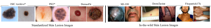
Figure 1: Standardized vs in-the-wild skin lesion images ($*$: dermoscopy, all others: clinical).

The diagnosis and analysis of skin conditions are an enormous burden on the healthcare system, with at least $3000$ distinct skin diseases identified [10] so far. Both human dermatologists and sophisticated computerized approaches struggle to address this complex task of analyzing skin conditions. Computerized analysis of skin diseases often rely on 2D colored images, with significant research efforts devoted to analysis of conditions within clinical [47] and dermoscopy images [15]. While clinical images can capture a variety of skin conditions using a common digital camera, dermoscopy images offer a more standardized acquisition using a dermatoscope, which captures a highly magnified image of the lesion with details imperceptible to the naked eye.

Dermoscopy images generally focus on the analysis of a single lesion, with large scale annotated dermoscopy datasets now available for public use [74, 20, 63]. While dermoscopy has been shown to improve the diagnostic ability of trained specialists, the field-of-view of a dermoscopy image is generally limited to a localized patch of skin on the body (e.g., a mole). In contrast, clinical images vary considerably in their acquisition protocols, ranging from a closeup view focused on a single lesion, to a view that captures a significant portion of the body (Figure 1). The contextual information in large-scale clinical images of skin lesions may provide valuable cues regarding the underlying disease that may not be present in dermoscopic images alone [63, 11].

Clinical images exhibit considerable variability across datasets. For example, the public DermoFit Image Library dataset [72, 7] contains 1300 clinical images and manual lesion segmentations from 10 types of skin conditions. These are high-quality images acquired under standardized conditions. In contrast, other clinical datasets, such as SD-198 [69], SD-260 [83], or Fitzpatrick17K [36], contain hundreds of types of skin disorders and are much less standardized, exhibiting a high variability in camera position relative to the lesion, resulting in dramatic changes in the field-of-view. We use the term “in-the-wild clinical dataset” to describe these types of image collections, where the camera position, field-of-view, and background, are inconsistent.

In-the-wild clinical images are often used to train a classification model [69, 40, 36, 82, 25], where the entire image is taken as input, and the model is trained to produce a label (e.g., class of skin disorder). However, there are several important dermatological tasks apart from classification of skin disorders, such as lesion segmentation [52, 37], lesion tracking [88, 32, 68], lesion management [3], and skin tone prediction [44]. As an example, [75] motivated their release of a public wound segmentation dataset of 2D clinical images by noting that wound segmentation may help automate the process of measuring the wound area to monitor healing and determine therapies. In addition, [34] showed that chronic wound bioprinting based on image segmentation can help facilitate wound treatments. [36] created a public dataset of 2D clinical images with skin disorder and Fitzpatrick skin tone labels [30, 31] and noted the need to segment pixels containing healthy skin when applying automated methods to estimate the skin tones of the imaged subjects. Other works [46, 53, 59, 90] have motivated the importance of considering multiple lesions over a widely imaged area, as opposed to focusing on a single lesion, noting that the presence of multiple nevi (moles) is an important indicator for melanoma [33].

One approach to curate the necessary data is to synthesize images with their corresponding annotations, which has shown success in other domains, both medical and non-medical. For example, for non-medical applications, image synthesis with annotations has been used in face analysis [81] and indoor scene segmentation [50]. For a more comprehensive review of image synthesis, particularly using generative adversarial network (GAN) models [35, 79], we direct the interested readers to the survey by [66]. Since medical image datasets tend to be small [45, 23, 6], synthesis for medical image analysis applications has also gained popularity in recent years to generate ground truth-annotated images, including but not limited to MRI [16, 26], CT [54, 19], PET [9, 78], and ultrasound [73, 49]. For a more in-depth review of the use of GANs and image synthesis in medical imaging, we refer the interested readers to comprehensive surveys by [85], [41], [76], [67], and [84].

Similarly, for skin image analysis, there have been several works towards the synthesis of skin lesion images. The first two works to explore skin lesion image synthesis used a variety of noise-based GANs [8] and conditioned the output on the diagnostic category [12]. [1] then proposed a GAN-based framework to generate skin lesion images constrained to binary lesion segmentation masks, while [57] used GANs to generate both skin lesion images as well as the corresponding binary segmentation masks.

For a more detailed review of the literature on deep learning-based synthetic data generation for skin lesion images, we refer interested readers to the comprehensive survey by [52].

While there are numerous publicly available 2D dermatological image datasets [52], existing “in-the-wild” clinical datasets have limitations in creating semantically rich ground truth (GT) labels that can be used for the diverse range of dermatological tasks discussed earlier. Consequently, compared to dermoscopic images’ synthesis, there is considerably less research in the synthetic data generation of clinical images. [48] proposed to synthesize 2D data by blending small lesions onto a larger 2D image of the torso, which allowed them to create training data for a neural network that detects lesions’ masks across a large region of the body. [24] proposed to generate burn images with automatic annotations. They used a Style-GAN [39] to synthesize burn wounds, blended the generated burns with textures from a 3D human avatar, and generated a 2D training dataset through sampling from different 2D views of the 3D avatar with the synthetic burns. Both approaches motivated their use of synthetic data by noting the difficulties in collecting appropriate real labeled training data that is specific to their dermatological task.

Our proposed work is similar to that of [24] in that we follow a similar pipeline where 2D images of the skin disorder are blended onto the 3D textured meshes and used to create a large-scale 2D dataset with corresponding annotations. However, we extend this framework by incorporating a deep blending approach to blend lesions across seams in 2D rendered views. Additionally, we broaden the scope of this work by including a diverse range of skin tones and background scenes, enabling us to generate semantically rich and meaningful labels for 2D in-the-wild clinical images that can be used for a variety of dermatological tasks, as opposed to just one. To facilitate future extensions to our framework, we have made our code base highly modular and publicly available.

⬇

from dermsynth3d import (SelectAndPaste,

BlendLesions,

Generate2DViews)

# Load settings stored in YAML file, such as:

# file paths, number of lesions to blend,

# scene parameters for the renderer, etc.

config = (...)

select_locations = SelectAndPaste(config)

select_locations.paste_on_locations()

blender = BlendLesions(config)

blender.blend_lesions()

renderer = Generate2DViews(config)

renderer.synthesize_views()

Listing 1: A minimal example of the code showing the usage of our proposed pipeline DermSynth3D, which illustrates the process of selecting a location to place the lesion on the mesh, followed by blending the lesion with the texture image, and finally rendering 2D synthetic views with corresponding labels. Infinite variations such as lighting, viewpoints, lesions, etc. can be specified in the configurations.

1.1 Contributions

Despite the availability of numerous skin image datasets  [7, 74, 40, 75, 36, 80, 25], there is a lack of a large-scale skin-image dataset that can be applied to a variety of skin analysis tasks, especially in an in-the-wild clinical setting.

To address this gap, we present DermSynth3D, a computational pipeline along with an open-source software library, for generating synthetic 2D skin image datasets using 3D human body meshes blended with skin disorders from clinical images. Our approach uses a differentiable renderer to blend the skin lesions within the texture image of the 3D human body and generates 2D views along with corresponding annotations, including semantic segmentation masks for skin conditions, healthy skin, non-skin regions, and anatomical regions. Furthermore, we demonstrate the utility of the synthesized data by using it to train machine learning models and evaluating them on real-world dermatological images, showcasing that the DermSynth3D-trained model learns to generalize to a variety of dermatological tasks. Additionally, the open-source and modular design of our framework offers opportunities for researchers in the community to experiment and choose from a range of 2D skin disorders, renderers, 3D scans, and various other scene parameters. We present a simplified code snippet in Listing LABEL:listing:code_snippet that exemplifies the modular implementation of our proposed framework and emphasizes its user-friendliness and ease of use.

Table 1: Summary of Notations

$T_{b}$

2D texture image w/ blended skin conditions

$\kappa$

Camera parameters for a 2D view

$f$

A mesh face

$F$

Set of mesh faces

$\tilde{f}$

Indices of 3D mesh faces in a 2D view

$x$

2D image

$H$

Image height

$W$

Image width

$L$

Lighting parameters for rendering

$\mathcal{M}$

Material parameters for rendering

$M$

3D mesh

$T_{\mathrm{nonskin}}$

2D texture mask of non-skin regions

$s$

2D binary segmentation mask

$H_{T}$

Texture image height

$T$

2D texture image

$T_{m}$

2D texture mask of blended skin conditions

$W_{T}$

Texture image width

$U$

Set of UV texture coordinates

$V$

Set of mesh vertices

$\tilde{a}$

2D view of a 3D mesh

$\tilde{a}_{T_{b}}$

2D view w/ blended skin condition

$\tilde{z}$

2D view w/ depth values

$\tilde{a}_{T_{d}}$

2D view w/ dilated pasted skin condition

$\tilde{H}$

2D view height

$\tilde{a}_{T_{m}}$

2D mask of the skin condition

$a_{\mathrm{nonskin}}$

2D mask of the non-skin regions

$\tilde{a}_{T}$

2D view w/ original textures

$\tilde{a}_{T_{p}}$

2D view w/ pasted skin condition

$a_{\mathrm{skin}}$

2D mask of the skin

$\tilde{W}$

2D view width

$w$

Scalar weight of the camera-to-mesh distance

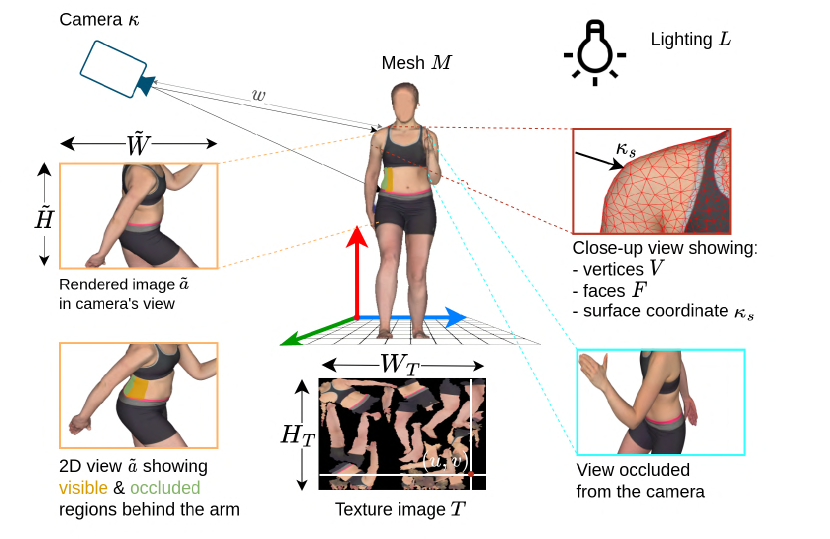
Figure 2: A figure depicting the essential notations illustrating the conditions for camera positioning, which require that the camera is positioned outside the mesh and that the mesh does not obstruct the light rays.

2 Methods

Our proposed DermSynth3D framework automates the process of blending skin disease regions from 2D images onto 3D texture meshes, while allowing for control over lighting and material parameters, from appropriate camera viewpoints, and renders the resulting 2D image and the corresponding ground truth annotations. Figure 3 shows our proposed framework. Here, we describe the rendering of a single image of a single mesh augmented with a single lesion. However, as these steps are automated, large-scale, multi-lesion datasets can be easily generated. We provide a summary of the mathematical notations used in this paper in Table 1.1 and Figure 2.

We define a 2D clinical image $\lx@glossaries@gls@link{notation}{image}{\leavevmode x}\in\mathbb{R}^{\lx@glossaries@gls@link{notation}{imageWidth}{\leavevmode W}\times\lx@glossaries@gls@link{notation}{imageHeight}{\leavevmode H}\times 3}$ as an RGB image with width $W$ and height $H$ that shows a skin condition, and a corresponding binary segmentation mask $\lx@glossaries@gls@link{notation}{segMask}{\leavevmode s}\in\{0,1\}^{\lx@glossaries@gls@link{notation}{imageWidth}{\leavevmode W}\times\lx@glossaries@gls@link{notation}{imageHeight}{\leavevmode H}}$ where pixels with a non-zero value indicate the diseased region (as shown in “2D Lesions” in Figure 3).

We define a 3D avatar of a human subject as a mesh $M$ composed of vertices $V$, faces $F$, and a UV map $U$, where the vertices and the faces determine the geometry of the mesh and the UV map determines the mapping between the geometry and a 2D texture image $\lx@glossaries@gls@link{notation}{textureImage}{\leavevmode T}\in\mathbb{R}^{W_{T}\times H_{T}\times 3}$ that contains pixels representing the surface of the skin. Our goal is to transfer the skin condition within $x$ onto a location on the texture image $T$ of the 3D mesh $M$. We approach this problem through an image-blending approach, where given a 2D binary segmentation mask $s$ indicating the skin condition within $x$ and a target location on the mesh, we blend the diseased region within the mesh’s texture image $T$.

A straightforward approach to blend a 2D image with a 3D model would be to blend $x$ directly with $T$. However, as can be seen in the “texture image” in Figure 3, this is challenging as the 2D texture image splits the human body based on seams and maps to 2D regions that are not semantically localized in 3D, which can pose a challenge for larger skin conditions that may span across seams. To address this, our proposed approach blends skin patterns on a 2D view $\tilde{a}$ of a 3D mesh rendered using a differentiable renderer, from various camera viewpoints under chosen lighting conditions. We also impose constraints to avoid blending skin patterns at unsuitable locations such as across disjoint anatomy. We describe each component of our proposed approach in detail in the following sections.

To render 2D images from meshes, we use the PyTorch3D [58] implementation of a differentiable renderer, which is composed of a rasterizer and a shader. The rasterizer determines the mesh’s faces that influence a pixel in the rendered 2D, while the shader determines the pixel value. As described by [58], the rasterizer also computes fragment data, which contains the mesh’s face identifiers, barycentric coordinates, and distances from the camera to the surface of the 3D object. In the following notation, we combine both the rasterizer and shader into a single differentiable renderer function $R(\cdot)$, which returns the rendered image as well as the fragments. Specifically, given the mesh $M$, texture image $T$, intrinsic and extrinsic camera parameters $\kappa$, lighting parameters $L$, material parameters $\mathcal{M}$, and a rendered view width ~W and height ~H, we render a 2D view $\tilde{a}$ of the 3D mesh:

$$\lx@glossaries@gls@link{notation}{view2d}{\leavevmode\tilde{a}},\lx@glossaries@gls@link{notation}{faces2d}{\leavevmode\tilde{f}},\tilde{z}=R(\lx@glossaries@gls@link{notation}{mesh}{\leavevmode M},\lx@glossaries@gls@link{notation}{textureImage}{\leavevmode T};\lx@glossaries@gls@link{notation}{cameraParameters}{\leavevmode\kappa},\lx@glossaries@gls@link{notation}{lightingParameters}{\leavevmode L},\lx@glossaries@gls@link{notation}{materialParameters}{\leavevmode\mathcal{M}},\lx@glossaries@gls@link{notation}{viewWidth}{\leavevmode\tilde{W}},\lx@glossaries@gls@link{notation}{viewHeight}{\leavevmode\tilde{H}})$$ (1)

where the rendered 2D view $\lx@glossaries@gls@link{notation}{view2d}{\leavevmode\tilde{a}}\in\mathbb{R}^{\lx@glossaries@gls@link{notation}{viewWidth}{\leavevmode\tilde{W}}\times\lx@glossaries@gls@link{notation}{viewHeight}{\leavevmode\tilde{H}}\times 3}$ has the given width and height; $\lx@glossaries@gls@link{notation}{faces2d}{\leavevmode\tilde{f}}\in\mathbb{Z}^{\lx@glossaries@gls@link{notation}{viewWidth}{\leavevmode\tilde{W}}\times\lx@glossaries@gls@link{notation}{viewHeight}{\leavevmode\tilde{H}}}$ indicates the indices of the faces of the mesh that are visible within $\tilde{a}$; $\lx@glossaries@gls@link{notation}{viewDepth2d}{\leavevmode\tilde{z}}\in\mathbb{Z}^{\lx@glossaries@gls@link{notation}{viewWidth}{\leavevmode\tilde{W}}\times\lx@glossaries@gls@link{notation}{viewHeight}{\leavevmode\tilde{H}}}$ indicates the depth of the mesh with respect to the camera position for each pixel in $\tilde{a}$; and, $R(\cdot)$ is a differentiable rendering function. The camera parameters $\kappa$ control where on the body the skin condition is to be blended and $L$ and $\mathcal{M}$ describe the lighting and material parameters respectively which jointly control the visual appearance.

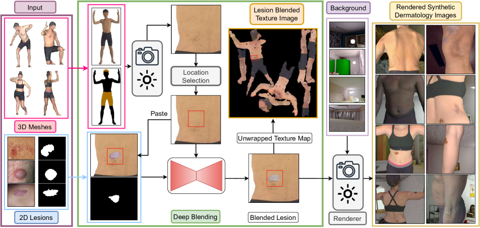
Figure 3: The DermSynth3D computational pipeline where 2D segmented skin conditions are blended into the texture image of a 3D mesh on locations outside of the hair and clothing regions. After blending, 2D views of the mesh are rendered with a variety of camera viewpoints and lighting conditions and combined with background images to create a synthetic dermatology dataset.

2.1 Determination of Skin Condition Location on the Mesh

While skin conditions can manually be placed on different potential locations on the mesh, we enforce our automated approach to place skin conditions only at suitable locations. We define the following criteria for a suitable location: the region where a lesion can be placed on the mesh, should; (1) not overlap with clothes or the hair on the head, (2) not overlap with the background, (3) have minimal depth changes, preventing blending lesions across disjoint anatomy. Specifically, as shown in Figure 2 (the 2D view $\tilde{a}$) for instance, we must avoid blending a lesion that extends across and covers both the right arm and the torso behind the right arm. Also, when blending multiple skin conditions, we ensure that skin conditions do not overlap. Accordingly, to ensure that the human anatomy remains in the camera’s field of view, we constrain the camera’s viewpoint to point to a specific coordinate $\lx@glossaries@gls@link{notation}{cameraParameters}{\leavevmode\kappa}_{s}$ on the surface of the mesh, referred to as the surface coordinate. To determine the camera’s position in the world space, we compute the weighted sum of the surface coordinate and its normal vector, where the weight is controlled by the parameter $w$. We express this operation as:

$$\lx@glossaries@gls@link{notation}{cameraParameters}{\leavevmode\kappa}_{p}=\lx@glossaries@gls@link{notation}{cameraParameters}{\leavevmode\kappa}_{s}+n(\lx@glossaries@gls@link{notation}{cameraParameters}{\leavevmode\kappa}_{s})*\lx@glossaries@gls@link{notation}{weightDistance}{\leavevmode w}$$ (2)

where $\lx@glossaries@gls@link{notation}{cameraParameters}{\leavevmode\kappa}_{p}\in\mathbb{R}^{3}$ is the camera position; $\lx@glossaries@gls@link{notation}{cameraParameters}{\leavevmode\kappa}_{s}\in\mathbb{R}^{3}$ is the surface coordinate; and $n(\lx@glossaries@gls@link{notation}{cameraParameters}{\leavevmode\kappa}_{s})$ is the normal at the surface coordinate $\lx@glossaries@gls@link{notation}{cameraParameters}{\leavevmode\kappa}_{s}$. The scalar weight $w$ controls the distance from the camera to the surface of the mesh, where a larger weight places the camera further from the surface, i.e., captures a larger field of view. Sampling the weights $w$ and surface coordinates $\lx@glossaries@gls@link{notation}{cameraParameters}{\leavevmode\kappa}_{s}$ results in a range of views; however, many views are unsuitable to place the skin condition.

Thus, first, we check the suitability of placing a scaled clinical image $x$ and lesion mask $s$ (scaled as $x$ and $\tilde{a}$ can be different sizes) at the center of the rendered view, by first composing an image $a_{x}\in\mathbb{R}^{\lx@glossaries@gls@link{notation}{viewWidth}{\leavevmode\tilde{W}}\times\lx@glossaries@gls@link{notation}{viewHeight}{\leavevmode\tilde{H}}\times 3}$ (showing the lesion on the rendered view) and a corresponding lesion mask $a_{s}\in\mathbb{R}^{\lx@glossaries@gls@link{notation}{viewWidth}{\leavevmode\tilde{W}}\times\lx@glossaries@gls@link{notation}{viewHeight}{\leavevmode\tilde{H}}}$. We then check if the region $a_{s}$, where the skin disorder was placed meets the aforementioned criteria. For ensuring minimal depth changes and avoiding lesion overlap with the background, we rely on the depth $\tilde{z}$ from the renderer (Eq. 1) to avoid local regions that have a high depth change or are outside the mesh. Moreover, to avoid lesion overlap with non-skin regions, we use manual annotations (Section 3.1) of non-skin regions on the texture image to distinguish skin from non-skin regions. Further details are supplied in A.

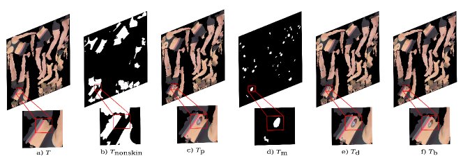
Figure 4: The different variants of texture images produced by DermSynth3D with a corresponding close view of skin -conditions. Left to right: Original texture image $T$, Binary mask indicating the non-skin regions $T_{\mathrm{nonskin}}$, texture image with the “pasted” skin conditions $T_{p}$, a mask of the texture image showing the localizations of the pasted skin -conditions $T_{m}$, a texture image $T_{d}$ created by dilating the masked lesion $s$, a texture image $T_{b}$ with the “blended” skin conditions.

2.2 Blending Skin Conditions into a Mesh’s Texture Map

Skin conditions can appear in different locations on the body and they can be captured in various views in real-world clinical settings. Thus, in order to efficiently synthesize realistic “in-the-wild” clinical images from different 3D viewpoints, our approach blends the skin disorder within the mesh’s texture image, which allows the framework to render the blended skin disorder from a varierty of views. In order for the blending to be robust to different viewpoints, we perturb the camera position during the blending process using a pasted texture image $T_{p}$ containing the original skin conditions “pasted” within the texture image. Specifically, given the regions that capture a skin condition within the view $a_{x}$ and the corresponding mask $a_{s}$, we map the masked pixels containing the skin disorder to the pixels within the texture image in order to “paste” the original segmented skin condition onto the texture image $T$. This mapping is achieved by determining the UV or texture coordinates of a vertex on the surface of the mesh corresponding to its Cartesian coordinate in the texture image.

Given a texture image (Figure 4-a), a skin mask (Figure 4-b), and an image of a skin condition and its mask (Figure 3- 2D Lesion, lower-left), our goal is to update the texture image to include a skin condition. We denote this updated texture image with the pasted skin conditions as $T_{p}$ (Figure 4-c). Following the same procedure, we create a texture image mask $T_{m}$ (Figure 4-d) that localizes the pasted skin condition, where instead of assigning the pixel value, we assign a unique integer to identify each lesion. We create an additional texture image $T_{d}$ (Figure 4-e), which is based on dilating the masked lesion $s$ to include the surrounding skin. We define $T_{b}$ (Figure 4-f) as the texture image that will be optimized during blending and is initialized with $T_{p}$. By replacing the input texture image $T$ in Eq. 1 with $T_{p}$, $T_{m}$, $T_{d}$, and $T_{b}$, we can render 2D views of the original unmodified textures ($\tilde{a}_{T}$), the pasted skin condition ($\tilde{a}_{T_{p}}$), a mask of the pasted skin condition ($\tilde{a}_{T_{m}}$), a 2D view of the dilated skin condition ($\tilde{a}_{T_{d}}$), and a 2D view of the blended skin condition ($\tilde{a}_{T_{b}}$), while keeping the camera parameters unchanged.

To create a 2D blended image, we follow the deep image blending approach by [89], where an iterative optimization, minimizes a blending loss function between a foreground object cropped from the source image and the target image which the selected object would be blended onto. We use this approach to create the 2D blended image $b$ by combining the non-dilated masked pixels $\tilde{a}_{T_{m}}$ of the lesion in the blended view $\tilde{a}_{T_{b}}$ with the non-masked pixels containing original textures $\tilde{a}_{T}$,

$$b=\lx@glossaries@gls@link{notation}{view2d}{\leavevmode\tilde{a}}_{T_{m}}\odot\lx@glossaries@gls@link{notation}{view2d}{\leavevmode\tilde{a}}_{T_{b}}+(1-\lx@glossaries@gls@link{notation}{view2d}{\leavevmode\tilde{a}}_{T_{m}})\odot\lx@glossaries@gls@link{notation}{view2d}{\leavevmode\tilde{a}}_{T},$$ (3)

where $\odot$ represents element-wise (Hadamard) multiplication. This masking causes only the pixels within the masked region to be modified while preserving the original non-masked regions.

However, in contrast to [89], instead of directly blending a 2D image, we optimize the pixels within a texture image $T_{b}$ by minimizing the blending loss using the 2D view,

$$\lx@glossaries@gls@link{notation}{blendedTextureImage}{\leavevmode T_{b}}^{*}=\operatorname*{argmin}_{{\lx@glossaries@gls@link{notation}{textureImage}{\leavevmode T}_{b}}}\mathcal{L}\left(b,\lx@glossaries@gls@link{notation}{viewBlend2d}{\leavevmode\tilde{a}_{T_{b}}},\lx@glossaries@gls@link{notation}{viewOriginal2d}{\leavevmode\tilde{a}_{T}},\lx@glossaries@gls@link{notation}{viewPaste2d}{\leavevmode\tilde{a}_{T_{p}}},\lx@glossaries@gls@link{notation}{viewDilated2d}{\leavevmode\tilde{a}_{T_{d}}},\lx@glossaries@gls@link{notation}{viewMask2d}{\leavevmode\tilde{a}_{T_{m}}}\right),$$ (4)

where $\lx@glossaries@gls@link{notation}{blendedTextureImage}{\leavevmode T_{b}}^{*}$ is the resulting texture image with the blended lesions after optimization; and, $\mathcal{L}(\cdot)$ denotes the blending loss.

We adopt the content $\mathcal{L}_{c}$, style $\mathcal{L}_{s}$, gradient $\mathcal{L}_{\nabla}$, and total variation $\mathcal{L}_{\mathrm{TV}}$ loss functions for image blending as described by [89],

$$\begin{split}\mathcal{L}=&\ \lambda_{c}\mathcal{L}_{c}(b,\lx@glossaries@gls@link{notation}{view2d}{\leavevmode\tilde{a}}_{T_{p}};\lx@glossaries@gls@link{notation}{view2d}{\leavevmode\tilde{a}}_{T_{m}})\\ &+\lambda_{s}\mathcal{L}_{s}(b,\lx@glossaries@gls@link{notation}{view2d}{\leavevmode\tilde{a}}_{T};\lx@glossaries@gls@link{notation}{view2d}{\leavevmode\tilde{a}}_{T_{m}})\\ &+\lambda_{\nabla}\mathcal{L}_{\nabla}(b,\lx@glossaries@gls@link{notation}{viewOriginal2d}{\leavevmode\tilde{a}_{T}},\lx@glossaries@gls@link{notation}{viewDilated2d}{\leavevmode\tilde{a}_{T_{d}}};\lx@glossaries@gls@link{notation}{viewMask2d}{\leavevmode\tilde{a}_{T_{m}}})\\ &+\lambda_{\mathrm{TV}}\mathcal{L}_{\mathrm{TV}}(b;\lx@glossaries@gls@link{notation}{viewMask2d}{\leavevmode\tilde{a}_{T_{m}}}),\end{split}$$ (5)

where $\mathcal{L}_{c}(\cdot)$ encourages similar CNN features between the blended and pasted view; $\mathcal{L}_{s}(\cdot)$ encourages similar styles between the blended and original textures; $\mathcal{L}_{\nabla}(\cdot)$ encourages similar gradients between the blended view and the dilated view combined (using the mask) with the gradients of the original textures; and $\mathcal{L}_{\mathrm{TV}}(\cdot)$ encourages a lower variation among neighboring pixels. The user can control the visual appearance of the blended skin conditions by modifying the weights for each related loss term, i.e., $\lambda_{c}$, $\lambda_{s}$, $\lambda_{\nabla}$, and $\lambda_{TV}$. Since only the areas within the masks are changed during the optimization, we use $\tilde{a}_{T_{m}}$ to compute a padded bounding box around the skin condition and compute the loss only over this region.

Finally, we perform an iterative optimization to minimize Eq. 4. At each step of the optimization, we add a small random value to $w$ in Eq. 2, perturbing the camera viewpoint, which helps ensure that the blended image is robust to different camera viewpoints. We highlight that the loss function $\mathcal{L}(\cdot)$ measures the quality of the blending using the 2D views, while we optimize the underlying texture image $T_{b}$. Using a differentiable renderer (Eq. 1), we can calculate the gradients with respect to the pixel values of the underlying texture image, which enables the backpropagation of the loss gradients to optimize for the pixel value adjustments.

2.3 Creating the 2D Image Dataset

Creating the dataset of 2D rendered images and corresponding dense annotations involves two steps. First, we determine an appropriate location for blending (Section 2.1) and blend the selected skin conditions (Section 2.2) onto the texture image $T$ of the 3D mesh $M$. We sample a 2D image $x$ with skin condition from a set of real dermatological images (Section 3.1) along with an annotated mask $s$. We apply the Shades of Gray algorithm [29] to improve the color constancy within $x$. We repeat the process described in Section 2.1 and Section 2.2 to blend $k$ skin conditions at different locations. The output of this first step produces a blended texture image $\lx@glossaries@gls@link{notation}{blendedTextureImage}{\leavevmode T_{b}}\in\mathbb{R}^{\lx@glossaries@gls@link{notation}{textureWidth}{\leavevmode W_{T}}\times\lx@glossaries@gls@link{notation}{textureHeight}{\leavevmode H_{T}}\times 3}$ and a corresponding texture mask $\lx@glossaries@gls@link{notation}{textureMask}{\leavevmode T_{m}}\in\mathbb{Z}^{\lx@glossaries@gls@link{notation}{textureWidth}{\leavevmode W_{T}}\times\lx@glossaries@gls@link{notation}{textureHeight}{\leavevmode H_{T}}}$ indicating the locations of the skin conditions, where WT and HT are the width and the height of the original texture image $T$ respectively. Therefore, now we have a 3D mesh with a blended lesion.

Second, we use the blended texture image $T_{b}$ and texture mask $T_{m}$ to create a dataset of rendered 2D views and corresponding target labels. To choose the camera position and direction, we use the same procedure in Eq. 2 where we randomly sample a surface coordinate $\lx@glossaries@gls@link{notation}{cameraParameters}{\leavevmode\kappa}_{s}$ on the mesh. We use Eq. 1 with the blended texture image $T_{b}$ to render a 2D RGB view $\lx@glossaries@gls@link{notation}{viewBlend2d}{\leavevmode\tilde{a}_{T_{b}}}\in\mathbb{R}^{\lx@glossaries@gls@link{notation}{viewWidth}{\leavevmode\tilde{W}}\times\lx@glossaries@gls@link{notation}{viewHeight}{\leavevmode\tilde{H}}\times 3}$ and randomly sample from a range of diffuse, ambient, and specular lighting parameters and lighting positions to introduce variations in the rendered 2D views. Moreover, for more realistic views and improved illumination, we enforce that the camera is placed outside of the mesh and that the light source reaches the camera without being blocked by the mesh. To create the final image, we combine the foreground with a background image of 2D indoor scene.

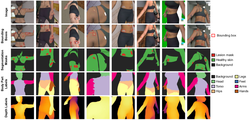
Figure 5: A few examples of data synthesized using DermSynth3D. The rows from top to bottom show respectively: the rendered images with blended skin conditions, bounding boxes around the lesions, GT semantic segmentation masks, grouped anatomical labels, and the monocular depth maps produced by the renderer.

Next, we describe each of our different target variables. When rendering binary masks in Eq. 1, we only use ambient lighting, as ambient light provides a uniform level of illumination to all parts of the object and preserves the underlying pixel values in the texture masks. The skin condition mask $\tilde{a}_{T_{m}}$ is computed by rendering with the texture mask $T_{m}$. The skin mask $a_{\mathrm{skin}}$ is computed by excluding both the skin condition regions $\tilde{a}_{T_{m}}$ and the regions of the body labeled as non-skin (computed via the rendered view using the non-skin texture mask $T_{\mathrm{nonskin}}$ as described in Section 3.1). The non-skin mask $a_{\mathrm{nonskin}}$ is computed from regions containing neither skin $\tilde{a}_{T_{m}}$ nor skin conditions $a_{\mathrm{skin}}$ (Figure 5, third row). Additionally, we obtained bounding boxes around skin condition regions by computing the minimal enclosing box around each skin condition mask (Figure 5, second row from the top).

In addition to the skin lesion segmentation masks, we create other ground truth annotations, such as body part labels and depth maps. For the body part labels, we include dense anatomical labels for 16 regions of the body (e.g., head, torso) where we use the mesh’s faces $\tilde{f}$ (from Eq. 1) visible in the rendered view $\tilde{a}_{T_{b}}$ to determine an anatomy label for each pixel in the rendered view (Section 3.2 describes how a mesh is assigned anatomical labels) and assign a background label to pixels outside the mesh (Figure 5, fourth row from the top). For the depth maps, the depth image $\tilde{z}$ is obtained from the fragments computed by the renderer (Figure 5, bottom row).

Finally, we generate our dataset by rendering a set of 2D images and the corresponding annotations for each mesh, by sampling $n$ times under different camera, lighting, and material parameters, and background scenes. We show some example images from the generated 2D dataset in Figure 6.

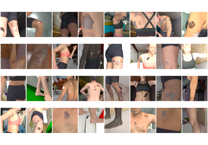
Figure 6: Generated synthetic images of multiple subjects across a range of skin tones in various skin conditions, backgrounds, lighting, and viewpoints.

The modular design of our DermSynth3D pipeline not only allows us to easily modify the aforementioned settings, but also allows us to achieve photo-realistic rendering by replacing the differential renderer $R(\cdot)$ with any physically based rendering (PBR) method such as Unity3D However, for all the experiments reported in the paper, we use PyTorch3D [58] owing to its simplicity and wide adoption in the research community. We show some qualitative samples obtained using these two kinds of renderers in Figure 7. We observe that regardless of the choice of the renderer used in creating the 2D dataset of rendered images, the downstream task of foot ulcer wound segmentation achieved almost similar quantitative performance, as shown in Figure LABEL:fig:renderSeg.

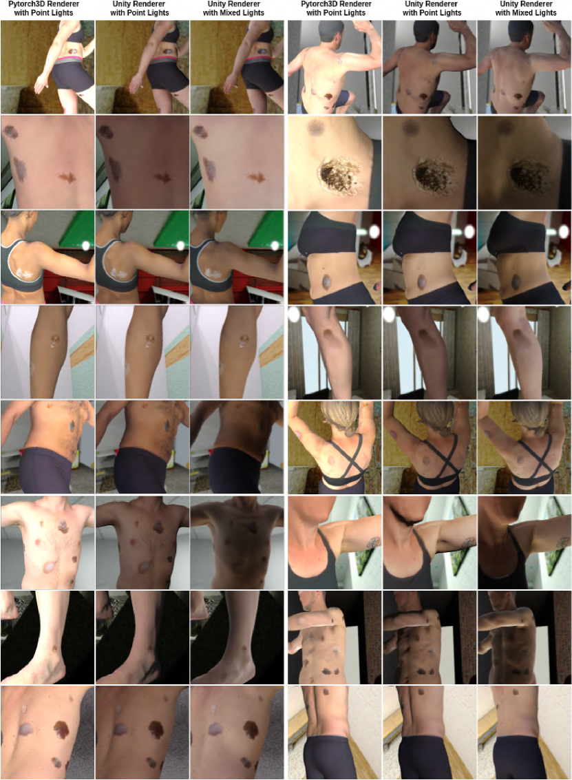
Figure 7: Some samples of the 2D images generated using PyTorch3D [58], and Unity3D renderer. We show the rendered images from Unity3D in two lighting conditions, namely Point Lights and a mix of Point and Direction Lights. For the experiments reported in the paper, we use PyTorch3D with Point Lights since it mimics the natural behavior of light in the real world.

3 Materials: Datasets and Annotations

3.1 3D Textured Human Meshes and Their Annotation

We use the 3DBodyTex [64, 65] dataset, which provides 400 high-resolution textured meshes from 200 unique subjects, each imaged in two different poses. Subjects wear sports clothing, which results in a significant amount of skin regions being exposed and captured. We manually annotate non-skin regions within the 2D texture image to create a non-skin texture mask $T_{\mathrm{nonskin}}$, which we define as regions containing clothing, hair, jewelry, etc. We select a subset of 50 annotated meshes to perform blending, where meshes are chosen to cover a wider range of skin tones available within 3DBodyTex. We provide further details in LABEL:sup:sec:annotate_nonskin.

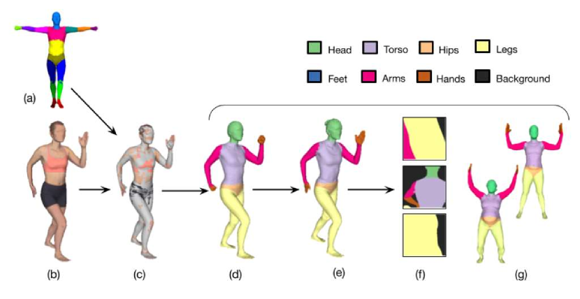
Figure 8: Proposed schema for anatomical part labeling showing: (a) 3D SCAPE template body model with $16$ anatomical part labels, (b) Input 3DBodyTex scan, (c) Template model fitted to input scan, (d) Anatomical body part labels (only 7 instead of 16, as per [27]) assigned to fitted model, (e) Anatomical labels transferred to the input scan, (f) 2D views of annotated samples, (g) More examples.

3.2 Anatomy Labels for 3DBodyTex

We segment the 3D body mesh $M$ into different anatomical parts by fitting the SCAPE body model [4] with $16$ anatomical parts annotated per-vertex onto $M$ using an automatic fitting method described by [65]. This yields a fitted mesh with the same topology and geometry as the body model, thus inheriting the body part annotations. As the fitted mesh has the same shape and pose as $M$, we can transfer the body part annotations using the nearest vertex assignment between the fitted mesh and $M$.

In Figure 8, we show the process of labeling given an input 3D body scan and a SCAPE [5] template body model. Initially, the body model comes with 16 anatomical labels consisting of: head, upper torso, lower torso, hips, upper leg left, upper leg right, lower leg left, lower leg right, feet left, feet right, upper arm left, upper arm right, lower arm left, lower arm right, hand left, hand right. For simplicity and a fair comparison with [27, 18], only 7 anatomical labels are kept namely: head, torso, hips, legs, feet, arms, and hands (Figure 8-(g)).

3.3 Segmentation of 2D Dermatological Images

We use the Fitzpatrick17K dataset [36], a clinical dataset composed of 2D “in-the-wild” clinical images and corresponding disease labels. We manually segment a total of $75$ images into lesion, skin, and background segmentations, where 50 images were used for blending and as a validation set during training, and 25 images were held out for evaluation. We point the readers to LABEL:sup:sec:annotate_fitz for more details.

3.4 Backgrounds for Synthetic Images

In the final step of generating synthetic images, we combine the foreground with a background image. Since real-world clinical settings are usually indoor environments, for generating 2D “in-the-wild” clinical images, we randomly choose the background from publicly available 2D indoor scene images [50, 61].

4 Implementation Details

4.1 Dataset Construction Details

4.1.1 Placing and Blending the Skin Condition into a Mesh

For the rendering in Eq. 1, we set the rendered width $\tilde{W}$ and height $\tilde{H}$ to $512\times 512$, and set the lighting parameters $L$ to use only point lights, placed at the same position as the camera, to avoid interference from shadows.

During the blending stage, the RGB components of ambient, specular, and diffused colors of the lighting parameters are set to $0.5$, $0.025$, and $0.5$ each, respectively. We also fix the specular color and shininess of the material to be $0.025$ and $50$, respectively. These values determine the intensity of luster and the color of the reflected light from the material, i.e., the texture image. Additionally, we use perspective projection-based cameras and set the field-of-view (FOV) as $30\degree$.

To determine the surface coordinate $\lx@glossaries@gls@link{notation}{cameraParameters}{\leavevmode\kappa}_{s}$ in Eq. 2, we explored using the center of a sampled mesh face $f$ and sampling points on the surface of the face and found minimal differences. However, this is likely dataset dependent, where meshes with coarse non-uniform faces benefit more from sampling surface points with a probability proportional to the area of the face. We set $w$ to a random value in the range [0.4, 0.6], which is a dataset-dependent range we empirically set that contributes to the scale of the blended lesion. When placing multiple skin conditions into a single texture image, we apply random horizontal and vertical flips and rotations to the lesions to introduce variability in the orientation of the lesion, where the texture mask keeps track of where the skin condition is blended to prevent skin conditions from overlapping.

To minimize Eq. 4, we use the Adam optimizer [43] with a learning rate of $0.005$ and optimize for $400$ steps per location. In Eq. 5, we set weights for each loss function as $\lambda_{c}=2$, $\lambda_{s}=10^{6}$, $\lambda_{\nabla}=10^{5}$, and $\lambda_{\mathrm{TV}}=10^{-4}$, which are set empirically to blend the lesions into the textures while preserving many of the lesions’ visual characteristics.

4.1.2 Rendering 2D Views and Creating the Dataset

We fix all rendered blended views to a height $\tilde{H}$ and width $\tilde{W}$ of $512\times 512$. We sample from a range of camera views and lighting parameters, where the ranges are empirically set to span across a variety of plausible “in-the-wild” acquisition scenarios. We sample $w$ between [0.1, 1.3] to give a range of closeup and full body field-of-views. To introduce a variety of lighting conditions while creating the 2D dataset, we sample the RGB components of ambient and diffused colors in lights from a range of [0.2, 0.99], whereas the specular color is sampled between [0, 0.1]. Furthermore, the specular color and shininess of the material is sampled between a range of [0, 0.05] and [30, 60], respectively.

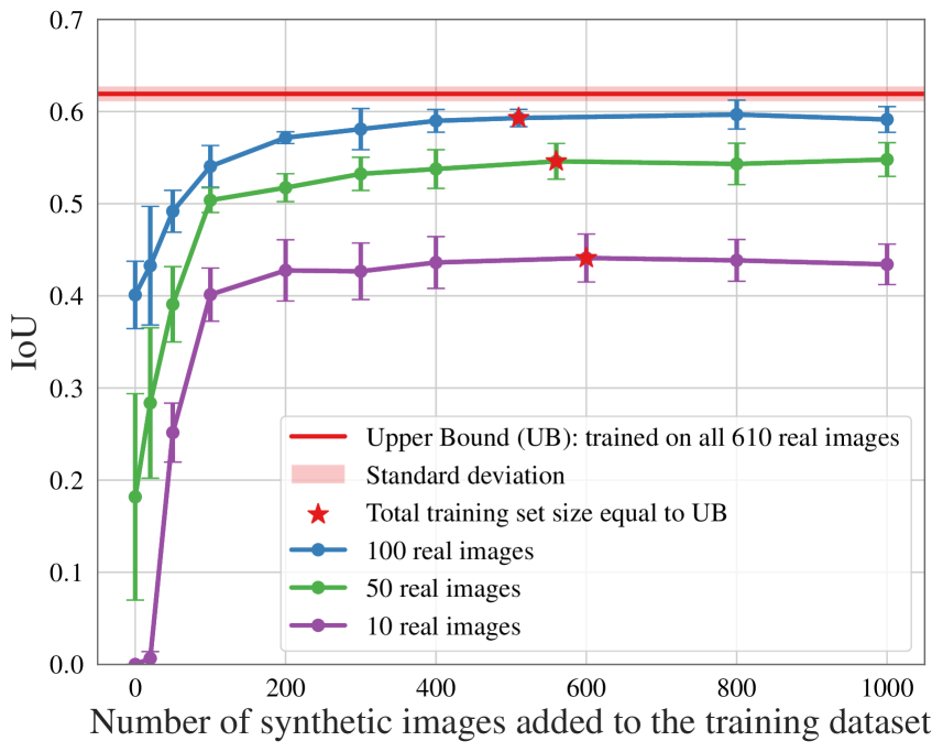
(a)

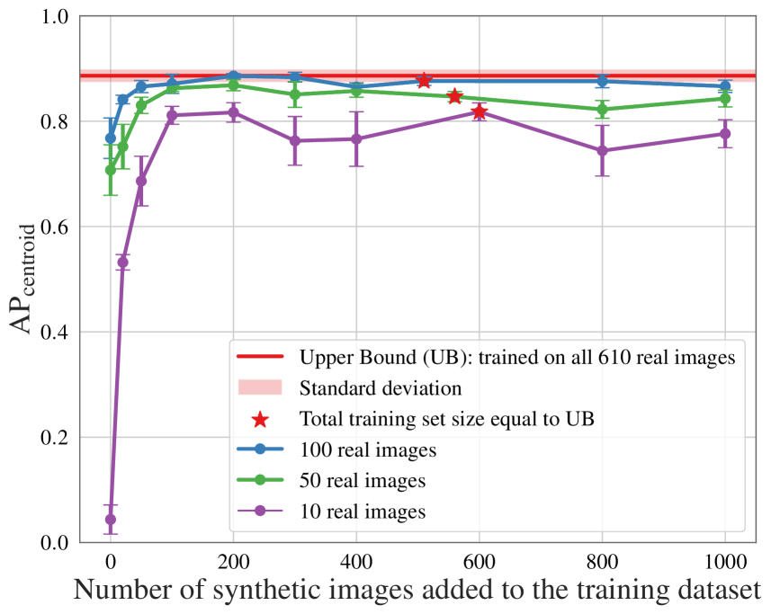
(b)

Figure 9: Wound bounding box detection performance across five folds (mean and standard deviation) on FUSeg dataset, where the number of synthetic images added to a fixed number of real images in the training set gradually increases. Bounding box detection performance is measured by (a) IoU and (b) $\mathrm{AP}_{\mathrm{centroid}}$ (note that the vertical scales of the two plots are different). The horizontal red line indicates the results for the model that is trained on 610 real images (the full-size available training set), which is considered as the upper bound performance on this dataset.

4.2 Experimental Details

4.2.1 Wound Bounding Box Detection and Semantic Segmentation in Clinical Images

We use the FUSeg dataset from the The Foot Ulcer Segmentation Challenge [75], which contains 2D clinical dermatological images of ulcers on the foot and the corresponding wound masks. The FUSeg dataset contains the standard training, validation, and testing partitions of 810, 200, and 200 images, respectively. As the ground truth annotations for the official test set are not publicly released, we use the official validation set for our evaluation and split the official training set into 610 images for training and 200 images for internal validation.

For the wound detection task, we convert the masks of the wounds to bounding boxes by labeling the connected regions of the masks and computing the minimal enclosing bounding box, and train a Faster R-CNN [60] model for bounding box detection. We use a mini-batch size of 8 images and train the model for a maximum of 50 epochs using SGD [62, 42, 13] with a learning rate of $0.001$. We choose the model weights with the maximum intersection over union (IoU) score over the internal validation set of real images.

For the wound segmentation task, we train a DeepLabV3 [17] network with a ResNet-50 [38] backbone as our model. We use a mini-batch size of 8 images and minimize the binary cross entropy loss for a maximum of 250 epochs using the Adam optimizer with a learning rate of $0.00005$ and a weight decay of $0.00005$. We choose the model weights with the maximum Dice score over the internal validation set of real images.

4.2.2 Lesions, Skin, and Background Segmentation Using In-the-wild Clinical Images

For this experiment, we train a DeepLabV3 ResNet50 [17] CNN model for a maximum of 3,430 steps, using a batch size of 8. We train on 13,720 synthetic images while validating using 50 real 2D dermatological images, and use a modified fuzzy Jaccard index [22] as the loss function. See LABEL:sup:sec:lesion_skin_bg for more details on the loss and the training procedure. We choose a model that produces the lowest Jaccard loss on our validation set consisting of 50 real 2D dermatological images that we manually segmented into regions for skin conditions, healthy skin, and non-skin. The CNN training process on this task took around one hour on an NVIDIA GeForce RTX 2070 Super 8 GB GPU, while generating the synthetic image dataset after blending took approximately three hours. Creating the dataset with 50 meshes, each with 50 skin conditions blended onto them, took around 30 hours on a Quadro-RTX-4000 8GB GPU. It is worth noting that the majority of the computing time was spent on blending the lesions to generate the dataset.

4.2.3 Lesion and Skin Segmentation on Dermoscopy, Clinical, and Non-Medical Images

In Section 5.3, we describe experiments using the dermoscopy dataset PH2 [51, 28]; the clinical dataset DermoFit [7]; and the non-medical skin dataset Pratheepan [86, 70]. We pre-process these images by applying the Shades of Gray [29] color constancy algorithm followed by image normalization (i.e., subtract image pixels by the pretrained dataset channel mean and divide by the channel standard deviation). Images are resized to maintain their aspect ratio such that the smallest spatial dimension is equal to the spatial dimension of the resized training images (320 pixels), expect for the dermoscopy dataset PH2, which is resized based on the longest spatial dimension (PH2 contains dermoscopy images, which show dermoscopic structures not visible to the naked eye and these types of images were not part of the training data). We apply Gaussian smoothing to the PH2 and DermoFit images as these images show a close-up view of the lesion with details that may not be visible in our training data.

5 Experiments and Results

We train deep learning models with pre-trained weights for bounding box detection and semantic segmentation on our synthetic data using common image augmentation and normalization techniques (e.g., rotation, color shifts), and evaluate on real 2D images including dermatological images with skin conditions. We perform these experiments in order to evaluate how well a model trained on our generated synthetic data can generalize to unseen real data. We emphasize that our goal in these experiments is not to compete with state-of-the-art performance over these datasets, but rather to show the utility of the generated dataset by assessing the model’s ability to generalize to real 2D images when trained on this dataset. Ideally, we would evaluate our approach over an existing “in-the-wild” clinical dermatological dataset with skin conditions, skin, and background segmentation labels. However, to the best of our knowledge, there exists no such dataset, as most skin image datasets contain labels for binary segmentation tasks (e.g., skin vs background or lesion vs background). Thus, we evaluate using data we manually annotated over an “in-the-wild” clinical dataset containing skin conditions, skin, and background masks, as well as over different binary segmentation tasks on prior datasets.

5.1 Wound Bounding Box Detection and Semantic Segmentation in Clinical Images

Detecting wounds in clinical images is an important step to track and extract morphological features from the wounds, which is crucial for diagnosis and treatment. Bounding boxes can be used to localize the wounds in clinical images and minimize unnecessary information within the scene to improve downstream tasks [75].

For evaluating the bounding box detection performance, we use two metrics: the intersection over union (IoU) score, which measures the exact match between a detected and ground truth bounding box, and the average precision of overlapping centroids ($\mathrm{AP}_{\mathrm{centroid}}$) [90], which determines the bounding box localization performance, rather than its precise boundaries and is more suitable for medical applications.

To assess the performance improvement from using synthetic images in the training process, we gradually increase the number of synthetic images added to the training sets of limited real images. We can see in Figure 9 that the addition of synthetic images consistently improves the detection performance and reduces the standard deviation error in the results, thus leading to more robust and reliable performance. Moreover, using only less than $\frac{1}{6}$^th of the available real images (100 annotated real images) alongside synthetic ones, we can achieve comparable detection results to the upper bound, which is less than a $2\%$ drop in performance. Note that for generating synthetic training images using DermSynth3D, only 50 lesion annotations were used, which is $8.2\%$ of the cost of dense annotations compared with the real dataset of wounds. Another notable observation in Figure 9 is that by adding 100 synthetic images to a very small dataset of 10 real images, we can achieve a similar performance as a dataset of 100 real images. This demonstrates the usefulness of this approach in situations where real data is extremely limited.

To further explore the usefulness of our synthetic images in scenarios where there is no real training data available, we conduct additional experiments. We create a synthetic dataset of 610 images, which is the same size as the “real” wound image training set of the FUSeg dataset. We then evaluate the performance of a model in bounding box detection and segmentation when it is trained on this synthetic-only dataset and tested on the real wound image testset.

The quantitative results are reported in Table 2 alongside the model’s performance when trained on the FUSeg training set of real wound images, under the same training settings.

Our experiments show that for wound detection, when only synthetic DermSynth3D data is available, an average precision of $80\%$ in wound localization can still be achieved. Additionally, for the segmentation performance, a model trained on only synthetic images still achieves a Dice score of $0.49$, which is more than $60\%$ of the performance on real data ($0.81$ Dice), despite the differences in semantic content (skin conditions selected from Fitzpatrick17K dataset versus foot ulcers) and source domains (synthetic versus real). This demonstrates that even in the absence of real images, training on synthetic DermSynth3D data can provide more than $60\%$ of the expected performance when trained on real clinical images, despite the significant domain gaps.

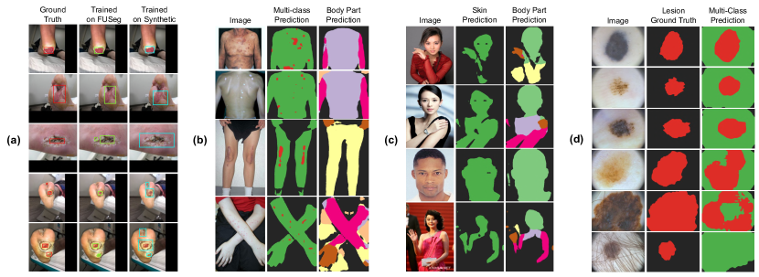
Figure 10: Qualitative results for (a) foot ulcer bounding box detection on FUSeg dataset, (b) multi-class segmentation (lesions, skin, and background) and in-the-wild body part prediction, (c) skin segmentation and body part prediction on Pratheepan dataset, and (d) multi-class segmentation (lesions, skin, and background) on dermoscopy images from PH2 dataset. The color legend is the same as Figure 5.

Table 2: Foot ulcer bounding box detection and segmentation performance on the test set of real images of wounds.

	Detection (bounding box overlap)		Segmentation (pixel-wise comparison)
Train dataset	$\mathrm{AP}_{\mathrm{centroid}}$	IoU	Dice	IoU
Synthetic	0.80 $\pm 0.018$	0.42 $\pm 0.011$	0.49 $\pm 0.007$	0.37 $\pm 0.008$
FUSeg	0.88 $\pm 0.012$	0.61 $\pm 0.008$	0.81 $\pm 0.003$	0.71 $\pm 0.004$

5.2 Lesions, Skin, and Background Segmentation Using in-the-wild Clinical Images

For our subsequent experiments, we modify the DeepLabV3 ResNet50 [17] CNN model to perform two semantic segmentation tasks: skin condition vs healthy skin vs non-skin segmentation; and anatomical semantic segmentation (Section 3.2). We add a total of 11 output channels for semantic segmentation, where three channels are used to predict the pixels containing skin conditions, healthy skin, and non-skin regions, and the remaining eight channels predict the anatomical labels. Rather than use the full 16 anatomical labels provided as per SCAPE body model [4], we follow the PASCAL-part convention [18] similar to [27] and group the semantically similar anatomical labels into a single label (e.g., “left upper arm” and “right lower arm” are given the label “arm”) as shown in Figure 8-(g).

We evaluate our approach on our manually annotated images taken from Fitzpatrick17K, an “in-the-wild” clinical 2D image dataset, where we use a subset of 25 images that were neither used for blending nor during model validation. We use our CNN model trained on synthetic data and evaluate the performance on these real images. We tested on these 25 manually segmented images and calculated the per-image Jaccard index for skin condition, skin, and non-skin segmentation. The averaged results were $0.61\pm 0.23$, $0.88\pm 0.10$, and $0.60\pm 0.43$, respectively. We show the qualitative results in Figure 10. These results suggest that the model is capable of generalizing from our synthetic data to real images.

5.3 Lesion and Skin Segmentation on Dermoscopy, Clinical, and Non-Medical Images

To further show the generalization capability of our approach, we use the same trained model described in Section 5.2 and evaluate over PH2 [51, 28], a dermoscopy dataset with 200 images; DermoFit [7], a clinical dataset of 1300 images; and the Pratheepan [86, 70] non-medical image dataset that provides manually segmented skin masks. Interestingly, we find that our model, trained on synthetic data simulating “in-the-wild” clinical images, does show the ability to generalize to these other types of datasets. When segmenting lesions from the dermoscopy PH2 dataset, we achieve a Jaccard index of $0.62\pm 0.21$ averaged over each image. For context, previous work by [2] noted that applying transfer learning from curated real clinical images of close-up views achieves slightly better performance (Jaccard index of $0.69$). When segmenting lesions from the clinical DermoFit dataset, we achieve a Jaccard index of $0.57\pm 0.21$. On the non-medical Pratheepan dataset, we use the 32 images in the “FacePhoto” partition, which shows a single closeup of a human subject, and achieve a Jaccard index of $0.76\pm 0.14$. For context, we report an F1-score of 0.86 while prior work [14] reported $0.74$. While these do not represent state-of-the-art results on these datasets, we emphasize that the purpose of these experiments is to show that our proposed approach to generate synthetic data results is of sufficient quality that a model can learn to generalize to real images. We highlight that this single model trained on the synthetic labels predicts dense semantic segmentations for both the skin task and the anatomy task, and show the qualitative results of our model predicting other types of tasks in Figure 10 (b)-(d).

5.4 Predicting Body Parts from 2D Images

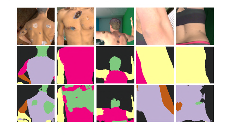
Figure 11: Qualitative results obtained by applying an existing human parsing method [27] on the proposed dataset. Top: RGB images. Middle: ground-truth anatomical labels. Bottom: predicted anatomical labels.

Understanding where the skin condition is on the body may be an important factor in determining likely skin conditions [21, 56, 87] (e.g., ruling out a diagnosis of a foot ulcer if the condition appears on the torso). While semantic segmentation of the human body, commonly referred to as human parsing, is a well-studied area, we are specifically interested in partial-body views. Existing approaches [55, 27, 77] mainly consider constrained scenarios where the human body is fully visible in the images, but performance drops considerably for partial views. Extreme close-up views of the anatomical body parts are challenging to discern, even to a human observer. Conversely, distant views of the body expose a significant portion of the anatomy, making it easier to identify the body parts. Therefore, we expect a higher level of in predicting the body locations on closer views of human body. This hypothesis is confirmed by evaluating the performance of a recent human parsing method [27] on the partial human body views from DermSynth3D. This synthetic data is composed of a wide variety of views, going from close-up to distant views. Our experiments show that the method proposed by [27] achieved a mean IoU of only $0.29\pm 0.20$ when tested on 100 randomly selected close-up human body views from DermSynth3D, as compared to an IoU of $0.63$ on the Pascal-person-part dataset [18]. These quantitative results align with the qualitative results presented in Figure 11. Moreover, the drastic drop in performance, both qualitatively and quantitatively, when testing on close-up partial body views highlights the importance of developing human parsing approaches that can handle partial and extreme close-up views.

6 Conclusions

We introduce DermSynth3D, a novel framework for synthesizing densely annotated in-the-wild dermatological images by blending 2D skin conditions onto textured 3D meshes of human subjects using a differentiable renderer and generating a custom dataset of 2D views with corresponding labels that span across several downstream tasks, such as segmentation and detection. Our results show the effectiveness of the generated synthetic data for selected dermatological applications, as demonstrated by the generalization achieved after training on synthetic data and testing on real data. However, there are some limitations of our approach, including the design choices in the different steps, such as the sub-optimal selection of lighting parameters and camera positions, and a blending loss that may not preserve the diagnostic quality or accurately match the scale and the skin tone of the lesions. Additionally, we only blended skin conditions that could be confidently manually segmented, and hence, did not include diffused skin disease patterns such as acne. Despite these limitations, our results suggest that DermSynth3D has the potential to generate meaningful dermatological data for computerized skin image analysis, especially in resource-constrained or ethically challenging real-world scenarios. By open-sourcing our framework, we enable the research community to investigate various rendering settings such as different textured meshes, lighting and material properties, and blended skin conditions. Furthermore, researchers can utilize our framework to extend the proposed methodologies and tackle other downstream tasks. For instance, domain adaptation methods can be utilized to improve the segmentation and detection performance on real data (Figure 9) by leveraging the generated synthetic data.

Appendix A Criteria for Skin Condition Location

We provide supplementary details related to Section 2.1, which describe the criteria used to choose where on the mesh to blend a skin condition. We dilate the segmented skin condition $s$ and apply the same procedure in Section 2.1 to form an image of the dilated skin condition $a_{x_{d}}$ and its corresponding dilated mask $a_{s_{d}}$, which has an enlarged boundary to include pixels on the outside of the original mask boundaries. We check if the region within the dilated mask is suitable for blending by following the criteria outlined in Section 2.1, which we include here for clarity: the region (1) should have minimal depth changes to help prevent blending lesions across disjoint anatomy; (2) should not overlap with the background; and, (3) should not overlap with clothes or the hair on the head. When blending multiple skin conditions, we also ensure that skin conditions do not overlap.

For the first and the second criteria, we get the depth $\tilde{z}$ from the renderer (Eq. 1), where positive values indicate the distance from the mesh to the camera and negative values indicate pixels outside the mesh. By setting positive values to 1 and negative values to 0, we determine a mask for the body $a_{\mathrm{body}}$. The third criterion requires us to distinguish between skin and non-skin regions (e.g., clothing). For a texture image, we manually annotate a non-skin texture binary mask $T_{\mathrm{nonskin}}$, the annotation process for which is described in Section 3.1. We create a skin mask for the view by using $T_{\mathrm{nonskin}}$ as the texture image in Eq. 1 and rendering the view to create a binary mask of the non-skin regions $a_{\mathrm{nonskin}}$. We combine the non-skin mask with the body mask $a_{\mathrm{body}}$ to compute a skin mask, $a{}_{\mathrm{skin}}=a{}_{\mathrm{body}}\odot (1-\text{<a href="\#glo.notation.viewNonSkinMask2d"><span href="\#glo.notation.viewNonSkinMask2d" title="2D mask of the non-skin regions" class="ltx\_glossaryref ltx\_font\_italic">a</span></a>}$

References

- [1] Kumar Abhishek and Ghassan Hamarneh. Mask2lesion: Mask-constrained adversarial skin lesion image synthesis. In Simulation and Synthesis in Medical Imaging: 4th International Workshop, SASHIMI 2019, Held in Conjunction with MICCAI 2019, Shenzhen, China, October 13, 2019, Proceedings, pages 71–80. Springer, 2019.
- [2] Kumar Abhishek, Ghassan Hamarneh, and Mark S. Drew. Illumination-based transformations improve skin lesion segmentation in dermoscopic images. In Proceedings of the IEEE/CVF Conference on Computer Vision and Pattern Recognition (CVPR) Workshops, pages 728–729, 2020.
- [3] Kumar Abhishek, Jeremy Kawahara, and Ghassan Hamarneh. Predicting the clinical management of skin lesions using deep learning. Scientific Reports, 11(1):1–14, 2021.
- [4] Dragomir Anguelov, Praveen Srinivasan, Daphne Koller, Sebastian Thrun, Jim Rodgers, and James Davis. Scape: shape completion and animation of people. In ACM SIGGRAPH 2005 Papers, pages 408–416. 2005.
- [5] Dragomir Anguelov, Praveen Srinivasan, Daphne Koller, Sebastian Thrun, Jim Rodgers, and James Davis. Scape: shape completion and animation of people. In ACM SIGGRAPH 2005 Papers, pages 408–416. 2005.
- [6] Saeid Asgari Taghanaki, Kumar Abhishek, Joseph Paul Cohen, Julien Cohen-Adad, and Ghassan Hamarneh. Deep semantic segmentation of natural and medical images: a review. Artificial Intelligence Review, 54:137–178, 2021.
- [7] Lucia Ballerini, Robert B. Fisher, Ben Aldridge, and Jonathan Rees. A Color and Texture Based Hierarchical K-NN Approach to the Classification of Non-melanoma Skin Lesions. In M. Emre Celebi and Gerald Schaefer, editors, Color Medical Image Analysis, volume 6, pages 63–86. Springer Netherlands, 2013.
- [8] Christoph Baur, Shadi Albarqouni, and Nassir Navab. Generating highly realistic images of skin lesions with gans. In OR 2.0 Context-Aware Operating Theaters, Computer Assisted Robotic Endoscopy, Clinical Image-Based Procedures, and Skin Image Analysis: First International Workshop, OR 2.0 2018, 5th International Workshop, CARE 2018, 7th International Workshop, CLIP 2018, Third International Workshop, ISIC 2018, Held in Conjunction with MICCAI 2018, Granada, Spain, September 16 and 20, 2018, Proceedings 5, pages 260–267. Springer, 2018.
- [9] Lei Bi, Jinman Kim, Ashnil Kumar, Dagan Feng, and Michael Fulham. Synthesis of positron emission tomography (PET) images via multi-channel generative adversarial networks (GANs). In Molecular Imaging, Reconstruction and Analysis of Moving Body Organs, and Stroke Imaging and Treatment: Fifth International Workshop, CMMI 2017, Second International Workshop, RAMBO 2017, and First International Workshop, SWITCH 2017, Held in Conjunction with MICCAI 2017, Québec City, QC, Canada, September 14, 2017, Proceedings 5, pages 43–51. Springer, 2017.
- [10] David R. Bickers, Henry W. Lim, David Margolis, Martin a. Weinstock, Clifford Goodman, Eric Faulkner, Ciara Gould, Eric Gemmen, and Tim Dall. The burden of skin diseases: 2004. A joint project of the American Academy of Dermatology Association and the Society for Investigative Dermatology. Journal of the American Academy of Dermatology, 55(3):490–500, 2006.
- [11] Judith S Birkenfeld, Jason M Tucker-Schwartz, Luis R Soenksen, José A Avilés-Izquierdo, and Berta Marti-Fuster. Computer-aided classification of suspicious pigmented lesions using wide-field images. Computer Methods and Programs in Biomedicine, 195:105631, 2020.
- [12] Alceu Bissoto, Fábio Perez, Eduardo Valle, and Sandra Avila. Skin lesion synthesis with generative adversarial networks. In OR 2.0 Context-Aware Operating Theaters, Computer Assisted Robotic Endoscopy, Clinical Image-Based Procedures, and Skin Image Analysis: First International Workshop, OR 2.0 2018, 5th International Workshop, CARE 2018, 7th International Workshop, CLIP 2018, Third International Workshop, ISIC 2018, Held in Conjunction with MICCAI 2018, Granada, Spain, September 16 and 20, 2018, Proceedings 5, pages 294–302. Springer, 2018.
- [13] Léon Bottou, Frank E. Curtis, and Jorge Nocedal. Optimization methods for large-scale machine learning. SIAM Review, 60(2):223–311, Jan. 2018.
- [14] Emir Buza, Amila Akagic, and Samir Omanovic. Skin detection based on image color segmentation with histogram and K-means clustering. In International Conference on Electrical and Electronics Engineering, pages 1181–1186, 2017.
- [15] M. Emre Celebi, Noel Codella, and Allan Halpern. Dermoscopy Image Analysis: Overview and Future Directions. IEEE Journal of Biomedical and Health Informatics, 23(2):474–478, 2019.
- [16] Agisilaos Chartsias, Thomas Joyce, Mario Valerio Giuffrida, and Sotirios A Tsaftaris. Multimodal MR synthesis via modality-invariant latent representation. IEEE transactions on medical imaging, 37(3):803–814, 2017.
- [17] Liang-Chieh Chen, George Papandreou, Florian Schroff, and Hartwig Adam. Rethinking Atrous Convolution for Semantic Image Segmentation. In arXiv:1706.05587, pages 1–14, 2017.
- [18] Xianjie Chen, Roozbeh Mottaghi, Xiaobai Liu, Sanja Fidler, Raquel Urtasun, and Alan Yuille. Detect what you can: Detecting and representing objects using holistic models and body parts. In Proceedings of the IEEE Conference on Computer Vision and Pattern Recognition, pages 1971–1978, 2014.
- [19] Maria JM Chuquicusma, Sarfaraz Hussein, Jeremy Burt, and Ulas Bagci. How to fool radiologists with generative adversarial networks? a visual turing test for lung cancer diagnosis. In 2018 IEEE 15th international symposium on biomedical imaging (ISBI 2018), pages 240–244. IEEE, 2018.
- [20] Marc Combalia, Noel CF Codella, Veronica Rotemberg, Brian Helba, Veronica Vilaplana, Ofer Reiter, Cristina Carrera, Alicia Barreiro, Allan C Halpern, Susana Puig, et al. BCN20000: Dermoscopic lesions in the wild. arXiv preprint arXiv:1908.02288, 2019.
- [21] IK Crombie. Distribution of malignant melanoma on the body surface. British Journal of Cancer, 43(6):842–849, 1981.
- [22] William R. Crum, Oscar Camara, and Derek L G Hill. Generalized overlap measures for evaluation and validation in medical image analysis. IEEE Transactions on Medical Imaging, 25, 2006.
- [23] Clara Curiel-Lewandrowski, Roberto A Novoa, Elizabeth Berry, M Emre Celebi, Noel Codella, Felipe Giuste, David Gutman, Allan Halpern, Sancy Leachman, Yuan Liu, et al. Artificial intelligence approach in melanoma. Melanoma, pages 1–31, 2019.
- [24] Fei Dai, Dengyi Zhang, Kehua Su, and Ning Xin. Burn Images Segmentation Based on Burn-GAN. Journal of Burn Care & Research, 42(4):755–762, 2021.
- [25] Roxana Daneshjou, Mert Yuksekgonul, Zhuo Ran Cai, Roberto Novoa, and James Zou. Skincon: A skin disease dataset densely annotated by domain experts for fine-grained model debugging and analysis. arXiv preprint arXiv:2302.00785, 2023.
- [26] Salman UH Dar, Mahmut Yurt, Levent Karacan, Aykut Erdem, Erkut Erdem, and Tolga Cukur. Image synthesis in multi-contrast MRI with conditional generative adversarial networks. IEEE transactions on medical imaging, 38(10):2375–2388, 2019.
- [27] Hao-Shu Fang, Guansong Lu, Xiaolin Fang, Jianwen Xie, Yu-Wing Tai, and Cewu Lu. Weakly and semi supervised human body part parsing via pose-guided knowledge transfer. In 2018 IEEE/CVF Conference on Computer Vision and Pattern Recognition (CVPR), pages 70–78. IEEE Computer Society, 2018.
- [28] Pedro M. Ferreira. PH Database. https://www.fc.up.pt/addi/ph2database.html, 2012. Accessed: 2022-05-17.
- [29] Graham D Finlayson and Elisabetta Trezzi. Shades of gray and colour constancy. In Color and Imaging Conference, volume 2004, pages 37–41. Society for Imaging Science and Technology, 2004.
- [30] Thomas B. Fitzpatrick. Soleil et peau. Journal de Médecine Esthétique, 2:33–34, 1975.
- [31] Thomas B. Fitzpatrick. The validity and practicality of sun-reactive skin types I through VI. Archives of Dermatology, 124(6):869–871, 1988.
- [32] Lauren Fried, Andrea Tan, Shirin Bajaj, Tracey N Liebman, David Polsky, and Jennifer A Stein. Technological advances for the detection of melanoma: Advances in diagnostic techniques. Journal of the American Academy of Dermatology, 83(4):983–992, 2020.
- [33] Sara Gandini, Francesco Sera, Maria Sofia Cattaruzza, Paolo Pasquini, Damiano Abeni, Peter Boyle, and Carmelo Francesco Melchi. Meta-analysis of risk factors for cutaneous melanoma: I. Common and atypical naevi. European Journal of Cancer, 41(1):28–44, 2005.
- [34] Peyman Gholami, Mohammad Ali Ahmadi-Pajouh, Nabiollah Abolftahi, Ghassan Hamarneh, and Mohammad Kayvanrad. Segmentation and measurement of chronic wounds for bioprinting. IEEE journal of biomedical and health informatics, 22(4):1269–1277, 2017.
- [35] Ian J Goodfellow, Jean Pouget-Abadie, Mehdi Mirza, Bing Xu, David Warde-Farley, Sherjil Ozair, Aaron Courville, and Yoshua Bengio. Generative adversarial networks. arXiv preprint arXiv:1406.2661, 2014.
- [36] Matthew Groh, Caleb Harris, Luis Soenksen, Felix Lau, Rachel Han, Aerin Kim, Arash Koochek, and Omar Badri. Evaluating Deep Neural Networks Trained on Clinical Images in Dermatology with the Fitzpatrick 17k Dataset. In ISIC Skin Image Analysis CVPR Workshop, pages 1–9, 2021.
- [37] Md. Kamrul Hasan, Md. Asif Ahamad, Choon Hwai Yap, and Guang Yang. A survey, review, and future trends of skin lesion segmentation and classification. Computers in Biology and Medicine, 155:106624, 2023.
- [38] Kaiming He, Xiangyu Zhang, Shaoqing Ren, and Jian Sun. Deep residual learning for image recognition. In Proceedings of the IEEE Conference on Computer Vision and Pattern Recognition, pages 770–778, 2016.
- [39] Tero Karras, Samuli Laine, and Timo Aila. A style-based generator architecture for generative adversarial networks. In Proceedings of the IEEE/CVF conference on computer vision and pattern recognition, pages 4401–4410, 2019.
- [40] Jeremy Kawahara, Sara Daneshvar, Giuseppe Argenziano, and Ghassan Hamarneh. Seven-point checklist and skin lesion classification using multitask multimodal neural nets. IEEE Journal of Biomedical and Health Informatics, 23(2):538–546, 2018.
- [41] Salome Kazeminia, Christoph Baur, Arjan Kuijper, Bram van Ginneken, Nassir Navab, Shadi Albarqouni, and Anirban Mukhopadhyay. GANs for medical image analysis. Artificial Intelligence in Medicine, 109:101938, 2020.
- [42] Jack Kiefer and Jacob Wolfowitz. Stochastic estimation of the maximum of a regression function. The Annals of Mathematical Statistics, pages 462–466, 1952.
- [43] Diederik Kingma and Jimmy Ba. Adam: A Method for Stochastic Optimization. In International Conference on Learning Representations, pages 1–15, 2015.
- [44] Newton M Kinyanjui, Timothy Odonga, Celia Cintas, Noel CF Codella, Rameswar Panda, Prasanna Sattigeri, and Kush R Varshney. Estimating skin tone and effects on classification performance in dermatology datasets. arXiv preprint arXiv:1910.13268, 2019.
- [45] Marc D Kohli, Ronald M Summers, and J Raymond Geis. Medical image data and datasets in the era of machine learning – whitepaper from the 2016 C-MIMI meeting dataset session. Journal of Digital Imaging, 30:392–399, 2017.
- [46] Tim K Lee, M Stella Atkins, Michael A King, Savio Lau, and David I. McLean. Counting moles automatically from back images. IEEE Transactions on Biomedical Engineering, 52(11):1966–1969, 2005.
- [47] Hongfeng Li, Yini Pan, Jie Zhao, and Li Zhang. Skin disease diagnosis with deep learning: A review. Neurocomputing, 464:364–393, 2021.
- [48] Yunzhu Li, Andre Esteva, Brett Kuprel, Rob Novoa, Justin Ko, and Sebastian Thrun. Skin cancer detection and tracking using data synthesis and deep learning. In AAAI Conference on Artificial Intelligence Joint Workshop on Health Intelligence, pages 551–554, 2017.
- [49] Jiamin Liang, Xin Yang, Yuhao Huang, Haoming Li, Shuangchi He, Xindi Hu, Zejian Chen, Wufeng Xue, Jun Cheng, and Dong Ni. Sketch guided and progressive growing GAN for realistic and editable ultrasound image synthesis. Medical Image Analysis, 79:102461, 2022.
- [50] John McCormac, Ankur Handa, Stefan Leutenegger, and Andrew J. Davison. SceneNet RGB-D: Can 5M Synthetic Images Beat Generic ImageNet Pre-training on Indoor Segmentation? In IEEE ICCV, pages 2697–2706, 2017.
- [51] Teresa Mendonça, Pedro M. Ferreira, Jorge S. Marques, André R. S. Marcal, and Jorge Rozeira. PH - A dermoscopic image database for research and benchmarking. In IEEE Engineering in Medicine and Biology Society, pages 5437–5440, 2013.
- [52] Zahra Mirikharaji, Catarina Barata, Kumar Abhishek, Alceu Bissoto, Sandra Avila, Eduardo Valle, M Emre Celebi, and Ghassan Hamarneh. A survey on deep learning for skin lesion segmentation. arXiv preprint arXiv:2206.00356, 2022.
- [53] Hengameh Mirzaalian, Tim K. Lee, and Ghassan Hamarneh. Skin lesion tracking using structured graphical models. Medical Image Analysis, 27:84–92, 2016.
- [54] Dong Nie, Roger Trullo, Jun Lian, Caroline Petitjean, Su Ruan, Qian Wang, and Dinggang Shen. Medical image synthesis with context-aware generative adversarial networks. In Medical Image Computing and Computer Assisted Intervention- MICCAI 2017: 20th International Conference, Quebec City, QC, Canada, September 11-13, 2017, Proceedings, Part III 20, pages 417–425. Springer, 2017.
- [55] Xuecheng Nie, Jiashi Feng, and Shuicheng Yan. Mutual learning to adapt for joint human parsing and pose estimation. In Proceedings of the European Conference on Computer Vision (ECCV), pages 502–517, 2018.
- [56] Dennis K Pearl and Elizabeth L Scott. The anatomical distribution of skin cancers. International journal of epidemiology, 15(4):502–506, 1986.
- [57] Federico Pollastri, Federico Bolelli, Roberto Paredes, and Costantino Grana. Augmenting data with gans to segment melanoma skin lesions. Multimedia Tools and Applications, 79:15575–15592, 2020.
- [58] Nikhila Ravi, Jeremy Reizenstein, David Novotny, Taylor Gordon, Wan-Yen Lo, Justin Johnson, and Georgia Gkioxari. Accelerating 3D deep learning with PyTorch3D. arXiv:2007.08501, pages 1–18, 2020.
- [59] Jenna E. Rayner, Antonia M. Laino, Kaitlin L. Nufer, Laura Adams, Anthony P Raphael, Scott W Menzies, and H. Peter Soyer. Clinical perspective of 3d total body photography for early detection and screening of melanoma. Frontiers in Medicine, 5, 2018.
- [60] Shaoqing Ren, Kaiming He, Ross Girshick, and Jian Sun. Faster R-CNN: Towards Real-Time Object Detection with Region Proposal Networks. IEEE Transactions on Pattern Analysis and Machine Intelligence, 39(6):1137–1149, 2016.
- [61] Robin Reni. House rooms image dataset. https://www.kaggle.com/datasets/robinreni/house-rooms-image-dataset. Accessed: 2022-05-17.
- [62] Herbert Robbins and Sutton Monro. A stochastic approximation method. The Annals of Mathematical Statistics, 22(3):400–407, Sept. 1951.
- [63] Veronica Rotemberg, Nicholas Kurtansky, Brigid Betz-Stablein, Liam Caffery, Emmanouil Chousakos, Noel Codella, Marc Combalia, Stephen Dusza, Pascale Guitera, David Gutman, et al. A patient-centric dataset of images and metadata for identifying melanomas using clinical context. Scientific Data, 8(1):34, 2021.
- [64] Alexandre Saint, Eman Ahmed, Abd El Rahman Shabayek, Kseniya Cherenkova, Gleb Gusev, Djamila Aouada, and Björn Ottersten. 3DBodyTex: Textured 3D body dataset. In International Conference on 3D Vision, pages 495–504, 2018.
- [65] Alexandre Saint, Abd El Rahman Shabayek, Kseniya Cherenkova, Gleb Gusev, Djamila Aouada, and Björn Ottersten. BODYFITR: Robust automatic 3D human body fitting. In IEEE International Conference on Image Processing, pages 484–488, 2019.
- [66] Pourya Shamsolmoali, Masoumeh Zareapoor, Eric Granger, Huiyu Zhou, Ruili Wang, M Emre Celebi, and Jie Yang. Image synthesis with adversarial networks: A comprehensive survey and case studies. Information Fusion, 72:126–146, 2021.
- [67] Youssef Skandarani, Pierre-Marc Jodoin, and Alain Lalande. GANs for medical image synthesis: An empirical study. Journal of Imaging, 9(3):69, Mar. 2023.
- [68] Wiebke Sondermann, Jochen Sven Utikal, Alexander H. Enk, Dirk Schadendorf, Joachim Klode, Axel Hauschild, Michael Weichenthal, Lars E. French, Carola Berking, Bastian Schilling, Sebastian Haferkamp, Stefan Fröhling, Christof von Kalle, and Titus J. Brinker. Prediction of melanoma evolution in melanocytic nevi via artificial intelligence: A call for prospective data. European Journal of Cancer, 119:30–34, 2019.
- [69] Xiaoxiao Sun, Jufeng Yang, Ming Sun, and Kai Wang. A Benchmark for Automatic Visual Classification of Clinical Skin Disease Images. In European Conference on Computer Vision, pages 206–222, 2016.
- [70] Wei Ren Tan, Chee Seng Chan, Pratheepan Yogarajah, and Joan Condell. A fusion approach for efficient human skin detection. IEEE Transactions on Industrial Informatics, 8(1):138–147, 2012.
- [71] The GIMP Development Team. GIMP v2.10.30. https://www.gimp.org.
- [72] The University of Edinburgh. Dermofit Image Library. https://licensing.eri.ed.ac.uk/i/software/dermofit-image-library.html.
- [73] Francis Tom and Debdoot Sheet. Simulating patho-realistic ultrasound images using deep generative networks with adversarial learning. In 2018 IEEE 15th international symposium on biomedical imaging (ISBI 2018), pages 1174–1177. IEEE, 2018.
- [74] Philipp Tschandl, Cliff Rosendahl, and Harald Kittler. The HAM10000 dataset, a large collection of multi-source dermatoscopic images of common pigmented skin lesions. Scientific Data, 5:1–9, 2018.
- [75] Chuanbo Wang, D. M. Anisuzzaman, Victor Williamson, Mrinal Kanti Dhar, Behrouz Rostami, Jeffrey Niezgoda, Sandeep Gopalakrishnan, and Zeyun Yu. Fully automatic wound segmentation with deep convolutional neural networks. Scientific Reports, 10(21897):1–9, 2020.
- [76] Tonghe Wang, Yang Lei, Yabo Fu, Jacob F Wynne, Walter J Curran, Tian Liu, and Xiaofeng Yang. A review on medical imaging synthesis using deep learning and its clinical applications. Journal of applied clinical medical physics, 22(1):11–36, 2021.
- [77] Wenguan Wang, Hailong Zhu, Jifeng Dai, Yanwei Pang, Jianbing Shen, and Ling Shao. Hierarchical human parsing with typed part-relation reasoning. In Proceedings of the IEEE/CVF Conference on Computer Vision and Pattern Recognition, pages 8929–8939, 2020.
- [78] Yan Wang, Biting Yu, Lei Wang, Chen Zu, David S Lalush, Weili Lin, Xi Wu, Jiliu Zhou, Dinggang Shen, and Luping Zhou. 3D conditional generative adversarial networks for high-quality PET image estimation at low dose. Neuroimage, 174:550–562, 2018.
- [79] Zhengwei Wang, Qi She, and Tomas E Ward. Generative adversarial networks in computer vision: A survey and taxonomy. ACM Computing Surveys (CSUR), 54(2):1–38, 2021.
- [80] David Wen, Saad M Khan, Antonio Ji Xu, Hussein Ibrahim, Luke Smith, Jose Caballero, Luis Zepeda, Carlos de Blas Perez, Alastair K Denniston, Xiaoxuan Liu, et al. Characteristics of publicly available skin cancer image datasets: a systematic review. The Lancet Digital Health, 4(1):e64–e74, 2022.
- [81] Erroll Wood, Tadas Baltrušaitis, Charlie Hewitt, Sebastian Dziadzio, Matthew Johnson, Virginia Estellers, Thomas J. Cashman, and Jamie Shotton. Fake It Till You Make It: Face analysis in the wild using synthetic data alone. In International Conference on Computer Vision, pages 3681–3688, 2021.
- [82] Yawen Wu, Dewen Zeng, Xiaowei Xu, Yiyu Shi, and Jingtong Hu. Fairprune: Achieving fairness through pruning for dermatological disease diagnosis. In Medical Image Computing and Computer Assisted Intervention–MICCAI 2022: 25th International Conference, Singapore, September 18–22, 2022, Proceedings, Part I, pages 743–753. Springer, 2022.
- [83] Jufeng Yang, Xiaoping Wu, Jie Liang, Xiaoxiao Sun, Ming-Ming Cheng, Paul L Rosin, and Liang Wang. Self-paced balance learning for clinical skin disease recognition. IEEE Transactions on Neural Networks and Learning Systems, 31(8):2832–2846, 2019.
- [84] Xiaofeng Yang. Medical image synthesis: Methods and clinical applications. July 2023.
- [85] Xin Yi, Ekta Walia, and Paul Babyn. Generative adversarial network in medical imaging: A review. Medical Image Analysis, 58:101552, 2019.
- [86] Pratheepan Yogarajah, Joan Condell, Kevin Curran, Abbas Cheddad, and Paul McKevitt. A dynamic threshold approach for skin segmentation in color images. In International Conference on Image Processing, pages 2225–2228. IEEE, 2010.
- [87] Philippa H Youl, Monika Janda, JF Aitken, Chris B Del Mar, David C Whiteman, and PD Baade. Body-site distribution of skin cancer, pre-malignant and common benign pigmented lesions excised in general practice. British Journal of Dermatology, 165(1):35–43, 2011.
- [88] Albert T Young, Niki B Vora, Jose Cortez, Andrew Tam, Yildiray Yeniay, Ladi Afifi, Di Yan, Adi Nosrati, Andrew Wong, Arjun Johal, et al. The role of technology in melanoma screening and diagnosis. Pigment Cell & Melanoma Research, 34(2):288–300, 2021.
- [89] Lingzhi Zhang, Tarmily Wen, and Jianbo Shi. Deep Image Blending. In Winter Conference on Applications of Computer Vision, pages 231–240, Los Alamitos, CA, USA, 2020. IEEE Computer Society.
- [90] Mengliu Zhao, Jeremy Kawahara, Kumar Abhishek, Sajjad Shamanian, and Ghassan Hamarneh. Skin3d: Detection and longitudinal tracking of pigmented skin lesions in 3d total-body textured meshes. Medical Image Analysis, 77:102329, 2022.