Rigorous estimates for the quasi-steady state approximation
of the Michaelis–Menten reaction mechanism
at low enzyme concentrations

Abstract

There is a vast amount of literature concerning the appropriateness of various perturbation parameters for the standard quasi-steady state approximation in the Michaelis–Menten reaction mechanism, and also concerning the relevance of these parameters for the accuracy of the approximation by the familiar Michaelis–Menten equation. Typically, the arguments in the literature are based on (heuristic) timescale estimates, from which one cannot obtain reliable quantitative estimates for the error of the quasi-steady state approximation. We take a different approach. By combining phase plane analysis with differential inequalities, we derive sharp explicit upper and lower estimates for the duration of the initial transient and substrate depletion during this transitory phase. In addition, we obtain rigorous bounds on the accuracy of the standard quasi-steady state approximation in the slow dynamics regime. Notably, under the assumption that the quasi-steady state approximation is valid over the entire time course of the reaction, our error estimate is of order one in the Segel–Slemrod parameter.

1 Introduction

We consider the classical Michaelis–Menten reaction mechanism for enzyme action. Its time evolution is governed by the ordinary differential equations for the substrate $s$ and intermediate complex $c$ concentrations

$$\begin{array}[]{rclclcl}\dot{s}&=&-k_{1}e_{0}s&+&(k_{1}s+k_{-1})c,\\ \dot{c}&=&k_{1}e_{0}s&-&(k_{1}s+k_{-1}+k_{2})c\\ \end{array}$$ (1)

with initial values $s(0)=s_{0}$, $c(0)=0$, and conservation laws for the substrate and enzyme [24]. We will focus on the standard quasi-steady state (QSS) [29] approximation with low initial enzyme concentration $e_{0}$. In this case, the appropriate reduction is given by the Michaelis–Menten equation

$$\dot{s}=-\dfrac{k_{1}k_{2}e_{0}s}{k_{-1}+k_{2}+k_{1}s}=-\dfrac{v_{\infty}s}{K_{M}+s},$$ (2)

with the Michaelis constant

$$K_{M}:=\dfrac{k_{-1}+k_{2}}{k_{1}}$$ (3)

and the limiting rate

$$v_{\infty}=k_{2}e_{0}.$$ (4)

For a biochemical definition of the above constants, we invite the readers to consult [8].

If we look geometrically at the ordinary differential equation system (1), the slow manifold (or QSS manifold) is defined by

$$c=g(s):=\dfrac{k_{1}e_{0}s}{k_{-1}+k_{2}+k_{1}s}=\dfrac{e_{0}s}{K_{M}+s}.$$ (5)

The accuracy and the range of validity for the QSS reduction are not only of theoretical interest, but also of practical relevance for parameter identification in the laboratory. Ideally, practitioners wish for a suitable “small parameter” that ensures accuracy of the reduction, while measurements are taken in laboratory experiments. In his seminal paper, Segel [28] derived a parameter by comparing two (in part heuristically determined) timescales; this parameter is widely accepted. However, the arguments used to derive this parameter, like several variants [29, 3, 24, 32], cannot provide a quantitative estimate for the approximation error. Indeed, there seem to be no rigorous and meaningful quantitative estimates available in the literature (see, [11] for a more detailed account). Moreover, one can estimate $K_{M}$ and $v_{\infty}$, by fitting experimental data to the Michaelis–Menten equation (2) under steady-state assay conditions, but obtaining $k_{1}$ would also be of interest. From a practical perspective, further information is needed about the onset time of the QSS regime, and the substrate depletion in the transitory phase. Despite its ubiquity in analyzing enzymatic reactions, the Michaelis–Menten equation lacks a rigorous mathematical framework for accurately estimating key parameters $K_{M}$ and $v_{\infty}$ from common laboratory measurements, such as initial rates and progress curves.

1.1 Goal and results of the present paper

The fundamental goal of the present paper is to provide: (i) reasonably sharp and rigorous estimates for the approximation error, (ii) the determination of lower and upper estimates for the onset time of QSS, and (iii) the substrate loss in the initial transient of the reaction. Our approach is inspired by arguments from singular perturbation theory. However, our methods mostly rely on elementary facts concerning differential equations and differential inequalities.

In Section 2, we recall some qualitative features of (1). In particular, we recollect that the time $t_{\rm cross}$ when the solution crosses the QSS manifold suffices as an onset time for the slow regime. Section 3 contains the rigorous estimates that comprise the fundamental technical results of this paper. By modifying a Lyapunov function approach, we first obtain upper and lower limits for $t_{\rm cross}$, which is of interest in its own right. Using differential inequalities, we then obtain upper and lower limits for the substrate depletion in the transitory phase. In a final step, we derive (in two different ways) rigorous bounds for the approximation error during the QSS regime. Generally, these turn out to be of order $\varepsilon\log(1/\varepsilon)$, where $\varepsilon$ here denotes the parameter proposed by Segel [28]. For the special situation corresponding to an initial value $s_{0}$ for the Michaelis-Menten equation at $t=0$, we obtain sharper bounds of order $\varepsilon$ over the whole time range. By nature this is a rather technical section, but the technical expenditure also yields estimates for the reliability of (simpler) asymptotic error bounds. In Section 4, we list and discuss these asymptotic bounds with a view on their relevance in laboratory practice. Application-oriented readers may just skim Section 3, and proceed directly to Section 4, which is accessible independently. In Appendix, we present a quick overview of parameters relevant for the dynamics and the approximation, and we list the relevant results and parameters for the case of small $k_{1}$.

2 Review of qualitative properties

We first recall some qualitative features and some underlying theory. In later sections, we will focus less on what these results say, but rather go beyond them towards quantitative results.

2.1 The standard quasi-steady-state reduction

The standard quasi-steady-state (sQSS) approximation, as given by (2), is a well-known approximation to (1). It was originally obtained by Briggs & Haldane [4], and put on solid mathematical ground by Heineken, Tsuchiya & Aris [17], who applied the singular perturbation theory developed by Tikhonov [31] and later by Fenichel [12]. By singular perturbation theory, the reduction (2) accounts with high accuracy for the depletion of substrate after a short transitory phase, whenever the initial enzyme concentration, $e_{0}$, is sufficiently small with respect to the initial substrate concentration, $s_{0}$. The utility of (2) emanates from the fact that initial enzyme and substrate concentration are controllable within an experiment. Therefore, it is as least theoretically possible to prepare an experiment in a way that ensures (2) is an appropriate model from which to estimate the kinetic parameters: $K_{M}$ and $v_{\infty}$. However, the phrasing “sufficiently small $e_{0}$” is qualitative, and certainly not sufficient to satisfy a quantitative experimentalist or even a theorist (in certain contexts). Thus, in any practical application of (2), one is forced to ask: How small should $e_{0}$ be to confidently replace (1) with (2)?

Several dimensionless parameters, $\varepsilon_{X}$, have been introduced in the literature that suggest (at least implicitly) that the error between (2) and (1) is bounded by $\gamma\cdot\varepsilon_{X}$, where $\gamma$ is a dimensional constant with units of concentration. From Briggs & Haldane [4], we have

$$\varepsilon_{BH}=\dfrac{e_{0}}{s_{0}},$$ (6)

which was also employed by Heineken, Tsuchiya & Aris [17]. Other notable dimensionless parameters include

$$\varepsilon_{RS}=\dfrac{k_{1}e_{0}}{k_{-1}+k_{2}}=\dfrac{e_{0}}{K_{M}},$$ (7)

originally proposed by Reich and Selkov [22], as well as the widely used

$$\varepsilon_{SSl}=\dfrac{k_{1}e_{0}}{k_{-1}+k_{2}+k_{1}s_{0}}=\dfrac{e_{0}}{K_{M}+s_{0}},$$ (8)

which was introduced by Segel [28] and analyzed by Segel & Slemrod [29]. Finally, we mention

$$\varepsilon_{MM}=\dfrac{k_{1}k_{2}e_{0}}{(k_{-1}+k_{2})^{2}}=\dfrac{e_{0}}{K_{M}}\cdot\dfrac{k_{2}}{k_{-1}+k_{2}}=\varepsilon_{RS}\cdot\dfrac{k_{2}}{k_{-1}+k_{2}}$$ (9)

which reflects the linear timescale ratio at the stationary point as $e_{0}\to 0$, as follows from [10] Proposition 1 and Remark 2. In particular, see Eq. (9) in [10].

All the parameters $\varepsilon_{X}$ mentioned above have the following property. If $\varepsilon_{X}$ approaches zero in a well defined manner with $e_{0}\to 0$, while the other reaction parameters are bounded above and below by positive constants, then the $s$ component of the exact solution will approach the approximate solution with any degree of accuracy. Moreover, given these well-defined conditions, asymptotically all the parameters noted are of the same order, e.g. $\varepsilon_{RS}=\dfrac{K_{M}+s_{0}}{K_{M}}\varepsilon_{SSl}=o(\varepsilon_{SSl})$ with the factor bounded above and below by positive constants.

However, contrary to an assumption prevalent in the literature, from these (and other proposed) parameters one cannot obtain quantitative information [10, 11]. Moreover, expressions like $\varepsilon_{X}\ll 1$ are sometimes used in a literal interpretation (such as “$10^{-2}\ll 1$”) [25, for an example], which misses the point.

Ideally, a dimensionless small parameter $\varepsilon_{\rm ideal}$ should control the discrepancy between the $s$ component of the solution of the system (1) with initial value $(s_{0},0)$ and the solution of the approximate equation (2) (with initial value $s_{0}$), by an estimate $\varepsilon_{\rm ideal}\cdot s_{0}$. Obtaining such a parameter is a principal goal of the present paper.

2.2 Demarcating fast and slow dynamics of the reaction

For the initial value $(s,c)(t=0)=(s_{0},0)$ for (1), we need to determine a point in time to separate fast and slow dynamics. Singular perturbation theory does not provide a unique choice for such a point in time. But, as noted by Schauer & Heinrich [27], and proven in Noethen & Walcher [20] and Calder & Siegel [5], there exists a distinguished time for the governing equations (1) of the Michaelis–Menten reaction mechanism. We recall this fact:

Lemma 1.

The solution of (1) with initial value $(s_{0},0)$ crosses the graph of $g$ at a unique positive time $t_{\rm cross}$, and remains above the graph for all $t>t_{\rm cross}$. One has $\dot{c}(t)\geq 0$ for all $t\leq t_{\rm cross}$ and $\dot{c}(t)\leq 0$ for all $t\geq t_{\rm cross}$. Moreover, $\dot{s}(t)<0$ for all $t\geq 0$.

Thus, we note a biochemical property of the reaction. The maximal concentration of complex $c$ is attained at $t=t_{\rm cross}$. In view of this, it seems natural to consider $t_{\rm cross}$ as a starting time of the slow phase. We furthermore set $s_{\rm cross}:=s(t_{\rm cross})$ and $c_{\rm cross}:=c(t_{\rm cross})$.

We illustrate the $(s,c)$ phase plane geometry of the Michaelis–Menten reaction mechanism in Figure 1. Lemma 1 shows that the set above the graph of $g$ is positively invariant. This result can be sharpened. For $0\leq\delta\leq 1$, set

$$g_{\delta}(s)=\dfrac{k_{1}e_{0}s}{(1-\delta)k_{2}+k_{-1}+k_{1}s},$$ (10)

noting that for each $\delta$, $c=g_{\delta}(s)$ defines an isocline of system (1), along which the vector field has a fixed direction. In particular, $c=g_{0}=g$ defines the $c$-isocline (thus $\dot{c}=0$), and $c=g_{1}$ defines the $s$-isocline (thus $\dot{s}=0$). Now, set

$$\delta^{*}:=\dfrac{k_{1}}{2k_{2}}(K_{M}+e_{0})\left(1-\sqrt{1-\dfrac{4k_{2}}{k_{1}}\dfrac{e_{0}}{(K_{M}+e_{0})^{2}}}\right).$$ (11)

In Noethen & Walcher [20, Props. 5 and 6, with proofs stated for the $(s,p)$-plane], the following was shown:

Lemma 2.

For every $\delta\geq\delta^{*}$, the subset of $[0,\,s_{0}]\times[0,\,e_{0}]$ which is bounded by the graphs of $g_{0}$ and $g_{\delta}$ is positively invariant for the Michaelis–Menten reaction mechanism system.

Remark 1.

The expression for $\delta^{*}$ may look prohibitive, but less complicated estimates are readily obtained for small enzyme concentration. For example, given $x\leq 0.1$, by the mean value theorem and generous estimates, there exists $\xi\leq 0.1$ so that

$$\sqrt{1-x}-1=-\dfrac{1}{2\sqrt{1-\xi}}\,x\leq-0.9\,x,$$

from which one sees that

$$\delta^{*}\leq\frac{10}{9}\dfrac{e_{0}}{K_{M}+e_{0}}\leq\frac{10}{9}\varepsilon_{RS}\quad{\rm whenever}\quad\varepsilon_{RS}\leq 0.1.$$ (12)

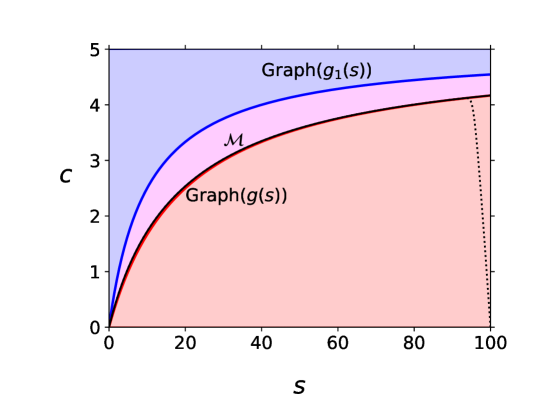
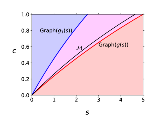
Figure 1: The $(s,c)$ phase plane geometry of the Michaelis–Menten reaction mechanism. The thick red curve, the graph of $g(s)$, is the QSS variety (i.e., the $c$-nullcline) and the thick blue curve, the graph of $g_{1}(s)$, is the $s$-nullcline. The thick black curve is the invariant slow manifold, $\mathcal{M}$. In the shaded violet region between the graphs is the slow invariant manifold, $\mathcal{M}$, that connects the stable equilibrium at the origin with a saddle equilibrium at infinity. The vector field in the red shaded region below Graph($g(s)$) satisfies $\dot{c}>0$ and $\dot{s}<0$. On Graph($g(s)$), $\dot{c}=0$ and $\dot{s}<0.$ In the magenta region that lies above Graph($g(s)$) and below Graph($g_{1}(s)$), $\dot{s}<0$ and $\dot{c}<0.$ On $g_{1}(s)$, $\dot{s}=0$ and $\dot{c}<0$. In the blue shaded region above Graph($g_{1}(s)$) and below $c=e_{0}$, $0<\dot{s}$ and $\dot{c}<0.$ The dotted black curve in the top panel is a single trajectory obtained via numerical integration of the mass action equations (1) with parameters (in arbitrary units): $s_{0}=100,e_{0}=5.0,k_{1}=1.0,k_{2}=k_{-1}=10.0$. The trajectory approaches and intercepts the graph of $g(s)$ at $t=t_{\rm cross}.$ For $t>t_{\rm cross}$, the trajectory lies above Graph($g(s))$, but below $\mathcal{M}$. Top: The trajectory enters the the magenta region and approaches $\mathcal{M}$ as time evolves forward. Bottom: Closeup of the top panel near the QSS variety. The trajectory still lies below $\mathcal{M}$, but becomes effectively indistinguishable from $\mathcal{M}$ as $t\to\infty$.

3 Critical estimates for the dynamics of the Michaelis–Menten reaction mechanism

One can rewrite system (1) as

$$\begin{array}[]{rcl}\dot{s}&=&-k_{1}e_{0}s+(k_{-1}+k_{1}s)c,\\ \dot{c}&=&-(k_{-1}+k_{2}+k_{1}s)(c-g(s)).\\ \end{array}$$ (13)

In the above system, $g(s)$ is given by (5). We are only interested in the solution with initial value $(s_{0},0)$, which starts below the graph of $g$. Since $\dot{c}\leq 0$ for $c\geq g(s)$, we have

$$c\leq\widetilde{c}:=\max_{0\leq s\leq s_{0}}g(s)=\dfrac{e_{0}s_{0}}{K_{M}+s_{0}}=\varepsilon_{SSl}\,s_{0}.$$ (14)

We will frequently use basic properties of differential inequalities (see, for instance, Walter [34, §9, Theorem 8]). For later use, we note two estimates for substrate concentration, $s$:

Lemma 3.

Let $s(t)$ be the first component of the solution of (13) with initial value $(s_{0},0)$. Then, for all $t\geq 0$ one has

$$s(t)\geq s_{0}\exp(-k_{1}e_{0}t),$$ (15)

and

$$s(t)\leq s_{0}\left(\cfrac{k_{-1}}{k_{-1}+k_{2}}+\cfrac{k_{2}}{k_{-1}+k_{2}}\exp\bigg{(}-\cfrac{k_{1}e_{0}K_{M}}{K_{M}+s_{0}}\cdot t\bigg{)}\right).$$ (16)

Proof.

The first estimate follows readily from $\dot{s}\geq-k_{1}e_{0}s$, $s(0)=s_{0}$. As for the second, from the first equation in (1), with (14), one finds

$$\dot{s}=-k_{1}(e_{0}-c)s+k_{-1}c\leq-k_{1}(e_{0}-\widetilde{c})s+k_{-1}\widetilde{c}.$$

Comparing $s$ with the solution of the linear differential equation

$$\dot{x}=k_{1}(e_{0}-\widetilde{c})x+k_{-1}\widetilde{c}=-\dfrac{k_{1}e_{0}K_{M}}{K_{M}+s_{0}}\,x+\dfrac{k_{-1}e_{0}s_{0}}{K_{M}+s_{0}},\quad x(0)=s_{0}$$

shows the assertion. ∎

Remark 2.

Note that the derivative of the right-hand side of (15) is equal to $-k_{1}e_{0}s_{0}$ at $t=0$, which agrees with $\dot{s}(0)$ in (1), while the right-hand side of (16) has derivative $-\dfrac{k_{2}}{k_{1}(K_{M}+s_{0})}\cdot k_{1}e_{0}s_{0}$, which is markedly different. From this perspective, the upper estimate is not optimal.

We will proceed in three steps. First, we estimate the distance of the solution to the slow manifold. In a second step, we obtain lower and upper approximations for $t_{\rm cross}$, and we compare exact and approximate solutions near the slow manifold in the third step. Throughout we will not impose any a priori assumptions concerning smallness of parameters — so most estimates are universally valid if not necessarily sharp — but indicate when such assumptions are made.

3.1 First Step: Approach to the slow manifold

We will employ two variants of a Lyapunov function approach. The first variant is based on established procedure [2, see, as an example, Section 2.1]. However, some adjustments are necessary, because system (1) with small parameter $e_{0}=\varepsilon e_{0}^{*}$ ($e_{0}^{*}$ some reference value) is not in Tikhonov standard form with separated slow and fast variables. We will restrict attention to the compact positively invariant rectangle defined by $0\leq s\leq s_{0}$ and $0\leq c\leq e_{0}^{*}$. By (14), we may further restrict attention to the rectangle defined by $0\leq s\leq s_{0}$ and $0\leq c\leq\widetilde{c}$. Consider

$$\cfrac{d}{dt}(c-g(s))^{2}=-2(k_{-1}+k_{2}+k_{1}s)(c-g(s))^{2}-2g^{\prime}(s)\dot{s}(c-g(s)).$$ (17)

Let $L:=c-g(s)$. By invoking $\dot{s}+\dot{c}=-k_{2}c$, we obtain with repeated use of (13):

$$\cfrac{d}{dt}L^{2} =-2(k_{-1}+k_{2}+k_{1}s))L^{2}-2g^{\prime}(s)\dot{s}\,L$$ (18a)

$$=-2(k_{-1}+k_{2}+k_{1}s)L^{2}+2g^{\prime}(s)\bigg{[}\dot{c}+k_{2}c\bigg{]}\,L$$ (18b)

$$=-2(k_{-1}+k_{2}+k_{1}s)L^{2}+2g^{\prime}(s)\bigg{[}-(k_{-1}+k_{2}+k_{1}s)\,L+k_{2}c\bigg{]}\,L$$ (18c)

$$=-2(k_{-1}+k_{2}+k_{1}s)L^{2}-2(k_{-1}+k_{2}+k_{1}s)g^{\prime}(s)L^{2}+2g^{\prime}(s)k_{2}c\,L$$ (18d)

$$\leq-2\bigg{[}\min_{s\in[0,s_{0}]}(k_{-1}+k_{2}+k_{1}s)(1+g^{\prime}(s))\bigg{]}L^{2}+2\max_{s\in[0,s_{0}]}|g^{\prime}(s)|\cdot k_{2}\widetilde{c}\cdot|L|.$$ (18e)

Now

$$g^{\prime}(s)=\cfrac{K_{M}e_{0}}{(K_{M}+s)^{2}}\geq 0;\quad\max_{s\in[0,s_{0}]}|g^{\prime}(s)|=\cfrac{e_{0}}{K_{M}},$$ (19)

therefore

$$\min_{s\in[0,s_{0}]}(k_{-1}+k_{2}+k_{1}s)(1+g^{\prime}(s))\geq\min_{s\in[0,s_{0}]}(k_{-1}+k_{2}+k_{1}s)=k_{-1}+k_{2}.$$

Altogether we obtain with (14)

$$\cfrac{d}{dt}L^{2}\leq-2(k_{-1}+k_{2})\cdot L^{2}+2\cfrac{e_{0}}{K_{M}}\cdot\dfrac{k_{2}e_{0}s_{0}}{K_{M}+s_{0}}\cdot|L|.$$ (20)

Next, we apply the Cauchy-Schwarz inequality

$$2\cfrac{e_{0}}{K_{M}}\cdot\dfrac{k_{2}e_{0}s_{0}}{K_{M}+s_{0}}\cdot|L|\leq\sigma L^{2}+\left(2\cfrac{e_{0}}{K_{M}}\cdot\dfrac{k_{2}e_{0}s_{0}}{K_{M}+s_{0}}\right)^{2}\cdot\dfrac{1}{2\sigma},$$

which holds for any $\sigma>0$. For $\sigma=k_{-1}+k_{2}$, this yields

$$\cfrac{d}{dt}L^{2}\leq-(k_{-1}+k_{2})\cdot L^{2}+\frac{1}{2}\cdot\ (k_{-1}+k_{2})\cdot\left(\varepsilon_{SSl}\cdot\varepsilon_{MM}\right)^{2}\cdot s_{0}^{2}.$$ (21)

Lemma 4.

Let $t_{0}\geq 0$ be given, with $L(t_{0})=L_{0}$. Then, for all $t\geq t_{0}$ one has

$$L^{2}\leq L_{0}^{2}\exp(-k_{1}K_{M}(t-t_{0}))+\frac{1}{2}\varepsilon_{SSl}^{2}\varepsilon_{MM}^{2}\left(1-\exp(-k_{1}K_{M}(t-t_{0}))\right).$$ (22)

In particular, with $t_{0}=0$ and $L(0)=e_{0}s_{0}/(s_{0}+K_{M})=s_{0}\varepsilon_{SSl}$ for the initial value $(s_{0},0)$,

$$\begin{array}[]{rcl}\dfrac{L^{2}}{s_{0}^{2}}&\leq&\varepsilon_{SSl}^{2}\left(\exp(-k_{1}K_{M}t)+\frac{1}{2}\varepsilon_{MM}^{2}(1-\exp(-k_{1}K_{M}t))\right)\\ &=&\varepsilon_{SSl}^{2}\left(\exp(-(k_{-1}+k_{2})t)+\frac{1}{2}\varepsilon_{MM}^{2}(1-\exp(-(k_{-1}+k_{2})t))\right).\end{array}$$ (23)

Proof.

Compare (21) with the differential equation

$$\cfrac{dV}{dt}=-(k_{-1}+k_{2})\cdot V+\frac{1}{2}(k_{-1}+k_{2})\varepsilon_{SSl}^{2}\varepsilon_{MM}^{2}\cdot s_{0}^{2}$$

for $V:=L^{2}$. The explicit solution of this linear equation for $V$ and a differential inequality argument (or Gronwall) yield the asserted estimates. ∎

Remark 3.

The first factor on the right hand side of (23) is the square of the Segel–Slemrod parameter $\varepsilon_{SSl}$, and the factor inside the second bracket is the square of the local timescale parameter $\varepsilon_{MM}$. Since $L/s_{0}$ is generally bounded by $\varepsilon_{SSl}$, the relevant parameter for the distance to the QSS manifold will be $\varepsilon_{MM}$. This and the above holds for any choice of parameters.

For a more detailed inspection, we assume $\varepsilon_{MM}<1$, so the right hand side of (23) decreases with $t$. Then, for all $t\geq\widehat{t}$,

$$\widehat{t}:=\dfrac{2}{k_{-1}+k_{2}}\cdot\log\left(\dfrac{(k_{-1}+k_{2})^{2}}{k_{1}k_{2}e_{0}}\right)=\dfrac{2}{k_{1}K_{M}}\log\dfrac{1}{\varepsilon_{MM}}$$ (24)

one obtains that

$$\dfrac{|c-g(s)|}{s_{0}}\leq\sqrt{\frac{3}{2}}\cdot\varepsilon_{SSl}\cdot\varepsilon_{MM}.$$ (25)

To verify the inequality, it suffices to do so for $t=\widehat{t}$, and this, in turn, follows from the fact that

$$\exp(-(k_{-1}+k_{2})t)={\varepsilon_{MM}}^{2}$$

is solved by $t=\widehat{t}$.

This provides a first estimate for the approach to the slow manifold.

Remark 4.

One may consider similar estimates for complex QSS, with no a priori reference to singular perturbations, in the system with substrate inflow:

$$\begin{array}[]{rclclcl}\dot{s}&=&k_{0}-k_{1}e_{0}s&+&(k_{-1}+k_{1}s)c\\ \dot{c}&=&k_{1}e_{0}s&-&(k_{-1}+k_{2}+k_{1}s)c.\\ \end{array}$$

Here, it is appropriate to choose initial values $s(0)=c(0)=0$. The chain of inequalities above works similarly, with the crucial difference that $\dot{s}=k_{0}-\dot{c}+k_{2}c$. So, the assumption $e_{0}=\varepsilon e_{0}^{*}$ will no longer result in an order $\varepsilon^{4}$ term in the analogue of(23) (unless $k_{0}$ is also of order $\varepsilon$); only order $\varepsilon^{2}$ can be salvaged. For more details, please see the discussion in Eilertsen et al. [9, Subsection 4.4].

For $t\leq t_{\rm cross}$ an alternative Lyapunov function approach is suggested by Lemma 1. We start with a variant of equation (17):

$$\cfrac{d}{dt}(c-g(s))=-(k_{-1}+k_{2}+k_{1}s)(c-g(s))-g^{\prime}(s)\dot{s}.$$ (26)

Again, let $L:=c-g(s)$. Similar to the derivation of Lemma 4, we find for $t\leq t_{\rm cross}$ (using $c-g(s)\leq 0$):

$$\cfrac{dL}{dt} =-(k_{-1}+k_{2}+k_{1}s))L-g^{\prime}(s)\dot{s}$$ (27a)

$$=-(k_{-1}+k_{2}+k_{1}s)L+g^{\prime}(s)\left(\dot{c}+k_{2}c\right)$$ (27b)

$$=-\left((1+g^{\prime}(s))(k_{-1}+k_{2}+k_{1}s)\right)L+k_{2}g^{\prime}(s)c$$ (27c)

$$=-\left((1+g^{\prime}(s))(k_{-1}+k_{2}+k_{1}s)\right)L+k_{2}g^{\prime}(s)(L+g(s)).$$ (27d)

So, we have

Lemma 5.

Consider the solution of (1) with initial value $(s_{0},0)$ at $t=0$. Then, for $0\leq t\leq t_{\rm cross}$,

$$\cfrac{dL}{dt}=-A\,L+B$$ (28)

with

$$\begin{array}[]{rcl}A:&=&k_{-1}+k_{2}+k_{1}s+g^{\prime}(s)(k_{-1}+k_{1}s),\\ B:&=&k_{2}g^{\prime}(s)g(s).\end{array}$$

Note that when $g(s)=c$ and $s>0$, then ${dL}/{dt}=k_{2}g^{\prime}(s)g(s)>0$.

3.2 Second Step: The crossing time

We will use Lemma 5 to compute upper and lower bounds, $t_{u}$ and $t_{\ell}$, such that $t_{\rm cross}\in[t_{\ell},t_{u}]$. The strategy will be to extract $t_{u}$ and $t_{\ell}$ from appropriate differential inequalities. We will express most of our estimates via the Segel–Slemrod parameter $\varepsilon_{SSl}$. Although — as mentioned in the Introduction — the parameters used by Briggs and Haldane, or by Reich and Selkov, would be equally applicable in any well-defined limit with $e_{0}\to 0$ (and all other parameters in a compact subset of the open positive orthant), the Segel–Slemrod parameter turns out to be the most convenient.

We first determine a lower bound $t_{\ell}$. By (5) and (19), we obtain

$$g(s)\leq\dfrac{e_{0}s_{0}}{K_{M}+s_{0}}\text{ and }g^{\prime}(s)\leq\dfrac{e_{0}}{K_{M}}\text{ for }0\leq s\leq s_{0}.$$

Now, with the notation of Lemma 5, we have

$$\begin{array}[]{rcl}A&=&k_{-1}+k_{2}+k_{1}s+\dfrac{e_{0}K_{M}}{(K_{M}+s)^{2}}(k_{-1}+k_{1}s)\\ &\leq&k_{1}(K_{M}+s)\left(1+\dfrac{e_{0}K_{M}}{(K_{M}+s)^{2}}\right)\\ &=&k_{1}(K_{M}+s)+k_{1}e_{0}\dfrac{K_{M}^{2}}{(K_{M}+s)^{2}}\\ &\leq&k_{1}(K_{M}+e_{0}+s_{0})=:A^{*},\end{array}$$

and furthermore

$$B\leq k_{2}\cdot\dfrac{e_{0}s_{0}}{K_{M}+s_{0}}\cdot\dfrac{e_{0}}{K_{M}}=:B^{*}.$$

Since for $t\leq t_{\rm cross}$ one has $L\leq 0$, the differential equation (28) implies the inequality

$$\dfrac{dL}{dt}\leq-A^{*}\,L+B^{*}.$$ (29)

Thus, defining $L^{*}$ by

$$\dfrac{dL^{*}}{dt}=-A^{*}L^{*}+B^{*},\quad L^{*}(0)=-g(s_{0}),$$

one obtains that $L(t)\leq L^{*}(t)$ for $0\leq t\leq t_{\rm cross}$. Explicitly,

$$\begin{array}[]{rcl}L^{*}&=&-\left(\dfrac{B^{*}}{A^{*}}+g(s_{0})\right)\exp(-A^{*}t)+\dfrac{B^{*}}{A^{*}}\\ \\ &=&s_{0}\varepsilon_{SSl}\left(-\left(1+\dfrac{k_{2}}{k_{1}K_{M}(1+\varepsilon_{SSl})}\varepsilon_{SSl}\right)\,\exp{(-(1+\varepsilon_{SSl})\lambda t)}+\dfrac{k_{2}}{k_{1}K_{M}(1+\varepsilon_{SSl})}\varepsilon_{SSl}\right),\end{array}$$ (30)

where $\lambda:=k_{1}(K_{M}+s_{0})$. Now define $t_{\ell}$ by $L^{*}(t_{\ell})=0$. A straightforward calculation shows

$$\begin{array}[]{rcl}t_{\ell}&=&\dfrac{1}{k_{1}(K_{M}+s_{0})(1+\varepsilon_{SSl})}\,\log\left(1+\dfrac{k_{-1}+k_{2}}{k_{2}}(1+\varepsilon_{SSl})\cdot\dfrac{1}{\varepsilon_{SSl}}\right)\\ &=&\dfrac{1}{(k_{1}s_{0}+k_{-1}+k_{2})(1+\varepsilon_{SSl})}\,\log\left(1+\dfrac{k_{-1}+k_{2}}{k_{2}}(1+\varepsilon_{SSl})\cdot\dfrac{1}{\varepsilon_{SSl}}\right)\end{array}$$ (31)

This provides a lower estimate:

Lemma 6.

For the solution of (1), with initial value $(s_{0},0)$, one has $t_{\rm cross}\geq t_{\ell}$.

Proof.

Assume that $t_{\rm cross}<t_{\ell}$, then $L(t_{\ell})>0$. This is a contradiction to $L(t_{\ell})\leq L^{*}(t_{\ell})=0$. ∎

Recall that Segel and Slemrod [29] introduced

$$t_{SSl}:=\dfrac{1}{k_{1}(K_{M}+s_{0})}=\dfrac{1}{k_{-1}+k_{2}+k_{1}s_{0}}$$ (32)

to estimate the duration of the fast transient. This defines the appropriate timescale at the very start, but as we show below, it cannot reflect the full transient phase.

There is a slightly simplified estimate for $t_{\ell}$:

$$\begin{array}[]{rcl}t_{\ell}&=&t_{SSl}\dfrac{1}{1+\varepsilon_{SSl}}\log\left(\dfrac{1}{\varepsilon_{SSl}}\bigg{[}\dfrac{k_{1}K_{M}}{k_{2}}+\varepsilon_{SSl}\left(\dfrac{k_{1}K_{M}}{k_{2}}+1\right)\bigg{]}\right)\\ &\geq&t_{SSl}\dfrac{1}{1+\varepsilon_{SSl}}\log\left(\dfrac{1}{\varepsilon_{SSl}}\dfrac{k_{1}K_{M}}{k_{2}}\right)\\ &=&t_{SSl}\dfrac{1}{1+\varepsilon_{SSl}}\log\left(\dfrac{1}{\varepsilon_{SSl}}\right)+\log\left(\dfrac{k_{1}K_{M}}{k_{2}}\right)\\ &\geq&t_{SSl}\left(1-\varepsilon_{SSl}\right)\left(\log\left(\dfrac{1}{\varepsilon_{SSl}}\right)+\log\left(\dfrac{k_{1}K_{M}}{k_{2}}\right)\right).\\ \end{array}$$

Therefore, we may define

$$t_{\ell}^{\dagger}:=t_{SSl}(1-\varepsilon_{SSl})\left(\log\left(\dfrac{1}{\varepsilon_{SSl}}\right)+\log\left(\dfrac{k_{-1}+k_{2}}{k_{2}}\right)\right)$$ (33)

as a lower estimate for the crossing time. In the limiting case $e_{0}\to 0$, an asymptotic expansion of the right-hand side yields

$$t_{\ell}^{\dagger}\sim t_{SSl}\left[\log\dfrac{1}{\varepsilon_{SSl}}+\log\dfrac{k_{-1}+k_{2}}{k_{2}}+o(1)\right]$$ (34)

For the slow timescale, chosen (in consistency with the choice of the small parameter) as $\tau=\varepsilon_{SSl}t$, the above observations yield a lower estimate with leading term of order $\varepsilon_{SSl}\cdot\log(1/\varepsilon_{SSl})$ in the asymptotic expansion.

Remark 5.

At this point, it seems appropriate to reconsider the notion “onset of slow dynamics” for the case of small $\varepsilon_{SSl}$. For system (1), we noted that the distinguished time $t_{\rm cross}$ (see, Lemma 1 and the following ones) is a natural choice from a biochemical perspective. But singular perturbation theory does not provide a precisely defined time for the onset of the slow phase. The following two observations are based on a fundamental criterion for slow dynamics, namely closeness of the solution to the QSS manifold:

• Equation (30) shows that $|L^{*}(t_{SSl})/s_{0}|\approx\varepsilon_{SSl}\exp(-1)$. But, since $|L/s_{0}|$ can always be estimated above by terms of order $\varepsilon_{SSl}$ [see, (23)], this inequality does not indicate closeness to the QSS manifold. Thus, the onset of slow dynamics cannot be assumed near $t_{SSl}$, and the Segel–Slemrod time $t_{SSl}$ seriously underestimates the duration of the transient phase.

• One may replace the condition $L^{*}(t)=0$ from (30) by an order $\varepsilon_{SSl}^{2}$ closeness condition, requiring $L^{*}(t)/s_{0}\geq-M\cdot\varepsilon_{SSl}^{2}$, with some positive constant $M$, as the defining characteristic of the slow phase. A provisional definition of $t_{ons}$ by $L^{*}(t_{ons})/s_{0}=-M\cdot\varepsilon_{SSl}^{2}$ yields $L^{*}(t)/s_{0}\geq-M\cdot\varepsilon_{SSl}^{2}$ for $t_{ons}\leq t\leq t_{\rm cross}$. Similar to the derivation of (31), one obtains an estimate

  $$t_{ons}=t_{SSl}\log(M^{*}/\varepsilon_{SSl})+\cdots$$ (35)

  with some constant $M^{*}$, and the dots representing higher order terms. Thus, we have the same lowest order asymptotic term $\log(1/\varepsilon_{SSl})$ as for $t_{\ell}^{\dagger}$.

We proceed to estimate initial substrate depletion:

Proposition 1.

One has the inequality

$$\dfrac{s(t_{\ell}^{\dagger})}{s_{0}}\leq\dfrac{k_{-1}}{k_{-1}+k_{2}}+\dfrac{k_{2}}{k_{-1}+k_{2}}\exp\left(-\dfrac{\varepsilon_{SSl}K_{M}}{(K_{M}+s_{0})}(1-\varepsilon_{SSl})\cdot\log\left(\dfrac{k_{1}K_{M}}{\varepsilon_{SSl}k_{2}}\right)\right).$$

Moreover, when

$$\varepsilon_{SSl}\cdot\log\left(\dfrac{k_{1}K_{M}}{k_{2}\varepsilon_{SSl}}\right)<1,$$ (36)

then

$$\dfrac{s_{0}-s_{\rm cross}}{s_{0}}\geq\dfrac{s_{0}-s(t_{\ell}^{\dagger})}{s_{0}}\geq\dfrac{k_{2}}{2k_{1}(K_{M}+s_{0})}\varepsilon_{SSl}(1-\varepsilon_{SSl})\log\left(\dfrac{k_{1}K_{M}}{\varepsilon_{SSl}k_{2}}\right).$$ (37)

Proof.

The estimate for $s(t_{\ell}^{\dagger})$ is obtained by substitution of $t_{\ell}^{\dagger}$ in (16). As for (37), the first inequality holds because $s$ is decreasing with $t$. Then one directly obtains

$$\dfrac{s_{0}-s(t_{\ell}^{\dagger})}{s_{0}}\geq\dfrac{k_{2}}{k_{-1}+k_{2}}\left(1-\exp(-\alpha)\right)$$

with

$$\alpha:=\dfrac{\varepsilon_{SSl}K_{M}}{K_{M}+s_{0}}(1-\varepsilon_{SSl})\cdot\log\left(\dfrac{k_{1}K_{M}}{\varepsilon_{SSl}k_{2}}\right)<\varepsilon_{SSl}\cdot\log\left(\dfrac{k_{1}K_{M}}{\varepsilon_{SSl}k_{2}}\right).$$

Condition (36) implies that $\alpha<1$, and the exponential series and the Leibniz criterion show that

$$\exp(-\alpha)\leq 1-\alpha+\alpha^{2}/2\leq 1-\alpha/2.$$

This estimate yields the second assertion. ∎

Remark 6.

The estimate in Proposition 1 can be improved, subject to more restrictive assumptions on $\varepsilon_{SSl}$. Replacing (36) by

$$\varepsilon_{SSl}\cdot\log\left(\dfrac{k_{1}K_{M}}{\varepsilon_{SSl}k_{2}}\right)<r$$ (38)

for some $r,\,0<r\leq 1$, it is straightforward to see that

$$\dfrac{s_{0}-s_{\rm cross}}{s_{0}}\geq(1-r/2)\,\dfrac{k_{2}}{k_{1}}\dfrac{\varepsilon_{SSl}}{K_{M}+s_{0}}(1-\varepsilon_{SSl})\log\left(\dfrac{k_{1}K_{M}}{\varepsilon_{SSl}k_{2}}\right)$$ (39)

in this case. This suggests a simplified asymptotic estimate for $s_{\rm cross}$ by setting, for instance, $r=\sqrt{\varepsilon_{SSl}}$ and keeping only lowest order terms,

$$\dfrac{s_{0}-s_{\rm cross}}{s_{0}}\geq\dfrac{k_{2}}{k_{1}(K_{M}+s_{0})}\varepsilon_{SSl}\left[\log\left(\dfrac{1}{\varepsilon_{SSl}}\right)+\log\left(\dfrac{k_{1}K_{M}}{k_{2}}\right)\right]+\cdots$$

In comparison, the asymptotic expansion of the right-hand side of (37) starts with

$$\dfrac{k_{2}}{2k_{1}(K_{M}+s_{0})}\varepsilon_{SSl}(1-\varepsilon_{SSl})\log\left(\dfrac{k_{1}K_{M}}{\varepsilon_{SSl}k_{2}}\right)\sim\dfrac{k_{2}}{2k_{1}(K_{M}+s_{0})}\varepsilon_{SSl}\left[\log\dfrac{1}{\varepsilon_{SSl}}+\log\dfrac{k_{1}K_{M}}{k_{2}}\right]+\cdots$$ (40)

It turns out below that the (removable) factor $\cfrac{1}{2}$ is less problematic for estimates than the factor $\cfrac{k_{2}}{k_{1}(K_{M}+s_{0})}$.

Remark 7.

Thus, in the case of small $\varepsilon_{SSl}$, for $(s_{0}-s_{\rm cross})/s_{0}$ one has a lower estimate by an expression asymptotic to $\varepsilon_{SSl}\log(1/\varepsilon_{SSl})$. Notably, this estimate indicates that the relative substrate depletion at crossing time is not of order $\varepsilon_{SSl}$. The widely held assumption in the literature (see, e.g. Segel & Slemrod [29]) about negligibility of the substrate depletion in the pre-QSS phase should be seen from this perspective.

Moreover, upon replacing $t_{\rm cross}$ by a differently chosen onset time $t_{ons}$ as in (35), the argument in the proof of the Proposition, with Lemma 3 shows that

$$\dfrac{s_{0}-s(t_{ons})}{s_{0}}\geq\dfrac{k_{2}}{2k_{1}(K_{M}+s_{0})}\varepsilon_{SSl}\log\left(\dfrac{M^{*}}{\varepsilon_{SSl}}\right)+\cdots$$ (41)

whenever $\varepsilon_{SSl}\log\left(\dfrac{M^{*}}{\varepsilon_{SSl}}\right)<1$. Thus, the lowest order of the asymptotic expansion remains unchanged.

We now turn to upper bounds for $t_{\rm cross}$. For technical reasons, since our argument requires a positive lower estimate for $g(s)$, we fix an auxiliary constant $0<q<1$ and consider the interval $[q\,s_{0},\,s_{0}]$. Then,

$$g(s)\geq\dfrac{qe_{0}s_{0}}{K_{M}+qs_{0}}\text{ and }g^{\prime}(s)\geq\dfrac{e_{0}K_{M}}{(K_{M}+s_{0})^{2}}\quad\text{for}\quad qs_{0}\leq s\leq s_{0}.$$

Therefore,

$$A\geq k_{1}(qs_{0}+K_{M})=:A_{*},$$

and

$$B\geq k_{2}\dfrac{qe_{0}s_{0}}{K_{M}+qs_{0}}\cdot\dfrac{e_{0}K_{M}}{(K_{M}+s_{0})^{2}}=:B_{*}$$

when $qs_{0}\leq s\leq s_{0}$.

Hence, for $0\leq t\leq t_{\rm cross}$ and $s(t)\geq qs_{0}$, one has

$$\dfrac{dL}{dt}\geq-A_{*}L+B_{*},$$ (42)

and defining $L_{*}$ by

$$\dfrac{dL_{*}}{dt}=-A_{*}L_{*}+B_{*},\quad L_{*}(0)=-g(s_{0}),$$

the usual differential inequality argument shows $L\geq L_{*}$. Explicitly,

$$L_{*}=-\left(\dfrac{B_{*}}{A_{*}}+g(s_{0})\right)\exp(-A_{*}t)+\dfrac{B_{*}}{A_{*}}.$$

Define $t_{u}=t_{u}(q)$ by $L_{*}(t_{u}(q))=0$, thus

$$t_{u}(q)=\dfrac{1}{k_{1}(K_{M}+qs_{0})}\,\log\left(1+C(q)\cdot\dfrac{1}{\varepsilon_{SSl}}\right),\quad\text{with}\quad C=C(q):=\dfrac{1}{q}\cdot\dfrac{(k_{-1}+k_{2}+qk_{1}s_{0})^{2}}{k_{2}(k_{-1}+k_{2})}.$$ (43)

With the inequality

$$\dfrac{1}{q}<C(q)<\dfrac{C^{*}}{q},\quad C^{*}:=C(1)=\dfrac{(k_{-1}+k_{2}+k_{1}s_{0})^{2}}{k_{2}(k_{-1}+k_{2})}=\dfrac{k_{1}(K_{M}+s_{0})^{2}}{k_{2}K_{M}},$$ (44)

we obtain a more convenient estimate for $t_{u}(q)$:

$$\begin{array}[]{rcl}t_{u}(q)&=&t_{SSl}\dfrac{K_{M}+s_{0}}{K_{M}+qs_{0}}\log\left(1+\dfrac{C(q)}{\varepsilon_{SSl}}\right)\\ &\leq&t_{SSl}\dfrac{1}{q}\,\log\left(1+\dfrac{1}{\varepsilon_{SSl}}\dfrac{C^{*}}{q}\right).\end{array}$$

This gives rise to the upper estimate

$$t_{u}^{\dagger}(q):=t_{SSl}\dfrac{1}{q}\,\log\left(1+\dfrac{1}{\varepsilon_{SSl}}\dfrac{C^{*}}{q}\right)\geq t_{u}(q).$$ (45)

For later use, we note

$$\log\left(1+\dfrac{1}{\varepsilon_{SSl}}\dfrac{C^{*}}{q}\right)=\dfrac{1}{q}\log\dfrac{1}{\varepsilon_{SSl}}+\log\dfrac{C^{*}}{q}+\log\left(1+\dfrac{q\varepsilon_{SSl}}{C^{*}}\right)$$

and obtain in the limit $\varepsilon_{SSl}\to 0$ the asymptotic expansion

$$t_{u}^{\dagger}(q)=t_{SSl}\dfrac{1}{q}\,\log\left(1+\dfrac{1}{\varepsilon_{SSl}}\dfrac{C^{*}}{q}\right)\sim\frac{1}{q}t_{SSl}\left[\log\dfrac{1}{\varepsilon_{SSl}}+\log\dfrac{C^{*}}{q}+o(1)\right].$$ (46)

Equation (43) provides an upper estimate for the crossing time, subject to an additional condition:

Lemma 7.

Given $0<q<1$, assume that the solution of (1), with initial value $(s_{0},0)$, satisfies $s(t_{u}(q))\geq qs_{0}$. Then, $t_{\rm cross}\leq t_{u}(q)\leq t_{u}^{\dagger}(q)$.

Proof.

Assume that $t_{\rm cross}>t_{u}(q)$, then $L_{*}(t_{\rm cross})>0$ and consequently $L(t_{\rm cross})>0$; a contradiction. ∎

As will be seen below, the condition imposed in Lemma 7 will imply restrictions on $\varepsilon_{SSl}$.

Modulo the hypothesis of Lemma 7, we get an upper estimate for $t_{\rm cross}$ which is asymptotic to $\log(1/\varepsilon_{SSl})$, and complements the lower estimate $t_{\ell}$ with the same asymptotics. This clarifies the asymptotic behavior of $t_{\rm cross}$ as $\varepsilon_{SSl}\to 0$.

Still, criteria are needed to satisfy the hypothesis of the Lemma. The first step to obtain such criteria is to apply Lemma 3 for $t=t_{u}^{\dagger}(q)$. By straightforward calculations, one finds the first estimate in the following proposition:

Proposition 2.

One has

$$\dfrac{s(t_{u}^{\dagger}(q))}{s_{0}}\geq\exp\left(-\dfrac{1}{q}\varepsilon_{SSl}\log\left(1+\dfrac{1}{\varepsilon_{SSl}}\cdot\dfrac{C^{*}}{q}\right)\right).$$ (47)

Moreover, when

$$\varepsilon_{SSl}\log\left(1+\dfrac{1}{\varepsilon_{SSl}}\cdot\dfrac{C^{*}}{q}\right)<q$$

then

$$\dfrac{s_{0}-s_{\rm cross}}{s_{0}}\leq\dfrac{s_{0}-s(t_{u}^{\dagger}(q))}{s_{0}}\leq\dfrac{1}{q}\varepsilon_{SSl}\log\left(1+\dfrac{C^{*}}{q}\cdot\dfrac{1}{\varepsilon_{SSl}}\right).$$ (48)

Proof.

There remains estimate (48). The first inequality follows from monotonicity of $t\mapsto s(t)$. When the stated condition holds then

$$\gamma:=\dfrac{1}{q}\varepsilon_{SSl}\log\left(1+\dfrac{1}{\varepsilon_{SSl}}\cdot\dfrac{C^{*}}{q}\right)<1,$$

and therefore $\exp(-\gamma)>1-\gamma$ by the exponential series and the Leibniz criterion. Substitution yields the assertion. ∎

Analogous to the derivation of expansion (46) in the limiting case $\varepsilon_{SSl}\to 0$ one obtains an expansion of the right-hand side of equation (48), up to terms of order $o(\varepsilon_{SSl})$:

$$\dfrac{1}{q}\varepsilon_{SSl}\log\left(1+\dfrac{1}{\varepsilon_{SSl}}\cdot\dfrac{C^{*}}{q}\right)\sim\dfrac{1}{q}\left[\varepsilon_{SSl}\log\dfrac{1}{\varepsilon_{SSl}}+\varepsilon_{SSl}\log\dfrac{C^{*}}{q}+\cdots\right].$$ (49)

Equation (47), in view of $\lim_{x\to 0+}x\log(1/x)=0$, shows that for any fixed $q$ the condition $s(t_{u}^{\dagger}(q))\geq qs_{0}$ holds for sufficiently small $\varepsilon_{SSl}$.

There remains to determine usable explicit bounds for $\varepsilon_{SSl}$ for given $q$. We aim here at providing simple workable, rather than optimal, conditions:

Proposition 3.

Let $q\geq\frac{1}{2}$, such that

$$4q\log(1/q)\cdot\log(4C^{*})<1.$$

Assume that

$$\varepsilon_{SSl}<\exp(-1)\quad{\rm and}\quad\varepsilon_{SSl}\leq\frac{9}{16}\left(q\log(1/q)\right)^{2}.$$

Then, $s(t_{u}^{\dagger}(q))\geq qs_{0}$ and consequently $t_{\rm cross}\leq t_{u}^{\dagger}(q)$.

Proof.

By Lemma 7, it is sufficient to prove the inequality $s(t_{u}^{\dagger}(q))\geq qs_{0}$. By (47), this holds whenever

$$\exp\left(-\dfrac{1}{q}\varepsilon_{SSl}\log\left(1+\dfrac{C^{*}}{q}\cdot\dfrac{1}{\varepsilon_{SSl}}\right)\right)\geq q.$$

Equivalently

$$\dfrac{1}{q}\varepsilon_{SSl}\log\left(1+\dfrac{C^{*}}{q}\cdot\dfrac{1}{\varepsilon_{SSl}}\right)\leq\log\dfrac{1}{q},$$

or

$$\varepsilon_{SSl}\log\left(1+\dfrac{C^{*}}{q}\cdot\dfrac{1}{\varepsilon_{SSl}}\right)\leq q\log\dfrac{1}{q}.$$ (50)

Rewrite the left hand side as

$$\begin{array}[]{rcl}\varepsilon_{SSl}\log\left(1+\dfrac{C^{*}}{q}\cdot\dfrac{1}{\varepsilon_{SSl}}\right)&=&\varepsilon_{SSl}\log\left(\dfrac{1}{\varepsilon_{SSl}}\left(\varepsilon_{SSl}+\dfrac{C^{*}}{q}\right)\right)\\ &=&\varepsilon_{SSl}\log\left(\dfrac{1}{\varepsilon_{SSl}}\right)+\varepsilon_{SSl}\log\left(\varepsilon_{SSl}+\dfrac{C^{*}}{q}\right)\\ &\leq&\varepsilon_{SSl}\log\left(\dfrac{1}{\varepsilon_{SSl}}\right)+\varepsilon_{SSl}\log\left(2\cdot\dfrac{C^{*}}{q}\right)\\ &\leq&\varepsilon_{SSl}\log\left(\dfrac{1}{\varepsilon_{SSl}}\right)+\varepsilon_{SSl}\log(4C^{*}),\\ \end{array}$$

where we used $C^{*}\geq 1>\varepsilon_{SSl}$ and $\frac{1}{2}\leq q<1$. In view of $\varepsilon_{SSl}\log(1/\varepsilon_{SSl})\leq\sqrt{\varepsilon_{SSl}}$, the inequality (50) holds whenever

$$\sqrt{\varepsilon_{SSl}}+\varepsilon_{SSl}\log(4C^{*})\leq q\log\dfrac{1}{q}.$$ (51)

For the remainder of this proof, we abbreviate $A:=\log(4C^{*})$ and $B:=q\log\dfrac{1}{q}$. Let $\theta$ be the positive number with $A\theta^{2}+\theta=B$. Then, for any $\varepsilon_{SSl}\leq\theta^{2}$, the inequality (51) holds. Now, the solution of the above quadratic equation with $AB<1/4$, Taylor expansion and the Leibniz criterion show

$$\theta=\frac{1}{2A}\left(-1+\sqrt{1+4AB}\right)\geq\frac{1}{2A}\left(-1+1+\frac{4AB}{2}-\frac{16A^{2}B^{2}}{8}\right),$$

hence

$$\delta\geq B(1-AB)\geq\frac{3}{4}B.$$

Thus, inequality (51) holds whenever $\varepsilon_{SSl}\leq(\frac{3}{4}B)^{2}$. ∎

The role of the constant $q$ is mostly auxiliary. It serves to ensure the applicability of Proposition 3, but actual estimates e.g. of $s(t_{u}^{\dagger}(q))$ will rely on Proposition 2.

Example 1.

We consider one particular setting for the purpose of illustration. Assume that

$$C^{*}=\dfrac{(k_{-1}+k_{2}+k_{1}s_{0})^{2}}{k_{2}(k_{-1}+k_{2})}\leq 250.$$

This condition covers a wide range of reaction parameters, for instance it is satisfied whenever $s_{0}\leq 5K_{M}$ and $k_{-1}\leq 5k_{2}$. Then, the requirement on $q$ in Proposition 3 is satisfied whenever $q\geq 0.97$. For $q=0.97$. one finds the condition $\varepsilon_{SSl}\leq 4.9\cdot 10^{-4}$.

Rather than $t_{u}^{\dagger}(q)$, one may consider a slightly weaker, but more convenient estimate. Fix $\varepsilon_{SSl}$ such that $s(t_{u}^{\dagger}(q))\geq qs_{0}$. We will prove that the relative error upon replacing $t_{u}^{\dagger}(q)$ by

$$t_{u}^{\dagger}(1)=\dfrac{1}{k_{1}(K_{M}+s_{0})}\log\left(1+\dfrac{k_{1}(K_{M}+s_{0})^{3}}{k_{2}K_{M}e_{0}}\right)=t_{SSl}\log\left(1+\dfrac{C^{*}}{\varepsilon_{SSl}}\right)$$ (52)

is approximately equal to $(1-q)$ when $q$ approaches $1$.

Lemma 8.

One has

$$0\leq\dfrac{t_{u}^{\dagger}(q)-t_{u}^{\dagger}(1)}{t_{u}^{\dagger}(q)}\leq\dfrac{1-q}{q}\cdot\dfrac{1+\log(1+C^{*}/(q\,\varepsilon_{SSl}))}{\log(1+C^{*}/(q\,\varepsilon_{SSl}))}.$$

Proof.

We abbreviate $A=C^{*}/\varepsilon_{SSl}$ and consider the function

$$q\mapsto f(q):=\frac{1}{q}\log(1+A/q),$$

noting $t_{u}^{\dagger}(q)=t_{SSl}f(q)$. The derivative

$$f^{\prime}(q)=-\frac{1}{q^{2}}\left(\log(1+A/q)+\dfrac{A}{A+q}\right)$$

is an increasing function of $q$. By the mean value theorem, one has $f(q)-f(1)=(q-1)f^{\prime}(q^{*})$ for some $q^{*}$ between $q$ and $1$. Hence, by monotonicity and with $A/(A+q)<1$,

$$f(q)-f(1)\leq(1-q)\left|f^{\prime}(q)\right|\leq\frac{1-q}{q^{2}}\left(\log(1+A/q)+1\right).$$

The assertion follows. ∎

We also note an asymptotic expansion as $\varepsilon_{SSl}\to 0$:

$$\begin{array}[]{rcl}t_{u}^{\dagger}(1)&\sim&t_{SSl}\left[\log\dfrac{1}{\varepsilon_{SSl}}+\log\left(\dfrac{k_{1}K_{M}}{k_{2}}\left(\dfrac{K_{M}+s_{0}}{K_{M}}\right)^{2}\right)+o(1)\right]\\ &\sim&t_{SSl}\left[\log\dfrac{1}{\varepsilon_{SSl}}+\log\left(\dfrac{k_{-1}+k_{2}}{k_{2}}\left(\dfrac{k_{-1}+k_{2}+k_{1}s_{0}}{k_{-1}+k_{2}}\right)^{2}\right)+o(1)\right].\end{array}$$ (53)

The numerical simulations underlying Figure 2 illustrate that $t_{u}^{\dagger}(1)$ is a quite good approximation of the crossing time.

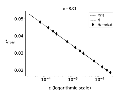
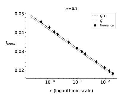
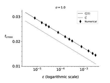
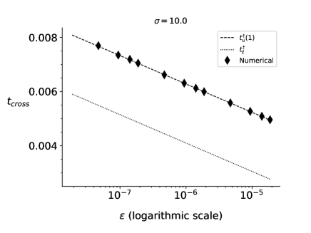
Figure 2: Numerical simulations indicate that $t_{u}^{\dagger}(1)$, defined in (52), is a reasonable estimation of $t_{\rm cross}$ when $e_{0}\ll K_{M}$. In all panels, $e_{0}\in[0.025,0.05,0.075,0.1,0.25,0.5,0.75,1.0,2.5,5.0,7.5,10]$, $k_{1}=1.0$, $k_{2}=k_{-1}=100$, thus $K_{M}=200$, and $\sigma=s_{0}/K_{M}$. The parameter $\varepsilon$ corresponds to the Reich-Selkov parameter $\varepsilon_{RS}=e_{0}/K_{M}$. The solid black diamonds are the numerically estimated crossing times. The densely dashed line is obtained from (52). The dotted line is obtained from (34). Top Left: $s_{0}=2$. Top Right: $s_{0}=20$. Bottom Left: $s_{0}=200$. Bottom Right: $s_{0}=2000$. Observe the noticeable difference between (53) and (34) when $s_{0}$ is much larger than $K_{M}$. This is due to the difference in the constant terms of the expansions. One also sees that the lower estimate $t_{\ell}^{\dagger}$ from (34) is worse than the upper estimate; compare Remark 2.

Remark 8.

Observe that $t_{u}^{\dagger}(1)$ corresponds to the estimate $T_{\rm in}$ from Noethen & Walcher [20, Lemma 4], but with an additional factor $(K_{M}+s_{0})/K_{M}$ nested inside the logarithm. The presence of this term is relevant: the solution slows down significantly – especially in the $c$-direction – near the $c$-nullcline in regions where $K_{M}\ll s$. In these regions, the solution will travel nearly horizontally and below the QSS manifold for an extended period of time before finally crossing. Moreover, the vanishing of $K_{M}$ gives rise to a line of equilibrium points at $c=e_{0}$. In this limiting case, the crossing time $t_{\rm cross}$ tends to infinity for any trajectory for which $c(0)\neq e_{0}$. This fact is reflected by the term $(K_{M}+s_{0})/K_{M}$ in the expression for $t_{u}^{\dagger}(1)$.

Finally, it may be appropriate to look at the substrate depletion during the transitory phase from a general perspective: As shown by equations (35) and (45) (setting $q=1$), the onset time for the slow dynamics will in any case be of the type

$$t^{*}_{ons}=t_{SSl}\log\dfrac{M}{\varepsilon_{SSl}}+\cdots$$ (54)

with some positive constant $M$. With slight modifications of Propositions 1 and 2 one arrives at

$$\widehat{M}_{1}\cdot\varepsilon_{SSl}\,\log\dfrac{1}{\varepsilon_{SSl}}+\cdots\leq\dfrac{s_{0}-s(t_{ons}^{*})}{s_{0}}\leq\widehat{M}_{2}\cdot\varepsilon_{SSl}\,\log\dfrac{1}{\varepsilon_{SSl}}+\cdots,$$ (55)

with suitable constants $\widehat{M}_{i}$. Thus, as $\varepsilon_{SSl}\to 0$ we have the asymptotic order $\varepsilon_{SSl}\,\log(1/\varepsilon_{SSl})$ for the relative initial substrate depletion.

3.3 Third Step: Error estimates for the approximation

We now turn toward global error estimates for the reduction. As in the previous subsection, we will express most estimates in terms of the Segel–Slemrod parameter $\varepsilon_{SSl}$.

For $t\geq t_{\rm cross}$, we consider the familiar Michaelis–Menten equation, augmented by an error term. We start from

$$\dot{s}=-k_{1}e_{0}s+(k_{-1}+k_{1}s)g(s)+(k_{-1}+k_{1}s)(c-g(s)).$$ (56)

Lemma 9.

For all $t\geq t_{\rm cross}$, the $s$ entry of the solution of (1) with initial value $(s_{0},0)$ satisfies

$$\begin{array}[]{rcccccl}\dot{s}&\geq&-\dfrac{k_{1}k_{2}e_{0}s}{k_{-1}+k_{2}+k_{1}s};&&&&\\ \dot{s}&\leq&-\dfrac{k_{1}k_{2}e_{0}s}{k_{-1}+k_{2}+k_{1}s}&+&\frac{1}{\sqrt{2}}k_{1}e_{0}s_{0}\cdot\bigg{(}\cfrac{k_{-1}+k_{1}s_{0}}{k_{-1}+k_{2}+k_{1}s_{0}}\bigg{)}\cdot\bigg{(}\cfrac{k_{1}k_{2}e_{0}}{(k_{-1}+k_{2})^{2}}\bigg{)}&=:&U(s).\\ \end{array}$$ (57)

Proof.

For the first inequality note that $c-g(s)\geq 0$ for $t\geq t_{\rm cross}$. For the second inequality, using (21) with $L(t_{\rm cross})=0$, one obtains

$$\dfrac{L^{2}}{s_{0}^{2}}\leq\frac{1}{2}\,\left(\varepsilon_{MM}\varepsilon_{SSl}\right)^{2}\cdot\left(1-\exp{[-(k_{-1}+k_{2})(t-t_{\rm cross})]}\right)\leq\frac{1}{2}\,\left(\varepsilon_{MM}\varepsilon_{SSl}\right)^{2}$$ (58)

for all $t\geq t_{\rm cross}$, thus one has $L/s_{0}\leq\frac{1}{\sqrt{2}}\varepsilon_{SSl}\varepsilon_{MM}$, with

$$\begin{array}[]{rcccccl}\dot{s}&=&-k_{1}e_{0}s+(k_{1}s+k_{-1})g(s)&+&(k_{-1}+k_{1}s)(c-g(s))&&\\ &\leq&-\dfrac{k_{1}k_{2}e_{0}s}{k_{-1}+k_{2}+k_{1}s}&+&\cfrac{1}{\sqrt{2}}\dfrac{k_{-1}+k_{1}s}{(k_{-1}+k_{1}s_{0})}\dfrac{k_{1}e_{0}s_{0}(k_{-1}+k_{1}s_{0})}{(k_{-1}+k_{2}+k_{1}s_{0})}\cdot\dfrac{k_{1}k_{2}e_{0}}{(k_{-1}+k_{2})^{2}}&&\\ &\leq&-\dfrac{k_{1}k_{2}e_{0}s}{k_{-1}+k_{2}+k_{1}s}&+&\cfrac{1}{\sqrt{2}}k_{1}e_{0}s_{0}\cdot\dfrac{k_{-1}+k_{1}s_{0}}{(k_{-1}+k_{2}+k_{1}s_{0})}\dfrac{k_{1}k_{2}e_{0}}{(k_{-1}+k_{2})^{2}}&=&U(s),\\ \end{array}$$ (59)

∎

Defining the equilibrium dissociation constant of enzyme-substrate complex as

$$K_{S}:=\dfrac{k_{-1}}{k_{1}},$$ (60)

one may rewrite

$$U(s)=-\dfrac{k_{2}e_{0}s}{K_{M}+s}+\frac{1}{\sqrt{2}}e_{0}s_{0}\left(\dfrac{K_{S}+s_{0}}{K_{M}+s_{0}}\right)\cdot\dfrac{k_{2}e_{0}}{K_{M}^{2}}.$$

Remark 9.

By the same token, one obtains an estimate for product formation:

$$\begin{array}[]{rcccccl}\dot{p}&=&k_{2}g(s)&+&k_{2}(c-g(s))&&\\ &\leq&\dfrac{k_{1}k_{2}e_{0}s}{k_{-1}+k_{2}+k_{1}s}&+&\cfrac{1}{\sqrt{2}}\dfrac{k_{1}k_{2}e_{0}s_{0}}{(k_{-1}+k_{2}+k_{1}s_{0})}\cdot\dfrac{k_{1}k_{2}e_{0}}{(k_{-1}+k_{2})^{2}}&&\\ &\leq&\dfrac{k_{1}k_{2}e_{0}s}{k_{-1}+k_{2}+k_{1}s}&+&\cfrac{1}{\sqrt{2}}k_{1}e_{0}s_{0}\cdot\dfrac{k_{-1}+k_{1}s_{0}}{(k_{-1}+k_{2}+k_{1}s_{0})}\cdot\dfrac{k_{1}k_{2}e_{0}}{(k_{-1}+k_{2})^{2}}&=&\widetilde{U}(s).\\ \end{array}$$ (61)

For the following fix $\widetilde{t}\geq t_{\rm cross}$. By differential inequality arguments, we will estimate the difference of the $s$ entry of the solution of (1) with initial values $(\widetilde{s},\widetilde{c})):=(s(\widetilde{t}),c(\widetilde{t}))$ – which is just a time shift of the solution of (1) with initial values $(s_{0},0)$ – and the Michaelis–Menten equation with initial value $\widetilde{s}$. We will base our estimates on the auxiliary result below.

Lemma 10.

Let $a$, $b$ and $c$ be positive real numbers, $x_{0},\,t_{0}\in\mathbb{R}$ and consider the initial value problems

$$\begin{array}[]{rclcl}\dot{x}&=&-\dfrac{cx}{x+a}+b&,&x(t_{0})=x_{0};\\ \dot{y}&=&-\dfrac{cy}{y+a}&,&y(t_{0})=x_{0};\\ \dot{z}&=&-\dfrac{cz}{z+a}&,&z(t_{0})=z_{0}>x_{0}.\end{array}$$

Then,

1. For all $t>t_{0}$, one has $x(t)-y(t)>0$.

2. Additionally, assume that $x_{0}>ab/(c-b)$. Then, $x(t)$ decreases for all $t>t_{0}$. We find that

   $$x(t)-y(t)\leq\dfrac{b\cdot(x_{0}+a)^{2}}{ac}\cdot\left(1-\exp\left[-\dfrac{ac}{(x_{0}+a)^{2}}\,(t-t_{0})\right]\right)\leq\dfrac{b\cdot(x_{0}+a)^{2}}{ac}$$

3. For all $t>t_{0}$, one has

   $$0<z(t)-y(t)\leq(z_{0}-x_{0})\cdot\exp\left[-\dfrac{ac}{(z_{0}+a)^{2}}\,(t-t_{0})\right]\leq z_{0}-x_{0}.$$

Proof.

Part (a), due to $x(0)=y(0)$, follows directly from a standard result on differential inequalities.

Turning to the proof of part (b), note that $x^{*}=ab/(c-b)$ is the only stationary point of the differential equation for $x$. So, the solution with initial value $x_{0}>x^{*}$ is strictly decreasing and converges to this point. Now, we have

$$\begin{array}[]{rcl}\cfrac{d}{dt}\left(x-y\right)&=&-c\left(\dfrac{x}{x+a}-\dfrac{y}{y+a}\right)+b\\ &=&-c\dfrac{a(x-y)}{(x+a)(y+a)}+b\\ &\leq&-\dfrac{ac}{(x_{0}+a)^{2}}\,(x-y)+b.\end{array}$$

Compare this with the solution of the initial value problem

$$\dot{v}=-\dfrac{ac}{(x_{0}+a)^{2}}v+b,\quad v(0)=0$$

to obtain the assertion. As for part (c), the first inequality is immediate, while the second is verified by a variant of the previous argument, with the inequality

$$\begin{array}[]{rcl}\cfrac{d}{dt}\left(z-y\right)&=&-c\left(\dfrac{z}{z+a}-\dfrac{y}{y+a}\right)\\ &\leq&-\dfrac{ac}{(z_{0}+a)^{2}}\,(z-y).\end{array}$$

∎

Evaluating the constant in part (b) of Lemma 10 with $a=K_{M}$, $b=\frac{1}{\sqrt{2}}e_{0}s_{0}\left(\cfrac{k_{2}e_{0}}{K_{M}^{2}}\right)\cfrac{K_{S}+s_{0}}{K_{M}+s_{0}}$, $c=k_{2}e_{0}$ and $x_{0}=\widetilde{s}$, we obtain

$$\frac{1}{\sqrt{2}}s_{0}\cdot\dfrac{e_{0}}{K_{M}}\cdot\dfrac{K_{S}+s_{0}}{K_{M}+s_{0}}\dfrac{K_{M}+\widetilde{s}}{K_{M}}\cdot\dfrac{K_{M}+\widetilde{s}}{K_{M}} \leq\frac{1}{\sqrt{2}}s_{0}\cdot\dfrac{e_{0}}{K_{M}}\cdot\dfrac{K_{S}+s_{0}}{K_{M}+s_{0}}\left(\dfrac{K_{M}+s_{0}}{K_{M}}\right)^{2}$$

$$=\frac{1}{\sqrt{2}}s_{0}\cdot\varepsilon_{RS}\cdot\dfrac{(K_{M}+s_{0})(K_{S}+s_{0})}{K_{M}^{2}}.$$

Choosing a natural scaling (and omitting the factor $\frac{1}{\sqrt{2}}$), the parameter

$$\varepsilon_{L}:=\varepsilon_{RS}\dfrac{(K_{M}+s_{0})(K_{S}+s_{0})}{K_{M}^{2}}=\dfrac{e_{0}}{K_{M}}\dfrac{(K_{M}+s_{0})(K_{S}+s_{0})}{K_{M}^{2}}=\dfrac{k_{1}e_{0}}{k_{-1}+k_{2}}\dfrac{(k_{-1}+k_{2}+k_{1}s_{0})(k_{-1}+k_{1}s_{0})}{(k_{-1}+k_{2})^{2}}$$ (63)

provides an upper estimate for the long-term accuracy of the reduction. Note that the index indicates that the parameter was obtained from a linear differential inequality.

3.3.1 Estimates for the slow dynamics: Special case

In the application of the QSSA, it is generally assumed that there is an initial transient during which the substrate concentration remains approximately constant or changes slowly while the complex concentration builds up. This assumption – that the substrate concentration does not change significantly during this initial transient – is known as the reactant stationary approximation [16, 23]. The general assumption is that $s\approx s_{0}$ from $t=0$ until $t_{\rm cross}$. However, this a qualitative estimate. A more careful analysis is required in order to formulate a quantitative assertion concerning the validity of the reactant stationary approximation.

We first determine estimates given the special assumption that the substrate concentration at the start of the slow phase is exactly known. In view of Lemma 9 and Lemma 10, we then obtain

Proposition 4.

Denote by $s(t)$ the first component of the solution of (1) with initial value $(s_{0},0)$ at $t=0$. Moreover, let $\widetilde{t}\geq t_{\rm cross}$, $\widetilde{s}:=s(\widetilde{t})$ and define $\underline{s}$, resp. $\overline{s}$ by

$$\begin{array}[]{rcccl}\dot{\underline{s}}&=&-\dfrac{k_{2}e_{0}\underline{s}}{K_{M}+\underline{s}}&,&\underline{s}(\widetilde{t})=\widetilde{s};\\ \dot{\overline{s}}&=&-\dfrac{k_{1}k_{2}e_{0}\overline{s}}{K_{M}+\overline{s}}+\sqrt{2}k_{1}e_{0}s_{0}\cdot\bigg{(}\cfrac{k_{-1}+k_{1}s_{0}}{k_{-1}+k_{2}+k_{1}s_{0}}\bigg{)}\cdot\bigg{(}\cfrac{k_{1}k_{2}e_{0}}{(k_{-1}+k_{2})^{2}}\bigg{)}&,&\overline{s}(\widetilde{t})=\widetilde{s}.\\ \end{array}$$ (64)

Then, for all $t\geq\widetilde{t}$, we have

$$\underline{s}(t)\leq s(t)\leq\overline{s}(t)$$ (65)

and

$$\overline{s}(t)-s(t)\leq s_{0}\cdot\varepsilon_{L};\quad s(t)-\underline{s}(t)\leq s_{0}\cdot\varepsilon_{L}.$$ (66)

Proof.

To prove (65), use Lemma 9. Moreover, parts (a) and (b) of Lemma 10 show that

$$\overline{s}(t)-\underline{s}(t)\leq\frac{1}{\sqrt{2}}s_{0}\varepsilon_{RS}\cdot\dfrac{K_{S}+s_{0}}{K_{M}+s_{0}}\cdot\left(\dfrac{K_{M}+\widetilde{s}}{K_{M}}\right)^{2}\leq\frac{1}{\sqrt{2}}s_{0}\varepsilon_{RS}\cdot\dfrac{(K_{M}+s_{0})(K_{S}+s_{0})}{K_{M}^{2}}<s_{0}\,\varepsilon_{L},$$

which in combination with (65) proves (66). ∎

There is a different approach to upper and lower estimates for $s$ in the slow regime, based on Lemma 2, with the parameter $\delta^{*}$ defined in (11). We also utilize the explicit solution of the Michaelis–Menten equation via the Lambert W function, as obtained in Schnell & Mendoza [26].

Proposition 5.

Denote by $s(t)$ the first component of the solution of (1) with initial value $(s_{0},0)$ at $t=0$. Moreover let $\widetilde{t}\geq t_{\rm cross}$, $\widetilde{s}:=s(\widetilde{t})$, and $1>\delta\geq\delta^{*}$.

1. Define $\underline{s}$, resp. $\overline{s}$ by

   $$\begin{array}[]{rcccl}\dot{\underline{s}}&=&-\dfrac{k_{2}e_{0}\underline{s}}{K_{M}+\underline{s}}&,&\underline{s}(\widetilde{t})=\widetilde{s};\\ \dot{\overline{s}}&=&-(1-\delta)\dfrac{k_{1}k_{2}e_{0}\overline{s}}{K_{M}+\overline{s}}&,&\overline{s}(\widetilde{t})=\widetilde{s}.\\ \end{array}$$ (67)

   Then, for all $t\geq\widetilde{t}$, we have

   $$\underline{s}(t)\leq s(t)\leq\overline{s}(t).$$ (68)

2. Explicitly, setting

   $$A:=\dfrac{\widetilde{s}}{K_{M}}\exp\dfrac{\widetilde{s}}{K_{M}},\quad T:=\dfrac{k_{2}e_{0}(t-\widetilde{t})}{K_{M}}$$

   we obtain

   $$\begin{array}[]{rcl}\underline{s}(t)&=&K_{M}\,W(A\exp(-T))\\ \overline{s}(t)&=&K_{M}\,W(A\exp(-T)\exp(\delta T))\\ \end{array}$$ (69)

We turn to estimating $\overline{s}-\underline{s}$, using basic properties of the Lambert $W$ function that can for instance be found in Mező [18, Section 1].

Lemma 11.

With the notation introduced in Lemma 5, one has

$$\begin{array}[]{rclcl}\overline{s}-\underline{s}&\leq&K_{M}\log\left(1+W(Ae^{-T})(e^{\delta T}-1)\right)&\leq&K_{M}W(Ae^{-T})(e^{\delta T}-1)\\ \overline{s}-\underline{s}&\leq&K_{M}\log\left(1+Ae^{-T}(e^{\delta T}-1)\right)&\leq&K_{M}Ae^{-T}(e^{\delta T}-1)\\ \end{array}$$ (70)

for all $t\geq\widetilde{t}$.

Proof.

Let us abbreviate $\alpha:=Ae^{-T}$ and $\beta:=\alpha e^{\delta T}$. Then, with a known identity for $W^{\prime}$ and monotonicity of $W$, one sees

$$\begin{array}[]{rcl}K_{M}^{-1}\left(\overline{s}-\underline{s}\right)&=&\displaystyle\int_{\alpha}^{\beta}W^{\prime}(x)\,{\rm d}x=\int_{\alpha}^{\beta}\dfrac{{\rm d}x}{x+\exp(W(x))}\\ &\leq&\displaystyle\int_{\alpha}^{\beta}\dfrac{{\rm d}x}{x+\exp(W(\alpha))}=\log(x+\exp(W(\alpha))|_{\alpha}^{\beta}\\ &=&\log\left(\dfrac{1+\beta e^{-W(\alpha)}}{1+\alpha e^{-W(\alpha)}}\right)=\log\left(1+\dfrac{\alpha e^{-W(\alpha)}(e^{\delta T}-1)}{1+\alpha e^{-W(\alpha)}}\right)\\ &\leq&\log\left(1+\alpha e^{-W(\alpha)}(e^{\delta T}-1)\right)\\ &=&\log\left(1+W(\alpha)(e^{\delta T}-1)\right),\\ \end{array}$$

where we have used the defining identity for $W$ in the last step. This shows the first inequality, and the remaining ones follow from $0\leq W(x)\leq x$ and $\log(1+x)\leq x$ when $x\geq 0$. ∎

Presently, we will use only the last inequality from (70) to obtain a global error estimate.

Proposition 6.

With the assumptions and notation from Proposition 5, for all $t\geq\widetilde{t}$ the following inequalities hold:

$$0\leq s-\underline{s}\leq\overline{s}-\underline{s}\leq s_{0}\,\exp\left(\dfrac{s_{0}}{K_{M}}-1\right)\cdot\dfrac{\delta}{1-\delta}\leq s_{0}\,\exp\left(\dfrac{s_{0}}{K_{M}}-1\right)\cdot\dfrac{\delta^{*}}{1-\delta^{*}}=:s_{0}\cdot\varepsilon_{W}.$$ (71)

Proof.

By elementary arguments, the function $T\mapsto e^{-T}(e^{\delta T}-1)$, with derivative $T\mapsto e^{-T}\left(1-(1-\delta)e^{\delta T}\right)$ attains its maximum at $T^{*}=-\log(1-\delta)/\delta\geq 1$, with value

$$\widetilde{s}\exp(\widetilde{s}/K_{M})\exp(-T^{*})\cdot\dfrac{\delta}{1-\delta}\leq s_{0}\exp(s_{0}/K_{M})\exp(-1)\cdot\dfrac{\delta}{1-\delta}.$$

The assertion follows. ∎

Remark 10.

The index in $\varepsilon_{W}$ should remind of its derivation via the Lambert $W$ function. This may not be a particularly user-friendly parameter, but one can replace it by more convenient estimates. For instance, in case $\varepsilon_{RS}\leq 0.1$, by (12) one may choose $\delta\leq\frac{10}{9}\varepsilon_{RS}$, and proceed to obtain the estimate

$$\varepsilon_{LW}\leq\frac{5}{4}\exp\left(\dfrac{s_{0}}{K_{M}}-1\right)\cdot\varepsilon_{RS}.$$

Remark 11.

For all $t\geq\widetilde{t}$, we thus obtained the estimates $|s-\underline{s}|\leq s_{0}\varepsilon_{W}$, and $|s-\underline{s}|\leq s_{0}\varepsilon_{L}$. Either of these may be better, given the circumstances. Both estimates are rigorous, and moreover $\widetilde{t}\geq t_{\rm cross}$, for which rigorous lower estimates are available. However, we have to note that their derivation involves some simplified estimates, so they may not be optimal. Indeed, extensive numerical experiments point to an upper estimate

$$\varepsilon_{opt}:=\dfrac{K_{S}+s_{0}}{K_{M}+s_{0}}\varepsilon_{SSl}\leq\varepsilon_{SSl},$$ (72)

but with our toolbox a rigorous proof for this conjecture does not seem possible (see, Figure 3 and also Figure 7 below).

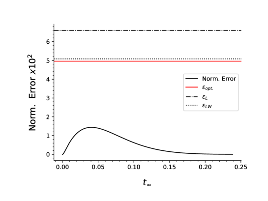
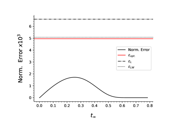
Figure 3: Numerical simulations suggest that (72) provides an upper bound on the normalized error between the $s$-component of the mass action equations and the sQSSA for the complete time course when initial conditions lie on the QSS variety, $c=g(s)$. In both panels, the black curve is the numerically-estimated normalized absolute error, $|\xi-s|/s_{0}$. The dash-dotted and dotted lines correspond to $\varepsilon_{L}$ and $\varepsilon_{LW}$, respectively, and the red line is $\varepsilon_{\rm opt.}$ On the $x$-axis, $t$ has been mapped to $t_{\infty}=1-1/\log(t+e)$, and initial conditions for the mass action equations and the sQSSA satisfy $(s,c)(0)=(s,c)(t_{\rm cross})$ and $\xi(0)=s(t_{\rm cross})$, respectively ($t_{\rm cross}$ is estimated numerically). Top: The parameters used in the simulation are (in arbitrary units): $s_{0}=10.0$, $e_{0}=10.0$, $k_{1}=2.0$, $k_{2}=100.0$ and $k_{-1}=100.0$. Bottom: The parameters used in the simulation are (in arbitrary units): $s_{0}=$$10.0$, $e_{0}=1.0$, $k_{1}=2.0$, $k_{2}=100.0$ and $k_{-1}=100.0$. The estimate $\varepsilon_{\rm opt}$ is not a sharp error estimate due to the choice of initial conditions.

3.3.2 Estimates for the slow dynamics: General case

Under the hypothesis that $\widetilde{t}$ and $\widetilde{s}=s(\widetilde{t})$ are known exactly, we obtained upper estimates for the approximation error. However, this idealizing assumption does not reflect the real-life setting of parameter identification for the reactant stationary approximation. Due to lack of complete information, experimental scientists effectively apply the Michaelis–Menten equation with some estimate $s^{*}$ for $s(\widetilde{t})$ valid under the reactant stationary approximation conditions [16]. This discrepancy must be accounted for by an additional term in the error estimate. Define $\xi$ by

$$\dot{\xi}=-\dfrac{k_{1}k_{2}e_{0}\xi}{k_{-1}+k_{2}+k_{1}\xi}=-\dfrac{k_{2}e_{0}\xi}{K_{M}+\xi},\quad\xi(\widetilde{t})=s^{*}\in(0,\,s_{0}].$$ (73)

Proposition 7.

Denote by $s(t)$ the first component of the solution of (1) with initial value $(s_{0},0)$ at $t=0$. Moreover, let $\widetilde{t}\geq t_{\rm cross}$, $\widetilde{s}:=s(\widetilde{t})$. Then, with $\underline{s}$ from (64) [or from (67)], for all $t\geq\widetilde{t}$, we have

$$|\xi-\underline{s}|\leq|s^{*}-\widetilde{s}|$$ (74)

and

$$|\xi-s|\leq|s^{*}-\widetilde{s}|+s_{0}\cdot\varepsilon_{L},$$ (75)

as well as

$$|\xi-s|\leq|s^{*}-\widetilde{s}|+s_{0}\cdot\varepsilon_{W}.$$ (76)

Proof.

For the first inequality use Lemma 10(c). For the second, note that

$$|\xi-s|\leq|\xi-\underline{s}|+|\underline{s}-s|\leq|s^{*}-\widetilde{s}|+|\underline{s}-s|$$

and use Propositions 4 and 6, respectively. ∎

Remark 12.

We should make the following observations for the above proposition:

1. Lemma 10 includes an exponentially decaying factor for the first term in the estimate. For practical experimental applications, this might be of little relevance for some enzyme catalyzed reactions, since in the scenario under consideration here this exponential decay will be slow and the initial transient will be fast.

2. The special case of (73) with $s^{*}=s_{0}$ seems to reflect the implicit assumption underlying many experiments, i.e., that there is no discernible loss in the transitory phase before the starting time $\widetilde{t}$ for measurements.

With the obvious (and to some extent controllable) choice $\widetilde{t}=t_{u}^{\dagger}(q)$, we obtain with Proposition 2:

Corollary 1.

Let $0<q<1$ and let $\varepsilon_{SSl}$ satisfy the hypotheses of Proposition 3. Then, for all $t\geq t_{u}^{\dagger}(q)$, one has

$$\begin{array}[]{rcl}\dfrac{|\xi-s|}{s_{0}}&\leq&\varepsilon_{SSl}\cdot\dfrac{1}{q}\log\left(1+\cfrac{1}{q}\dfrac{k_{1}(K_{M}+s_{0})^{2}}{k_{2}K_{M}}\dfrac{1}{\varepsilon_{SSl}}\right)+\varepsilon_{L};\\ \dfrac{|\xi-s|}{s_{0}}&\leq&\varepsilon_{SSl}\cdot\dfrac{1}{q}\log\left(1+\cfrac{1}{q}\dfrac{k_{1}(K_{M}+s_{0})^{2}}{k_{2}K_{M}}\dfrac{1}{\varepsilon_{SSl}}\right)+\varepsilon_{W}.\\ \end{array}$$ (77)

3.3.3 Assuming the standard quasi-steady-state approximation starts at $t=0$

In experiments, it is generally assumed that the substrate concentration does not change during the initial fast transient. Here we consider a different scenario. We assume that sQSSA is applicable from $t=0$. This reflects a widely used scenario in the literature, where one considers the reduced Michaelis–Menten equation with initial value $s_{0}$ at $t=0$ (see, the usual choice of initial value for (2) in the literature), and compares its solution to the true solution. This choice is compatible with the perspective of singular perturbation theory, because the relevant solution of (1) starts on the critical manifold with $c=0$. Experimentally it is not an unreasonable approximation, particularly for fast-acting enzymes, like carbonic anhydrase.

We will show for this scenario the approximation error is bounded by a term of order $\varepsilon_{SSl}$. More precisely:

Proposition 8.

Let $z(t)$ satisfy

$$\dot{z}=-\cfrac{k_{2}e_{0}z}{K_{M}+z},\quad z(0)=s_{0},$$

and denote by $s(t)$ the first component of the solution of (1) with initial value $(s_{0},0)$ at $t=0$.

1. Then, for all $t$ with $0\leq t\leq t_{\rm cross}$, one has $z(t)\geq s(t)$ and

   $$\cfrac{z-s}{s_{0}}\leq\varepsilon_{SSl}\cdot\bigg{(}\cfrac{s_{0}+K_{S}}{s_{\rm cross}+K_{M}}\bigg{)}\exp\left(k_{1}s_{0}\varepsilon_{SSl}t_{\rm cross}\right).$$ (78)

2. Let $0<q<1$ and $\varepsilon_{SSl}$ satisfy the hypotheses of Proposition 3. Then, for all $t$ with $0\leq t\leq t_{\rm cross}$, one has

   $$\cfrac{z-s}{s_{0}}\leq\varepsilon_{SSl}\cdot\cfrac{1}{q}\bigg{(}\cfrac{s_{0}+K_{S}}{s_{0}+K_{M}}\bigg{)}\exp\left(\frac{1}{q}k_{1}s_{0}t_{SSl}\cdot\varepsilon_{SSl}\log\left(1+\dfrac{1}{\varepsilon_{SSl}}\dfrac{C^{*}}{q}\right)\right),$$ (79)

   with $C^{*}$ from equation (44).

Proof.

Let

$$f(s,c)=:-k_{1}(e_{0}-c)s+k_{-1}c,$$

and recall that

$$f(s,\,g(s))=-\dfrac{k_{2}e_{0}s}{K_{M}+s},$$

with $g(s)=e_{0}s/(K_{M}+s)$ defined in (5). As in the proof of Lemma 10, one finds

$$g(z)-g(s) =e_{0}\bigg{(}\cfrac{z}{K_{M}+s}-\cfrac{s}{K_{M}+z}\bigg{)}$$

$$=e_{0}K_{M}\cdot\cfrac{z-s}{(K_{M}+s)(K_{M}+z)}.$$

Now, limit the temporal domain to $t\in[0,t_{\rm cross}]$, which implies $L:=c-g(s)\leq 0$ by Lemma 1, and furthermore

$$\dot{s}=f(s,c) =-k_{1}e_{0}s+(k_{-1}+k_{1}s)c,$$

$$\leq-k_{1}e_{0}s+(k_{-1}+k_{1}s)g(s),$$

$$=-\cfrac{k_{2}e_{0}s}{K_{M}+s}.$$

Therefore, $z\geq s$ for $t\leq t_{\rm cross}$ by the usual differential inequality argument.

With $c=g(s)+L$ one now has

$$\cfrac{d}{dt}(z-s) =f(z,g(z))-f(s,g(s)+L)$$

$$=f(z,g(z))-f(s,g(z))+f(s,g(z))-f(s,g(s)+L)$$

$$=-k_{1}(e_{0}-c)(z-s)+k_{1}(K_{S}+s)(g(z)-g(s)-L)$$

$$\leq-k_{1}(e_{0}-c)(z-s)+k_{1}(K_{S}+z)(g(z)-g(s)-L)$$

$$=-k_{1}(e_{0}-c)(z-s)-k_{1}(K_{S}+z)L+k_{1}(K_{S}+z)\cdot\cfrac{e_{0}K_{M}\cdot(z-s)}{(K_{M}+s)(K_{M}+z)}$$

$$\leq-k_{1}(e_{0}-c)(z-s)-k_{1}(K_{S}+z)L+k_{1}e_{0}(z-s),$$

which leaves us with:

$$\cfrac{d}{dt}(z-s)\leq k_{1}c(z-s)-k_{1}(K_{S}+s_{0})L,\quad\text{for all }t\leq t_{\rm cross}.$$ (83)

Since $c\leq s_{0}\varepsilon_{SSl}$ by (14), this ultimately implies

$$\cfrac{d}{dt}(z-s)\leq\varepsilon_{SSl}k_{1}s_{0}(z-s)-k_{1}(K_{S}+s_{0})L,\quad\text{for all }t\leq t_{\rm cross}.$$ (84)

Now, for $t\leq t_{\rm cross}$, one has with $f(s,c)\leq 0$ and $g^{\prime}(s)\geq 0$ and (13):

$$\begin{array}[]{rcl}\dfrac{dL}{dt}&=&k_{1}(K_{M}+s)L-g^{\prime}(s)\cdot f(s,c)\\ &\geq&k_{1}(K_{M}+s)L\geq k_{1}(K_{M}+s_{\rm cross})L,\end{array}$$

and therefore

$$L\geq-\dfrac{e_{0}s_{0}}{K_{M}+s_{0}}\,\exp\left(k_{1}(K_{M}+s_{\rm cross})t\right).$$

Consequently, we obtain:

$$\cfrac{d}{dt}(z-s)\leq\varepsilon_{SSl}k_{1}s_{0}\bigg{[}(z-s)+(K_{S}+s_{0})\exp(-k_{1}(K_{M}+s_{\rm cross})t)\bigg{]},\quad\text{for all }t\leq t_{\rm cross}.$$ (85)

Solving the corresponding linear differential equation yields for all $t\leq t_{\rm cross}$:

$$\begin{array}[]{rcl}\cfrac{z-s}{s_{0}}&\leq&\varepsilon_{SSl}\cdot\bigg{(}\cfrac{K_{S}+s_{0}}{K_{M}+s_{\rm cross}+\varepsilon_{SSl}s_{0}}\bigg{)}\bigg{(}\exp(k_{1}\varepsilon_{SSl}s_{0}t)-\exp(-k_{1}(K_{M}+s_{\rm cross})t)\bigg{)}\\ &\leq&\varepsilon_{SSl}\cdot\cfrac{K_{S}+s_{0}}{K_{M}+s_{\rm cross}}\exp(k_{1}\varepsilon_{SSl}s_{0}t)\\ &\leq&\varepsilon_{SSl}\cdot\cfrac{K_{S}+s_{0}}{K_{M}+s_{\rm cross}}\exp(k_{1}\varepsilon_{SSl}s_{0}t_{\rm cross}),\end{array}$$ (86)

which finishes the proof of part (a).

For part (b), we use $t_{\rm cross}\leq t_{u}^{\dagger}(q)$ [see, (45)], as well as $s_{\rm cross}\geq qs_{0}$ due to Lemma 7. ∎

Numerical results confirm that (86) yields a rather sharp bound on the normalized error accumulated as the phase-plane trajectory approaches the QSS manifold (see, Figure 4).

Remark 13.

The following observations should be made about our results:

1. Keeping only the lowest order term in (79), one has for $0\leq t\leq t_{\rm cross}$ that

   $$\cfrac{z-s}{s_{0}}\sim\varepsilon_{SSl}\cdot\frac{1}{q}\bigg{(}\cfrac{K_{S}+s_{0}}{K_{M}+s_{0}}\bigg{)}+o(\varepsilon_{SSl})=:\frac{1}{q}\varepsilon_{opt}+o(\varepsilon_{SSl})$$ (87)

   with $\varepsilon_{opt}$ defined in (72).

2. Numerical simulations confirm that (87) is a reliable estimation of the normalized error between $z$ and $s$ when $t\leq t_{\rm cross}$ (see, Figure 5).

3. With Propositions 5, 6 and 7 one sees that $|z-s|/s_{0}$ is of order $\varepsilon_{SSl}$ over the whole time range. Numerical simulations suggest that $\varepsilon_{opt}$ is a global upper bound (see, Figures 5 and 7).

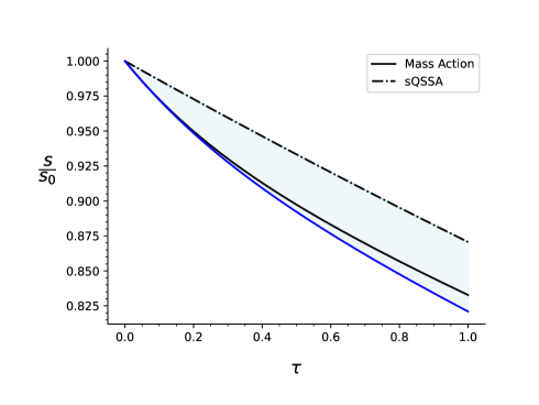
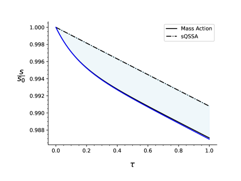
Figure 4: Numerical simulations confirm that (86) provides a sharp bound on the normalized error between the $s$-component of the mass action equations and the sQSSA. In both panels, the black curve is the numerical solution the mass action equations. The dashed/dotted curve is the numerical solution to the sQSSA. The admissible region given by the error bound (86) is shaded in blue. The blue line is the (normalized) numerical solution to the right-hand side of (86) with numerically-estimated (a priori) $q$ that corresponds to the upper boundary of (86). Time has been rescaled by $\tau=t/t_{\rm cross}$, where $t_{\rm cross}$ has been numerically-estimated. Top: The parameters used in the simulation are (in arbitrary units): $s_{0}=10.0$, $e_{0}=10.0$, $k_{1}=2.0$, $k_{2}=100.0$ and $k_{-1}=100.0$. Bottom: The parameters used in the simulation are (in arbitrary units): $s_{0}=100.0$, $e_{0}=1.0$, $k_{1}=2.0$, $k_{2}=100.0$ and $k_{-1}=100.0$.

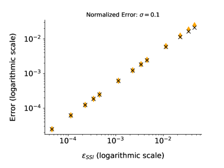
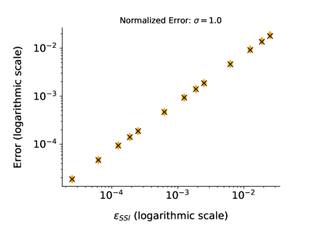
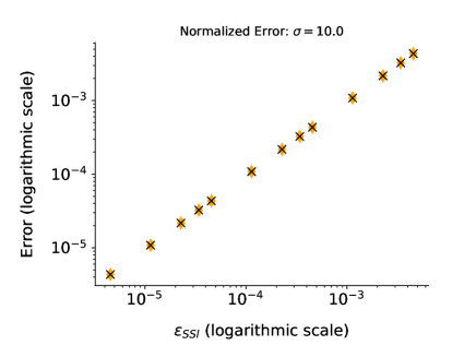
Figure 5: Numerical simulations confirm that (72) is a reasonable estimation of the normalized error when $t=t_{\rm cross}$ for small $\varepsilon_{SSl}$. In all panels, $e_{0}\in[0.025,0.05,0.075,0.1,0.25,0.5,0.75,1.0,2.5,5.0,7.5,10]$, $k_{1}=1.0,$ $k_{2}=k_{-1}=100.0$, thus $K_{M}=200$, and $\sigma=s_{0}/K_{M}$. The solid black crosses are the numerically–computed normalized error $|z-s|/s_{0}$ at $t=t_{\rm cross}$. The orange diamonds correspond to $\varepsilon_{opt}$. Top Left: $s_{0}=2.0$. Top Right: $s_{0}=20.0$. Bottom Left: $s_{0}=200.0$. Bottom Right: $s_{0}=2000.0$.

Remark 14.

The distinguishing difference between $\varepsilon_{SSl}$ and (87) is the appearance of the dimensionless factor

$$\eta=:\bigg{(}\cfrac{K_{S}+s_{0}}{K_{M}+s_{0}}\bigg{)}.$$

Recall that the specificity constant [14], $\Theta$, is defined as

$$\Theta=:\cfrac{k_{2}}{K_{M}}\leq k_{1}.$$ (88)

From (88) we can define the normalized specificity constant, $\bar{\Theta}=:\Theta/k_{1}$. Expressing $\eta$ in terms of $\bar{\Theta}$ and setting $\sigma:=s_{0}/K_{M}$ yields

$$\eta=\cfrac{1+\sigma-\bar{\Theta}}{1+\sigma},$$ (89)

and we conclude that (87) will be much smaller than $\varepsilon_{SSl}$ whenever $\bar{\Theta}\approx 1+\sigma$, which implies that $\sigma\ll 1$ and $\bar{\Theta}$ is close to $1$. This scenario can be useful in the study of functional effects of enzyme mutations [15]. Numerical simulations confirm that the normalized error may be far less than $\varepsilon_{SSl}$ when $\eta\ll 1$ (see, Figure 6).

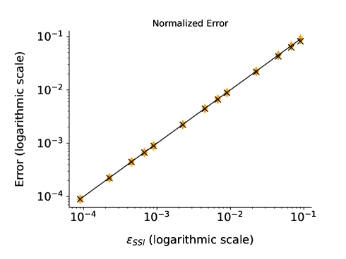
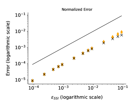
Figure 6: Numerical simulations confirm that (72) provides a sharp bound on the normalized error at $t=t_{\rm cross}$ between the $s$-component of the mass action equations and the sQSSA. In both panels the black line corresponds to $\log$(Error) $=\log(\varepsilon_{SSl})$ and $e_{0}\in[0.025,0.05,0.075,0.1,0.25,0.5,0.75,1.0,2.5,5.0,7.5,10]$. The orange diamonds correspond to (87) and the black crosses are the numerically-estimated normalized error between $s$ and $z$ at the numerically-estimated crossing time. Top: The parameters used in the simulation are (in arbitrary units): $s_{0}=10.0$, $e_{0}=1.0$, $k_{1}=2.0$, $k_{2}=1.0$ and $k_{-1}=100.0$. Bottom: The parameters used in the simulation are (in arbitrary units): $s_{0}=10.0$, $e_{0}=1.0$, $k_{1}=2.0$, $k_{2}=100.0$, and $k_{-1}=1.0$. Note that $\sigma\approx 0.1$ in both simulations. In the top panel, $\eta\approx 0.99$ and therefore the normalized error is approximately $\varepsilon_{SSl}$. On the other hand, $\eta\approx 0.1$ in the bottom panel, and therefore the normalized error at the crossing time is roughly one order of magnitude less than $\varepsilon_{SSl}.$

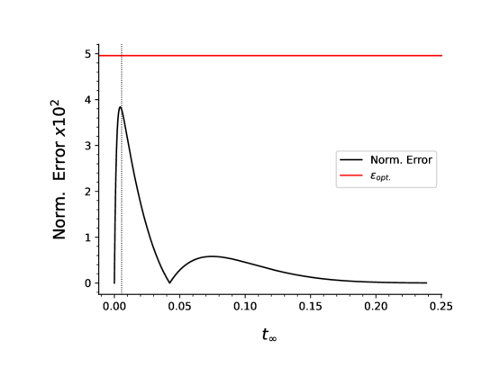
Figure 7: Assuming reactant stationary approximation from $t=0$: Numerical simulations suggest that (72) provides a sharp bound on the normalized error between the $s$-component of the mass action equations and the sQSSA for the complete time course. In both panels, the black curve is the normalized absolute error $|s-z|/s_{0}$. The red line is $\varepsilon_{\rm opt.}$ The initial conditions are $(s,c)(0)=(s_{0},0)$ and $z(0)=s_{0}$ and thus correspond to the assumption that the reactant stationary approximation is valid at the start of the reaction outlined in Section 3.3.3. The dotted vertical line demarcates the numerically–computed $t_{\rm cross}$. Note that $t$ has been mapped to $t_{\infty}=1-1/\log(t+e)$. Top: The parameters used in the simulation are (in arbitrary units): $s_{0}=10.0$, $e_{0}=10.0$, $k_{1}=2.0$, $k_{2}=100.0$ and $k_{-1}=100.0$. Bottom: The parameters used in the simulation are (in arbitrary units): $s_{0}=100.0$, $e_{0}=1.0$, $k_{1}=2.0$, $k_{2}=100.0$ and $k_{-1}=100.0$.

3.4 About the long-time quality of the approximation

The goal of the present work was to obtain workable upper estimates for the relative approximation error, $|(*-s)/s_{0}|$, where $*$ symbolizes the solution of some reduced equation, that are valid over the whole range of the slow dynamics. In their derivation, we deliberately chose simplified estimates which do not reflect that substrate concentration approaches $0$ as $t\to\infty$. Notably, in Lemma 10 and Lemma 11, we eventually disregarded slowly decaying terms which would imply convergence to zero for the approximations. So in these estimates the dynamics is not reflected well for very long times. (We recall that the parameters $\varepsilon_{MM}$ and $\varepsilon_{RS}$ govern the accuracy of the approximation for very long times; see Eilertsen et al. [10].) Our simplifications are justified since for the intended application – parameter identification – the time range directly after the onset of the slow dynamics is relevant, while the behavior as $t\to\infty$ is of less interest in the experimental setting.

4 Discussion: A view toward applications

Experimental enzymologists, and biochemists and analytical chemists may be less interested in mathematical technicalities and wish to focus on the essential results. Therefore, we will here summarize some essential application-relevant consequences from our theoretical considerations. These takeaways will remain technical for experimental scientists, but they are accessible to mathematical biologists and chemists, who work in close collaboration with experimental scientists. We provide quantitative error estimates, which may be relevant for a detailed study in application scenarios. In order to present the results without recourse to the technical sections, we will accept some redundancy. A quick-reference for the parameters defined in this paper can be found in the Appendix.

Thus, we consider the Michaelis-Menten system (1) for low initial enzyme concentration, so that the quasi-steady state approximation (2) holds with good accuracy. As a distinguished perturbation parameter we choose

$$\varepsilon_{SSl}=\dfrac{e_{0}}{K_{M}+s_{0}},$$

as proposed by Segel and Slemrod [29], and discuss the limiting case $\varepsilon_{SSl}\to 0$ (in detail, $e_{0}\to 0$ with the other parameters bounded above and below by positive constants).

Since $e_{0}$ and $s_{0}$ are controllable in a laboratory setting, the standard parameter estimation will provide approximate values for $K_{M}$ and $k_{2}$. In turn, this enables an educated guess for $\varepsilon_{SSl}$.

Our results provide error estimates for the approximation by the Michaelis-Menten equation (2). This may be taken as a vantage point toward error estimates for $k_{2}$ and $K_{M}$, and thus for consistency checks. Going beyond this, we obtain rigorous estimates for the onset time of the QSS regime, and for the substrate depletion during the initial transitory phase. This opens an approach to the identification of critical parameters required for the effective design of steady-state experiments.

We will only exhibit the two lowest-order terms in the asymptotic expansions with respect to $\varepsilon_{SSl}$, since these are dominant for sufficiently small initial enzyme concentration, and then further simplify these terms. The accuracy of approximation can — in any case — be gauged by a fuller analysis of the results in Section 3.

4.1 Onset of the slow dynamics

Generally, via singular perturbation theory one cannot define a fixed time for the end of the transitory phase. There always remains some freedom of choice when implementing a scale. As a definitive (biochemically relevant) time for the onset of the slow dynamics of the Michaelis–Menten reaction mechanism, following precedent, we chose the crossing time $t_{\rm cross}$, at which complex concentration is maximal. As noted in Remark 7, the familiar time

$$t_{SSl}=\dfrac{1}{k_{1}(s_{0}+K_{M})}$$

which seems to be suggested by Segel and Slemrod [29, equation (12)c], for the duration of the transient phase, leads to an underestimate for the asymptotics.

In this paper, we found:

• According to (33) and (34), an asymptotic lower estimate for the crossing time is given by

  $$t_{\ell}^{*}=t_{SSl}\,\left[\log\left(\dfrac{1}{\varepsilon_{SSl}}\right)+\log\dfrac{k_{-1}+k_{2}}{k_{2}}+\cdots\right]$$

• According to (45) and (46), an asymptotic upper estimate for the crossing time is given by

  $$t_{u}^{*}(q)=\frac{1}{q}t_{SSl}\left[\log\dfrac{1}{\varepsilon_{SSl}}+\log\dfrac{k_{1}(s_{0}+K_{M})^{2}}{qk_{2}K_{M}}+\cdots\right],$$

  where $q<1$ is fixed but may be taken arbitrarily close to $1$. To simplify this, we may approximate the upper estimate by

  $$t_{u}^{*}(1)=t_{SSl}\left[\log\dfrac{1}{\varepsilon_{SSl}}+\log\dfrac{k_{1}(s_{0}+K_{M})^{2}}{k_{2}K_{M}}+\cdots\right],$$

  since by Lemma 8, we may control the relative error by $1-q$ times a factor close to 1.

These considerations show that a lowest order approximation of the crossing time, hence of the onset time of slow dynamics, is given by

$$t_{\rm cross}\approx t^{\ast}:=t_{SSl}\,\log\left(\dfrac{1}{\varepsilon_{SSl}}\right).$$ (90)

4.2 Substrate depletion in the transient phase

Now, we estimate the relative substrate loss at $t_{\rm cross}$, thus $\Delta:=\dfrac{s_{0}-s_{\rm cross}}{s_{0}}$ to estimate the validity of the reactant stationary approximation. In Section 3, we found:

• From (37) and (40), one gets an asymptotic lower estimate

  $$\Delta\geq\dfrac{K}{2(s_{0}+K_{M})}\varepsilon_{SSl}\left[\log\dfrac{1}{\varepsilon_{SSl}}+\log\dfrac{k_{1}K_{M}}{k_{2}}+\cdots\right],$$

  noting (with Remark 6) that the factor $\frac{1}{2}$ could be discarded under slightly stricter hypotheses. The factor $K/(s_{0}+K_{M})$ stems from the estimate (16) in Lemma 3. As noted in Remark 2, the latter is not optimal.

• From (48) and (49), one gets an asymptotic upper estimate

  $$\Delta\leq\dfrac{1}{q}\varepsilon_{SSl}\left[\log\dfrac{1}{\varepsilon_{SSl}}+\log\dfrac{k_{1}(s_{0}+K_{M})^{2}}{qk_{2}K_{M}}+\cdots\right],$$

  with $q<1$ but arbitrarily close to $1$.

With similar arguments as those in Lemma 8, one sees that replacing $\Delta$ by

$$\dfrac{s_{0}-s_{\rm cross}}{s_{0}}\approx\Delta^{*}:=\varepsilon_{SSl}\left[\log\dfrac{1}{\varepsilon_{SSl}}+\log\dfrac{k_{1}(s_{0}+K_{M})^{2}}{k_{2}K_{M}}+\cdots\right]$$ (91)

involves a relative error equal to $1-q$ times a factor close to $1$. From the derivations via differential inequalities, there remains a gap between $\Delta^{*}$ and the lower estimate $K/(s_{0}+K_{M})\Delta^{*}$. Here, we resort to a heuristic argument. Given the accuracy of lower and upper estimates in Lemma 3 [note Remark 2], it seems preferable to choose $\Delta^{*}$ as the appropriate approximation. (This choice is also supported by extensive numerical simulations.) Keeping only the lowest order term, we note the approximation

$$\dfrac{s_{0}-s_{\rm cross}}{s_{0}}\approx\Delta^{**}:=\varepsilon_{SSl}\log\dfrac{1}{\varepsilon_{SSl}}$$ (92)

which depends only on the Segel–Slemrod parameter.

An educated guess for $s_{\rm cross}$ can be obtained based on $\varepsilon_{SSl}$. If progress curves are carried out in the laboratory, this opens a way to determine an approximation to the crossing time $t_{\rm cross}$, and further on $t_{SSl}$ and the reaction parameter $k_{1}$ as well as $k_{-1}$.

4.3 The approximation error assuming no transient substrate loss

The approximation of the $s$ component of the solution of (1) by the solution of (2) (after the transient phase) is correct only up to some error, and we determined rigorous bounds for this error. In turn, this information may be used toward estimating the errors in the determination of $K_{M}$ and $v_{\infty}$ from experimental data. First, we consider the scenario assuming no loss of substrate in the transient phase: $s(0\leq t\leq t_{\rm cross})=s_{0}$. This is considered the standard reactant stationary approximation scenario in enzyme kinetics. Allowing for somewhat weaker estimates by taking the limiting case with $q=1$ and discarding higher order terms as $e_{0}\to 0$, we arrive at “ultimate small parameters” for estimating the approximation error. The first step yields, depending on Proposition 4 or Proposition 6, respectively:

$$\varepsilon^{\dagger}_{L} :=\varepsilon_{SSl}\left(\log\left(\dfrac{k_{1}(K_{M}+s_{0})^{2}}{k_{2}K_{M}}\dfrac{1}{\varepsilon_{SSl}}\right)+\dfrac{(K_{M}+s_{0})^{2}(K_{S}+s_{0})}{K_{M}^{3}}\right),$$ (93)

$${\rm or}$$

$$\varepsilon^{\dagger}_{M} :=\varepsilon_{SSl}\left(\log\left(\dfrac{k_{1}(K_{M}+s_{0})^{2}}{k_{2}K_{M}}\dfrac{1}{\varepsilon_{SSl}}\right)+\exp\left(\frac{s_{0}}{K_{M}}-1\right)\dfrac{(K_{M}+s_{0})}{K_{M}}\right).$$ (94)

In a second step, we keep only lowest order terms in the asymptotics of $\varepsilon^{\dagger}$. With

$$\log\left(\dfrac{k_{1}(K_{M}+s_{0})^{2}}{k_{2}K_{M}}\dfrac{1}{\varepsilon_{SSl}}\right)=\log\left(\dfrac{k_{1}(K_{M}+s_{0})^{2}}{k_{2}K_{M}}\right)+\log\left(\dfrac{1}{\varepsilon_{SSl}}\right)$$

we ultimately obtain

$$\varepsilon^{\ddagger}=\varepsilon_{SSl}\log\left(\dfrac{1}{\varepsilon_{SSl}}\right).$$ (95)

Remarkably, in the asymptotic limit the error due to substrate depletion in the transitory phase (which is responsible for the logarithmic term) is dominant.

4.4 The approximation error assuming standard quasi-steady-state approximation starts at $t=0$

In Proposition 8, from this assumption we obtained an asymptotic error estimate (87) that is of order $\varepsilon_{SSl}$. Combining this with Proposition 4, resp. Proposition 6, and keeping only lowest order terms, we obtain

$$\varepsilon^{\S}_{L} :=\varepsilon_{SSl}\left(\dfrac{K_{S}+s_{0}}{K_{M}+s_{0}}+\dfrac{(K_{M}+s_{0})^{2}(K_{S}+s_{0})}{K_{M}^{3}}\right),$$ (96)

$${\rm or}$$

$$\varepsilon^{\S}_{M} :=\varepsilon_{SSl}\left(\dfrac{K_{S}+s_{0}}{K_{M}+s_{0}}+\exp\left(\frac{s_{0}}{K_{M}}-1\right)\dfrac{(K_{M}+s_{0})}{K_{M}}\right)$$ (97)

with $K_{S}=k_{-1}/k_{1}$. Beyond these rigorously proven asymptotic estimates, numerical simulations suggest a sharper bound

$$\varepsilon_{\rm opt}=\varepsilon_{SSl}\dfrac{K_{S}+s_{0}}{K_{M}+s_{0}}<\varepsilon_{SSl}.$$

Thus, while there may be problems with obtaining $K_{S}$ from experimental data, one may use $\dfrac{K_{S}+s_{0}}{K_{M}+s_{0}}<1$ and thus get error estimates involving only quantities that are controllable, or obtainable from fitting progress curves or initial rate experiments. In particular, this provides a mathematical foundation to the relevance of the Segel-Slemrod parameter $\varepsilon_{SSl}$.

4.5 Open challenges within the laboratory setting

The Michaelis–Menten equation,

$$\dot{s}=-\dot{p}=-\dfrac{k_{2}e_{0}s}{K_{M}+s},$$

involves two parameters, the Michaelis constant ($K_{M}$) and catalytic constant $(k_{2})$ when the initial enzyme concentration ($e_{0}$) and initial substrate concentration ($s_{0}$) are known and can be controlled.

In principle, experimental scientists can estimate $k_{2}$ and $K_{M}$ via steady-state initial rate experiments with the Michaelis–Menten equation, or steady-state progress curve experiments with the Schnell–Mendoza equation [26]. However, there is a fundamental problem with those parameter estimations. It requires to have prior knowledge of the duration of transient $t_{\rm cross}$ and substrate depletion in the transient phase $s(t=t_{\rm cross})$, assuming sufficiently small $\varepsilon_{SSl}$. The fundamental goal of the present paper is to provide rigorous estimates for $t_{\rm cross}$, $s(t=t_{\rm cross})$ as well as $\varepsilon_{SSl}$ from a mathematical perspective.

Generally, the role of our theoretical results is to provide consistency checks for experimental conclusions. Our estimates for the crossing times involve only parameters that are controllable or amenable to determination by experiments, though challenges remains in the unique estimation of $k_{1}$. In this respect, our mathematical results remain to be explored in the experimental laboratory setting. By assuming sufficiently small $\varepsilon_{SSl}$, our theoretical results might make possible to obtain an educated guess for $s_{\rm cross}$ by (92) in enzyme assays. By identifying the time when the guess for $s_{\rm cross}$ is attained, we could obtain an estimate for $t_{\rm cross}$, which in turn, with known $s_{0}$ and $K_{M}$, and equation (90), could provide an estimate for $k_{1}$. Our results could also be used to check the consistency of experimental results by measuring the end of the transition time, or the substrate depletion during the transient phase in steady-state experiments.

Interestingly, the same problem already was present with the Segel–Slemrod timescale $(k_{1}(s_{0}+K_{M}))^{-1}$, and it is actually an inherent feature of any parameter estimation that is solely based on the Michaelis–Menten equation (2). The essential new aspect of our work is that we obtained rigorous asymptotic expressions for the substrate loss in the transient phase, as well as for the approximation error, that only involve $\varepsilon_{SSl}=e_{0}/(K_{M}+s_{0})$. But rigorous experimental protocols require further quantitative information — e.g. about the onset of the slow time regime — that is not readily available. This remains an open problem for exploration in future work.

5 Appendix

5.1 A quick-reference guide

Tables 1 to 3 provide essential constants and critical parameters for the Michaelis–Menten reaction mechanism. These are pivotal for designing accurate laboratory measurements, such as initial rates and progress curves, for reliable parameter estimation.

Table 1 defines crucial steady-state constants of the Michaelis-Menten reaction. These are the constants generally estimated in the laboratory.

Table 2 introduces the foundational small parameter and fast timescale defined by Segel & Slemrod. These concepts are instrumental in estimating the key parameters discussed in this paper.

Table 3 serves as a quick reference for all critical parameters defined in this paper. Reliability indicators ($+$ for rigorous asymptotics, $++$ for asymptotics with rigorous upper and lower bounds) highlight the robustness of each estimate (details in Section 3). The Michaelis–Menten approximation error bound, $\varepsilon_{SSl}$, is weaker than the previous one, $\varepsilon_{opt}$, but does not involve $K_{S}$, which may be unavailable. The accuracy of these estimates improves with smaller $\varepsilon_{SSl}$, a parameter initially unknown.

In steady-state experiments, assuming a sufficiently small Segel-Slemrod parameter initially allows for estimating $K_{M}$ and $v_{\infty}$ using the Michaelis–Menten equation (2). If initial concentrations are known, this allows to calculate an estimate for $\varepsilon_{SSl}$ and performing a consistency check.

5.2 The Michaelis–Menten reaction mechanism with a low enzyme and substrate binding rate constant ($k_{1}\to 0$)

The case of low enzyme concentration in the Michaelis–Menten reaction mechanism is not the only one which leads to a singular perturbation reduction via Tikhonov and Fenichel. We can also obtain reductions in the limit $k_{2}\to 0$ (which will be discussed in future work) and in the limit $k_{1}\to 0$.

The case of low enzyme and substrate binding $k_{1}\to 0$ is of some interest since it represents the commonly expressed setting “$s_{0}\ll K_{M}$” in terms of singular perturbations (while letting $s_{0}\to 0$ does not). The arguments so far were motivated by the scenario with $e_{0}\to 0$, but all the estimates obtained in Sections 2 and 3 do hold, possibly upon rewriting some expressions involving $K_{M}$, without any restriction on the reaction rates and concentrations involved.

So here, we briefly summarize the pertinent results when $k_{1}\to 0$, while $e_{0}$ is bounded below. Thus, $k_{1}=\varepsilon k_{1}^{*}$ with $\varepsilon\to 0$. The “crossing Lemma”, Lemma 1 holds for all Michaelis–Menten type reaction mechanisms, so one may still employ the sQSS manifold given by $c=g(s)$ in (5) for the analysis of the system. Note that the first order approximation of the slow manifold is given by

$$c=\widehat{g}(s):=\dfrac{k_{1}e_{0}s}{k_{-1}+k_{2}},$$

but the discrepancy between $g$ and $\widehat{g}$ is of order $\varepsilon^{2}$, and the distinguished role of the sQSS manifold [defined by (5)] for the time course of complex concentration remains convenient in the analysis. One may also keep the Michaelis–Menten equation, in the version

$$\dot{s}=-\dfrac{k_{1}k_{2}e_{0}s}{k_{-1}+k_{2}+k_{1}s},$$

noting that the standard reduction procedure yields the right-hand side

$$-\dfrac{k_{1}k_{2}e_{0}s}{k_{-1}+k_{2}}=-\dfrac{k_{1}k_{2}e_{0}s}{k_{-1}+k_{2}+k_{1}s}+o(\varepsilon),$$

and for Tikhonov’s theorem higher-order terms on the right-hand side are irrelevant.

It seems appropriate to take $\varepsilon_{RS}=\dfrac{k_{1}e_{0}}{k_{-1}+k_{2}}$ as a benchmark here. As noted, the relevant expressions obtained in Section 3 remain unchanged, but we record some asymptotics with the dots denoting higher order terms with respect to $\varepsilon_{RS}$:

$$\begin{array}[]{rcl}\varepsilon_{SSl}&=&\varepsilon_{RS}+\cdots\\ t_{SSl}&=&\dfrac{1}{k_{-1}+k_{2}}+\cdots\\ t_{\ell}^{\dagger}&=&\dfrac{1}{k_{-1}+k_{2}}\left(\log\dfrac{1}{\varepsilon_{RS}}+\log\dfrac{k_{-1}+k_{2}}{k_{2}}+\cdots\right)\\ C^{*}&=&\dfrac{k_{-1}+k_{2}}{k_{2}}+\cdots\\ t_{u}^{\dagger}(1)&=&\dfrac{1}{k_{-1}+k_{2}}\left(\log\dfrac{1}{\varepsilon_{RS}}+\log\dfrac{k_{-1}+k_{2}}{k_{2}}+\cdots\right)\\ \varepsilon_{\infty}&=&\varepsilon_{RS}\cdot\dfrac{k_{-1}}{k_{-1}+k_{2}}+\cdots\\ \end{array}$$

For the substrate depletion during the transient phase, one gets from Proposition 2 and Lemma 8:

$$\dfrac{s_{0}-s_{\rm cross}}{s_{0}}\lesssim\varepsilon_{RS}\left(\log\dfrac{1}{\varepsilon_{RS}}+\log\dfrac{k_{-1}+k_{2}}{k_{2}}\right)+\cdots$$

We may summarize this by stating that in lowest order the dynamics is unaffected by initial substrate, in marked contrast to the low enzyme case.

References

- [1] V.I. Arnold: Ordinary Differential Equations. Springer–Verlag, Berlin (1992).
- [2] N. Berglund, B. Gentz: Noise-induced phenomena in slow-fast dynamical systems. A sample-paths approach. Springer, London (2006).
- [3] J.A Borghans, R.J de Boer, L.A. Segel: Extending the quasi-steady state approximation by changing variables. Bull. Math. Biol. 58, 43-–63 (1996)
- [4] G. E. Briggs, J. B. S. Haldane: A note on the kinetics of enzyme action. Biochem. J., 19, 338–339 (1925).
- [5] M.S. Calder, D. Siegel: Properties of the Michaelis-Menten mechanism in phase space. J. Math. Anal. Appl. 339, 1044–-1064 (2008).
- [6] H. Cartan: Elementary theory of analytic functions of one or several complex variables. Addison–Wesley, Reading, Mass. (1963).
- [7] C. Chicone: Ordinary differential equations with applications. edition. Springer–Verlag, New York (2006).
- [8] A. Cornish-Bowden: Fundamentals of Enzyme Kinetics, edition. Wiley–VCH, Weinheim, Germany (2012).
- [9] J. Eilertsen, M.R. Roussel, S. Schnell, S. Walcher: On the quasi-steady state approximation in an open Michaelis–Menten reaction mechanism. AIMS Math. 6, 6781–6814 (2021).
- [10] J. Eilertsen, S. Schnell, S. Walcher: On the anti-quasi-steady-state conditions of enzyme kinetics. Math. Biosci. 350, 108870 (2022).
- [11] J. Eilertsen, S. Schnell, S. Walcher: Natural parameter conditions for singular perturbations of chemical and biochemical reaction networks. Bull. Math. Biol. 85, 48 (2023).
- [12] N. Fenichel: Geometric singular perturbation theory for ordinary differential equations. J. Differ. Equ. 31(1), 53–98 (1979).
- [13] A. Goeke, S. Walcher, E. Zerz: Determining “small parameters” for quasi-steady state. J. Differ. Equ. 259, 1149–1180 (2015).
- [14] D.E. Koshland: Application of a theory of enzyme specificity to protein synthesis. Proc Natl Acad Sci U S A. 44, 98–-104 (1958).
- [15] D.E. Koshland: The application and usefulness of the ratio . Bioorg. Chem. 30, 211–213 (2002).
- [16] S. M. Hanson, S. Schnell: Reactant stationary approximation in enzyme kinetics. J. Phys. Chem. A 112, 8654–865 (2008).
- [17] F.G. Heineken, H.M. Tsuchiya, R. Aris: On the mathematical status of the pseudo-steady hypothesis of biochemical kinetics. Math. Biosci. 1, 95–113 (1967).
- [18] I. Mező: The Lambert W function. CRC Press, Boca Raton (2022).
- [19] J.D. Murray: Mathematical Biology. I. An Introduction. edition. Springer–Verlag, New York (2002).
- [20] L. Noethen, S. Walcher: Quasi-steady state in the Michaelis–Menten system. Nonlinear Anal. Real World Appl. 8, 1512–1535 (2007).
- [21] B.O. Palsson, E.N. Lightfoot: Mathematical modelling of dynamics and control in metabolic networks. I. On Michaelis–Menten kinetics. J. Theor. Biol. 111, 273 - 302 (1984).
- [22] J.G. Reich, E.E. Selkov: Mathematical analysis of metabolic networks. FEBS Letters 40, Suppl. 1, S119 - S127 (1974).
- [23] S. Schnell: Validity of the Michaelis-Menten equation – Steady-state, or reactant stationary assumption: that is the question. FEBS. J. 281, 464–472 (2014).
- [24] S. Schnell, P.K. Maini: Enzyme kinetics at high enzyme concentration. Bull. Math. Biol. 62, 483–499 (2000).
- [25] S. Schnell, P.K. Maini: Enzyme kinetics far from the standard quasi-steady-state and equilibrium approximations. Math. Comput. Model. 35, 137–144 (2002).
- [26] S. Schnell, C. Mendoza: Closed form solution for time-dependent enzyme kinetics. J. Theor. Biol. 187, 207–-212 (1997).
- [27] M. Schauer, R. Heinrich: Analysis of the quasi-steady-state approximation for an enzymatic one-substrate reaction. J. Theor. Biol. 79, 425–442 (1979).
- [28] L.A. Segel: On the validity of the steady state assumption of enzyme kinetics. Bull. Math. Biol. 50, 579–593 (1988).
- [29] L.A. Segel, M. Slemrod: The quasi-steady-state assumption: A case study in perturbation. SIAM Review 31, 446–477 (1989).
- [30] M. Seshadri, G. Fritzsch: Analytical solutions of a simple enzyme kinetic problem by a perturbative procedure. Biophys. Struct. Mech. 6, 111–123 (1980).
- [31] A.N. Tikhonov: Systems of differential equations containing a small parameter multiplying the derivative (in Russian). Math. Sb. 31, 575–586 (1952).
- [32] A.R. Tzafriri: Michaelis–Menten kinetics at high enzyme concentrations. Bull. Math. Biol. 65, 1111–1129 (2003).
- [33] F. Verhulst: Methods and Applications of Singular Perturbations: Boundary Layers and Multiple Timescale Dynamics, Springer–Verlag, New York (2005).
- [34] W. Walter: Ordinary Differential Equations. Springer–Verlag, New York (1998).