shadows

GeometricImageNet: Extending convolutional neural networks to vector and tensor images

Abstract:

Convolutional neural networks and their ilk have been very successful for many learning tasks involving images. These methods assume that the input is a scalar image representing the intensity in each pixel, possibly in multiple channels for color images. In natural-science domains however, image-like data sets might have vectors (velocity, say), tensors (polarization, say), pseudovectors (magnetic field, say), or other geometric objects in each pixel. Treating the components of these objects as independent channels in a CNN neglects their structure entirely. Our formulation—the GeometricImageNet—combines a geometric generalization of convolution with outer products, tensor index contractions, and tensor index permutations to construct geometric-image functions of geometric images that use and benefit from the tensor structure. The framework permits, with a very simple adjustment, restriction to function spaces that are exactly equivariant to translations, discrete rotations, and reflections. We use representation theory to quantify the dimension of the space of equivariant polynomial functions on 2-dimensional vector images. We give partial results on the expressivity of GeometricImageNet on small images. In numerical experiments, we find that GeometricImageNet has good generalization for a small simulated physics system, even when trained with a small training set. We expect this tool will be valuable for scientific and engineering machine learning, for example in cosmology or ocean dynamics.

Section 1 Introduction

Contemporary natural science and engineering is replete with data sets that are images, lattices, or grids of geometric objects. These might be observations of intensities (scalars), magnetic fields (pseudovectors), or polarizations (2-tensors) on a surface or in a volume. They might be the inputs or outputs of a simulation where the initial conditions or fields are specified on a regular grid; see Figure 1 for some examples. Any lattice of vectors or tensors can be seen as a generalization of the concept of an image in which the intensity in each pixel is replaced with a geometric object — scalar, vector, tensor, or their pseudo counterparts. These objects are geometric in the sense that they are defined in terms of their transformation properties under geometric operators such as rotation, translation, and reflection. Thus there is a need for machine learning methods designed for geometric images—lattices or grids of scalars, vectors, and tensors. There are already countless applications of machine learning in contexts in which the input data are geometric images, including examples in essentially all natural-science disciplines.

(a) temperature and polarization
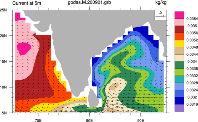
(b) salinity and current
(c) temperature
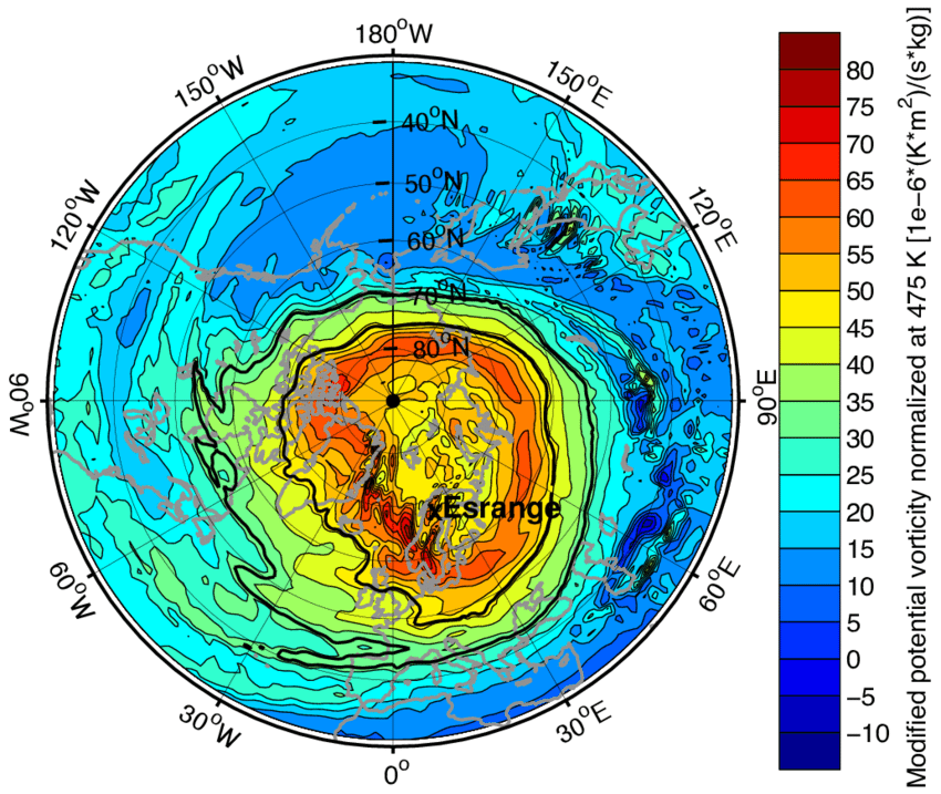
(d) vorticity
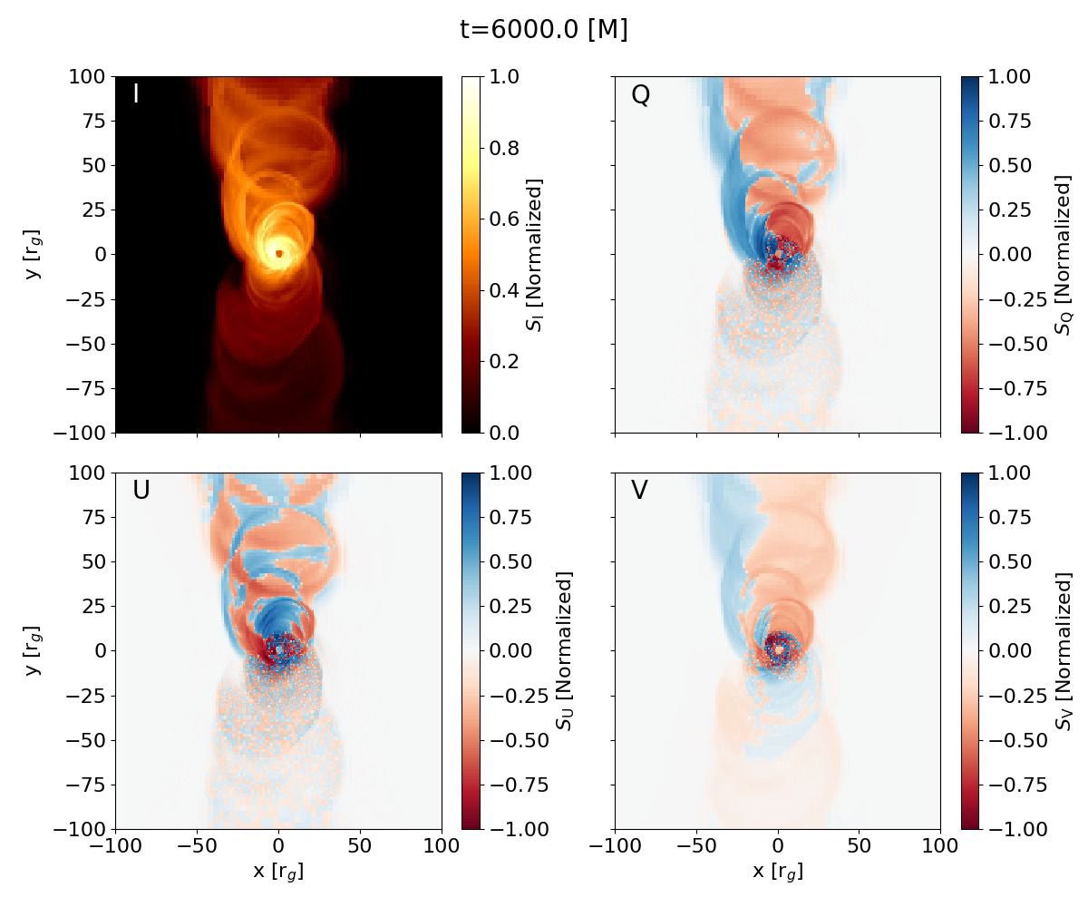
(e) intensity and polarization
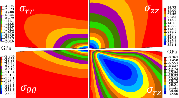
(f) stress tensor

Figure 1: Examples of geometric images in the natural sciences. (a) A visualization of a temperature map and a polarization map from the ESA Planck Mission [9]. The color map shows a temperature field (a scalar or ${0}_{(+)}$-tensor) on the sphere, and the whiskers show the principal eigenvector direction of a ${2}_{(+)}$-tensor field in two dimensions. In detail the underlying data are represented on a pixel grid (healpixel [22]) on the sky (a 2-sphere). (b) Two-dimensional maps of ocean current (shown with arrows; a vector or ${1}_{(+)}$-tensor field) and ocean salinity (shown with color; a scalar or ${0}_{(+)}$-tensor field) at a depth of 5 m [1]. (c) A three-dimensional map of temperature (a scalar or ${0}_{(+)}$-tensor field) based on sensors distributed throughout the volume of a granary [46]. (d) A two-dimensional map of potential vorticity (a pseudoscalar or ${0}_{(-)}$-tensor field) in the Earth’s atmosphere, measured for the purposes of predicting storms [34]. (e) Two-dimensional maps on the sky of intensity $I$ and the three independent components $Q,U,V$ of the electromagnetic polarization ${2}_{(+)}$-tensor, from a simulation of a jet outflow from an accreting black hole [Davelaar et al, in preparation]. (f) Components of the three-dimensional stress tensor (a ${2}_{(+)}$-tensor field) in a diamond anvil cell, which is used to study the behavior of samples at exceedingly high pressures [33].

At the present day, the go-to tools for machine learning with images are convolutional neural networks (CNNs; [32]) and their many descendants, including residual networks (ResNets) [25], dense networks (DenseNets)[26], and attention mechanisms such as transformers [43]. Other recent tools for machine learning with images include generative adversarial networks (GANs)[19] for image synthesis and style transfer, and recurrent neural networks (RNNs)[40] for tasks such as image captioning and video analysis. Additionally, transfer learning [54] has emerged as a powerful technique for leveraging pre-trained models on large image datasets to improve performance on smaller or specialized datasets.

Traditional CNNs are designed to work on one- or few-channel images in which the early layers of the network involve image convolutions with learned filters followed by the application of pointwise nonlinearities. In typical contexts, the channels of multi-channel input images will be something like the red, green, and blue channels of a color image; these can be combined arbitrarily in the layers of the CNN. When these CNN-based tools are applied to lattices of vectors, typically the components of the vectors are just treated as channels of the input image and then everything proceeds as with multi-channel color images. This ignores the inherent structure of the vectors, but, to the chagrin of the physicists, there are many projects that have had great success using this strategy on geometric images. However, there are better choices. Here we propose a set of tools that generalize the concept of convolution to apply to geometric images such that the outputs of the convolutions are also geometric images, obeying the same geometric transformation rules as the inputs.

The fundamental observation inspiring this work is that when an arbitrary function is applied to the components of vectors and tensors, the geometric structure of these objects is destroyed. There are strict rules, dating back to the early days of differential geometry [39], about how geometric objects can be combined to produce new geometric objects, consistent with coordinate freedom and transformation rules. These rules constitute a theme of [41], where they are combined into a geometric principle. In previous work [44, 45, 52] we have capitalized on the geometric principle to develop modified machine-learning methods that are restricted to exactly obey group-theoretic equivariances in physics contexts. More broadly there is a growing field of physics informed machine learning [29, 37]. Here we use these rules to create a comprehensive set of tools that parameterize functions that take geometric images as input and produce geometric images as output.

Tensors can be defined—and distinguished from mere arrays of numbers—in two ways. In one, a tensor of order $k$ is a $k$-multilinear function of $k$ vector inputs that returns a scalar, an object whose value is invariant to changes in the coordinate system ([41] Section 1.3). In the other, a tensor of order $k$ is defined by the way that its components transform under rotations ([41] Section 1.6). We will take the latter point of view, and this definition will be made precise in Section 2.1.

There are two ways to think about transformations—alias and alibi. In the former (alias), the idea is that the transformation is applied to the coordinate system, not the vectors and tensors themselves. This transformation leaves the geometric objects unchanged but all of their components change because they are now being represented in a changed coordinate system. In the latter (alibi), the idea is that the coordinate system is fixed and all of the geometric objects are taken through an identical transformation. In either case—alias or alibi—the key idea is that all of the components of all of the vectors and tensors in play must be changed correspondingly, and at the same time. The geometric principle requires that for any function, all the inputs, constants, parameters, and outputs must undergo the same coordinate transformations simultaneously. In other words, all valid functions will be fundamentally equivariant with respect to coordinate transformations.

We are motivated in this work to help solve problems in the natural sciences and engineering, where geometric images abound. However, we conjecture that these tools are probably very useful even for standard machine-learning image-recognition and image-regression tasks. After all, even standard images are measurements of a scalar, the intensity of light, at a regular grid of points on a two-dimensional surface. The laws of physics still govern the objects in a photograph and how light travels from the objects to the camera, so we may still expect to benefit from the rules of geometry.

These rules of geometry—the consequences of the geometric principle—are roughly as follows: A $k$-tensor object (tensor of order $k$) in $d$ dimensions has $k$ indices, each of which can take a value from 1 to $d$; that is, the $k$-tensor is an element of $(\mathbb{R}^{d})^{\otimes k}$. A $k$-tensor and a $k^{\prime}$-tensor can be multiplied with the outer product to make a $(k+k^{\prime})$-tensor object. To reduce the tensor order, a $k$-tensor can be contracted to a $(k-2)$-tensor object by identifying a pair of indices and summing over them. $1$-tensor objects are called vectors and $0$-tensor objects are called scalars. There are also negative-parity versions of all these (pseudoscalars, pseudovectors, and pseudotensors) and parity-changing contractions using the Levi-Civita symbol, so in what follows we will define ${k}_{(p)}$-tensors that have $k$ indices and a parity $p\in\{-1,+1\}$ (sometimes denoted “$-$” and “$+$” below). Two objects can only be added or subtracted if they have the same order $k$ and parity $p$. These rules define objects that can be given transformation rules under rotation and reflection such that functions made of these operations are coordinate-free, or equivariant to any change of coordinate system.

The symmetries that suggest these rules are continuous symmetries. But of course images are usually—and for our purposes—discrete grids of values. This suggests that in addition to the continuous symmetries respected by the tensor objects in the image pixels there will be discrete symmetries for each geometric image taken as a whole. We will define these discrete symmetry groups and use them to define a useful kind of group equivariance for functions of geometric images. This equivariance, it turns out, is very easy to enforce, even for nonlinear functions of geometric images, provided that we compose our nonlinear functions from simple geometric operations. When we enforce this equivariance, the convolution filters that appear look very much like the differential operators that appear in discretizations of vector calculus.

Our contribution:

The rest of the paper is organized in the following manner. Section 2 defines geometric objects, geometric images, and the operations on each. Section 3 discusses equivariance of functions of geometric images with some important results building off of [30] and [7]. Section 4 describes how to explicitly count these equivariant functions using a result of Molien from 1897. Sections 5 and 6 describe how to build a GeometricImageNet and present a couple of small problems with numerical results. Finally, Section 7 discusses related work. The majority of the supporting propositions and proofs have been sequestered to the Appendix, as has a larger exploration of related work.

Section 2 Geometric Objects and Geometric Images

We define the geometric objects and geometric images that we use to generalize classical images in scientific contexts in Section 2.1 and Section 2.2. The main point is that the channels of geometric images—which will be like the components of vectors and tensors—are not independent. There is a set of allowed operations on geometric objects that respect the structure and the coordinate freedom of these objects.

2.1 Geometric objects

The geometric principle implies that geometric objects should be coordinate-free scalars, vectors, and tensors, or their negative-parity pseudo counterparts. To define these objects we start by stating the coordinate transformations, which, in this case, will be given by the orthogonal group.

We fix $d$, the dimension of the space, which will typically be 2 or 3. The geometric objects are vectors and tensors. The orthogonal group $O(d)$ is the space of isometries of $\mathbb{R}^{d}$ that fix the origin. It acts on vectors and pseudovectors $v\in\mathbb{R}^{d}$ in the following way:

$$g\cdot v=\det(M(g))^{\frac{1-p}{2}}\,M(g)\,v$$ (1)

where for $g\in O(d)$, $M(g)\in\mathbb{R}^{d\times d}$ is the standard matrix representation of $g$ (i.e. $M(g)^{\top}\,M(g)=I$) and $p\in\{-1,+1\}$ is the parity of $v$. If $p=+1$ we obtain the standard $O(d)$ action on $\mathbb{R}^{d}$ vectors. If $p=-1$ we obtain the $O(d)$ action on what in physics are known as pseudovectors.

The objects are defined by the actions that they carry in the following sense: if $F$ is a function with geometric inputs, outputs, and parameters, then $F$ must be coordinate-free. In other words $F(g\cdot v)=g\cdot F(v)$ for all $v$ and all $g$. This is the mathematical concept of equivariance which we will explore further in Section 3.

Definition 1 (${k}_{(p)}$-tensors).

The space $\mathbb{R}^{d}$ equipped with the action $O(d)$ defined by (1) is the space of ${1}_{(p)}$-tensors. If $v_{i}$ is a ${1}_{(p_{i})}$-tensor, then $T:=v_{1}\otimes\ldots\otimes v_{k}$ is a rank-1 ${k}_{(p)}$-tensor, where $p=\prod_{i=1}^{k}p_{i}$ and the action of $O(d)$ is defined as

$$g\cdot(v_{1}\otimes\ldots\otimes v_{k})=(g\cdot v_{1})\otimes\ldots\otimes(g\cdot v_{k})~{}.$$ (2)

Higher rank ${k}_{(p)}$-tensors are defined as linear combinations of rank-1 ${k}_{(p)}$-tensors where the action of $O(d)$ is extended linearly. The set of ${k}_{(p)}$-tensors in $d$ dimensions is denoted $\mathcal{T}_{d,k,p}$.

Remark (terminology and notation).

The parity $p$ is a signed bit, either $+1$ for positive parity or $-1$ for negative parity. Note the distinction between the order $k$ of the ${k}_{(p)}$-tensor, and the rank of the tensor. We could have a ${2}_{(p)}$-tensor of rank 1, like those we use in Definition 1.

Remark (universality of transformations).

Critically, when a transformation is applied to any ${k}_{(p)}$-tensor, it must be applied to every other geometric object—every scalar, vector, and tensor of both parities—involved in any relevant mathematical expression. This includes all constants, and all inputs and outputs to any scalar, vector, or tensor functions. Related to this, there are both alias and alibi points of view that can be taken towards (2); that is, it can be seen as defining a change made to every tensor in a fixed coordinate system, or it can be seen as a change to the coordinate system in which every tensor is represented.

In physics the ${1}_{(+)}$-tensors (such as velocities) are known as vectors, the ${1}_{(-)}$-tensors (such as angular momenta) are known as pseudovectors, the ${0}_{(+)}$-tensors (such as rest masses) are known as scalars, the ${0}_{(-)}$-tensors (such as surface vorticities) are known as pseudoscalars, the ${k}_{(-)}$-tensors with $k\geq 2$ are known as pseudotensors, and finally the ${k}_{(+)}$-tensors with $k\geq 2$ are the things that are commonly known as tensors. In general, any ${k}_{(p)}$-tensor can be written as a sum of outer products of order-1 tensors (vectors and pseudovectors), where each term in the sum is an outer product of $k$ order-$1$ tensors and the parity $p$ is the product of the parities of the input order-$1$ tensors.

Definition 2 (outer products of tensors).

Given $a\in\mathcal{T}_{d,k,p}$ and $b\in\mathcal{T}_{d,k^{\prime},p^{\prime}}$, the outer product, denoted $a\otimes b$, is a tensor in $\mathcal{T}_{d,k+k^{\prime},p\,p^{\prime}}$ defined as $[a\otimes b]_{i_{1},\ldots,i_{k+k^{\prime}}}=[a]_{i_{1},\ldots,i_{k}}\,[b]_{i_{k+1},\ldots,i_{k+k^{\prime}}}$.

Definition 3 (Einstein summation notation).

We use Einstein summation notation where outer products are written in component form, and repeated indices are summed over. For example, in this notation, the product of two ${2}_{(+)}$-tensors (represented as two $d\times d$ matrices $A$ and $B$) is written as

$$[A\,B]_{i,j}=[A]_{i,k}\,[B]_{k,j}:=\sum_{k=1}^{d}[A]_{i,k}\,[B]_{k,j}$$ (3)

where $[A]_{i,k}$ is the $i,k$ element of matrix $A$, and the sum from 1 to $d$ on repeated index $k$ is implicit in the middle expression. This notation works for tensor expressions of any order, provided that every index appears either exactly once, so it isn’t summed over, or exactly twice, so it is summed over.

Remark (lower and upper indices).

In the original Einstein summation notation [14], or Ricci calculus [39], a distinction is made between lower and upper indices, which correspond to covariant and contravariant components. The pairs of indices that are summed always have one member of the pair an upper index and one member a lower index. We drop the upper/lower distinction here because we will work with intrinsically flat images that implicitly have the Riemmannian metric given by the identity matrix, such that there is no numerical difference between covariant and contravariant component values for a given object. That said, there truly is a distinction (for example, if a spatial displacement is a contravariant vector, the gradient of a scalar function with respect to that spatial displacement is a covariant vector), so there might be advantages to reinstating this distinction.

In summation notation, the group action of (1) on ${k}_{(p)}$-tensor $b$ is explicitly written

$$[g\cdot b]_{i_{1},\ldots,i_{k}}=\det(M(g))^{\frac{1-p}{2}}\,[b]_{j_{1},\ldots,j_{k}}\,[M(g)]_{i_{1},j_{1}}\cdots[M(g)]_{i_{k},j_{k}}$$ (4)

for all $g\in O(d)$, where $[b]_{i_{1},\ldots,i_{k}}\in\mathbb{R}$ is a component of $b$, $[M(g)]_{i,j}\in\mathbb{R}$ is the $i,j$ element of the matrix representation of $g$, and all the $i_{m}$ and $j_{m}$ are indices in the range $1,\ldots,d$. For example, a ${2}_{(+)}$-tensor has the transformation property $[g\cdot b]_{i,j}=[b]_{k,\ell}\,[M(g)]_{i,k}\,[M(g)]_{j,\ell}$, which, in normal matrix notation, is written as $g\cdot b=M(g)\,b\,M(g)^{\top}$.

We consider two special tensors that will be important for the definition of our models, the Kronecker delta and the Levi-Civita symbol.

Definition 4 (Kronecker delta).

The Kronecker delta, $\delta$, is a ${2}_{(+)}$-tensor represented by the identity matrix, namely the object with two indices $i,j$ such that it has the value $+1$ when the two indices have the same value ($i=j$), and $0$ otherwise.

Definition 5 (Levi-Civita symbol).

The Levi-Civita symbol in dimension $d\geq 2$ is a ${d}_{(-)}$-tensor $\epsilon$ such that if the $d$ indices are not repeated and in an even-permutation order the value is $+1$ and if the $d$ indices are not repeated and in an odd-permutation order the value is $-1$, and it has the value $0$ in all other cases.

Definition 6 (contractions).

Given tensor $a\in\mathcal{T}_{d,k,p}$, where $k\geq 2$, and given $\mu,\nu\in[k],\mu\not=\nu$, the contraction $T(a,\mu,\nu)\in\mathcal{T}_{d,k-2,p}$ is defined as:

$$[T(a,\mu,\nu)]_{i_{1},\ldots,i_{k}\setminus\quantity{i_{\mu},i_{\nu}}}=[\delta]_{i_{\mu}i_{\nu}}\,[a]_{i_{1},\ldots,i_{\mu},\ldots,i_{\nu},\ldots,i_{k}}$$ (5)

That is, we view the components of $a$ with given fixed values for $i_{\mu}$ and $i_{\nu}$ as forming a ${(k-2)}_{(p)}$-tensor, and then we take the sum of these tensors of order $k-2$ where $i_{\mu}=i_{\nu}$. We can also define the composition of multiple contractions as a multicontraction:

$$T_{M}(a,(\mu_{1},\mu_{2}),\ldots,(\mu_{\ell},\mu_{\ell+1}))=T(\cdot,\mu_{\ell},\mu_{\ell+1})\circ\ldots\circ T(a,\mu_{1},\mu_{2})~{},$$ (6)

where $\mu_{1},\ldots,\mu_{\ell+1}\in[k]$ are all distinct. Note that because $\mu_{1},\ldots,\mu_{\ell+1}$ are integers referring to the indices of the axes being contracted, the indices may change when swapping from a multicontraction to multiple contractions. For example, if $k\geq 4$,

$$T_{M}(a,(1,3),(2,4))=T(T(a,1,3),1,2)$$

because axes $i_{1}$ and $i_{3}$ will disappear, so $i_{2}$ becomes the new $i_{1}$ and $i_{4}$ becomes the new $i_{2}$. Finally, the Levi-Civita contraction is defined for $k\geq d-1$ and $\mu_{1},\ldots,\mu_{d-1}\in[k]$ distinct as the following:

$$T_{LC}(a,\mu_{1},\ldots,\mu_{d-1})=T_{M}(a\otimes\epsilon,(\mu_{1},k+1),\ldots,(\mu_{d-1},k+d-1))~{},$$ (7)

where $\epsilon$ is the Levi-Civita symbol.

Remark (negative-parity objects).

With a slight modification of the Levi-Civita contraction, there is an invertible function that converts any negative-parity object to a positive-parity object. Thus it is possible to work without negative-parity objects at all. We will use this idea to improve the efficiency of our algorithms for certain settings in Section 5.2. However, since negative-parity objects are important in physics and engineering (see Figure 1), we retain them in the model.

We can combine multiplication with Kronecker and Levi-Civita symbols with contractions to define relevant operations. For example the ${2}_{(+)}$-tensor formed by the outer product of ${1}_{(+)}$-tensors $a$ and $b$ can be contracted with the Kronecker delta to give the standard dot product $a^{\top}b=[a]_{i}\,[b]_{j}\,[\delta]_{ij}$, which is a ${0}_{(+)}$-tensor or scalar. For another example, the same ${2}_{(+)}$-tensor can (in $d=3$ dimensions) be contracted with the Levi-Civita symbol to give the standard cross product $[a\times b]_{k}=[a]_{i}\,[b]_{j}\,[\epsilon]_{ijk}$, which is a ${1}_{(-)}$-tensor or pseudovector.

Definition 7 (permutations of tensor indices).

Given $a\in\mathcal{T}_{d,k,p}$ and permutation $\sigma\in S_{k}$, the permutation of tensor indices of $a$ by $\sigma$, denoted $a^{\sigma}$, is:

$$[a^{\sigma}]_{i_{1},\ldots,i_{k}}:=[a]_{i_{\sigma^{-1}(1)},\ldots,i_{\sigma^{-1}(k)}}$$ (8)

Remark (tensors as linear functions).

There is an alternative definition of ${k}_{(p)}$-tensors in terms of geometric functions (see, for example, [41] chapter 1): A ${k}_{(+)}$-tensor can be thought of as representing a multilinear function of $k$ vectors (${1}_{(+)}$-tensors) that produces a scalar (${0}_{(+)}$-tensor) output. For example, if $A$ is a ${4}_{(+)}$-tensor, and $u,v,w,x$ are vectors (${1}_{(+)}$-tensors) then

$$\rho=[A]_{ijk\ell}\,[u]_{i}\,[v]_{j}\,[w]_{k}\,[x]_{\ell}$$ (9)

is a scalar (${0}_{(+)}$-tensor). ${k}_{(-)}$-tensors can be similarly defined in terms of input vectors and an output pseudoscalar.

2.2 Geometric images and operations

We will start by considering square (or cubic or hyper-cubic) images on a $d$-torus. We work on a $d$-torus to simplify the mathematical results; all the definitions and operations will be applicable with minor adjustments to rectangular, non-toroidal arrays as well. We consider an image $A$ in with $N$ equally spaced pixels in each dimension for $N^{d}$ pixels total. Each pixel contains a ${k}_{(p)}$-tensor where $k$ and $p$ are the same for each pixel. Let $\mathcal{T}_{d,k,p}$ be the set of ${k}_{(p)}$-tensors in $\mathbb{R}^{d}$. We define the geometric images as follows.

Definition 8 (geometric image).

A geometric image is a function $A:[N]^{d}\to\mathcal{T}_{d,k,p}$, where $[N]=\{0,1,\ldots,N-1\}$. The set of geometric images is denoted $\mathcal{A}_{N,d,k,p}$. We will also consider ${k}_{(p)}$-tensor images on the $d$-torus, where $[N]^{d}$ is given the algebraic structure of $(\mathbb{Z}/N\mathbb{Z})^{d}$. The pixel index of a geometric image, often $\bar{\imath}$, is naturally a ${1}_{(+)}$-tensor of length $d$.

Definition 9 (sums of images).

Given $A,B\in\mathcal{A}_{N,d,k,p}$, the sum $A+B\in\mathcal{A}_{N,d,k,p}$ is defined as

$$(A+B)(\bar{\imath})=A(\bar{\imath})+B(\bar{\imath})$$ (10)

for pixel $\,\bar{\imath}$. That is, the sums of geometric images are performed pixel-wise.

Definition 10 (scalar multiplication of images).

Given $A\in\mathcal{A}_{N,d,k,p}$ and $\alpha\in\mathbb{R}$, the scalar product $\alpha A$ is defined as

$$(\alpha A)(\bar{\imath})=\alpha A(\bar{\imath})~{}.$$ (11)

Similarly, we define contractions and permutations as applying an identical contraction or permutation to every pixel.

We now turn to the first major contribution of this paper, the generalization of convolution to take geometric images as inputs and return geometric images as outputs. The idea is that a geometric image of ${k}_{(p)}$-tensors is convolved with a geometric filter of ${k^{\prime}}_{(p^{\prime})}$-tensors to produce a geometric image that contains ${(k+k^{\prime})}_{(p\,p^{\prime})}$-tensors, where each pixel is a sum of outer products. These ${(k+k^{\prime})}_{(p\,p^{\prime})}$-tensors can then be contracted down to lower-order tensors using contractions (Definition 6). Note that the sidelength $M$ of the geometric filter can be any positive odd number, but typically it will be much smaller than the sidelength $N$ of the geometric image.

Definition 11 (geometric convolution).

Given $A\in\mathcal{A}_{N,d,k,p}$ on the $d$-torus, and $C\in\mathcal{A}_{M,d,k^{\prime},p^{\prime}}$ where $M=2m+1$ for some $m\in\mathbb{N}$, the geometric convolution $A\ast C$ is a ${(k+k^{\prime})}_{(p\,p^{\prime})}$-tensor image such that

$$(A\ast C)(\bar{\imath})=\sum_{\bar{a}\in[-m,m]^{d}}A(\bar{\imath}-\bar{a})\otimes C(\bar{a}+\bar{m})~{},$$ (12)

where $\bar{\imath}-\bar{a}$ is the translation of $\bar{\imath}$ by $\bar{a}$ on the $d$-torus pixel grid $(\mathbb{Z}/N\mathbb{Z})^{d}$. Additionally, $\bar{m}$ is the $d$ length ${1}_{(+)}$-tensor $[m,\ldots,m]^{T}$. For example, if $d=2$ and $\bar{a}=[0,0]^{T}$, then $\bar{a}+\bar{m}=[m,m]^{T}$, the center pixel of $C$ as we would expect.

This definition is on the torus, which we use to simplify the mathematical exposition. To define the convolution on $[N]^{d}$ instead of the torus, we can pad the image out with zero tensors of the corresponding order and parity. See Figure 2 for examples with a scalar and vector filter.

* = * =

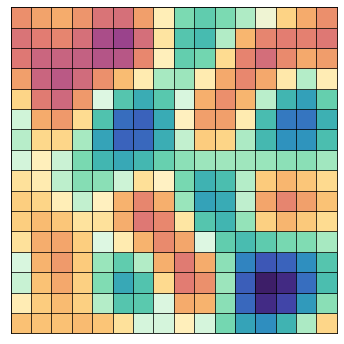
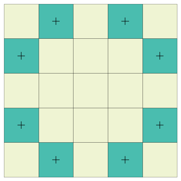
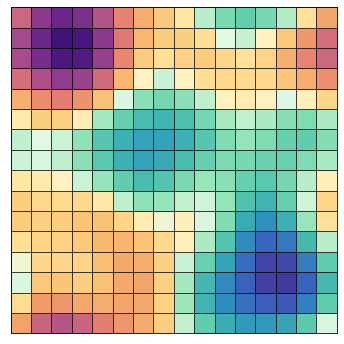
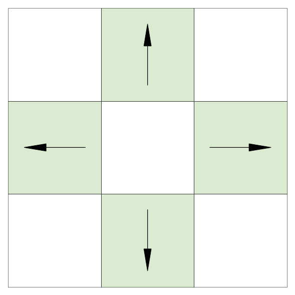
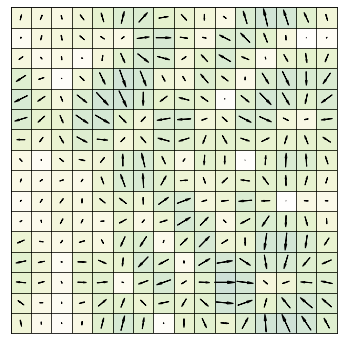
Figure 2: Convolution of a scalar image with a scalar filter and with a vector filter. Note that convolution with the vector filter results in a vector image that looks like the gradient.

In addition to contractions and index permutations that act pixel-wise in geometric images, it is possible to change the image size using pooling and unpooling operations. For both pooling and unpooling, there are alternative strategies to the ones we have defined below.

Definition 12 (average pooling).

Given $A\in\mathcal{A}_{N,d,k,p}$ and $b\in\mathbb{Z}^{+}$ such that $N$ is divisible by $b$, we define avg pool$(A,b)\in\mathcal{A}_{N/b,d,k,p}$ for pixel index $\bar{\imath}$ as:

$$\text{avg\,pool}(A,b)(\bar{\imath})=\frac{1}{b^{d}}\sum_{\bar{a}\in[0,b-1]^{d}}A(b\bar{\imath}+\bar{a})$$ (13)

Definition 13 (nearest neighbor unpooling).

Given $A\in\mathcal{A}_{N,d,k,p}$ and $b\in\mathbb{Z}^{+}$, we define unpool$(A,b)\in\mathcal{A}_{Nb,d,k,p}$ for pixel index $\bar{\imath}$ as:

$$\text{unpool}(A,b)(\bar{\imath})=A\quantity(\lfloor\bar{\imath}/b\rfloor)$$ (14)

where $\lfloor\bar{\imath}/b\rfloor$ denotes dividing each component of $\bar{\imath}$ by $b$, then taking element-wise floor operator of the resulting vector.

The convolution, contraction, index-permutation, and pooling operators above effectively span a large class of linear functions from geometric images to geometric images. One way to construct nonlinear functions is using polynomials, which in this context will be sums of outer products of any of the linear function outputs, possibly followed by further geometric convolutions and contractions. Nonlinear functions can also be constructed by applying nonlinear functions to ${0}_{(+)}$-tensors (scalars), or odd nonlinear functions to ${0}_{(-)}$-tensors (pseudoscalars); we will return to these methods in Section 5.

Definition 14 (outer products of images).

Given $A\in\mathcal{A}_{N,d,k,p}$ and $B\in\mathcal{A}_{N,d,k^{\prime},p^{\prime}}$, the outer product $A\otimes B\in\mathcal{A}_{N,d,k+k^{\prime},p\,p^{\prime}}$ is defined as

$$(A\otimes B)(\bar{\imath})=A(\bar{\imath})\otimes B(\bar{\imath})~{}.$$ (15)

for each pixel $\,\bar{\imath}$. That is, the outer products of geometric images are performed pixel-wise.

Section 3 Functions of geometric images and equivariance

We start by defining equivariance and invariance for a general group $G$, and then we will describe the groups of interest and several theoretical results.

Definition 15 (Equivariance of a geometric image function).

Given a function on geometric images $f:\mathcal{A}_{N,d,k,p}\to\mathcal{A}_{N,d,k^{\prime\prime},p^{\prime\prime}}$, and a group $G$ equipped with actions on $\mathcal{A}_{N,d,k,p}$ and $\mathcal{A}_{N,d,k^{\prime\prime},p^{\prime\prime}}$, we say that $f$ is equivariant to $G$ if for all $g\in G$ and $A\in\mathcal{A}_{N,d,k,p}$ we have:

$$f(g\cdot A)=g\cdot f(A)$$ (16)

Likewise, $f$ is invariant to $G$ if

$$f(g\cdot A)=f(A)~{}.$$ (17)

We may also say a geometric image is invariant to $G$ if $g\cdot A=A$ for all $g\in G$.

Convolutional filters are widely used in machine learning for scalar images. The fundamental property of these operators are that they are translation equivariant, and that every translation equivariant linear function can be expressed as a convolution with a fixed filter, as long as the filter can be set to be as large as the image. The same property holds for geometric images.

Definition 16 (Translation of ${k}_{(p)}$-tensor images).

Given a ${k}_{(p)}$-tensor image $A$ on the $d$-torus, and a translation $\tau\in(\mathbb{Z}/N\mathbb{Z})^{d}$, the action $L_{\tau}A$ produces a ${k}_{(p)}$-tensor image on the $d$-torus such that

$$(L_{\tau}A)(\bar{\imath})=A(\bar{\imath}-\tau)~{},$$ (18)

where $\bar{\imath}-\tau$ is the translation of $\bar{\imath}$ by $\tau$ on the $d$-torus pixel grid $(\mathbb{Z}/N\mathbb{Z})^{d}$.

Proposition 1.

A function $f:\mathcal{A}_{N,d,k,p}\to\mathcal{A}_{N,d,k+k^{\prime},p\,p^{\prime}}$ is a translation equivariant linear function if and only if it is the convolution with a geometric filter $C\in\mathcal{A}_{M,d,2k+k^{\prime},p^{\prime}}$ followed by $k$ contractions. When $N$ is odd, $M=N$, otherwise $M=N+1$.

Note that this proposition merely generalizes the result of [30] for geometric convolution when the group is discrete translations. See appendix A for the proof.

In addition to translation symmetries, we want to consider other natural symmetries occurring in the application domains where vectors and tensors arise. Ideally we would like to apply continuous rotations to the images, but the discretized nature of images makes this challenging. For simplicity, we focus on discrete rotations, and we extend the group action to the geometric objects in these images.

Definition 17 (Group $B_{d}$ of symmetries of a $d$-hypercube).

We denote by $B_{d}$ the group of Euclidean symmetries of the $d$-dimensional hypercube.

The group $B_{d}$ is often called the hyperoctahedral group since the $d$-dimensional hyperoctahedron is dual to the hypercube, so they have the same group of symmetries. The notation $B_{d}$ is standard nomenclature coming from the classification theorem for finite irreducible reflection groups [27]. See Figure 3 for a depiction of the elements of $B_{2}$ acting on a vector. Because the groups $B_{d}$ are subgroups of $O(d)$, all determinants of the matrix representations of the group elements are either $+1$ or $-1$, and the matrix representation $M(g^{-1})$ of the inverse $g^{-1}$ of group element $g$ is the transpose of the matrix representation $M(g)$ of group element $g$.

Definition 18 (Action of $B_{d}$ on ${k}_{(p)}$-tensors).

Given a ${k}_{(p)}$-tensor $b$, the action of $g\in B_{d}$ on $b$, denoted $g\cdot b$, is the restriction of the action in Definition 1 to $B_{d}$ which is a subgroup of $O(d)$.

Definition 19 (Action of $B_{d}$ on ${k}_{(p)}$-tensor images).

Given $A\in\mathcal{A}_{N,d,k,p}$ on the $d$-torus and a group element $g\in B_{d}$, the action $g\cdot A$ produces a ${k}_{(p)}$-tensor image on the $d$-torus such that

$$(g\cdot A)(\bar{\imath})=g\cdot A({g^{-1}\cdot\bar{\imath}})~{}.$$ (19)

Since $\bar{\imath}$ is a ${1}_{(+)}$-tensor, the action $g^{-1}\cdot\bar{\imath}$ is performed by centering $\bar{\imath}$, applying the operator, then un-centering the pixel index:

$$g^{-1}\cdot\bar{\imath}=\quantity(M(g^{-1})(\bar{\imath}-\bar{m}))+\bar{m}$$

where $\bar{m}$ is the $d$-length ${1}_{(+)}$-tensor $\quantity[\frac{N-1}{2},\ldots,\frac{N-1}{2}]^{T}$. If the pixel index is already centered, such as $\bar{a}\in[-m,m]^{d}$, then we skip the centering and un-centering.

It might be a bit surprising that the group element $g^{-1}$ appears in the definition of the action of the group on images. One way to think about it is that the pixels in the transformed image are “looked up” or “read out” from the pixels in the original untransformed image. The pixel locations in the original image are found by going back, or inverting the transformation.

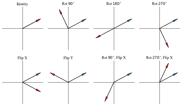
Figure 3: The elements of $B_{2}$ on the vector $\matrixquantity[2\\ 1]$. The original vector is blue and the transformed vector is red. Rotations are in degrees counterclockwise, flips are over the axis specified. The group $B_{d}$ has $d!2^{d}$ elements, so $d=3$ has $48$ and $d=4$ has 384 elements.

Definition 20 (The group $G_{N,d}$, and its action on ${k}_{(p)}$-tensor images).

$G_{N,d}$ is the group generated by the elements of $B_{d}$ and the discrete translations on the $N^{d}$-pixel lattice on the $d$-torus.

Remark.

We view the $d$-torus as the quotient of the $d$-hypercube obtained by identifying opposite faces. The torus obtains the structure of a flat (i.e., zero curvature) Riemannian manifold this way. Because the symmetries $B_{d}$ of the hypercube preserve pairs of opposite faces, they act in a well-defined way on this quotient, so we can also view $B_{d}$ as a group of isometries of the torus. We choose the common fixed point of the elements of $B_{d}$ as the origin for the sake of identifying the $N^{d}$ pixel lattice with the group $T_{N,d}\cong(\mathbb{Z}/N\mathbb{Z})^{d}$ of discrete translations of this lattice; then the action of $B_{d}$ on the torus induces an action of $B_{d}$ on $T_{N,d}$ by automorphisms. The group $G_{N,d}$ is the semidirect product $T_{N,d}\rtimes B_{d}$ with respect to this action. Thus there is a canonical group homomorphism $G_{N,d}\rightarrow B_{d}$ with kernel $T_{N,d}$. In concrete terms, every element of $G_{N,d}$ can be written in the form $\tau\circ b$, where $b\in B_{d}$ and $\tau\in T_{N,d}$. Then the canonical map $G_{N,d}\rightarrow B_{d}$ sends $\tau\circ b$ to $b$.

Now that we have defined the group that we are working with, we can specify how to build convolution functions that are equivariant to $G_{N,d}$. The following theorem generalizes the Cohen and Welling paper [7] for geometric convolutions.

Theorem 1.

A ${k^{\prime}}_{(p^{\prime})}$-tensor convolution filter $C$ produces convolutions that are equivariant with respect to the big group $G_{N,d}$ if $C$ is invariant under the small group $B_{d}$.

To prove this, we will first state and prove a key lemma.

Lemma 1.

Given $g\in B_{d}$, $A\in\mathcal{A}_{N,d,k,p},$ and $C\in\mathcal{A}_{M,d,k^{\prime},p^{\prime}}$, the action $g$ distributes over the convolution of $A$ with $C$:

$$g\cdot(A*C)=(g\cdot A)*(g\cdot C)$$ (20)

Proof.

Let $A\in\mathcal{A}_{N,d,k,p}$ be a geometric image, let $C\in\mathcal{A}_{M,d,k^{\prime},p^{\prime}}$, let $g\in B_{d}$, and let $\bar{\imath}$ be any pixel index of $A$. By Definition 19 we have

$$(g\cdot(A*C))\quantity(\bar{\imath}) =g\cdot\quantity((A*C)\quantity(g^{-1}\cdot\bar{\imath}))$$

$$=g\cdot\quantity(\sum_{\bar{a}\in[-m,m]^{d}}A\quantity(g^{-1}\cdot\bar{\imath}-\bar{a})\otimes C\quantity(\bar{a}+\bar{m}))$$

$$=\sum_{\bar{a}\in[-m,m]^{d}}g\cdot\quantity(A\quantity(g^{-1}\cdot\bar{\imath}-\bar{a})\otimes C\quantity(\bar{a}+\bar{m}))$$

$$=\sum_{\bar{a}\in[-m,m]^{d}}g\cdot A\quantity(g^{-1}\cdot\bar{\imath}-\bar{a})\otimes g\cdot C\quantity(\bar{a}+\bar{m})$$

Now let $\bar{a}^{\prime}=g\cdot\bar{a}$. Thus $g^{-1}\cdot\bar{a}^{\prime}=g^{-1}\cdot g\cdot\bar{a}=\bar{a}$. Then:

$$(g\cdot(A*C))(\bar{\imath}) =\sum_{\bar{a}\in[-m,m]^{d}}g\cdot A\quantity(g^{-1}\cdot\bar{\imath}-\bar{a})\otimes g\cdot C\quantity(\bar{a}+\bar{m})$$

$$=\sum_{g^{-1}\cdot\bar{a}^{\prime}\in[-m,m]^{d}}g\cdot A\quantity(g^{-1}\cdot\bar{\imath}-g^{-1}\cdot\bar{a}^{\prime})\otimes g\cdot C\quantity(g^{-1}\cdot\bar{a}^{\prime}+\bar{m})$$

$$=\sum_{g^{-1}\cdot\bar{a}^{\prime}\in[-m,m]^{d}}g\cdot A\quantity(g^{-1}\cdot\bar{\imath}-g^{-1}\cdot\bar{a}^{\prime})\otimes g\cdot C\quantity(g^{-1}\cdot\bar{a}^{\prime}+g^{-1}\cdot\bar{m})$$

$$=\sum_{g^{-1}\cdot\bar{a}^{\prime}\in[-m,m]^{d}}g\cdot A\quantity(g^{-1}\cdot\quantity(\bar{\imath}-\bar{a}^{\prime}))\otimes g\cdot C\quantity(g^{-1}\cdot\quantity(\bar{a}^{\prime}+\bar{m}))$$

$$=\sum_{g^{-1}\cdot\bar{a}^{\prime}\in[-m,m]^{d}}\quantity(g\cdot A)\quantity(\bar{\imath}-\bar{a}^{\prime})\otimes\quantity(g\cdot C)\quantity(\bar{a}^{\prime}+\bar{m})$$

$$=\sum_{\bar{a}^{\prime}\in[-m,m]^{d}}\quantity(g\cdot A)\quantity(\bar{\imath}-\bar{a}^{\prime})\otimes\quantity(g\cdot C)\quantity(\bar{a}^{\prime}+\bar{m})$$

$$=\quantity((g\cdot A)*(g\cdot C))(\bar{\imath})$$

For the penultimate step, we note that $g^{-1}\cdot\bar{a}^{\prime}\in[-m,m]^{d}$ compared to $\bar{a}^{\prime}\in[-m,m]^{d}$ is just a reordering of those indices in the sum. Thus we have our result for pixel $\bar{\imath}$, so it holds for all pixels. ∎

With this lemma, the proof of Theorem 1 follows quickly.

Proof of Theorem 1.

Let $A\in\mathcal{A}_{N,d,k,p}$ be a geometric image and let $C\in\mathcal{A}_{M,d,k^{\prime},p^{\prime}}$ be a convolution filter invariant to $B_{d}$. It is well known that convolution is equivariant to translations, and we prove it again the appendix for our definition of convolution (32). Now suppose $g\in B_{d}$. By Lemma 1 and the $B_{d}$-invariance of $C$ we have:

$$g\cdot(A*C)=(g\cdot A)*(g\cdot C)=(g\cdot A)*C$$

Thus the convolution is equivariant to the generators of $G_{N,d}$, so it is equivariant to the group. ∎

Theorem 1 provides the foundation for building our equivariant GeometricImageNet. Finding the set of $B_{d}$-invariant ${k^{\prime}}_{(p^{\prime})}$-tensor filters is straightforward using group averaging – see Section 5 for implementation details. See Figure 4 and Figure 5 for the invariant convolutional filters in $d=2$ dimensions for filters of sidelength $M=3$ and $M=5$ respectively. We now show some important relationships between the invariant filters of different tensor orders and parities.

Proposition 2.

Let $C\in\mathcal{A}_{M,d,k^{\prime},p^{\prime}}$ be a $B_{d}$-invariant convolutional filter and let $\Delta\in\mathcal{A}_{M,d,2,+}$ be the geometric image with the Kronecker delta, $\delta$, in every pixel. Then $C\otimes\Delta\in\mathcal{A}_{M,d,k^{\prime}+2,p^{\prime}}$ is a $B_{d}$-invariant convolutional filter.

Proof.

This proof follows quickly from the $B_{d}$-invariance of the Kronecker delta, which holds because $B_{d}\subset O(d)$ (see Proposition 6 in the Appendix). With $C$ and $\Delta$ defined as above and pixel index $\bar{\imath}$, we have:

$$(g\cdot(C\otimes\Delta))(\bar{\imath}) =(g\cdot C\otimes g\cdot\Delta)(\bar{\imath})$$

$$=(g\cdot C)(\bar{\imath})\otimes(g\cdot\Delta)(\bar{\imath})$$

$$=C(\bar{\imath})\otimes g\cdot\Delta(g^{-1}\cdot\bar{\imath})$$

$$=C(\bar{\imath})\otimes g\cdot\delta$$

$$=C(\bar{\imath})\otimes\delta$$

$$=C(\bar{\imath})\otimes\Delta(\bar{\imath})$$

$$=(C\otimes\Delta)(\bar{\imath})$$

∎

Proposition 3.

Let $C\in\mathcal{A}_{M,d,k^{\prime},p^{\prime}},k^{\prime}\geq d-1$ be a $B_{d}$-invariant convolutional filter and $\mu_{1},\ldots,\mu_{d-1}\in[k^{\prime}]$ distinct. Then $T_{LC}(C,\mu_{1},\ldots,\mu_{d-1})\in\mathcal{A}_{M,d,k^{\prime}-d+2,-p^{\prime}}$ is a $B_{d}$-invariant filter of opposite parity of $C$.

Proof.

Let $C$ and $\mu_{1},\ldots,\mu_{d-1}$ be defined as above and let $g\in B_{d}$. We can immediately see that $T_{LC}(C,\mu_{1},\ldots,\mu_{d-1})$ is $B_{d}$-invariant by the equivariance of the Levi-Civita contraction (43), so

$$g\cdot T_{LC}(C,\mu_{1},\ldots,\mu_{d-1})=T_{LC}(g\cdot C,\mu_{1},\ldots,\mu_{d-1})=T_{LC}(C,\mu_{1},\ldots,\mu_{d-1})~{}.$$

Thus we just have to verify that $T_{LC}(C,\mu_{1},\ldots,\mu_{d-1})\in\mathcal{A}_{M,d,k^{\prime}-d+2,-p^{\prime}}$. Since the outer product adds tensor orders and multiplies parities, at each pixel $\bar{\imath},C(\bar{\imath})\otimes\epsilon\in\mathcal{T}_{d,k^{\prime}+d,-p^{\prime}}$. Performing $d-1$ contractions reduces the tensor order by $2(d-1)$, so the resulting tensor order is $k^{\prime}+d-2(d-1)=k^{\prime}+d-2d+2=k^{\prime}-d+2$ as desired. ∎

The consequence of Propositions 2 and 3 is a natural pairing between $B_{d}$-invariant convolutional filters. See the caption of Figure 4 for further details. In practice, this allows us to dramatically reduce the number of filters we need to use in certain applications, as we will explore in Section 5.2.

Figure 4: All the filters for $d=2$, $M=3$, $k^{\prime}\in[0,1,2]$. Notes: Scalars and pseudo-scalars are shown with signed colors; where there is no symbol in the box the value is zero. The ${2}_{(p^{\prime})}$-tensor filters are shown via the action of the tensor on an image of a letter “R”; the transformation properties of the ${2}_{(p^{\prime})}$-tensor filters are such that these filters may not look obviously invariant to rotations. There are no invariant pseudoscalar (${0}_{(-)}$-tensor) filters available at $d=2,M=3$. Note that scalar 0 and scalar 2 are paired with ${2}_{(+)}$-tensor 0 and ${2}_{(+)}$-tensor 3 respectively by multiplication with the Kronecker delta symbol, per Proposition 2. Likewise, if we added ${2}_{(+)}$-tensor 1 and ${2}_{(+)}$-tensor 2 together, they would be paired with scalar 1. Also note that each ${1}_{(+)}$-tensor filter is paired with a ${1}_{(-)}$-tensor filter and likewise for each ${2}_{(+)}$-tensor filter and ${2}_{(-)}$-tensor filter by Proposition 3. We don’t show the ${k^{\prime}}_{(p^{\prime})}$-tensor filters at $k^{\prime}>2$ because visualizing them is difficult, even the $k^{\prime}=2$ case is potentially misleading. Note that the vector (${1}_{(+)}$-tensor) filters look like pure divergence and the pseudovector (${1}_{(-)}$-tensor) filters look like pure curl.

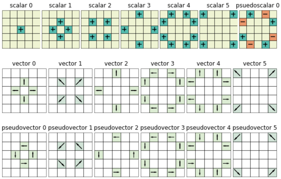
Figure 5: All the filters for $d=2$, $M=5$, $k^{\prime}\in[0,1]$. The symbols and colors are as in Figure 4. We don’t show the ${2}_{(p^{\prime})}$-tensor filters at $m=2$ because there are 26 of them. At $(d,m)=(2,2)$ a pseudoscalar filter appears. Again, the vector and pseudovectors look like pure divergence and pure curl, respectively.

Section 4 Counting equivariant maps

With an eye to understanding the expressive power of convolution-based functions, we show how to compute the dimension of the vector space of equivariant polynomial maps of given degree.

Suppose a finite group $G$ acts on a pair of real vector spaces $V$ and $W$. Let $\mathcal{F}$ be the collection of all equivariant polynomial maps $V\to W$, and let $\mathcal{F}_{\ell}\subseteq\mathcal{F}$ be the homogeneous equivariant polynomials of degree $\ell$. The set $\mathcal{F}_{\ell}$ forms a finite-dimensional real vector space whose dimension is dependent on $\ell$. Thus $\dim\quantity(\mathcal{F}_{\ell})$ forms a nonnegative integer sequence indexed by $\ell=0,1,2,\dots$. The generating function of this sequence,

$$H\quantity(\mathcal{F},t):=\sum_{\ell\geq 0}\dim\quantity(\mathcal{F}_{\ell})\,t^{\ell}~{},$$ (21)

is known as the Hilbert series of our set of functions. A variant [11, Remark 3.4.3] on a classical result known as Molien’s theorem expresses this generating function as a finite sum of explicit rational functions:

$$H(\mathcal{F},t)=\frac{1}{|G|}\sum_{g\in G}\frac{\tr\quantity(M_{W}\quantity(g^{-1}))}{\det(I-M_{V}(g)\,t)}~{},$$ (22)

where $M_{V}(g),M_{W}(g^{-1})$ are matrices describing the actions of $g,g^{-1}$ on $V,W$ respectively. The trace in the numerator is also known as the character of $W$ evaluated at $g^{-1}$.

Remark.

The set $\mathcal{F}$ is also known as the module of covariants and written $(\mathbb{R}[V]\otimes W)^{G}$, or $\operatorname{Mor}_{G}(V,W)$, or $\operatorname{Mor}(V,W)^{G}$. In this context, the word module refers to the fact that the set of equivariant polynomial maps is closed under multiplication by arbitrary $G$-invariant polynomial functions on $V$ as well as closed under addition. Covariant is another word for equivariant map, coming from classical invariant theory.

The right side of (22) is reasonable to compute in practice. To illustrate, we compute it for the group $G_{N,2}$ of Definition 20, with $V=W=\mathcal{A}_{N,2,1,+}$, the space of $2$-dimensional geometric images whose pixels consist of vectors. We assume $N$ is odd.

We first compute the character $\tr\quantity(M(g))$ for $g\in G_{N,2}$. This can be done explicitly by writing down a basis for $\mathcal{A}_{N,2,1,+}$ and expressing the action of each element of $G_{N,2}$ in terms of that basis. The computation is expedited by the choice of a basis in which the action of $G_{N,2}$ is monomial, that is, for basis vector $e_{i}$ and any $g\in G_{N,d}$, we have $g\cdot e_{i}=\alpha\,e_{j}$, where $\alpha\in\mathbb{R}$ and $e_{j}$ is some basis vector which may be the same as $e_{i}$. When this condition holds, only the basis eigenvectors contribute to the trace. The group $B_{2}$ acts monomially on the standard basis vectors for $\mathcal{T}_{2,1,+}\cong\mathbb{R}^{2}$, and it follows that $G_{N,2}$ acts monomially on a basis for $A_{N,2,1,+}$ consisting of maps $[N]^{d}\rightarrow\mathcal{T}_{2,1,+}$ mapping one pixel to one standard basis vector and all other pixels to zero. This situation generalizes in a straightforward fashion to higher dimensions $d$ and higher order tensors.

Let $e^{0},e^{1}$ be the standard basis for $\mathbb{R}^{2}$, and then for pixel index $\bar{\imath}$ and $q\in\quantity{0,1}$, let $\mathbf{e}_{\bar{\imath}}^{q}\in\mathcal{A}_{N,2,1,+}$ be the geometric image where $\mathbf{e}_{\bar{\imath}}^{q}(\bar{\imath})=e^{q}$ and $\mathbf{e}_{\bar{\imath}}^{q}(\bar{\jmath})=\vec{0}$ for all other pixel indices $\bar{\jmath}\not=\bar{\imath}$. As stated above, $G$ acts monomially on the basis of $\mathcal{A}_{N,2,1,+}$ consisting of these images $\mathbf{e}_{\bar{\imath}}^{q}$. If $g\in G_{N,2}$, then $\mathbf{e}_{\bar{\imath}}^{q}$ is not an eigenvector for $g$ unless $g$ fixes the pixel $\bar{\imath}$, and even then, there is no contribution to the trace from pixel $\bar{\imath}$ unless $g$ acts with nonzero trace on the span$\quantity(\mathbf{e}_{\bar{\imath}}^{0},\mathbf{e}_{\bar{\imath}}^{1})$. In turn, if $g$ does fix pixel $\bar{\imath}$, then its trace on span$\quantity(\mathbf{e}_{\bar{\imath}}^{0},\mathbf{e}_{\bar{\imath}}^{1})$ is equal to the trace of the corresponding element $\overline{g}$ of $B_{2}$ under the canonical map $G_{N,2}\rightarrow B_{2}$ on $\mathbb{R}^{2}$. This is zero unless $\overline{g}=\pm I$ since in all other cases, $\overline{g}$ is either a $\pi/2$-rotation or a reflection. It follows that the only elements of $G_{N,2}$ with nonzero trace on $\mathcal{A}_{N,2,1,+}$ are the identity (with trace $2N^{2}=\dim\mathcal{A}_{N,2,1,+}$) and the $\pi$-rotations centered at each of the $N^{2}$ pixels (each with trace $-2$, coming from the fixed pixel $\bar{\imath}$, where $\mathbf{e}_{\bar{\imath}}^{0}$ and $\mathbf{e}_{\bar{\imath}}^{1}$ are both negated).

Thus the only nonzero terms in the sum (22) are those with $g^{-1}$ as just described. Conveniently, $g=g^{-1}$ in all those cases. We need to compute $\det(I-M(g)\,t)$ for such $g$. For $g=I$ we have

$$\det(I-M(g)\,t)=(1-t)^{2N^{2}}~{}.$$ (23)

If $g$ is a $\pi$-rotation about the pixel $\bar{\imath}$, then $\mathbf{e}_{\bar{\imath}}^{0},\mathbf{e}_{\bar{\imath}}^{1}$ have their signs reversed, while all other pixels are transposed in pairs, say $\bar{\jmath}\leftrightarrow\bar{a}$, with the corresponding $\mathbf{e}_{\bar{\jmath}}^{q}$ sent to $-\mathbf{e}_{\bar{a}}^{q}$ and vice versa. Then the matrix $I-M(g)\,t$ can be written block-diagonally with two $1\times 1$ blocks of the form $(1+t)$ for the pixel $\bar{\imath}$ that we are rotating about and $N^{2}-1$ blocks of the form

$$\begin{pmatrix}1&-t\\ -t&1\end{pmatrix}~{}.$$ (24)

for the pixels that are being swapped. So we have

$$\det(I-M(g)\,t)=(1+t)^{2}(1-t^{2})^{N^{2}-1}.$$ (25)

Putting all of this together, (22) becomes

$$H(\mathcal{F},t) =\frac{1}{8N^{2}}\left(\frac{2N^{2}}{(1-t)^{2N^{2}}}+\frac{N^{2}(-2)}{(1+t)^{2}(1-t^{2})^{N^{2}-1}}\right)$$ (26)

$$=\frac{1}{4}\left(\frac{1}{(1-t)^{2N^{2}}}-\frac{1}{(1+t)^{2}(1-t^{2})^{N^{2}-1}}\right)~{}.$$ (27)

Expanding (27) in a power series and extracting the coefficient of $t^{\ell}$, we find that the dimension of the space of $G_{N,2}$-equivariant maps $\mathcal{A}_{N,2,1,+}\rightarrow\mathcal{A}_{N,2,1,+}$ is

$$\frac{1}{4}\left(\binom{2N^{2}+\ell-1}{\ell}+(-1)^{\ell+1}\sum_{j=0}^{\lfloor\ell/2\rfloor}(\ell-2j+1)\binom{N^{2}+j-2}{j}\right)~{}.$$ (28)

This expression evaluated for $\ell=1,2,3$ is shown in Table 1.

degree $\ell$	Sidelength $N$
	$N$	3	5	7
1	$\quantity(N^{2}+1)/2$	5	13	25
2	$\quantity(N^{4}-1)/2$	40	312	$1\,200$
3	$\quantity(2N^{6}+3N^{4}+4N^{2}+3)/6$	290	$5\,538$	$40\,450$

Table 1: The number of equivariant maps $\mathcal{A}_{N,2,1,+}\to\mathcal{A}_{N,2,1,+}$ for different values of sidelength $N$ and degree $\ell$. For degrees 1 and 2, the green cells, we were able to confirm we found all the functions. For degree 3, the pink cells, we had insufficient computer memory to confirm. For $N=3,\ell=3$ in particular, we were able to find 289 of the 290 functions by searching a subset of the candidate functions before memory limitations forced us to stop.

With the ability to explicitly count the number of $G_{N,d}$-equivariant homogeneous polynomials on geometric images, we want to know whether the operations defined in Section 2 are sufficient to characterize all these functions. Let $g_{i}:\mathcal{A}_{N,d,k,p}\to\mathcal{A}_{N,d,k_{i},p_{i}}$ for $i=1,\ldots,\ell$ be a linear function on geometric images defined by the linear operations in sections 2.1 and 2.2, excluding pooling and unpooling. Let $h:\mathcal{A}_{N,d,\overline{k},\overline{p}}\to\mathcal{A}_{N,d,k^{\prime\prime},p^{\prime\prime}}$ be a linear function defined by the same operations as the $g_{i}$ functions, where $\overline{k}=\sum_{i=1}^{\ell}k_{i}$ and $\overline{p}=\prod_{i=1}^{\ell}p_{i}$. Let function $f:\mathcal{A}_{N,d,k,p}\to\mathcal{A}_{N,d,k^{\prime\prime},p^{\prime\prime}}$ be defined for all $A\in\mathcal{A}_{N,d,k,p}$:

$$f(A)=h\quantity(g_{1}(A)\otimes\ldots\otimes g_{\ell}(A))$$ (29)

When $\ell=1$, we will only do $f(A)=h(A)$ rather than $f(A)=h\quantity(g_{1}(A))$.

We conjecture that these steps will allow us to construct all equivariant maps of any degree. To test this conjecture, we performed the following experiments to count the number of linear, quadratic, and cubic homogeneous polynomials from vector images to vector images. First we constructed all the $B_{d}$-invariant ${k^{\prime}}_{(p^{\prime})}$-tensor filters for $k^{\prime}=1,2$ and $p^{\prime}=+1$ and used those filters to construct all the homogeneous polynomials according to (29). We then generated a random vector image and applied all the functions to that image, and we want to know whether those output images are linearly independent. Thus we flattened all the resulting images into a giant matrix and performed a singular value decomposition; the number of non-zero singular values gives us the number of linearly independent functions. In the higher order polynomial cases we have to apply the various functions on multiple images to ensure separation. The results are given in Table 1.

Section 5 GeometricImageNet Architectures

Our GeometricImageNet model seeks to learn some function $f:\mathcal{A}_{N,d,k,p}\to\mathcal{A}_{N,d,k^{\prime\prime},p^{\prime\prime}}$. The problem determines $d$, and therefore the groups $B_{d}$ and $G_{N,d}$. After fixing these initial parameters, the modeler must decide the size, number, and type of layers that are described below. The first choice is the attributes of the convolution filters: size $M$, tensor order $k^{\prime}$, and parity $p^{\prime}$, all of which may be a single value or multiple values.

A complete set of $B_{d}$-invariant ${k^{\prime}}_{(p^{\prime})}$-tensor filters can be found by group averaging. We first construct all group operators for the $B_{d}$ group by iterating the generators until the group is closed under all products of operators. The set of possible geometric filters is a vector space of dimension $M^{d}d^{k^{\prime}}$, so we can pick a basis of that many elements where each basis element $C_{i}$ has exactly one component of the tensor in a single pixel set to 1, and all other values are 0. Each of these basis elements is then group-averaged by applying all group operators and averaging the results:

$$\widetilde{C}_{i}=\frac{1}{\quantity|B_{d}|}\sum_{g\in B_{d}}g\cdot C_{i}~{},$$ (30)

where $|B_{d}|$ is the number of group elements. The results of those group averages are unpacked into a matrix and the singular value decomposition is then run to find an “eigen-set” of orthogonal, non-zero filters. After the SVD, the filters can be normalized however seems appropriate. We normalized the filters such that the magnitudes of the non-zero filter values are as close to unity as possible, and the $k=1$ filters are also reoriented such that non-zero divergences were set to be positive, and non-zero curls were set to be counter-clockwise. See Figure 4 and Figure 5 for the invariant convolutional filters in $d=2$ dimensions for filters of sidelength $M=3$ and $M=5$ respectively. With the set of invariant filters in hand, we may build our equivariant neural networks using convolution layers, contraction layers, outer product layers, and nonlinear activation layers.

5.1 Architecture Components

We think of each building block of our architecture as a layer whose input and output is a set of images grouped by tensor order and parity. The reason for grouping is two-fold: we can only add geometric images that share tensor order and parity, and we can more efficiently batch our operations in JAX when the shapes match. The operation of each layer is either convolution, contraction, taking outer products, or applying a nonlinear activation function.

A convolution layer takes a set of images and a set of convolution filters. For each filter, we take a weighted sum of the images of a particular tensor order and parity and apply the convolution on that sum with that filter. Unlike a traditional CNN where the filters are parameterized, our filters are fixed to enforce the equivariance, and the weights of the weighted sums are the learned parameters. A convolution layer can also have an optional dilation where the filters are dilated before convolving. Dilations are helpful for expanding the effective size of the filters without having to calculate the invariant filters for larger $M$, which grows quickly; see [12] for a description of dilated convolution. If we use filters with tensor order greater than 0, the tensor order of the images will continue to grow as we apply convolutions. Thus we need a way to reduce the tensor order – we do this with the contraction layer.

Given an input layer and a desired tensor order, the contraction layer performs all unique contractions (see Contraction Properties (35)(36)) to reduce the layer to that tensor order. We always end the neural network with a contraction layer to return the images to the proper tensor order. Since contractions can only reduce the tensor order by multiples of 2, the last convolution layer before the final contraction must result in images of order $k^{\prime\prime}+2n$ for any $n\in\mathbb{N}$. We also may include contraction layers after each convolution to cap the tensor order of each layer to avoid running out of memory as the tensor order grows. In practice, $k=5$ seems to be a good max tensor order.

An outer product layer takes a set of images and a degree and computes the full polynomial of all the images with each other using the outer product of geometric images, up to the specified degree. Typically, this will result in a combinatorial blowup of images; we can take parameterized sums along the way to reduce the number of images created. We could also do a smaller set of products if we have some special domain knowledge. However, in practice it is usually better to use nonlinear activation functions, as is standard in machine learning.

The final type of layer is a nonlinear activation layer. In order to maintain equivariance, we can either apply a nonlinearity to a scalar, or scale our tensors by a nonlinearity applied to the norm of the tensor [44]. For this paper, we used the first strategy. We apply all possible contractions to all even tensor order images to reduce them to scalars, then apply the nonlinearity. Any typical nonlinearity works – ReLU, leaky ReLu, sigmoid, etc. This layer will result in scalar images, which will then grow in order again as we apply more convolution layers.

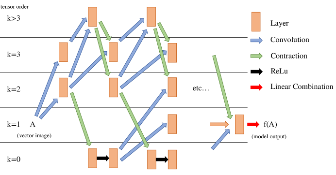
Figure 6: One possible architecture for a GI-Net that maps a vector image to a vector image when using convolution filters with tensor order $k^{\prime}\in\quantity{1,2}$, parity $p^{\prime}=+1$, max order $k=3$, and ReLu nonlinearities. Each layer is a block of multiple images that share tensor order. The blue arrows represent convolutions and raise the tensor order by 1 or 2. Contractions are applied when the tensor order goes above 3 to bring it down to 2 or 3, and when contracting to $k=0$ in order to apply the ReLu. This process continues until the final step where the only layer is order $k=1$, which is then combined using a parameterized linear combination.

5.2 Architecture Efficiency

Without specialized knowledge of what $B_{d}$-invariant convolution filters are relevant for our problem, we want to use all the filters at a specified tensor order in our convolution layers. Thus we can improve the efficiency of the GI-Net by eliminating any redundant filters. The first result follows from Proposition 2 and says that we may omit the ${k^{\prime}}_{(p^{\prime})}$-tensor filters if we are using the ${(k^{\prime}+2)}_{(p^{\prime})}$-tensor filters followed by taking all contractions.

Proposition 4.

Let $\mathcal{F}$ be the set of functions $f:\mathcal{A}_{N,d,k,p}\to\mathcal{A}_{N,d,k^{\prime\prime},p^{\prime\prime}}$ where each $f$ is a convolution with a $B_{d}$-invariant ${k^{\prime}}_{(p^{\prime})}$-tensor filter. Let $\mathcal{G}$ be the set of functions $g:\mathcal{A}_{N,d,k,p}\to\mathcal{A}_{N,d,k^{\prime\prime},p^{\prime\prime}}$ where each $g$ is a convolution with a $B_{d}$-invariant ${(k^{\prime}+2)}_{(p^{\prime})}$-tensor filter followed by a contraction. Then $\mathcal{F}\subseteq\mathcal{G}$.

See Appendix A for the proof. This proposition can be repeatedly applied so that if we conclude a GI-Net by taking all unique contractions, then we need only include filters of tensor order $k^{\prime}$ and $k^{\prime}-1$ to include all smaller tensor orders as well. The next result says that if the input and output parities of our network are equal, we may omit the ${k^{\prime}}_{(-)}$-tensor filters if we are using the ${(k^{\prime}+d)}_{(+)}$-tensor filters followed by taking all contractions.

Proposition 5.

Let $\mathcal{F}$ be the set of functions that preserve parity $f:\mathcal{A}_{N,d,k,p}\to\mathcal{A}_{N,d,k^{\prime\prime},p}$ where each $f$ is a convolution with a negative-parity ${k^{\prime}}_{(-)}$-tensor filter followed by a Levi-Civita contraction. Let $\mathcal{G}$ be the set of functions that preserve parity $g:\mathcal{A}_{N,d,k,p}\to\mathcal{A}_{N,d,k^{\prime\prime},p}$ where each $g$ is a convolution with a positive-parity ${(k^{\prime}+d)}_{(+)}$-tensor followed by $d-1$ contractions. Then $\mathcal{F}\subseteq\mathcal{G}$.

See Appendix A for the proof. We will employ these results in our numerical experiments to dramatically reduce the number of filters required.

Section 6 Numerical Experiments

Code to reproduce these experiments and build your own GI-Net is available at https://github.com/WilsonGregory/GeometricConvolutions. The code is built in Python using JAX.

The most natural problems for this model are those that we expect to obey the symmetries of the group $G_{N,d}$. We present two problems from physics that despite their simplicity, exhibit the powerful generalization properties of the equivariant model even in cases where we have few training points.

First, suppose we have as input a scalar image of point masses, and we want to learn the gravitational vector field induced by these masses. For this problem, we will work in two dimensions with image sidelength of 16, and the point charges are placed only at pixel centers, so the GI-Net is learning a function $f:\mathcal{A}_{16,2,0,+}\to\mathcal{A}_{16,2,1,+}$. To generate the data, we sampled the pixel locations uniformly without replacement 5 times to be point masses, and then we set their masses to be a uniform value between 0 and 1.

For a second problem, we consider several point charges in a viscous fluid. All the point charges have charge $+1$, so they repel each other. The position of the charges in the fluid would be described by an ordinary differential equation, and we can approximate that using Euler’s method:

$$x_{i}(t+\Delta t)=x_{i}(t)+\Delta t\,V(x_{i},t)~{},$$ (31)

where $x_{i}$ is a point, $\Delta t$ is one time step, and $V(x_{i},t)$ is the vector field at time $t$ induced by all particles other than $x_{i}$. We iterate this system some number of steps $T$, and the learning problem is the following: Given the initial charge field, can we predict the charge field after step $T$? For this toy problem we will again use an image in two dimensions of sidelength 16, so the function we are trying to learn is $f:\mathcal{A}_{16,2,1,+}\to\mathcal{A}_{16,2,1,+}$.

We took several precautions to make the data well behaved. Since the particles move freely in $\mathbb{R}^{2}$ but we learn on a discrete vector field grid, the vectors act erratic when the charge passes very closely to the center of the pixel. Thus we applied a sigmoid transform on the charge field vectors on the input and output:

$$Q(\vec{v},s)=\quantity(\frac{1}{1+e^{-\frac{\|\vec{v}\|}{s}}}-\frac{1}{2})\quantity(\frac{\vec{v}}{\|\vec{v}\|})~{},$$

where $\|\cdot\|$ is the usual Euclidean norm and $s$ is a parameter that we set to $0.2$. That is, the vector field is a nonlinear vector function of the original vector electric field. One advantage of learning on the charge field rather than the particles themselves is that vector field is discrete, but the vectors reflect the exact particle locations. However, if two particles start very close, it will appear that there is only a single particle on the charge vector field. To alleviate this problem, we iterated one step of Euler’s method, and treated that as the input to the neural network. Additionally, we initialized points within the central $8\times 8$ grid rather than the full $16\times 16$ grid so that the charges would be unlikely to leave the bounds of the grid by step $T$. See Figure 7 for example inputs and outputs for the two problems.

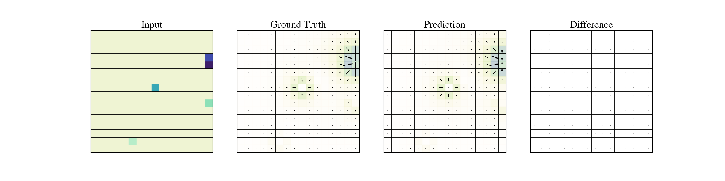
(a) (b)

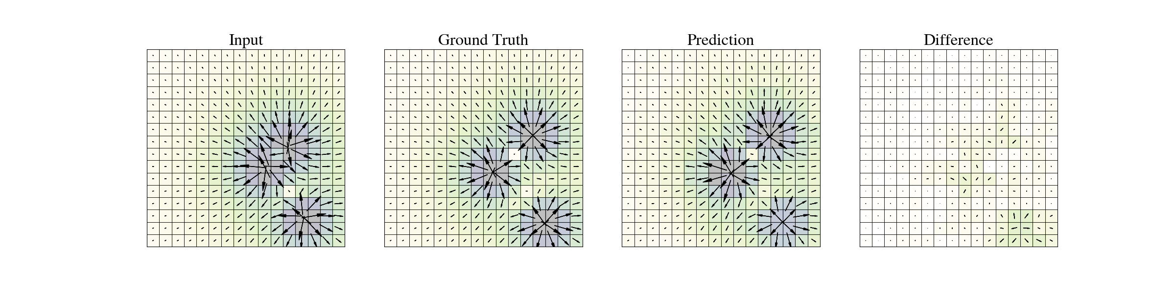
Figure 7: One test point each for the (a) gravitational field problem and the (b) moving point charge problem. The first two columns show the input and output to the problems respectively. The third column shows the model predicted output, and the fourth column shows the difference between the ground truth and the predicted output. To put the numerical results in context, the loss for the top row is 0.0177, while the loss for the bottom row is 2.061.

6.1 Architectures

For the gravity problem, the architecture that we choose has 3 convolution layers followed by all contractions that reduce to $k=1$, and then a parameterized linear combination of the resulting images. The second convolution layer uses dilations that range from 1 to 15, and the third convolution layer uses dilations from 1 to 7. For our loss we use the root mean squared error (RMSE). The baseline architecture is built to have similar structure with 3 convolution layers with the same dilations, but also have a number parameters on the same order of magnitude. We treat the dilations as creating a separate channel. The sequence of channel depth is the following:

$$1\to 2\to(15*2)\to(7*2)\to 2$$

To get from the output of the 3rd convolution which is 2 filters across 7 dilations, we take a parameterized sum across the dilations to get an image with 2 channels, which is the number of channels we need for a vector image. See Table 2 for additional info about the filters and number of parameters.

problem	model	$M$	$k^{\prime}$	$p^{\prime}$	# layers	depths	# params
gravity	GI-Net	3	0,1	$+1$	3	1	3 085
	baseline	3	0		3	2,$15*2,7*2$	4 345
charge	GI-Net	3	1,2	$+1$	9	1	22 986
	baseline	3	0		9	20,…,20,2	25 920

Table 2: Comparison of the different model architectures used for the two problems. The values of $M,k^{\prime},p^{\prime}$ represent the sidelength, tensor order, and parity of the convolutional filters. The baseline models do not have a parity because those filters are learned rather than fixed ahead of time.

The moving charges problem is more difficult, so we choose a more complex architecture. We have 9 convolution layers, with dilations of $1,2,4,2,1,1,2,1,1$ in that order. Each convolution is followed by a nonlinear activation layer with a Leaky ReLu with negative slope of 0.01. This non-linearity seemed to perform best among the ones we tried. We then finish with the usual contraction layer and linear combination, and our loss is again the RMSE. For the baseline model, we use identical number of convolution layers, dilations, nonlinearities, and loss. The only difference is that we only use scalar filters, so we increase the depth of each layer to 20 except for the final output layer which must have a depth of 2 because we are learning a vector image.

6.2 Training

For all models, we trained the network using stochastic gradient descent with the Adam optimizer and an exponential learning rate decay that started at 0.005, has transition steps equal to the number of batches per epoch, and has a decay of 0.995. The one exception was the baseline model for the moving charges problem where we started with a learning rate of 0.001. These values were found with a limited grid search. For both problems and both models we initialized the parameters as Gaussian noise with mean 0 and standard deviation 0.1.

For the gravitational field problem, we created a test set of 10 images, a validation set of 5 images, and training sets ranging in size from 5 to 50 images. For the moving charges problem we created a test set of 10 images, a validation set of 10 images, and training sets ranging in size from 5 to 100 images. We used training batch sizes equal to $0.2$ the training set size. For all models we trained them until the error on the validation set had not improved in 20 epochs.

6.3 Results

Given sufficient data, both the GI-Net and the baseline model are able to perform well on the test data set. The RMSE carries very little information without further context, but we can see from the examples in Figure 7 that low error corresponds to only small differences between the ground truth output and the predicted output. By comparing the GI-Net to our simple CNN baseline we can see the advantages of the equivariant model.

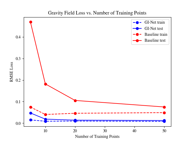
(a) Gravitational Field Loss
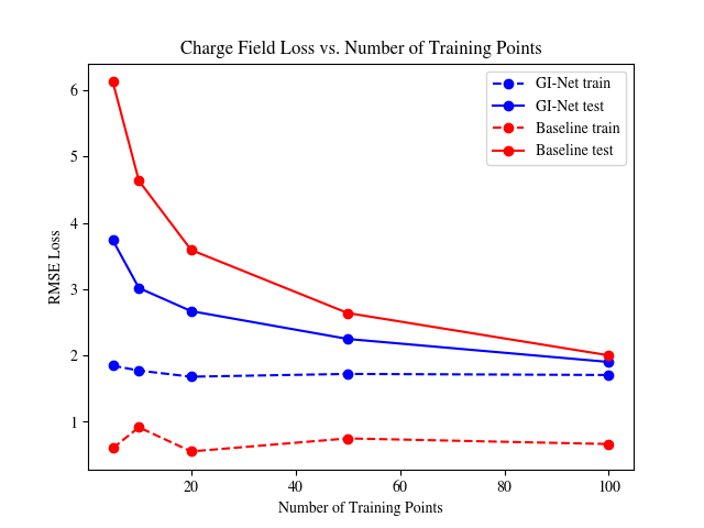
(b) Charge Field Loss

Figure 8: Comparison between baseline model and GI-Net as a function of the number of points in the training data set. The GI-Net have smaller testing loss when the training data set is small, even when the baseline model achieves better training error in the case of the moving charges problem.

In Figure 8(a), with only 10 data points, the test error of the GI-Net is almost equal to the training error, suggesting that the model is able to generalize well from just a few small examples. By contrast, the baseline model requires at least 50 training points to get its test error as close to its training error. Additionally, even when the baseline model has enough points, its error is still higher overall compared to the GI-Net.

Likewise, in Figure 8(b) the gap between the test error and training error for the baseline model is much larger than the same gap for the GI-Net. In this case, the GI-Net and the baseline model reach the same test error when training off 100 points, despite the baseline model having smaller training error. This again suggests that the GI-Net does a better job generalizing, especially when the training data set is small.

Section 7 Related work

Restricting machine learning models to use functions that are equivariant to some group action is a powerful idea that has the potential to improve generalization and reduce training requirements. When we expect our target function to be equivariant to that group, this restriction improves the model’s generalization and accuracy (see for instance [16, 15, 47]) and is a powerful remedy for data scarcity (see [49]). Equivariant networks, in certain cases, can approximate any continuous equivariant function (see [53, 13, 3, 31]).

There is a wide variety of strategies to design equivariant maps (e.g. [7, 48]). One class of methods, employed in this work, is group convolution, either on the group or on the homogeneous space where the features lie. Our generalization of convolution replaces arbitrary products with the outer product of tensors. Our approach is related to [4], which employs a Clifford Algebra.

Other strategies to design equivariant maps use irreducible representations or invariant theory to parameterize the space of equivariant functions. The first work using representation theory for invariant and equivariant neural networks was the paper of Wood et al. [50] from 1996. More recent incarnations of these ideas include [36, 8, 7, 6, 10, 17]. One can use classical invariant theory to compute the generators of the algebra of invariant polynomials. For instance, in [2] we show how to use the generators of the algebra of invariant polynomials to produce a parameterization of equivariant functions for certain groups and actions. This approach is inspired by the physical sciences, where the data is subject to rules coming from coordinate freedoms and conservation laws. In previous work [44, 45, 52] we used these geometric rules to develop modified machine-learning methods that are restricted to exactly obey group-theoretic equivariances in physics contexts. Similar ideas have been explored in [23, 20].

See appendix B for a more in depth description of the mathematical details of the related work.

Section 8 Discussion

This paper presents a flexible new model, the GeometricImageNet, which parameterizes functions that map geometric images to geometric images. It capitalizes on the vector or tensor structure of the image contents. The flexibility, coupled with the easy restriction to $G_{N,d}$-equivariant functions, makes the model ideal for tackling many problems from the natural sciences in a principled way.

The added flexibility of tensors comes with a cost. Taking repeated convolutions with tensor filters grows the the tensor order and thus, with naive representations, the memory requirements of the network. We see the consequences of this issue when trying to numerically demonstrate that we have characterized all the equivariant homogeneous polynomials (Section 4). We also encounter this issue when solving problems in Section 6; fortunately, it appears that capping the maximum tensor order limits the memory requirements without much associated loss in performance.

Another shortcoming of this work is that we work with discrete symmetries rather than continuous symmetries. We expect invariance and equivariance with respect to rotations other than 90 degrees to appear in nature, but the images that we work with are always going to be $d$-cube lattices of points. Thus we use the group $G_{N,d}$ to avoid interpolating rotated images and working with approximate equivariances. This simplifies the mathematical results, and we see empirically that we still have the benefits of rotational equivariance. However, there are other possible image representations that might create more continuous concepts of images. For example, if the data is on the surface of a sphere, it could be represented with tensor spherical harmonics, and be subject to transformations by a continuous rotation group.

There are many possible future directions that could be explored. It is an open question to understand the full expressive power of the model outside the few cases we were able to test in Section 4. Additionally, there are likely improvements to be made to both the time and space efficiency of the GeometricImageNet. Finally, there are many exciting applications in fluid dynamics, astronomy, climate science, biology, and others that could benefit from this physics-informed machine learning approach.

Acknowlegements:

It is a pleasure to thank Roger Blandford (Stanford), Drummond Fielding (Flatiron), Leslie Greengard (Flatiron), Ningyuan (Teresa) Huang (JHU), Kate Storey-Fisher (NYU), and the Astronomical Data Group at the Flatiron Institute for valuable discussions and input. This project made use of Python 3 [42], numpy [24], matplotlib [28], and cmastro [38]. All the code used for making the data and figures in this paper is available at https://github.com/WilsonGregory/GeometricConvolutions.

Funding:

WG was supported by an Amazon AI2AI Faculty Research Award. BBS was supported by ONR N00014-22-1-2126. MTA was supported by H2020-MSCA-RISE-2017, Project 777822, and from Grant PID2019-105599GB-I00, Ministerio de Ciencia, Innovación y Universidades, Spain. SV was partly supported by the NSF–Simons Research Collaboration on the Mathematical and Scientific Foundations of Deep Learning (MoDL) (NSF DMS 2031985), NSF CISE 2212457, ONR N00014-22-1-2126 and an Amazon AI2AI Faculty Research Award.

Appendix A Propositions and Proofs

This section provides propositions and their proofs that are necessary for some of the results earlier in the paper. In many of these proofs we will show that the property holds for some arbitrary pixel index $\bar{\imath}$, so it must hold for all pixels. First we state two well known results from tensor analysis.

Proposition 6.

The Kronecker delta, Definition 4, is invariant to the group $B_{d}$.

Proof.

Let $g\in B_{d}$ with matrix representation $M(g)$. The Kronecker delta $\delta$ is a ${2}_{(+)}$-tensor so the action of $g$ is by conjugation. Thus,

$$g\cdot\delta=M(g)\delta M(g)^{T}=M(g)M(g)^{T}=\delta$$

since the Kronecker delta is also the $d\times d$ identity matrix and the matrix representations of $B_{d}$ are orthogonal. ∎

Proposition 7.

The Levi-Civita symbol, Definition 5, is invariant to the group $B_{d}$.

Proof.

The Levi-Civita tensor $\epsilon\in(\mathbb{R}^{d})^{\otimes d}$ is defined so as to satisfy the identity

$$\epsilon^{\sigma}=\operatorname{sgn}(\sigma)\epsilon,$$

where $\sigma\in S_{d}$ is a permutation of the indices (cf. Definition 7). Thus it is an alternating tensor of order $d$. It is well-known (e.g., [21, p. 160] or [35, p. 13]) that the subspace of these is (one-dimensional and) stable under the action of $GL(\mathbb{R}^{d})$ on $(\mathbb{R}^{d})^{\otimes d}$ given by linear extension of $M\cdot(u_{1}\otimes\dots\otimes u_{d}):=(Mu_{1})\otimes\dots\otimes(Mu_{d})$, where $M\in GL(\mathbb{R}^{d})$ is an arbitrary invertible matrix, and that $M$ acts on this subspace by multiplication by $\det(M)$. Thus

$$M\cdot\epsilon=\det(M)\epsilon,$$

where the action on the left is the one just described. Using instead the action under consideration throughout this paper, i.e., the action of $O(d)\subset GL(\mathbb{R}^{d})$ defined by equation (1) and Definition 1, we get an additional determinant factor on the right side because $\epsilon$ is a ${d}_{(-)}$-tensor. In other words, $g\cdot\epsilon=\det(M(g))^{2}\epsilon$. Since $\det(M(g))^{2}=1$ for all $g\in O(d)$, we conclude that $g\cdot\epsilon=\epsilon$. ∎

Next we state several properties of geometric convolution that are well known for the general mathematical definition of convolution.

Properties (Convolution).

Given $A,B\in\mathcal{A}_{N,d,k,p},C,S\in\mathcal{A}_{M,d,k^{\prime},p^{\prime}},\tau\in(\mathbb{Z}/N\mathbb{Z})^{d}$ and $\alpha,\beta\in\mathbb{R}$, then the following properties hold:

1. The convolution operation is translation equivariant:

   $$(L_{\tau}A)*C=L_{\tau}(A*C)$$ (32)

2. The convolution operation is linear in the geoemetric image:

   $$(\alpha A+\beta B)*C=\alpha(A*C)+\beta(B*C)$$ (33)

   It is also linear in the filters:

   $$A*(\alpha C+\beta S)=\alpha(A*C)+\beta(A*S)$$ (34)

Proof.

First we will prove (32). Let $A,C$, and $\tau$ be as above and let $\bar{\imath}$ be a pixel index of $L_{\tau}A*C$. Then:

$$(L_{\tau}A\ast C)(\bar{\imath}) =\sum_{\bar{a}\in[-m,m]^{d}}(L_{\tau}A)(\bar{\imath}-\bar{a})\otimes C(\bar{a}+\bar{m})$$

$$=\sum_{\bar{a}\in[-m,m]^{d}}A(\bar{\imath}-\bar{a}-\tau)\otimes C(\bar{a}+\bar{m})$$

$$=\sum_{\bar{a}\in[-m,m]^{d}}A((\bar{\imath}-\tau)-\bar{a})\otimes C(\bar{a}+\bar{m})$$

$$=(A\ast C)(\bar{\imath}-\tau)$$

$$=L_{\tau}(A\ast C)(\bar{\imath})$$

Now we will prove (33). Let $A,B,C,\alpha,$ and $\beta$ be as above and let $\bar{\imath}$ be a pixel index of $(\alpha A+\beta B)*C$. Then:

$$((\alpha A+\beta B)*C)(\bar{\imath}) =\sum_{\bar{a}\in[-m,m]^{d}}(\alpha A+\beta B)(\bar{\imath}-\bar{a})\otimes C(\bar{a}+\bar{m})$$

$$=\sum_{\bar{a}\in[-m,m]^{d}}(\alpha A(\bar{\imath}-\bar{a})+\beta B(\bar{\imath}-\bar{a}))\otimes C(\bar{a}+\bar{m})$$

$$=\sum_{\bar{a}\in[-m,m]^{d}}\alpha A(\bar{\imath}-\bar{a})\otimes C(\bar{a}+\bar{m})+\beta B(\bar{\imath}-\bar{a})\otimes C(\bar{a}+\bar{m})$$

$$=\alpha\sum_{\bar{a}\in[-m,m]^{d}}A(\bar{\imath}-\bar{a})\otimes C(\bar{a}+\bar{m})+\beta\sum_{\bar{a}\in[-m,m]^{d}}B(\bar{\imath}-\bar{a})\otimes C(\bar{a}+\bar{m})$$

$$=\alpha(A*C)(\bar{\imath})+\beta(B*C)(\bar{\imath})$$

Now we will prove (34). Let $A,C,S,\alpha,$ and $\beta$ be as above and let $\bar{\imath}$ be a pixel index. Then:

$$\quantity(A*(\alpha C+\beta S))(\bar{\imath}) =\sum_{\bar{a}\in[-m,m]^{d}}A(\bar{\imath}-\bar{a})\otimes(\alpha C+\beta S)(\bar{a}+\bar{m})$$

$$=\sum_{\bar{a}\in[-m,m]^{d}}A(\bar{\imath}-\bar{a})\otimes\alpha C(\bar{a}+\bar{m})+A(\bar{\imath}-\bar{a})\otimes\beta S(\bar{a}+\bar{m})$$

$$=\alpha\sum_{\bar{a}\in[-m,m]^{d}}A(\bar{\imath}-\bar{a})\otimes C(\bar{a}+\bar{m})+\beta\sum_{\bar{a}\in[-m,m]^{d}}A(\bar{\imath}-\bar{a})\otimes S(\bar{a}+\bar{m})$$

$$=\alpha(A*C)(\bar{\imath})+\beta(A*S)(\bar{\imath})$$

Thus we have our result. ∎

Now we will state several properties of the contraction.

Properties (Contraction).

Given $A,B\in\mathcal{A}_{N,d,k,p},S\in\mathcal{A}_{N,d,k^{\prime},p^{\prime}},C\in\mathcal{C}_{M,d,k^{\prime},p^{\prime}}$, $g\in G_{N,d},\mu,\nu,\rho,\sigma\in[k]$ all distinct, and $\alpha,\beta\in\mathbb{R}$, then the following properties hold:

1. Contraction indices can be swapped:

   $$T(A,\mu,\nu)=T(A,\nu,\mu)$$ (35)

2. Contractions on distinct indices commute:

   $$T_{M}(A,(\mu,\nu),(\rho,\sigma))=T_{M}(A,(\rho,\sigma),(\mu,\nu))$$ (36)

3. Contractions are equivariant to $G_{N,d}$:

   $$g\cdot T(A,\mu,\nu)=T(g\cdot A,\mu,\nu)$$ (37)

4. Contractions are linear functions:

   $$T(\alpha A+\beta B,\mu,\nu)=\alpha\,T(A,\mu,\nu)+\beta\,T(B,\mu,\nu)$$ (38)

5. Contractions commute with the outer product. If $\mu,\nu\in[k],\mu\not=\nu$ then:

   $$T(A\otimes S,\mu,\nu)=T(A,\mu,\nu)\otimes S$$ (39)

   Otherwise, if $\mu,\nu\in\quantity{k+1,\ldots,k+k^{\prime}},\mu\not=\nu$ then:

   $$T(A\otimes S,\mu,\nu)=A\otimes T(S,\mu-k,\nu-k)$$ (40)

6. Contractions commute with convolutions. If $\mu,\nu\in[k]$ distinct then:

   $$T(A*C,\mu,\nu)=T(A,\mu,\nu)*C$$ (41)

   Otherwise, if $\mu,\nu\in\quantity{k+1,\ldots,k+k^{\prime}}$ distinct then:

   $$T(A*C,\mu,\nu)=A*T(C,\mu-k,\nu-k)$$ (42)

Proof.

Equation (35) follows directly from the definition, 6. Now we will prove (36). Let $A,\mu,\nu,\rho,$ and $\sigma$ be defined as above, let $\bar{\imath}$ be a pixel index of $A$, and let $a\in\mathcal{T}_{d,k,p}$ be the tensor at that index. Since contractions are applied the same to all pixels, it suffices to show that this proposition is true for this pixel. The result then follows quickly from the definition:

$$\quantity[T_{M}(a,(\mu,\nu),(\rho,\sigma))]_{\quantity{i_{1},\ldots,i_{k}}\setminus\quantity{i_{\mu},i_{\nu},i_{\rho},i_{\sigma}}} =[\delta]_{i_{\rho},i_{\sigma}}\quantity([\delta]_{i_{\mu},i_{\nu}}[a]_{i_{1},\ldots,i_{k}})$$

$$=[\delta]_{i_{\mu},i_{\nu}}[\delta]_{i_{\rho},i_{\sigma}}[a]_{i_{1},\ldots,i_{k}}$$

$$=[\delta]_{i_{\mu},i_{\nu}}\quantity([\delta]_{i_{\rho},i_{\sigma}}[a]_{i_{1},\ldots,i_{k}})$$

$$=\quantity[T_{M}(a,(\rho,\sigma),(\mu,\nu))]_{\quantity{i_{1},\ldots,i_{k}}\setminus\quantity{i_{\mu},i_{\nu},i_{\rho},i_{\sigma}}}$$

Next we will prove (37). Let $A,\mu,$ and $\nu$ be defined as above and let $\bar{\imath}$ be a pixel of $A$. First we will show that contractions are equivariant to translations. Let $\tau\in(\mathbb{Z}/N\mathbb{Z})^{d}$. Then

$$T(L_{\tau}A,\mu,\nu)(\bar{\imath}) =T((L_{\tau}A)(\bar{\imath}),\mu,\nu)$$

$$=T(A(\bar{\imath}-\tau),\mu,\nu)$$

$$=T(A,\mu,\nu)(\bar{\imath}-\tau)$$

$$=(L_{\tau}T(A,\mu,\nu))(\bar{\imath})$$

Thus contractions are equivariant to translations. Now we will show that contractions are equivariant to $B_{d}$. Let $g\in B_{d}$, and denote $A(g^{-1}\bar{\imath})=a$. Then by equation (4) we have:

$$T(g\cdot A,\mu,\nu)(\bar{\imath}) =T((g\cdot A)(\bar{\imath}),\mu,\nu)$$

$$=T\quantity(g\cdot A(g^{-1}\cdot\bar{\imath}),\mu,\nu)$$

$$=T\quantity(g\cdot a,\mu,\nu)$$

$$=[\delta]_{i_{\mu},i_{\nu}}[g\cdot a]_{i_{1},\ldots,i_{\mu},\ldots,i_{\nu},\ldots i_{k}}$$

$$=[\delta]_{i_{\mu},i_{\nu}}[a]_{j_{1},\ldots,j_{k}}\prod_{q\in[k]}[M(g)]_{i_{q},j_{q}}$$

$$=[\delta]_{i_{\mu},i_{\nu}}[a]_{j_{1},\ldots,j_{k}}[M(g)]_{i_{\mu},j_{\mu}}[M(g)]_{i_{\nu},j_{\nu}}\prod_{q\in[k]\setminus\quantity{\mu,\nu}}[M(g)]_{i_{q},j_{q}}$$

$$=\quantity([\delta]_{i_{\mu},i_{\nu}}[M(g)]_{i_{\mu},j_{\mu}}[M(g)]_{i_{\nu},j_{\nu}})[a]_{j_{1},\ldots,j_{k}}\prod_{q\in[k]\setminus\quantity{\mu,\nu}}[M(g)]_{i_{q},j_{q}}$$

$$=[\delta]_{j_{\mu},j_{\nu}}[a]_{j_{1},\ldots,j_{k}}\prod_{q\in[k]\setminus\quantity{\mu,\nu}}[M(g)]_{i_{q},j_{q}}$$

Note that $\quantity([\delta]_{i_{\mu},i_{\nu}}[M(g)]_{i_{\mu},j_{\mu}}[M(g)]_{i_{\nu},j_{\nu}})$ is the action of $g$ on $\delta$. Thus it equals $[\delta]_{j_{\mu}j_{\nu}}$ by Proposition 6, as shown in the last step. Hence:

$$T(g\cdot A,\mu,\nu)(\bar{\imath}) =\quantity[T(a,\mu,\nu)]_{\quantity{j_{1},\ldots,j_{k}}\setminus\quantity{j_{\mu},j_{\nu}}}\prod_{q\in[k]\setminus\quantity{\mu,\nu}}[M(g)]_{i_{q},j_{q}}$$

$$=g\cdot T(A(g^{-1}\cdot\bar{\imath}),\mu,\nu)$$

$$=g\cdot T(A,\mu,\nu)(g^{-1}\cdot\bar{\imath})$$

$$=\quantity(g\cdot T(A,\mu,\nu))(\bar{\imath})$$

Therefore, since contractions are equivariant to the generators of $G_{N,d}$, it is equivariant to the group.

Next we will prove (38). Let $A,B,\mu,$ and $\nu$ be defined as above, let $\bar{\imath}$ be a pixel index of $(\alpha A+\beta B)$, and let $a,b\in\mathcal{T}_{d,k,p}$ be the tensors of $A$ and $B$ at that pixel index. Then:

$$T(\alpha A+\beta B,\mu,\nu)(\bar{\imath})_{\quantity{i_{1},\ldots,i_{k}}\setminus{i_{\mu},i_{\nu}}} =T(\alpha A(\bar{\imath})+\beta B(\bar{\imath}),\mu,\nu)_{\quantity{i_{1},\ldots,i_{k}}\setminus{i_{\mu},i_{\nu}}}$$

$$=T(\alpha a+\beta b,\mu,\nu)_{\quantity{i_{1},\ldots,i_{k}}\setminus{i_{\mu},i_{\nu}}}$$

$$=\delta_{i_{\mu},i_{\nu}}(\alpha a+\beta b)_{i_{1},\ldots,i_{k}}$$

$$=\delta_{i_{\mu},i_{\nu}}(\alpha a)_{i_{1},\ldots,i_{k}}+\delta_{i_{\mu},i_{\nu}}(\beta b)_{i_{1},\ldots,i_{k}}$$

$$=\alpha\quantity(\delta_{i_{\mu},i_{\nu}}a_{i_{1},\ldots,i_{k}})+\beta\quantity(\delta_{i_{\mu},i_{\nu}}b_{i_{1},\ldots,i_{k}})$$

$$=\alpha\cdot T(a,\mu,\nu)_{\quantity{i_{1},\ldots,i_{k}}\setminus{i_{\mu},i_{\nu}}}$$

$$\hskip 14.22636pt+\beta\cdot T(b,\mu,\nu)_{\quantity{i_{1},\ldots,i_{k}}\setminus{i_{\mu},i_{\nu}}}$$

$$=\alpha\cdot T(A,\mu,\nu)(\bar{\imath})_{\quantity{i_{1},\ldots,i_{k}}\setminus{i_{\mu},i_{\nu}}}$$

$$\hskip 14.22636pt+\beta\cdot T(B,\mu,\nu)(\bar{\imath})_{\quantity{i_{1},\ldots,i_{k}}\setminus{i_{\mu},i_{\nu}}}$$

Thus we have shown (38).

Now we will prove (39). Let $A,S$ be as described, let $\mu,\nu\in[k]$ distinct, let $\bar{\imath}$ be a pixel index of $A$ and $S$, and let $A(\bar{\imath})=a$ and $S(\bar{\imath})=s$ be the tensors at that pixel index. Then:

$$\quantity[T(A\otimes S,\mu,\nu)(\bar{\imath})]_{i_{1},\ldots,i_{k+k^{\prime}}\setminus\quantity{i_{\mu},i_{\nu}}} =\quantity[T(A(\bar{\imath})\otimes S(\bar{\imath}),\mu,\nu)]_{i_{1},\ldots,i_{k+k^{\prime}}\setminus\quantity{i_{\mu},i_{\nu}}}$$

$$=\quantity[T(a\otimes s,\mu,\nu)]_{i_{1},\ldots,i_{k+k^{\prime}}\setminus\quantity{i_{\mu},i_{\nu}}}$$

$$=[\delta]_{i_{\mu},i_{\nu}}[a\otimes s]_{i_{1},\ldots,i_{k+k^{\prime}}}$$

$$=[\delta]_{i_{\mu},i_{\nu}}[a]_{i_{1},\ldots i_{k}}[s]_{i_{k+1},\ldots,i_{k+k^{\prime}}}$$

$$=[T(a,\mu,\nu)]_{i_{1},\ldots,i_{k}\setminus\quantity{i_{\mu},i_{\nu}}}[s]_{i_{k+1},\ldots,i_{k+k^{\prime}}}$$

$$=[T(a,\mu,\nu)\otimes s]_{i_{1},\ldots,i_{k+k^{\prime}}\setminus\quantity{i_{\mu},i_{\nu}}}$$

$$=[(T(A,\mu,\nu)\otimes S)(\bar{\imath})]_{i_{1},\ldots,i_{k+k^{\prime}}\setminus\quantity{i_{\mu},i_{\nu}}}$$

This gives us (39). Now suppose instead, $\mu,\nu\in\quantity{k+1,\ldots,k+k^{\prime}}$. Skipping a few of the initial steps that are the same as above, we have:

$$\quantity[T(A\otimes S,\mu,\nu)(\bar{\imath})]_{i_{1},\ldots,i_{k+k^{\prime}}\setminus\quantity{i_{\mu},i_{\nu}}} =[\delta]_{i_{\mu},i_{\nu}}[a]_{i_{1},\ldots i_{k}}[s]_{i_{k+1},\ldots,i_{k+k^{\prime}}}$$

$$=[a]_{i_{1},\ldots i_{k}}[\delta]_{i_{\mu},i_{\nu}}[s]_{i_{k+1},\ldots,i_{k+k^{\prime}}}$$

$$=[a]_{i_{1},\ldots i_{k}}[T(s,\mu-k,\nu-k)]_{i_{k+1},\ldots,i_{k+k^{\prime}}\setminus\quantity{i_{\mu},i_{\nu}}}$$

$$=[a\otimes T(s,\mu-k,\nu-k)]_{i_{1},\ldots,i_{k+k^{\prime}}\setminus\quantity{i_{\mu},i_{\nu}}}$$

$$=[\quantity(A\otimes T(S,\mu-k,\nu-k))(\bar{\imath})]_{i_{1},\ldots,i_{k+k^{\prime}}\setminus\quantity{i_{\mu},i_{\nu}}}$$

Thus we have our result.

The properties (41) and (42) follow from (39) and (40). Let $A,C$ be as described above, let $\mu,\nu\in[k]$ distinct, and let $\bar{\imath}$ be a pixel index of $A*C$. Then by the previous results and the linearity of contraction we have:

$$T(A*C,\mu,\nu)(\bar{\imath}) =T((A*C)(\bar{\imath}),\mu,\nu)$$

$$=T\quantity(\sum_{\bar{a}\in[-m,m]^{d}}A(\bar{\imath}-\bar{a})\otimes C(\bar{a}+\bar{m}),\mu,\nu)$$

$$=\sum_{\bar{a}\in[-m,m]^{d}}T\quantity(A(\bar{\imath}-\bar{a})\otimes C(\bar{a}+\bar{m}),\mu,\nu)$$

$$=\sum_{\bar{a}\in[-m,m]^{d}}T(A(\bar{\imath}-\bar{a}),\mu,\nu)\otimes C(\bar{a}+\bar{m})$$

$$=T(A,\mu,\nu)*C$$

Likewise, if $\mu,\nu\in\quantity{k+1,\ldots,k+k^{\prime}}$ distinct then:

$$T(A*C,\mu,\nu)(\bar{\imath}) =\sum_{\bar{a}\in[-m,m]^{d}}T\quantity(A(\bar{\imath}-\bar{a})\otimes C(\bar{a}+\bar{m}),\mu,\nu)$$

$$=\sum_{\bar{a}\in[-m,m]^{d}}A(\bar{\imath}-\bar{a})\otimes T(C(\bar{a}+\bar{m}),\mu-k,\nu-k)$$

$$=A*T(C,\mu-k,\nu-k)$$

Thus we have our result. ∎

Next we will state one property of the Levi-Civita contraction, but many properties of regular contractions follow for Levi-Civita Contractions.

Properties (Levi-Civita Contraction).

Let $A\in\mathcal{A}_{N,d,k,p}$ for $k\geq d-1,C\in\mathcal{A}_{M,d,k^{\prime},p^{\prime}}$, and $\mu_{1},\ldots,\mu_{d-1}\in[k]$ distinct. Then the following properties hold:

1. Levi-Civita Contractions are equivariant to $G_{N,d}$:

   $$g\cdot T_{LC}(A,\mu_{1},\ldots,\mu_{d-1})=T_{LC}(g\cdot A,\mu_{1},\ldots,\mu_{d-1})$$ (43)

Proof.

W will prove (43) using the equivariance of the contraction (37). Let $A$ and $\mu_{1},\ldots,\mu_{\ell}$ be as described and let $\bar{\imath}$ be a pixel index. Then

$$\quantity(g\cdot T_{LC}(A,\mu_{1},\ldots,\mu_{d-1}))(\bar{\imath}) =g\cdot\quantity(T_{LC}(A,\mu_{1},\ldots,\mu_{d-1})(g^{-1}\cdot\bar{\imath}))$$

$$=g\cdot\quantity(T_{LC}(A(g^{-1}\cdot\bar{\imath}),\mu_{1},\ldots,\mu_{d-1}))$$

$$=g\cdot T_{M}\quantity(A\quantity(g^{-1}\cdot\bar{\imath})\otimes\epsilon,(\mu_{1},k^{\prime}+1),\ldots,(\mu_{d-1},k^{\prime}+d-1))$$

$$=T_{M}\quantity(g\cdot\quantity(A\quantity(g^{-1}\cdot\bar{\imath})\otimes\epsilon),(\mu_{1},k^{\prime}+1),\ldots,(\mu_{d-1},k^{\prime}+d-1))$$

$$=T_{M}\quantity(g\cdot A\quantity(g^{-1}\cdot\bar{\imath})\otimes g\cdot\epsilon,(\mu_{1},k^{\prime}+1),\ldots,(\mu_{d-1},k^{\prime}+d-1))$$

$$=T_{M}\quantity((g\cdot A)(\bar{\imath})\otimes\epsilon,(\mu_{1},k^{\prime}+1),\ldots,(\mu_{d-1},k^{\prime}+d-1))$$

$$=T_{LC}(g\cdot A,\mu_{1},\ldots,\mu_{d-1})(\bar{\imath})$$

This proof relies on the fact that $g\cdot\epsilon=\epsilon$ given by Proposition 7. Thus we have our result. ∎

Before proving Proposition 1, we must prove a short lemma about performing a convolution with a filter of size $N+1$ on an image of size $N$.

Lemma 2.

Given $A\in\mathcal{A}_{N,d,k,p}$ a geometric image and $C\in\mathcal{A}_{N+1,d,k^{\prime},p^{\prime}}$ a geometric filter where $M=N+1$, there exists $C^{\prime}\in\mathcal{A}_{N+1,d,k^{\prime},p^{\prime}}$ such that $A*C^{\prime}=A*C$ and $C^{\prime}(\bar{\imath})$ is the zero ${k^{\prime}}_{(p^{\prime})}$-tensor, for $\bar{\imath}\in[0,N]^{d}\setminus[0,N-1]^{d}$. That is, $C^{\prime}$ is totally defined by $N^{d}$ pixels, and every pixel with an $N$ in the index is equal to the zero ${k^{\prime}}_{(p^{\prime})}$-tensor.

Proof.

Let $A$ and $C$ be defined as above. Thus

$$M=N+1\Rightarrow 2m+1=N+1\Rightarrow 2m=N$$

Consider the convolution definition (11) where we have $A(\bar{\imath}-\bar{a})$ where $\bar{\imath}\in[0,N-1]^{d}$ and $\bar{a}\in[-m,m]^{d}$. Since $A$ is on the $d$-torus, then whenever the $\ell^{th}$ index of $\bar{a}=-m$ we have:

$$\quantity(\bar{\imath}_{\ell}-\bar{a}_{\ell})\mod N =\quantity(\bar{\imath}_{\ell}-(-m))\mod N$$

$$=\quantity(\bar{\imath}_{\ell}+m)\mod 2m$$

$$=\quantity(\bar{\imath}_{\ell}+m-2m)\mod 2m$$

$$=\quantity(\bar{\imath}_{\ell}-m)\mod N$$

Thus, any time there is an index $\bar{a}$ with a value $\pm m$, we have an equivalence class under the torus with all other indices with flipped sign of the $m$ in any combination. If $\quantity{\bar{a}}$ is this equivalence class, we may group these terms in the convolution sum:

$$\sum_{\bar{a}^{\prime}\in\quantity{\bar{a}}}A(\bar{\imath}-\bar{a}^{\prime})\otimes C(\bar{a}^{\prime}+\bar{m})=\sum_{\bar{a}^{\prime}\in\quantity{\bar{a}}}A(\bar{\imath}-\bar{a})\otimes C(\bar{a}^{\prime}+\bar{m})=A(\bar{\imath}-\bar{a})\otimes\quantity(\sum_{\bar{a}^{\prime}\in\quantity{\bar{a}}}C(\bar{a}^{\prime}+\bar{m}))$$

Thus, we may pick a single pixel of the convolutional filter $C$, set it equal to $\sum_{\bar{a}^{\prime}\in\quantity{\bar{a}}}C(\bar{a}^{\prime}+\bar{m})$, and set all other pixels of the equivalence class to the zero ${k^{\prime}}_{(p^{\prime})}$-tensor without changing the convolution. We choose the nonzero pixel to be the one whose index has all $-m$ instead of $m$. Thus we can define the filter $C$ by $N^{d}$ pixels rather than $(N+1)^{d}$ pixels, and we have our result. ∎

Proof of Proposition 1:

Proposition.

A function $f:\mathcal{A}_{N,d,k,p}\to\mathcal{A}_{N,d,k+k^{\prime},p\,p^{\prime}}$ is a translation equivariant linear function if and only if it is the convolution with a geometric filter $C\in\mathcal{A}_{M,d,2k+k^{\prime},p^{\prime}}$ followed by $k$ contractions. When $N$ is odd, $M=N$, otherwise $M=N+1$.

Proof.

Let $\mathcal{F}=\quantity{f:\mathcal{A}_{N,d,k,p}\to\mathcal{A}_{N,d,k+k^{\prime},p\,p^{\prime}}}$ where each function $f$ is linear and equivariant to translations. Let $\mathcal{G}=\quantity{g:\mathcal{A}_{N,d,k,p}\to\mathcal{A}_{N,d,k+k^{\prime},p\,p^{\prime}}}$ where each $g$ is defined as $g(A)=T_{M}(A*C,(1,k+1),\ldots,(k,2k))$ for some $C\in\mathcal{A}_{M,d,2k+k^{\prime},p^{\prime}}$. If $N$ is odd then $M=N$, otherwise $M=N+1$. It suffices to show that $\mathcal{F}=\mathcal{G}$.

First we will show that $\mathcal{G}\subseteq\mathcal{F}$. Let $g\in\mathcal{G}$. By properties (33) and (38) both convolutions and contractions are linear. Additionally, by properties (32) and (37) convolutions and contractions are both equivariant to translations. Thus $g\in\mathcal{F}$, so $\mathcal{G}\subseteq\mathcal{F}$.

Now we will show that $\dim(\mathcal{F})=\dim(\mathcal{G})$. Let $f\in\mathcal{F}$. By Definition 1, $T_{d,k,p}\cong\quantity(\mathbb{R}^{d})^{\otimes k}$ equipped with the group action of $O(d)$. Then by Definition 8, $\mathcal{A}_{N,d,k,p}$ is the space of functions $A:[N]^{d}\to\mathcal{T}_{d,k,p}$ where $[N]^{d}$ has the structure of the $d$-torus. Therefore, $\mathcal{A}_{N,d,k,p}\cong\quantity(\mathbb{R}^{N})^{\otimes d}\times\quantity(\mathbb{R}^{d})^{\otimes k}$ equipped with the group action of $G_{N,d}$. Thus, $f:\quantity(\mathbb{R}^{N})^{\otimes d}\times\quantity(\mathbb{R}^{d})^{\otimes k}\to\quantity(\mathbb{R}^{N})^{\otimes d}\times\quantity(\mathbb{R}^{d})^{\otimes(k+k^{\prime})}$. Since $f$ is linear, the dimension of the space of functions $\mathcal{F}$ is $N^{d}d^{k+k^{\prime}}N^{d}d^{k}=N^{2d}d^{2k+k^{\prime}}$. If this is unclear, consider the fact that the linearity of $f$ means that it has an associated matrix $F$ with that dimension. However, since each $f$ is translation equivariant, the function to each of the $N^{d}$ pixels in the output must be the same. Thus we actually have that $\dim(\mathcal{F})=\frac{N^{2d}d^{2k+k^{\prime}}}{N^{d}}=N^{d}d^{2k+k^{\prime}}$.

Each function $g\in\mathcal{G}$ is defined by the convolution filter $C$, so $\dim(\mathcal{G})\leq\dim(\mathcal{A}_{M,d,2k+k^{\prime},p^{\prime}})=\dim(\mathcal{A}_{N,d,2k+k^{\prime},p^{\prime}})=N^{d}d^{2k+k^{\prime}}$. The first equality follows from Lemma 2 in both the even and odd case. The reason this is an inequality rather than an equality is because it is possible that two linearly independent convolution filters result in identical functions $g$. We will now show that this is not possible.

Suppose $C_{1},C_{2}\in\mathcal{A}_{M,d,2k+k^{\prime},+}$ are linearly independent, so for $\alpha,\beta\in\mathbb{R}$ we have that $\alpha C_{1}+\beta C_{2}=0$ if and only if $\alpha=\beta=0$. Now let $g_{1},g_{2}\in\mathcal{G}$ be defined with convolution filters $C_{1}$ and $C_{2}$ respectively. Thus it suffices to show that $\alpha g_{1}+\beta g_{2}$ is equal to the function that sends all inputs to the 0 vector, in this case the zero image, if and only if $\alpha=\beta=0$. Let $A\in\mathcal{A}_{N,d,k,p}$ and by the linearity of contraction (38) and convolution (34) we have:

$$\alpha g_{1}(A)+\beta g_{2}(A) =\alpha T_{M}(A*C_{1},(1,k+1),\ldots,(k,2k))+\alpha T_{M}(A*C_{2},(1,k+1),\ldots,(k,2k))$$

$$=T_{M}(\alpha(A*C_{1})+\beta(A*C_{2}),(1,k+1),\ldots,(k,2k))$$

$$=T_{M}(A*(\alpha C_{1}+\beta C_{2}),(1,k+1),\ldots,(k,2k))$$

If $\alpha=\beta=0$ then clearly $\alpha g_{1}(A)+\beta g_{2}(A)$ is the zero geometric image for all $A$.

Now suppose that $\alpha$ and $\beta$ are not both equal to 0. Then by our linear independence assumption, $\alpha C_{1}+\beta C_{2}$ is not equal to the all zeros filter. Thus there must be at least one component of one pixel that is nonzero. Suppose this is at pixel index $\bar{b}+\bar{m}$ and $(\alpha C_{1}+\beta C_{2})(\bar{b}+\bar{m})=c$. Suppose the nonzero component is at index $j_{1},\ldots,j_{2k+k^{\prime}}$. Let $a\in\mathcal{T}_{d,k,p}$ where $[a]_{i_{1},\ldots,i_{k}}$ is nonzero and all other indices are 0. Now suppose $A\in\mathcal{A}_{N,d,k,p}$ such that for pixel index $\bar{\imath}$ of $A,A(\bar{\imath}-\bar{b})=a$ and all other pixels are the zero tensor. Then:

$$\quantity(\alpha g_{1}(A)+\beta g_{2}(A))(\bar{\imath}) =T_{M}(A*(\alpha C_{1}+\beta C_{2}),(1,k+1),\ldots,(k,2k))(\bar{\imath})$$

$$=T_{M}(\quantity(A*(\alpha C_{1}+\beta C_{2}))(\bar{\imath}),(1,k+1),\ldots,(k,2k))$$

$$=T_{M}\quantity(\sum_{\bar{a}\in[-m,m]^{d}}A(\bar{\imath}-\bar{a})\otimes(\alpha C_{1}+\beta C_{2})\quantity(\bar{a}+\bar{m}),(1,k+1),\ldots,(k,2k))$$

$$=T_{M}\quantity(A(\bar{\imath}-\bar{b})\otimes(\alpha C_{1}+\beta C_{2})(\bar{b}+\bar{m}),(1,k+1),\ldots,(k,2k))$$

$$=T_{M}\quantity(a\otimes c,(1,k+1),\ldots,(k,2k))$$

Note that the penultimate step removing the sum is because $A(\bar{\imath}-\bar{a})=0$ the zero tensor everywhere other than $A(\bar{\imath}-\bar{b})$. Since the only nonzero entry of $a$ is at index $i_{1},\ldots,i_{k}$, then at index $j_{k+1},\ldots,j_{2k+k^{\prime}}$ of the resulting tensor we have:

$$\quantity[\quantity(\alpha g_{1}(A)+\beta g_{2}(A))(\bar{\imath})]_{j_{k+1},\ldots,j_{2k+k^{\prime}}} =[a]_{i_{1}\ldots i_{k}}[c]_{j_{1},\ldots,j_{2k+k^{\prime}}}$$

Since $[a]_{i_{1},\ldots,i_{k}}$ is nonzero and $[c]_{j_{1},\ldots,j_{2k+k^{\prime}}}$ is nonzero, this index is nonzero. Thus the function is not identically 0, so $g_{1}$ and $g_{2}$ are linearly independent. Therefore, $\dim(\mathcal{G})=N^{d}d^{2k+k^{\prime}}$ and since $\mathcal{G}\subseteq\mathcal{F}$ we have $\mathcal{F}=\mathcal{G}$. ∎

Proof of Proposition 4

Proposition.

Let $\mathcal{F}$ be the set of functions $f:\mathcal{A}_{N,d,k,p}\to\mathcal{A}_{N,d,k^{\prime\prime},p^{\prime\prime}}$ where each $f$ is a convolution with a $B_{d}$-invariant ${k^{\prime}}_{(p^{\prime})}$-tensor filter. Let $\mathcal{G}$ be the set of functions $g:\mathcal{A}_{N,d,k,p}\to\mathcal{A}_{N,d,k^{\prime\prime},p^{\prime\prime}}$ where each $g$ is a convolution with a $B_{d}$-invariant ${(k^{\prime}+2)}_{(p^{\prime})}$-tensor filter followed by a contraction. Then $\mathcal{F}\subseteq\mathcal{G}$.

Proof.

Let $\mathcal{F}$ and $\mathcal{G}$ be defined as above, let $f\in\mathcal{F}$ with its associated filter $C\in\mathcal{A}_{M,d,k^{\prime},p^{\prime}}$, and let $A\in\mathcal{A}_{N,d,k,p}$. Then by Proposition 2, the filter $C^{\prime}=\quantity(\frac{1}{d})C\otimes\Delta\in\mathcal{A}_{M,d,k^{\prime}+2,p^{\prime}}$ is $B_{d}$-invariant. Then by Propositions 40 and 42,

$$f =A*C$$

$$=A*\quantity(C\otimes\quantity(\frac{1}{d})d)$$

$$=A*\quantity(C\otimes\quantity(\frac{1}{d})T(\Delta,1,2))$$

$$=A*T\quantity(\quantity(\frac{1}{d})C\otimes\Delta,k^{\prime}+1,k^{\prime}+2)$$

$$=A*T\quantity(C^{\prime},k^{\prime}+1,k^{\prime}+2)$$

$$=T(A*C^{\prime},k+k^{\prime}+1,k+k^{\prime}+2)$$

$$\in\mathcal{G}$$

Thus $f\in\mathcal{G}$, so $\mathcal{F}\subseteq\mathcal{G}$. ∎

Proof of Proposition 5

Proposition.

Let $\mathcal{F}$ be the set of functions that preserve parity $f:\mathcal{A}_{N,d,k,p}\to\mathcal{A}_{N,d,k^{\prime\prime},p}$ where each $f$ is a convolution with a negative-parity ${k^{\prime}}_{(-)}$-tensor filter followed by a Levi-Civita contraction. Let $\mathcal{G}$ be the set of functions that preserve parity $g:\mathcal{A}_{N,d,k,p}\to\mathcal{A}_{N,d,k^{\prime\prime},p}$ where each $g$ is a convolution with a positive-parity ${(k^{\prime}+d)}_{(+)}$-tensor followed by $d-1$ contractions. Then $\mathcal{F}\subseteq\mathcal{G}$.

Proof.

Let $\mathcal{F}$ and $\mathcal{G}$ be as described. Let $A\in\mathcal{A}_{N,d,k,p},\widetilde{C}\in\mathcal{A}_{M,d,k^{\prime},-}$, and $\mu_{1},\ldots,\mu_{d-1}\in[k+k^{\prime}]$ all distinct. Also let $\bar{\imath}$ be a pixel index and let $E\in\mathcal{A}_{M,d,d,-}$ be the geometric image with the Levi-Civita symbol $\epsilon$ in every pixel. Then if $f(A)=T_{LC}\quantity(A*\widetilde{C},\mu_{1},\ldots,\mu_{d-1})$ we have:

$$T_{LC}\quantity(A*\widetilde{C},\mu_{1},\ldots,\mu_{d-1})(\bar{\imath}) =T_{LC}\quantity(\quantity(A*\widetilde{C})(\bar{\imath}),\mu_{1},\ldots,\mu_{d-1})$$

$$=T_{M}\quantity(\quantity(A*\widetilde{C})(\bar{\imath})\otimes\epsilon,(\mu_{1},k+k^{\prime}+1),\ldots,(\mu_{d-1},k+k^{\prime}+d-1))$$

$$=T_{M}\quantity(\quantity(\sum_{\bar{a}\in[-m,m]^{d}}A(\bar{\imath}-\bar{a})\otimes\widetilde{C}(\bar{a}+\bar{m}))\otimes\epsilon,(\mu_{1},k+k^{\prime}+1),\ldots)$$

$$=T_{M}\quantity(\sum_{\bar{a}\in[-m,m]^{d}}A(\bar{\imath}-\bar{a})\otimes\widetilde{C}(\bar{a}+\bar{m})\otimes\epsilon,(\mu_{1},k+k^{\prime}+1),\ldots)$$

$$=T_{M}\quantity(\sum_{\bar{a}\in[-m,m]^{d}}A(\bar{\imath}-\bar{a})\otimes\widetilde{C}(\bar{a}+\bar{m})\otimes E(\bar{a}+\bar{m}),(\mu_{1},k+k^{\prime}+1),\ldots)$$

$$=T_{M}\quantity(\sum_{\bar{a}\in[-m,m]^{d}}A(\bar{\imath}-\bar{a})\otimes\quantity(\widetilde{C}\otimes E)(\bar{a}+\bar{m}),(\mu_{1},k+k^{\prime}+1),\ldots)$$

$$=T_{M}\quantity(A*\quantity(\widetilde{C}\otimes E),(\mu_{1},k+k^{\prime}+1),\ldots,(\mu_{d-1},k+k^{\prime}+d-1))(\bar{\imath})$$

Note that in some of the middle steps we omit some of the multicontraction indices for readability. Now we note that $\widetilde{C}\otimes E$ has tensor order $k^{\prime}+d$ and parity $-1*-1=+1$. Finally, we can show that $\widetilde{C}\otimes E$ is $B_{d}$-invariant. For pixel index $\bar{\imath}$ and $g\in B_{d}$:

$$(g\cdot E)(\bar{\imath})=g\cdot E(g^{-1}\cdot\bar{\imath})=g\cdot\epsilon=\epsilon=E(\bar{\imath})$$

which follows from the $B_{d}$ invariance of the Levi-Civita symbol, Propostion 7. Thus $g\cdot\quantity(\widetilde{C}\otimes E)=g\cdot\widetilde{C}\otimes g\cdot E=\widetilde{C}\otimes E$. Thus $\widetilde{C}\otimes E\in\mathcal{A}_{M,d,k^{\prime}+d,+}$ is $B_{d}$-invariant so $f\in\mathcal{G}$. ∎

Appendix B Mathematical details of related work

The most common method to design equivariant maps is via group convolution, on the group or on the homogeneous space where the features lie. Regular convolution of a vector field $f:(\mathbb{Z}/N\mathbb{Z})^{d}\to\mathbb{R}^{c}$ and a filter $\phi:(\mathbb{Z}/N\mathbb{Z})^{d}\to\mathbb{R}^{c}$ is defined as

$$(f*\phi)(x)=\sum_{y\in(\mathbb{Z}/N\mathbb{Z})^{d}}\underbrace{\langle f(y),\phi(x-y)\rangle}_{\text{scalar product of vectors}}=\sum_{y\in(\mathbb{Z}/N\mathbb{Z})^{d}}\sum_{j=1}^{c}\underbrace{f^{j}(y)\phi^{j}(x-y)}_{\in\mathbb{R}}$$ (44)

Our generalization of convolution replaces this scalar product of vectors by the outer product of tensors.

B.1 Clifford Convolution

Probably the most related work is by Brandstetter et al. [4], which replaces the scalar product in (44) by the geometric product of multivector inputs and multivector filters of a Clifford Algebra. It considers multivector fields, i.e.: vector fields $f:\mathbb{Z}^{2}\to(Cl_{p,q}(\mathbb{R}))^{c}$. The real Clifford Algebra $Cl_{p,q}(\mathbb{R})$ is an associative algebra generated by $p+q=d$ orthonormal basis elements: $e_{1},\ldots,e_{p+q}\in\mathbb{R}^{d}$ with the relations:

$$e_{i}\otimes e_{i}=+1 (i\leq p),$$ (45)

$$e_{j}\otimes e_{j}=-1 (p<j\leq n),$$ (46)

$$e_{i}\otimes e_{j}=-e_{j}\otimes e_{i} (i\neq j).$$ (47)

For instance, $Cl_{2,0}(\mathbb{R})$ has the basis $\{1,e_{1},e_{2},e_{1}\otimes e_{2}\}$ and is isomorphic to the quaternions $\mathbb{H}$.

The Clifford convolution replaces the elementwise product of scalars of the usual convolution of (44) by the geometric product of multivectors in the Clifford Algebra:

$$f*\phi(x)=\sum_{y\in(\mathbb{Z}/N\mathbb{Z})^{d}}\sum_{j=1}^{c}\underbrace{f^{j}(y)\otimes\phi^{j}(y-x)}_{\in Cl_{p,q}(\mathbb{R})},$$ (48)

where $f:\mathbb{Z}^{2}\to(Cl_{p,q}(\mathbb{R}))^{c}$ and $\phi:\mathbb{Z}^{2}\to(Cl_{p,q}(\mathbb{R}))^{c}$

The Clifford Algebra $Cl_{p,q}(\mathbb{R})$ is a quotient of the tensor algebra

$$T(\mathbb{R}^{d})=\bigoplus_{k\geq 0}\underbrace{\mathbb{R}^{d}\otimes\ldots\otimes{\mathbb{R}^{d}}}_{k\text{ times}}=\bigoplus_{k\geq 0}(\mathbb{R}^{d})^{\otimes k},$$ (49)

by the two-side ideal $\langle\{v\otimes v-Q(v):v\in\mathbb{R}^{d}\}\rangle$, where the quadratic form $Q$ is defined by $Q(e_{i})=+1$,if $i\leq p$, and $Q(e_{j})=-1$, else $p<j\leq n$. Our geometric images are functions $A:(\mathbb{Z}/N\mathbb{Z})^{d}\to\mathcal{T}_{d,k,p}$, where $\mathcal{T}_{d,k,p}=(\mathbb{R}^{d})^{\otimes k}\subset T(\mathbb{R}^{d})$. They can be related with the Clifford framework by seeing them as $N$-periodic functions from $\mathbb{Z}^{d}$ whose image is projected via the quotient map on the Clifford Algebra. This projection can be seen as a contraction of tensors.

The Clifford convolution is not equivariant under multivector rotations or reflections. But the authors derive a constraint on the filters for $d=2$ which allows to build generalized Clifford convolutions which are equivariant with respect to rotations or reflections of the multivectors. That is, they prove equivariance of a Clifford layer under orthogonal transformations if the filters satisfies the constraint: $\phi^{i}(Rx)=R\phi^{i}(x)$.

B.2 Unified Fourier Framework

Part of our work can be studied under the unified framework for group equivariant networks on homogeneous spaces derived from a Fourier perspective proposed in [51]. The idea is to consider general tensor-valued feature fields, before and after a convolution. Their fields are functions $f:G/H\to V$ over the homogeneous space $G/H$ taking values in the vector space $V$ and their filters are kernels $\kappa:G\to Hom(V,V^{\prime})$. Essentially, their convolution replaces the scalar product of vectors of traditional convolution by appliying an homomorphism. In particular, if $G$ is a finite group and $H=\{0\}$, they define convolution as

$$\kappa*f(x)=\frac{1}{|G|}\sum_{y\in G}\underbrace{\kappa(x^{-1}\,y)\,f(y)}_{\in V^{\prime}}.$$ (50)

[51] gives a complete characterization of the space of kernels for equivariant convolutions. In our framework, the group is $\mathbb{Z}/N\mathbb{Z}$ and the kernel is an outer product by a filter $C$: $\kappa(g)A(g)=A(g)\otimes C(g)$. Note that $\mathbb{Z}/N\mathbb{Z}$ is neither a homogeneous space of $O(d)$ nor of $B^{d}$.

We can analyze our problem from a spectral perspective, in particular we can describe all linear equivariant using representation theory, using similar tools as in the proof of Theorem 1 in [30]. This theorem states that convolutional structure is a sufficient and a necessary condition for equivariance to the action of a compact group. Some useful references about group representation theory are [18], a classical book about the theory of abstract harmonic analysis and [5], about the particular applications of it.

B.3 Linear equivariant maps

In this work we define an action over tensor images of $O(d)$, by rotation of tensors in each pixel; of $B^{d}$ by rotating the grid of pixels and each tensor in the pixel; and of $(\mathbb{Z}/N\mathbb{Z})^{d}$ by translation of the grid of pixels. The action of each one of these groups $G$ over $\mathcal{T}_{d,k,p}$

$$\Phi_{d,k,p}:G\to GL_{con}(\mathcal{T}_{d,k,p}),$$ (51)

can be decomposed into irreducible representations of $G$:

$$\Phi_{d,k,p}\equiv\bigoplus_{\pi\in\hat{G}}m_{d,k,p}(\pi)\,\pi.$$ (52)

That is, there is a basis of the Hilbert space $\mathcal{T}_{d,k,p}$ in which the action of $G$ is defined via a linear sparse map. In the case of $G$ finite, for all $g\in G$ there is a matrix $P$ splitting the representation in the Hilbert space into its irreducible components

$$P^{-1}\,\Phi_{d,k,p}(g)\,P=\bigoplus_{\pi\in\hat{G}}m_{d,k,p}(\pi)\,\pi(g)$$ (53)

Consider now linear maps between Tensor images:

$$\mathcal{C}:\mathcal{T}_{d,k,p}\to\mathcal{T}_{d^{\prime},k^{\prime},p^{\prime}}$$ (54)

Linear equivariant maps satisfy that $\mathcal{C}\circ\Phi_{d,k,p}=\Phi_{d^{\prime},k^{\prime},p^{\prime}}\circ\mathcal{C}$. That is, if $\tilde{\mathcal{C}}$ is the representation of $\mathcal{C}$ in the above basis,

$$\tilde{\mathcal{C}}\circ\bigoplus_{\pi\in G}m_{d,k,p}(\pi)\,\pi=\bigoplus_{\pi\in G}m_{d^{\prime},k^{\prime},p^{\prime}}(\pi)\,\pi\circ\tilde{\mathcal{C}}.$$ (55)

By Schur’s Lemma, this implies that $\mathcal{C}\equiv\bigoplus_{\pi\in G}m_{d,k,p}(\pi)\,Id_{d_{\pi}}$.

The power of representation theory is not limited to compact groups. Mackey machinery allow us to study for instance semidirect products of compact groups and other groups, and in general to relate the representations of a normal subgroup with the ones of the whole group. This is the spirit of [8], which makes extensive use of the induced representation theory. An introduction to this topic can be found in Chapter 7 in [18].

B.4 Steerable CNNs

The work in [8] deals exclusively with signals $f:\mathbb{Z}^{2}\to\mathbb{R}^{k}$. They consider the action of $G=$ p4m on $\mathbb{Z}^{2}$ by translations, rotations by 90 degrees around any point, and reflections. This group is a semidirect product of $\mathbb{Z}^{2}$ and $B_{2}$, so every $x\in\text{{p4m}}$ can be written as $x=t\,r$, for $t\in\mathbb{Z}^{2}$ and $r\in B_{2}$. They show that equivariant maps with respect to representations $\rho$ and $\rho^{\prime}$ of rotations and reflections $B_{2}$ lead to equivariant maps with respect to certain representations of $G$, $\pi$ and $\pi^{\prime}$. This means that if we find a linear map $\phi:f\mapsto\phi\,f$ such that $\phi\,\rho(h)\,f=\rho^{\prime}(h)\,\phi\,f$ for all $h\in B_{2}$, then for the representation of $G$ $\pi^{\prime}$ defined by

$$\pi^{\prime}(t\,r)\,f(y)=\rho(r)\,[f((t\,r)^{-1}\,y)],\quad t\,r\in G,y\in\mathbb{Z}^{2},$$ (56)

we automatically have that $\phi\,\pi(g)\,f=\pi^{\prime}(g)\,\phi\,f$ for all $g\in G$. This is the representation of $G$ induced by the representation $\rho$ of $B_{2}$

Note the similarity between the definition of the action of $B_{d}$ on tensor images 18 and equation (56). The convolution with a symmetric filter produces easily an equivariant map with respect to the action of the semidirect product of $\mathbb{Z}^{d}$ and $B_{d}$ on the tensor images.

B.5 Approximate symmetries

The recent work [48] studies approximately equivariant networks which are biased towards preserving symmetry but are not strictly constrained to do so. They define a relaxed group convolution which is approximately equivariant in the sense that

$$\|\rho_{X}(g)\,f*_{G}\,\Psi(x)-f*_{G}\,\Psi(\rho_{Y}(y)\,x\|<\epsilon.$$ (57)

They use a classical convolution but with different kernels for different group elements.

References

- [1] Climate Data Guide. UCAR, 2015.
- [2] Ben Blum-Smith and Soledad Villar. Machine learning and invariant theory, 2022.
- [3] Georg Bökman, Fredrik Kahl, and Axel Flinth. Zz-net: A universal rotation equivariant architecture for 2d point clouds. In Proceedings of the IEEE/CVF Conference on Computer Vision and Pattern Recognition, pages 10976–10985, 2022.
- [4] Johannes Brandstetter, Rianne van den Berg, Max Welling, and Jayesh K. Gupta. Clifford neural layers for pde modeling, 2022.
- [5] Gregory S. Chirikjian and Alexander B. Kyatkin. Engineering applications of noncommutative harmonic analysis: With emphasis on rotation and motion groups. CRC PRESS, 2021.
- [6] Taco Cohen, Maurice Weiler, Berkay Kicanaoglu, and Max Welling. Gauge equivariant convolutional networks and the icosahedral cnn. In International Conference on Machine Learning, pages 1321–1330. PMLR, 2019.
- [7] Taco Cohen and Max Welling. Group equivariant convolutional networks. In International conference on machine learning, pages 2990–2999. PMLR, 2016.
- [8] Taco S. Cohen and Max Welling. Steerable cnns. 2016.
- [9] Planck Collaboration. Planck 2015 results – i. overview of products and scientific results. A&A, 594:A1, 2016.
- [10] Pim De Haan, Maurice Weiler, Taco Cohen, and Max Welling. Gauge equivariant mesh cnns: Anisotropic convolutions on geometric graphs. arXiv preprint arXiv:2003.05425, 2020.
- [11] Harm Derksen and Gregor Kemper. Computational invariant theory. Springer, 2015.
- [12] Vincent Dumoulin and Francesco Visin. A guide to convolution arithmetic for deep learning, 2016.
- [13] Nadav Dym and Haggai Maron. On the universality of rotation equivariant point cloud networks. arXiv:2010.02449, 2020.
- [14] Albert Einstein. Die Grundlage der allgemeinen Relativitätstheorie. Annalen der Physik, 354(7):769–822, January 1916.
- [15] Bryn Elesedy. Provably strict generalisation benefit for invariance in kernel methods. arXiv preprint arXiv:2106.02346, 2021.
- [16] Bryn Elesedy and Sheheryar Zaidi. Provably strict generalisation benefit for equivariant models. arXiv preprint arXiv:2102.10333, 2021.
- [17] Carlos Esteves, Ameesh Makadia, and Kostas Daniilidis. Spin-weighted spherical cnns, 2020.
- [18] G. B. Folland. A course in abstract harmonic analysis. CRC Press, 2016.
- [19] Ian J. Goodfellow, Jean Pouget-Abadie, Mehdi Mirza, Bing Xu, David Warde-Farley, Sherjil Ozair, Aaron Courville, and Yoshua Bengio. Generative adversarial networks, 2014.
- [20] Ben Gripaios, Ward Haddadin, and Christopher G Lester. Lorentz- and permutation-invariants of particles. Journal of Physics A: Mathematical and Theoretical, 54(15):155201, mar 2021.
- [21] Victor Guillemin and Alan Pollack. Differential topology, volume 370. American Mathematical Soc., 2010.
- [22] K. M. Górski, E. Hivon, A. J. Banday, B. D. Wandelt, F. K. Hansen, M. Reinecke, and M. Bartelmann. Healpix: A framework for high-resolution discretization and fast analysis of data distributed on the sphere. The Astrophysical Journal, 622(2):759, apr 2005.
- [23] Ward Haddadin. Invariant polynomials and machine learning. arXiv preprint arXiv:2104.12733, 2021.
- [24] Charles R. Harris et al. Array programming with NumPy. Nature, 585(7825):357–362, September 2020.
- [25] Kaiming He, Xiangyu Zhang, Shaoqing Ren, and Jian Sun. Deep residual learning for image recognition, 2015.
- [26] Gao Huang, Zhuang Liu, Laurens van der Maaten, and Kilian Q. Weinberger. Densely connected convolutional networks, 2018.
- [27] James E Humphreys. Reflection groups and Coxeter groups. Number 29. Cambridge university press, 1990.
- [28] J. D. Hunter. Matplotlib: A 2d graphics environment. Computing in Science & Engineering, 9(3):90–95, 2007.
- [29] George Em Karniadakis, Ioannis G Kevrekidis, Lu Lu, Paris Perdikaris, Sifan Wang, and Liu Yang. Physics-informed machine learning. Nature Reviews Physics, 3(6):422–440, 2021.
- [30] Risi Kondor and Shubhendu Trivedi. On the generalization of equivariance and convolution in neural networks to the action of compact groups. Proceedings of the 35th International Conference on Machine Learning, 2018.
- [31] Wataru Kumagai and Akiyoshi Sannai. Universal approximation theorem for equivariant maps by group cnns. arXiv preprint arXiv:2012.13882, 2020.
- [32] Yann LeCun, Bernhard Boser, John S Denker, Donnie Henderson, Richard E Howard, Wayne Hubbard, and Lawrence D Jackel. Backpropagation applied to handwritten zip code recognition. Neural Computation, 1(4):541–551, 1989.
- [33] Valery I Levitas, Mehdi Kamrani, and Biao Feng. Tensorial stress–strain fields and large elastoplasticity as well as friction in diamond anvil cell up to 400 gpa. NPJ Computational Materials, 5(1):1–11, 2019.
- [34] S. Lossow, M. Khaplanov, J. Gumbel, Jacek Stegman, Georg Witt, Peter Dalin, Sheila Kirkwood, F. Schmidlin, K. Fricke, and U.A. Blum. Middle atmospheric water vapour and dynamics in the vicinity of the polar vortex during the hygrosonde-2 campaign. Atmospheric Chemistry and Physics, 9, 07 2009.
- [35] Ib H Madsen and Jxrgen Tornehave. From calculus to cohomology: de Rham cohomology and characteristic classes. Cambridge university press, 1997.
- [36] Ameesh Makadia, Christopher Geyer, and Kostas Daniilidis. Correspondence-free structure from motion. Int. J. Comput. Vision, 75(3):311–327, dec 2007.
- [37] Marvin Pförtner, Ingo Steinwart, Philipp Hennig, and Jonathan Wenger. Physics-informed gaussian process regression generalizes linear pde solvers. arXiv preprint arXiv:2212.12474, 2022.
- [38] Adrian M. Price-Whelan. cmastro: colormaps for astronomers. https://github.com/adrn/cmastro, 2021.
- [39] M. M. G. Ricci and Tullio Levi-Civita. Méthodes de calcul différentiel absolu et leurs applications. Mathematische Annalen, 54(1):125–201, 1900.
- [40] Robin M. Schmidt. Recurrent neural networks (rnns): A gentle introduction and overview, 2019.
- [41] Kip S. Thorne and Roger D. Blandford. Modern Classical Physics: Optics, Fluids, Plasmas, Elasticity, Relativity, and Statistical Physics. Princeton University Press, 2017.
- [42] Guido Van Rossum and Fred L. Drake. Python 3 Reference Manual. CreateSpace, Scotts Valley, CA, 2009.
- [43] Ashish Vaswani, Noam Shazeer, Niki Parmar, Jakob Uszkoreit, Llion Jones, Aidan N. Gomez, Lukasz Kaiser, and Illia Polosukhin. Attention is all you need, 2017.
- [44] Soledad Villar, David W Hogg, Kate Storey-Fisher, Weichi Yao, and Ben Blum-Smith. Scalars are universal: Equivariant machine learning, structured like classical physics. Advances in Neural Information Processing Systems, 34:28848–28863, 2021.
- [45] Soledad Villar, Weichi Yao, David W Hogg, Ben Blum-Smith, and Bianca Dumitrascu. Dimensionless machine learning: Imposing exact units equivariance. arXiv preprint arXiv:2204.00887, 2022.
- [46] Di Wang and Xi Zhang. Modeling of a 3d temperature field by integrating a physics-specific model and spatiotemporal stochastic processes. Applied Sciences, 9(10), 2019.
- [47] Rui Wang, Robin Walters, and Rose Yu. Incorporating symmetry into deep dynamics models for improved generalization. In International Conference on Learning Representations, 2021.
- [48] Rui Wang, Robin Walters, and Rose Yu. Approximately equivariant networks for imperfectly symmetric dynamics, 2022.
- [49] Rui Wang, Robin Walters, and Rose Yu. Data augmentation vs. equivariant networks: A theory of generalization on dynamics forecasting. arXiv preprint arXiv:2206.09450, 2022.
- [50] Jeffrey Wood and John Shawe-Taylor. Representation theory and invariant neural networks. Discrete Applied Mathematics, 69(1):33–60, 1996.
- [51] Yinshuang Xu, Jiahui Lei, Edgar Dobriban, and Kostas Daniilidis. Unified fourier-based kernel and nonlinearity design for equivariant networks on homogeneous spaces, 2022.
- [52] Weichi Yao, Kate Storey-Fisher, David W. Hogg, and Soledad Villar. A simple equivariant machine learning method for dynamics based on scalars, 2021.
- [53] Dmitry Yarotsky. Universal approximations of invariant maps by neural networks. arXiv:1804.10306, 2018.
- [54] Fuzhen Zhuang, Zhiyuan Qi, Keyu Duan, Dongbo Xi, Yongchun Zhu, Hengshu Zhu, Hui Xiong, and Qing He. A comprehensive survey on transfer learning, 2020.