Conditional Generative Modeling for
High-dimensional Marked Temporal Point Processes

Abstract

Point processes offer a versatile framework for sequential event modeling. However, the computational challenges and constrained representational power of the existing point process models have impeded their potential for wider applications. This limitation becomes especially pronounced when dealing with event data that is associated with multi-dimensional or high-dimensional marks such as texts or images. To address this challenge, this study proposes a novel event-generation framework for modeling point processes with high-dimensional marks. We aim to capture the distribution of events without explicitly specifying the conditional intensity or probability density function. Instead, we use a conditional generator that takes the history of events as input and generates the high-quality subsequent event that is likely to occur given the prior observations. The proposed framework offers a host of benefits, including considerable representational power to capture intricate dynamics in multi- or even high-dimensional event space, as well as exceptional efficiency in learning the model and generating samples. Our numerical results demonstrate superior performance compared to other state-of-the-art baselines.

1 Introduction

Point processes are widely used to model asynchronous event data ubiquitously seen in real-world scenarios, such as earthquakes [30, 52], healthcare records [7], and criminal activities [27]. These data typically consist of a sequence of events that denote when and where each event occurred, along with additional descriptive information such as category, locations, and even text or image, commonly referred to as “marks”. With the rise of complex systems, advanced models that go beyond the classic parametric point processes [11] are craved to capture intricate dynamics involved in the data-generating mechanism. Neural point processes [37], such as Recurrent Marked Temporal Point Processes [8] and Neural Hawkes [25], are powerful methods for event modeling and prediction. They use neural networks (NNs) to model the intensity of events and capture complex dependencies among observed events.

Nonetheless, existing neural point processes face significant challenges when applied to modeling high-dimensional event marks. One major challenge falls into model learning. Current intensity-based methods often learn the model parameters via the commonly used maximum likelihood approach [33]. The computation of point process likelihood involves integrating the event intensity function over time and mark space, which, due to the use of NNs, is often analytically intractable. Therefore, numerical approximations such as Monte Carlo estimation are adopted [6, 25, 57] for likelihood estimation. Yet, estimating integrals over a high-dimensional mark space demands intricate and costly numerical approximations. Otherwise, they introduce large approximation bias and compromise the model accuracy. Alternative approaches are explored to avoid the numerical integration of the intensity function, such as directly modeling the cumulative intensity function [32], which is hard to generalize to high-dimensional space; or adopting tractable parametric forms for the event distribution [37, 50], which restricts the model flexibility and fails to capture complex dynamics among events.

More seriously, these models face pronounced limitations in generating events with high-dimensional marked information, as they rely on the event intensity function for event simulation through the thinning algorithm [29]. The thinning algorithm initially generates large amounts of samples uniformly in the original data space and then rejects the majority of these generated samples according to the predicted conditional intensity. This can be a costly or even impossible task when the mark space is high-dimensional. As a result, the applicability of these models is significantly limited, particularly in modern applications [45, 54], where event data often come with high-dimensional marks, such as texts and images in police crime reports or social media posts.

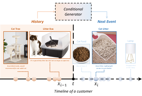
Figure 1: An example of generating high-dimensional content over time. In this example, the conditional generator explores the customer’s next possible activity, including not only the purchase time, but also the item, and even its image or review. The observed events from the customer’s past purchases are represented by yellow dots, while the next generated event is indicated by a blue dot.

To address the above challenges, this paper presents a novel generative framework for modeling point processes with high-dimensional marks and generating high-quality events based on observed history, leveraging recent developments in generative modeling [13, 19, 40]. The effectiveness of generative models is rooted in their ability to approximate the underlying high-dimensional data distribution through generated samples, rather than directly estimating the density function. In our framework, unlike traditional point process models that depend on defining the conditional intensity or probability density function [6, 8, 25, 37], our model estimates the distribution of events using samples generated by a conditional generator. The event generator takes the history of events as its input, which can be summarized by a recurrent neural architecture or other flexible selections based on the application’s needs. An illustrative example is shown in Figure 1. By doing so, we can approximate the point process likelihood using generated events without involving numerical approximations during the model learning. Meanwhile, instead of relying on the sampling-rejection procedure in the thinning algorithm, we can directly simulate future events that conform to the underlying conditional event distribution, which is learned by the conditional event generator. In general, the benefits of our model can be summarized by:

1. Our model is capable of handling high-dimensional marks such as images or texts, an area not extensively delved into in prior marked point process research;

2. Our model excels in computational efficiency during both the training phase and the event generation process.

3. Our model possesses superior representative power, as it does not confine the conditional intensity or probability density of the point process to any specific parametric form;

4. Our model outperforms existing state-of-the-art baselines in terms of estimation accuracy and generating high-quality event series;

It is important to note that our proposed framework is general and model-agnostic, meaning that a wide spectrum of generative models and learning algorithms can be applied within our framework. In this paper, we present two possible learning algorithms and evaluate our framework through extensive numerical experiments on both synthetic and real-world data sets.

1.1 Related work

Seminal works in point processes [11, 30] introduce self-exciting conditional intensity functions with parametric kernels. While these models have proven useful, they possess limitations in capturing the intricate patterns observed in real-world applications. Landmark studies about neural point processes like recurrent marked temporal point processes (RMTPP) [8] and Neural Hawkes [25] have leveraged recurrent neural networks (RNNs) to embed event history into a hidden state, which then represents the conditional intensity function. Another line of research opts for a more “parametric” way, which only replaces the parametric kernel in the conditional intensity using neural networks [7, 31, 52, 55]. However, these methods can be computationally inefficient, and even intractable, when dealing with multi-dimensional marks due to the need for numerical integration. Alternative approaches have been proposed by other studies [4, 32, 36, 51] to overcome the challenges, focusing on modeling the cumulative hazard function or conditional probability rather than the conditional intensity, thereby eliminating the need for integral calculations. Nonetheless, these methods are typically used for low-dimensional event data, and still rely on the thinning algorithm for simulating or generating event series, which significantly limits their applicability in modern applications. Some studies [6, 54] propose to model high-dimensional marks by considering simplified finite mark space. However, work on handling high-dimensional marks in point processes is still limited.

Our research paper is closely connected to the field of generative modeling, which aims to generate high-quality samples from learned data distributions. Prominent examples of generative models include generative adversarial networks (GANs) [9], variational autoencoders (VAEs) [19], and diffusion models [13, 38, 42]. Recent studies have introduced conditional generative models [14, 26, 40] that can generate diverse and well-structured outputs based on specific input information. In our work, we adopt a similar technique where we consider the history of observed events as contextual information to generate high-quality future events. Furthermore, more recent advancements in this field [2, 21] have extended the application of conditional generative models to a broader range of settings such as reinforcement learning.

The application of generative models to point processes has received limited attention in the literature. Three influential papers [22, 35, 46] have made significant contributions in this area by using RNN-like models to generate future events. While RNNs are commonly used for prediction, these papers assume the model’s output follows a Gaussian distribution, enabling the exploration of the event space, albeit at the cost of limiting the representational power of the models. To learn the model, they choose to minimize the “similarity” (e.g., Maximum Mean Discrepancy or Wasserstein distance) between the generated and the observed event sequences. It is important to note that these metrics are designed to measure the discrepancy between two distributions in which each data point is assumed to be independent of the others. This approach may not always be applicable to temporal point processes, particularly when the occurrence of future events depends on the historical context. A similar concept of modeling point processes using conditional generative models is also explored in another concurrent paper [23, 49]. However, their approaches differ from ours in terms of the specific architecture used. They propose a diffusion model with an attention-based encoder, while our framework remains model-agnostic, allowing for greater flexibility in selecting different models. Additionally, their works primarily focus on one-dimensional or spatio-temporal events, and do not account for multi- or high-dimensional marks.

2 Methodology

2.1 Background: Marked temporal point processes

Marked temporal point processes (MTPPs) [33] consist of a sequence of discrete events over time. Each event is associated with a (possibly multi-dimensional) mark that contains detailed information of the event, such as location, nodal information (if the observations are over networks, such as sensor or social networks), and contextual information (such as token, image, and text descriptions). Let $T>0$ be a fixed time-horizon, and $\mathcal{M}\subseteq\mathbb{R}^{d}$ be the space of marks. We denote the space of observation as $\mathcal{X}=[0,T)\times\mathcal{M}$ and a data point in the discrete event sequence as

$$x=(t,m),\quad t\in[0,T),\quad m\in\mathcal{M},$$

where $t$ is the event time and $m$ represents the mark. Let $N_{t}$ be the number of events up to time $t<T$ (which is random), and $\mathcal{H}_{t}:=\{x_{1},x_{2},\dots,x_{N_{t}}\}$ denote historical events. Let $\mathbb{N}$ be the counting measure on $\mathcal{X}$, i.e., for any measurable $S\subseteq\mathcal{X}$, $\mathbb{N}(S)=|\mathcal{H}_{t}\cap S|.$ For any function $\phi:\mathcal{X}\to\mathbb{R}$, the integral with respect to the counting measure is defined as

$$\int_{S}\phi(x)d\mathbb{N}(x)=\sum_{x_{i}\in\mathcal{H}_{T}\cap S}\phi(x_{i}).$$

The events’ distribution in MTPPs can be characterized via the conditional intensity function $\lambda$, which is defined to be the occurrence rate of events in the marked temporal space $\mathcal{X}$ given the events’ history $\mathcal{H}_{t(x)}$, i.e.,

$$\lambda(x|\mathcal{H}_{t(x)})=\mathbb{E}\left(d\mathbb{N}(x)|\mathcal{H}_{t(x)}\right)/dx,$$ (1)

where $t(x)$ extracts the occurrence time of the possible event $x$. Given the conditional intensity function $\lambda$, the corresponding conditional probability density function (PDF) can be written as

$$f(x|\mathcal{H}_{t(x)})=\lambda(x|\mathcal{H}_{t(x)})\cdot\exp\left(-\int_{[t_{n},t(x))\times\mathcal{M}}\lambda(u|\mathcal{H}_{t(u)})du\right).$$ (2)

where $t_{n}$ denotes the time of the most recent event that occurred before time $t(x)$.

Maximum likelihood estimation (MLE) has been the commonly used approach for learning the point process models. The log-likelihood of observing a sequence with $N_{T}$ events can be expressed in terms of $\lambda$ by the product rule of conditional probability as

$$\ell(x_{1},\dots,x_{N_{T}})=\int_{\mathcal{X}}\log\lambda(x|\mathcal{H}_{t(x)})d\mathbb{N}(x)-\int_{\mathcal{X}}\lambda(x|\mathcal{H}_{t(x)})dx.$$ (3)

See all the derivations in Appendix A. Previous methods aim to find the appropriate modeling of $\lambda$ or $f$ for downstream tasks such as event prediction and generation, while our approach goes beyond the explicit parametrization of $\lambda$ or $f$, as illustrated in the next part.

2.2 Conditional event generator

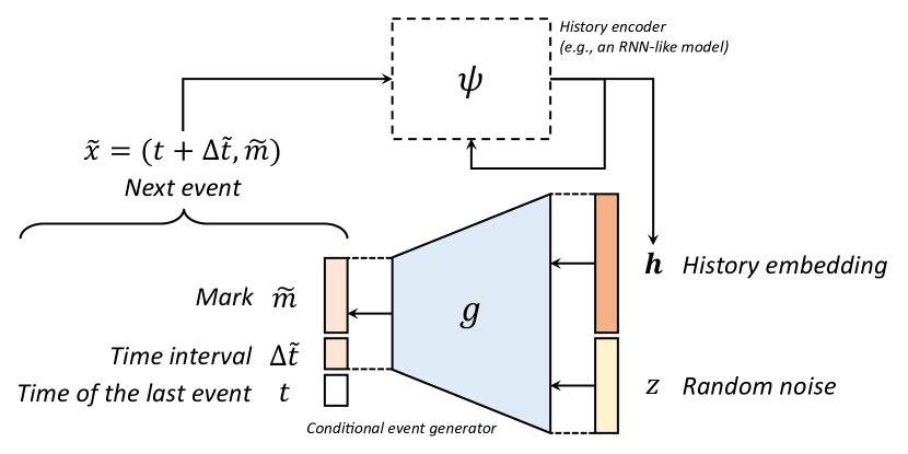
(a) Model architecture

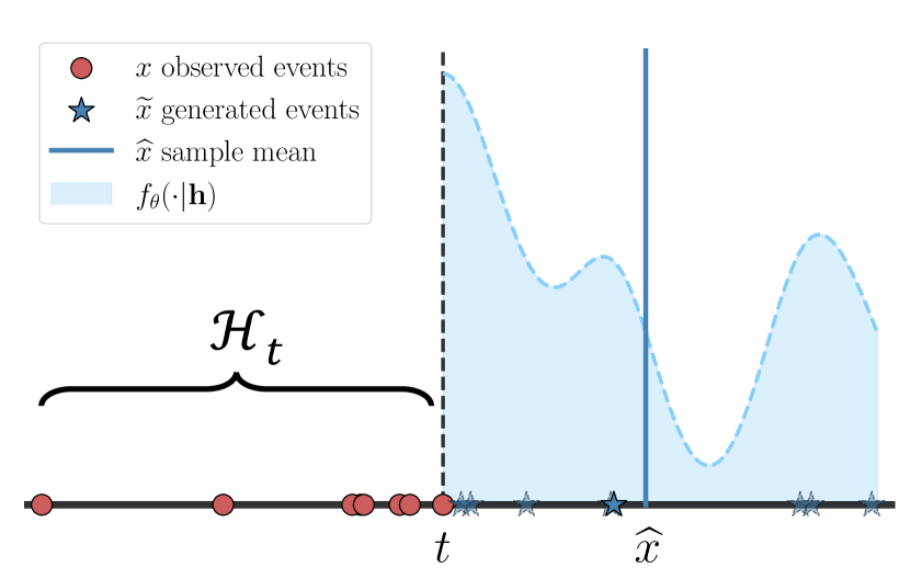
(b) Example of generated events

Figure 2: (a) The architecture of the proposed framework, which consists of two key components: A conditional generative model $g$ that generates $(\Delta\widetilde{t},\widetilde{m})$ given its history embedding and an RNN-like model $\psi$ that summarizes the events in the history. (b) An example of generated one-dimensional (time only) events $\{\widetilde{x}^{(j)}\}$ given the history $\mathcal{H}_{t}$. The shaded area suggests the underlying conditional probability density captured by the model parameters $\theta$.

The main idea of the proposed framework is to use a conditional event generator (CEG) to produce the $i$-th event $x_{i}=(t_{i-1}+\Delta t_{i},m_{i})$ given its previous $i-1$ events, without relying on $\lambda$ or $f$. Here, $\Delta t_{i}$ and $m_{i}$ indicate the time interval between the $i$-th event and its preceding event and the mark of the $i$-th event, respectively. Formally, this is achieved by a generator function:

$$g(z,\bm{h}_{i-1}):\mathbb{R}^{r+p}\to(0,+\infty)\times\mathcal{M},$$ (4)

which takes an input in the form of a random noise vector ($z\in\mathbb{R}^{r}\sim\mathcal{N}(0,I)$) and a history embedding ($\bm{h}_{i-1}\in\mathbb{R}^{p}$) that summarizes the history information up to and excluding the $i$-th event, namely, $\mathcal{H}_{t_{i}}=\{x_{1},\dots,x_{i-1}\}$. The output of the generator includes the event time interval and the mark of the $i$-th event denoted by $\Delta\widetilde{t}_{i}$ and $\widetilde{m}_{i}$, respectively. To ensure that the time interval is positive, we restrict $\Delta\widetilde{t}_{i}$ to be greater than zero. It is worth noting that our selection of the generator $g$ is not constrained to a particular function. Instead, it can represent an arbitrary generative process, such as a diffusion model, provided it has the capability to produce a sample when supplied with noise and a history embedding.

To represent the conditioning variable $\bm{h}_{i-1}$, we use a history encoder represented by $\psi$, which has a recursive structure such as recurrent neural networks (RNNs) [48] or Transformers [43]. In our numerical results, we opt for long short-term memory (LSTM) [10], which takes the current event $x_{i}$ and the preceding history embedding $\bm{h}_{i-1}$ as input and generates the new history embedding $\bm{h}_{i}$. This new history embedding represents an updated summary of the past events including $x_{i}$. Formally,

$$\bm{h}_{0}=\bm{0}\leavevmode\nobreak\ \text{and}\leavevmode\nobreak\ \bm{h}_{i}=\psi(x_{i},\bm{h}_{i-1}),\quad i=1,2,\dots,N_{T}.$$

We denote the parameters of both models $g$ and $\psi$ using $\theta\in\Theta$. The model architecture is presented in Figure 2 (a).

Connection to marked temporal point processes

The proposed framework draws its statistical inspiration from MTPPs. Unlike other recent attempts at modeling point processes, our framework approximates the conditional probability of events using generated samples rather than directly modeling the conditional intensity in (1) or PDF in (2) [8, 25, 32, 36, 53, 56].

Let $\bm{h}$ denote the history embedding of $\mathcal{H}_{t}$. Given $\bm{h}$, our model generates the subsequent event occuring after $t$, denoted by $\widetilde{x}=(t+\Delta\widetilde{t},\widetilde{m})$. The generated event adheres to the following conditional probabilistic distribution:

$$\widetilde{x}\sim f_{\theta}(\cdot|\bm{h})\approx f(\cdot|\mathcal{H}_{t}),$$

where $f_{\theta}$ denotes the conditional PDF of the underlying MTPP model (2). This design has three main advantages compared to other point process models:

1. Generative efficiency: Our model’s generative capability enables highly efficient simulation of event series for any point processes without the need for thinning algorithms [29]. Thinning algorithms typically generate a large number of random samples ($\mathcal{O}(N^{d})$) across a high-dimensional space, only to retain a small portion of them ($\mathcal{O}(N_{T})$) based on predicted conditional intensity, where $N_{T}\ll N^{d}$. Our method, however, bypasses this by directly generating samples through CEG (Algorithm 1), significantly reducing complexity from $\mathcal{O}(N^{d})$ to $\mathcal{O}(N_{T})$, eliminating the inefficiency incurred by the sample rejection.

2. Expressiveness: The proposed model enjoys considerable representational power, as it does not impose any restrictions on the parametric form of the conditional intensity $\lambda$ or PDF $f$. The numerical findings also indicate that our model is capable of capturing complex event interactions, even in a multi-dimensional space.

3. Predictive efficiency: To predict the next event $\widehat{x}_{i}=(t_{i-1}+\Delta\widehat{t}_{i},\widehat{m}_{i})$ given the observed events’ history $\mathcal{H}_{t_{i}}$, we can calculate the sample average over a set of generated events $\{\widetilde{x}_{i}^{(l)}\}$ without the need for an explicit expectation computation, i.e.,

   $$\widehat{x}_{i}=\int_{(t_{i-1},+\infty)\times\mathcal{M}}x\cdot f(x|\mathcal{H}_{t(x)})dx\approx\frac{1}{L}\sum_{l=1}^{L}\leavevmode\nobreak\ \widetilde{x}_{i}^{(l)},$$

   where $L$ denotes the number of samples.

  Input: Generator $g$, history encoder $\psi$, time horizon $T$ 

  Initialization: $\mathcal{H}_{T}=\emptyset,\bm{h}_{0}=\bm{0},t=0,i=0$ 

  while $t<T$ do

     1. Sample $z\sim\mathcal{N}(0,I)$;

     2. Generate next event $\widetilde{x}=(t+\Delta\widetilde{t},\widetilde{m})$, where $(\Delta\widetilde{t},\widetilde{m})=g(z,\bm{h}_{i})$;

     3. $i=i+1$; $t=t+\Delta\widetilde{t};x_{i}=\widetilde{x}$; $\mathcal{H}_{T}=\mathcal{H}_{T}\cup\{x_{i}\}$;

     4. Update history embedding $\bm{h}_{i}=\psi(x_{i},\bm{h}_{i-1})$;

  end while

  if $t(x_{i})\geq T$ then

     return $\mathcal{H}_{T}-\{x_{i}\}$  

  else

     return $\mathcal{H}_{T}$  

  end if

Algorithm 1 Event generation process using CEG

  Input: noise $z_{K}\sim\mathcal{N}(0,I)$, history embedding $\bm{h}$ 

  for $k=K,\dots,1$ do

     1. Sample $\epsilon\sim\mathcal{N}(0,I)$ if $k>1$, else $\epsilon=0$;

     2. $\tilde{\epsilon}=(1+w)\epsilon_{\theta}(z_{k},\bm{h},k)-w\epsilon_{\theta}(z_{k},\varnothing,k)$, where $w$ is the pre-chosen guidance strength;

     3. $z_{k-1}=\frac{1}{\sqrt{\alpha_{t}}}\left(z_{k}-\frac{1-\alpha_{t}}{\sqrt{1-\bar{\alpha}_{t}}}\tilde{\epsilon}\right)+\sqrt{\beta}_{t}\epsilon$;

  end for

  return $\widetilde{x}\coloneqq z_{0}$  

Algorithm 2 Generator $g$ in CDDM with classifier-free guidance

2.3 Model estimation

To learn the model, one can maximize the log-likelihood of the observed event series. Instead of directly specifying the log-likelihood using $\lambda$ as in (3), an equivalent form of this objective can be expressed using conditional PDF, as shown in the following equation (see Appendix A for the derivation):

$$\max_{\theta\in\Theta}\leavevmode\nobreak\ \ell(\theta)\coloneqq\frac{1}{E}\sum_{e=1}^{E}\int_{\mathcal{X}}\leavevmode\nobreak\ \log f_{\theta}(x|\bm{h})\leavevmode\nobreak\ d\mathbb{N}_{e}(x),$$ (5)

where $E$ represents the total number of observed event sequences and $\mathbb{N}_{e}$ is the counting measure of the $e$-th event sequence. Therefore, The log-likelihood (3) is the summation of the log conditional probabilistic density function $f_{\theta}$ evaluated at all events. It is worth noting that this learning objective circumvents the need to compute the intensity function and its integral in the second term of (3), a task that can be computationally intractable when events exist in a multi- or high-dimensional data space.

Now the key challenge is how do we maximize the model likelihood without access to the function $f_{\theta}$? This is a commonly posed inquiry in the realm of generative model learning, and there are several pre-existing learning algorithms intended for generative models that can provide solutions to this question [3]. In the rest of this section, we present the learning strategy of denoising score matching by choosing a conditional diffusion model as the CEG in our framework. In this way, a denoising process is assumed to transform a noise distribution to the real data distribution, and we can use the generated samples to match the denoising scores of this process through a score function parametrized by a neural network, therefore maximizing the log-likelihood of the real data [13, 41]. Other learning algorithms for likelihood maximization can also be adopted, and we provide two additional approaches in Appendix B and C, which serves as ablation study in our experiments.

Conditional denoising diffusion model.

For ease of presentation, we only consider the conditional PDF of a single event $x$ in the following derivation. The conditional denoising diffusion model (CDDM) approximates the data distribution in the form of $f_{\theta}(x|\bm{h})\coloneqq\int p_{\theta}(x,z_{1:K}|\bm{h})dz_{1:K}$, where $z_{1:K}$ are latent variables of the same dimensionality as the data $x$ and $p_{\theta}$ is the model to be learned. The variational distribution of the latent variables $q(z_{1:K}|x,\bm{h})$ is assumed by a forward process, which is fixed to a Markov chain to gradually add noise to the data $x$ with variance schedule $\{\beta_{k}\}_{k=1}^{K}$. Another reverse process inverts the transformation from the noise distribution $\mathcal{N}(0,I)$ back to data, with Gaussian transitions parametrized by the model parameters $\theta$. The model can be learned by maximizing the variational bound on the log-likelihood of the data $x$:

$$\log f_{\theta}(x|\bm{h}) \geq\mathbb{E}_{q}\left[\log p(z_{K}|\bm{h})+\log\frac{p_{\theta}(x|z_{1},\bm{h})}{q(z_{1}|x,\bm{h})}+\sum_{k>1}\log\frac{p_{\theta}(z_{k-1}|z_{k},\bm{h})}{q(z_{k}|z_{k-1},\bm{h})}\right].$$

The variational bound can be expressed by the KL divergence between a series of Gaussian distributions of $z_{1:K}$ and $x$, leading to the following equivalent objective:

$$\mathbb{E}_{q}\left[\sum_{k>1}\frac{1}{2\beta_{k}}\|\tilde{\mu}_{k}(z_{k},x)-\mu_{\theta}(z_{k},k|\bm{h})\|^{2}\right]+C,$$

where $\mu_{\theta}$ is the mean function of the Gaussian transitions to be learned. The $\tilde{\mu}_{k}$ is the mean of forward process posteriors for the reverse process to match, with $\tilde{\mu}_{k}(z_{k},x)=\frac{\sqrt{\bar{\alpha}_{k-1}}\beta_{k}}{1-\bar{\alpha}_{k}}x+\frac{\sqrt{\alpha_{k}}(1-\bar{\alpha}_{k-1})}{1-\bar{\alpha}_{k}}z_{k}$, $\alpha_{k}\coloneqq 1-\beta_{k},\bar{\alpha}_{k}\coloneqq\prod_{r=1}^{k}\alpha_{r}$, and $C$ is a constant that does not depend on $\theta$. Using $\epsilon$-prediction [13], we can finally train the model by

$$\min_{\theta\in\Theta}\leavevmode\nobreak\ \mathbb{E}_{k,\epsilon}\left[\|\epsilon-\epsilon_{\theta}(\sqrt{\bar{\alpha}_{k}}x+\sqrt{1-\bar{\alpha}_{k}}\epsilon,\bm{h},k)\|^{2}\right].$$ (6)

The $\epsilon_{\theta}$ is the score function parametrized by a neural network for denoising score matching, and the learned score $\epsilon_{\theta}(\sqrt{\bar{\alpha}_{k}}x+\sqrt{1-\bar{\alpha}_{k}}\epsilon,\bm{h},k)$ estimates the gradient of the log-density of the conditional distribution of $z_{k}$ using generated samples. The final loss function is composed of the score-matching loss at all observed events (i.e., summing (6) over $x$ and corresponding $\bm{h}$).

We choose the classifier-free diffusion guidance [14] to achieve the conditional sampling using the denoising diffusion model. By incorporating this model architecture, the generator function $g$ is chosen to be the entire reverse process for sampling data from any given noise, as illustrated in Algorithm 2. See Appendix D for derivation and implementation details of training and sampling.

3 Experiments

We evaluate our method using both synthetic and real data and demonstrate the superior performance compared to five state-of-the-art approaches, including (1) Recurrent marked temporal point processes (RMTPP) [8], (2) Neural Hawkes (NH) [25], (3) Fully neural network based model (FullyNN) [32], (4) Epidemic type aftershock sequence (ETAS) [30] model, (5) Deep non-stationary kernel in point process (DNSK) [6]. The first three baselines leverage neural networks to model temporal event data (or only with categorical marks). The last two baselines are chosen for testing multi- and high-dimensional event data. Meanwhile, the DNSK is the state-of-the-art method that uses neural networks for high-dimensional mark modeling. See [37] and Appendix F for a detailed review of these baseline models. In the following, we demonstrate the effectiveness of our conditional event generator as a conditional denoising diffusion model (CEG+CDDM), as well as another two variants with the event generator being a fully-connected neural network (CEG+KDE, see Appendix B) or a conditional variational auto-encoder (CEG+CVAE, see Appendix C). Details about the experimental setup and our model architecture are presented in Appendix F.

Table 1: Performance comparison with five baseline methods (bold indicates the best performance).

	1D self-exciting data			1D self-correcting data			3D synthetic data			3D earthquake data
Model	Testing $\ell$ ($\uparrow$)	MRE of $f$ ($\downarrow$)	MRE of $\lambda$ ($\downarrow$)	Testing $\ell$	MRE of $f$	MRE of $\lambda$	Testing $\ell$	MRE of $f$	MRE of $\lambda$	Testing $\ell$
RMTPP	$-1.051\leavevmode\nobreak\ (0.015)$	$0.437$	$0.447$	$-0.975\leavevmode\nobreak\ (0.006)$	$0.308$	$0.391$	/	/	/	/
NH	$-0.776\leavevmode\nobreak\ (0.035)$	$0.175$	$0.198$	$-1.004\leavevmode\nobreak\ (0.010)$	$0.260$	$0.363$	/	/	/	/
FullyNN	$-0.729\leavevmode\nobreak\ (0.003)$	$0.083$	$0.105$	$-0.821\leavevmode\nobreak\ (0.008)$	$0.121$	$0.167$	/	/	/	/
ETAS	/	/	/	/	/	/	$-4.832\leavevmode\nobreak\ (0.002)$	$0.981$	$0.902$	$-3.939\leavevmode\nobreak\ (0.002)$
DNSK	$-0.649\leavevmode\nobreak\ (0.002)$	$0.015$	0.024	$-2.832\leavevmode\nobreak\ (0.004)$	$0.134$	$0.185$	$-2.560\leavevmode\nobreak\ (0.004)$	$0.339$	$0.415$	$-3.606\leavevmode\nobreak\ (0.003)$
CEG+KDE	$\textbf{--0.645}\leavevmode\nobreak\ (0.002)$	0.013	$0.066$	$\textbf{--0.768}\leavevmode\nobreak\ (0.005)$	0.042	0.075	$-2.540\leavevmode\nobreak\ (0.011)$	$0.056$	$0.101$	$-2.629\leavevmode\nobreak\ (0.015)$
CEG+CVAE	$-0.702\leavevmode\nobreak\ (0.006)$	$0.073$	$0.102$	$-0.941\leavevmode\nobreak\ (0.010)$	$0.165$	$0.379$	$-2.558\leavevmode\nobreak\ (0.009)$	$0.093$	$0.156$	$-3.505\leavevmode\nobreak\ (0.023)$
CEG+CDDM	$-0.691\leavevmode\nobreak\ (0.004)$	$0.067$	$0.089$	$-0.775\leavevmode\nobreak\ (0.003)$	$0.117$	$0.187$	$\textbf{--2.501}\leavevmode\nobreak\ (0.008)$	0.042	0.097	$\textbf{--0.299}\leavevmode\nobreak\ (0.006)$

• *Numbers in parentheses present standard error for three independent runs.

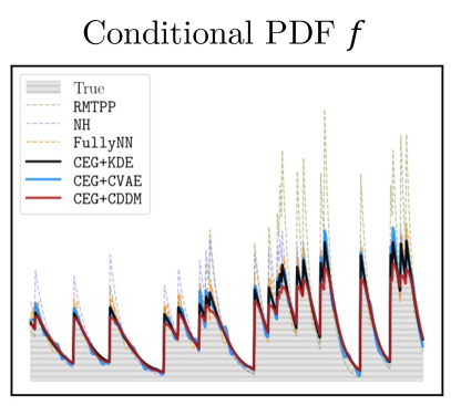
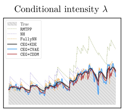
(a) One sequence from self-exciting data

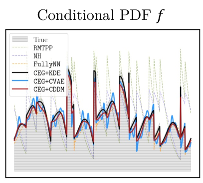
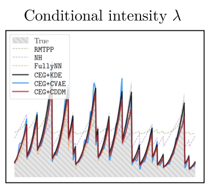
(b) One sequence from self-correcting data

Figure 3: Out-of-sample estimation of the conditional PDF $f(t|\mathcal{H}_{t})$ and the corresponding intensity $\lambda(t|\mathcal{H}_{t})$ by each model on one-dimensional (time only) synthetic data sets. One testing sequence is picked from each dataset. The grey shaded areas with horizontal texture represent the true $f(t|\mathcal{H}_{t})$, and those with diagonal texture represent the true $\lambda(t|\mathcal{H}_{t})$.

3.1 Synthetic data

We first evaluate our model on synthetic data, aiming to showcase its ability to accurately recover the conditional distribution or intensity from the observed events. To be specific, we generate two one-dimensional (1D) and a three-dimensional (3D) synthetic data sets: Each synthetic data set includes 1,000 sequences, with an average length of 150 events per sequence. Two 1D (time-only) data sets are simulated by a self-exciting process and a self-correcting process, respectively, using the thinning algorithm (Algorithm 6 in Appendix F). The 3D (time and space) data set is generated by a randomly initialized CEG+KDE using Algorithm 1.

To assess the effectiveness of our model, we incorporate three quantitative metrics for the evaluations on synthetic data sets: mean relative error (MRE) of the estimated conditional intensity and PDF compared to the ground truth on one randomly selected testing sequence, and the model log-likelihood on the entire testing set. Note that we obtain these metrics for our model and other baselines in different ways. For our model, we first estimate the conditional PDF using generated samples, and then follow Appendix A and (5) to calculate the intensity function and model likelihood, respectively. For the baselines, we need first to estimate the conditional intensity function based on their models and then compute the corresponding conditional PDF and log-likelihood by numerical approximations using (2) and (3), respectively.

Figure 3 shows the estimated conditional PDFs and intensities, as well as their corresponding ground truth on one testing sequence from each 1D data set. The sequence in the left column is generated by the self-exciting process, and the one in the right column is generated by the self-correcting process. The results in the four panels show that all three variants of our generative model enjoy superior performance compared to other baseline models in accurately recovering the true conditional PDFs and intensities for both data sets. Table 1 presents results regarding the quantitative metrics on 1D and 3D data sets, including the log-likelihood per testing event and the mean relative error (MRE) of the recovered conditional density and intensity. These results demonstrate the consistent comparable or superior performance of CEG against other methods across all scenarios. Note that CEG+KDE has achieved the best scores among three variants of our model on both 1D synthetic data sets. However, the accurate estimation of the conditional PDF using KDE (Appendix B) in multi-dimensional spaces requires numerous samples generated from the model, thus incurring larger estimation errors (e.g., seeing the results on 3D synthetic and real earthquake data) and making the learning extremely expensive or even infeasible when in high-dimensional spaces. Figure F3 in Appendix F presents results of the estimated conditional probability density on the 3D synthetic data set, where CEG+CDDM accurately captures the complex spatio-temporal point patterns while DNSK and ETAS fail to do so. These results on synthetic data sets not only demonstrate the exceptional performance of our framework but also indicate the necessity of model flexibility to integrate various model architectures based on practical needs.

3.2 Semi-synthetic data with image marks

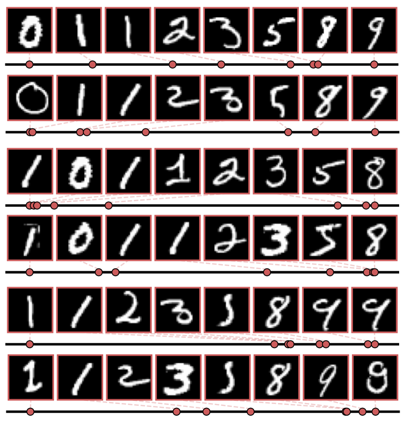
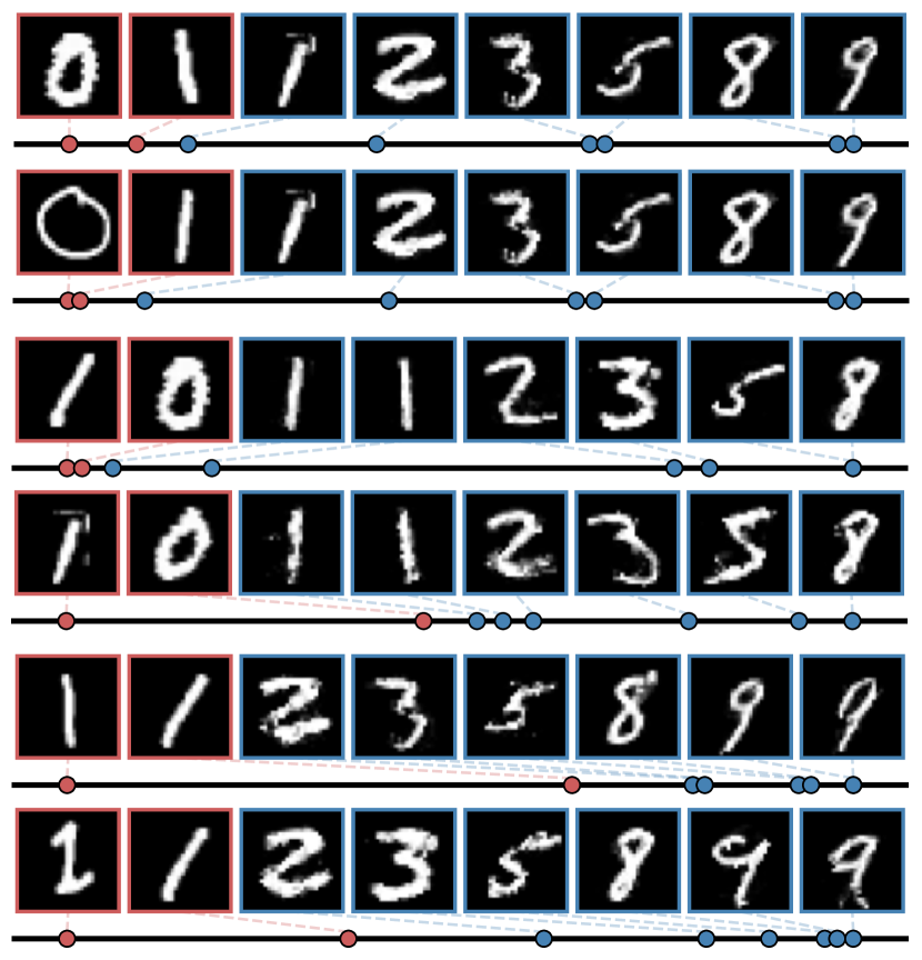
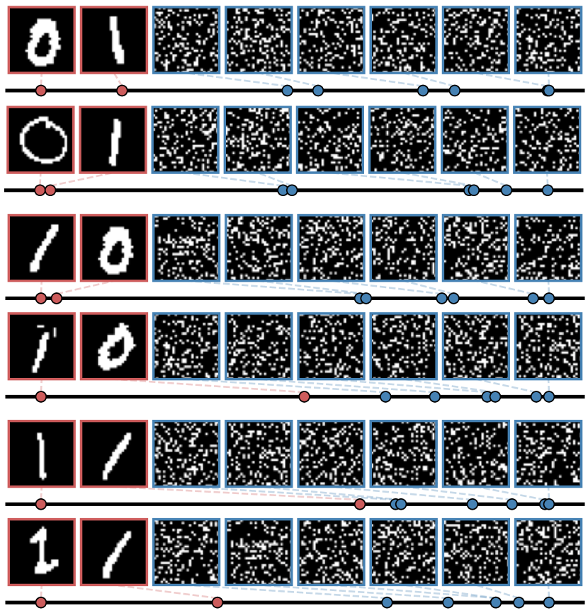
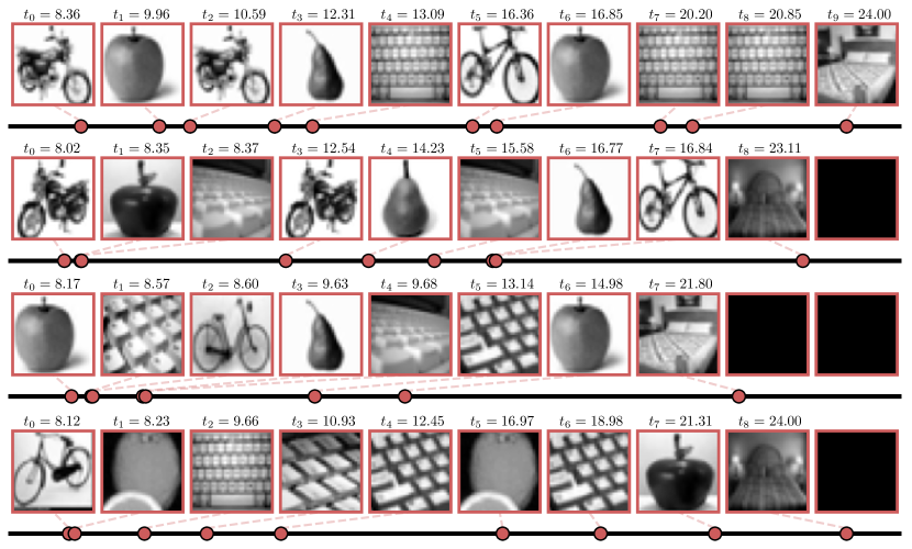
(a) True series

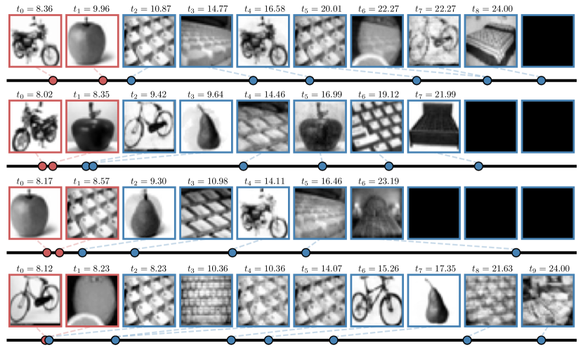
(b) CEG generated series

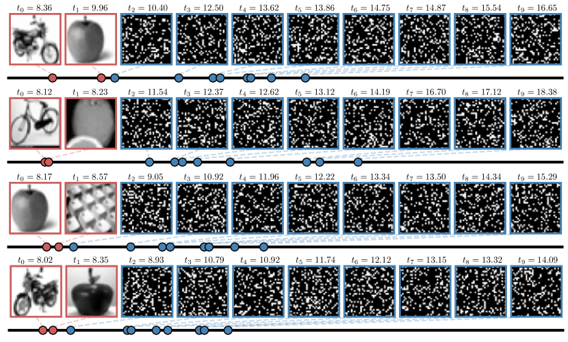
(c) DNSK generated series

Figure 4: Generated T-MNIST (first row) and T-CIFAR (second row) series using CEG and a neural point process baseline DNSK, with true sequences displayed on the left. Each event series is generated (blue boxes) given the first two true events (red boxes). Dots on the horizontal lines represent the event times, with the dashed lines indicating the association between time and mark.

We test our model’s capability of generating complex high-dimensional marked events on two semi-synthetic data, including time-stamped MNIST (T-MNIST) and CIFAR-100 (T-CIFAR). In these data sets, both the mark (the image category) and the timestamp are generated through a marked point process. Images from MNIST and CIFAR-100 are subsequently chosen at random based on these marks, acting as a high-dimensional representation of the original image category. It’s important to note that during the training phase, categorical marks are excluded, retaining only the high-dimensional images for model learning. Details of the data generation processes can be found in Appendix F.

1. T-MNIST: For each sequence in the data, the actual digit in the succeeding image is the aggregate of the digits in the two preceding marks. The initial two digits are randomly selected from $0$ and $1$. The digits in the marks must be less than nine. The hand-written image for each mark is then chosen from the corresponding subset of MNIST according to the digit. The time for the entire MNIST series conforms to a Hawkes process with an exponentially decaying kernel.

2. T-CIFAR: The data contains event series that depict a typical day in the life of a graduate student, spanning from 8:00 to 24:00. The marks are sampled from four categories: outdoor exercises, food ingestion, working, and sleeping. Depending on the most recent activity, the subsequent one is determined by a transition probability matrix. Images are selected from the respective categories to symbolize each activity. The time for these activities follows a self-correcting process.

Evaluation of the high-dimensional data sets.

Since evaluating the log-likelihood for event series with high-dimensional marks is infeasible for our model (the number of samples needed to estimate the density function at one data point is impractically large), we evaluate the model performance according to (i) the quality of the generated event time sequences, (ii) the quality of the generated image marks, and (iii) the transition dynamics of the entire series. For (i), we use the predictive score (Pred.) and the discriminative score (Disc.) proposed in [47] for measuring the fidelity and diversity of the synthesized time-series samples (See more details about these two metrics in Appendix F). For (ii), we do not include the FID [12] or IS [34] because we are not focusing on the image generation problem, and the quality difference of the generated image marks from different models can be easily distinguished. Here, we compared our model CEG+CDDM only with DNSK, since other baselines cannot handle high-dimensional event marks.

Figure 4 presents the true T-MNIST series alongside the series generated by CEG and DNSK given the first two events. Our model not only generates high-dimensional event marks that resemble true images, but also successfully captures the underlying data dynamics, such as the clustering patterns of the self-exciting process and the transition pattern of image marks. On the contrary, the DNSK only learns the temporal effects of historical events and struggles to estimate the conditional intensity for the high-dimensional marks. The metrics presented in Table 2 also suggest that our model outperforms DNSK by a large margin, by quantitatively measuring the quality of the generated event time sequences compared with the training data. Besides, the grainy images generated by DNSK demonstrate the challenge of simulating credible high-dimensional content using the thinning algorithm, thus limiting the usefulness of previous approaches in such an application. This is because the real data points, being sparsely scattered in the high-dimensional mark space, make it challenging for the candidate points to align closely with them in the thinning algorithm.

Similar results are shown in Figure 4 and Table 2 on T-CIFAR data, where CEG is able to simulate high-quality daily activities with high-dimensional content at appropriate times. However, DNSK fails to extract any meaningful patterns from data, since intensity-based modeling or data generation become ineffectual in high-dimensional mark space.

Table 2: Quantitative evaluation of the generated event time sequences with high-dimensional marks.

	T-MNIST		T-CIFAR		Textual crime
Model	Disc.($\downarrow$)	Pred.($\downarrow$)	Disc.	Pred.	Disc.	Pred.
DNSK	$0.388\leavevmode\nobreak\ (0.021)$	$\textbf{0.003}\leavevmode\nobreak\ (0.001)$	$0.375\leavevmode\nobreak\ (0.050)$	$0.031\leavevmode\nobreak\ (0.002)$	$0.500\leavevmode\nobreak\ (0.000)$	$0.010\leavevmode\nobreak\ (0.008)$
CEG+CDDM	$\textbf{0.063}\leavevmode\nobreak\ (0.034)$	$\textbf{0.003}\leavevmode\nobreak\ (<0.001)$	$\textbf{0.168}\leavevmode\nobreak\ (0.027)$	$\textbf{0.006}\leavevmode\nobreak\ (<0.001)$	$\textbf{0.071}\leavevmode\nobreak\ (0.014)$	$\textbf{0.002}\leavevmode\nobreak\ (<0.001)$

• *Numbers in parentheses present standard error for five independent runs.

3.3 Real data

In our real data results, our model also demonstrates superior efficacy in generating high-quality multi- or high-dimensional event sequences, using earthquake and crime data sets.

Northern California earthquake catalog.

We test our method using the Northern California Earthquake Data [28], which contains detailed information on the timing and location of earthquakes that occurred in central and northern California from 1978 to 2018, totaling 5,984 records with magnitude greater than 3.5. We divided the data into several sequences by month. In comparison to other baseline methods that can only handle 1D event data, we primarily evaluated our model against DNSK and ETAS, training each model using 80% of the dataset and testing them on the rest. To demonstrate the effectiveness of our method on the real data, we assess the quality of the generated sequences by each model. Our model’s generation process for new sequences can be efficiently carried out using Algorithm 1, whereas both DNSK and ETAS requires the use of a thinning algorithm (Algorithm 6) for simulation. We also compared the estimated conditional probability density functions (PDFs) of real sequences by each model in Appendix F.

We compare the generative ability of each method in Figure 5. The top left sub-figure features a single event series selected at random from the data set, while the rest of the sub-figures in the first row exhibit event series generated by each model, respectively. The quality of the generated earthquake sequence using our method is markedly superior to that generated by DNSK and ETAS. We also simulate multiple sequences using each method and visualize the spatial distribution of generated earthquakes in the second row. The shaded area reflects the spatial density of earthquakes obtained by KDE and represents the “background rate” over space. It is evident that CEG is successful in capturing the underlying earthquake distribution, while the two STPP baselines are unable to do so. Additional results in Figure F5 visualizes the conditional PDF estimated by CEG, DNSK, and ETAS for an actual earthquake sequence in testing set, respectively. The results indicate that our model is able to capture the heterogeneous triggering effects among earthquakes which align with current understandings of the San Andreas Fault System [44]. However, both DNSK and ETAS fail to extract this geographical feature from the data.

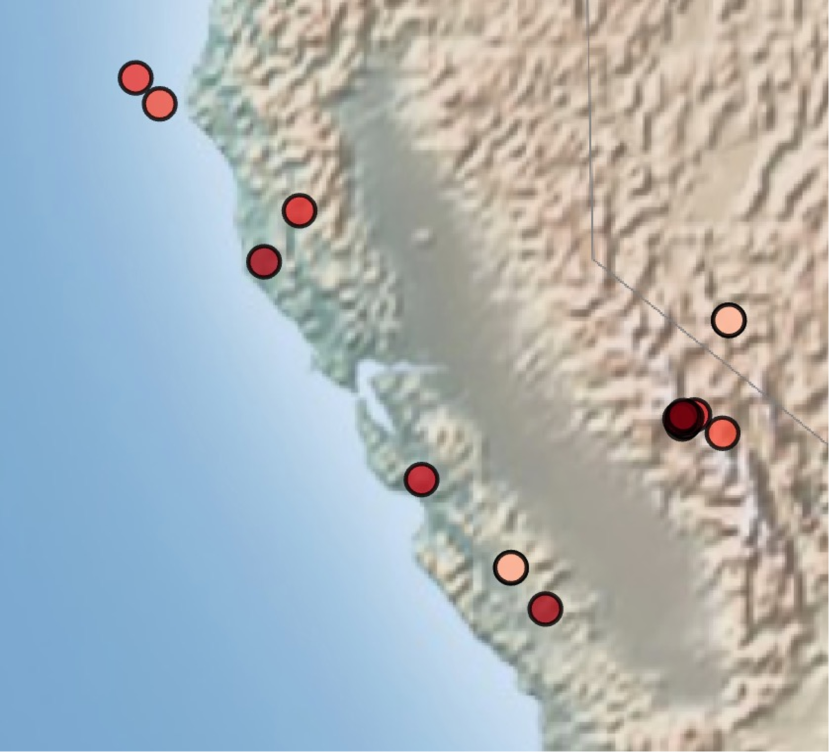
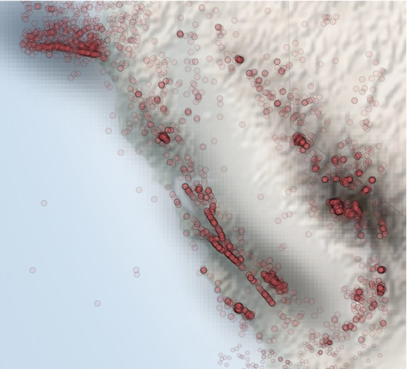
(a) Real

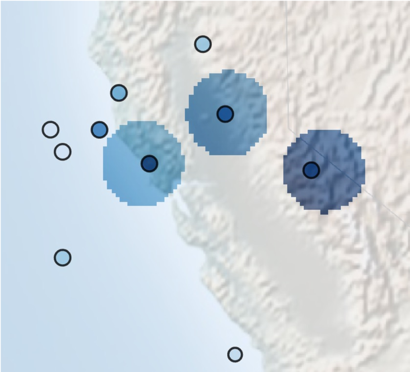
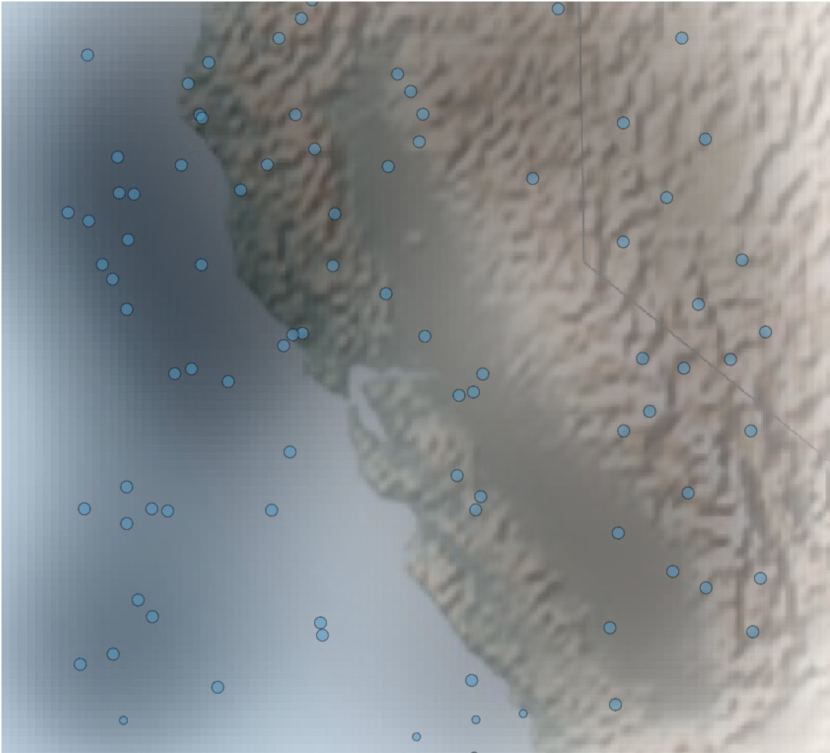
(b) DNSK

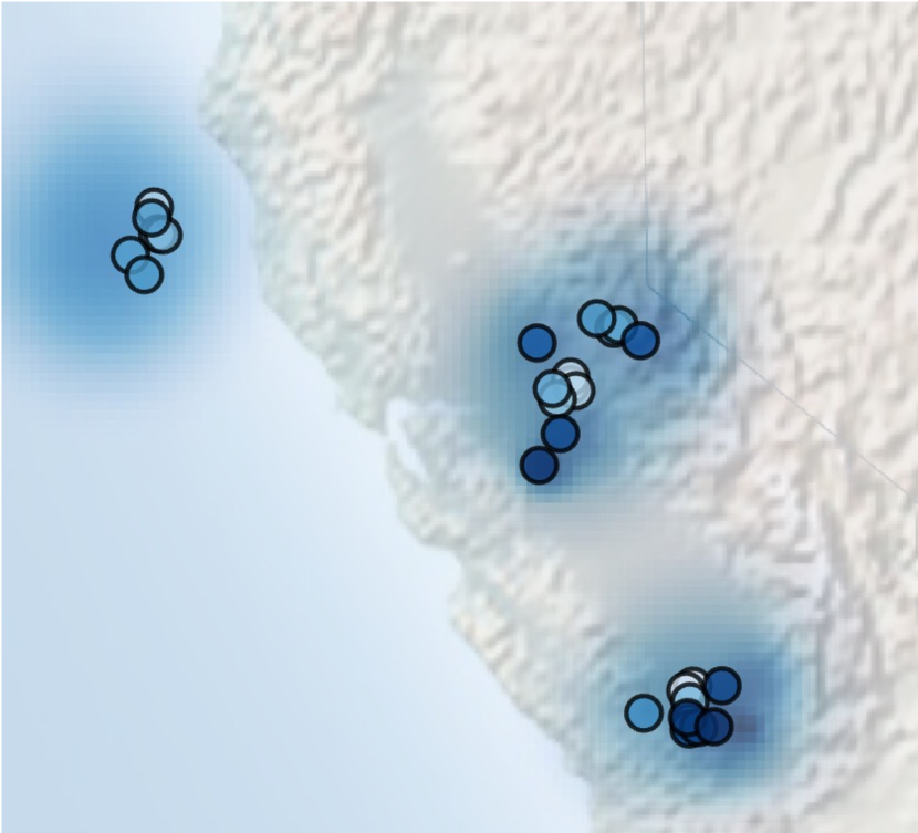
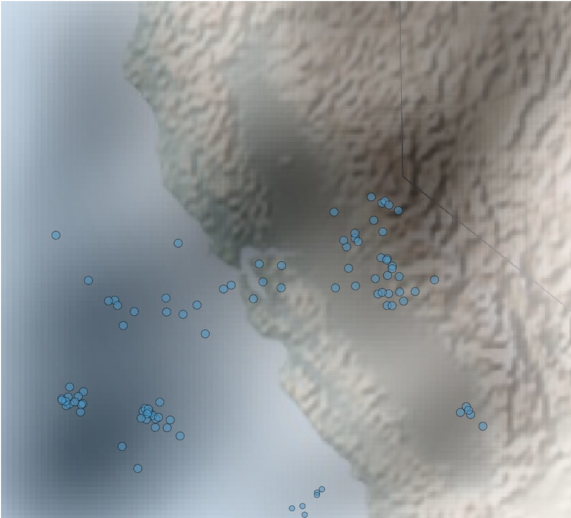
(c) ETAS

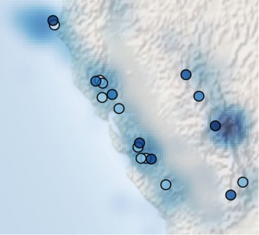
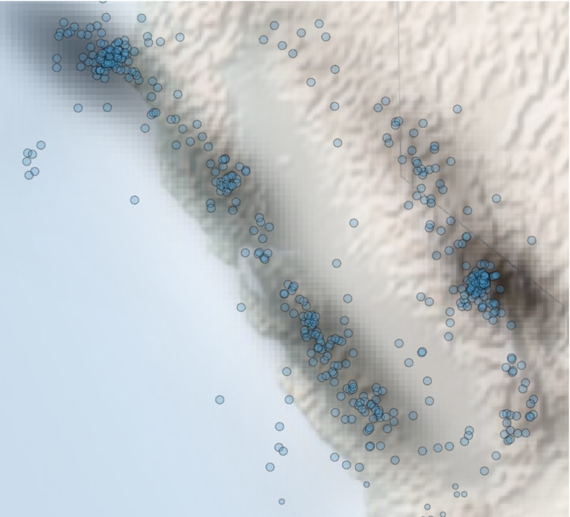
(d) CEG

Figure 5: Comparison between real and generated earthquake sequence. The first row displays a single sequence, either real or generated, with the color depth of the dots reflecting the occurrence time of each event. Darker colors represent more recent events. The shaded blue areas represent the estimated conditional PDFs. The second row shows 1,000 real or generated events, where the shaded area with grey color indicates the event density estimated by KDE, which can be interpreted as the “background rate” of the events.

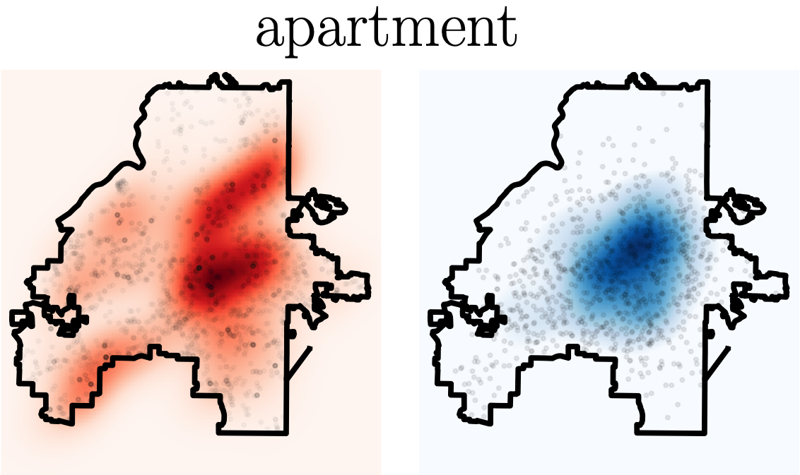
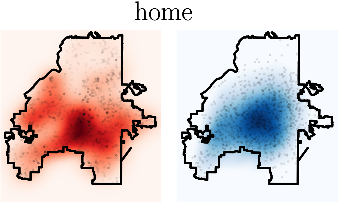
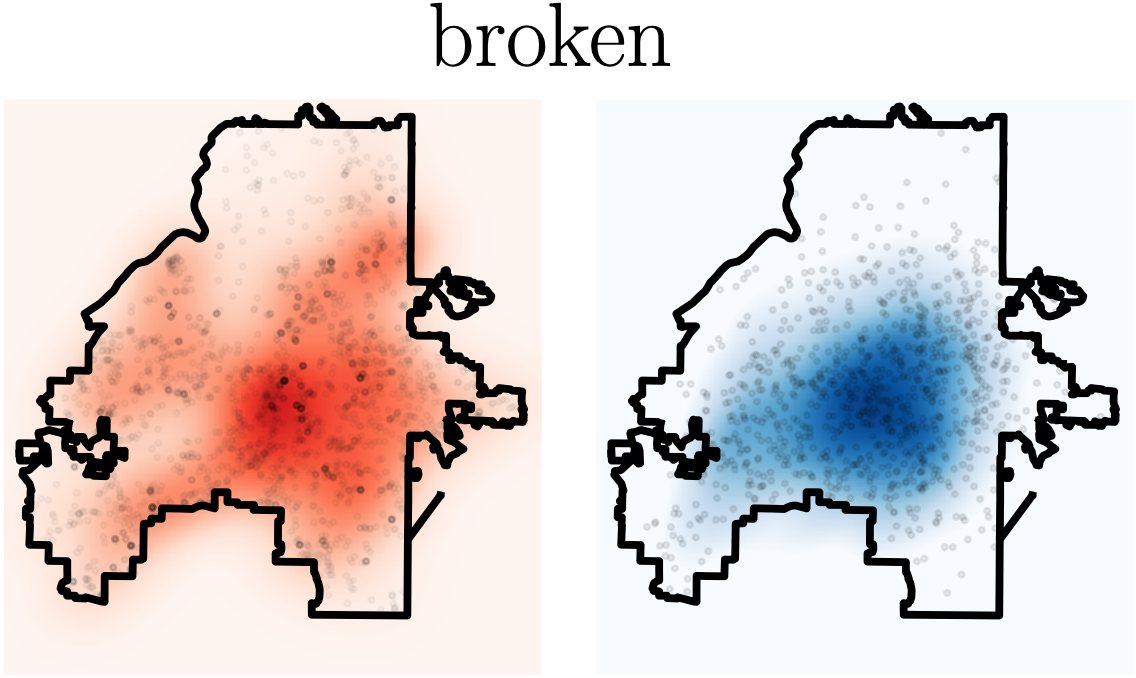
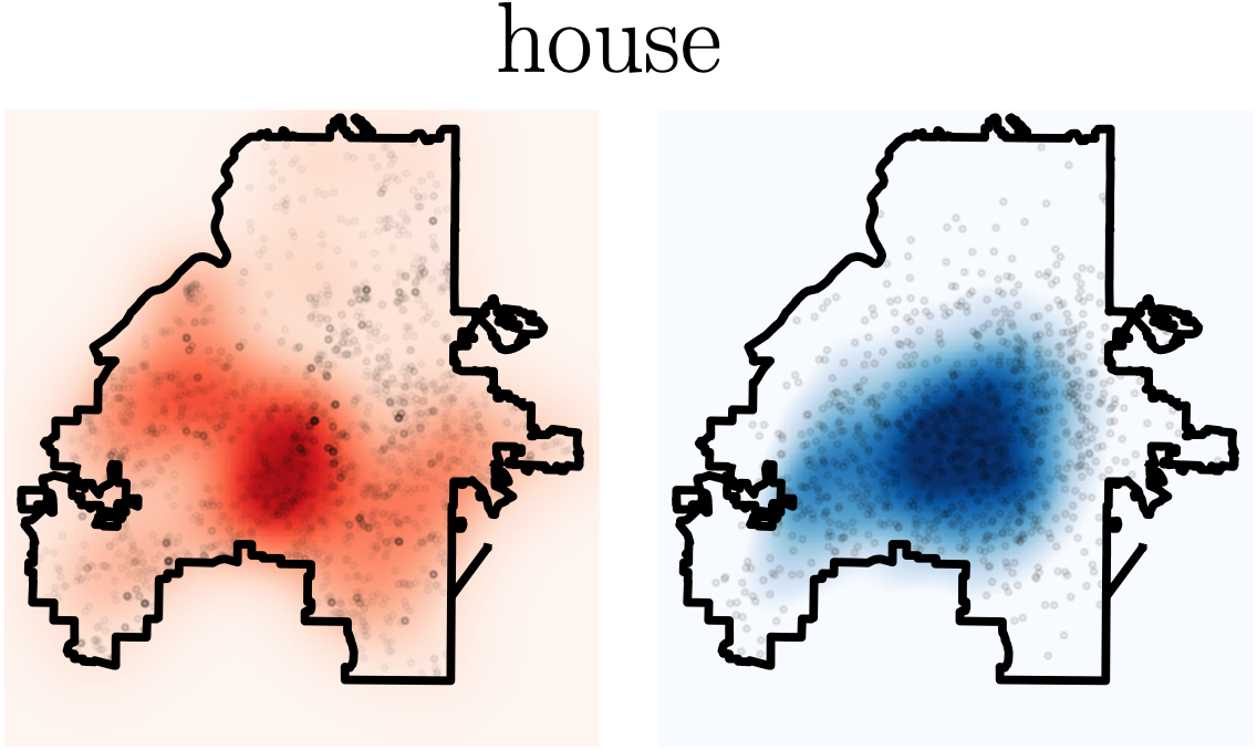
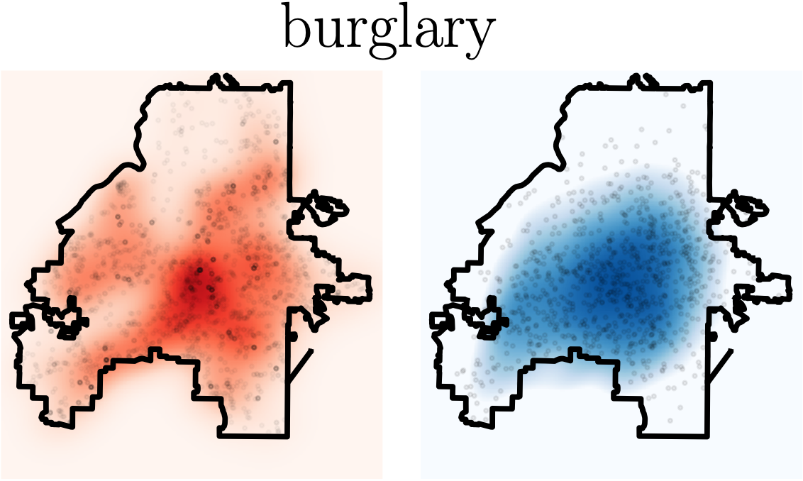
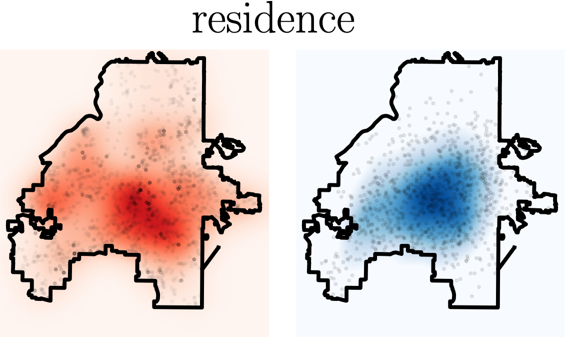
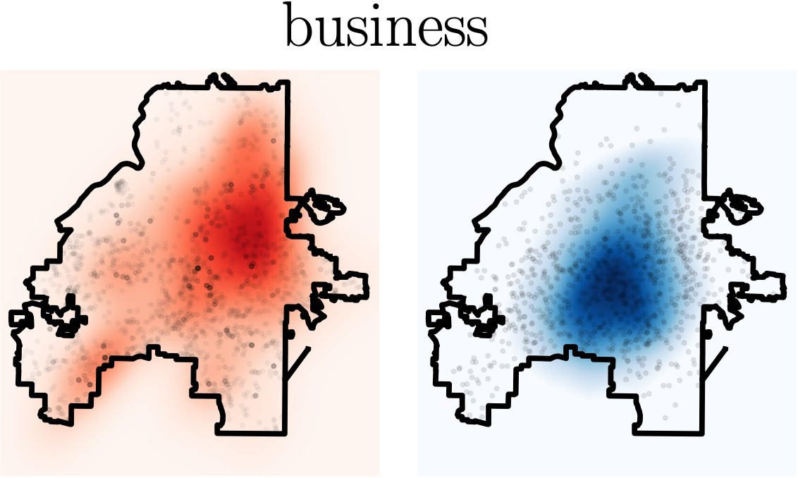
Figure 6: The spatial distributions of the TF-IDF values of 10 crime-related keywords. The heatmap in red and blue represent distributions of TF-IDF value of the keywords in the true and generated events, respectively. The black dots pinpoint the locations of the corresponding events.

Atlanta crime reports with textual description.

We further assess our method using 911-calls-for-service data in Atlanta. The proprietary data set contains 4644 burglary incidents from 2016 to 2017, detailing the time, location, and a comprehensive textual description of each incident. Each textual description was transformed into a TF-IDF vector [1], from which the top 10 keywords with the most significant TF-IDF values were selected. The location combined with the corresponding 10-dimensional TF-IDF vector is regarded as the mark of the incident. We first fit the CEG and DNSK using the preprocessed data, subsequently generate crime event sequences, and then compare them with the real data.

Figure 6 visualizes the spatial distributions of the true and the generated TF-IDF value of each keyword, respectively, signifying the heterogeneous crime patterns across the city. As we can observe, our model is capable of capturing such spatial heterogeneity for different keywords and simulating crime incidents that follow the underlying spatio-temporal-textual dynamics existing in criminological modus operandi [54]. Meanwhile, quantitative measurements for the generated event time sequences are reported in Table 2, showing the capability of our model to learn and reproduce the temporal properties of the original crime reports. Note that our model is able to simultaneously capture the data dynamics in time, location, and mark space, despite the dimensionality difference in various modalities.

4 Discussions

In this paper, we introduce a novel framework for high-dimensional marked temporal point processes for generating high-quality event series, which offers a highly adaptable and efficient solution for modeling and generating multi-dimensional event data. The proposed framework uses a conditional denoising diffusion model as the conditional event generator to explore the intricate multi-dimensional event space and generate subsequent events based on prior observations with exceptional efficiency. The empirical evaluation demonstrates the superior performance of our model in capturing complex data distribution and generating high-quality samples against state-of-the-art methods, and its flexibility of being adapting to different real-world scenarios. Finally, several promising areas for future research based on our proposed method can be foreseen. One such area involves the incorporation of more advanced generative models, thereby further facilitating the generation of high-dimensional marks. Another possibility involves the exploration of multi-modal data generation with timestamps. Moreover, the framework holds the potential to be adapted into a decision-making tool for addressing sequential decision problems within the realm of reinforcement learning.

Appendix A Derivation of the conditional probability of point processes

The conditional probability of point processes can be derived from the conditional intensity (1). Suppose we are interested in the conditional probability of events at a given point $x\in\mathcal{X}$, and we assume that there are $i$ events that happen before $t(x)$. Let $\Omega(x)$ be a small neighborhood containing $x$. According to (1), we can rewrite $\lambda(x|\mathcal{H}_{t(x)})$ as following:

$$\lambda(x|\mathcal{H}_{t(x)}) =\mathbb{E}\left(d\mathbb{N}(x)|\mathcal{H}_{t(x)}\right)/dx=\mathbb{P}\{x_{i+1}\in\Omega(x)|\mathcal{H}_{t(x)}\}/dx$$

$$=\mathbb{P}\{x_{i+1}\in\Omega(x)|\mathcal{H}_{t_{i+1}}\cup\{t_{i+1}\geq t(x)\}\}/dx$$

$$=\frac{\mathbb{P}\{x_{i+1}\in\Omega(x),t_{i+1}\geq t(x)|\mathcal{H}_{t_{i+1}}\}/dx}{\mathbb{P}\{t_{i+1}\geq t(x)|\mathcal{H}_{t_{i+1}}\}}.$$

Here $\mathcal{H}_{t_{i+1}}=\{x_{1},\dots,x_{i}\}$ represents the history up to $i$-th events. If we let $F(t(x)|\mathcal{H}_{t(x)})=\mathbb{P}(t_{i+1}<t(x)|\mathcal{H}_{t_{i+1}})$ be the conditional cumulative probability, and $f(x|\mathcal{H}_{t(x)})\triangleq f(x_{i+1}\in\Omega(x)|\mathcal{H}_{t_{i+1}})$ be the conditional probability density of the next event happening in $\Omega(x)$. Then the conditional intensity can be equivalently expressed as

$$\lambda(x|\mathcal{H}_{t(x)})=\frac{f(x|\mathcal{H}_{t(x)})}{1-F(t(x)|\mathcal{H}_{t(x)})}.$$

We multiply the differential $dx=dtdm$ on both sides of the equation and integral over the mark space $\mathcal{M}$:

$$dt\cdot\int_{\mathcal{M}}\lambda(x|\mathcal{H}_{t(x)})dm =\frac{dt\cdot\int_{\mathcal{M}}f(x|\mathcal{H}_{t(x)})dm}{1-F(t(x)|\mathcal{H}_{t(x)})}$$

$$=\frac{dF(t(x)|\mathcal{H}_{t(x)})}{1-F(t(x)|\mathcal{H}_{t(x)})}$$

$$=-d\log{(1-F(t(x)|\mathcal{H}_{t(x)}))}.$$

Hence, integrating over $t$ on $[t_{i},t(x))$ leads to the fact that

$$F(t(x)|\mathcal{H}_{t(x)}) =1-\exp\left(-\int_{t_{i}}^{t(x)}\int_{\mathcal{M}}\lambda(x|\mathcal{H}_{t(x)})dmdt\right)$$

$$=1-\exp\left(-\int_{[t_{i},t(x))\times\mathcal{M}}\lambda(x|\mathcal{H}_{t(x)})dx\right)$$

because $F(t_{i})=0$. Then we have

$$f(x|\mathcal{H}_{t(x)})=\lambda(x|\mathcal{H}_{t(x)})\cdot\exp\left(-\int_{[t_{i},t(x))\times\mathcal{M}}\lambda(x|\mathcal{H}_{t(x)})dx\right),$$

which corresponds to (2).

The log-likelihood of one observed event series in (3) is derived, by the chain rule, as

$$\ell(x_{1},\dots,x_{N_{T}}) =\log f(x_{1},\dots,x_{N_{T}})=\log\prod_{i=1}^{N_{T}}f(x_{i}|\mathcal{H}_{t_{i}})$$

$$=\int_{\mathcal{X}}\log f(x|\mathcal{H}_{t(x)})d\mathbb{N}(x)$$

$$=\int_{\mathcal{X}}\log\lambda(x|\mathcal{H}_{t(x)})d\mathbb{N}(x)-\int_{\mathcal{X}}\lambda(x|\mathcal{H}_{t(x)})dx.$$

The log-likelihood of $K$ observed event sequences in (5) can be conveniently obtained with the counting measure $\mathbb{N}$ replaced by the counting measure $\mathbb{N}_{k}$ for the $k$-th sequence.

Figure A1: A comparison between the vanilla KDE and the KDE with boundary correction. The grey shaded area indicates the true density function, which is defined on the bounded region $[0,+\infty)$. The blue dashed line and red line show the estimated density function by the vanilla KDE and the KDE with reflection, respectively.

(a) Vanilla KDE

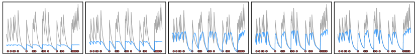
(b) KDE using self-tuned kernel

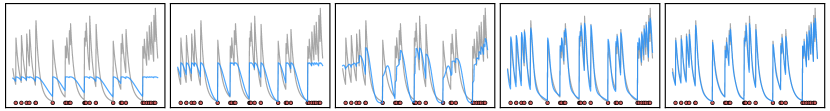
(c) KDE using self-tuned kernel with boundary correction

Figure A2: The evolution of the estimated conditional PDF $f(t|\mathcal{H}_{t})$ of an event sequence during training is displayed from left to right. Each row represents the model CEG+KDE trained with different variants of KDE. Each panel within the same row represents the estimated conditional PDF at intervals of 10 training epochs.

Appendix B Non-parametric learning using Kernel Density Estimation

This section presents a non-parametric learning strategy for estimating the conditional PDF in (5) using generated samples through kernel density estimation (KDE). Specifically, given the training data $x$ and the history embedding $\bm{h}$, we can first generate a set of samples $\{\widetilde{x}^{(l)}\}_{l=1}^{L}$, using the conditional event generator $g_{\theta}(\cdot,\bm{h})$. Then the conditional PDF of the event $x$ can be estimated by,

$$f_{\theta}(x|\bm{h})\approx\frac{1}{L}\sum_{l=1}^{L}\kappa_{\sigma}(x-\widetilde{x}^{(l)}),$$ (B1)

where $\kappa_{\sigma}$ is a kernel function with a bandwidth $\sigma$. The complete model log-likelihood can be thus estimated by generating samples at each observed event given the corresponding history.

We note two main challenges in estimating the conditional PDF $f(x|\bm{h})$ using kernel density estimation (KDE): (i) The distribution density of events can vary from location to location in the event space and may also change significantly over the training iterations. Consequently, using a single bandwidth for estimation would either oversmooth the conditional PDF or introduce excessive noise in areas with sparse events. (2) The support of the next event’s time is $[0,+\infty)$, and the time interval for the next event to come can cluster in a small neighborhood of $0$, which will lead to a significant boundary bias.

  Input: Training set $X$ with $K$ sequences: $X=\{x_{i}^{(k)}\}_{i=1,\dots,\mathbb{N}_{k}(\mathcal{X}),\ k=1,\dots,K}$, learning epoch $E$, learning rate $\gamma$, mini-batch size $M$.  

  Initialization: model parameters $\theta$, $e=0$ 

  while $e<E$ do

     for each sampled batch $\widehat{X}^{M}$ with size $M$ do

        1. Draw samples $z$ from noise distribution $\mathcal{N}(0,1)$;

        2. Feed $z$ into the generator $g$ to obtain sampled events $\widetilde{x}$;

        3. Estimate conditional PDF using KDE (B1) and log-likelihood $\ell$ (3), given data $\widehat{X}^{M}$, samples $\widetilde{x}$ and the model;

        4. $\theta\leftarrow\theta+\gamma\partial\ell/\partial\theta$;

     end for

     $e\leftarrow e+1$;

  end while

  return $\theta$  

Algorithm 3 Non-parametric learning for CEG

Implementation details

To overcome the above challenges, we adopt the self-tuned kernel [5, 24] with boundary correction [15]:

1. We first choose the bandwidth adaptively, where the bandwidth $\sigma$ tends to be small for those samples falling into event clusters and to be large for those isolated samples. We dynamically determine the value of $\sigma$ for each sample $\widetilde{x}$ by computing the $k$-nearest neighbor ($k$NN) distance among other generated samples.

2. We correct the boundary bias of KDE by reflecting the data points against the boundary $0$ in the time domain. Specifically, the kernel with reflection is defined as follows:

   $$\kappa(x-\widetilde{x})=\upsilon^{*}(\Delta t-\Delta\widetilde{t})\cdot\upsilon(m-\widetilde{m}),$$

   where $\upsilon$ is an arbitrary kernel and $\upsilon^{*}(x-\widetilde{x})=\upsilon(x-\widetilde{x})+\upsilon(-x-\widetilde{x})$ is the same kernel with reflection boundary. This allows for a more accurate estimation of the density near the boundary of the time domain without impacting the estimation elsewhere, as shown in Figure A1.

Figure A2 compares the learned conditional PDF using three KDE methods on the same synthetic data set generated by a self-exciting Hawkes process. The results show that the estimation using the self-tuned kernel with boundary correction shown in (c) significantly outperforms two ablation models in (a) and (b). We also summarize the learning algorithm in Algorithm 3.

Appendix C Variational learning

Variational method is another widely-adopted approach for learning a wide spectrum of generative models. Examples of such models include variational autoencoders [19, 20] and diffusion models [13, 16, 39]. We follow the idea of conditional variational autoencoder (CVAE) [40] and approximate the log conditional PDF using its evidence lower bound (ELBO):

$$\log f_{\theta}(x|\bm{h}) \geq-D_{\text{KL}}(q(z|x,\bm{h})||p_{\theta}(z|\bm{h}))+\mathbb{E}_{q(z|x,\bm{h})}\left[\log p_{\theta}(x|z,\bm{h})\right],$$ (C2)

where $q$ is a variational approximation of the posterior distribution over the random noise given observed event $x$ and its history summarized by $\bm{h}$. The first term on the right-hand side is the Kullback–Leibler (KL) divergence of the approximate posterior $q(\cdot|x,\bm{h})$ from the exact posterior $p_{\theta}(\cdot|\bm{h}))$. The second term is the log-likelihood of the latent data-generating process.

The derivation of the ELBO approximation for the conditional PDF in (C2) proceeds as follows. The conditional PDF of event $x$ given the history can be re-written as:

$$\log f_{\theta}(x|\bm{h})=\log\int p_{\theta}(x,z|\bm{h})dz,$$

where $z$ is a latent random variable. This integral has no closed form and can usually be estimated by Monte Carlo integration with importance sampling, i.e.,

$$\int p_{\theta}(x,z|\bm{h})dz=\mathbb{E}_{z\sim q(\cdot|x,\bm{h})}\left[\frac{p_{\theta}(x,z|\bm{h})}{q(z|x,\bm{h})}\right].$$

Here $q(z|x,\bm{h})$ is the proposed variational distribution, where we can draw sample $z$ from this distribution given $x$ and $\bm{h}$. Therefore, by Jensen’s inequality, we can find the evidence lower bound (ELBO) of the conditional PDF:

$$\log f_{\theta}(x|\bm{h}) =\log\mathbb{E}_{z\sim q(\cdot|x,\bm{h})}\left[\frac{p_{\theta}(x,z|\bm{h})}{q(z|x,\bm{h})}\right]\geq\mathbb{E}_{z\sim q(\cdot|x,\bm{h})}\left[\log\frac{p_{\theta}(x,z|\bm{h})}{q(z|x,\bm{h})}\right].$$

Using Bayes rule, the ELBO can be equivalently expressed as:

$$\mathbb{E}_{z\sim q(\cdot|x,\bm{h})}\left[\log\frac{p_{\theta}(x,z|\bm{h})}{q(z|x,\bm{h})}\right]=\leavevmode\nobreak\ \mathbb{E}_{z\sim q(\cdot|x,\bm{h})}\left[\log\frac{p_{\theta}(x|z,\bm{h})p_{\theta}(z|\bm{h})}{q(z|x,\bm{h})}\right]$$

$$=\mathbb{E}_{z\sim q(\cdot|x,\bm{h})}\left[\log\frac{p_{\theta}(z|\bm{h})}{q(z|x,\bm{h})}\right]+\mathbb{E}_{z\sim q(\cdot|x,\bm{h})}\left[\log p_{\theta}(x|z,\bm{h})\right]$$

$$=-D_{\text{KL}}(q(z|x,\bm{h})||p_{\theta}(z|\bm{h}))+\mathbb{E}_{z\sim q(\cdot|x,\bm{h})}\left[\log p_{\theta}(x|z,\bm{h})\right].$$

Implementation details

In practice of the variational learning, we introduce two additional functions in the conditional event generator, encoder net $g_{\text{encode}}(\epsilon,x,\bm{h})$ and prior net $g_{\text{prior}}(\epsilon,\bm{h})$, respectively, to represent $q(z|x,\bm{h})$ and $p_{\theta}(z|\bm{h})$ as transformations of another random variable $\epsilon\sim\mathcal{N}(0,I)$ using reparametrization trick [39]. Both $q(z|x,\bm{h})$ and $p_{\theta}(z|\bm{h})$ are often modeled as Gaussian distributions, which allows us to compute the KL divergence of Gaussians with a closed-form expression. The log-likelihood of the second term can be implemented as the reconstruction loss and calculated using generated samples.

We parameterize both $p_{\theta}(z|\bm{h})$ and $q(z|x,\bm{h})$ using fully-connected neural networks with one hidden layer, denoted by $g_{\text{prior}}$ and $g_{\text{encode}}$, respectively. The prior of the latent variable is modulated by the input $\bm{h}$ in our formulation; however, the constraint can be easily relaxed to make the latent variables statistically independent of input variables, i.e., $p_{\theta}(z|\bm{h})=p_{\theta}(z)$ [18, 40]. For the approximate posterior $q(z|x,\bm{h})$, a common choice is a simple factorized Gaussian encoder, which can be represented as:

$$q(z|x,\bm{h})=\mathcal{N}(z;\mu,\text{diag}(\Sigma)),$$

or

$$q(z|x,\bm{h})=\prod_{j=1}^{r}q(z_{j}|x,\bm{h})=\prod_{j=1}^{r}\mathcal{N}(z_{j};\mu_{j},\sigma_{j}^{2}).$$

The Gaussian parameters $\mu=(\mu_{j})_{j=1,\dots,r}$ and $\text{diag}(\Sigma)=(\sigma_{j}^{2})_{j=1,\dots,r}$ are the output of an encoder network $\phi$ and the latent variable $z$ can be obtained using reparametrization trick:

$$(\mu,\log\text{diag}(\Sigma))= \leavevmode\nobreak\ \phi(x,\bm{h}),$$

$$z= \leavevmode\nobreak\ \mu+\text{diag}(\Sigma)\odot\epsilon,$$

where $\epsilon\sim\mathcal{N}(0,I)$ is another random variable and $\odot$ is the element-wise product. For simplicity in presentation, we denote such a factorized Gaussian encoder as $g_{\text{encode}}(\epsilon,x,\bm{h})$ that maps an event $x$, its history $\bm{h}$, and a random noise vector $\epsilon$ to a sample $z$ from the approximate posterior for that event $x$.

  Input: Training set $X$ with $K$ sequences: $X=\{x_{i}^{(k)}\}_{i=1,\dots,\mathbb{N}_{k}(\mathcal{X}),\ k=1,\dots,K}$, learning epoch $E$, learning rate $\gamma$, mini-batch size $M$.  

  Initialization: model parameters $\theta$, $e=0$ 

  while $e<E$ do

     for each sampled batch $\widehat{X}^{M}$ with size $M$ do

        1. Draw samples $\epsilon$ from noise distribution $\mathcal{N}(0,1)$;

        2. Compute $z$ using reparametrization trick, given data $\widehat{X}^{M}$, noise $\epsilon$, $g_{\text{prior}}$, and $g_{\text{encode}}$;

        3. Compute ELBO (C2) and log-likelihood $\ell$ (3) based on $z$ and data $\widehat{X}^{M}$;

        4. $\theta\leftarrow\theta-\gamma\partial\ell/\partial\theta$;

     end for

     $e\leftarrow e+1$;

  end while

  return $\theta$  

Algorithm 4 Variational learning for CEG using stochastic gradient descent

In (C2), the first term is the KL divergence of the approximate posterior from the prior, which acts as a regularizer, while the second term is an expected negative reconstruction error. They can be calculated as follows: (1) Because both $q(z|x,\bm{h})$ and $p_{\theta}(z|\bm{h})$ are modeled as Gaussian distributions, the KL divergence can be computed using a closed-form expression. (2) Minimizing the negative log-likelihood $p_{\theta}(x|z,\bm{h})$ is equivalent to maximizing the cross entropy between the distribution of an observed event $x$ and the reconstructed event $\widetilde{x}$ generated by the generative model $g$ given $z$ and the history $\bm{h}$. The learning algorithm has been summarized in Algorithm 4.

Appendix D Derivation and implementation details of conditional denoising diffusion model

  Input: Training set $X$ with $K$ sequences: $X=\{x_{i}^{(k)}\}_{i=1,\dots,\mathbb{N}_{k}(\mathcal{X}),\ k=1,\dots,K}$, learning epoch $E$, learning rate $\gamma$, mini-batch size $M$.  

  Initialization: model parameters $\theta$, $e=0$ 

  while $e<E$ do

     for each sampled batch $\widehat{X}^{M}$ with size $M$ do

        1. Draw samples $(x,\bm{h})$;

        2. $\bm{h}\leftarrow\varnothing$ with probability $p_{\text{uncond}}$, where $p_{\text{uncond}}=0.1$ is a pre-chosen probability of unconditional training;

        3. $k\sim\text{Unif}(1,K),\epsilon\sim\mathcal{N}(0,I)$;

        4. Compute $\ell=\|\epsilon-\epsilon_{\theta}(\sqrt{\bar{\alpha}_{k}}x+\sqrt{1-\bar{\alpha}_{k}}\epsilon,\bm{h},k)\|^{2}$

        5. $\theta\leftarrow\theta-\gamma\partial\ell/\partial\theta$;

     end for

     $e\leftarrow e+1$;

  end while

  return $\theta$  

Algorithm 5 Training of CDDM with classifier-free guidance

In denoising diffusion models, the forward process is fixed to a Markov chain to characterize the variational distribution of latent variables:

$$q(z_{1:K}|x,\bm{h})\coloneqq\prod_{k=1}^{K}q(z_{k}|z_{k-1},\bm{h}),\quad q(z_{k}|z_{k-1},\bm{h})\coloneqq\mathcal{N}(\sqrt{1-\beta_{k}}z_{k-1},\beta_{k}I).$$

Here, we define $z_{0}\coloneqq x$. The forward process gradually adds noise to the data, and the final latent variable $z_{K}$ has the noise distribution of $\mathcal{N}(0,I)$. The variance schedule $\{\beta_{k}\}_{k=1}^{K}$ can be learned by reparameterization [19] or held constant as hyperparameters [13]. A reverse process inverts the transformation from the noise distribution with learned Gaussian transitions:

$$p_{\theta}(x,z_{1:K}|\bm{h})\coloneqq p(z_{K})\prod_{k=1}^{K}p_{\theta}(z_{k-1}|z_{k},\bm{h}),\quad p_{\theta}(z_{k-1}|z_{k},\bm{h})\coloneqq\mathcal{N}(\mu_{\theta}(z_{k},k),\Sigma_{\theta}(z_{k},k)),$$

where the mean $\mu_{\theta}$ is represented by a neural network and the covariance $\Sigma_{\theta}$ is set to be $\beta_{k}I$. The mean function $\mu_{\theta}$ can be trained by maximizing the variational bound on the log-likelihood of the data $x$:

$$\mathbb{E}[\log f_{\theta}(x|\bm{h})]\geq\mathbb{E}_{q}\left[\log p(z_{K})+\sum_{k\geq 1}\log\frac{p_{\theta}(z_{k-1}|z_{k},\bm{h})}{q(z_{k}|z_{k-1},\bm{h})}\right].$$

To optimize the above objective, we note the property of the forward process that allows the closed-form distribution of $z_{k}$ at an arbitrary step $k$ given the data $x$: denoting $\alpha_{k}\coloneqq 1-\beta_{k}$ and $\bar{\alpha}_{k}\coloneqq\prod_{r=1}^{k}\alpha_{r}$, we have $q(z_{k}|x,\bm{h})=\mathcal{N}(\sqrt{\bar{\alpha}_{k}}x,(1-\bar{\alpha}_{k})I)$. The variational bound can be therefore expressed by the KL divergence between a series of Gaussian distributions of $z_{1:K}$ and $x$, leading to the training objective of $\mathbb{E}_{q}\left[\sum_{k>1}\frac{1}{2\beta_{k}}\|\tilde{\mu}_{k}(z_{k},x)-\mu_{\theta}(z_{k},k)\|^{2}\right]+C$. Given the closed-form distribution of $z_{k}$ given $x$, we can re-parametrize $z_{k}=\sqrt{\bar{\alpha}_{k}}x+\sqrt{1-\bar{\alpha}_{k}}\epsilon$ with $\epsilon\sim\mathcal{N}(0,I)$. The model is trained on the final variant of the variational bound:

$$\mathbb{E}_{k,x,\epsilon}\left[\|\epsilon-\epsilon_{\theta}(\sqrt{\bar{\alpha}_{k}}x+\sqrt{1-\bar{\alpha}_{k}}\epsilon,\bm{h},k)\|^{2}\right].$$

Implementation details

We adopt the classifire-free diffusion guidance [14] to train the score function $\epsilon_{\theta}$. The core idea is to simultaneously train a unconditional denoising diffusion model $\epsilon^{\prime}_{\theta}(\sqrt{\bar{\alpha}_{k}}x+\sqrt{1-\bar{\alpha}_{k}}\epsilon,k)$, which later on is used to adjust the sampling steps together with the conditional denoising model. In practice, we can use a single neural network to parameterize both $\epsilon^{\prime}_{\theta}$ and $\epsilon_{\theta}$, by simply input a null token $\varnothing$ in the place of the history embedding $\bm{h}$ for the unconditional model. Therefore, we have $\epsilon^{\prime}_{\theta}=\epsilon_{\theta}(\sqrt{\bar{\alpha}_{k}}x+\sqrt{1-\bar{\alpha}_{k}}\epsilon,\varnothing,k)$. The training details can be found in Algorithm 5, and the sampling procedure has been summarized in Algorithm 2.

Appendix E Sampling efficiency comparison

Thinning algorithms are known to be challenging and suffer from low sampling efficiency. This is because (i) these algorithms require sampling uniformly in the space $\mathcal{X}$ with the upper limit of the conditional intensity $\overline{\lambda}>\lambda(x),\leavevmode\nobreak\ \forall x$, and only a few candidate points are retained in the end. (ii) the decision of whether to reject one candidate point requires the evaluation of the conditional intensity function over the entire history, which is also stochastic. This doubly stochastic trait makes the entire thinning process particularly costly when $\mathcal{X}$ is a multi-dimensional space, since it requires a drastically large number of candidate points and numerous evaluations of the conditional intensity function.

On the contrary, our model generates samples based on the underlying conditional distribution of events learned from true data, thus every generated point will be retained. Table E1 compares the time costs for ETAS, DNSK, and CEG to generate event series of length $100$ on each data set. Particularly noteworthy is that our model requires a similar amount of time to generate different numbers of sequences. This is because CEG can generate all the sequences in parallel, leveraging the benefits of the implementation of conditional generative models.

Table E1: Computation costs for generating earthquake series and time-stamped image series of length $100$ using ETAS, DNSK and CEG.

	3D earthquake data		T-MNIST		T-CIFAR
Model	$5$ sequences	$50$ sequences	$5$ sequences	$50$ sequences	$5$ sequences	$50$ sequences
ETAS	$12.4$	$118.6$	/	/	/	/
DNSK	$20.1$	$220.4$	$87.3$	$745.6$	$274.0$	$1381.9$
CEG	$<1$	$<1$	$0.6$	$0.8$	$1.1$	$1.2$

• *Unit: second.

Appendix F Experiment details and additional results

Baselines

We compare our proposed method empirically with the following baselines:

1. Recurrent Marked Temporal Point Process (RMTPP) [8] uses an RNN to capture the nonlinear relationship between both the markers and the timings of past events. It models the conditional intensity function by

   $$\lambda(t|\mathcal{H}_{t})=\exp(\bm{v}^{\top}\bm{h}_{i}+w(t-t_{i})+b),$$

   where hidden state $\bm{h}_{i}$ of the RNN represents the event history until the nearest $i$-th event $\mathcal{H}_{t_{i}}\cup\{t_{i}\}$. The $\bm{v},w,b$ are trainable parameters. The model is learned by MLE using backpropagation through time (BPTT).

2. Neural Hawkes Process (NH) [25] extends the classical Hawkes process by memorizing the long-term effects of historical events. The conditional intensity function is given by

   $$\lambda(t|\mathcal{H}_{t})=f(\bm{w}^{\top}\bm{h}_{t}),$$

   where $\bm{h}_{t}$ is a sufficient statistic of the event history modeled by the hidden state in a continuous-time LSTM, and $f(\cdot)$ is a scaled softplus function for ensuring positive output. The weight $\mathbf{w}$ is learned jointly with the LSTM through MLE.

3. Fully Neural Network based Model (FullyNN) for General Temporal Point Processes [32] models the cumulative hazard function given the history embedding $\bm{h}_{i}$, which leads to a tractable likelihood. It uses a fully-connect neural network $Z_{i}$ with a non-negative activation function for the cumulative hazard function $\Phi(\tau|\bm{h}_{i})$ where $\tau=t-t_{i}$. The conditional intensity function is obtained by computing the derivative of the network:

   $$\lambda(t|\mathcal{H}_{t})=\frac{\partial}{\partial(\tau)}\Phi(\tau|\bm{h}_{i})=\frac{\partial}{\partial(\tau)}Z_{i}(\tau),$$

   where $Z_{i}$ is the fully-connect neural network.

4. Epidemic-type aftershock sequence (ETAS) acts as a benchmark in spatio-temporal point process modeling. Denoting each event $x:=(t,s)$, ETAS adopts a Gaussian diffusion kernel in the conditional intensity as following

   $$\lambda(t,s|\mathcal{H}_{t})=\mu+\sum_{(t_{i},s_{i})\in\mathcal{H}_{t}}k(t,t_{i},s,s_{i}),$$

   where

   $$k(t,t_{i},s,s_{i})=\frac{Ce^{-\beta(t-t_{i})}}{2\pi\sqrt{|\Sigma|}(t-t_{i})}\cdot\exp{\left\{-\frac{(s-s_{i}-a)^{\top}\Sigma^{-1}(s-s_{i}-a)}{2(t-t_{i})}\right\}}.$$

   Here $\Sigma=\text{diag}(\sigma_{x}^{2},\sigma_{y}^{2})$ is a diagonal matrix representing the covariance of the spatial correlation. Note that the diffusion kernel is stationary and only depends on the spatio-temporal distance between two events. All the parameters are learnable.

5. Deep non-stationary kernel (DNSK) [6] proposes a neural-network-based influence kernel based on kernel singular value decomposition for modeling spatio-temporal point process data. In addition, their kernel can be extended to handle high-dimensional marks:

   $$k(t_{i},t-t_{i},s_{i},s-s_{i},m_{i},m)=\sum_{q=1}^{Q}\sum_{r=1}^{R}\sum_{l=1}^{L}\alpha_{lrq}\psi_{l}(t_{i})\varphi_{l}(t-t_{i})u_{r}(s_{i})v_{r}(s-s_{i})g_{q}(m_{i})h_{q}(m).$$

   Here all the basis functions are represented by fully-connected neural networks.

Synthetic data description

  Input: Model $\lambda(\cdot)$, time horizon $T$, mark space $\mathcal{M}$, Intensity upper bound $\bar{\lambda}$.  

  Initialization: $\mathcal{H}_{T}=\emptyset,t=0,i=0$ 

  while $t<T$ do

     1. Sample $u\sim\text{Unif}(0,1)$.  

     2. $t\leftarrow t-\ln u/\bar{\lambda}$.  

     3. Sample $m\sim\text{Unif}(\mathcal{M}),D\sim\text{Unif}(0,1)$.  

     4. $\lambda=\lambda(t,m|\mathcal{H}_{T})$.  

     if $D\bar{\lambda}\leq\lambda$ then

        $i\leftarrow i+1$; $t_{i}=t,m_{i}=m$.  

        $\mathcal{H}_{T}\leftarrow\mathcal{H}_{T}\cup\{(t_{i},m_{i})\}$.  

     end if

  end while

  if $t_{i}\geq T$ then

     return $\mathcal{H}_{T}-\{(t_{i},m_{i})\}$  

  else

     return $\mathcal{H}_{T}$  

  end if

Algorithm 6 Thinning algorithm

We use the following point process models to generate the one-dimensional synthetic data sets using Algorithm 6:

1. Self-exciting Hawkes process: $\lambda(t)=\mu+\sum_{t_{i}\in\mathcal{H}_{t}}\beta e^{-\beta(t-t_{i})}$, with $\mu=0.1,\beta=0.1$.

2. Self-correcting process: $\lambda(t)=\exp{\left(\mu t-\sum_{t_{i}\in\mathcal{H}_{t}}\alpha\right)}$, with $\mu=1.0,\alpha=1.0$.

3. T-MNIST: In the MNIST series, all the digits that are greater than nine will be truncated to nine. The exponentially decaying kernel for the observation times are $k(t,t_{i})=\beta e^{-\beta(t-t_{i})},\beta=0.2$.

4. T-CIFAR: The images of bicycles and motorcycles represent outdoor exercises; the apples, pears, and oranges represent food ingestion; the computer keyboards represent study/working; and the beds represent sleeping. Before 21:00, the activity series progresses with the transition probability matrix between (exercise, food ingestion, working) being

   $$P=\begin{pmatrix}0.0&1.0&0.0\\ 0.2&0.0&0.8\\ 0.2&0.3&0.5\\ \end{pmatrix}.$$

   Starting from 21:00, the probability of sleeping increases linearly from 0 to 1 at 23:00. Each series ends with the activity of sleeping. The self-correcting process for event times is set with $\mu=0.1,\alpha=0.5$, indicating that each activity will last for a while before the student moves to the next activity (or stays in the current one).

Experimental setup

We choose our score function $\epsilon_{\theta}$ to be a fully-connected neural network with three hidden layers of width $128$ with softplus activation function. To guarantee that the generated time interval is always positive, we transforms the time dimension of the generated samples with a softplus function $\text{Softplus}(x)=\frac{1}{\beta}\log\left(1+e^{\beta x}\right)$ (The time dimensional of the training data is also transformed through the reverse of this softplus function before feeding into the model). We use an LSTM for the history encoder $\psi$. We train our model and other baselines using $90\%$ of the data and test them on the remaining $10\%$ data. To fit the model parameters, we maximize log-likelihood according to (5), and adopt Adam optimizer [17] with a learning rate of $10^{-3}$ and a batch size of 32 (event sequences).

For RMTPP, NH and FullyNN, we take the default parameters for model architectures in the original papers, with the dimension of history embedding to be $64$ for all three models, and a fully-connected neural network with two hidden layers of width $64$ for the cumulative hazard function in FullyNN. There is no hyperparameter in ETAS. All the baselines are trained using the Adam optimizer with a learning rate of $10^{-3}$ and a batch size of 32 for 100 epochs. The experiments are implemented on Google Colaboratory (Pro version) with 12GB RAM and a Tesla T4 GPU.

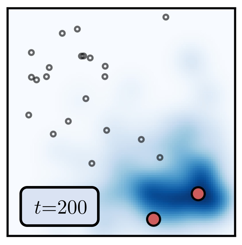
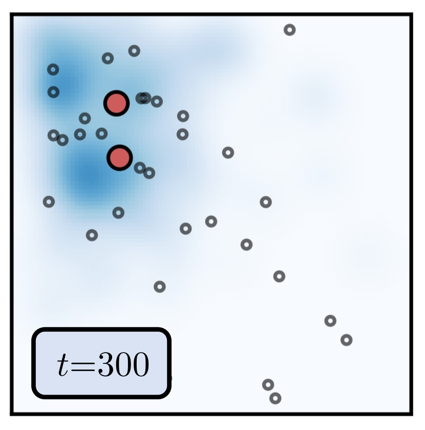
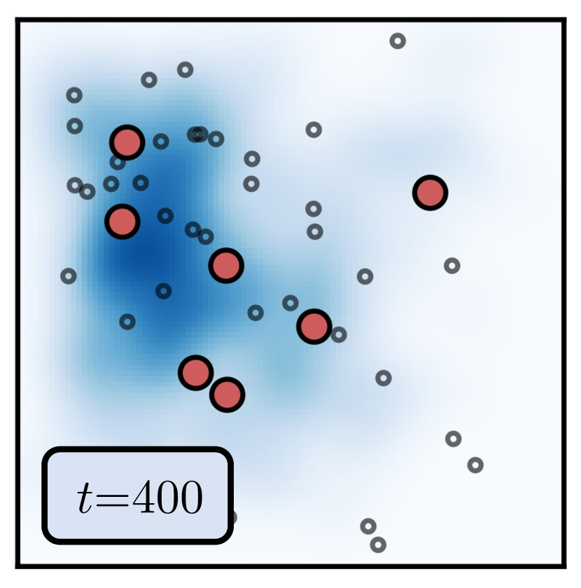
(a) Ground truth

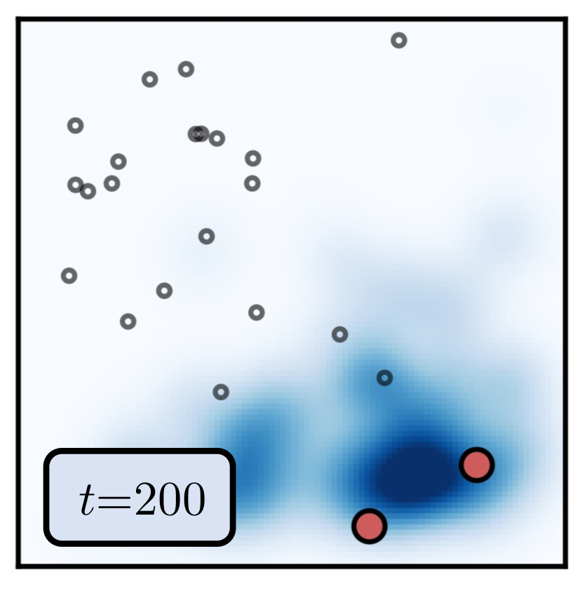
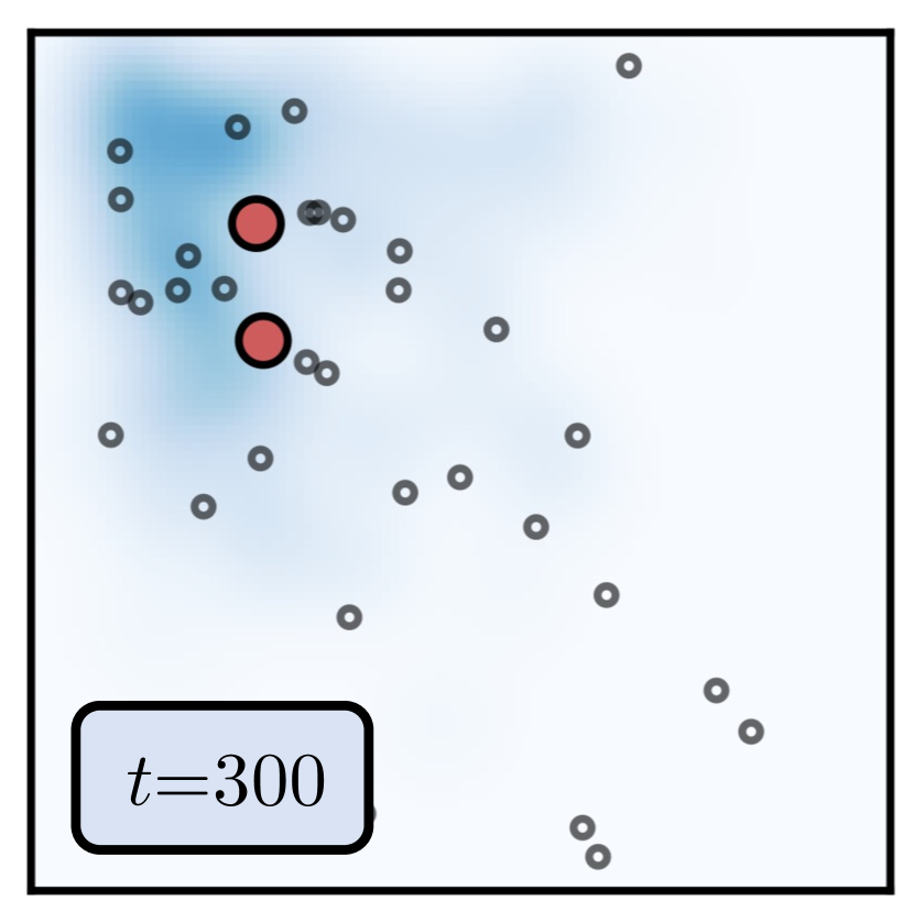
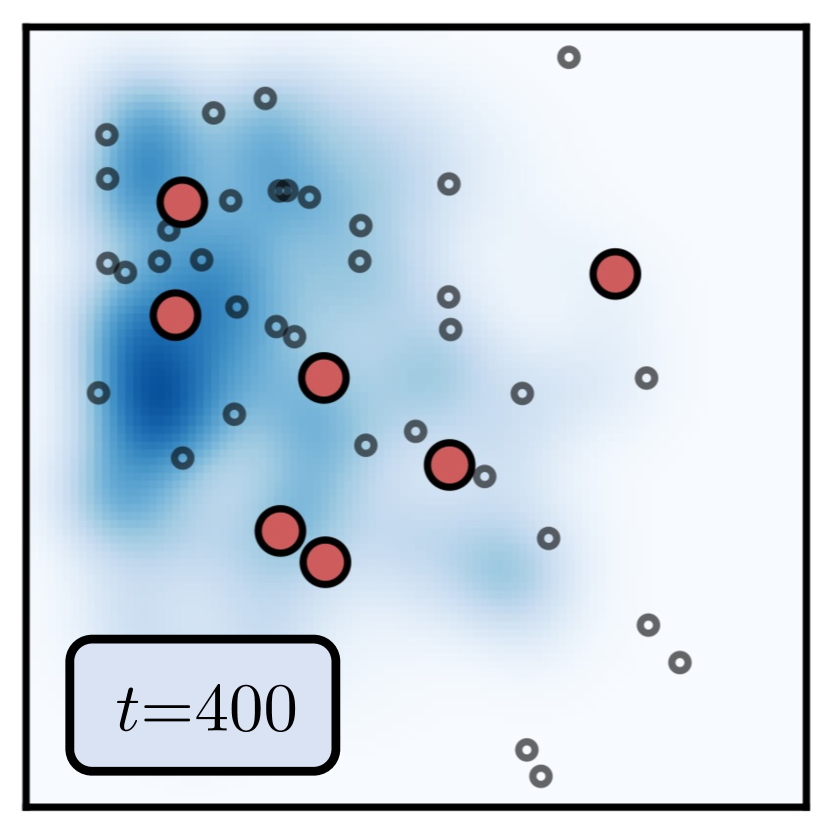
(b) CEG+CDDM

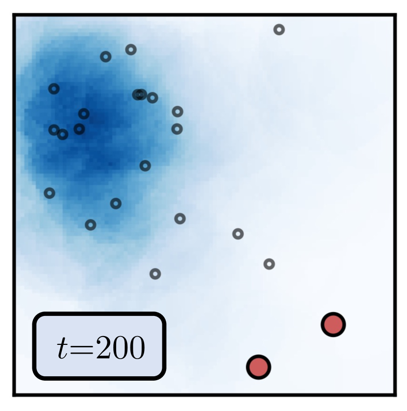
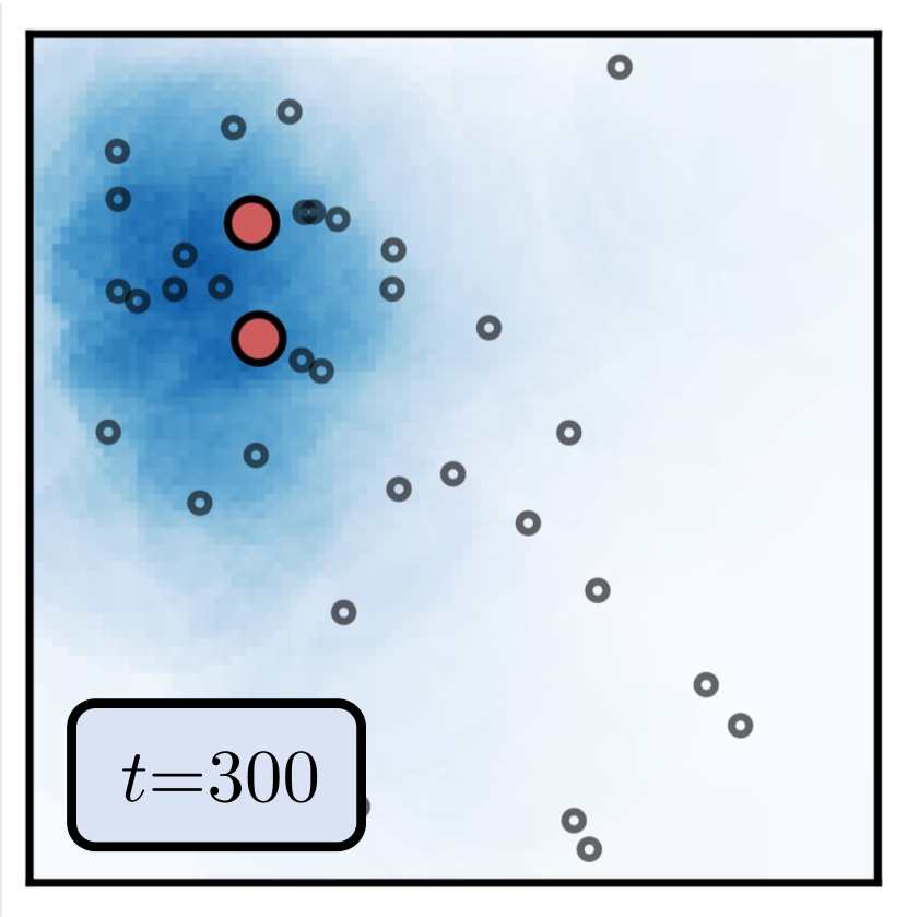
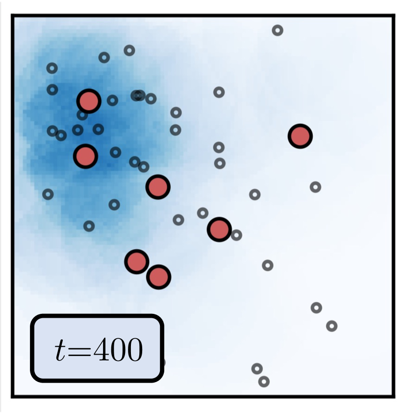
(c) DNSK

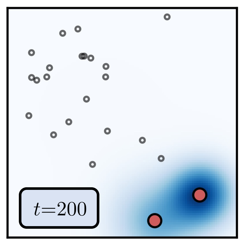
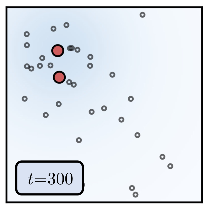
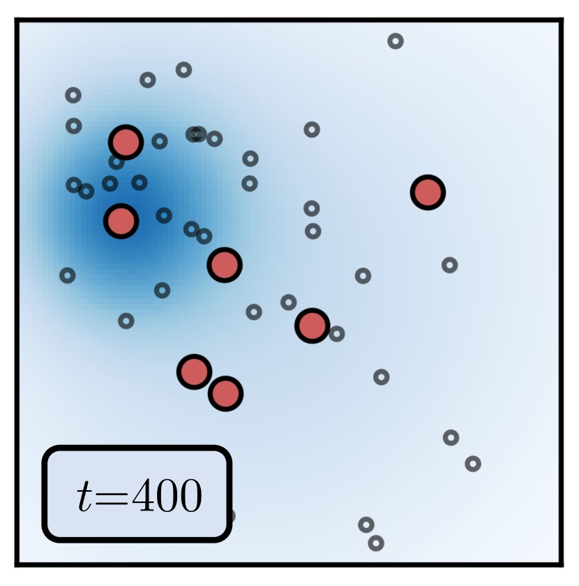
(d) ETAS

Figure F3: Snapshots of out-of-sample estimation of the conditional PDFs for a three-dimensional (time and space) synthetic event sequence, arranged in chronological order from left to right. The conditional PDFs are indicated by shaded areas, with darker shades indicating higher conditional PDF values. The red dots represent newly observed events within the most recent time period, while the circles represent historical events.

Evaluation metrics for synthesized time series

Similar to the idea of evaluating the fidelity and the diversity of the generated image samples in the image generation task, the following predictive score and the discriminative score [47] are adopted by the time-series research community:

• Predictive score: the generative model is expected to capture the conditional distributions of events over time in order to be useful. To measure this, using the generated dataset, we can train a post-hoc sequence-prediction model (usually a 2-layer LSTM) to perform one-step-ahead prediction. Then, we evaluate the trained model on the original (real) dataset in terms of the mean absolute error (MAE) of the predicted next event time. A lower predictive score indicates that the generated data better reproduces the temporal properties of the original data. This evaluation paradigm is known as train-synthesized-test-real (TSTR).

• Discriminative score: To quantitatively assess the similarity of the generated samples to the original ones, we train a post-hoc time-series classification model (usually a 2-layer LSTM) to distinguish whether the sample is real or fake. We use 80% of all the samples as training set to the classifier and evaluate it on the rest 20%. A lower classification accuracy (i.e., a lower discriminator score) means that the real and generated samples are more similar.

F.1 Additional experiment results

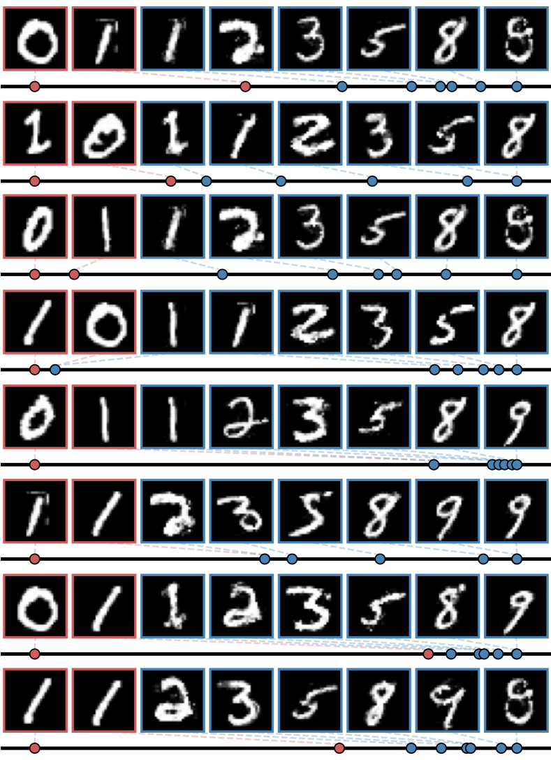
(a) Additional T-MNIST series generated by CEG

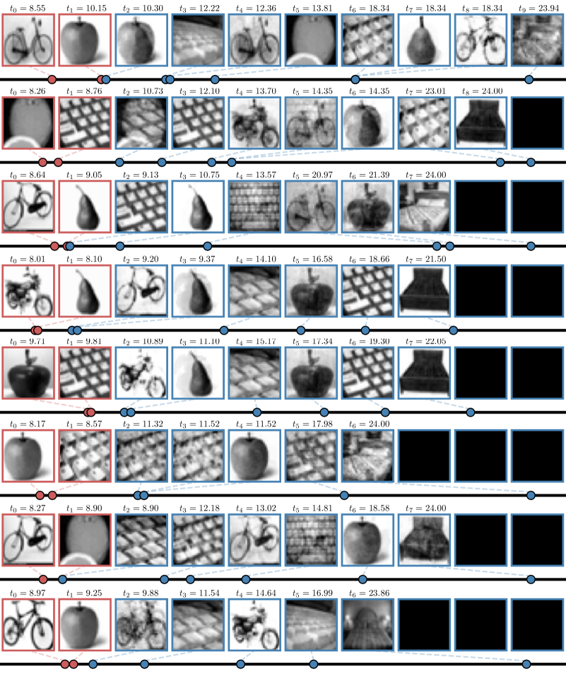
(b) Additional T-CIFAR series generated by CEG

Figure F4: Additional T-MNIST and T-CIFAR series using CEG and a neural point process baseline DNSK, with true sequences displayed on the left. Each event series is generated (blue boxes) given the first two true events (red boxes).

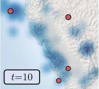
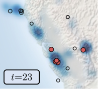
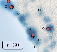
(a) CEG

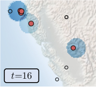
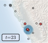
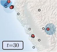
(b) DNSK

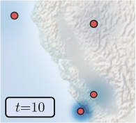
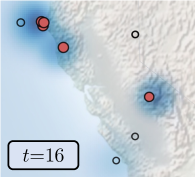
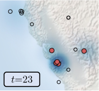
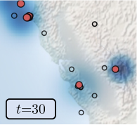
(c) ETAS

Figure F5: Estimated conditional PDFs of an actual earthquake sequence represented by shaded areas, with darker shades indicating higher conditional PDF values. Each row contains four sub-figures, arranged in chronological order from left to right, showing snapshots of the estimated conditional PDFs. The red dots represent newly observed events within the most recent time period, while the circles represent historical events.

3D synthetic data

Each row in Figure F3 displays four snapshots of estimated conditional probability density functions (PDFs) for a particular 3D testing sequence. It is apparent that our model’s estimated PDFs closely match the ground truth and accurately capture the complex spatial and temporal point patterns. Conversely, DNSK and ETAS model for estimating spatio-temporal point processes fails to capture the heterogeneous triggering effects between events, indicating limited practical representational power.

Semi-synthetic image data

More generated T-MNIST and T-CIFAR series by CEG are presented in Figure F4. As we can see, our generative point process can not only sample images that resemble the ground truth, but also recover the intricate temporal dynamics (e.g., clustering effect of self-exciting process in T-MNIST, student’s sleeping time in T-CIFAR) and high-dimensional mark dependencies.

Northern California earthquake catalog

Additional results in Figure F5 visualizes the conditional PDF estimated by CEG, DNSK, and ETAS for an actual earthquake sequence in testing set, respectively. The results indicate that our model is able to capture the heterogeneous effects among earthquakes. Particularly noteworthy is our model’s finding of a heightened probability of seismic activity along the San Andreas fault, coupled with a diminished likelihood in the basin. These results align with current understandings of the mechanics of earthquakes in Northern California. However, both DNSK and ETAS fail to extract this geographical feature from the data and suggest that observed earthquakes impact their surroundings uniformly, leading to an increased likelihood of aftershocks within a circular area centered on the location of the initial event.

References

- Aizawa, [2003] Aizawa, A. (2003). An information-theoretic perspective of tf–idf measures. Information Processing & Management, 39(1):45–65.
- Ajay et al., [2022] Ajay, A., Du, Y., Gupta, A., Tenenbaum, J., Jaakkola, T., and Agrawal, P. (2022). Is conditional generative modeling all you need for decision-making? arXiv preprint arXiv:2211.15657.
- Bond-Taylor et al., [2021] Bond-Taylor, S., Leach, A., Long, Y., and Willcocks, C. G. (2021). Deep generative modelling: A comparative review of vaes, gans, normalizing flows, energy-based and autoregressive models. IEEE transactions on pattern analysis and machine intelligence.
- Chen et al., [2020] Chen, R. T., Amos, B., and Nickel, M. (2020). Neural spatio-temporal point processes. arXiv preprint arXiv:2011.04583.
- Cheng and Wu, [2022] Cheng, X. and Wu, H.-T. (2022). Convergence of graph laplacian with knn self-tuned kernels. Information and Inference: A Journal of the IMA, 11(3):889–957.
- Dong et al., [2022] Dong, Z., Cheng, X., and Xie, Y. (2022). Spatio-temporal point processes with deep non-stationary kernels. arXiv preprint arXiv:2211.11179.
- Dong et al., [2023] Dong, Z., Zhu, S., Xie, Y., Mateu, J., and Rodríguez-Cortés, F. J. (2023). Non-stationary spatio-temporal point process modeling for high-resolution COVID-19 data. Journal of the Royal Statistical Society Series C: Applied Statistics. qlad013.
- Du et al., [2016] Du, N., Dai, H., Trivedi, R., Upadhyay, U., Gomez-Rodriguez, M., and Song, L. (2016). Recurrent marked temporal point processes: Embedding event history to vector. In Proceedings of the 22nd ACM SIGKDD international conference on knowledge discovery and data mining, pages 1555–1564.
- Goodfellow et al., [2014] Goodfellow, I., Pouget-Abadie, J., Mirza, M., Xu, B., Warde-Farley, D., Ozair, S., Courville, A., and Bengio, Y. (2014). Generative adversarial nets. In Ghahramani, Z., Welling, M., Cortes, C., Lawrence, N., and Weinberger, K., editors, Advances in Neural Information Processing Systems, volume 27. Curran Associates, Inc.
- Graves and Graves, [2012] Graves, A. and Graves, A. (2012). Long short-term memory. Supervised sequence labelling with recurrent neural networks, pages 37–45.
- Hawkes, [1971] Hawkes, A. G. (1971). Spectra of some self-exciting and mutually exciting point processes. Biometrika, 58(1):83–90.
- Heusel et al., [2017] Heusel, M., Ramsauer, H., Unterthiner, T., Nessler, B., and Hochreiter, S. (2017). Gans trained by a two time-scale update rule converge to a local nash equilibrium. Advances in neural information processing systems, 30.
- Ho et al., [2020] Ho, J., Jain, A., and Abbeel, P. (2020). Denoising diffusion probabilistic models. Advances in Neural Information Processing Systems, 33:6840–6851.
- Ho and Salimans, [2022] Ho, J. and Salimans, T. (2022). Classifier-free diffusion guidance. arXiv preprint arXiv:2207.12598.
- Jones, [1993] Jones, M. C. (1993). Simple boundary correction for kernel density estimation. Statistics and computing, 3:135–146.
- Kingma et al., [2021] Kingma, D., Salimans, T., Poole, B., and Ho, J. (2021). Variational diffusion models. Advances in neural information processing systems, 34:21696–21707.
- Kingma and Ba, [2014] Kingma, D. P. and Ba, J. (2014). Adam: A method for stochastic optimization. arXiv preprint arXiv:1412.6980.
- Kingma et al., [2014] Kingma, D. P., Mohamed, S., Jimenez Rezende, D., and Welling, M. (2014). Semi-supervised learning with deep generative models. Advances in neural information processing systems, 27.
- Kingma and Welling, [2014] Kingma, D. P. and Welling, M. (2014). Auto-Encoding Variational Bayes. In 2nd International Conference on Learning Representations, ICLR 2014, Banff, AB, Canada, April 14-16, 2014, Conference Track Proceedings.
- Kingma et al., [2019] Kingma, D. P., Welling, M., et al. (2019). An introduction to variational autoencoders. Foundations and Trends® in Machine Learning, 12(4):307–392.
- Li et al., [2020] Li, L., Yan, J., Wang, H., and Jin, Y. (2020). Anomaly detection of time series with smoothness-inducing sequential variational auto-encoder. IEEE transactions on neural networks and learning systems, 32(3):1177–1191.
- Li et al., [2018] Li, S., Xiao, S., Zhu, S., Du, N., Xie, Y., and Song, L. (2018). Learning temporal point processes via reinforcement learning. In Bengio, S., Wallach, H., Larochelle, H., Grauman, K., Cesa-Bianchi, N., and Garnett, R., editors, Advances in Neural Information Processing Systems, volume 31. Curran Associates, Inc.
- Lin et al., [2022] Lin, H., Wu, L., Zhao, G., Pai, L., and Li, S. Z. (2022). Exploring generative neural temporal point process. Transactions on Machine Learning Research.
- Mall et al., [2013] Mall, R., Langone, R., and Suykens, J. A. (2013). Self-tuned kernel spectral clustering for large scale networks. In 2013 IEEE International Conference on Big Data, pages 385–393. IEEE.
- Mei and Eisner, [2017] Mei, H. and Eisner, J. M. (2017). The neural hawkes process: A neurally self-modulating multivariate point process. Advances in neural information processing systems, 30.
- Mirza and Osindero, [2014] Mirza, M. and Osindero, S. (2014). Conditional generative adversarial nets. arXiv preprint arXiv:1411.1784.
- Mohler et al., [2011] Mohler, G. O., Short, M. B., Brantingham, P. J., Schoenberg, F. P., and Tita, G. E. (2011). Self-exciting point process modeling of crime. Journal of the American Statistical Association, 106(493):100–108.
- Northern California Earthquake Data Center. UC Berkeley Seismological Laboratory. Dataset, [2014] Northern California Earthquake Data Center. UC Berkeley Seismological Laboratory. Dataset (2014). NCEDC.
- Ogata, [1981] Ogata, Y. (1981). On lewis’ simulation method for point processes. IEEE transactions on information theory, 27(1):23–31.
- Ogata, [1998] Ogata, Y. (1998). Space-time point-process models for earthquake occurrences. Annals of the Institute of Statistical Mathematics, 50:379–402.
- Okawa et al., [2021] Okawa, M., Iwata, T., Tanaka, Y., Toda, H., Kurashima, T., and Kashima, H. (2021). Dynamic hawkes processes for discovering time-evolving communities’ states behind diffusion processes. In Proceedings of the 27th ACM SIGKDD Conference on Knowledge Discovery & Data Mining, pages 1276–1286.
- Omi et al., [2019] Omi, T., ueda, n., and Aihara, K. (2019). Fully neural network based model for general temporal point processes. In Wallach, H., Larochelle, H., Beygelzimer, A., d'Alché-Buc, F., Fox, E., and Garnett, R., editors, Advances in Neural Information Processing Systems, volume 32. Curran Associates, Inc.
- Reinhart, [2018] Reinhart, A. (2018). A review of self-exciting spatio-temporal point processes and their applications. Statistical Science, 33(3):299–318.
- Salimans et al., [2016] Salimans, T., Goodfellow, I., Zaremba, W., Cheung, V., Radford, A., and Chen, X. (2016). Improved techniques for training gans. Advances in neural information processing systems, 29.
- Sharma et al., [2019] Sharma, A., Ghosh, A., and Fiterau, M. (2019). Generative sequential stochastic model for marked point processes. In ICML Time Series Workshop.
- Shchur et al., [2020] Shchur, O., Biloš, M., and Günnemann, S. (2020). Intensity-free learning of temporal point processes. In International Conference on Learning Representations.
- Shchur et al., [2021] Shchur, O., Türkmen, A. C., Januschowski, T., and Günnemann, S. (2021). Neural temporal point processes: A review. arXiv preprint arXiv:2104.03528.
- [38] Sohl-Dickstein, J., Weiss, E., Maheswaranathan, N., and Ganguli, S. (2015a). Deep unsupervised learning using nonequilibrium thermodynamics. In International Conference on Machine Learning, pages 2256–2265. PMLR.
- [39] Sohl-Dickstein, J., Weiss, E., Maheswaranathan, N., and Ganguli, S. (2015b). Deep unsupervised learning using nonequilibrium thermodynamics. In Bach, F. and Blei, D., editors, Proceedings of the 32nd International Conference on Machine Learning, volume 37 of Proceedings of Machine Learning Research, pages 2256–2265, Lille, France. PMLR.
- Sohn et al., [2015] Sohn, K., Lee, H., and Yan, X. (2015). Learning structured output representation using deep conditional generative models. Advances in neural information processing systems, 28.
- Song and Ermon, [2019] Song, Y. and Ermon, S. (2019). Generative modeling by estimating gradients of the data distribution. Advances in neural information processing systems, 32.
- Song et al., [2020] Song, Y., Sohl-Dickstein, J., Kingma, D. P., Kumar, A., Ermon, S., and Poole, B. (2020). Score-based generative modeling through stochastic differential equations. arXiv preprint arXiv:2011.13456.
- Vaswani et al., [2017] Vaswani, A., Shazeer, N., Parmar, N., Uszkoreit, J., Jones, L., Gomez, A. N., Kaiser, Ł., and Polosukhin, I. (2017). Attention is all you need. Advances in neural information processing systems, 30.
- Wallace, [1990] Wallace, R. E. (1990). The san andreas fault system, california: An overview of the history, geology, geomorphology, geophysics, and seismology of the most well known plate-tectonic boundary in the world.
- Williams et al., [2020] Williams, A., Degleris, A., Wang, Y., and Linderman, S. (2020). Point process models for sequence detection in high-dimensional neural spike trains. Advances in neural information processing systems, 33:14350–14361.
- Xiao et al., [2018] Xiao, S., Xu, H., Yan, J., Farajtabar, M., Yang, X., Song, L., and Zha, H. (2018). Learning conditional generative models for temporal point processes. In Proceedings of the AAAI Conference on Artificial Intelligence, volume 32.
- Yoon et al., [2019] Yoon, J., Jarrett, D., and van der Schaar, M. (2019). Time-series generative adversarial networks. In Wallach, H., Larochelle, H., Beygelzimer, A., d'Alché-Buc, F., Fox, E., and Garnett, R., editors, Advances in Neural Information Processing Systems, volume 32. Curran Associates, Inc.
- Yu et al., [2019] Yu, Y., Si, X., Hu, C., and Zhang, J. (2019). A review of recurrent neural networks: Lstm cells and network architectures. Neural computation, 31(7):1235–1270.
- Yuan et al., [2023] Yuan, Y., Ding, J., Shao, C., Jin, D., and Li, Y. (2023). Spatio-temporal diffusion point processes. arXiv preprint arXiv:2305.12403.
- [50] Zhou, Z., Yang, X., Rossi, R., Zhao, H., and Yu, R. (2022a). Neural point process for learning spatiotemporal event dynamics. In Learning for Dynamics and Control Conference, pages 777–789. PMLR.
- [51] Zhou, Z., Yang, X., Rossi, R., Zhao, H., and Yu, R. (2022b). Neural point process for learning spatiotemporal event dynamics. In Firoozi, R., Mehr, N., Yel, E., Antonova, R., Bohg, J., Schwager, M., and Kochenderfer, M., editors, Proceedings of The 4th Annual Learning for Dynamics and Control Conference, volume 168 of Proceedings of Machine Learning Research, pages 777–789. PMLR.
- [52] Zhu, S., Li, S., Peng, Z., and Xie, Y. (2021a). Imitation learning of neural spatio-temporal point processes. IEEE Transactions on Knowledge and Data Engineering, 34(11):5391–5402.
- Zhu et al., [2022] Zhu, S., Wang, H., Cheng, X., and Xie, Y. (2022). Neural spectral marked point processes. In International Conference on Learning Representations.
- Zhu and Xie, [2022] Zhu, S. and Xie, Y. (2022). Spatiotemporal-textual point processes for crime linkage detection. The Annals of Applied Statistics, 16(2):1151–1170.
- Zhu et al., [2023] Zhu, S., Yuchi, H. S., Zhang, M., and Xie, Y. (2023). Sequential adversarial anomaly detection for one-class event data. INFORMS Journal on Data Science.
- [56] Zhu, S., Zhang, M., Ding, R., and Xie, Y. (2021b). Deep fourier kernel for self-attentive point processes. In Banerjee, A. and Fukumizu, K., editors, Proceedings of The 24th International Conference on Artificial Intelligence and Statistics, volume 130 of Proceedings of Machine Learning Research, pages 856–864. PMLR.
- Zuo et al., [2020] Zuo, S., Jiang, H., Li, Z., Zhao, T., and Zha, H. (2020). Transformer hawkes process. In International conference on machine learning, pages 11692–11702. PMLR.