Testing Unification and Dark Matter with Gravitational Waves

Abstract

We propose to search for a new type of gravitational wave signature relevant for particle physics models with symmetries broken at vastly different energy scales. The spectrum contains a characteristic double-peak structure consisting of a sharp peak from domain walls and a smooth bump from a first order phase transition in the early Universe. We demonstrate how such a gravitational wave signal arises in a new theory unifying baryon number and color into an SU(4) gauge group broken at the multi-TeV scale, and with lepton number promoted to an SU(2) gauge symmetry broken at the multi-EeV scale. The model contains two types of dark matter particles, explains the observed domination of matter over antimatter in the Universe, and accommodates nonzero neutrino masses. We discuss how future gravitational wave experiments, such as LISA, Big Bang Observer, DECIGO, Einstein Telescope, and Cosmic Explorer, can be utilized to look for this novel signature.

I Introduction

The Standard Model of elementary particle physics is a gauge theory based on the symmetry group

$${\rm SU}(3)_{c}\times{\rm SU}(2)_{L}\times{\rm U}(1)_{Y}\ .$$ (1)

The electroweak sector of the theory was formulated in the 1960s Glashow (1961); Higgs (1964); Englert and Brout (1964); Weinberg (1967); Salam (1968), whereas the quantum chromodynamics part was constructed in the 1970s Fritzsch et al. (1973); Gross and Wilczek (1973); Politzer (1973). Since then, the model has withstood all experimental tests, culminating in the discovery of the Higgs particle at the Large Hadron Collider in 2012 Chatrchyan et al. (2012); Aad et al. (2012). Despite this huge success, the Standard Model on its own is not complete, since it does not accommodate: $(a)$ dark matter, $(b)$ matter-antimatter asymmetry of the Universe, and $(c)$ nonzero neutrino masses.

The symmetry structure in Eq. (1) is rather complex and its origins are not understood. There is no theoretical reason to expect that this exact gauge symmetry persists all the way up to the Planck scale. Indeed, the Standard Model symmetry might be just a low-energy manifestation of a larger gauge group existing at higher energy scales, just like ${\rm U}(1)_{\rm EM}$ is a leftover symmetry from the breaking of ${\rm SU}(2)_{L}\times{\rm U}(1)_{Y}$ at the electroweak scale. Additionally, the outstanding open questions require new fields to be introduced into the theory – such new fields would most naturally be part of a gauge structure beyond that of the Standard Model.

Specifically, the evidence for the existence of dark matter has piled up over the last decades Rubin and Ford (1970); de Bernardis et al. (2000); Gavazzi et al. (2007), but the strength of its interactions with the Standard Model remains unknown, with only upper limits set by various experiments (for a review, see Feng (2010)). Although the pessimistic scenario, in which the dark matter particle is completely decoupled from the Standard Model, is a viable possibility, the hope is that the dark matter actually constitutes an integral part of a larger particle physics structure involving nonzero interactions with the known particles. In such a case, there must exist a gauge symmetry describing how the dark matter fits into the entire particle physics picture. This framework could also offer explanations for other pressing problems, such as the origin of the matter-antimatter asymmetry of the Universe or the mechanism behind neutrino masses.

In this work, we propose a new gauge extension of the Standard Model which accomplishes the above-mentioned goals, adopting elements of the models constructed in Fornal et al. (2015) and Fornal et al. (2017). This theory contains two possible GeV-scale candidates for the dark matter particle, while the observed excess of matter over antimatter is explained in an asymmetric dark matter setting, i.e., the dark matter and ordinary matter asymmetries share a common origin Nussinov (1985); Kaplan (1992); Hooper et al. (2005); Kaplan et al. (2009); Petraki and Volkas (2013); Zurek (2014). The out-of-equilibrium dynamics needed for a successful baryogenesis/leptogenesis is provided by two first order phase transitions in the early Universe. The energy scales for those phenomena are free parameters, and we consider the scenario in which both of them are high, inaccessible at the Large Hadron Collider. However, such high symmetry breaking scales make the model ideal for being probed in gravitational wave experiments.

Indeed, the much needed breakthrough in particle physics might come from the detection of primordial gravitational waves. Thus far, the Laser Interferometer Gravitational Wave Observatory (LIGO) within the LIGO/Virgo collaboration has discovered signals coming from black hole/neutron star mergers Abbott et al. (2016), however, a stochastic gravitational wave background from the early Universe is predicted by many models of physics beyond the Standard Model. Although LIGO is currently sensitive to a relatively small parameter space of such models, the reach will be considerably improved with future upgrades, as well as other planned gravitational wave experiments, such as the Laser Interferometer Space Antenna (LISA) Amaro-Seoane et al. (2017), Big Bang Observer (BBO) Crowder and Cornish (2005), DECIGO Kawamura et al. (2011), Einstein Telescope (ET) Punturo et al. (2010) and Cosmic Explorer (CE) Reitze et al. (2019). The possible sources for this stochastic gravitational wave signal are: first order phase transitions in the early Universe after inflation Kosowsky et al. (1992), inflation itself Turner (1997), and topological defects (domain walls Hiramatsu et al. (2010) and cosmic strings Vachaspati and Vilenkin (1985); Sakellariadou (1990)). In the model we propose, gravitational waves originate from annihilating domain walls and a first order phase transition.

Domain walls are topological defects which are created when a discrete symmetry is spontaneously broken Kibble (1976). They exist around boundaries of regions corresponding to different vacua. Stable domain wall configurations would lead to cosmological problems, since they would overclose the Universe. However, if the two vacua have different energy densities (this difference is called the potential bias), then domain walls become unstable and annihilate, leading to a stochastic gravitational wave background, apriori measurable today. This can be realized in many particle physics scenarios, e.g., electroweak-scale new physics Eto et al. (2018a, b); Chen et al. (2020); Battye et al. (2020), supersymmetry Kadota et al. (2015), Peccei-Quinn symmetry Craig et al. (2021); Blasi et al. (2023), high-scale leptogenesis Barman et al. (2022), left-right symmetry Borah and Dasgupta (2022); Borboruah and Yajnik (2022), grand unification Dunsky et al. (2021), or thermal inflation Moroi and Nakayama (2011). A review of domain walls and the resulting gravitational wave signatures are discussed in Saikawa (2017).

The other source of a stochastic gravitational wave background are cosmological first order phase transitions, which occur when the effective potential of the theory develops a minimum at a nonzero field vacuum expectation value separated by a potential barrier from the high temperature minimum at zero field value. The transition process from the high temperature false vacuum to the newly formed true vacuum corresponds to bubbles being nucleated in various points in space, which then expand and fill up the entire Universe. The violent expansion of the bubbles results in sound shock waves in the primordial plasma. This, accompanied by bubble collisions and turbulence, leads to the emission of gravitational radiation. The literature on the subject is extensive and involves various particle physics theories, e.g., electroweak-scale extensions of the Standard Model Grojean and Servant (2007); Vaskonen (2017); Dorsch et al. (2017); Bernon et al. (2018); Baldes and Servant (2018); Chala et al. (2018); Alves et al. (2019); Han et al. (2021); Benincasa et al. (2022), dark gauge groups Schwaller (2015); Breitbach et al. (2019); Croon et al. (2018); Hall et al. (2020), dark matter Baldes (2017); Fornal and Pierre (2022); Kierkla et al. (2023), axions Dev et al. (2019); Von Harling et al. (2020); Delle Rose et al. (2020); Ferreira et al. (2022), grand unification Croon et al. (2019); Huang et al. (2020); Okada et al. (2021), conformal invariance Ellis et al. (2020a); Kawana (2022), supersymmetry Craig et al. (2020); Fornal et al. (2021), left-right symmetry Brdar et al. (2019a); Graf et al. (2022); Borboruah and Yajnik (2022), seesaw mechanism Brdar et al. (2019b); Okada and Seto (2018); Di Bari et al. (2021); Zhou et al. (2022), baryon/lepton number violation Hasegawa et al. (2019); Fornal and Shams Es Haghi (2020)), new flavor physics Greljo et al. (2020); Fornal (2021), and leptogenesis Dasgupta et al. (2022). If a phase transition is strongly supercooled, the signal can already be searched for in LIGO/Virgo/KAGRA data sets Badger et al. (2023). For a review of gravitational waves from first order phase transitions see Caldwell et al. (2022).

In the model we construct, there are two gauge symmetries that are broken at vastly different energy scales. Due to the shape of the effective potential, the first order phase transition happening at a high energy scale ($\sim 100\ \rm EeV$) leads to the creation of domain walls, whose subsequent annihilation produces a stochastic gravitational wave background peaked in the frequency range relevant for the Einstein Telescope and Cosmic Explorer. The phase transition happening at a lower energy scale ($\sim 100\ \rm TeV$) is also first order and results in a gravitational wave signal within the sensitivity range of LISA, Big Bang Observer and DECIGO. The theory is unique since there are two dark matter candidates and the matter-antimatter asymmetry can be produced in an asymmetric dark matter framework both at the high and low symmetry breaking scales. Because of this, the predictions for the dark matter mass derived in Fornal et al. (2015) and Fornal et al. (2017) can be relaxed, possibly leading to intriguing connections to nuclear physics.

We begin by formulating the model in Section II, including the symmetry breaking pattern, particle content, masses, and couplings. Then, in Sections III and IV we discuss the dark matter candidates, as well as the mechanism for leptogenesis at the high scale and baryogenesis at a lower scale. This is followed by a derivation of the expected stochastic gravitational wave signal from domain walls (Section V) and the first order phase transition (Section VI). The novel signature involving a combination of the two signals is discussed in Section VII, and followed by conclusions in Section VIII.

II Model

To illustrate the novel gravitational wave signature, we consider a new model combining the features of theories proposed in Fornal et al. (2015) and Fornal et al. (2017). The model is based on the gauge symmetry

$${\rm SU}(4)\times{\rm SU}(2)_{L}\times{\rm U}(1)_{X}\times{\rm SU}(2)_{\ell}\ ,$$ (2)

where the $\rm SU(4)$ group unifies color with baryon number, $\rm SU(2)_{\ell}$ corresponds to generalized lepton number, and $X$ is a linear combination of the diagonal generator of $\rm SU(4)$ and hypercharge. Below we discuss the symmetry breaking pattern and the particle content of the model, along with the particle masses and couplings relevant for the subsequent analysis of the gravitational wave signal.

II.1 Symmetry breaking

The model exhibits a two-step symmetry breaking pattern. We assume that the $\rm SU(2)_{\ell}$ group is broken first at a very high scale $\sim 10^{8}\ {\rm TeV}$, with a subsequent breaking of $\rm SU(4)$ at a lower scale $\sim 100\ {\rm TeV}$ down to the Standard Model:

$$\begin{array}[]{c}{\rm SU}(4)\times{\rm SU}(2)_{L}\times{\rm U}(1)_{X}\times{\rm SU}(2)_{\ell}\\[3.0pt] \hskip 32.72066pt\bigg{\downarrow}\hskip 2.84526pt{\scriptstyle\sim\ 100\ {\rm EeV}}\\[12.0pt] {\rm SU}(4)\times{\rm SU}(2)_{L}\times{\rm U}(1)_{X}\\[3.0pt] \hskip 32.72066pt\bigg{\downarrow}\hskip 2.84526pt{\scriptstyle\sim\ 100\ {\rm TeV}}\\[12.0pt] \ \ {\rm SU}(3)_{c}\times{\rm SU}(2)_{L}\times{\rm U}(1)_{Y}\ .\\[2.0pt] \end{array}$$

This choice for the symmetry breaking scales is very different than previously considered in the literature Fornal et al. (2017); Fornal and Pierre (2022); Fornal et al. (2015).

To implement the above symmetry breaking pattern, as in Fornal et al. (2017) we introduce two $\rm SU(2)_{\ell}$ doublet scalars, denoted here by $\hat{\Psi}_{1}$ and $\hat{\Psi}_{2}$, governed by the tree-level potential

$$V_{\Psi}(\hat{\Psi}_{1},\hat{\Psi}_{2})=-m_{1}^{2}|\hat{\Psi}_{1}|^{2}\!-m_{2}^{2}|\hat{\Psi}_{2}|^{2}\!-(m_{12}^{2}\hat{\Psi}_{1}^{\dagger}\hat{\Psi}_{2}+{\rm h.c.})$$ (3)

$$+ \lambda_{1}|\hat{\Psi}_{1}|^{4}+\lambda_{2}|\hat{\Psi}_{2}|^{4}+\lambda_{3}|\hat{\Psi}_{1}|^{2}|\hat{\Psi}_{2}|^{2}+\lambda_{4}|\hat{\Psi}_{1}^{\dagger}\hat{\Psi}_{2}|^{2}$$

$$+ \big{[}\big{(}\tilde{\lambda}_{5}|\hat{\Psi}_{1}|^{2}+\tilde{\lambda}_{6}|\hat{\Psi}_{2}|^{2}+\tilde{\lambda}_{7}\hat{\Psi}_{1}^{\dagger}\hat{\Psi}_{2}\big{)}\hat{\Psi}_{1}^{\dagger}\hat{\Psi}_{2}+{\rm h.c.}\big{]}\ .\$$

Those scalars develop vacuum expectation values

$$\langle\hat{\Psi}_{i}\rangle=\tfrac{1}{\sqrt{2}}\,\left(\!\begin{array}[]{c}0\\ v_{i}\end{array}\!\right)$$ (6)

breaking the $\rm SU(2)_{\ell}$ group and reducing the symmetry to ${\rm SU}(4)\times{\rm SU}(2)_{L}\times{\rm U}(1)_{X}$. It is convenient to define

$$v_{\Psi}\equiv\sqrt{v_{1}^{2}+v_{2}^{2}}\ .$$ (7)

There are five physical scalar components of $\hat{\Psi}_{1}$ and $\hat{\Psi}_{2}$, and three gauge bosons from $\rm SU(2)_{\ell}$ breaking.

The second stage of symmetry breaking occurs when the $\rm SU(4)$ quadruplet scalar $\hat{\Phi}=(4,1,\frac{1}{2},1)$, subject to the tree-level potential

$$V_{\Phi}(\hat{\Phi})=-m_{\Phi}^{2}|\hat{\Phi}|^{2}+\lambda_{\Phi}|\hat{\Phi}|^{4}\ ,$$ (8)

develops the vacuum expectation value Fornal et al. (2015)

$$\langle\hat{\Phi}\rangle=\tfrac{1}{\sqrt{2}}\,(\!\begin{array}[]{cccc}0&0&0&v_{\Phi}\end{array}\!)^{T}\ .$$ (10)

This breaks the symmetry down to the Standard Model gauge group, with hypercharge emerging as a combination of $X$ and the diagonal $\rm SU(4)$ generator $T^{15}$,

$$Y=X+\tfrac{1}{6}\ {\rm diag}(1,1,1,-3)\ .$$ (11)

The $\rm SU(4)$ breaking leads to seven massive gauge bosons – six of them form three complex vector fields ${G^{\prime}}$ transforming as color triplets, and one is the neutral gauge boson $Z^{\prime}$.

Along with the condition $v_{\Psi}\gg v_{\Phi}$, we assume that the coefficients of the cross terms between the $\hat{\Psi}_{i}$ and $\hat{\Phi}$ fields in the scalar potential are small, thus the two symmetry breaking phenomena can be considered independently of each other.

II.2 Fermionic particle content

Given the structure of the theory, the Standard Model quarks $Q_{L}$, $u_{R}$ and $d_{R}$ are singlets under $\rm SU(2)_{\ell}$, but they constitute part of $\rm SU(4)$ quadruplets,

$$\hat{Q}_{L} \equiv \left(\!\begin{array}[]{cccc}Q^{r}_{L}&Q^{b}_{L}&Q^{g}_{L}&\tilde{Q}_{L}\end{array}\!\right)^{T}=(4,2,0,1)\ ,$$ (13)

$$\hat{u}_{R} \equiv \left(\!\begin{array}[]{cccc}u^{r}_{R}&u^{b}_{R}&u^{g}_{R}&\tilde{u}_{R}\end{array}\!\right)^{T}=\left(4,1,\tfrac{1}{2},1\right)\ ,$$ (15)

$$\hat{d}_{R} \equiv \left(\!\begin{array}[]{cccc}d^{r}_{R}&d^{b}_{R}&d^{g}_{R}&\tilde{d}_{R}\end{array}\!\right)^{T}=\left(4,1,-\tfrac{1}{2},1\right)\ .$$ (17)

The Standard Model leptons $l_{L}$ and $e_{R}$, and the right-handed neutrino $\nu_{R}$ (leading to Dirac masses for the neutrinos), on the other hand, are singlets under $\rm SU(4)$, but they are part of $\rm SU(2)_{\ell}$ doublets,

$$\hat{l}_{L} \equiv (l_{L}\ \ \ \tilde{l}_{L})^{T}=(1,2,-\tfrac{1}{2},2)\ ,$$

$$\hat{e}_{R} \equiv (e_{R}\ \ \tilde{e}_{R})^{T}=(1,1,-1,2)\ ,$$

$$\hat{\nu}_{R} \equiv (\nu_{R}\ \ \tilde{\nu}_{R})^{T}=(1,1,0,2)\ .$$ (18)

To cancel the resulting gauge anomalies, we introduce the same $\rm SU(2)_{\ell}$ and $\rm SU(4)$ singlet fields as in Fornal et al. (2015) and Fornal et al. (2017), i.e., $Q^{\prime}_{R}$, $u^{\prime}_{L}$, $d^{\prime}_{L}$, $l^{\prime}_{R}$, $e^{\prime}_{L}$, $\nu^{\prime}_{L}$, for each generation separately.

II.3 Particle masses and couplings

These $\rm SU(2)_{\ell}$ and $\rm SU(4)$ singlet fields allow all beyond-Standard Model fermions to have vector-like masses,

$$\mathcal{L}_{Y}\! = \!\sum_{i}\Big{(}Y_{l}^{ab}\,\bar{\hat{l}}_{L}^{a}\,\hat{\Psi}_{i}\,{l^{\prime}}_{\!\!R}^{b}+Y_{e}^{ab}\,\bar{\hat{e}}_{R}^{a}\,\hat{\Psi}_{i}\,{e^{\prime}}_{\!\!L}^{b}+Y_{\nu}^{ab}\,\bar{\hat{\nu}}_{R}^{a}\,\hat{\Psi}_{i}\,{\nu^{\prime}}_{\!\!L}^{b}\Big{)}$$

$$+\ Y_{Q}^{ab}\,\bar{\hat{Q}}_{L}^{a}\,\hat{\Phi}\,{Q^{\prime}}_{\!\!R}^{b}+Y_{u}^{ab}\,\bar{\hat{u}}_{R}^{a}\,\hat{\Phi}\,{u^{\prime}}_{\!\!L}^{b}+Y_{d}^{ab}\,\bar{\hat{d}}_{R}^{a}\,\hat{\Phi}\,{d^{\prime}}_{\!\!L}^{b}+{\rm h.c.}\ .$$

For order one Yukawas, this results in $\sim 100\ \rm EeV$ masses for fermions coupling to $\hat{\Psi}_{i}$, and $\sim 100\ \rm TeV$ for those interacting with $\hat{\Phi}$. In order to have viable asymmetric dark matter candidates, as will be discussed in Section IV, some of the Yukawas need to be small, leading to $\sim\rm GeV$ dark matter masses.

The mass matrices for the components of $\hat{\Psi}_{1}$ and $\hat{\Psi}_{2}$ (i.e., $P_{1}$, $P_{2}$, $A$, $C_{1}$, $C_{2}$) were derived in Fornal and Pierre (2022), and result in large masses for all the scalars except for $A$, whose mass is fine-tuned to be small. The $\rm SU(2)_{\ell}$ gauge bosons $W^{\prime}_{1,2}$ and $Z^{\prime}_{\ell}$ also develop $\sim 100\ \rm EeV$ masses. We do not provide detailed formulas here, since for the case of $\rm SU(2)_{\ell}$ breaking we are interested only in the gravitational wave signal from domain walls, which is determined solely by the vacuum expectation value $v_{\Psi}$ and the $\mathcal{Z}_{2}$ symmetry breaking parameter $m_{12}^{2}$.

The masses of the gauge bosons $G^{\prime}$ and $Z^{\prime}$ arising from $\rm SU(4)$ symmetry breaking are

$$m_{G^{\prime}} = \tfrac{1}{2}g_{4}v_{\Phi}\ ,$$

$$m_{Z^{\prime}} = \tfrac{1}{2}\sqrt{\tfrac{3}{2}g_{4}^{2}+g_{X}^{2}}\,v_{\Phi}\ ,$$ (20)

while the mass of the radial mode of the scalar $\hat{\Phi}$ is

$$m_{\Phi}=\sqrt{2\lambda_{\Phi}}\,v_{\Phi}\ .$$ (21)

Since the $\rm SU(4)$ symmetry is broken down to $\rm SU(3)_{c}$, the gauge coupling $g_{4}$ needs to match the strong coupling $g_{s}$ at the symmetry breaking scale. To determine the corresponding value, we run $g_{s}$ via the renormalization group equation

$$\frac{\partial g_{s}(\mu)}{\partial\log\mu}=-\frac{7g^{3}_{s}(\mu)}{16\pi^{2}}\ .$$ (22)

For instance, this gives $g_{4}(100\ \rm TeV)\simeq 0.88$. The value of $g_{X}$ at that scale is then fixed by the relation Fornal et al. (2015)

$$g_{X}=\frac{g_{4}g_{Y}}{\sqrt{g_{4}^{2}-\frac{2}{3}g_{Y}^{2}}}\ ,$$ (23)

where $g_{Y}$ is the weak hypercharge coupling at that scale, which leads to $g_{X}(100\ \rm TeV)\simeq 0.30$.

II.4 Non-perturbative interactions

At energies above the ${\rm SU}(2)_{\ell}$ breaking scale the model exhibits non-perturbative dynamics generated by ${\rm SU}(2)_{\ell}$ instantons Fornal et al. (2017). Those instantons induce dimension-six interactions of the following form,

$$\mathcal{O}\sim\epsilon_{ij} \Big{[}(l_{L}^{i}\cdot\bar{{\nu}}_{R})(l_{L}^{j}\cdot\bar{{e}}_{R})-(\tilde{l}_{L}^{i}\cdot\bar{\tilde{\nu}}_{R})({l}_{L}^{j}\cdot\bar{{e}}_{R})$$ (24)

$$+ (l_{L}^{i}\cdot\tilde{l}_{L}^{j})(\bar{\nu}_{R}\cdot\bar{\tilde{e}}_{R})-(l_{L}^{i}\cdot\tilde{l}_{L}^{j})(\bar{\tilde{\nu}}_{R}\cdot\bar{{e}}_{R})$$

$$+ (\tilde{l}_{L}^{i}\cdot\bar{\tilde{\nu}}_{R})(\tilde{l}_{L}^{j}\cdot\bar{\tilde{e}}_{R})-(l_{L}^{i}\cdot\bar{{\nu}}_{R})(\tilde{l}_{L}^{j}\cdot\bar{\tilde{e}}_{R})\Big{]},\ \ \ \ \$$

where the dot represents Lorentz contraction and there is an implicit sum over the family indices. Those non-perturbative processes violate the otherwise accidentally conserved Standard Model lepton number. For example, the second term in Eq. (24) leads to the process

$$\nu_{L}\,\tilde{e}_{L}\to\tilde{\nu}_{R}\,e_{R}\ ,$$ (25)

which violates conventional lepton number, $\Delta L=-1$, since out of the four fields participating in this interaction only $\tilde{\nu}_{R}$ does not carry lepton number (see Fornal et al. (2017) for details). This field is the right-handed component of one of the two dark matter candidates in the model, so the process violates not only lepton number, but also dark matter number.

III Dark matter

There are two particles which are singlets under all gauge groups of the theory – we denote them by $\tilde{\nu}^{\prime}_{1}$ and $\tilde{u}^{\prime}_{1}$. They correspond to the following left- and right-handed components of the fields existing before symmetry breaking,

$$\tilde{\nu}^{\prime}_{1}:\ \ \ \ \ \ (\tilde{\nu}^{\prime}_{1})_{L}\approx{\nu^{\prime}}^{1}_{\!\!L}\ ,\ \ \ \ (\tilde{\nu}^{\prime}_{1})_{R}\approx\tilde{\nu}^{1}_{R}\ ,$$

$$\tilde{u}^{\prime}_{1}:\ \ \ \ \ \ (\tilde{u}^{\prime}_{1})_{L}\approx{u^{\prime}}^{1}_{\!\!L}\ ,\ \ \ \ (\tilde{u}^{\prime}_{1})_{R}\approx\tilde{u}^{1}_{R}\ ,$$ (26)

where we assumed that the dark matter belongs to the first generation of the extra fermions, which is an arbitrary choice.

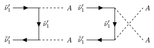
Figure 1: Annihilation channels for the dark matter particle $\tilde{\nu}^{\prime}_{1}$.

The particle $\tilde{\nu}^{\prime}_{1}$ is one of the twelve fermionic states which arise after ${\rm SU}(2)_{\ell}$ breaking and develop vector-like masses through the vacuum expectation values of $\hat{\Psi}_{1}$ and $\hat{\Psi}_{2}$. Due to the conservation of a remnant ${\rm U(1)}$ global symmetry Fornal et al. (2017) those fermions cannot decay exclusively to Standard Model particles. Therefore, the lightest of them remains stable and, if it is also electrically neutral, such as $\tilde{\nu}^{\prime}_{1}$, it becomes a good dark matter candidate. The Yukawa matrices can be chosen such that the non-dark matter fermions are heavy, whereas ${\tilde{\nu}^{\prime}_{1}}$ is light. As demonstrated in Fornal et al. (2017), the dark matter annihilation channel to lighter $CP$-odd scalars $A$ (see, Fig. 1),

$${\tilde{\nu}^{\prime}_{1}}\ {\bar{\tilde{\nu}}}^{\prime}_{1}\to A\ A\ ,$$ (27)

is sufficiently efficient to remove the symmetric component of dark matter. The remaining asymmetric component contributes to the observed dark matter relic abundance, as will be discussed in Section IV.

The breaking of the ${\rm SU}(4)$ symmetry also results in twelve fermionic states with vector-like masses, this time generated by the vacuum expectation value of $\hat{\Phi}$. Once again, because of the conservation of an accidental global ${\rm U}(1)$ symmetry Fornal et al. (2015), their decay channels cannot involve solely Standard Model particles in the final state. If the lightest of them is the electrically neutral $\tilde{u}^{\prime}_{1}$, it remains stable and becomes another viable component of dark matter. The annihilation channels leading to the correct relic abundance were discussed in Fornal et al. (2015), and in this case a successful asymmetric dark matter scenario can also be realized.

It is worth emphasizing that with two asymmetric dark matter candidates, their individual masses are not fixed by a single relic density requirement. Depending on the contribution of each of them to the relic abundance, one of them can have a mass smaller than the mass of the neutron, possibly introducing a connection to the dark matter models relevant for the neutron lifetime anomaly Fornal and Grinstein (2018).

IV Matter-antimatter asymmetry

The generation of a matter-antimatter imbalance in the model proceeds via two independent processes: leptogenesis and baryogenesis, both occurring in an asymmetric dark matter setting Nussinov (1985); Kaplan (1992); Hooper et al. (2005); Kaplan et al. (2009); Petraki and Volkas (2013); Zurek (2014). Leptogenesis, as demonstrated in Fornal et al. (2017), is realized through instantons during ${\rm SU}(2)_{\ell}$ breaking, whereas baryogenesis, as argued in Fornal et al. (2015), is achieved within the ${\rm SU}(4)$ sector through the effects of higher-dimensional operators. We discuss both mechanisms below.

The complete formula for the effective potential generated by $\hat{\Psi}_{1}$ and $\hat{\Psi}_{2}$ was derived in Fornal and Pierre (2022), where is was demonstrated that a first order phase transition from ${\rm SU}(2)_{\ell}$ breaking can occur. This scenario is realized in the model considered in this work, but happens at a higher symmetry breaking scale. Figure 2 shows a plot of the effective potential $V_{\rm eff}(\psi_{1},\psi_{2},T)$ produced using Mathematica Wolfram Research, Inc. , assuming the parameters $\lambda_{i}=0.001$, $v_{1}=v_{2}$, $v_{\Psi}=100\ \rm EeV$, $g_{\ell}=1$, at high temperature (red) and at low temperature (green). As the temperature drops, the potential develops new vacua with lower energy densities (see Fornal and Pierre (2022) for details), separated by a barrier from the high-temperature vacuum. This leads to a first order phase transition, which is precisely the out-of-equilibrium condition enabling leptogenesis to happen, and combines the framework of asymmetric dark matter with several other leptogenesis/baryogenesis mechanisms Dick et al. (2000); Murayama and Pierce (2002); Shu et al. (2007); Blennow et al. (2011).

There are four vacua of this type for the scalar potential $V_{\rm eff}(\psi_{1},\psi_{2})$, but since two of them are related through the gauge transformation $\Psi_{i}\to e^{i\theta}\Psi_{i}$, only two of the four vacua are physically distinct Ginzburg and Krawczyk (2005); Battye et al. (2011). We denote them by $\vec{\psi}_{\rm vac1}$ and $\vec{\psi}_{\rm vac2}$. The degeneracy between the energy densities of these vacua is broken by the $\mathcal{Z}_{2}$ symmetry breaking terms in the effective potential, primarily governed by the parameter $m_{12}^{2}$.

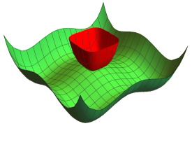
Figure 2: Effective potential of the model $V_{\rm eff}(\psi_{1},\psi_{2},T)$ at low temperature (green) and high temperature (red).

The first order phase transition corresponds to nucleation of bubbles with true vacuum inside. Outside the bubble the non-perturbative ${\rm SU}(2)_{\ell}$ instanton-induced processes described by Eq. (24) remain active. This, along with a sufficiently large amount of $CP$ violation (provided by the appropriate terms in the scalar potential for $\hat{\Psi}_{1}$ and $\hat{\Psi}_{2}$), leads to the generation of a lepton number excess. As the bubble expands, those regions get trapped inside the bubble, where lepton number violation no longer occurs, leading to the accumulation of lepton number in the Universe. Since the instantons also violate the global dark matter ${\rm U}(1)$ symmetry Fornal et al. (2017), this results in the generation of a dark matter asymmetry as well. This process is described by a set of twelve diffusion equations, which have the general form Joyce et al. (1996); Cohen et al. (1994)

$$\frac{\partial{\rho_{Ni}}}{\partial t}=D_{i}\nabla^{2}\rho_{Ni}-\sum_{j}\Gamma_{ij}\frac{\rho_{Nj}}{n_{j}}+\gamma_{i}\ .$$ (28)

In the expression above, $\rho_{Ni}$ is the particle number density, $D_{i}$ and $\Gamma_{ij}$ are the diffusion constant and rate, respectively, $n_{j}$ is the number of degrees of freedom, and $\gamma_{i}$ is the $i$-th $CP$-violating source given by Riotto (1996)

$$\gamma_{i}\approx\frac{\lambda_{7}\mu_{12}^{2}}{32\pi}\frac{\Gamma_{\psi_{i}}T_{*}}{m_{\psi_{i}}^{3}\!(T_{*})}\partial_{z}\psi_{i}\ ,$$ (29)

where $T_{*}$ is the bubble nucleation temperature, $\Gamma_{\psi_{i}}$ is the decay rate of $\psi_{i}$, the $z$-axis is in the direction perpendicular to the bubble wall, and $\mu_{12}^{2}={\rm Re}(m_{12}^{2})$. Solving the diffusion equations for our set of parameters reveals that the generated lepton asymmetry versus the dark matter asymmetry is

$$\frac{|\Delta L|}{|\Delta\tilde{\nu}^{\prime}_{1}|}=3\ ,$$ (30)

consistent with the existing result Fornal et al. (2017). The amount of lepton asymmetry produced in this process is subsequently altered by the electroweak sphalerons Harvey and Turner (1990), which partially convert it into a baryon asymmetry,

$$|\Delta B|=\frac{84}{79}|\Delta\tilde{\nu}^{\prime}_{1}|\ .$$ (31)

Assuming a bubble wall velocity equal to the speed of light, we find that for $v_{\Psi}=100\ {\rm EeV}$ and $\lambda_{i}\sim 10^{-4}$ the observed baryon-to-photon ratio Workman et al. (2022)

$$\eta\sim 6\times 10^{-10}$$ (32)

is generated provided that

$$|\lambda_{7}\mu_{12}^{2}|\,Y^{2}\sim 10^{-10}\ {\rm EeV^{2}}\ .$$ (33)

This condition can be satisfied by a wide range of parameter values, e.g., $\lambda_{7}\sim 10^{-6}$, $\mu_{12}^{2}\sim 10^{-2}\,{\rm EeV^{2}}$, and $Y\sim 10^{-1}$. The dark matter mass is then given by

$$m_{\tilde{\nu}^{\prime}_{1}}\approx\frac{\Omega_{\tilde{\nu}^{\prime}_{1}}}{\Omega_{B}}\frac{|\Delta B|}{|\Delta\tilde{\nu}^{\prime}_{1}|}\,m_{\rm proton}\ .$$ (34)

If the $\tilde{\nu}^{\prime}_{1}$ particle makes up all of the dark matter in the Universe, this condition implies $m_{\tilde{\nu}^{\prime}_{1}}\approx 5\ {\rm GeV}$. However, $\tilde{\nu}^{\prime}_{1}$ can be lighter if the dark matter in the Universe consists also of the $\tilde{u}^{\prime}_{1}$ particles.

Indeed, an analogous asymmetric dark matter mechanism can generate a contribution to the baryon and dark matter asymmetries in the $\rm SU(4)$ sector. As pointed out in Fornal et al. (2015), the following dimension-six operators,

$$\frac{c_{1}}{\Lambda^{2}}\epsilon_{abcd}\,\hat{u}^{a}_{R}\hat{u}^{b}_{R}\hat{d}^{c}_{R}\hat{d}^{d}_{R}\ ,\ \ \ \frac{c_{2}}{\Lambda^{2}}\epsilon_{abcd}\,(\hat{Q}^{a}_{L}\epsilon\,\hat{Q}^{b}_{L})(\hat{Q}^{c}_{L}\epsilon\,\hat{Q}^{d}_{L})\ ,\ \ \ \ \ \ \$$ (35)

violate baryon and dark matter number by one unit, and the initially produced asymmetries are related via $\Delta B_{i}=-\Delta\tilde{u}^{\prime}_{1}$. The baryon asymmetry is then depleted because of the effect of electroweak sphalerons to

$$|\Delta B|=\frac{28}{79}|\Delta\tilde{u}^{\prime}_{1}|\ .$$ (36)

The mass of the $\tilde{u}^{\prime}_{1}$ particle in such an asymmetric dark matter scenario is

$$m_{\tilde{u}^{\prime}_{1}}\approx\frac{\Omega_{\tilde{u}^{\prime}_{1}}}{\Omega_{B}}\frac{|\Delta B|}{|\Delta\tilde{u}^{\prime}_{1}|}\,m_{\rm proton}\ .$$ (37)

If all of the dark matter consists of the $\tilde{u}^{\prime}_{1}$ particles, then their mass is $m_{\tilde{u}^{\prime}_{1}}\approx 1.75\ {\rm GeV}$. However, similarly as before, this mass can be smaller if the $\tilde{\nu}^{\prime}_{1}$ particles also contribute.

With two dark matter candidates, the dark matter relic abundance is given by the sum of the two contributions

$$\Omega_{\rm DM}=\varepsilon\,\Omega_{\tilde{\nu}^{\prime}_{1}}+(1-\varepsilon)\,\Omega_{\tilde{u}^{\prime}_{1}}\ ,$$ (38)

where $\varepsilon$ can take any value between 0 and 1. Given the relations in Eqs. (34) and (37), one of the particles $\tilde{\nu}^{\prime}_{1}$ and $\tilde{u}^{\prime}_{1}$ can have a mass smaller than that of the neutron, introducing a possible connection to models proposed to explain the neutron lifetime puzzle Fornal and Grinstein (2018).

V Domain wall signatures

When the $\rm SU(2)_{\ell}$ symmetry is spontaneously broken, patches of the Universe undergo a first order phase transition to one of the vacua described earlier: $\vec{\psi}_{\rm vac1}$ or $\vec{\psi}_{\rm vac2}$. Since those two vacua correspond to disconnected manifolds, domain walls are create along their boundaries. The breaking of the $\mathcal{Z}_{2}$ symmetry between the vacua is essential, since without it domain walls would remain stable, leading to cosmological problems, as they would result in unacceptably large density fluctuations in the Universe Saikawa (2017).

In our model the $\mathcal{Z}_{2}$ symmetry is softly broken by the small $m_{12}^{2}$ term, so that the vacua $\vec{\psi}_{\rm vac1}$ and $\vec{\psi}_{\rm vac2}$ have slightly different energy densities. This introduces an instability of the created domain walls and leads to their annihilation, which in turn gives rise to a stochastic gravitational wave background. It is worth noting that for domain walls to actually form, the $\mathcal{Z}_{2}$ symmetry can only be softly broken, otherwise patches of the Universe would predominantly tunnel to the lower energy density state and no topological defects would arise.

V.1 Domain wall creation and annihilation

Choosing the $z$-axis to be perpendicular to the domain wall, the profile of the static configuration $\vec{\psi}_{dw}(z)$ is given by the solution of the equation

$$\frac{d^{2}\vec{\psi}_{dw}(z)}{dz^{2}}-\vec{\nabla}_{\!\psi}V_{\rm eff}\big{[}\vec{\psi}_{dw}(z)\big{]}=0\ ,$$ (39)

subject to the boundary conditions:

$$\vec{\psi}_{dw}(z=-\infty)=\vec{\psi}_{\rm vac1}\ ,\ \ \ \ \ \vec{\psi}_{dw}(z=\infty)=\vec{\psi}_{\rm vac2}\ .\ \ \ \ \ \ \$$ (40)

One of the domain wall parameters, which the resulting gravitational wave signal depends on, is the tension $\sigma$,

$$\sigma=\int_{-\infty}^{\infty}dz\,\rho_{dw}(z)\ ,$$ (41)

where $\rho_{dw}$ is the energy density of the domain wall,

$$\rho_{dw}(z)=\frac{1}{2}\bigg{(}\frac{d\vec{\psi}_{dw}(z)}{dz}\bigg{)}^{2}+V_{\rm eff}\big{[}\vec{\psi}_{dw}(z)\big{]}\ .$$ (42)

In our case the tension can be estimated as

$$\sigma\,\sim\,v_{\Psi}^{3}\ .$$ (43)

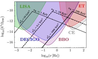
Figure 3: Gravitational wave signals from domain wall annihilation for several choices of parameters. The colored regions correspond to the reach of future gravitational wave experiments: LISA (green), Big Bang Observer (purple), DECIGO (blue), Einstein Telescope (red), and Cosmic Explorer (gray).

The second parameter governing the gravitational wave spectrum is the difference between the energy densities of the two vacua $\Delta\rho$ (also called the potential bias), which in our model can be approximated by

$$\Delta\rho\sim\mu_{12}^{2}v_{\Psi}^{2}\ .$$ (44)

If the potential bias in nonzero, the domain walls become unstable and annihilate when the volume pressure, $p_{V}\sim\Delta\rho$, exceeds the pressure due to tension, $p_{T}\sim{\sigma^{2}}/{M_{Pl}^{2}}$, where $M_{Pl}$ is the Planck mass. This implies the following condition on the parameters of our model,

$$\mu^{2}_{12}\gtrsim\frac{v_{\Psi}^{4}}{M_{Pl}^{2}}\ .$$ (45)

For example, if $v_{\Psi}\sim 100\ {\rm EeV}$ then for the domain walls to annihilate promptly one requires $\mu_{12}^{2}\gtrsim 1\ {\rm TeV^{2}}$, whereas for $v_{\Psi}\sim 1\ {\rm EeV}$ this bound is relaxed to $10^{-2}\ {\rm GeV^{2}}$. The additional constraint on $\mu_{12}^{2}$ assuring that domain wall annihilation happens before Big Bang nucleosynthesis (so that it does not alter the ratios of the produced elements) is much weaker.

V.2 Gravitational wave signal

The annihilation of domain walls gives rise to a stochastic gravitational wave background described by Kadota et al. (2015); Saikawa (2017),

$$h^{2}\Omega_{\rm DW}(\nu) \approx 7\times 10^{-21}\left(\frac{g_{*}}{100}\right)^{-\frac{1}{3}}\left(\frac{\sigma}{\rm EeV^{3}}\right)^{4}\left(\frac{\rm PeV^{4}}{\Delta\rho}\right)^{2}$$ (46)

$$\times \!\!\left[\left(\frac{\nu}{\nu_{d}}\right)^{3}\theta(\nu_{d}-\nu)+\left(\frac{\nu_{d}}{\nu}\right)\theta(\nu-\nu_{d})\right],\ \ \ \ \ \ \$$

where we adopted the values of the area parameter $\mathcal{A}=0.8$ and efficiency parameter $\tilde{\epsilon}_{\rm gw}=0.7$ Hiramatsu et al. (2014), $g_{*}$ is the number of degrees of freedom, $\theta(x)$ is the Heaviside step function, and $\nu_{d}$ is the peak frequency given by

$$\nu_{d}\approx(4.5\ {\rm Hz})\,\sqrt{\frac{\rm EeV^{3}}{\sigma}\frac{\Delta\rho}{\rm PeV^{4}}}\ .$$ (47)

As described by Eq. (46), the spectrum scales like $\sim\nu^{3}$ for frequencies below the peak frequency, and $\sim 1/\nu$ for higher frequencies. The constraints arising from the cosmic microwave background measurements impose the condition $h^{2}\Omega(\nu)<2.9\times 10^{-7}$ Clarke et al. (2020), which requires the parameters $v_{\Psi}$ and $\mu_{12}^{2}$ in our model to satisfy the relation

$$\frac{v_{\Psi}^{4}}{\mu^{2}_{12}}\lesssim(2.5\times 10^{9}\ \rm EeV)^{2}\ .$$ (48)

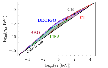
Figure 4: Parameter space regions where the gravitational wave signal from domain walls has a signal-to-noise ratio of at least five after one year of collecting data for various experiments. The black dots correspond to the three signatures shown in Fig. 3.

Figure 3 shows the expected gravitational wave signal from domain walls for several choices of model parameters, plotted over the sensitivity regions of future gravitational wave detectors: Laser Interferometer Space Antenna (LISA) Amaro-Seoane et al. (2017), Big Bang Observer (BBO) Crowder and Cornish (2005), DECIGO Kawamura et al. (2011), Einstein Telescope (ET) Punturo et al. (2010) and Cosmic Explorer (CE) Reitze et al. (2019). Figure 4 displays regions of parameter space for which the signal can be detected at those experiments – the upper bound on $\mu_{12}$ is detector-specific (the colors correspond to the selection made in Fig. 3), whereas the lower bound arises from the cosmic microwave background radiation constraint in Eq. (48).

VI Phase transition signatures

We consider now the possibility of having a first order phase transition associated with ${\rm SU}(4)$ breaking occurring at the PeV scale and producing a measurable gravitational wave signal. We first calculate the effective potential of the model. We then proceed to computing the parameters governing the dynamics of the bubble nucleation, and ultimately determine the shape of the possible gravitational wave signatures.

VI.1 Effective potential

Denoting the background field by $\phi$, the three contributions to the effective potential are: the tree-level term $V_{0}(\phi)$, the Coleman-Weinberg one-loop correction $V_{\rm CW}(\phi)$, and the finite temperature part $V_{T}(\phi,T)$, so that

$$V_{\rm eff}(\phi,T)=V_{0}(\phi)+V_{\rm CW}(\phi)+V_{T}(\phi,T)\ .$$ (49)

Substituting in Eq. (8) the value of $m_{\Phi}^{2}$ obtained from minimizing the potential, one obtains

$$V_{0}(\phi)=-\frac{1}{2}\lambda_{\Phi}v^{2}_{\Phi}\phi^{2}+\frac{1}{4}\lambda_{\Phi}\phi^{4}\ .$$ (50)

For the Coleman-Weinberg contribution, we use the cutoff regularization scheme and set the minimum of the zero temperature potential and the mass of $\phi$ to be equal to their tree-level values, which results in Anderson and Hall (1992)

$$V_{\rm CW}(\phi) = \sum_{i}\frac{n_{i}}{(8\pi)^{2}}\bigg{\{}m_{i}^{4}(\phi)\left[\log\left(\frac{m_{i}^{2}(\phi)}{m_{i}^{2}(v_{\Phi})}\right)-\frac{3}{2}\right]$$ (51)

$$+\ 2\,m_{i}^{2}(\phi)\,m_{i}^{2}(v_{\Phi})\bigg{\}}\ ,$$

where contributions from all particles charged under $\rm SU(4)$ are summed over, including $\chi$ (the Goldstone bosons), $n_{i}$ is the number of degrees of freedom, and $m_{i}$ are the background field-dependent masses (we substitute $m_{\chi}(v)\to m_{\Phi}(v)$ for the Goldstone bosons, where $\Phi$ is the radial mode). Those masses for the gauge bosons are

$$m_{G^{\prime}}(\phi) = \tfrac{1}{2}g_{4}\phi\ ,$$

$$m_{Z^{\prime}}(\phi) = \tfrac{1}{2}\sqrt{\tfrac{3}{2}g_{4}^{2}+g_{X}^{2}}\,\phi\ ,$$ (52)

and for the radial mode of the scalar $\hat{\Phi}$,

$$m_{\Phi}=\sqrt{2\lambda_{\Phi}}\,\phi\ .$$ (53)

The corresponding numbers of degrees of freedom are:$n_{G^{\prime}}=18$, $n_{Z^{\prime}}=3$, $n_{\Phi}=1$, and $n_{\chi}=7$.

Finally, the finite temperature part of the effective potential is given by Quiros (2007)

$$V_{T}(\phi,T) = \frac{T^{4}}{2\pi^{2}}\sum_{i}n_{i}\int_{0}^{\infty}dx\,x^{2}\log\left[1\mp e^{-\sqrt{x^{2}+\tfrac{m_{i}^{2}(\phi)}{T^{2}}}}\right]$$ (54)

$$+\,\frac{T}{12\pi}\sum_{k}n^{\prime}_{k}\left\{m_{k}^{3}(\phi)-\left[m_{k}^{2}(\phi)+\Pi_{k}(T)\right]^{3/2}\right\},$$

where the first line is generated by one-loop diagrams (the sum is over all particles), while the second line arises from the Daisy diagrams (the sum is over bosons only). The prime symbol indicates that only longitudinal degrees of freedom in the case of vector bosons are included (i.e., $n^{\prime}_{G^{\prime}}=6$, $n^{\prime}_{Z^{\prime}}=1$, $n^{\prime}_{\Phi}=1$, $n^{\prime}_{\chi}=7$), and $\Pi_{k}(T)$ are the thermal masses Comelli and Espinosa (1997), which in our model are calculated to be (for $\lambda_{\Phi}\ll 1$)

$$\Pi_{G^{\prime}}(T)=\Pi_{Z^{\prime}}(T)=\tfrac{8}{3}g_{4}^{2}\,T^{2}\ ,$$

$$\Pi_{\Phi}(T)=\Pi_{\chi}(T)=\tfrac{1}{16}\!\left(g_{X}^{2}+\tfrac{15}{2}g_{4}^{2}\right)T^{2}\ .$$ (55)

Figure 5 shows the resulting effective potential plotted adopting $v_{\Phi}=100\ \rm TeV$, the values of $g_{4}$ and $g_{X}$ at that scale (as discussed in Sec. II.3), and $\lambda_{\Phi}=0.004$. With decreasing temperature, a new true vacuum is formed with a lower energy density than the high temperature false vacuum. Since there is a potential barrier between the two minima, a first order phase transition becomes possible.

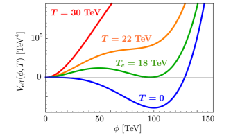
Figure 5: Effective potential of the $\rm SU(4)$ sector of the model, $V_{\rm eff}(\phi,T)$, assuming $v_{\Phi}=100\ \rm TeV$ and $\lambda_{\Phi}=0.004$, for several choices of temperature.

VI.2 Bubble nucleation

When the temperature drops below the so-called nucleation temperature $T_{*}$, this initiates the transition of various parts of the Universe from the false vacuum to the true one. Such first order phase transitions correspond to the nucleation of bubbles of true vacuum. The nucleation temperature can be determined from the condition that the bubble nucleation rate $\Gamma(T)$ becomes comparable to the Hubble expansion rate,

$$\Gamma(T_{*})\sim H(T_{*})^{4}\ .$$ (56)

The nucleation rate is given by Linde (1983)

$$\Gamma(T)\approx\left(\frac{S(T)}{2\pi T}\right)^{\frac{3}{2}}T^{4}e^{-{S(T)}/{T}}\ ,$$ (57)

in which $S(T)$ is the Euclidean action calculated as

$$S(T)=4\pi\int dr\,r^{2}\left[\frac{1}{2}\left(\frac{d\phi_{b}}{dr}\right)^{2}+V_{\rm eff}(\phi_{b},T)\right],\ \ \ \ \$$ (58)

where $\phi_{b}(r)$ is the bounce solution describing the profile of the expanding bubble, i.e., the solution to the equation

$$\frac{d^{2}\phi}{dr^{2}}+\frac{2}{r}\frac{d\phi}{dr}-\frac{d}{d\phi}V_{\rm eff}(\phi,T)=0\ ,$$ (59)

subject to the following boundary conditions:

$$\frac{d\phi}{dr}\bigg{|}_{r=0}=0\ ,\ \ \ \ \ \phi(\infty)=\phi_{\rm false}\ .$$ (60)

The nucleation temperature is calculated, using Eqs. (56) and (57), as the solution to the equation

$$\frac{S(T_{*})}{T_{*}}\approx 4\log\!\left[\frac{M_{Pl}}{T_{*}}\right]-2\log\left[\frac{4\pi^{3}g_{*}}{45}\!\left(\frac{2\pi\,T_{*}}{S(T_{*})}\right)^{\!\!\frac{3}{4}}\right].\ \ \ \ \ \$$ (61)

VI.3 Gravitational wave signal

During the nucleation and the violent expansion of bubbles of true vacuum, a stochastic gravitational wave background is generated via bubble wall collisions, sound shock waves in the primordial plasma, and magnetohydrodynamic turbulence. The shape of the spectrum is determined through simulations and depends only on four quantities: bubble wall velocity $v_{w}$ (assumed here to be equal to the speed of light; see Espinosa et al. (2010); Caprini et al. (2016) for more details), nucleation temperature $T_{*}$, strength of the phase transition $\alpha$, and duration of the phase transition $1/\tilde{\beta}$. Those parameters depend on the shape of the effective potential, which itself is specific to the particular particle physics model under investigation. This introduces a correspondence between the fundamental parameters of the Lagrangian and the resulting gravitational wave signal.

Upon determining the nucleation temperature $T_{*}$ by solving Eq. (61), the parameter $\alpha$ is calculated as

$$\alpha=\frac{\rho_{\rm vac}(T_{*})}{\rho_{\rm rad}(T_{*})}\ ,$$ (62)

i.e., as the ratio of the difference between the energy densities of the true and false vacua,

$$\rho_{\rm vac}(T) = V_{\rm eff}(\phi_{\rm false},T)-V_{\rm eff}(\phi_{\rm true},T)$$ (63)

$$- T\frac{\partial}{\partial T}{\Big{[}V_{\rm eff}(\phi_{\rm false},T)-V_{\rm eff}(\phi_{\rm true},T)\Big{]}},\ \ \ \ \ \$$

and the radiation energy density

$$\rho_{\rm rad}(T)=\frac{\pi^{2}}{30}g_{*}T^{4}\ .$$ (64)

The parameter $\tilde{\beta}$ is computed as

$$\tilde{\beta}=T_{*}\frac{d}{dT}\!\left[\frac{S(T)}{T}\right]\bigg{|}_{T=T_{*}}\ .$$ (65)

Based on numerical simulations, the contribution to the stochastic gravitational wave spectrum from sound waves is given by the empirical formula Hindmarsh et al. (2014); Caprini et al. (2016)

$$h^{2}\Omega_{\rm sound}(\nu)\, \approx \,\frac{1.9\times 10^{-5}}{\tilde{\beta}}\left(\frac{g_{*}}{100}\right)^{\!-\frac{1}{3}}\left(\frac{\alpha\,\kappa_{s}}{\alpha+1}\right)^{2}$$ (66)

$$\times \frac{(\nu/\nu_{s})^{3}}{\big{[}1+0.75\,(\nu/\nu_{s})^{2}\big{]}^{\frac{7}{2}}}\ \Upsilon\ ,$$

where the fraction of the latent heat transformed into the bulk motion of the plasma Espinosa et al. (2010) and the peak frequency are

$$\kappa_{s} = \frac{\alpha}{0.73+0.083\sqrt{\alpha}+\alpha}\ ,$$

$$\nu_{s} = (0.019\ {\rm Hz})\left(\frac{T_{*}}{100\ {\rm TeV}}\right)\left(\frac{g_{*}}{100}\right)^{\frac{1}{6}}\tilde{\beta}\ ,\ \ \ \ \ \ \$$ (67)

and the suppression factor is given by Ellis et al. (2020b); Guo et al. (2021)

$$\Upsilon=1-\frac{1}{\sqrt{1+\frac{8\pi^{1/3}}{\tilde{\beta}}\sqrt{\frac{\alpha+1}{3\alpha\kappa_{s}}}}}\ .\ \ \ \ \$$ (68)

The gravitational wave spectrum contribution from bubble wall collisions is estimated to be Kosowsky et al. (1992); Huber and Konstandin (2008); Caprini et al. (2016)

$$h^{2}\Omega_{\rm collision}(\nu)\, \approx \,\frac{4.9\times 10^{-6}}{\tilde{\beta}^{2}}\left(\frac{\alpha\,\kappa_{c}}{\alpha+1}\right)^{2}\left(\frac{g_{*}}{100}\right)^{\!-\frac{1}{3}}$$ (69)

$$\times \frac{(\nu/\nu_{c})^{2.8}}{1+2.8\,(\nu/\nu_{c})^{3.8}}\ ,$$

where the fraction of the latent heat deposited into the bubble front Kamionkowski et al. (1994) and the peak frequency are

$$\kappa_{c} = \frac{\frac{4}{27}\sqrt{\frac{3}{2}\alpha}+0.72\,\alpha}{1+0.72\,\alpha}\ ,$$

$$\nu_{c} = (0.0037\ {\rm Hz})\left(\frac{T_{*}}{100\ {\rm TeV}}\right)\left(\frac{g_{*}}{100}\right)^{\frac{1}{6}}\tilde{\beta}\ .\ \ \ \ \ \$$ (70)

Finally, magnetohydrodynamic turbulence adds the following contribution Caprini and Durrer (2006); Caprini et al. (2009),

$$h^{2}\Omega_{\rm turb}(\nu)\, \approx \,\frac{3.4\times 10^{-4}}{\tilde{\beta}}\left(\frac{\alpha\,\epsilon\,\kappa_{s}}{\alpha+1}\right)^{\frac{3}{2}}\left(\frac{g_{*}}{100}\right)^{-\frac{1}{3}}$$ (71)

$$\times \frac{({\nu}/{\nu_{t}})^{3}}{\big{(}1+{8\pi\,\nu}/{\nu_{*}}\big{)}\big{(}1+{\nu}/{\nu_{t}}\big{)}^{{11}/{3}}}\ ,$$

where the turbulence suppression parameter $\epsilon=0.05$ Caprini et al. (2016), the peak frequency is

$$\nu_{t} = (0.027\ {\rm Hz})\left(\frac{T_{*}}{100\ {\rm TeV}}\right)\left(\frac{g_{*}}{100}\right)^{\frac{1}{6}}{\tilde{\beta}}\ ,$$ (72)

and the parameter $\nu_{*}$ Caprini et al. (2016) is given by

$$\nu_{*}=(0.017\ {\rm Hz})\left(\frac{T_{*}}{100\ {\rm TeV}}\right)\left(\frac{g_{*}}{100}\right)^{\frac{1}{6}}\ .$$ (73)

The three contributions add up linearly, resulting in

$$h^{2}\Omega_{\rm PT}=h^{2}\Omega_{\rm sound}+h^{2}\Omega_{\rm collision}+h^{2}\Omega_{\rm turb}\ .\ \ \ \$$ (74)

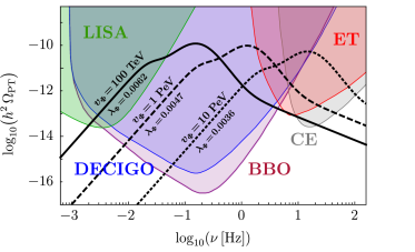
Figure 6: Gravitational wave signals from a first order phase transition for several choices of parameters. The colored regions correspond to the reach of future gravitational wave experiments, as in Fig. 3.

Lagrangian parameters				​Phase transition parameters​​
​​$v_{\Phi}\,[\rm TeV]$​​	$\lambda_{\Phi}$	$g_{4}$	$g_{X}$	$\alpha$	$\tilde{\beta}$	$T_{*}\,[\rm TeV]$
$100$	$0.0062$	$0.88$	$0.30$	9	220	$3.2$
$1000$	$0.0047$	$0.82$	$0.29$	30	260	$22$
$10000$	$0.0036$	$0.77$	$0.29$	43	350	$190$

Table 1: Phase transition and fundamental Lagrangian parameters for the three gravitational wave signatures presented in Fig. 6.

Figure 6 illustrates the gravitational wave signatures of the model arising from a first order phase transition in the early Universe for three different $\rm SU(4)$ symmetry breaking scales: $v_{\Phi}=100\ \rm TeV$ (solid line), $1\ \rm PeV$ (dashed line), and $10\ \rm PeV$ (dotted line), plotted for the quartic couplings $\lambda_{\Phi}$ which amplify the signal. In all of these cases the three contributions to the gravitational wave spectrum are visible: sound shock wave (main peak), bubble collision (to the left of the peak frequency), and magnetohydrodynamic turbulence (to the right of the peak). This is the result of the suppression factor $\Upsilon$ in Eq. (66), which reduces the contribution from sound waves roughly by a factor of 100 – without this suppression the gravitational wave signal would be dominated entirely by the sound wave component.

The translation between the fundamental Lagrangian parameters $(v_{\Phi},\lambda_{\Phi},g_{4},g_{Y})$ and the phase transition parameters $(T_{*},\alpha,\tilde{\beta})$ for each of the expected signals shown in Fig. 6 is provided in Table 1. The gauge couplings $g_{4}$ and $g_{Y}$ are fixed by the running of the Standard Model strong and electroweak couplings to have particular values at a given symmetry breaking scale, thus the only free fundamental parameters are $v_{\Phi}$ and $\lambda_{\Phi}$. The variation in the shape of the spectra shown in Fig. 6 arises precisely from the fact that the gauge couplings vary depending on the symmetry breaking scale – this affects the shape of the effective potential, thus different values of the quartic coupling $\lambda_{\Phi}$ are required to amplify the signal.

Phase transitions corresponding to a higher symmetry breaking scale are characterized by a larger nucleation temperature, which shifts the signal toward higher frequencies. A shift in the same direction occurs for transitions described by a larger parameter $\tilde{\beta}$. The height of the peak is determined by both the strength of the phase transition $\alpha$ and its duration $1/\tilde{\beta}$: the signal is stronger for larger values of $\alpha$ and for smaller values of $\tilde{\beta}$ (longer phase transitions).

In addition to the signals themselves, the sensitivities of the future gravitational wave experiments: LISA, DECIGO, Big Bang Observer, Einstein Telescope, and Cosmic Explorer, are also shown in Fig. 6. To investigate in more detail how this reach translates into probing the fundamental parameters in the Lagrangian, we scanned over $(v_{\Phi},\lambda_{\Phi})$ and determined the regions for which the above experiments will be sufficiently sensitive to detect the first order phase transition signals. The results of this scan are presented in Fig. 7.

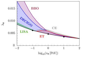
Figure 7: Parameter space regions where the gravitational wave signal from a first order phase transition has a signal-to-noise ratio of at least five after one year of collecting data for various experiments. The black dots correspond to the three signatures shown in Fig. 6.

VII Novel gravitational wave signature

An intriguing scenario arises when there is a large hierarchy between the $\rm SU(2)_{\ell}$ and $\rm SU(4)$ symmetry breaking scales. This offers the possibility of having the domain wall signal and the first order phase transition signal coexist, both being within the sensitivity region of upcoming gravitational wave experiments, and producing novel features to search for in the gravitational wave spectrum.

To realize this unique signature, we assume that the $\rm SU(2)_{\ell}$ symmetry is broken at the scale $v_{\Psi}\sim 100\ \rm EeV$, whereas the $\rm SU(4)$ is broken at $v_{\Phi}\sim 100\ \rm TeV$. The breaking of $\rm SU(2)_{\ell}$ at the high scale leads to the production of domain walls, which undergo annihilation (due to the small nonzero $\mu_{12}^{2}$ term) and produce a gravitational wave signal corresponding to the rightmost curve in Fig. 3. On the other hand, the $\rm SU(4)$ symmetry breaking at the lower scale results in a first order phase transition, which leads to a gravitational wave signal analogous to the leftmost curve in Fig. 6.

The two contributions combine to form a new double-bump gravitational wave signature shown in Fig. 8. The signal consists of a smooth peak arising from a first order phase transition, and a second sharp peak corresponding to domain wall annihilation. The slopes for the two peaks are different and are described by the frequency power law behavior in Eqs. (46), (66), (69), and (71), which can be used to differentiate between the two contributions.

Another promising property of the signal is that it can be searched for throughout a wide range of frequencies, making it relevant for a number of upcoming gravitational wave experiments: LISA, DECIGO, Big Bang Observer, Einstein Telescope, and Cosmic Explorer. Moreover, several parts of the spectrum can be probed by more than one experiment, which would foster collaboration between the different groups in case of a future discovery.

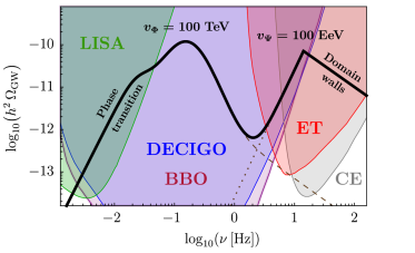
Figure 8: Novel gravitational wave signature of the model expected when a large hierarchy between symmetry breaking scales exists. The signal is searchable in future gravitational wave detectors: LISA, DECIGO, Big Bang Observer, Einstein Telescope, Cosmic Explorer.

VIII Summary and Outlook

Physics beyond the Standard Model is certainly necessary to explain several outstanding questions such as: What is dark matter? How did the matter-antimatter asymmetry originate? How do neutrino get their masses? In the time when conventional particle physics experiments, although working at the cutting edge of technological development and gathering extremely valuable data about the smallest and largest scales in the Universe, have not brought us answers to those questions, gravitational wave astronomy has provided us with a glimmer of hope to attack those problems from a new direction.

Processes taking place in the early Universe and triggered by new physics, such as first order phase transitions, domain wall annihilation, or the dynamics of cosmic strings, can produce a stochastic gravitational wave background detectable in current and future experiments, offering us precious insight into the particle physics at the highest energies. This makes analyzing models leading to such gravitational wave signals a worthwhile endeavor.

In this paper, we propose a particle physics framework which enables answering the aforementioned open questions and gives rise to a unique gravitational wave signature. The new model contains two dark matter candidates and allows to generate the matter-antimatter asymmetry of the Universe in an asymmetric dark matter setting through two distinct symmetry breaking events. Unlike in the case of typical asymmetric dark matter models, our scenario does not require the masses of the dark matter particles to be fixed at particular values. Depending on the individual contribution of each of them to the dark matter relic density, the mass of one of them can be below the mass of the neutron, opening up a possible connection to models explaining the neutron lifetime anomaly through a dark decay of the neutron Fornal and Grinstein (2018).

The new signature consists of two peaks: one arising from a first order phase transition triggered by $\rm SU(4)$ symmetry breaking at $\sim 100\ \rm TeV$, and the second one resulting from domain wall annihilation after $\rm SU(2)_{\ell}$ breaking at $\sim 100\ \rm EeV$. The signal spans a wide range of frequencies relevant for the upcoming gravitational wave experiments: LISA, DECIGO, Big Bang Observer, Einstein Telescope, and Cosmic Explorer. Since parts of the predicted signal lie in regions of overlapping sensitivities of various detectors, it also offers an opportunity of cross-checking the results, encouraging stronger collaboration within the gravitational wave physics community.

We note that several interesting variations of the proposed signature are possible. For example, the order of the two peaks may be reversed, which happens if the $\rm SU(2)_{\ell}$ is broken at $\sim 1\ \rm EeV$ while the $\rm SU(4)$ breaking occurs at $\sim 10\ \rm PeV$. Another intriguing scenario is when the peak frequencies of the two bumps coincide (when $\rm SU(2)_{\ell}$ is broken at $\sim 10\ \rm EeV$ and $\rm SU(4)$ is broken at $\sim 1\ \rm PeV$), leading to an unusual dependence on frequency in the signal peak region.

Finally, it would be interesting to investigate the possibility of an additional cosmic string contribution to the gravitational wave spectrum. Cosmic strings are typically produced when a $\rm U(1)$ gauge symmetry is spontaneously broken Kibble (1976), and the resulting gravitational wave signal depends on the scale at which this happens Vilenkin and Shellard (2000); Gouttenoire et al. (2020). However, it has recently been shown that cosmic strings can also be produced through the breaking of non-Abelian gauge symmetries. For example, if an $\rm SU(2)$ gauge group is broken by the vacuum expectation values of two triplet scalars (instead of the two doublets as in the model we considered), topologically stable strings can form Qaisar Shafi ; Hindmarsh et al. (2016). The interplay between the cosmic string contribution and other gravitational wave signatures will be the subject of an upcoming publication Bosch et al. .

A discovery of a stochastic gravitational wave background, such as the one discussed in this paper, would introduce a breakthrough in our understanding of the early Universe, shedding light on what happened just a small fraction of a second after the Big Bang.

Acknowledgments

This research was supported by the National Science Foundation under Grant No. PHY-2213144.

References

- Glashow (1961) S. L. Glashow, Partial Symmetries of Weak Interactions, Nucl. Phys. 22, 579–588 (1961).
- Higgs (1964) P. W. Higgs, Broken Symmetries and the Masses of Gauge Bosons, Phys. Rev. Lett. 13, 508–509 (1964).
- Englert and Brout (1964) F. Englert and R. Brout, Broken Symmetry and the Mass of Gauge Vector Mesons, Phys. Rev. Lett. 13, 321–323 (1964).
- Weinberg (1967) S. Weinberg, A Model of Leptons, Phys. Rev. Lett. 19, 1264–1266 (1967).
- Salam (1968) A. Salam, Weak and Electromagnetic Interactions, 8th Nobel Symposium Lerum, Sweden, May 19-25, 1968, Conf. Proc. C 680519, 367–377 (1968).
- Fritzsch et al. (1973) H. Fritzsch, M. Gell-Mann, and H. Leutwyler, Advantages of the Color Octet Gluon Picture, Phys. Lett. B 47, 365–368 (1973).
- Gross and Wilczek (1973) D. J. Gross and F. Wilczek, Ultraviolet Behavior of Nonabelian Gauge Theories, Phys. Rev. Lett. 30, 1343–1346 (1973).
- Politzer (1973) H. D. Politzer, Reliable Perturbative Results for Strong Interactions? Phys. Rev. Lett. 30, 1346–1349 (1973).
- Chatrchyan et al. (2012) S. Chatrchyan et al. (CMS), Observation of a New Boson at a Mass of 125 GeV with the CMS Experiment at the LHC, Phys. Lett. B 716, 30–61 (2012), arXiv:1207.7235 [hep-ex] .
- Aad et al. (2012) G. Aad et al. (ATLAS), Observation of a New Particle in the Search for the Standard Model Higgs Boson with the ATLAS Detector at the LHC, Phys. Lett. B 716, 1–29 (2012), arXiv:1207.7214 [hep-ex] .
- Rubin and Ford (1970) V. C. Rubin and Jr. Ford, W. K., Rotation of the Andromeda Nebula from a Spectroscopic Survey of Emission Regions, Astrophys. J. 159, 379 (1970).
- de Bernardis et al. (2000) P. de Bernardis et al. (Boomerang), A Flat Universe from High Resolution Maps of the Cosmic Microwave Background Radiation, Nature 404, 955–959 (2000), arXiv:astro-ph/0004404 .
- Gavazzi et al. (2007) R. Gavazzi, T. Treu, J. D. Rhodes, L. V. Koopmans, A. S. Bolton, S. Burles, R. Massey, and L. A. Moustakas, The Sloan Lens ACS Survey. 4. The Mass Density Profile of Early-Type Galaxies out to 100 Effective Radii, Astrophys. J. 667, 176–190 (2007), arXiv:astro-ph/0701589 .
- Feng (2010) J. L. Feng, Dark Matter Candidates from Particle Physics and Methods of Detection, Ann. Rev. Astron. Astrophys. 48, 495–545 (2010), arXiv:1003.0904 [astro-ph.CO] .
- Fornal et al. (2015) B. Fornal, A. Rajaraman, and T. M. P. Tait, Baryon Number as the Fourth Color, Phys. Rev. D 92, 055022 (2015), arXiv:1506.06131 [hep-ph] .
- Fornal et al. (2017) B. Fornal, Y. Shirman, T. M. P. Tait, and J. Rittenhouse West, Asymmetric Dark Matter and Baryogenesis from , Phys. Rev. D 96, 035001 (2017), arXiv:1703.00199 [hep-ph] .
- Nussinov (1985) S. Nussinov, Technocosmology? Could a Technibaryon Excess Provide a ?Natural? Missing Mass Candidate? Phys. Lett. B 165, 55–58 (1985).
- Kaplan (1992) D. B. Kaplan, A Single Explanation for Both the Baryon and Dark Matter Densities, Phys. Rev. Lett. 68, 741–743 (1992).
- Hooper et al. (2005) D. Hooper, J. March-Russell, and Stephen M. West, Asymmetric Sneutrino Dark Matter and the Puzzle, Phys. Lett. B 605, 228–236 (2005), arXiv:hep-ph/0410114 .
- Kaplan et al. (2009) D. E. Kaplan, M. A. Luty, and K. M. Zurek, Asymmetric Dark Matter, Phys. Rev. D 79, 115016 (2009), arXiv:0901.4117 [hep-ph] .
- Petraki and Volkas (2013) K. Petraki and R. R. Volkas, Review of Asymmetric Dark Matter, Int. J. Mod. Phys. A 28, 1330028 (2013), arXiv:1305.4939 [hep-ph] .
- Zurek (2014) K. M. Zurek, Asymmetric Dark Matter: Theories, Signatures, and Constraints, Phys. Rept. 537, 91–121 (2014), arXiv:1308.0338 [hep-ph] .
- Abbott et al. (2016) B. P. Abbott et al. (LIGO Scientific, Virgo), Observation of Gravitational Waves from a Binary Black Hole Merger, Phys. Rev. Lett. 116, 061102 (2016), arXiv:1602.03837 [gr-qc] .
- Amaro-Seoane et al. (2017) P. Amaro-Seoane et al. (LISA), Laser Interferometer Space Antenna, (2017), arXiv:1702.00786 [astro-ph.IM] .
- Crowder and Cornish (2005) J. Crowder and N. J. Cornish, Beyond LISA: Exploring Future Gravitational Wave Missions, Phys. Rev. D 72, 083005 (2005), arXiv:gr-qc/0506015 .
- Kawamura et al. (2011) S. Kawamura et al., The Japanese Space Gravitational Wave Antenna: DECIGO, Class. Quant. Grav. 28, 094011 (2011).
- Punturo et al. (2010) M. Punturo et al., The Einstein Telescope: A Third-Generation Gravitational Wave Observatory, Class. Quant. Grav. 27, 194002 (2010).
- Reitze et al. (2019) D. Reitze et al., Cosmic Explorer: The U.S. Contribution to Gravitational-Wave Astronomy beyond LIGO, Bull. Am. Astron. Soc. 51, 035 (2019), arXiv:1907.04833 [astro-ph.IM] .
- Kosowsky et al. (1992) A. Kosowsky, M. S. Turner, and R. Watkins, Gravitational Radiation from Colliding Vacuum Bubbles, Phys. Rev. D 45, 4514–4535 (1992).
- Turner (1997) M. S. Turner, Detectability of Inflation Produced Gravitational Waves, Phys. Rev. D 55, R435–R439 (1997), arXiv:astro-ph/9607066 .
- Hiramatsu et al. (2010) T. Hiramatsu, M. Kawasaki, and K. Saikawa, Gravitational Waves from Collapsing Domain Walls, JCAP 05, 032 (2010), arXiv:1002.1555 [astro-ph.CO] .
- Vachaspati and Vilenkin (1985) T. Vachaspati and A. Vilenkin, Gravitational Radiation from Cosmic Strings, Phys. Rev. D 31, 3052 (1985).
- Sakellariadou (1990) M. Sakellariadou, Gravitational Waves Emitted from Infinite Strings, Phys. Rev. D 42, 354–360 (1990), [Erratum: Phys. Rev. D 43, 4150 (1991)].
- Kibble (1976) T. W. B. Kibble, Topology of Cosmic Domains and Strings, J. Phys. A 9, 1387–1398 (1976).
- Eto et al. (2018a) M. Eto, M. Kurachi, and M. Nitta, Constraints on Two Higgs Doublet Models from Domain Walls, Phys. Lett. B 785, 447–453 (2018a), arXiv:1803.04662 [hep-ph] .
- Eto et al. (2018b) M. Eto, M. Kurachi, and M. Nitta, Non-Abelian Strings and Domain Walls in Two Higgs Doublet Models, JHEP 08, 195 (2018b), arXiv:1805.07015 [hep-ph] .
- Chen et al. (2020) N. Chen, T. Li, Z. Teng, and Y. Wu, Collapsing Domain Walls in the Two-Higgs-Doublet Model and Deep Insights from the EDM, JHEP 10, 081 (2020), arXiv:2006.06913 [hep-ph] .
- Battye et al. (2020) R. A. Battye, A. Pilaftsis, and D. G. Viatic, Domain Wall Constraints on Two-Higgs-Doublet Models with Symmetry, Phys. Rev. D 102, 123536 (2020), arXiv:2010.09840 [hep-ph] .
- Kadota et al. (2015) K. Kadota, M. Kawasaki, and K. Saikawa, Gravitational Waves from Domain Walls in the Next-to-Minimal Supersymmetric Standard Model, JCAP 10, 041 (2015), arXiv:1503.06998 [hep-ph] .
- Craig et al. (2021) N. Craig, I. Garcia Garcia, G. Koszegi, and A. McCune, P Not PQ, JHEP 09, 130 (2021), arXiv:2012.13416 [hep-ph] .
- Blasi et al. (2023) S. Blasi, A. Mariotti, A. Rase, A. Sevrin, and K. Turbang, Friction on ALP Domain Walls and Gravitational Waves, JCAP 04, 008 (2023), arXiv:2210.14246 [hep-ph] .
- Barman et al. (2022) B. Barman, D. Borah, A. Dasgupta, and A. Ghoshal, Probing High Scale Dirac Leptogenesis via Gravitational Waves from Domain Walls, Phys. Rev. D 106, 015007 (2022), arXiv:2205.03422 [hep-ph] .
- Borah and Dasgupta (2022) D. Borah and A. Dasgupta, Probing Left-Right Symmetry via Gravitational Waves from Domain Walls, Phys. Rev. D 106, 035016 (2022), arXiv:2205.12220 [hep-ph] .
- Borboruah and Yajnik (2022) Z. A. Borboruah and U. A. Yajnik, Left-Right Symmetry Breaking and Gravitational Waves : A Tale of Two Phase Transitions, (2022), arXiv:2212.05829 [astro-ph.CO] .
- Dunsky et al. (2021) D. I. Dunsky, A. Ghoshal, H. Murayama, Y. Sakakihara, and G. White, Gravitational Wave Gastronomy, (2021), arXiv:2111.08750 [hep-ph] .
- Moroi and Nakayama (2011) T. Moroi and K. Nakayama, Domain Walls and Gravitational Waves after Thermal Inflation, Phys. Lett. B 703, 160–166 (2011), arXiv:1105.6216 [hep-ph] .
- Saikawa (2017) K. Saikawa, A Review of Gravitational Waves from Cosmic Domain Walls, Universe 3, 40 (2017), arXiv:1703.02576 [hep-ph] .
- Grojean and Servant (2007) C. Grojean and G. Servant, Gravitational Waves from Phase Transitions at the Electroweak Scale and Beyond, Phys. Rev. D 75, 043507 (2007), arXiv:hep-ph/0607107 .
- Vaskonen (2017) V. Vaskonen, Electroweak Baryogenesis and Gravitational Waves from a Real Scalar Singlet, Phys. Rev. D 95, 123515 (2017), arXiv:1611.02073 [hep-ph] .
- Dorsch et al. (2017) G. C. Dorsch, S. J. Huber, T. Konstandin, and J. M. No, A Second Higgs Doublet in the Early Universe: Baryogenesis and Gravitational Waves, JCAP 05, 052 (2017), arXiv:1611.05874 [hep-ph] .
- Bernon et al. (2018) J. Bernon, L. Bian, and Y. Jiang, A New Insight into the Phase Transition in the Early Universe with Two Higgs Doublets, JHEP 05, 151 (2018), arXiv:1712.08430 [hep-ph] .
- Baldes and Servant (2018) I. Baldes and G. Servant, High Scale Electroweak Phase Transition: Baryogenesis and Symmetry Non-Restoration, JHEP 10, 053 (2018), arXiv:1807.08770 [hep-ph] .
- Chala et al. (2018) M. Chala, C. Krause, and G. Nardini, Signals of the Electroweak Phase Transition at Colliders and Gravitational Wave Observatories, JHEP 07, 062 (2018), arXiv:1802.02168 [hep-ph] .
- Alves et al. (2019) A. Alves, T. Ghosh, H.-K. Guo, K. Sinha, and D. Vagie, Collider and Gravitational Wave Complementarity in Exploring the Singlet Extension of the Standard Model, JHEP 04, 052 (2019), arXiv:1812.09333 [hep-ph] .
- Han et al. (2021) X.-F. Han, L. Wang, and Y. Zhang, Dark Matter, Electroweak Phase Transition, and Gravitational Waves in the Type II Two-Higgs-Doublet Model with a Singlet Scalar Field, Phys. Rev. D 103, 035012 (2021), arXiv:2010.03730 [hep-ph] .
- Benincasa et al. (2022) N. Benincasa, L. Delle Rose, K. Kannike, and L. Marzola, Multistep Phase Transitions and Gravitational Waves in the Inert Doublet Model, (2022), arXiv:2205.06669 [hep-ph] .
- Schwaller (2015) P. Schwaller, Gravitational Waves from a Dark Phase Transition, Phys. Rev. Lett. 115, 181101 (2015), arXiv:1504.07263 [hep-ph] .
- Breitbach et al. (2019) M. Breitbach, J. Kopp, E. Madge, T. Opferkuch, and P. Schwaller, Dark, Cold, and Noisy: Constraining Secluded Hidden Sectors with Gravitational Waves, JCAP 07, 007 (2019), arXiv:1811.11175 [hep-ph] .
- Croon et al. (2018) D. Croon, V. Sanz, and G. White, Model Discrimination in Gravitational Wave spectra from Dark Phase Transitions, JHEP 08, 203 (2018), arXiv:1806.02332 [hep-ph] .
- Hall et al. (2020) E. Hall, T. Konstandin, R. McGehee, H. Murayama, and G. Servant, Baryogenesis From a Dark First-Order Phase Transition, JHEP 04, 042 (2020), arXiv:1910.08068 [hep-ph] .
- Baldes (2017) I. Baldes, Gravitational Waves from the Asymmetric-Dark-Matter Generating Phase Transition, JCAP 05, 028 (2017), arXiv:1702.02117 [hep-ph] .
- Fornal and Pierre (2022) B. Fornal and E. Pierre, Asymmetric Dark Matter from Gravitational Waves, Phys. Rev. D 106, 115040 (2022), arXiv:2209.04788 [hep-ph] .
- Kierkla et al. (2023) M. Kierkla, A. Karam, and B. Swiezewska, Conformal Model for Gravitational Waves and Dark Matter: A Status Update, JHEP 03, 007 (2023), arXiv:2210.07075 [astro-ph.CO] .
- Dev et al. (2019) P. S. B. Dev, F. Ferrer, Y. Zhang, and Y. Zhang, Gravitational Waves from First-Order Phase Transition in a Simple Axion-Like Particle Model, JCAP 11, 006 (2019), arXiv:1905.00891 [hep-ph] .
- Von Harling et al. (2020) B. Von Harling, A. Pomarol, O. Pujolas, and F. Rompineve, Peccei-Quinn Phase Transition at LIGO, JHEP 04, 195 (2020), arXiv:1912.07587 [hep-ph] .
- Delle Rose et al. (2020) L. Delle Rose, G. Panico, M. Redi, and A. Tesi, Gravitational Waves from Supercool Axions, JHEP 04, 025 (2020), arXiv:1912.06139 [hep-ph] .
- Ferreira et al. (2022) R. Z. Ferreira, A. Notari, O. Pujolas, and F. Rompineve, High Quality QCD Axion at Gravitational Wave Observatories, Phys. Rev. Lett. 128, 141101 (2022), arXiv:2107.07542 [hep-ph] .
- Croon et al. (2019) D. Croon, T. E. Gonzalo, and G. White, Gravitational Waves from a Pati-Salam Phase Transition, JHEP 02, 083 (2019), arXiv:1812.02747 [hep-ph] .
- Huang et al. (2020) W.-C. Huang, F. Sannino, and Z.-W. Wang, Gravitational Waves from Pati-Salam Dynamics, Phys. Rev. D 102, 095025 (2020), arXiv:2004.02332 [hep-ph] .
- Okada et al. (2021) N. Okada, O. Seto, and H. Uchida, Gravitational Waves from Breaking of an Extra in Grand Unification, PTEP 2021, 033B01 (2021), arXiv:2006.01406 [hep-ph] .
- Ellis et al. (2020a) J. Ellis, M. Lewicki, and V. Vaskonen, Updated Predictions for Gravitational Waves Produced in a Strongly Supercooled Phase Transition, JCAP 11, 020 (2020a), arXiv:2007.15586 [astro-ph.CO] .
- Kawana (2022) K. Kawana, Cosmology of a Supercooled Universe, Phys. Rev. D 105, 103515 (2022), arXiv:2201.00560 [hep-ph] .
- Craig et al. (2020) N. Craig, N. Levi, A. Mariotti, and D. Redigolo, Ripples in Spacetime from Broken Supersymmetry, JHEP 21, 184 (2020), arXiv:2011.13949 [hep-ph] .
- Fornal et al. (2021) B. Fornal, B. Shams Es Haghi, J.-H. Yu, and Y. Zhao, Gravitational Waves from Mini-Split SUSY, Phys. Rev. D 104, 115005 (2021), arXiv:2104.00747 [hep-ph] .
- Brdar et al. (2019a) V. Brdar, L. Graf, A. J. Helmboldt, and X.-J. Xu, Gravitational Waves as a Probe of Left-Right Symmetry Breaking, JCAP 12, 027 (2019a), arXiv:1909.02018 [hep-ph] .
- Graf et al. (2022) L. Graf, S. Jana, A. Kaladharan, and S. Saad, Gravitational Wave Imprints of Left-Right Symmetric Model with Minimal Higgs Sector, JCAP 05, 003 (2022), arXiv:2112.12041 [hep-ph] .
- Brdar et al. (2019b) V. Brdar, A. J. Helmboldt, and J. Kubo, Gravitational Waves from First-Order Phase Transitions: LIGO as a Window to Unexplored Seesaw Scales, JCAP 02, 021 (2019b), arXiv:1810.12306 [hep-ph] .
- Okada and Seto (2018) N. Okada and O. Seto, Probing the Seesaw Scale with Gravitational Waves, Phys. Rev. D 98, 063532 (2018), arXiv:1807.00336 [hep-ph] .
- Di Bari et al. (2021) P. Di Bari, D. Marfatia, and Y.-L. Zhou, Gravitational Waves from First-Order Phase Transitions in Majoron Models of Neutrino Mass, JHEP 10, 193 (2021), arXiv:2106.00025 [hep-ph] .
- Zhou et al. (2022) R. Zhou, L. Bian, and Y. Du, Electroweak Phase Transition and Gravitational Waves in the Type-II Seesaw Model, JHEP 08, 205 (2022), arXiv:2203.01561 [hep-ph] .
- Hasegawa et al. (2019) T. Hasegawa, N. Okada, and O. Seto, Gravitational Waves from the Minimal Gauged Model, Phys. Rev. D 99, 095039 (2019), arXiv:1904.03020 [hep-ph] .
- Fornal and Shams Es Haghi (2020) B. Fornal and B. Shams Es Haghi, Baryon and Lepton Number Violation from Gravitational Waves, Phys. Rev. D 102, 115037 (2020), arXiv:2008.05111 [hep-ph] .
- Greljo et al. (2020) A. Greljo, T. Opferkuch, and B. A. Stefanek, Gravitational Imprints of Flavor Hierarchies, Phys. Rev. Lett. 124, 171802 (2020), arXiv:1910.02014 [hep-ph] .
- Fornal (2021) B. Fornal, Gravitational Wave Signatures of Lepton Universality Violation, Phys. Rev. D 103, 015018 (2021), arXiv:2006.08802 [hep-ph] .
- Dasgupta et al. (2022) A. Dasgupta, P. S. B. Dev, A. Ghoshal, and A. Mazumdar, Gravitational Wave Pathway to Testable Leptogenesis, Phys. Rev. D 106, 075027 (2022), arXiv:2206.07032 [hep-ph] .
- Badger et al. (2023) C. Badger, B. Fornal, K. Martinovic, A. Romero, K. Turbang, H. Guo, A. Mariotti, M. Sakellariadou, A. Sevrin, F.-W. Yang, and Y. Zhao, Probing Early Universe Supercooled Phase Transitions with Gravitational Wave Data, Phys. Rev. D 107, 023511 (2023), arXiv:2209.14707 [hep-ph] .
- Caldwell et al. (2022) R. Caldwell et al., Detection of Early-Universe Gravitational-Wave Signatures and Fundamental Physics, Gen. Rel. Grav. 54, 156 (2022), arXiv:2203.07972 [gr-qc] .
- Fornal and Grinstein (2018) B. Fornal and Be. Grinstein, Dark Matter Interpretation of the Neutron Decay Anomaly, Phys. Rev. Lett. 120, 191801 (2018), [Erratum: Phys.Rev.Lett. 124, 219901 (2020)], arXiv:1801.01124 [hep-ph] .
- (89) Wolfram Research, Inc., Wolfram Programming Lab, Version 13.2, Champaign, IL, 2023 .
- Dick et al. (2000) K. Dick, M. Lindner, M. Ratz, and D. Wright, Leptogenesis with Dirac Neutrinos, Phys. Rev. Lett. 84, 4039–4042 (2000), arXiv:hep-ph/9907562 .
- Murayama and Pierce (2002) H. Murayama and A. Pierce, Realistic Dirac Leptogenesis, Phys. Rev. Lett. 89, 271601 (2002), arXiv:hep-ph/0206177 .
- Shu et al. (2007) J. Shu, T. M. P. Tait, and C. E. M. Wagner, Baryogenesis from an Earlier Phase Transition, Phys. Rev. D 75, 063510 (2007), arXiv:hep-ph/0610375 .
- Blennow et al. (2011) M. Blennow, B. Dasgupta, E. Fernandez-Martinez, and N. Rius, Aidnogenesis via Leptogenesis and Dark Sphalerons, JHEP 03, 014 (2011), arXiv:1009.3159 [hep-ph] .
- Ginzburg and Krawczyk (2005) I. F. Ginzburg and M. Krawczyk, Symmetries of Two Higgs Doublet Model and CP Violation, Phys. Rev. D 72, 115013 (2005), arXiv:hep-ph/0408011 .
- Battye et al. (2011) R. A. Battye, G. D. Brawn, and A. Pilaftsis, Vacuum Topology of the Two Higgs Doublet Model, JHEP 08, 020 (2011), arXiv:1106.3482 [hep-ph] .
- Joyce et al. (1996) M. Joyce, T. Prokopec, and N. Turok, Nonlocal Electroweak Baryogenesis. Part 1: Thin Wall Regime, Phys. Rev. D 53, 2930–2957 (1996), arXiv:hep-ph/9410281 .
- Cohen et al. (1994) A. G. Cohen, D. B. Kaplan, and A. E. Nelson, Diffusion Enhances Spontaneous Electroweak Baryogenesis, Phys. Lett. B 336, 41–47 (1994), arXiv:hep-ph/9406345 .
- Riotto (1996) A. Riotto, Towards a Nonequilibrium Quantum Field Theory Approach to Electroweak Baryogenesis, Phys. Rev. D 53, 5834–5841 (1996), arXiv:hep-ph/9510271 .
- Harvey and Turner (1990) J. A. Harvey and M. S. Turner, Cosmological Baryon and Lepton Number in the Presence of Electroweak Fermion Number Violation, Phys. Rev. D 42, 3344–3349 (1990).
- Workman et al. (2022) R. L. Workman et al. (Particle Data Group), Review of Particle Physics, PTEP 2022, 083C01 (2022).
- Hiramatsu et al. (2014) T. Hiramatsu, M. Kawasaki, and K. Saikawa, On the Estimation of Gravitational Wave Spectrum from Cosmic Domain Walls, JCAP 02, 031 (2014), arXiv:1309.5001 [astro-ph.CO] .
- Clarke et al. (2020) T. J. Clarke, E. J. Copeland, and A. Moss, Constraints on Primordial Gravitational Waves from the Cosmic Microwave Background, JCAP 10, 002 (2020), arXiv:2004.11396 [astro-ph.CO] .
- Anderson and Hall (1992) G. W. Anderson and L. J. Hall, The Electroweak Phase Transition and Baryogenesis, Phys. Rev. D 45, 2685–2698 (1992).
- Quiros (2007) M. Quiros, Field Theory at Finite Temperature and Phase Transitions, Acta Phys. Polon. B 38, 3661–3703 (2007).
- Comelli and Espinosa (1997) D. Comelli and J. R. Espinosa, Bosonic Thermal Masses in Supersymmetry, Phys. Rev. D 55, 6253–6263 (1997), arXiv:hep-ph/9606438 .
- Linde (1983) A. D. Linde, Decay of the False Vacuum at Finite Temperature, Nuclear Physics B 216, 421 – 445 (1983).
- Espinosa et al. (2010) J. R. Espinosa, T. Konstandin, J. M. No, and G. Servant, Energy Budget of Cosmological First-Order Phase Transitions, JCAP 06, 028 (2010), arXiv:1004.4187 [hep-ph] .
- Caprini et al. (2016) C. Caprini et al., Science with the Space-Based Interferometer eLISA. II: Gravitational Waves from Cosmological Phase Transitions, JCAP 04, 001 (2016), arXiv:1512.06239 [astro-ph.CO] .
- Hindmarsh et al. (2014) M. Hindmarsh, S. J. Huber, K. Rummukainen, and D. J. Weir, Gravitational Waves from the Sound of a First Order Phase Transition, Phys. Rev. Lett. 112, 041301 (2014), arXiv:1304.2433 [hep-ph] .
- Ellis et al. (2020b) J. Ellis, M. Lewicki, and J. M. No, Gravitational Waves from First-Order Cosmological Phase Transitions: Lifetime of the Sound Wave Source, JCAP 07, 050 (2020b), arXiv:2003.07360 [hep-ph] .
- Guo et al. (2021) H.-K. Guo, K. Sinha, D. Vagie, and G. White, Phase Transitions in an Expanding Universe: Stochastic Gravitational Waves in Standard and Non-Standard Histories, JCAP 01, 001 (2021), arXiv:2007.08537 [hep-ph] .
- Huber and Konstandin (2008) S. J. Huber and T. Konstandin, Gravitational Wave Production by Collisions: More Bubbles, JCAP 09, 022 (2008), arXiv:0806.1828 [hep-ph] .
- Kamionkowski et al. (1994) M. Kamionkowski, A. Kosowsky, and M. S. Turner, Gravitational Radiation from First Order Phase Transitions, Phys. Rev. D 49, 2837–2851 (1994), arXiv:astro-ph/9310044 .
- Caprini and Durrer (2006) C. Caprini and R. Durrer, Gravitational Waves from Stochastic Relativistic Sources: Primordial Turbulence and Magnetic Fields, Phys. Rev. D 74, 063521 (2006), arXiv:astro-ph/0603476 .
- Caprini et al. (2009) C. Caprini, R. Durrer, and G. Servant, The Stochastic Gravitational Wave Background from Turbulence and Magnetic Fields Generated by a First-Order Phase Transition, JCAP 12, 024 (2009), arXiv:0909.0622 [astro-ph.CO] .
- Vilenkin and Shellard (2000) A. Vilenkin and E. P. S. Shellard, Cosmic Strings and Other Topological Defects, Cambridge University Press (2000).
- Gouttenoire et al. (2020) Y. Gouttenoire, G. Servant, and P. Simakachorn, Beyond the Standard Models with Cosmic Strings, JCAP 07, 032 (2020), arXiv:1912.02569 [hep-ph] .
- (118) Qaisar Shafi, Private communication .
- Hindmarsh et al. (2016) M. Hindmarsh, K. Rummukainen, and D. J. Weir, New Solutions for Non-Abelian Cosmic Strings, Phys. Rev. Lett. 117, 251601 (2016), arXiv:1607.00764 [hep-th] .
- (120) J. Bosch, Z. Delgado, B. Fornal, and A. Leon, Manuscript in preparation .