Guo et al.

Markov $\alpha$-Potential Games: Equilibrium Approximation and Regret Analysis

Markov $\alpha$-Potential Games: Equilibrium Approximation and Regret Analysis

Xin Guo,^a Xinyu Li,^a,* Chinmay Maheshwari,^b,* Shankar Sastry,^b Manxi Wu^c

${}^{\text{a}}$IEOR, UC Berkeley, CA, ${}^{\text{b}}$EECS, UC Berkeley, CA, ${}^{\text{c}}$ORIE, Cornell University, NY

^∗Corresponding author

Contact: xinguo@berkeley.edu, xinyu_li@berkeley.edu, chinmay_maheshwari@berkeley.edu, shankar_sastry@berkeley.edu, manxiwu@cornell.edu

This paper proposes a new notion of Markov $\alpha$-potential games to study Markov games. Two important classes of practically significant Markov games, Markov congestion games and the perturbed Markov team games, are analyzed in this framework of Markov $\alpha$-potential games, with explicit characterization of the upper bound for $\alpha$ and its relation to game parameters. Moreover, any maximizer of the $\alpha$-potential function is shown to be an $\alpha$-stationary Nash equilibrium of the game. Furthermore, two algorithms for the Nash regret analysis, namely the projected gradient-ascent algorithm and the sequential maximum improvement algorithm, are presented and corroborated by numerical experiments.

91A15, 91A25, 91A50, 91A06

Game Theory

Markov $\alpha$-potential games; Markov potential games; Multi-agent reinforcement learning; Nash-regret; Markov congestion games; Perturbed Markov team games; Projected gradient-ascent algorithm; Sequential maximum improvement.

1 Introduction

Markov potential games (MPG) are a class of Markov games, first proposed by Macua et al. [17] and further generalized by Leonardos et al. [15], as a framework to study multi-agent interactions in Markov games. In MPGs, the change in the utility function of any player who unilaterally deviates from her policy can be evaluated by the change in the value of a potential function. There is a rich literature studying various learning algorithms and their convergence properties for MPGs (Maheshwari et al. [18], Zhang et al. [31], Song et al. [26], Mao et al. [19], Ding et al. [11], Fox et al. [12], Zhang et al. [30], Marden [20], Macua et al. [17], Narasimha et al. [22]). However, the issues of verifying a Markov game being an MPG and the construction of its potential function remain largely unsolved, except for very few cases with restrictive assumptions, for example, when the state transition matrix is independent of players’ actions or when all players have identical payoff functions (Narasimha et al. [22], Leonardos et al. [15]). As a result, applications of the MPG framework to multi-agent interaction in practical settings remain limited.

Markov $\alpha$-potential games.

In this paper, we propose a new notion of Markov $\alpha$-potential game to study multi-agent games in dynamic settings. Markov $\alpha$-potential game is a generalization of MPG in the sense that any MPG is a Markov $\alpha$-potential game with $\alpha=0$.

We identify and analyze two classes of practically significant games as Markov $\alpha$-potential games. The first is the Markov congestion game (MCG), an extension of the well-known static congestion games proposed in Rosenthal [24] to the dynamic setting. MCGs can be used to model multi-agent systems such as dynamic routing in traffic, communication networks, and robotic interactions. The second is the perturbed Markov team game (PMTG), which generalizes the extensively studied Markov team game (Baudin and Laraki [6], Arslan and Yüksel [3], Sayin and Unlu [25], Wang and Sandholm [28], Panait and Luke [23], Yongacoglu et al. [29]) to accommodate the deviation of utility for any individual player from the team objective. For both classes of games, we explicitly characterize the upper bound of $\alpha$ (Propositions 3.1 and 3.2) and analyze its relation with respect to the game parameters. For MCGs, for instance, the upper bound of $\alpha$ is shown to scale inversely with the number of players (Proposition 3.1); for PMTGs, the upper bound of $\alpha$ decreases in the magnitude of payoff perturbation (Proposition 3.2).

Moreover, we construct a semi-infinite linear program to find an upper bound of $\alpha$ for any given Markov game. As a by-product, this program may be used to verify if a Markov game is a MPG. In addition, we show that any maximizer of the $\alpha$-potential function is an $\alpha$-stationary Nash equilibrium of the Markov $\alpha$-potential game (Proposition 3.3).

Furthermore, we propose two algorithms to approximate stationary Nash equilibrium in Markov $\alpha$-potential games. The first algorithm, Algorithm 1, is a projected gradient-ascent algorithm, which has been previously studied in the context of MPG (Ding et al. [11] ). The second algorithm, Algorithm 2, is new and called the sequential maximum improvement algorithm. For both algorithms, we derive their respective Nash-regret and its dependence on $\alpha$ (Theorem 4.1 and Theorem 4.2). For Algorithm 1, our analysis is built on the Nash-regret analysis of the projected gradient-ascent algorithm presented in Ding et al. [11] for MPGs, with additional analysis for the optimal step size to account for $\alpha$. For Algorithm 2, a crucial technical step in our analysis is to study the path length of policy updates, which is bounded in terms of the change of $\alpha$-potential function. The Nash-regret analysis of Algorithm 1 and Algorithm 2 applies to MPGs by setting $\alpha=0$. These regret-bound analyses highlight the flexibility of the Markov $\alpha$-potential game framework for studying general Markov games (Remarks 3.1 and 4.4). These results are corroborated with numerical studies.

Related works.

The generalization of Markov potential games to Markov $\alpha$-potential games is analogous to the extension of potential games to near-potential games (Candogan et al. [9, 7]) for static games. However, the extension in the dynamic setting poses several challenges. First, the expected utility function of any player in a static game is linear in the player’s mixed strategy, whereas in Markov games, players’ value functions may be nonlinear with respect to their policies due to the state transitions. As a result, the construction of the nearest potential function of a static game can be computed by a finite linear program, while the computation of $\alpha$ and the $\alpha$-potential function requires solving a semi-infinite linear program. Secondly, the convergence analysis of learning algorithms in Markov games requires different techniques compared to that in static games because of the Markov state transition and the non-myopic nature of players. Finally, the analysis of learning dynamics in static near-potential games primarily focuses on the asymptotic convergence guarantees, whereas in Markov games, the regret analysis captures the non-asymptotic convergence rate (Candogan et al. [9], Aydın et al. [4], Aydın and Eksin [5], Anagnostides et al. [2]).

Meanwhile, MCGs, the particular class of games studied in our work are closely related to the Markov state-wise potential games (Marden [20], Narasimha et al. [22]), where each state corresponds to a static potential game, and the state transition is Markovian. However, the analysis in (Marden [20], Narasimha et al. [22]) cannot be directly applied to the study of MCGs. In Marden [20], the players are assumed to be myopic and only maximize their one-stage payoff, whereas players in MCG model considered in this paper are long-run utility maximizers. Narasimha et al. [22] proposed several conditions for a Markov state-wise potential game to be an MPG, but these conditions are restrictive and require independence of the state transition matrix from either the current action profile or the state realization, as well as the separability of players’ utilities in state and action. In contrast, our analysis of MCGs imposes no such restrictions on either the state transition or the utility structure. Additionally, a recent work by Cui et al. [10] introduces an approximation algorithm for MCGs and investigates the Nash-regret. However, their approach specifically considers Markov games with a finite time horizon and independent state transitions. This is fundamentally different from the infinite time horizon games examined here, where no assumptions are made regarding the structure of state evolution. Furthermore, the results in Cui et al. [10] are tailored exclusively for congestion games, whereas our work focuses on a broader framework of Markov $\alpha$-potential games.

2 Setup

Consider a Markov game $\mathcal{G}=\langle I,S,(A_{i})_{i\in I},(u_{i})_{i\in I},P,\delta\rangle$, where $I$ is a finite set of players $i$; $S$ is a finite set of states $s$; $A_{i}$ is a finite set of actions with action $a_{i}$ for each player $i\in I$; $a=(a_{i})_{i\in I}\in A=\times_{i\in I}A_{i}$ is the action profile of all players; $u_{i}:S\times A\to\mathbb{R}$ such that $u_{i}(s,a)$ is the one-stage payoff for player $i$ with state $s\in S$ and action profile $a\in A$; $P=(P(s^{\prime}|s,a))_{s,s^{\prime}\in S,a\in A}$ is the probability transition matrix, where $P(s^{\prime}|s,a)$ is the one-step probability that the state changes from $s$ to $s^{\prime}$ with action profile $a$; and $\delta\in(0,1)$ is the discount factor. Let $\Delta(A_{i})$ represent the probability simplex over the action set $A_{i}.$ We consider a stationary Markov policy $\pi_{i}=(\pi_{i}(s,a_{i}))_{s\in S,a_{i}\in A_{i}}\in\Pi_{i}:=\Delta(A_{i})^{|S|}$, where $\pi_{i}(s,a_{i})$ is the probability that player $i$ chooses an action $a_{i}$ given state $s$; denote $\pi_{i}(s)=(\pi_{i}(s,a_{i}))_{a_{i}\in A_{i}}$ for each $i\in I$ and each $s\in S$; denote the joint policy profile as $\pi=(\pi_{i})_{i\in I}\in\Pi:=\times_{i\in I}\Pi_{i}$, and the joint policy of all players except player $i$ as $\pi_{-i}=(\pi_{j})_{j\in I\setminus\{i\}}\in\Pi_{-i}:=\times_{j\in I\setminus\{i\}}\Pi_{j}$. Additionally, denote the class of measurable functions on $S\times\Pi$ as $\mathcal{F}=\{f:S\times\Pi\rightarrow\mathbb{R}\}$; denote $\bar{A}=\max_{i\in I}|A_{i}|$ and $C=\max_{i\in I,s\in S,a\in A}u_{i}(s,a)$. The game proceeds in discrete time steps indexed by $k=\{0,1,2,...\}$. Given a stationary policy profile $\pi$ and an initial state distribution $\mu\in\Delta(S)$, where $\Delta(S)$ represents the probability simplex over state space $S$, the initial state $s^{0}$ at $k=0$ is sampled from $\mu$. At every step $k$, given the state $s^{k}$, each player $i$’s action $a^{k}_{i}\in A_{i}$ is realized from the policy $\pi_{i}(s^{k})$, and the realized action profile is $a^{k}=(a^{k}_{i})_{i\in I}$. The expected total discounted payoff for each player $i\in I$ is given by $V_{i}(\mu,\pi)=\mathbb{E}_{\mu,\pi}\left[\sum_{k=0}^{\infty}\delta^{k}u_{i}(s^{k},a^{k})\right]$ where $s^{0}\sim\mu$, $a^{k}\sim\pi(s^{k})$, and $s^{k}\sim P(\cdot|s^{k-1},a^{k-1})$. For the rest of the article, with a slight abuse of notation, $V_{i}(s,\pi)$ is used to denote the expected total payoff for player $i$ when the initial state is a fixed state $s\in S$, and $P^{\pi}(\cdot|\cdot)$ denotes the transition probability given the policy $\pi$, i.e., $P^{(\pi_{i},\pi_{-i})}(s^{\prime}|s)=\sum_{a_{-i}\in A_{-i}}\sum_{a_{i}\in A_{i}}\pi_{-i}(s,a_{-i})\pi_{i}(s,a_{i})P(s^{\prime}|s,a)$. The discounted state visitation distribution, for every $s\in S$, is defined as $d_{\mu}^{\pi}(s)=(1-\delta)\sum_{k=0}^{\infty}\delta^{k}P(s^{k}=s|s^{0}\sim\mu)$. Let $\kappa_{\mu}$ denote the maximum distribution mismatch of $\pi$ relative to $\mu$, and let $\tilde{\kappa}_{\mu}$ denote the minimax value of the distribution mismatch of $\pi$ relative to $\mu$. That is,

$$\kappa_{\mu}:=\sup_{\pi\in\Pi}\left\|d_{\mu}^{\pi}/\mu\right\|_{\infty},\quad\tilde{\kappa}_{\mu}:=\inf_{\nu\in\Delta(\mathcal{S})}\sup_{\pi\in\Pi}\|d_{\mu}^{\pi}/\nu\|_{\infty},$$ (1)

where the division $d_{\mu}^{\pi}/\nu$ is evaluated in a component-wise manner.

3 Markov $\alpha$-potential games

This section introduces the notion of Markov $\alpha$-potential games, and presents the properties of stationary Nash equilibrium in this game framework. To begin with, recall the definition of Markov potential games proposed by Leonardos et al. [15].

Definition 3.1 (Markov potential games (Leonardos et al. [15]))

A Markov game $\mathcal{G}$ is a Markov potential game if there exists a potential function $\Phi\in\mathcal{F}$ such that for any $i\in I$, $s\in S$, $\pi_{i},\pi_{i}^{\prime}\in\Pi_{i}$, and $\pi_{-i}\in\Pi_{-i}$,

$$\Phi(s,\pi_{i}^{\prime},\pi_{-i})-\Phi(s,\pi_{i},\pi_{-i})=V_{i}(s,\pi_{i}^{\prime},\pi_{-i})-V_{i}(s,\pi_{i},\pi_{-i}).$$ (2)

That is, a game is an MPG if there exists a potential function such that when a player unilaterally deviates from her policy, the change of the potential function is equal to the change of her expected payoff. As pointed out earlier, a key shortcoming of the MPG framework is the difficulty (Narasimha et al. [22]) to check the existence or to compute $\Phi$, thus limiting the scope of its real-world applications.

Instead, we propose to relax the equality in (2) to allow the difference between the change of any player’s payoff from unilateral deviation and the change of the potential function to be bounded by some $\alpha\geq 0$, under the notion of Markov $\alpha$-potential games. More precisely,

Definition 3.2 (Markov $\alpha$-potential game)

A Markov game $\mathcal{G}$ is a Markov $\alpha$-potential game for some $\alpha\geq 0$ such that

$$\alpha:=\inf_{\Psi\in\mathcal{F}}\sup_{s\in S,i\in I,\pi_{i},\pi^{\prime}_{i}\in\Pi_{i},\pi_{-i}\in\Pi_{-i}}\left|\Psi\left(s,\pi_{i}^{\prime},\pi_{-i}\right)-\Psi\left(s,\pi_{i},\pi_{-i}\right)-\left(V_{i}\left(s,\pi_{i}^{\prime},\pi_{-i}\right)-V_{i}\left(s,\pi_{i},\pi_{-i}\right)\right)\right|.$$ (3)

We call $\Phi\in\mathcal{F}$ as an $\alpha$-potential function if

$$\alpha={\sup_{s\in S,i\in I,\pi_{i},\pi^{\prime}_{i}\in\Pi_{i},\pi_{-i}\in\Pi_{-i}}}\left|\Phi\left(s,\pi_{i}^{\prime},\pi_{-i}\right)-\Phi\left(s,\pi_{i},\pi_{-i}\right)-\left(V_{i}\left(s,\pi_{i}^{\prime},\pi_{-i}\right)-V_{i}\left(s,\pi_{i},\pi_{-i}\right)\right)\right|.$$

Remark 3.1

Throughout the paper, our analysis does not assume a priori the existence of an $\alpha$-potential function $\Phi$. Instead, if one can find a feasible solution $\Psi\in\mathcal{F}$ to (3) that yields an upper bound $\bar{\alpha}$ for $\alpha$, i.e., $\bar{\alpha}=\sup_{s\in S,i\in I,\pi_{i},\pi^{\prime}_{i}\in\Pi_{i},\pi_{-i}\in\Pi_{-i}}|\Psi\left(s,\pi_{i}^{\prime},\pi_{-i}\right)-\Psi\left(s,\pi_{i},\pi_{-i}\right)-\left(V_{i}\left(s,\pi_{i}^{\prime},\pi_{-i}\right)-V_{i}\left(s,\pi_{i},\pi_{-i}\right)\right)|$, then one can infer that $\mathcal{G}$ is a Markov $\alpha$-potential game with $\alpha\in[0,\bar{\alpha}]$.

In Section 3.2, we will present an optimization-based approach for determining the upper bound of $\alpha$ for general Markov games, assuming certain structure for feasible solutions $\Psi$ as defined in (7). In the special case when (the upper bound of) the parameter $\alpha$ is $0$, a Markov $\alpha$-potential game is an MPG.

3.1 Examples of Markov $\alpha$-potential game

There exist two important and well-known classes of games that are not Markov potential games. We will demonstrate that these games can be analyzed in the framework of Markov $\alpha$-potential games, with explicit expressions for the upper bounds of $\alpha$.

Markov congestion game (MCG).

The Markov congestion game $\mathcal{G}_{\textsf{mcg}}$ is a dynamic counterpart of the static congestion game introduced by Monderer and Shapley [21], with a finite number of players using a finite set of resources. Each stage of $\mathcal{G}_{\textsf{mcg}}$ is a static congestion game with a state-dependent reward function for each resource, and the state transition depends on players’ aggregated usage of each resource. Specifically, denote the finite set of resources in the one-stage congestion game as $E$. The action $a_{i}\in A_{i}\subseteq 2^{E}$ of each player $i\in I$ is the set of resources chosen by player $i$. Here the action set $A_{i}$ is the set of all resource combinations that are feasible for player $i$. The total usage demand of all players is $1$, and each player’s demand is assumed to be $1/|I|$, for simplicity and without loss of generality. Given an action profile $a=(a_{i})_{i\in I}$, the aggregated usage demand of each resource $e\in E$ is given by

$$w_{e}(a)=\frac{1}{|I|}\sum_{i\in I}\mathbbm{1}(e\in a_{i}).$$ (4)

In each state $s$, the reward for using resource $e$ is denoted as $(1/|I|)\cdot c_{e}(s,w_{e}(a))$. Thus, the one-stage payoff for player $i\in I$ in state $s\in S$ given the joint action profile $a\in A$ is $u_{i}(s,a)=\frac{1}{|I|}\sum_{e\in a_{i}}c_{e}(s,w_{e}(a))$. The state transition probability, denoted as $P(s^{\prime}|s,w)$, depends on the aggregate usage vector $w=(w_{e})_{e\in E}$ induced by players’ action profile as in (4). The set of all feasible aggregate usage demand is denoted by $W$. The next proposition shows that $\mathcal{G}_{\textsf{mcg}}$ is a Markov $\alpha$-potential game under a suitable Lipschitz condition for the state transition probability.

Proposition 3.1

If there exists some $\zeta>0$ such that

$$|P(s^{\prime}|s,w)-P(s^{\prime}|s,w^{\prime})|\leq\zeta\|w-w^{\prime}\|_{1},\quad\forall\ s,s^{\prime}\in S,w,w^{\prime}\in W,$$

then the congestion game $\mathcal{G}_{\textsf{mcg}}$ is a Markov $\alpha$-potential game with $\alpha\leq\frac{2\zeta|S|\delta|E|\sup_{s,\pi}\Psi(s,\pi)}{|I|(1-\delta)}$ and

$$\Psi(\mu,\pi)=\frac{1}{|I|}\mathbb{E}_{\mu,\pi}\Bigg{[}\sum_{k=0}^{\infty}\delta^{k}\bigg{(}\sum_{e\in E}\sum_{j=1}^{w_{e}^{k}|I|}c_{e}\Big{(}s^{k},\frac{j}{|I|}\Big{)}\bigg{)}\Bigg{]},$$ (5)

where $s^{0}\sim\mu$, the aggregate usage vector $w^{k}=(w_{e}^{k})_{e\in E}$ is induced by $a^{k}\sim\pi(s^{k})$, and $s^{k}\sim P(\cdot|s^{k-1},w^{k-1})$.

Proof of Proposition 3.1 is provided in Appendix 8.1.

Note that the expression in (5) is the expected value of the summation of each stage’s static potential function. There are two key steps for the derivation: first, each static congestion game at stage $k$ is a potential game with the corresponding potential function as $1/|I|\sum_{e\in E}\sum_{j=1}^{w_{e}^{k}|I|}c_{e}\left(s^{k},j/|I|\right)$; second, as established in Lemma 8.1, the change of state transition probability induced by a single player’s policy deviation decreases as the number of players increases. Furthermore, the upper bound of $\alpha$ scales linearly with respect to the Lipschitz constant $\zeta$, the size of state space $|S|$, resource set $|E|$, and decreases as $|I|$ increases. As $|I|\to\infty$, this $\mathcal{G}_{\textsf{mcg}}$ becomes an MPG.

Perturbed Markov team game (PMTG).

Consider a Markov game $\mathcal{G}_{\textsf{pmtg}}=\langle S,(A_{i})_{i\in I},(u_{i})_{i\in I},P,\delta\rangle$, where the payoff function for each player $i\in I$ can be decomposed as $u_{i}(s,a)=r(s,a)+\xi_{i}(s,a)$. Here $r(s,a)$ represents the common interest for the team, and $\xi_{i}(s,a)$ represents each player $i$’s heterogeneous preference such that $\|\xi_{i}(\cdot)\|_{\infty}\leq\kappa$, where $\kappa\geq 0$ measures each player’s deviation from the team’s common interest. As $\kappa\to 0$, $\mathcal{G}_{\textsf{pmtg}}$ becomes an Markov team game, which is an MPG (Leonardos et al. [15]). The next proposition shows that a $\mathcal{G}_{\textsf{pmtg}}$ is a Markov $\alpha$-potential game, and the upper bound of $\alpha$ decreases in the magnitude of payoff perturbation $\kappa$.

Proposition 3.2

A perturbed Markov team game $\mathcal{G}_{\textsf{pmtg}}$ is a Markov $\alpha$-potential game with $\alpha\in[0,\frac{2\kappa}{(1-\delta)^{2}}].$

Proof of Proposition 3.2 is provided in Appendix 8.2.

3.2 Finding (an upper bound of) $\alpha$

Here, we present an optimization-based framework for finding (an upper bound of) $\alpha$ to any arbitrary Markov game $\mathcal{G}$ (cf. Definition 3.2).

Analogous to the convex optimization formulation for the nearest potential game in the static setting [8], finding $\alpha$ can be cast as the following optimization problem:

$${\inf_{y\in\mathbb{R},\Psi\in\mathcal{F}}} y$$ (6)

s.t. $$|(V_{i}(s;\pi_{i},\pi_{-i})-V_{i}(s;\pi^{\prime}_{i},\pi_{-i}))-(\Psi(s,\pi_{i},\pi_{-i})-\Psi(s,\pi^{\prime}_{i},\pi_{-i}))|\leq y,$$

$$\quad~{}\forall s\in S,~{}\forall i\in I,~{}\forall\pi_{i},\pi^{\prime}_{i}\in\Pi_{i},~{}\pi_{-i}\in\Pi_{-i}.$$

Note that in the context of static near potential games introduced in Candogan et al. [8], the linear program for the static game has finitely many constraints, each corresponding to a joint action profile. In contrast, (9) for the dynamic game may have infinitely many constraints, due to the non-linearity of each player’s value function with respect to policies. Indeed, solving (6) can be in general intractable. Therefore, we restrict our attention to the cases where $\Psi$ can be characterized as value functions of an MDP where the instantaneous reward is generated corresponding to some function $\phi:S\times A\rightarrow\mathbb{R}$. Define

$$\tilde{\mathcal{F}}:=\left\{\Psi\in\mathcal{F}\Bigg{|}\exists\ \phi:S\times A\rightarrow\mathbb{R}\ \text{s.t.}\ \Psi(s,\pi)=\mathbb{E}_{\pi}\left[\sum_{t=0}^{\infty}\delta^{t}\phi(s_{t},a_{t})\bigg{|}s_{0}=s\right],\ \forall\ s\in S,\pi\in\Pi\right\},$$ (7)

and consider the following relaxation of (6):

$$\inf_{y\in\mathbb{R},\Psi\in\tilde{\mathcal{F}}} y$$ (8)

s.t. $$|(V_{i}(s;\pi_{i},\pi_{-i})-V_{i}(s;\pi^{\prime}_{i},\pi_{-i}))-(\Psi(s,\pi_{i},\pi_{-i})-\Psi(s,\pi^{\prime}_{i},\pi_{-i}))|\leq y,$$

$$\quad~{}\forall s\in S,~{}\forall i\in I,~{}\forall\pi_{i},\pi^{\prime}_{i}\in\Pi_{i},~{}\pi_{-i}\in\Pi_{-i}.$$

Naturally, $\tilde{\mathcal{F}}\subset\mathcal{F}$. Consequently, the solution of (8) is an upper bound of the solution of (6).

Problem (8) can be further simplified by observing that for any given $\Psi\in\tilde{\mathcal{F}}$ there exists $\phi:S\times A\rightarrow\mathbb{R}$ such that for every $s\in S,\pi\in\Pi$,

$$\Psi(s,\pi)=\mathbb{E}_{\pi}\left[\sum_{t=0}^{\infty}\sum_{s^{\prime}\in S}\sum_{a^{\prime}\in A}\delta^{t}\mathbbm{1}(s_{t}=s^{\prime},a_{t}=a^{\prime})\phi(s^{\prime},a^{\prime})\bigg{|}s_{0}=s\right]=\sum_{s^{\prime}\in S,a^{\prime}\in A}d^{s}(s^{\prime},a^{\prime};\pi)\phi(s^{\prime},a^{\prime}),$$

where $d^{s}(s^{\prime},a^{\prime};\pi)=\pi(a^{\prime}|s^{\prime})\mathbb{E}_{\pi}\left[\sum_{t=0}^{\infty}\delta^{t}\mathbbm{1}(s_{t}=s^{\prime})\Big{|}s_{0}=s\right]$ is the state-action occupancy measure induced by the policy $\pi$. Similarly, $V_{i}(s,\pi)=\sum_{s^{\prime}\in S,a^{\prime}\in A}d^{s}(s^{\prime},a^{\prime};\pi)u_{i}(s^{\prime},a^{\prime}).$ Consequently, (8) can be reformulated as

$$\inf_{y\in\mathbb{R},\phi:{S\times A}\rightarrow\mathbb{R}}\quad\quad y$$ (9)

s.t. $$\left|\sum_{s^{\prime},a^{\prime}}(d^{s}(s^{\prime},a^{\prime};\pi_{i},\pi_{-i})-d^{s}(s^{\prime},a^{\prime};\pi_{i}^{\prime},\pi_{-i}))(\phi-u_{i})(s^{\prime},a^{\prime})\right|\leq y,$$ (C1)

$$\quad~{}\forall s\in S,~{}\forall i\in I,~{}\forall\pi_{i},\pi^{\prime}_{i}\in{\Pi}_{i},~{}\forall\pi_{-i}\in{\Pi}_{-i}.$$

Note that (9) is a semi-infinite linear program where the objective is a linear function with an uncountable number of linear constraints. Particularly, in (C1), there is one linear constraint corresponding to each tuple $(s,i,\pi_{i},\pi_{i}^{\prime},\pi_{-i})\in S\times I\times\Pi_{i}\times\Pi_{i}\times\Pi_{-i}$. Moreover, the coefficients of each linear constraint in (C1) are composed of state-action occupancy measure which is computed by solving a Bellman equation. There are a number of algorithmic approaches to solve linear semi-infinite programs (Tadić et al. [27], Hettich and Kortanek [14], López and Still [16]). In Appendix 7, we adopt one algorithm from Tadić et al. [27] to solve (9) for a Markov congestion game.

3.3 Properties of Markov $\alpha$-potential game

To analyze the Markov $\alpha$-potential games, we adopt the criterion of stationary Nash equilibrium. First, recall

Definition 3.3 (Stationary Nash equilibrium)

A policy profile $\pi^{\ast}=(\pi_{i}^{*},\pi_{-i}^{*})$ is a stationary Nash equilibrium of a Markov game $\mathcal{G}$ if for any $i\in I$, any $\pi_{i}\in\Pi_{i}$, and any $\mu\in\Delta(S)$, $V_{i}(\mu,\pi^{\ast}_{i},\pi^{\ast}_{-i})\geq V_{i}(\mu,\pi_{i},\pi^{\ast}_{-i}).$

That is, a stationary policy profile is a stationary Nash equilibrium of the game $\mathcal{G}$ if each player’s policy maximizes her expected total payoff given other players’ equilibrium policy. A stationary Nash equilibrium always exists in any Markov game with finite states and actions (Fudenberg and Levine [13]).

Definition 3.4 ($\epsilon$-Stationary Nash equilibrium)

For any $\epsilon\geq 0$, a policy profile $\pi^{\ast}=(\pi_{i}^{*},\pi_{-i}^{*})$ is an $\epsilon$-stationary Nash equilibrium of a Markov game $\mathcal{G}$ if for any $i\in I$, any $\pi_{i}\in\Pi_{i}$, and any $\mu\in\Delta(S)$, $V_{i}(\mu,\pi^{\ast}_{i},\pi^{\ast}_{-i})\geq V_{i}(\mu,\pi_{i},\pi^{\ast}_{-i})-\epsilon.$

Clearly, as $\epsilon\to 0$, an $\epsilon$-stationary Nash equilibrium becomes a stationary Nash equilibrium. Now we can establish the equilibrium properties of Markov $\alpha$-potential game.

Proposition 3.3

Consider a Markov $\alpha$-potential game $\mathcal{G}$ with an $\alpha$-potential function $\Phi$. For any $\epsilon>0$, a policy profile $\pi^{\ast}\in\Pi$ is an $(\alpha+\epsilon)$-stationary Nash equilibrium policy if for every $s\in S$, $\Phi(s,\pi^{*})+\epsilon\geq\sup_{\pi\in\Pi}\Phi(s,\pi).$

Proof of Proposition 3.3 is provided in Appendix 8.3.

Proposition 3.3 indicates that when the $\alpha$-potential function is known, any algorithm that computes the maximizer of the $\alpha$-potential function can be used to approximate stationary Nash equilibrium of the Markov $\alpha$-potential game. However, the $\alpha$-potential function associated with a Markov $\alpha$-potential game may not be unique and may be unknown. Furthermore, the approach of approximating equilibrium by maximizing $\alpha$-equilibrium is not amenable to online learning. Therefore, in Section 4, we present two algorithms which do not require knowledge of $\alpha$-potential functions and can be implemented in an online manner.

4 Approximation algorithms and Nash-regret analysis

This section is to show the applicability of two representative algorithms for MARL, i.e., gradient based and sequential-improvement based algorithms, to Markov $\alpha$-potential games. First, we present the projected gradient-ascent algorithm, originally proposed in Ding et al. [11] for MPGs. Then, we propose a new algorithm – sequential maximum improvement algorithm. We evaluate the convergence rate of both algorithms in terms of Nash-regret.

4.1 Approximation algorithms

We start this section with some notations. Given a joint policy $\pi\in\Pi$, we define the $Q$-function $Q_{i}(s,a_{i};\pi)$ for a player $i\in I$ as the infinite-horizon discounted payoff of player $i$ when choosing $a_{i}$ in the first stage, and choosing policy $\pi_{i}$ starting from the second stage given that other players choose $\pi_{-i}$ in all stages, i.e., $Q_{i}(s,a_{i};\pi)=\sum_{a_{-i}\in A_{-i}}\pi_{-i}(s,a_{-i})\left(u_{i}(s,a_{i},a_{-i})+\delta\sum_{s^{\prime}\in S}P(s^{\prime}|s,a)V_{i}(s^{\prime},\pi)\right)$. We denote the vector of $Q$-functions for all $a_{i}\in A_{i}$ as $Q_{i}(s;\pi)=(Q_{i}(s,a_{i};\pi))_{a_{i}\in A_{i}}$. Moreover, we introduce the smoothed (or regularized) Markov game $\tilde{\mathcal{G}}$, where the one-stage expected payoff of each player $i$ with state $s$ under the joint policy $\pi$ is the original one-stage payoff $\mathbb{E}_{a\sim\pi(s)}[u_{i}(s,a)]$ along with the entropy regularizer $\sum_{j\in I}\nu_{j}(s,\pi_{j})=\sum_{j\in I}\sum_{a_{j}\in A_{j}}\pi_{j}(s,a_{j})\log(\pi_{j}(s,a_{j})).$ That is, $\tilde{u}_{i}(s,\pi)=\mathbb{E}_{a\sim\pi(s)}[u_{i}(s,a)]-\tau\sum_{j\in I}\nu_{j}(s,\pi_{j}),$ where $\tau>0$. Under the smoothed one-stage payoffs, the expected total discounted infinite horizon payoff of player $i$ under policy $\pi$ is given by $\tilde{V}_{i}(s,\pi)=\mathbb{E}_{\pi}\left[\sum_{k=0}^{\infty}\delta^{k}\left(u_{i}(s^{k},a^{k})-\tau\sum_{j\in I}\nu_{j}(s^{k},\pi_{j})\right)|s^{0}=s\right]$ for every $s\in S$, the smoothed (or entropy-regularized) $Q$-function is given by $\tilde{Q}_{i}(s,a_{i};\pi)=\sum_{a_{-i}\in A_{-i}}\pi_{-i}(s,a_{-i})(\tilde{u}_{i}(s,a_{i},\pi_{i})+\delta\sum_{s^{\prime}\in S}P(s^{\prime}|s,a)\tilde{V}_{i}(s^{\prime},\pi))$.

Projected gradient-ascent (Algorithm 1).

The algorithm iterates for $T$ steps. In every step $t\in[T-1]$, each player $i\in I$ updates her policy following a projected gradient-ascent algorithm as in (10). This algorithm is originally proposed and analyzed in Ding et al. [11] for MPGs.

Algorithm 1 Projected Gradient-Ascent Algorithm

  Input: Step size $\eta$, for every $i\in I,a_{i}\in A_{i},s\in S$ set $\pi_{i}^{(0)}(s,a_{i})=1/|A_{i}|$.

  for $t=0,1,2,...,T-1$ do

     For every $i\in I,s\in S$, update the policies as follows

$$\pi_{i}^{(t+1)}(s)=\mathcal{P}_{\Pi_{i}}\left(\pi_{i}^{(t)}(s)+\eta{Q}_{i}^{(t)}(s)\right),$$ (10)

where $Q_{i}^{(t)}(s)=Q_{i}(s;\pi^{(t)})$ and $\mathcal{P}_{\Pi_{i}}$ denotes the orthogonal projection on $\Pi_{i}$.

  end for

Sequential maximum improvement (Algorithm 2).

The design of Algorithm 2 has two main components: First, it computes the optimal one-stage policy update, by simply using the smoothed $Q$-function. Secondly, it selects the player who achieves the maximum improvement in the current state to adopt her one-stage policy update, with the policy for the remaining players and the remaining states unchanged.

More specifically, the algorithm iterates for $T$ time steps. In every time step $t\in[T-1]$, based on the current policy profile $\pi^{(t)}$, the smoothed $Q$-function is computed as $\tilde{Q}_{i}^{(t)}(s,\pi_{i})=\sum_{a_{i}\in A_{i}}\pi_{i}(s,a_{i})\tilde{Q}_{i}(s,a_{i};\pi^{(t)})$ for all $s\in S$ and all $i\in I$. Then, each player computes her one-stage best response strategy by maximizing the smoothed $Q$-function: for every $i\in I,a_{i}\in A_{i},s\in S,$

$$\text{BR}_{i}^{(t)}(s,a_{i})=\left(\underset{\pi_{i}^{\prime}\in\Pi_{i}}{\arg\max}\ \left(\tilde{Q}^{(t)}_{i}(s,\pi_{i}^{\prime})-\tau\nu_{i}(s,\pi_{i}^{\prime})\right)\right)_{a_{i}}=\frac{\exp(\tilde{Q}_{i}^{(t)}(s,a_{i})/\tau)}{\sum_{a_{i}^{\prime}\in A_{i}}\exp(\tilde{Q}_{i}^{(t)}(s,a_{i}^{\prime})/\tau)},$$ (11)

and its maximum improvement of smoothed $Q$-function value in comparison to current policy is

$$\Delta_{i}^{(t)}(s)=\max_{\pi_{i}^{\prime}\in\Pi_{i}}\left(\tilde{Q}^{(t)}_{i}(s,\pi_{i}^{\prime})-\tau\nu_{i}(s,\pi_{i}^{\prime})\right)-\left(\tilde{Q}^{(t)}_{i}(s,\pi_{i}^{(t)})-\tau\nu_{i}(s,\pi_{i}^{(t)})\right),\quad\forall s\in S.$$ (12)

Note that the optimal value of the maximization in (12) is obtained at (11). Thus, for every $i\in I,s\in S$, the computation of $\Delta_{i}^{(t)}(s)$ is straightforward.

If the maximum improvement $\Delta_{i}^{(t)}(s)\leq 0$ for all $i\in I$ and all $s\in S$, then the algorithm terminates and returns the current policy profile $\pi^{(t)}$. Otherwise, the algorithm chooses a tuple of player and state $(\bar{i}^{(t)},\bar{s}^{(t)})$ associated with the maximum improvement value $\Delta_{i}^{(t)}(s)$, and updates the policy of player $\bar{i}^{(t)}$ in state $\bar{s}^{(t)}$ with her one-stage best response strategy. The policies of all other players and other states remain unchanged.

Remark 4.1

Using entropy regularization in (11) has several advantages: (i) unlike Algorithm 1, it avoids projection over simplex which can be costly in large-scale problems; (ii) it ensures that the optimizer is unique.

Remark 4.2

Algorithm 2 is reminiscent of the “Nash-CA” algorithm proposed in Song et al. [26], which requires each player to sequentially compute the best response policy using an RL algorithm in each iteration while keeping strategies of other players fixed. Such sequential best response algorithms are known to ensure finite improvement in the potential function value in potential games (Monderer and Shapley [21]) which ensures convergence. Meanwhile, Algorithm 2 does not compute the best response strategy in the updates. Instead, it only computes a smoothed one-step optimal deviation, as per (11), for the current state. The policies for the remaining states and other players are unchanged. The analysis of such one-step deviation based dynamics is non-trivial and requires new techniques as highlighted in next section.

Remark 4.3

While Algorithm 1 can be run independently by each player in a decentralized fashion, Algorithm 2 is more centralized since players do not update their policies simultaneously. As we shall see later (in Table 1), the coordination in Algorithm 2 ensures better scaling of regret with respect to the number of players.

Algorithm 2 Sequential Maximum Improvement Algorithm

  Input: Smoothness parameter $\tau$, for every $i\in I,a_{i}\in A_{i},s\in S,$ set $\pi_{i}^{(0)}(s,a_{i})=1/|A_{i}|$.

  for $t=0,1,2,...,T-1$ do

     Compute the maximum improvement of smoothed $Q$-function $\{\Delta_{i}^{(t)}(s)\}_{i\in I,s\in S}$ as in (12).

     if  $\Delta_{i}^{(t)}(s)\leq 0$ for all $i\in I$ and all $s\in S$  then

        return $\pi^{(t)}.$

     else

        Choose the tuple $(\bar{i}^{(t)},\bar{s}^{(t)})$ with the maximum improvement

$$(\bar{i}^{(t)},\bar{s}^{(t)})\in\underset{i\in I,s\in S}{\arg\max}~{}\Delta_{i}^{(t)}(s),$$ (13)

and update policy

$$\pi_{\bar{i}^{(t)}}^{(t+1)}(\bar{s}^{(t)},a) =\text{BR}_{\bar{i}^{(t)}}^{(t)}(\bar{s}^{(t)},a)~{}\forall\ a\in A_{\bar{i}^{(t)}},\quad\pi_{i}^{(t+1)}(s)=\pi_{i}^{(t)}(s)~{}\forall(i,s)\neq(\bar{i}^{(t)},\bar{s}^{(t)}).$$

     end if

  end for

4.2 Nash-regret Analysis

In this section, we present Nash-regret analyses of Algorithm 1-2 to study their global non-asymptotic convergence properties.

The Nash-regret (Ding et al. [11]) of an algorithm is defined as

$$\text{ Nash-regret }(T):=\frac{1}{T}\sum_{t=1}^{T}\max_{i\in I}R_{i}^{(t)},\ \text{where}\ R_{i}^{(t)}:=\max_{\pi_{i}^{\prime}\in\Pi_{i}}V_{i}\left(\mu,\pi_{i}^{\prime},\pi_{-i}^{(t)}\right)-V_{i}\left(\mu,\pi^{(t)}\right).$$

Note that Nash-regret is always non-negative; and if $\text{Nash-regret}(T)\leq\epsilon$ for some $\epsilon>0$ then there exists $t^{\dagger}$ such that $\pi^{(t^{\dagger})}$ is an $\epsilon$-Nash equilibrium.

Nash-regret analysis for Algorithm 1.

Theorem 4.1

Given a Markov $\alpha$-potential game with some (unknown) $\alpha$-potential function $\Phi$ and initial state distribution $\mu$. Then the policy updates generated from Algorithm 1 satisfies the following Nash-regret for two different choices of step-size $\eta_{1}$ and $\eta_{2}$,

$${\text{Nash-regret}(T)\leq}\begin{cases}\mathcal{O}\left(\frac{\sqrt{\tilde{\kappa}_{\mu}\bar{A}|I|}}{(1-\delta)^{\frac{9}{4}}}\left(\frac{C_{\Phi}}{T}+|I|^{2}\alpha\right)^{\frac{1}{4}}\right),\quad\text{with }\eta_{1}=\frac{(1-\delta)^{2.5}\sqrt{C_{\Phi}+|I|^{2}\alpha T}}{2|I|\bar{A}\sqrt{T}},\\ {\mathcal{O}\left(\sqrt{\frac{\min{(\kappa_{\mu},|S|)}^{4}|I|\bar{A}}{(1-\delta)^{6}}}\left(\frac{C_{\Phi}}{T}+|I|^{2}\alpha\right)^{\frac{1}{2}}\right),\quad\text{with }\eta_{2}=\frac{(1-\delta)^{4}}{8\min{(\kappa_{\mu},|S|)}^{3}|I|\bar{A}},}\end{cases}$$

where $\kappa_{\mu}$ and $\tilde{\kappa}_{\mu}$ are defined in (1), and $C_{\Phi}>0$ is a constant satisfying $\left|\Phi(\mu,\pi)-\Phi(\mu,\pi^{\prime})\right|\leq C_{\Phi}$ for any $\pi,\pi^{\prime}\in\Pi,\mu\in\Delta(S).$

A detailed proof of Theorem 4.1 is provided in Appendix 9.1. We provide a sketch of the proof below. First, from Ding et al. [11, Proof of Theorem 1], note that for any $\nu\in\Delta(S)$, the Nash-regret can be bounded as the path length of policy updates of players. That is,

$$\text{Nash-regret}(T)\leq\frac{3\sqrt{\tilde{\kappa}_{\mu}}}{\eta\sqrt{T}(1-\delta)^{\frac{3}{2}}}\sqrt{\sum_{t=1}^{T}\sum_{i\in I,s\in S}d_{\nu}^{\pi_{i}^{(t+1)},\pi_{-i}^{(t)}(s)}\left\|\pi_{i}^{(t+1)}(s)-\pi_{i}^{(t)}(s)\right\|_{2}^{2}}.$$ (14)

Next, we can generalize Ding et al. [11, Lemma 3] from MPG to Markov $\alpha$-potential game by appropriately accounting for the difference between unilateral deviations of each player’s value function and potential function via (3) and obtain the following two bounds (cf. Lemma 9.4)

$$\frac{1}{2\eta_{1}(1-\delta)}\sum_{i\in I,{s\in S}}d_{\nu}^{\pi_{i}^{(t+1)},\pi_{-i}^{(t)}}(s)\left\|\pi_{i}^{(t+1)}(s)-\pi_{i}^{(t)}(s)\right\|_{2}^{2} \leq\Phi(\nu,\pi^{(t+1)})-\Phi(\nu,\pi^{(t)})$$ (15)

$$\quad\quad+\frac{4\eta_{1}^{2}\bar{A}^{2}|I|^{2}}{(1-\delta)^{5}}+|I|^{2}\alpha,$$

and

$$\frac{1}{4\eta_{2}(1-\delta)}\sum_{i\in I,s\in S}d_{\nu}^{\pi_{i}^{(t+1)},\pi_{-i}^{(t)}(s)}\left\|\pi_{i}^{(t+1)}(s)-\pi_{i}^{(t)}(s)\right\|^{2}_{2}\leq\Phi(\nu,{\pi^{(t+1)}})-\Phi(\nu,{\pi^{(t)}})+|I|^{2}\alpha.$$ (16)

Summing over all $t$ in (15) and combining with (14), we obtain

$$\text{Nash-regret}(T)\leq\frac{3\sqrt{\widetilde{\kappa}_{\mu}}}{(1-\delta)^{\frac{3}{2}}}\times\sqrt{\frac{2(1-\delta)}{\eta_{1}T}(C_{\Phi}+2|I|^{2}\alpha T)+{\frac{8\eta_{1}\bar{A}^{2}|I|^{2}}{(1-\delta)^{4}}}}.$$ (17)

Similarly, summing over all $t$ in (16) and combining with (14), we obtain

$$\text{Nash-regret}(T)\leq 6\sqrt{\frac{\sup_{\pi\in\Pi}\left\|d_{\mu}^{\pi}/\nu\right\|_{\infty}(C_{\Phi}+|I|^{2}\alpha\cdot T)}{\eta_{2}(1-\delta)^{2}T}},\quad\forall\nu\in\Delta(S).$$ (18)

The claim of Theorem 4.1 follows by choosing the optimal step-size $\eta_{1}$ that minimizes the upper bound in (17) and choosing $\eta_{2}\leq\frac{(1-\delta)^{4}}{8\kappa_{\nu}^{3}|I|\bar{A}}$ in (18) with $\nu=\mu$ or $\nu=\frac{1}{|S|}\mathbf{1}$, the uniform distribution over $S$.

Nash-regret analysis for Algorithm 2.

Theorem 4.2

Consider a Markov $\alpha$-potential game with some (unknown) $\alpha$-potential function $\Phi$ and initial state distribution $\mu$ such that $\min_{s\in S}\mu(s)=\bar{\mu}>0$. Then the policy updates generated from Algorithm 2 with parameter

$$\tau=\frac{1}{|I|}\left(\log(\bar{A})+\frac{1}{\sqrt{\alpha+\frac{C_{\Phi}}{T}}}\sqrt{\frac{2\log(\bar{A})}{(1-\delta)}}\log(\bar{A})\sqrt{\frac{|I|}{T}}+\frac{2\sqrt{\bar{\mu}}(1-\delta)\log(\bar{A})}{{8C\sqrt{\bar{A}}}\sqrt{\alpha+\frac{C_{\Phi}}{T}}}\right)^{-1}$$ (19)

has the $\text{Nash-regret}(T)\leq\mathcal{O}\left(\frac{\sqrt{|I|^{3/2}\bar{A}}\log(\bar{A})}{(1-\delta)^{5/2}\sqrt{\bar{\mu}}}\max\bigg{\{}\left(\alpha+\frac{C_{\Phi}}{T}\right)^{1/2},\left(\alpha+\frac{C_{\Phi}}{T}\right)^{1/4}\bigg{\}}\right),$ where $C_{\Phi}>0$ is a constant satisfying $\left|\Phi(\mu,\pi)-\Phi(\mu,\pi^{\prime})\right|\leq C_{\Phi}$ for any $\pi,\pi^{\prime}\in\Pi,\mu\in\Delta(S).$

A detailed proof of Theorem 4.2 is provided in Appendix 9.2. We provide a sketch of the proof below. First, we bound the instantaneous regret for any player $i\in I$ at time $t\in[T]$ as follows:

$$R_{i}^{(t)}\overset{(a)}{=}\frac{1}{1-\delta}\left(\sum_{s\in S}d_{\mu}^{\pi_{i}^{\dagger},\pi_{-i}^{(t)}}(s)\Delta_{i}^{(t)}(s)+2\tau{|I|}\log(\bar{A})\right)\overset{(b)}{\leq}\frac{1}{1-\delta}\left(\Delta_{\bar{i}^{(t)}}^{(t)}(\bar{s}^{(t)})+2\tau{|I|}\log(\bar{A})\right),$$

where $(a)$ is due to the multi-agent performance difference lemma for the smoothed game (cf. Lemma 9.6), and $(b)$ is due to the fact that $\sum_{s}d_{\mu}^{\pi_{i}^{\dagger},\pi_{-i}^{(t)}}(s)=1$ and $\Delta_{i}^{(t)}(s)\leq\Delta_{\bar{i}^{(t)}}^{(t)}(\bar{s}^{(t)})$ for every $s\in S$ due to (13). Thus,

$$\text{Nash-regret}(T)={\frac{1}{T}\sum_{t=1}^{T}\max_{i\in I}R_{i}^{(t)}\leq\frac{1}{T(1-\delta)}\sum_{t=1}^{T}\left(\Delta_{\bar{i}^{(t)}}^{(t)}(\bar{s}^{(t)})+2\tau|I|\log(\bar{A})\right).}$$ (20)

Next, we prove the following technical lemma in Appendix 9.2:

Lemma 4.1

• For every $t\in[T]$, $\Delta_{\bar{i}^{(t)}}^{(t)}(\bar{s}^{(t)})\leq 4C\sqrt{\bar{A}}\frac{1+\tau|I|\log(\bar{A})}{1-\delta}\left\|\pi_{\bar{i}^{(t)}}^{(t+1)}(\bar{s}^{(t)})-\pi_{\bar{i}^{(t)}}^{(t)}(\bar{s}^{(t)})\right\|_{2}$.

• $\sum_{t=0}^{T-1}\|\pi_{\bar{i}^{(t)}}^{(t+1)}(\bar{s}^{(t)})-\pi_{\bar{i}^{(t)}}^{(t)}(\bar{s}^{(t)})\|_{2}^{2}\leq\frac{2}{\tau\bar{\mu}}\left(|\Phi(\mu,\pi^{(T)})-\Phi(\mu,\pi^{(0)})|+\alpha T+\frac{2\tau|I|\log(\bar{A})}{1-\delta}\right).$

In Lemma 4.1, (i) is built on the Cauchy-Schwartz inequality and the upper bound on the total discounted payoff of the smoothed game, (ii) involves several technical steps that exploit the definition of Markov $\alpha$-potential game, the performance difference lemma of the smoothed game (cf. Lemma 9.6), and the fact that Algorithm 2 ensures that only one player is allowed to update her policy in one state. Moreover, by combining (20) and Lemma 4.1, we obtain

$$\text{Nash-regret}(T )\leq 4C\sqrt{\bar{A}}\frac{1+\tau|I|\log(\bar{A})}{\sqrt{T}(1-\delta)^{2}}\sqrt{\sum_{t=1}^{T-1}\left\|\pi_{\bar{i}^{(t)}}^{(t+1)}(\bar{s}^{(t)})-\pi_{\bar{i}^{(t)}}^{(t)}(\bar{s}^{(t)})\right\|_{2}^{2}}+\frac{2\tau|I|\log(\bar{A})}{(1-\delta)}$$ (21a)

$$\leq 4C\sqrt{\bar{A}}\frac{1+\tau|I|\log(\bar{A})}{(1-\delta)^{2}\sqrt{\tau\bar{\mu}}}\left(\sqrt{\alpha+\frac{C_{\Phi}}{T}}+|I|^{1/2}\sqrt{\frac{\tau\log(\bar{A})}{T}}\right)+\frac{2\tau|I|\log(\bar{A})}{(1-\delta)},$$ (21b)

where (21a) follows from Lemma 4.1(i) and the Cauchy-Schwartz inequality, and (21b) is due to Lemma 4.1(ii). By choosing the optimal $\tau$ that minimizes the right-hand-side of (21b), we obtain the Nash-regret bound in Theorem 4.2.

Remark 4.4

We emphasize that the Nash-regret bounds in Theorems 4.1 and 4.2 will hold without a priori the existence of the $\alpha$-potential function. It is sufficient to have an upper bound for $\alpha$ and an associated function for which this upper bound holds as discussed in Remark 3.1.

In the special case of $\alpha=0$, the Nash-regret bound in Theorem 4.1 recovers the Nash-regret bound from Ding et al. [11] for MPG; and Theorem 4.2 provides a Nash-regret bound of Algorithm 2 for the case of MPGs.

Comparison of Nash-regret bounds.

Table 1 summarizes the dependency of Nash-regret of each algorithm with respect to the number of stages $T$, the number of players $|I|$, the action set size $\bar{A}$, the discount factor $\delta$, and $\alpha$.

Algorithm 1 with $\eta_{1}$	$\mathcal{O}(\frac{1}{T^{1/4}})$	$\mathcal{O}(|I|)$	$\mathcal{O}(\sqrt{\bar{A}})$	$\mathcal{O}\left(\frac{1}{(1-\delta)^{9/4}}\right)$	$\mathcal{O}(\alpha^{1/4})$
Algorithm 1 with $\eta_{2}$	$\mathcal{O}(\frac{1}{T^{1/2}})$	$\mathcal{O}(|I|)$	$\mathcal{O}(\sqrt{\bar{A}})$	$\mathcal{O}\left(\frac{1}{(1-\delta)^{3}}\right)$	$\mathcal{O}(\sqrt{\alpha})$
Algorithm 2	$\mathcal{O}(\frac{1}{T^{1/4}})$	$\mathcal{O}(|I|^{3/4})$	$\mathcal{O}(\sqrt{\bar{A}}\log(\bar{A}))$	$\mathcal{O}\left(\frac{1}{(1-\delta)^{5/2}}\right)$	$\mathcal{O}(\max\{\sqrt{\alpha},\alpha^{1/4}\})$

Table 1: Comparison of Nash-regret of Algorithms 1 and 2.

5 Numerical experiments

This section studies the empirical performance of Algorithm 1 and Algorithm 2 for Markov congestion game (MCG) and perturbed Markov team game (PMTG) discussed in Section 3. Both algorithms will be shown to converge in both classes of games, although Algorithm 1 converges faster for PMTG while Algorithm 2 converges faster for MCG. Below are the details for the setup of the experiments.

MCG: Consider MCG with $|I|=8$ players, where there are $|E|=4$ facilities $A,B,C,D$ that each player can select from, i.e., $|A_{i}|=4$. For each facility $j$, there is an associated state $s_{j}$: normal ($s_{j}=0$) or congested ($s_{j}=1$) state, and the state of the game is $s=(s_{j})_{j\in E}$. The reward for each player being at facility $k$ is equal to a predefined weight $w_{k}^{\text{safe}}$ times the number of players at $k=A,B,C,D.$ The weights are $w_{A}^{\text{safe }}=1<w_{B}^{\text{safe }}=2<w_{C}^{\text{safe }}=4<w_{D}^{\text{safe }}=6$, i.e., facility $D$ is most preferable by all players. However, if more than $|I|/2$ players find themselves in the same facility, then this facility transits to the congested state, where the reward for each player is reduced by a large constant $c=-100$. To return to the normal state, the facility should contain no more than $|I|/4$ players.

PMTG: Consider an experiment with $|I|=16$ players, where there are $|A_{i}|=2$ actions, approve $(a_{i}=1)$ or disapprove $(a_{i}=0)$; and $S=2$ states: high $(s=1)$ and low $(s=0)$ levels of excitement for the project. A project will be conducted if at least $\frac{|I|}{2}$ player approves. If the project is not conducted, each player’s reward is $0$; otherwise, each player has a common reward equal to $1$ plus her individual reward. The individual reward of player $i$ equals to the sum of $w_{i}\mathbf{1}_{\{a_{i}=s\}}$ (not disrupting the atmosphere) and $-w_{i}^{\prime}a_{i}$ (the cost of approving the project), where $w_{i}=10\cdot(|I|+1-i)/|I|$ and $w_{i}^{\prime}=(i+1)/|I|$ are predefined positive weights based on the index of players. The state transits from high excitement state to low excitement state if there are less than $|I|/{4}$ players approving the current project; the state moves from low excitement state to high excitement state if there are at least $|I|/{2}$ players approving the current project.

For both games, we perform episodic updates with $20$ steps and a discount factor $\delta=0.99$. We estimate the $Q$-functions and the value functions using the average of mini-batches of size $10$. For Algorithm 2, we apply a discounting regularizer $\tau_{t}$ to accelerate convergence (see Figure 1 and 2). Figure 1(a), 1(b) and 2(a), 2(b) show that the players learn the expected Nash profile in selected states in all runs in both MCG and PMTG. Figure 1(c) and 2(c) depict the L1-accuracy in the policy space at each iteration which is defined as the average distance between the current policy and the final policy of all $8$ players, i.e., L1-accuracy $=(1/|I|)\sum_{i\in I}\left\|\pi_{i}-\pi_{i}^{{(T)}}\right\|_{1}$.

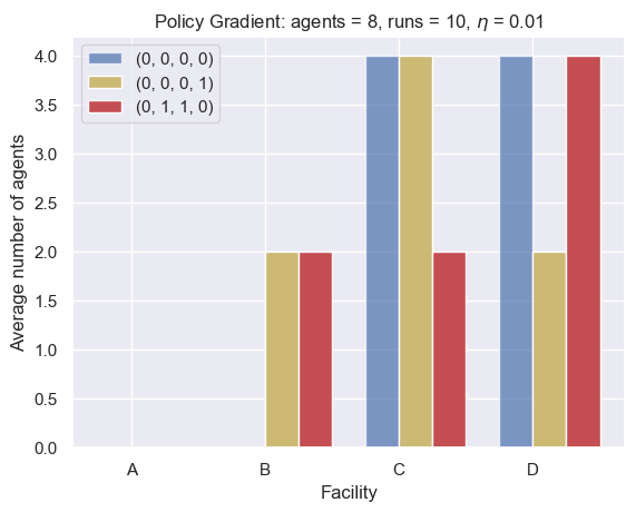
(a)

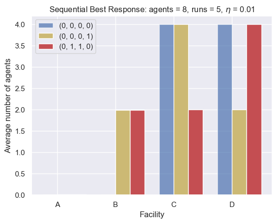
(b)

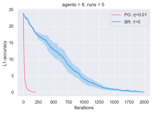
(c)

Figure 1: Markov congestion game: (a) and (b) are distributions of players taking four actions in representative states: (a) using Algorithm 1 with step-size $\eta=0.01$; (b) using Algorithm 2 with regularizer $\tau_{t}=0.999^{t}\cdot 5$. (c) is mean L1-accuracy with shaded region of one standard deviation over all runs.

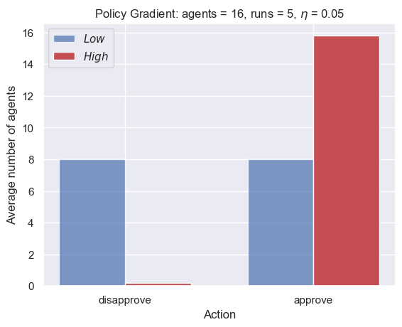
(a)

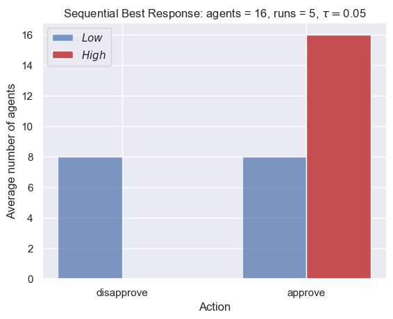
(b)

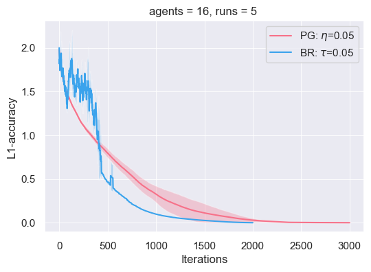
(c)

Figure 2: Perturbed Markov team game: (a) and (b) are distributions of players taking actions in all states: (a) using Algorithm 1 with step-size $\eta=0.05$; (b) using Algorithm 2 with regularizer $\tau_{t}=0.9975^{t}\cdot 0.05$. (c) is mean L1-accuracy with shaded region of one standard deviation over all runs.

6 Conclusion

This paper proposes a new notion of Markov $\alpha$-potential games to study multi-agent Markov games, along with an optimization-based approach to compute an upper bound of $\alpha$. This framework enables analyzing two practically significant classes of games. Our analysis shows that it is also a viable framework for studying the properties of MARL algorithms in general Markov games. Undoubtedly, there are a number of open questions in order for this framework to be further and fully developed. For instance, how to characterize explicitly the $\alpha$-potential function? How to design efficient algorithms to obtain tighter bounds of $\alpha$? And, how to establish last-iterate convergence guarantee of MARL algorithms under this framework?

7 Algorithms to solve (9)

In this section, we present an algorithm based on the stochastic gradient method from Tadić et al. [27] to solve the semi-infinite linear programming problem (9). Define

$$g(\phi;\pi,\pi^{\prime})=\max_{i\in I}\left|\sum_{s^{\prime},a^{\prime}}(d^{s}(s^{\prime},a^{\prime};\pi_{i},\pi_{-i})-d^{s}(s^{\prime},a^{\prime};\pi_{i}^{\prime},\pi_{-i}))(\phi-u_{i})(s^{\prime},a^{\prime})\right|,$$ (22)

with which the constraint (C1) in (9) can be rewritten as $g(\phi;\pi,\pi^{\prime})-y\leq 0,\forall\pi,\pi^{\prime}\in\Pi.$ Let $h:\mathbb{R}\rightarrow\mathbb{R}$ be a convex differentiable function such that

$$h(x)=0\text{ for all }x\leq 0,\text{ and }h(x)>0\text{ for all }x>0.$$

A candidate choice of $h$ is $h(x)=(\max\{0,x\})^{2}.$ Finally, we consider step-size schedules $\{\gamma_{t}\}_{t=1}^{\infty}$ and $\{\beta_{t}\}_{t=1}^{\infty}$ such that

$$\lim_{t\rightarrow\infty}\beta_{t}=\infty,\sum_{t=1}^{\infty}{\gamma_{t}^{2}\beta_{t}^{2}}<\infty,\sum_{t=1}^{\infty}\gamma_{t}=\infty,\text{ and }\gamma_{t}>0,\beta_{t}<\beta_{t+1}\text{ for all }t\geq 0.$$ (23)

Algorithm 1 Algorithm to solve (9) (Tadić et al. [27])

  Input: $y^{(0)}\in\mathbb{R}_{+},\phi^{(0)}\in\mathbb{R}^{S\times A}$, $\{\gamma_{t}\}_{t=1}^{\infty}$ and $\{\beta_{t}\}_{t=1}^{\infty}$ satisfying (23).

  for $t=0,1,2,...,T-1$ do

     Sample $\pi$, $\pi^{\prime}$ in $\Pi$ from uniform distribution and calculate $g(\phi^{(t)};\pi,\pi^{\prime})$ in (22).

     Update $\phi^{(t)}$ with

$$\phi^{(t+1)}=\phi^{(t)}-\gamma_{t+1}\beta_{t+1}h^{\prime}\left(g\left(\phi^{(t)};\pi,\pi^{\prime}\right)-y^{(t+1)}\right)\cdot\nabla_{\phi}g\left(\phi^{(t)};\pi,\pi^{\prime}\right),$$ (24)

and update $y^{(t)}$ with

$$y^{(t+1)}=y^{(t)}-\gamma_{t+1}+\gamma_{t+1}\beta_{t+1}h^{\prime}\left(g\left(\phi^{(t)};\pi,\pi^{\prime}\right)-y^{(t)}\right).$$

  end for

Theorem 4 in Tadić et al. [27] shows that with probability 1, $(y^{(t)},\phi^{(t)})$ almost surely converges to a solution of (9).

7.1 State-wise potential games

Algorithm 1 iteratively updates the variables $y\in\mathbb{R}$ and $\phi\in\mathbb{R}^{S\times A}$. However, this method may be slow as the dimension of $\phi$ scales exponentially with $|I|$. We show that for the class of games where each state is a static potential game, one can develop a faster algorithm than Algorithm 1. More formally, assume that there exists a function $\phi^{\ast}:S\times A\rightarrow\mathbb{R}$ such that for every $i\in I,s\in S,a_{i},a_{i}^{\prime}\in A_{i},a_{-i}\in A_{-i},$ $|\phi^{\ast}(s,a_{i},a_{-i})-\phi^{\ast}(s,a_{i}^{\prime},a_{-i})-(u_{i}(s,a_{i},a_{-i})-u_{i}(s,a_{i}^{\prime},a_{-i}))|=0.$ Note that Markov congestion games are a special case of such games. Now consider the following relaxation of (9),

$$\inf_{y\in\mathbb{R}}\quad\quad y$$ (25)

s.t. $$\left|\sum_{s^{\prime},a^{\prime}}(d^{s}(s^{\prime},a^{\prime};\pi_{i},\pi_{-i})-d^{s}(s^{\prime},a^{\prime};\pi_{i}^{\prime},\pi_{-i}))(\phi^{\ast}-u_{i})(s^{\prime},a^{\prime})\right|\leq y,$$

$$\quad~{}\forall s\in S,~{}\forall i\in I,~{}\forall\pi_{i},\pi^{\prime}_{i}\in{\Pi}_{i},~{}\forall\pi_{-i}\in{\Pi}_{-i}.$$

Note that (25) reduces the dimension of decision variables from $\mathcal{O}(|S|\cdot|A|)$ to $\mathcal{O}(1)$. In Algorithm 2 which solves (9) following Tadić et al. [27], only updating $y^{(t)}$ is necessary, as $\phi^{\ast}$ is pre-set to the static state potential function.

Algorithm 2 Algorithm to solve (25) (Tadić et al. [27])

  Input: $y^{(0)}\in\mathbb{R}_{+},\phi^{\ast}$, $\{\gamma_{t}\}_{t=1}^{\infty}$ and $\{\beta_{t}\}_{t=1}^{\infty}$ satisfying (23).

  for $t=0,1,2,...,T-1$ do

     Sample $\pi$, $\pi^{\prime}$ in $\Pi$ from uniform distribution and calculate $g(\phi^{\ast};\pi,\pi^{\prime})$ in (22).

     Update $y^{(t)}$ with

$$y^{(t+1)}=y^{(t)}-\gamma_{t+1}+\gamma_{t+1}\beta_{t+1}h^{\prime}\left(g\left(\phi^{\ast};\pi,\pi^{\prime}\right)-y^{(t)}\right).$$

  end for

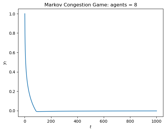
Figure 3: Find the closest Markov Potential Game to MCG using Algorithm 2. ($\gamma_{t}=\frac{1}{t},\beta_{t}=t^{0.4999},\,\forall t\geq 1.$)

Figure 3 shows the empirical performance of Algorithm 2 for the Markov congestion game. Note that with the setting in Section 5, $y^{(t)}$ converges to $0$ with Algorithm 2, which suggests that $\mathcal{G}_{\textsf{mcg}}$ may be an MPG, at least for some model parameters.

8 Proof of results in Section 3

Before presenting the proofs in this section we define some notations to simplify the exposition. Given a policy $(\pi_{i},\pi_{-i})\in\Pi$, and state $s,s^{\prime}\in S$, we define

$$P^{\pi}(s^{\prime}|s)=\sum_{a_{-i}\in A_{-i}}\pi_{-i}(a_{-i}|s)\sum_{a_{i}\in A_{i}}\pi_{i}(a_{i}|s)P(s^{\prime}|s,a).$$ (26)

8.1 Proof of Proposition 3.1

Before presenting the proof of Proposition 3.1, let us present a lemma that is crucial to the proof.

Lemma 8.1

If there exists some $\zeta>0$ such that for all $s,s^{\prime}\in S$, $|P(s^{\prime}|s,w)-P(s^{\prime}|s,w^{\prime})|\leq\zeta\|w-w^{\prime}\|_{1}$. Then for any $i\in I,\pi_{i},\pi_{i}^{\prime}\in\Pi_{i},\pi_{-i}\in\Pi_{-i}$,

$$\|P^{\pi_{i},\pi_{-i}}-P^{\pi_{i}^{\prime},\pi_{-i}}\|_{\infty}\leq\frac{2\zeta|S|\max_{a_{i}\in A_{i}}|a_{i}|}{|I|}.$$ (27)

Proof.

Proof.

For any $i\in I,\pi_{i},\pi_{i}^{\prime}\in\Pi_{i},\pi_{-i}\in\Pi_{-i}$, $s,s^{\prime}\in S$,

$$P^{\pi_{i},\pi_{-i}}(s^{\prime}|s)-P^{\pi_{i}^{\prime},\pi_{-i}}(s^{\prime}|s)$$

$$\stackrel{{\scriptstyle(a)}}{{=}}\sum_{a_{-i}\in A_{-i}}\pi_{-i}(s,a_{-i})\sum_{a_{i}\in A_{i}}\pi_{i}(s,a_{i})P(s^{\prime}|s,a_{i},a_{-i})-\sum_{a_{-i}\in A_{-i}}\pi_{-i}(s,a_{-i})\sum_{a_{i}\in A_{i}}\pi^{\prime}_{i}(s,a_{i})P(s^{\prime}|s,a_{i},a_{-i})$$

$$\stackrel{{\scriptstyle(b)}}{{=}}\sum_{a_{-i}\in A_{-i}}\pi_{-i}(s,a_{-i})\left(\sum_{a_{i}\in A_{i}}\pi_{i}(s,a_{i})P(s^{\prime}|s,w(a_{i},a_{-i}))-\sum_{a_{i}\in A_{i}}\pi^{\prime}_{i}(s,a_{i})P(s^{\prime}|s,w(a_{i},a_{-i}))\right)$$

$${\leq}\sum_{a_{-i}\in A_{-i}}\pi_{-i}(s,a_{-i})\left(\max_{a_{i}}P(s^{\prime}|s,w(a_{i},a_{-i}))-\min_{a_{i}}P(s^{\prime}|s,w(a_{i},a_{-i}))\right)$$

$${=}\sum_{a_{-i}\in A_{-i}}\pi_{-i}(s,a_{-i})\left(P(s^{\prime}|s,w(\bar{a}_{i},a_{-i}))-P(s^{\prime}|s,w(\underline{a}_{i},a_{-i}))\right),$$ (28)

where $\bar{a}_{i}\in\arg\max_{a_{i}\in A_{i}}P(s^{\prime}|s,w(a_{i},a_{-i}))$ and $\underline{a}_{i}\in\arg\min_{a_{i}\in A_{i}}P(s^{\prime}|s,w(a_{i},a_{-i}))$. Here, $(a)$ is due to (26), $(b)$ is due to the structure of congestion games (in Section 3), where the transition matrix only depends on action through aggregate usage vector $w$. By (8.1), for any $s\in S$,

$$\sum_{s^{\prime}\in S}|P^{\pi_{i},\pi_{-i}}(s^{\prime}|s)-P^{\pi_{i}^{\prime},\pi_{-i}}(s^{\prime}|s)|$$

$$\stackrel{{\scriptstyle(a)}}{{\leq}}\sum_{s^{\prime}\in S}\sum_{a_{-i}\in A_{-i}}\pi_{-i}(s,a_{-i})|P(s^{\prime}|s,w(\bar{a}_{i},a_{-i}))-P(s^{\prime}|s,w(\underline{a}_{i},a_{-i}))|$$

$$=\sum_{a_{-i}\in A_{-i}}\pi_{-i}(s,a_{-i})\sum_{s^{\prime}\in S}|P(s^{\prime}|s,w(\bar{a}_{i},a_{-i}))-P(s^{\prime}|s,w(\underline{a}_{i},a_{-i}))|$$

$$\stackrel{{\scriptstyle(b)}}{{\leq}}\zeta|S|\sum_{a_{-i}\in A_{-i}}\pi_{-i}(s,a_{-i})\|w(\bar{a}_{i},a_{-i})-w(\underline{a}_{i},a_{-i})\|_{1}$$

$$=\zeta|S|\sum_{a_{-i}\in A_{-i}}\pi_{-i}(s,a_{-i})\sum_{e\in E}|w_{e}(\bar{a}_{i},a_{-i})-w_{e}(\underline{a}_{i},a_{-i})|$$

$$\stackrel{{\scriptstyle(c)}}{{=}}\frac{\zeta|S|}{|I|}\sum_{a_{-i}\in A_{-i}}\pi_{-i}(s,a_{-i})\sum_{e\in E}|\mathbbm{1}(e\in\bar{a}_{i})-\mathbbm{1}(e\in\underline{a}_{i})|=\frac{2\zeta|S|\max_{a_{i}\in A_{i}}|a_{i}|}{|I|},$$

where $(a)$ is due to (8.1) and the triangle inequality, $(b)$ is due to the Lipschitz property of transition assumed in the statement of Lemma 8.1 and $(c)$ is by the definition of aggregate usage vector in (4). ∎

Proof.

Proof of Proposition 3.1.

Recall that for any $s\in S$, the stage game is a potential game with a potential function $\varphi(s,a)=1/|I|\sum_{e\in E}\sum_{j=1}^{w_{e}(a)|I|}c_{e}\left(s,j/|I|\right)$. That is, for any $s\in S,i\in I,a_{i},a_{i}^{\prime}\in A_{i},a_{-i}\in A_{-i}$,

$$\varphi(s,a_{i},a_{-i})-\varphi(s,a_{i}^{\prime},a_{-i})=u_{i}(s,a_{i},a_{-i})-u_{i}(s,a_{i}^{\prime},a_{-i}).$$ (29)

Under this notation, we can equivalently write (5) as

$$\Psi(s,\pi)=\mathbb{E}_{\pi}\Big{[}\sum_{k=0}^{\infty}\delta^{k}\varphi(s^{k},a^{k})\Big{|}s_{0}=s\Big{]}=\varphi(s,\pi)+\delta\sum_{s^{\prime}\in S}P(s^{\prime}|s,\pi)\Psi(s^{\prime},\pi).$$ (30)

For the rest of the proof we fix arbitrary $\pi_{i},\pi_{i}^{\prime}\in\Pi_{i},\pi_{-i}\in\Pi_{-i}$ and define $\pi=(\pi_{i},\pi_{-i}),\pi^{\prime}=(\pi_{i}^{\prime},\pi_{-i})$. Using (30), the difference of using two policies $\pi$ and $\pi^{\prime}$ can be written as

$$\Psi(s,\pi)-\Psi(s,\pi^{\prime})=\varphi(s,\pi)-\varphi(s,\pi^{\prime})+\delta\sum_{s^{\prime}\in S}\left(P(s^{\prime}|s,\pi)\Psi(s^{\prime},\pi)-P(s^{\prime}|s,\pi^{\prime})\Psi(s^{\prime},\pi^{\prime})\right).$$ (31)

Additionally, recall that the value function of player $i\in I$ with policy $\pi\in\Pi$ starting from state $s\in S$ is given by

$$V_{i}(s,\pi) =u_{i}(s,\pi)+\delta\sum_{s^{\prime}\in S}P(s^{\prime}|s,\pi)V_{i}(s^{\prime},\pi).$$ (32)

Consequently, the difference of the value functions of player $i$ evaluated at the policies $\pi$ and $\pi^{\prime}$ is given by

$$V_{i}(s,\pi)-V_{i}(s,\pi^{\prime})=u_{i}(s,\pi)-u_{i}(s,\pi^{\prime})+\delta\sum_{s^{\prime}\in S}\left(P(s^{\prime}|s,\pi)V_{i}(s^{\prime},\pi)-P(s^{\prime}|s,\pi^{\prime})V_{i}(s^{\prime},\pi^{\prime})\right).$$ (33)

Subtracting (31) from (33), clearly for any $s\in S$,

$$\left(V_{i}(s,\pi)-V_{i}(s,\pi^{\prime})\right)-\left(\Psi(s,\pi)-\Psi(s,\pi^{\prime})\right)$$

$${=}\left(u_{i}(s,\pi)-u_{i}(s,\pi^{\prime})\right)-\left(\varphi(s,\pi)-\varphi(s,\pi^{\prime})\right)$$

$$\quad+\delta\sum_{s^{\prime}\in S}P(s^{\prime}|s,\pi)\left(V_{i}(s^{\prime},\pi)-\Psi(s^{\prime},\pi)\right)-\sum_{s^{\prime}\in S}P(s^{\prime}|s,\pi^{\prime})\left(V_{i}(s^{\prime},\pi^{\prime})-\Psi(s^{\prime},\pi^{\prime})\right)$$

$$\stackrel{{\scriptstyle(a)}}{{=}}\delta\sum_{s^{\prime}\in S}P(s^{\prime}|s,\pi)\left(V_{i}(s^{\prime},\pi)-\Psi(s^{\prime},\pi)\right)-\sum_{s^{\prime}\in S}P(s^{\prime}|s,\pi^{\prime})\left(V_{i}(s^{\prime},\pi^{\prime})-\Psi(s^{\prime},\pi^{\prime})\right)$$

$$\stackrel{{\scriptstyle(b)}}{{=}}\delta\sum_{s^{\prime}\in S}P(s^{\prime}|s,\pi)\left(V_{i}(s^{\prime},\pi)-V_{i}(s^{\prime},\pi^{\prime})+\Psi(s^{\prime},\pi^{\prime})-\Psi(s^{\prime},\pi)\right)$$

$$\quad-\sum_{s^{\prime}\in S}\left(P(s^{\prime}|s,\pi^{\prime})-P(s^{\prime}|s,\pi)\right)\left(V_{i}(s^{\prime},\pi^{\prime})-\Psi(s^{\prime},\pi^{\prime})\right),$$

where $(a)$ is due to (29), $(b)$ is by adding and subtracting the term $\sum_{s^{\prime}\in S}P(s^{\prime}|s,\pi)(V_{i}(s^{\prime},\pi^{\prime})-\Psi(s^{\prime},\pi^{\prime})).$ Thus, it follows that

$$\max_{s\in S}|V_{i}(s,\pi)-V_{i}(s,\pi^{\prime})-\left(\Psi(s,\pi)-\Psi(s,\pi^{\prime})\right)|$$

$$\leq\delta\max_{s\in S}|V_{i}(s,\pi)-V_{i}(s,\pi^{\prime})-\left(\Psi(s,\pi)-\Psi(s,\pi^{\prime})\right)|$$

$$\quad\quad+\delta\max_{s\in S}\left|\sum_{s^{\prime}\in S}\left(\left(P(s^{\prime}|s,\pi)-P(s^{\prime}|s,\pi^{\prime})\right)\left(\Psi(s^{\prime},\pi)-V_{i}(s^{\prime},\pi)\right)\right)\right|$$

$$\leq\delta\max_{s\in S}|V_{i}(s,\pi)-V_{i}(s,\pi^{\prime})-\left(\Psi(s,\pi)-\Psi(s,\pi^{\prime})\right)|$$

$$\quad\quad+\delta\max_{s^{\prime}\in S}|\Psi(s^{\prime},\pi)-V_{i}(s^{\prime},\pi)|\max_{s\in S}\sum_{s^{\prime}\in S}\left|P(s^{\prime}|s,\pi)-P(s^{\prime}|s,\pi^{\prime})\right|.$$

Rearranging terms leads to

$$\max_{s\in S}|V_{i}(s,\pi)-V_{i}(s,\pi^{\prime})-\left(\Psi(s,\pi)-\Psi(s,\pi^{\prime})\right)|$$

$$\leq\frac{\delta}{1-\delta}\max_{s^{\prime}\in S}|\Psi(s^{\prime},\pi)-V_{i}(s^{\prime},\pi)|\max_{s\in S}\sum_{s^{\prime}\in S}\left|P(s^{\prime}|s,\pi)-P(s^{\prime}|s,\pi^{\prime})\right|$$

$$=\frac{\delta}{1-\delta}\max_{s^{\prime}\in S}|\Psi(s^{\prime},\pi)-V_{i}(s^{\prime},\pi)|\|P^{\pi}-P^{\pi^{\prime}}\|_{\infty}.$$ (34)

Using Lemma 8.1, one can bound (8.1) as follows

$$\max_{s\in S}|V_{i}(s,\pi)-V_{i}(s,\pi^{\prime})-\left(\Psi(s,\pi)-\Psi(s,\pi^{\prime})\right)|\leq\frac{2\delta\zeta|S|\max_{a_{i}\in A_{i}}|a_{i}|}{(1-\delta)|I|}\max_{s^{\prime}\in S}|\Psi(s^{\prime},\pi)-V_{i}(s^{\prime},\pi)|.$$

The claim follows by noting that for and $s^{\prime}\in S$,

$$|\Psi(s^{\prime},\pi)-V_{i}(s^{\prime},\pi)| =\left|\mathbb{E}\left[\sum_{k=0}^{\infty}\delta^{k}\sum_{e\in E}\left(\varphi(s^{k},a^{k})-u_{i}(s^{k},a^{k})\right)\right]\right|$$

$$\stackrel{{\scriptstyle(a)}}{{\leq}}\left|\mathbb{E}\left[\sum_{k=0}^{\infty}\delta^{k}\varphi(s^{k},a^{k})\right]\right|\leq\sup_{s,\pi}\Psi(s,\pi),$$

where $(a)$ holds because $u_{i}(s^{k},a^{k})={\sum_{e\in E}c_{e}(s^{k},w_{e}^{k})\mathbbm{1}(e\in a_{i}^{k})}\leq\sum_{e\in E}c_{e}(s^{k},w_{e}^{k})\leq\varphi(s^{k},a^{k}).$ ∎

8.2 Proof of Proposition 3.2

The goal is to show that for every $i\in I,\pi_{i},\pi_{i}^{\prime}\in\Pi_{i},\pi_{-i}\in\Pi_{-i}$, $\max_{s\in S}|V_{i}(s,\pi_{i},\pi_{-i})-V_{i}(s,\pi^{\prime}_{i},\pi_{-i})-\left(\Psi(s,\pi_{i},\pi_{-i})-\Psi(s,\pi^{\prime}_{i},\pi_{-i})\right)|\leq\frac{2\kappa}{(1-\delta)^{2}},$ where

$$\Psi(s,\pi)=\mathbb{E}_{\pi}\left[\sum_{k=0}^{\infty}\delta^{k}r(s^{k},a^{k})|s^{0}=s\right]=r(s,\pi)+\delta\sum_{s^{\prime}\in S}P(s^{\prime}|s,\pi)\Psi(s^{\prime},\pi).$$ (35)

Throughout the proof, let us fix arbitrary $\pi_{i},\pi_{i}^{\prime}\in\Pi_{i},\pi_{-i}\in\Pi_{-i}$, and define $\pi=(\pi_{i},\pi_{-i}),\pi^{\prime}=(\pi_{i}^{\prime},\pi_{-i})$. By (35), for any $s\in S$, the difference of $\Psi$ at two policies $\pi$ and $\pi^{\prime}$ is

$$\Psi(s,\pi)-\Psi(s,\pi^{\prime})=r(s,\pi)-r(s,\pi^{\prime})+\delta\sum_{s^{\prime}\in S}\left(P(s^{\prime}|s,\pi)\Psi(s^{\prime},\pi)-P(s^{\prime}|s,\pi^{\prime})\Psi(s^{\prime},\pi^{\prime})\right).$$ (36)

Similarly, for any $s\in S$, the difference in value function of player $i$ at $\pi,\pi^{\prime}$ is

$$V_{i}(s,\pi)-V_{i}(s,\pi^{\prime})=u_{i}(s,\pi)-u_{i}(s,\pi^{\prime})+\delta\sum_{s^{\prime}\in S}P(s^{\prime}|s,\pi)V_{i}(s^{\prime},\pi)-P(s^{\prime}|s,\pi^{\prime})V_{i}(s^{\prime},\pi^{\prime}).$$ (37)

Subtracting (LABEL:eq:_PotentialDiffPTMG) from (LABEL:eq:_ValueDiffPTMG), we observe that for any $s\in S$,

$$V_{i}(s,\pi)-V_{i}(s,\pi^{\prime})-\left(\Psi(s,\pi)-\Psi(s,\pi^{\prime})\right)$$

$${=}u_{i}(s,\pi)-u_{i}(s,\pi^{\prime})-\left(r(s,\pi)-r(s,\pi^{\prime})\right)-\delta\sum_{s^{\prime}\in S}P(s^{\prime}|s,\pi^{\prime})\left(V_{i}(s^{\prime},\pi^{\prime})-\Psi(s^{\prime},\pi^{\prime})\right)$$

$$\quad+\delta\sum_{s^{\prime}\in S}P(s^{\prime}|s,\pi)\left(V_{i}(s^{\prime},\pi)-\Psi(s^{\prime},\pi)\right)$$

$$\stackrel{{\scriptstyle(a)}}{{=}}u_{i}(s,\pi)-u_{i}(s,\pi^{\prime})-\left(r(s,\pi)-r(s,\pi^{\prime})\right)-\delta\sum_{s^{\prime}\in S}\left(P(s^{\prime}|s,\pi^{\prime})-P(s^{\prime}|s,\pi)\right)\left(V_{i}(s^{\prime},\pi^{\prime})-\Psi(s^{\prime},\pi^{\prime})\right)$$

$$\quad+\delta\sum_{s^{\prime}\in S}P(s^{\prime}|s,\pi)\left(V_{i}(s^{\prime},\pi)-V_{i}(s^{\prime},\pi^{\prime})+\Psi(s^{\prime},\pi^{\prime})-\Psi(s^{\prime},\pi)\right),$$

where $(a)$ is by adding and subtracting the term $\sum_{s^{\prime}\in S}P(s^{\prime}|s,\pi)\left(V_{i}(s^{\prime},\pi^{\prime})-\Psi(s^{\prime},\pi^{\prime})\right).$ Consequently,

$$\max_{s\in S}|V_{i}(s,\pi)-V_{i}(s,\pi^{\prime})-\left(\Psi(s,\pi)-\Psi(s,\pi^{\prime})\right)|$$

$$\leq\max_{s\in S}|\left(u_{i}(s,\pi)-u_{i}(s,\pi^{\prime})\right)-\left(r(s,\pi)-r(s,\pi^{\prime})\right)|$$

$$\quad+\delta\max_{s\in S}|V_{i}(s,\pi)-V_{i}(s,\pi^{\prime})-\left(\Psi(s,\pi)-\Psi(s,\pi^{\prime})\right)|$$

$$\quad+\delta\max_{s\in S}\left|\sum_{s^{\prime}\in S}\left(\left(P(s^{\prime}|s,\pi)-P(s^{\prime}|s,\pi^{\prime})\right)\left(\Psi(s^{\prime},\pi)-V_{i}(s^{\prime},\pi)\right)\right)\right|$$

$$\stackrel{{\scriptstyle(a)}}{{\leq}}2\kappa+\delta\max_{s\in S}|V_{i}(s,\pi)-V_{i}(s,\pi^{\prime})-\left(\Psi(s,\pi)-\Psi(s,\pi^{\prime})\right)|$$

$$\quad\quad+\delta\max_{s^{\prime}\in S}|\Psi(s^{\prime},\pi)-V_{i}(s^{\prime},\pi)|\max_{s\in S}\sum_{s^{\prime}\in S}\left|P(s^{\prime}|s,\pi)-P(s^{\prime}|s,\pi^{\prime})\right|,$$ (38)

where $(a)$ is due to the fact $|\left(u_{i}(s,\pi)-u_{i}(s,\pi^{\prime})\right)-\left(r(s,\pi)-r(s,\pi^{\prime})\right)|\leq 2\max_{\pi\in\Pi}|u_{i}(s,\pi)-r(s,\pi)|\leq 2\max_{s\in S,\pi\in\Pi}|\xi_{i}(s,\pi)|\leq 2\kappa.$ Rearranging terms in (8.2), we obtain

$$\max_{s\in S}|V_{i}(s,\pi)-V_{i}(s,\pi^{\prime})-\left(\Psi(s,\pi)-\Psi(s,\pi^{\prime})\right)|$$

$$\leq\frac{2\kappa}{1-\delta}+\frac{\delta}{1-\delta}\max_{s^{\prime}\in S}|\Psi(s^{\prime},\pi)-V_{i}(s^{\prime},\pi)|\max_{s\in S}\sum_{s^{\prime}\in S}\left|P(s^{\prime}|s,\pi)-P(s^{\prime}|s,\pi^{\prime})\right|$$

$$=\frac{2\kappa}{1-\delta}+\frac{2\delta}{1-\delta}\max_{s^{\prime}\in S}|\Psi(s^{\prime},\pi)-V_{i}(s^{\prime},\pi)|.$$ (39)

Finally, note that

$$|\Psi(s^{\prime},\pi)-V_{i}(s^{\prime},\pi)|=\left|\sum_{k=0}^{\infty}\delta^{k}\xi_{i}(s,\pi(s^{k}))\right|\leq\frac{\kappa}{1-\delta}.$$ (40)

Combining (8.2) and (40), we conclude that

$$\max_{s\in S}|V_{i}(s,\pi)-V_{i}(s,\pi^{\prime})-\left(\Psi(s,\pi)-\Psi(s,\pi^{\prime})\right)|\leq\frac{2\kappa}{1-\delta}+\frac{2\delta\kappa}{(1-\delta)^{2}}=\frac{2\kappa}{(1-\delta)^{2}}.$$

8.3 Proof of Proposition 3.3

Fix $\epsilon>0.$ Let $\pi^{*}=(\pi_{i}^{*},\pi_{-i}^{*})$ be such that

$$\Phi(s,\pi^{*})+\epsilon\geq\sup_{\pi\in\Pi}\Phi(s,\pi),\quad\text{for every}\ s\in S.$$ (41)

Then for every $s\in S$, $i\in I,\pi_{i}\in\Pi_{i}$, $V_{i}(s,\pi^{\ast})-V_{i}(s,\pi_{i},\pi_{-i}^{\ast})\stackrel{{\scriptstyle(a)}}{{\geq}}\Phi(s,\pi^{\ast})-\Phi(s,\pi_{i},\pi_{-i}^{\ast})-\alpha\stackrel{{\scriptstyle(b)}}{{\geq}}-\epsilon-\alpha,$ where $(a)$ is due to (3) and $(b)$ is due to (41). Thus, by Definition 3.4, $\pi^{*}$ is an $(\epsilon+\alpha)$-NE policy.

9 Proof of results in Section 4

9.1 Proof of Theorem 4.1

Lemma 9.1 (Performance difference)

For the $i$th player, if we fix the policy $\pi_{-i}$ and any state distribution $\mu$, then for any two policies ${\pi}^{\prime}_{i}$ and ${\pi}_{i}$,

$$V_{i}(\mu,{{\pi}^{\prime}_{i},\pi_{-i}})-V_{i}(\mu,{{\pi}_{i},\pi_{-i}})=\frac{1}{1-\delta}\sum_{s,a_{i}}d_{\mu}^{{\pi}^{\prime}_{i},\pi_{-i}}(s)\cdot\left({\pi}^{\prime}_{i}(s,a_{i})-{\pi}_{i}(s,a_{i})\right){Q}_{i}\left(s,a_{i};{{\pi}_{i},\pi_{-i}}\right).$$

Proof.

Proof. This lemma follows from a direct application of the performance difference lemma in Agarwal et al. [1]. ∎

We now introduce some notations adopted from Ding et al. [11] that will be used throughout the section: for $i,j\in\{1,...,|I|\}$ with $i<j$, denote by “$i\sim j$” the set of indices $\{k\mid i<k<j\},``<i$” the set of indices $\{k\mid k=1,\ldots,i-1\}$, and “$>j$” the set of indices $\{k\mid k=j+1,\ldots,|I|\}$. We use the shorthand $\pi_{I}:=\left\{\pi_{k}\right\}_{k\in I}$ to represent the joint policy for all players $k\in I$. For example, when $I=i\sim j,\pi_{I}=\left\{\pi_{k}\right\}_{k=i+1}^{j-1}$ is a joint policy for players from $i+1$ to $j-1;\pi_{<i,i\sim j},\pi_{<i}$, and $\pi_{>j}$ can be introduced similarly.

Lemma 9.2 (Lemma 2 in Ding et al. [11])

For any function $f^{\pi}:\Pi\rightarrow\mathbb{R}$, and any two policies $\pi,\pi^{\prime}\in\Pi$,

$$f^{\pi^{\prime}}-f^{\pi}=\sum_{i=1}^{|I|}\left(f^{\pi_{i}^{\prime},\pi_{-i}}-f^{\pi}\right)$$

$$\quad\quad+\sum_{i=1}^{|I|}\sum_{j=i+1}^{|I|}\left(f^{\pi_{<i,i\sim j},\pi_{>j}^{\prime},\pi_{i}^{\prime},\pi_{j}^{\prime}}-f^{\pi_{<i,i\sim j},\pi_{>j}^{\prime},\pi_{i},\pi_{j}^{\prime}}-f^{\pi_{<i,i\sim j},\pi_{>j}^{\prime},\pi_{i}^{\prime},\pi_{j}}+f^{\pi_{<i,i\sim j},\pi_{>j}^{\prime},\pi_{i},\pi_{j}}\right).$$

Lemma 9.3 ( Lemma 21 in Ding et al. [11])

Consider a two-player common-payoff Markov game with state space $S$ and action sets $A_{1},A_{2}$. Let $u:{S}\times{A}_{1}\times{A}_{2}\rightarrow[0,1]$ be the utility function, and $p:{S}\times{A}_{1}\times{A}_{2}\rightarrow\Delta({S})$ be the transition function. Let $\Pi_{1}=\left(\Delta\left({A}_{1}\right)\right)^{{|S|}}$ and $\Pi_{2}=\left(\Delta\left({A}_{2}\right)\right)^{{|S|}}$ be player 1 and player 2’s policy sets, respectively. Then, for any $x,x^{\prime}\in\Pi_{1}$ and $y,y^{\prime}\in\Pi_{2}$,

$$V(\mu,x,y)-V(\mu,x^{\prime},y)-V(\mu,x,y^{\prime})+V(\mu,x^{\prime},y^{\prime})$$

$$\leq\frac{2\kappa_{\mu}^{2}\bar{A}}{(1-\delta)^{4}}\sum_{s}d_{\mu}^{x^{\prime},y^{\prime}}(s)\left(\left\|x(\cdot\mid s)-x^{\prime}(\cdot\mid s)\right\|^{2}+\left\|y(\cdot\mid s)-y^{\prime}(\cdot\mid s)\right\|^{2}\right),$$

with $\kappa_{\mu}$ defined in (1).

Lemma 9.4 (Policy improvement)

For Markov $\alpha$-potential game (3.2) with any state distribution $\nu$, the $\alpha$-potential function $\Phi(\nu,\pi)$ at two consecutive policies $\pi^{(t+1)}$ and $\pi^{(t)}$ in Algorithm 1 satisfies

$$(i)\,\Phi(\nu,{\pi^{(t+1)}})-\Phi(\nu,{\pi^{(t)}})\geq -\frac{4\eta^{2}\bar{A}^{2}|I|^{2}}{(1-\delta)^{5}}-|I|^{2}\alpha$$

$$+\frac{1}{2\eta(1-\delta)}\sum_{i\in I,s\in S}d_{\nu}^{\pi_{i}^{(t+1)},\pi_{-i}^{(t)}(s)}\left\|\pi_{i}^{(t+1)}(s)-\pi_{i}^{(t)}(s)\right\|^{2};$$

$$(ii) \Phi(\nu,{\pi^{(t+1)}})-\Phi(\nu,{\pi^{(t)}})\geq-|I|^{2}\alpha$$

$$\quad\quad\quad\quad+\frac{1}{2\eta(1-\delta)}\left(1-\frac{4\eta\kappa_{\nu}^{3}\bar{A}|I|}{(1-\delta)^{4}}\right)\sum_{i=1}^{|I|}\sum_{s}d_{\nu}^{\pi_{i}^{(t+1)},\pi_{-i}^{(t)}(s)}\left\|\pi_{i}^{(t+1)}(\cdot\mid s)-\pi_{i}^{(t)}(\cdot\mid s)\right\|^{2}.$$

Proof.

Proof. Fix $\nu\in\Delta(S)$. For ease of exposition, let $\pi^{\prime}=\pi^{(t+1)}$ and $\pi=\pi^{(t)}$. By Lemma 9.2 with $f^{\pi}=\Phi(\nu,\pi)$, it is equivalent to analyzing

$$\Phi(\nu,{\pi^{(t+1)}})-\Phi(\nu,{\pi^{(t)}})=\operatorname{Diff}_{a}+\operatorname{Diff}_{b},$$ (42)

where

$$\operatorname{Diff}_{a}=\sum_{i=1}^{|I|}\Phi(\nu,{\pi_{i}^{\prime},\pi_{-i}})-\Phi(\nu,\pi),$$ (43)

$$\operatorname{Diff}_{b}=\sum_{i=1}^{|I|}\sum_{j=i+1}^{|I|} \left(\Phi(\nu,{\pi_{<i,i\sim j},\pi_{>j}^{\prime},\pi_{i}^{\prime},\pi_{j}^{\prime}})-\Phi(\nu,{\pi_{<i,i\sim j},\pi_{>j}^{\prime},\pi_{i},\pi_{j}^{\prime}})\right.$$

$$\left.-\Phi(\nu,{\pi_{<i,i\sim j},\pi_{>j}^{\prime},\pi_{i}^{\prime},\pi_{j}})+\Phi(\nu,{\pi_{<i,i\sim j},\pi_{>j}^{\prime},\pi_{i},\pi_{j}})\right).$$

Bounding Diff_a.

By the property of the $\alpha$-potential function $\Phi(\nu,\pi)$,

$$\Phi(\nu,{\pi_{i}^{\prime},\pi_{-i}})-\Phi(\nu,\pi)+\alpha \geq V_{i}(\nu,{\pi_{i}^{\prime},\pi_{-i}})-V_{i}(\nu,\pi)$$

$$=\frac{1}{1-\delta}\sum_{s,a_{i}}d_{\nu}^{\pi_{i}^{\prime},\pi_{-i}}(s)\left(\pi_{i}^{\prime}\left(s,a_{i}\right)-\pi_{i}\left(s,a_{i}\right)\right){Q}_{i}\left(s,a_{i};{\pi_{i},\pi_{-i}}\right),$$

where the equality follows from Lemma 9.1. The optimality of $\pi_{i}^{\prime}=\pi_{i}^{(t+1)}$ in (10) leads to

$$\left\langle\pi_{i}^{\prime}(s),{Q}_{i}(s;\pi_{i},\pi_{-i})\right\rangle_{{A}_{i}}-\frac{1}{2\eta}\left\|\pi_{i}^{\prime}(s)-\pi_{i}(s)\right\|^{2}\geq\left\langle\pi_{i}(s),{Q}_{i}(s;{\pi_{i},\pi_{-i}})\right\rangle_{{A}_{i}}.$$

Combining the above two parts yields

$$\Phi(\nu,{\pi_{i}^{\prime},\pi_{-i}})-\Phi(\nu,\pi)+\alpha\geq\frac{1}{2\eta(1-\delta)}\sum_{s}d_{\nu}^{\pi_{i}^{\prime},\pi_{-i}}(s)\left\|\pi_{i}^{\prime}(s)-\pi_{i}(s)\right\|^{2}.$$

By summing up $i$ from $1$ to $|I|$, we can get

$$\operatorname{Diff}_{a}\geq\frac{1}{2\eta(1-\delta)}\sum_{i=1}^{|I|}\sum_{s}d_{\nu}^{\pi_{i}^{(t+1)},\pi_{-i}^{(t)}}(s)\left\|\pi_{i}^{(t+1)}(s)-\pi_{i}^{(t)}(s)\right\|^{2}-|I|\alpha.$$ (44)

Bounding Diff_b.

There are two ways to bound $\text{Diff}_{b}$. (1) For any $\tilde{\pi}_{-ij},\pi^{\prime}_{i},\pi_{i},\pi^{\prime}_{j},\pi_{j}$,

$$\Phi(\nu,{\tilde{\pi}_{-ij},\pi_{i}^{\prime},\pi_{j}^{\prime}})-\Phi(\nu,{\tilde{\pi}_{-ij},\pi_{i},\pi_{j}^{\prime}})-\Phi(\nu,{\tilde{\pi}_{-ij},\pi_{i}^{\prime},\pi_{j}})+\Phi(\nu,{\tilde{\pi}_{-ij},\pi_{i},\pi_{j}})+2\alpha$$

$$\geq V_{i}(\nu,{\tilde{\pi}_{-ij},\pi_{i}^{\prime},\pi_{j}^{\prime}})-V_{i}(\nu,{\tilde{\pi}_{-ij},\pi_{i},\pi_{j}^{\prime}})-V_{i}(\nu,{\tilde{\pi}_{-ij},\pi_{i}^{\prime},\pi_{j}})+V_{i}(\nu,{\tilde{\pi}_{-ij},\pi_{i},\pi_{j}})\geq-\frac{8\eta^{2}\bar{A}^{2}}{(1-\delta)^{5}},$$

where the second inequality is from Lemma 3 in Ding et al. [11]. Thus,

$$\operatorname{Diff}_{b}\geq-\frac{|I|(|I|-1)}{2}\times\left(\frac{8\eta^{2}\bar{A}^{2}}{(1-\delta)^{5}}+2\alpha\right)\geq-\frac{4\eta^{2}\bar{A}^{2}|I|^{2}}{(1-\delta)^{5}}-|I|(|I|-1)\alpha.$$ (45)

Combining (42), (44) and (45) finishes the proof of (i).

(2) We can also bound each summand of $\text{Diff}_{b}$ by Lemma 9.3,

$$\Phi(\nu,{\tilde{\pi}_{-ij},\pi_{i}^{\prime},\pi_{j}^{\prime}})-\Phi(\nu,{\tilde{\pi}_{-ij},\pi_{i},\pi_{j}^{\prime}})-\Phi(\nu,{\tilde{\pi}_{-ij},\pi_{i}^{\prime},\pi_{j}})+\Phi(\nu,{\tilde{\pi}_{-ij},\pi_{i},\pi_{j}})+2\alpha$$

$$\geq V_{i}(\nu,{\tilde{\pi}_{-ij},\pi_{i}^{\prime},\pi_{j}^{\prime}})-V_{i}(\nu,{\tilde{\pi}_{-ij},\pi_{i},\pi_{j}^{\prime}})-V_{i}(\nu,{\tilde{\pi}_{-ij},\pi_{i}^{\prime},\pi_{j}})+V_{i}(\nu,{\tilde{\pi}_{-ij},\pi_{i},\pi_{j}})$$

$$\geq -\frac{2\kappa_{\nu}^{2}\bar{A}}{(1-\delta)^{4}}\sum_{s}d_{\nu}^{\tilde{\pi}_{-ij},\pi_{i},\pi_{j}}(s)\left(\left\|\pi_{i}(\cdot\mid s)-\pi_{i}^{\prime}(\cdot\mid s)\right\|^{2}+\left\|\pi_{j}(\cdot\mid s)-\pi_{j}^{\prime}(\cdot\mid s)\right\|^{2}\right).$$

Thus,

$$\operatorname{Diff}_{b}\geq-|I|(|I|-1)\alpha-\frac{2\kappa_{\nu}^{2}\bar{A}}{(1-\delta)^{4}}\sum_{i=1}^{N}\sum_{j=i+1}^{N}\sum_{s}d_{\nu}^{\tilde{\pi}_{-ij},\pi_{i},\pi_{j}}(s)\Big{(} \left\|\pi_{i}(\cdot\mid s)-\pi_{i}^{\prime}(\cdot\mid s)\right\|^{2}$$ (46)

$$+\left\|\pi_{j}(\cdot\mid s)-\pi_{j}^{\prime}(\cdot\mid s)\right\|^{2}\Big{)}.$$

Note that for any $\pi^{\prime},\nu,s$, it holds that

$$d_{\nu}^{\pi^{\prime}}(s)=(1-\delta)\mathbb{E}_{s_{0}\sim\nu}\left[\sum_{k=0}^{\infty}\delta^{k}P(s^{k}=s|s^{0})\right]\geq(1-\delta)\mathbb{E}_{s_{0}\sim\nu}\left[\delta^{0}P(s^{0}=s|s^{0})\right]=(1-\delta)\nu(s),$$

which immediately implies $\frac{d_{\nu}^{\pi}(s)}{d_{\nu}^{\pi^{\prime}}(s)}\leq\frac{\kappa_{\nu}}{1-\delta}$ for any $\pi,\pi^{\prime},\nu.$ Plug into (46) to get

$$\operatorname{Diff}_{b} \geq-|I|(|I|-1)\alpha-\frac{2\kappa_{\nu}^{3}|I|\bar{A}}{(1-\delta)^{5}}\sum_{i=1}^{|I|}\sum_{s}d_{\nu}^{\pi_{i}^{(t+1)},\pi_{-i}^{(t)}}(s)\left\|\pi_{i}^{(t)}(\cdot\mid s)-\pi_{i}^{(t+1)}(\cdot\mid s)\right\|^{2}.$$

Combine the inequality above with (42) and (44) to finish the proof of (ii). ∎

9.1.1 Proof of Theorem 4.1

Observe that the update in (10) can be equivalently described as

$$\pi_{i}^{(t+1)}(s)={\operatorname{argmax}}_{\pi_{i}(s)\in\Delta\left({A}_{i}\right)}\left\{\left\langle\pi_{i}(s),{Q}_{i}^{(t)}(s)\right\rangle_{{A}_{i}}-\frac{1}{2\eta}\left\|\pi_{i}(s)-\pi_{i}^{(t)}(s)\right\|^{2}\right\},\quad\forall\ s\in S.$$ (47)

This implies that for any $\pi_{i}^{\prime}\in\Pi_{i}$, $\left\langle\pi_{i}^{\prime}(s)-\pi_{i}^{(t+1)}(s),\eta{Q}_{i}^{(t)}(s)-\pi_{i}^{(t+1)}(s)+\pi_{i}^{(t)}(s)\right\rangle_{A_{i}}\leq 0.$ Hence, if $\eta\leq\frac{1-\delta}{\sqrt{\bar{A}}}$, then for any $\pi_{i}^{\prime}\in\Pi_{i}$,

$$\left\langle\pi_{i}^{\prime}(s)-\pi_{i}^{(t)}(s),{Q}_{i}^{(t)}(s)\right\rangle_{A_{i}}=\left\langle\pi_{i}^{\prime}(s)-\pi_{i}^{(t+1)}(s),{Q}_{i}^{(t)}(s)\right\rangle_{A_{i}}+\left\langle\pi_{i}^{(t+1)}(s)-\pi_{i}^{(t)}(s),{Q}_{i}^{(t)}(s)\right\rangle_{A_{i}}$$

$$\leq\frac{1}{\eta}\left\langle\pi_{i}^{\prime}(s)-\pi_{i}^{(t+1)}(s),\pi_{i}^{(t+1)}(s)-\pi_{i}^{(t)}(s)\right\rangle_{A_{i}}+\left\langle\pi_{i}^{(t+1)}(s)-\pi_{i}^{(t)}(s),{Q}_{i}^{(t)}(s)\right\rangle_{A_{i}}.$$

Note that for any two probability distributions $p_{1}$ and $p_{2}$, $\|p_{1}-p_{2}\|\leq\|p_{1}-p_{2}\|_{1}\leq 2.$ Therefore,

$$\left\langle\pi_{i}^{\prime}(s)-\pi_{i}^{(t)}(s),{Q}_{i}^{(t)}(s)\right\rangle_{A_{i}}\leq\frac{2}{\eta}\left\|\pi_{i}^{(t+1)}(s)-\pi_{i}^{(t)}(s)\right\|+\left\|\pi_{i}^{(t+1)}(s)-\pi_{i}^{(t)}(s)\right\|\left\|{Q}_{i}^{(t)}(s)\right\|$$ (48)

$$\leq\frac{3}{\eta}\left\|\pi_{i}^{(t+1)}(s)-\pi_{i}^{(t)}(s)\right\|,$$

where the last inequality is due to $\left\|{Q}_{i}^{(t)}(s)\right\|\leq\frac{\sqrt{\bar{A}}}{1-\delta}\text{ and }\eta\leq\frac{1-\delta}{\sqrt{\bar{A}}}$. Hence, by Lemma 9.1 and (48),

$$T\cdot\text{Nash-regret}(T)=\sum_{t=1}^{T}\max_{i}\left(\max_{\pi_{i}^{\prime}}V_{i}(\mu,{\pi_{i}^{\prime},\pi_{-i}^{(t)}})-V_{i}(\mu,{\pi^{(t)}})\right)$$

$$\overset{(a)}{=}\frac{1}{1-\delta}\sum_{t=1}^{T}\max_{\pi_{i}^{\prime}}\sum_{s,a_{i}}d_{\mu}^{\pi_{i}^{\prime},\pi_{-i}^{(t)}}(s)\left(\pi_{i}^{\prime}\left(s,a_{i}\right)-\pi_{i}^{(t)}\left(s,a_{i}\right)\right){Q}_{i}^{(t)}\left(s,a_{i}\right)$$

$$\overset{(b)}{\leq}\frac{3}{\eta(1-\delta)}\sum_{t=1}^{T}\sum_{s}d_{\mu}^{\pi_{i}^{\prime},\pi_{-i}^{(t)}}(s)\left\|\pi_{i}^{(t+1)}(s)-\pi_{i}^{(t)}(s)\right\|,$$

where in the equality $(a)$ we slightly abuse the notation $i$ to represent $\arg\max_{i}$ and in $(b)$ we slightly abuse the notation $\pi_{i}^{\prime}$ to represent $\arg\max_{\pi_{i}^{\prime}}.$ Now, continuing the above calculation with an arbitrary $\nu\in\Delta({S})$ and using the following inequality

$$\frac{d_{\mu}^{\pi_{i}^{\prime},\pi_{-i}^{(t)}}(s)}{d_{\nu}^{\pi_{i}^{(t+1)},\pi_{-i}^{(t)}}(s)}\leq\frac{d_{\mu}^{\pi_{i}^{\prime},\pi_{-i}^{(t)}}(s)}{(1-\delta)\nu(s)}\leq\frac{\sup_{\pi\in\Pi}\left\|d_{\mu}^{\pi}/\nu\right\|_{\infty}}{1-\delta},$$

to get:

$$T\cdot\text{Nash-regret}(T)$$

$${\leq}\frac{3\sqrt{\sup_{\pi\in\Pi}\left\|d_{\mu}^{\pi}/\nu\right\|_{\infty}}}{\eta(1-\delta)^{\frac{3}{2}}}\sum_{t=1}^{T}\sum_{s}\sqrt{d_{\mu}^{\pi_{i}^{\prime},\pi_{-i}^{(t)}}(s)d_{\nu}^{\pi_{i}^{(t+1)},\pi_{-i}^{(t)}}(s)}\left\|\pi_{i}^{(t+1)}(s)-\pi_{i}^{(t)}(s)\right\|$$

$$\overset{(c)}{\leq}\frac{3\sqrt{\sup_{\pi\in\Pi}\left\|d_{\mu}^{\pi}/\nu\right\|_{\infty}}}{\eta(1-\delta)^{\frac{3}{2}}}\sqrt{\sum_{t=1}^{T}\sum_{s}d_{\mu}^{\pi_{i}^{\prime},\pi_{-i}^{(t)}}(s)}\sqrt{\sum_{t=1}^{T}\sum_{s}d_{\nu}^{\pi_{i}^{(t+1)},\pi_{-i}^{(t)}(s)}\left\|\pi_{i}^{(t+1)}(s)-\pi_{i}^{(t)}(s)\right\|^{2}}$$

$$\overset{(d)}{\leq}\frac{3\sqrt{\sup_{\pi\in\Pi}\left\|d_{\mu}^{\pi}/\nu\right\|_{\infty}}}{\eta(1-\delta)^{\frac{3}{2}}}\sqrt{\sum_{t=1}^{T}\sum_{s}d_{\mu}^{\pi_{i}^{\prime},\pi_{-i}^{(t)}}(s)}\sqrt{\sum_{t=1}^{T}\sum_{i=1}^{|I|}\sum_{s}d_{\nu}^{\pi_{i}^{(t+1)},\pi_{-i}^{(t)}(s)}\left\|\pi_{i}^{(t+1)}(s)-\pi_{i}^{(t)}(s)\right\|^{2}},$$

where $(c)$ follows from the Cauchy-Schwartz inequality and in $(d)$ we replace $i$ ($\arg\max_{i}$) by the sum over all players. There are two choices to proceed the above calculation: (1) Fix $\epsilon>0.$ Take $\nu^{*}_{\epsilon}\in\Delta(S)$ such that $\sup_{\pi\in\Pi}\left\|\frac{d_{\mu}^{\pi}}{\nu_{\epsilon}^{*}}\right\|_{\infty}-\epsilon\leq\inf_{\nu\in\Delta(S)}\sup_{\pi\in\Pi}\left\|\frac{d_{\mu}^{\pi}}{\nu_{\epsilon}^{*}}\right\|_{\infty}$. Then apply Lemma 9.4 (i) to get

$$T\cdot\text{Nash-regret}(T)$$

$$\leq\frac{3\sqrt{(\widetilde{\kappa}_{\mu}+\epsilon)}}{\eta(1-\delta)^{\frac{3}{2}}}\sqrt{T}\sqrt{2\eta(1-\delta)\left(\Phi(\nu^{*}_{\epsilon},{\pi^{(T)}})-\Phi(\nu^{*}_{\epsilon},{\pi^{(0)}})\right)+\frac{8\eta^{3}\bar{A}^{2}|I|^{2}}{(1-\delta)^{4}}T+2\eta(1-\delta)|I|^{2}\alpha\cdot T}$$

$$\leq\frac{3\sqrt{(\widetilde{\kappa}_{\mu}+\epsilon)}}{\eta(1-\delta)^{\frac{3}{2}}}\sqrt{T}\sqrt{2\eta(1-\delta)C_{\Phi}+\frac{8\eta^{3}\bar{A}^{2}|I|^{2}}{(1-\delta)^{4}}T+2\eta(1-\delta)|I|^{2}\alpha\cdot T}$$

$$=3\sqrt{\frac{2(\widetilde{\kappa}_{\mu}+\epsilon)T(C_{\Phi}+|I|^{2}\alpha\cdot T)}{\eta(1-\delta)^{2}}+\frac{8(\widetilde{\kappa}_{\mu}+\epsilon)\eta T^{2}\bar{A}^{2}|I|^{2}}{(1-\delta)^{7}}},$$

where the second inequality follows from $\|\Phi(\nu,\pi)-\Phi(\nu,{\pi^{\prime}})\|\leq C_{\Phi}$ for any $\pi,\pi^{\prime}\in\Pi,\nu\in\Delta(S)$. By letting $\epsilon$ goes to $0$ and taking step size $\eta=\frac{(1-\delta)^{2.5}\sqrt{C_{\Phi}+|I|^{2}\alpha T}}{2|I|\bar{A}\sqrt{T}}$, we can complete the proof with

$$\text{Nash-regret}(T)\leq\frac{3\cdot 2^{\frac{3}{2}}\sqrt{{\tilde{\kappa}_{\mu}}\bar{A}|I|}}{(1-\delta)^{\frac{9}{4}}}\left(\frac{C_{\Phi}}{T}+|I|^{2}\alpha\right)^{\frac{1}{4}}.$$

(2) we can also proceed the calculation with Lemma 9.4 (ii) and $\eta\leq\frac{(1-\delta)^{4}}{8\kappa_{\nu}^{3}|I|\bar{A}}$ to get

$$T\cdot\text{Nash-regret}(T) \leq\frac{3\sqrt{\sup_{\pi\in\Pi}\left\|d_{\mu}^{\pi}/\nu\right\|_{\infty}}}{\eta(1-\delta)^{\frac{3}{2}}}\sqrt{T}\sqrt{{4\eta(1-\delta)}\left(\Phi(\nu,{\pi^{(T+1)}})-\Phi(\nu,{\pi^{(1)}})+|I|^{2}\alpha\cdot T\right)}$$

$$=6\sqrt{\frac{\sup_{\pi\in\Pi}\left\|d_{\mu}^{\pi}/\nu\right\|_{\infty}T(C_{\Phi}+|I|^{2}\alpha\cdot T)}{\eta(1-\delta)^{2}}}.$$

We next discuss two special choices of $\nu$ for proving our bound. First, if $\nu=\mu$, then $\eta\leq\frac{(1-\delta)^{4}}{8\kappa_{\mu}^{3}|I|\bar{A}}$. By letting $\eta=\frac{(1-\delta)^{4}}{8\kappa_{\mu}^{3}|I|\bar{A}}$, the last square root term can be bounded by $\mathcal{O}\Bigg{(}\sqrt{\frac{\kappa_{\mu}^{4}|I|\bar{A}T(C_{\Phi}+|I|^{2}\alpha\cdot T)}{(1-\delta)^{6}}}\Bigg{)}.$ Second, if $\nu=\frac{1}{|S|}\mathbf{1}$, the uniform distribution over ${S}$, then $\kappa_{\nu}\leq\frac{1}{S}$, which allows a valid choice $\eta=\frac{(1-\delta)^{4}}{8|S|^{3}|I|\bar{A}}\leq\frac{(1-\delta)^{4}}{8\kappa_{\nu}^{3}|I|\bar{A}}$. Hence, we can bound the last square root term by $\mathcal{O}\left(\sqrt{\frac{|S|^{4}|I|\bar{A}T(C_{\Phi}+|I|^{2}\alpha\cdot T)}{(1-\delta)^{6}}}\right).$ Since $\nu$ is arbitrary, combining these two special choices completes the proof.

9.2 Proof of Theorem 4.2

The proof of Theorem 4.2 needs the following technical lemmas.

9.2.1 Technical Lemmas

Lemma 9.5

If $\mathcal{G}$ is a Markov $\alpha$-potential game with $\Phi$ as its $\alpha$-potential function, then for any $s\in S,i\in I,\pi_{i}^{\prime},\pi_{i}\in\Pi_{i},\pi_{-i}\in\Pi_{-i}$,

$$\bigg{|}\left(\tilde{\Psi}\left(s,\pi_{i}^{\prime},\pi_{-i}\right)-\tilde{\Psi}\left(s,\pi_{i},\pi_{-i}\right)\right)-\left(\tilde{V}_{i}\left(s,\pi_{i}^{\prime},\pi_{-i}\right)-\tilde{V}_{i}\left(s,\pi_{i},\pi_{-i}\right)\right)\bigg{|}\leq\alpha,$$

where $\tilde{\Psi}(s,\pi):=\Phi(s,\pi)-\tau\mathbb{E}_{\pi}\left[\sum_{j\in I}\sum_{k=0}^{\infty}\delta^{k}\nu_{j}(s^{k},\pi_{j})\mid s^{0}=s\right].$

Proof.

Proof. It is sufficient to show that for all $s\in S,i\in I,\pi_{i}^{\prime},\pi_{i}\in\Pi_{i},\pi_{-i}\in\Pi_{-i}$,

$$\tilde{\Psi}\left(s,\pi_{i}^{\prime},\pi_{-i}\right)-\tilde{\Psi}\left(s,\pi_{i},\pi_{-i}\right)-\left(\tilde{V}_{i}\left(s,\pi_{i}^{\prime},\pi_{-i}\right)-\tilde{V}_{i}\left(s,\pi_{i},\pi_{-i}\right)\right)$$

$$={\Phi}\left(s,\pi_{i}^{\prime},\pi_{-i}\right)-{\Phi}\left(s,\pi_{i},\pi_{-i}\right)-\left(V_{i}\left(s,\pi_{i}^{\prime},\pi_{-i}\right)-V_{i}\left(s,\pi_{i},\pi_{-i}\right)\right).$$

To see this, recall that for every $i\in I,\pi_{i}\in\Pi_{i},\pi_{-i}\in\Pi_{-i},\mu\in\Delta(S)$,

$$\tilde{V}_{i}(\mu,\pi_{i},\pi_{-i})=V_{i}(\mu,\pi_{i},\pi_{-i})-\tau\mathbb{E}_{\pi}\left[\sum_{k=0}^{\infty}\delta^{k}\sum_{j\in I}\nu_{j}(s^{k},\pi_{j})|s^{0}\sim\mu\right].$$ (49)

Thus, for every $s\in S,i\in I,\pi_{i}^{\prime},\pi_{i}\in\Pi_{i},\pi_{-i}\in\Pi_{-i}$,

$$\left(\tilde{\Psi}\left(s,\pi_{i}^{\prime},\pi_{-i}\right)-\tilde{\Psi}\left(s,\pi_{i},\pi_{-i}\right)\right)-\left(\tilde{V}_{i}\left(s,\pi_{i}^{\prime},\pi_{-i}\right)-\tilde{V}_{i}\left(s,\pi_{i},\pi_{-i}\right)\right)$$

$$=\left(\Phi(s,\pi_{i}^{\prime},\pi_{-i})-\tau\mathbb{E}_{\pi^{\prime}}\left[\sum_{k=0}^{\infty}\delta^{k}\sum_{j\in I}\nu_{j}(s^{k},\pi_{j}^{\prime})\right]-\Phi(s,\pi_{i},\pi_{-i})+\tau\mathbb{E}_{\pi}\left[\sum_{k=0}^{\infty}\delta^{k}\sum_{j\in I}\nu_{j}(s^{k},\pi_{j})\right]\right)$$

$$\quad\quad-\left(V_{i}(s,\pi_{i}^{\prime},\pi_{-i})-\tau\mathbb{E}_{\pi^{\prime}}\left[\sum_{k=0}^{\infty}\delta^{k}\sum_{j\in I}\nu_{j}(s^{k},\pi_{j}^{\prime})\right]-V_{i}(s,\pi_{i},\pi_{-i})+\tau\mathbb{E}_{\pi}\left[\sum_{k=0}^{\infty}\delta^{k}\sum_{j\in I}\nu_{j}(s^{k},\pi_{j})\right]\right)$$

$$=\left({\Phi}\left(s,\pi_{i}^{\prime},\pi_{-i}\right)-{\Phi}\left(s,\pi_{i},\pi_{-i}\right)\right)-\left(V_{i}\left(s,\pi_{i}^{\prime},\pi_{-i}\right)-V_{i}\left(s,\pi_{i},\pi_{-i}\right)\right).$$

This concludes the proof. ∎

Lemma 9.6

For any $i\in I,\mu\in\Delta(S)$, $\pi_{i},\pi_{i}^{\prime}\in\Pi_{i},\pi_{-i}\in\Pi_{-i}$,

$$\tilde{V}_{i}(\mu,\pi)-\tilde{V}_{i}(\mu,\pi^{\prime})=\frac{1}{1-\delta}\sum_{s^{\prime}\in S}d^{\pi}_{\mu}(s^{\prime})\left((\pi_{i}(s^{\prime})-\pi_{i}^{\prime}(s^{\prime}))^{\top}\tilde{Q}_{i}(s^{\prime};\pi^{\prime})+\tau\nu_{i}(s^{\prime},\pi_{i}^{\prime})-\tau\nu_{i}(s^{\prime},\pi_{i})\right),$$

where $\pi=(\pi_{i},\pi_{-i})$, and $\pi^{\prime}=(\pi_{i}^{\prime},\pi_{-i})$.

Proof.

Proof. Fix arbitrary $i\in I,\mu\in\Delta(S),\pi_{i},\pi_{i}^{\prime}\in\Pi_{i},\pi_{-i}\in\Pi_{-i}$. Define $\pi=(\pi_{i},\pi_{-i}),\pi^{\prime}=(\pi_{i}^{\prime},\pi_{-i})\in\Pi$, where we use the notation that $\pi_{j}^{\prime}=\pi_{j}$ for $j\neq i$. Next, we note that,

$$\tilde{V}_{i}(\mu,\pi)-\tilde{V}_{i}(\mu,\pi^{\prime})=\mathbb{E}_{\pi}\left[\sum_{k=0}^{\infty}\delta^{k}\left(u_{i}(s^{k},a^{k})-\tau\sum_{j\in I}\nu_{j}(s^{k},\pi_{j})\right)\right]-\tilde{V}_{i}(\mu,\pi^{\prime})$$

$$=\mathbb{E}_{\pi}\bigg{[}\sum_{k=0}^{\infty}\delta^{k}\bigg{(}u_{i}(s^{k},a^{k})-\tau\sum_{j\in I}\nu_{j}(s^{k},\pi_{j})-\tilde{V}_{i}(s^{k},\pi^{\prime})+\tilde{V}_{i}(s^{k},\pi^{\prime})\bigg{)}\bigg{]}-\tilde{V}_{i}(\mu,\pi^{\prime})$$

$$=\mathbb{E}_{\pi}\left[\sum_{k=0}^{\infty}\delta^{k}\left(u_{i}(s^{k},a^{k})-\tau\sum_{j\in I}\nu_{j}(s^{k},\pi_{j})-\tilde{V}_{i}(s^{k},\pi^{\prime})\right)\right]$$

$$\quad+\mathbb{E}_{\pi}\left[\tilde{V}_{i}(s^{0},\pi^{\prime})\right]+\mathbb{E}_{\pi}\left[\sum_{k=1}^{\infty}\delta^{k}\tilde{V}_{i}(s^{k},\pi^{\prime})\right]-\tilde{V}_{i}(\mu,\pi^{\prime}),$$

where $s^{0}\sim\mu,a^{k-1}\sim\pi(s^{k-1}),s^{k}\sim P(\cdot|s^{k-1},a^{k-1})$. Note that

$$\mathbb{E}_{\pi}\left[\tilde{V}_{i}(s^{0},\pi^{\prime})\right]=\tilde{V}_{i}(\mu,\pi^{\prime}),\quad\mathbb{E}_{\pi}\left[\sum_{k=1}^{\infty}\delta^{k}\tilde{V}_{i}(s^{k},\pi^{\prime})\right]=\delta\mathbb{E}_{\pi}\left[\sum_{k=0}^{\infty}\delta^{k}\tilde{V}_{i}(s^{k+1},\pi^{\prime})\right].$$

Consequently,

$$\tilde{V}_{i}(\mu,\pi)-\tilde{V}_{i}(\mu,\pi^{\prime})$$

$$=\mathbb{E}_{\pi}\left[\sum_{k=0}^{\infty}\delta^{k}\left(u_{i}(s^{k},a^{k})-\tau\sum_{j\in I}\nu_{j}(s^{k},\pi_{j})-\tilde{V}_{i}(s^{k},\pi^{\prime})\right)\right]+\delta\mathbb{E}_{\pi}\left[\sum_{k=0}^{\infty}\delta^{k}\tilde{V}_{i}(s^{k+1},\pi^{\prime})\right]$$

$$=\mathbb{E}_{\pi}\bigg{[}\sum_{k=0}^{\infty}\delta^{k}\bigg{(}u_{i}(s^{k},a^{k})-\tau\sum_{j\in I}\nu_{j}(s^{k},\pi_{j})-\tilde{V}_{i}(s^{k},\pi^{\prime})+\delta\tilde{V}_{i}(s^{k+1},\pi^{\prime})\bigg{)}\bigg{]}$$

$$=\mathbb{E}_{\pi}\bigg{[}\sum_{k=0}^{\infty}\delta^{k}\bigg{(}u_{i}(s^{k},a^{k})-\tau\sum_{j\in I}\left(\nu_{j}(s^{k},\pi_{j})+\nu_{j}(s^{k},\pi_{j}^{\prime})-\nu_{j}(s^{k},\pi_{j}^{\prime})\right)+\delta\tilde{V}_{i}(s^{k+1},\pi^{\prime})-\tilde{V}_{i}(s^{k},\pi^{\prime})\bigg{)}\bigg{]}$$

$$=\mathbb{E}_{\pi}\bigg{[}\sum_{k=0}^{\infty}\delta^{k}\bigg{(}u_{i}(s^{k},a^{k})-\tau\sum_{j\in I}\nu_{j}(s^{k},\pi_{j}^{\prime})+\delta\sum_{s^{\prime}\in S}P(s^{\prime}|s^{k},a^{k})\tilde{V}_{i}(s^{\prime},\pi^{\prime})+\tau\sum_{j\in I}\nu_{j}(s^{k},\pi_{j}^{\prime})$$

$$\quad\quad\quad-\tau\sum_{j\in I}\nu_{j}(s^{k},\pi_{j})-\tilde{V}_{i}(s^{k},\pi^{\prime})\bigg{)}\bigg{]}.$$

Thus, we conclude that

$$\tilde{V}_{i}(\mu,\pi)-\tilde{V}_{i}(\mu,\pi^{\prime})$$

$$=\mathbb{E}_{\pi}\bigg{[}\sum_{k=0}^{\infty}\delta^{k}\bigg{(}\tilde{Q}_{i}(s^{k},a^{k}_{i};\pi^{\prime})-\tilde{V}_{i}(s^{k},\pi^{\prime})+\tau\sum_{j\in I}\nu_{j}(s^{k},\pi_{j}^{\prime})-\tau\sum_{j\in I}\nu_{j}(s^{k},\pi_{j})\bigg{)}\bigg{]}$$

$$=\frac{1}{1-\delta}\sum_{s^{\prime}\in S}d^{\pi}_{\mu}(s^{\prime})\left(\tilde{Q}_{i}(s^{\prime},\pi_{i};\pi^{\prime})-\tilde{V}_{i}(s^{\prime},\pi^{\prime})+\tau\sum_{j\in I}\nu_{j}(s^{\prime},\pi_{j}^{\prime})-\tau\sum_{j\in I}\nu_{j}(s^{\prime},\pi_{j})\right)$$

$$\stackrel{{\scriptstyle(a)}}{{=}}\frac{1}{1-\delta}\sum_{s^{\prime}\in S}d^{\pi}_{\mu}(s^{\prime})\left(\tilde{Q}_{i}(s^{\prime},\pi_{i};\pi^{\prime})-\tilde{V}_{i}(s^{\prime},\pi^{\prime})+\tau\nu_{i}(s^{\prime},\pi_{i}^{\prime})-\tau\nu_{i}(s^{\prime},\pi_{i})\right)$$

$$\stackrel{{\scriptstyle(b)}}{{=}}\frac{1}{1-\delta}\sum_{s^{\prime}\in S}d^{\pi}_{\mu}(s^{\prime})\left((\pi_{i}(s^{\prime})-\pi_{i}^{\prime}(s^{\prime}))^{\top}\tilde{Q}_{i}(s^{\prime};\pi^{\prime})+\tau\nu_{i}(s^{\prime},\pi_{i}^{\prime})-\tau\nu_{i}(s^{\prime},\pi_{i})\right),$$

where $(a)$ is due to the fact that $\pi_{j}^{\prime}=\pi_{j}$ for all $j\neq i$ and $(b)$ follows by noting that $\tilde{V}_{i}(s^{\prime},\pi^{\prime})=\tilde{Q}_{i}(s^{\prime},\pi^{\prime}_{i};\pi^{\prime})$. ∎

Lemma 9.7

For any $i\in I,s\in S,\pi_{i}^{\prime}\in\Pi_{i},t\in[T]$, it hold that

$$\sum_{a_{i}\in A_{i}}\tilde{Q}_{i}^{(t)}(s,a_{i})\left(\text{BR}_{i}^{(t)}(s,a_{i})-\pi_{i}^{\prime}(s,a_{i})\right)\geq\tau\sum_{a_{i}\in A_{i}}\log\left(\text{BR}_{i}^{(t)}(s,a_{i})\right)\left(\text{BR}_{i}^{(t)}(s,a_{i})-\pi_{i}^{\prime}(s,a_{i})\right).$$

Proof.

Proof. Fix arbitrary $i\in I,s\in S$, and $t\in[T]$. Recall, from (11), that $\text{BR}_{i}^{(t)}(s)=\underset{\pi_{i}^{\prime}\in\Delta(A_{i})}{\arg\max}\ \left(\tilde{Q}^{(t)}_{i}(s,\pi_{i}^{\prime})-\tau\nu_{i}(s,\pi_{i}^{\prime})\right).$ Note that the preceding optimization problem is a strongly concave optimization problem. Using the first order conditions of constrained optimality for the preceding optimization problem we know that $\left(\tilde{Q}_{i}^{(t)}(s)-\tau\nabla_{\pi_{i}(s)}\nu_{i}\left(s,\text{BR}_{i}^{(t)}(s)\right)\right)^{\top}\left(\text{BR}_{i}^{(t)}(s)-\pi_{i}^{\prime}(s)\right)\geq 0,\quad\forall\ \pi_{i}^{\prime}\in\Pi_{i}.$ Note that $\nabla_{\pi_{i}(s,a_{i})}\nu_{i}(s,\pi_{i})=1+\log(\pi_{i}(s,a_{i}))$ for every $a_{i}\in A_{i}$. Therefore, for every $\pi_{i}^{\prime}\in\Pi_{i}$,

$$\sum_{a_{i}\in A_{i}}\tilde{Q}_{i}(s,a_{i})\left(\text{BR}_{i}^{(t)}(s,a_{i})-\pi_{i}^{\prime}(s,a_{i})\right)\geq\tau\sum_{a_{i}\in A_{i}}\left(1+\log\left(\text{BR}_{i}^{(t)}(s,a_{i})\right)\right)\left(\text{BR}_{i}^{(t)}(s,a_{i})-\pi_{i}^{\prime}(s,a_{i})\right)$$

$$=\tau\sum_{a_{i}\in A_{i}}\log\left(\text{BR}_{i}^{(t)}(s,a_{i})\right)\left(\text{BR}_{i}^{(t)}(s,a_{i})-\pi_{i}^{\prime}(s,a_{i})\right),$$

where the last equality holds as the policies $\text{BR}_{i}^{(t)}(s),\pi_{i}^{\prime}(s)\in\Delta(A_{i})$. ∎

Lemma 9.8

For any $i\in I,s\in S,\pi_{i},\pi_{i}^{\prime}\in\Pi_{i}$,

$$\nu_{i}(s,\pi_{i})-\nu_{i}(s,\pi_{i}^{\prime})\geq\sum_{a_{i}\in A_{i}}\left(\log(\pi_{i}^{\prime}(s,a_{i}))\right)\left(\pi_{i}(s,a_{i})-\pi_{i}^{\prime}(s,a_{i})\right)+\frac{1}{2}\|\pi_{i}(s)-\pi_{i}^{\prime}(s)\|^{2}.$$

Proof.

Proof. Fix arbitrary $i\in I,s\in S$. To prove the lemma, we first claim that entropy $\Delta(A_{i})\ni\pi\mapsto\nu_{i}(s,\pi)$ is a $1$-strongly convex. This can be observed by computing the Hessian which is a $\mathbb{R}^{A_{i}\times A_{i}}$ diagonal matrix with $(a_{i},a_{i})$ entry as $1/\pi(s,a_{i})$. Since $\pi(s,a_{i})\leq 1$, it follows that the diagonal entries of the Hessian matrix are all greater than $1$. Thus, $\nu_{i}(s,\cdot)$ is $1$-strongly convex function.

The result follows by noting that for any $\kappa$-strongly convex function $f$, $f(y)\geq f(x)+\nabla f(x)^{\top}(y-x)+\frac{\kappa}{2}\|y-x\|^{2}.$ ∎

Lemma 9.9

For any $i\in I,\mu\in\Delta(S),\pi_{i},\pi_{i}^{\prime}\in\Pi_{i},\pi_{-i}\in\Pi_{-i}$,

$${\left|\left(V_{i}(\mu,\pi_{i},\pi_{-i})-V_{i}(\mu,\pi_{i}^{\prime},\pi_{-i})\right)-\left(\tilde{V}_{i}(\mu,\pi_{i},\pi_{-i})-\tilde{V}_{i}(\mu,\pi_{i}^{\prime},\pi_{-i})\right)\right|\leq\frac{2\tau|I|\log(\bar{A})}{1-\delta}.}$$

Proof.

Proof. The claim follows by expanding the definition of smoothed infinite horizon utility. Fix arbitrary $i\in I,\mu\in\Delta(S),\pi_{i},\pi_{i}^{\prime}\in\Pi_{i},\pi_{-i}\in\Pi_{-i}$. Define $\pi=(\pi_{i},\pi_{-i})$, and $\pi^{\prime}=(\pi_{i}^{\prime},\pi_{-i})$. Observe that

$$\left|\left(V_{i}(\mu,\pi_{i},\pi_{-i})-V_{i}(\mu,\pi_{i}^{\prime},\pi_{-i})\right)-\left(\tilde{V}_{i}(\mu,\pi_{i},\pi_{-i})-\tilde{V}_{i}(\mu,\pi_{i}^{\prime},\pi_{-i})\right)\right|$$

$$=\Bigg{|}\left(V_{i}(\mu,\pi_{i},\pi_{-i})-V_{i}(\mu,\pi_{i}^{\prime},\pi_{-i})\right)$$

$$\quad-\left({V}_{i}(\mu,\pi_{i},\pi_{-i})-\tau\mathbb{E}_{\mu,\pi}\left[\sum_{k=0}^{\infty}\delta^{k}\sum_{j\in I}\nu_{j}(s^{k},{\pi}_{j})\right]-{V}_{i}(\mu,\pi_{i}^{\prime},\pi_{-i})+\tau\mathbb{E}_{\mu,\pi^{\prime}}\left[\sum_{k=0}^{\infty}\delta^{k}\sum_{j\in I}\nu_{j}(s^{k},{\pi}_{j}^{\prime})\right]\right)\Bigg{|}$$

$$=\Bigg{|}\left(\tau\mathbb{E}_{\mu,\pi}\left[\sum_{k=0}^{\infty}\delta^{k}\sum_{j\in I}\nu_{i}(s^{k},{\pi}_{j})\right]-\tau\mathbb{E}_{\mu,\pi^{\prime}}\left[\sum_{k=0}^{\infty}\delta^{k}\sum_{j\in I}\nu_{j}(s^{k},{\pi}_{j}^{\prime})\right]\right)\Bigg{|}$$

$$\leq\frac{2\tau|I|\max_{s,\pi_{i}}\nu_{i}(s,\pi_{i})}{(1-\delta)}=\frac{2\tau|I|\log(\bar{A})}{(1-\delta)}.$$

This concludes the proof. ∎

Lemma 9.10

For any $i\in I,t\in[T],a\in A_{\bar{i}^{(t)}}$ there exists $0\leq t^{\ast}\leq t$ such that

$$\tau|\log(\pi_{\bar{i}^{(t)}}^{(t)}(\bar{s}^{(t)},a))|\leq 2\|\tilde{Q}_{\bar{i}^{(t)}}^{(t^{\ast})}(\bar{s}^{(t)})\|_{\infty}+\tau\log(|A_{\bar{i}^{(t)}}|).$$

Proof.

Proof. Recall that in Algorithm 2 at any time step only one player updates its policy in one particular state. Specifically, at any time step $t\in[T]$, player $\bar{i}^{(t)}$ updates its policy for time $t+1$ in state $\bar{s}^{(t)}$ while policies for other states and other players remain unchanged. Fix arbitrary $t\in[T]$. Let $0\leq t^{\ast}\leq t$ be the latest time step when player $\bar{i}^{(t)}$ updated its policy in state $\bar{s}^{(t)}$ before time $t$. Note that $t^{\ast}=0$ if $t$ is the first time when player $\bar{i}^{(t)}$ is updating its policy in state $\bar{s}^{(t)}$. Naturally, $\bar{i}^{(t)}=\bar{i}^{(t^{\ast})}$ and $\bar{s}^{(t)}=\bar{s}^{(t^{\ast})}$. Consequently, for every $a\in A_{\bar{i}^{(t)}}$,

$$\pi_{\bar{i}^{(t)}}^{(t)}(\bar{s}^{(t)},a)=\text{BR}_{\bar{i}^{(t)}}^{(t^{\ast})}(\bar{s}^{(t)},a)=\frac{\exp(\tilde{Q}_{\bar{i}^{(t)}}^{(t^{\ast})}(\bar{s}^{(t)},a))}{\sum_{a^{\prime}\in A_{\bar{i}^{(t)}}}\exp(\tilde{Q}_{\bar{i}^{(t)}}^{(t^{\ast})}(\bar{s}^{(t)},a^{\prime}))}.$$

Consequently, for every $a\in A_{\bar{i}^{(t)}}$,

$$\pi_{\bar{i}^{(t)}}^{(t)}(\bar{s}^{(t)},a) \geq\frac{\exp(\tilde{Q}_{\bar{i}^{(t)}}^{(t^{\ast})}(\bar{s}^{(t)},\underline{a})/\tau)}{|A_{\bar{i}^{(t)}}|\exp(\tilde{Q}_{\bar{i}^{(t)}}^{(t^{\ast})}(\bar{s}^{(t)},\bar{a})/\tau)}=\frac{1}{|A_{\bar{i}^{(t)}}|}\exp\left(\left(\tilde{Q}_{\bar{i}^{(t)}}^{(t^{\ast})}(\bar{s}^{(t)},\underline{a})-\tilde{Q}_{\bar{i}^{(t)}}^{(t^{\ast})}(\bar{s}^{(t)},\bar{a})\right)/\tau\right),$$

where $\bar{a}\in\arg\max_{a\in A_{\bar{i}^{(t)}}}\tilde{Q}_{\bar{i}^{(t)}}^{(t^{\ast})}(\bar{s}^{(t)},a)$ and $\underline{a}\in\arg\min_{a\in A_{\bar{i}^{(t)}}}\tilde{Q}_{\bar{i}^{(t)}}^{(t^{\ast})}(\bar{s}^{(t)},a)$. Since $\pi_{\bar{i}^{(t)}}^{(t)}(\bar{s}^{(t)},a)\leq 1$ it follows that for every $a\in A_{\bar{i}^{(t)}}$,

$$|\log(\pi_{\bar{i}^{(t)}}^{(t)}(\bar{s}^{(t)},a))| \leq\log(|A_{\bar{i}^{(t)}}|)+\frac{1}{\tau}\left(\tilde{Q}_{\bar{i}^{(t)}}^{(t^{\ast})}(\bar{s}^{(t)},\bar{a})-\tilde{Q}_{\bar{i}^{(t)}}^{(t^{\ast})}(\bar{s}^{(t)},\underline{a})\right)\leq\log(|A_{\bar{i}^{(t)}}|)+\frac{2}{\tau}\|Q_{\bar{i}^{(t)}}^{(t^{\ast})}(\bar{s}^{(t)})\|_{\infty}.$$

This concludes the proof.

∎

Lemma 9.11

For any $t\in[T],i\in I,s\in S$, it holds that $\|\tilde{Q}_{i}^{(t)}(s)\|_{\infty}\leq C\frac{1+\tau|I|\log(\bar{A})}{(1-\delta)},$ where $C=\max_{s,i\in I,a\in A}|u_{i}(s,a)|$.

Proof.

Proof.

First, we show that $\max_{s\in S}|\tilde{V}_{i}(s,\pi)|\leq C\frac{1+\tau|I|\log(\bar{A})}{(1-\delta)}$. Indeed,

$$\max_{s\in S}|\tilde{V}_{i}(s,\pi)| =\max_{s\in S}\left|\mathbb{E}_{\pi}\left[\sum_{k=0}^{\infty}\delta^{k}\tilde{u}_{i}(s^{k},a^{k})\right]\right|\leq\max_{s\in S}\mathbb{E}_{\pi}\left[\sum_{k=0}^{\infty}\delta^{k}|\tilde{u}_{i}(s^{k},a^{k})|\right]$$

$$\leq\max_{s\in S}\mathbb{E}_{\pi}\left[\sum_{k=0}^{\infty}\delta^{k}\left(|{u}_{i}(s^{k},a^{k})|+\tau|I|\log(\bar{A})\right)\right]\leq C\frac{1+\tau|I|\log(\bar{A})}{(1-\delta)}.$$

Next, from the definition of $\tilde{Q}_{i}$, we note that for every $i\in I,s\in S,a_{i}\in A_{i}$,

$$|\tilde{Q}_{i}(s,a_{i})|=\left|\sum_{a_{-i}\in A_{-i}}\pi_{-i}(s,a_{-i})(\tilde{u}_{i}(s,a_{i},\pi_{i})+\delta\sum_{s^{\prime}\in S}P(s^{\prime}|s,a)\tilde{V}_{i}(s^{\prime},\pi))\right|$$

$$\leq\sum_{a_{-i}\in A_{-i}}\pi_{-i}(s,a_{-i})\Big{|}\tilde{u}_{i}(s,a_{i},\pi_{i})+\delta\sum_{s^{\prime}\in S}P(s^{\prime}|s,a)\tilde{V}_{i}(s^{\prime},\pi)\Big{|}$$

$$\leq\sum_{a_{-i}\in A_{-i}}\pi_{-i}(s,a_{-i})\left(\Big{|}\tilde{u}_{i}(s,a_{i},\pi_{i})\Big{|}+\delta\sum_{s^{\prime}\in S}P(s^{\prime}|s,a)\bigg{|}\tilde{V}_{i}(s^{\prime},\pi)\bigg{|}\right)$$

$$\leq C\sum_{a_{-i}\in A_{-i}}\pi_{-i}(s,a_{-i})\left((1+\tau|I|\log(\bar{A}))+\frac{\delta}{1-\delta}(1+\tau|I|\log(\bar{A}))\right)=C\frac{1+\tau|I|\log(\bar{A})}{(1-\delta)}.$$

∎

9.2.2 Proof of Lemma 4.1

• Fix arbitrary $i\in I,t\in[T]$ and $s\in S$. Note that

  $$\Delta_{i}^{(t)}(s) =\max_{\pi_{i}^{\prime}\in\Pi_{i}}\left(\tilde{Q}^{(t)}_{i}(s,\pi_{i}^{\prime})-\tau\nu_{i}(s,\pi_{i}^{\prime})\right)-\left(\tilde{Q}^{(t)}_{i}(s,\pi_{i}^{(t)})-\tau\nu_{i}(s,\pi_{i}^{(t)})\right)$$

  $$=\max_{\pi_{i}^{\prime}\in\Pi_{i}}\sum_{a_{i}\in A_{i}}(\pi_{i}^{\prime}(s,a_{i})-\pi_{i}^{(t)}(s,a_{i}))Q_{i}^{(t)}(s,a_{i})+\tau\nu_{i}(s,\pi_{i}^{(t)})-\tau\nu_{i}(s,\pi_{i}^{\prime}),$$

  and $\pi_{\bar{i}^{(t)}}^{(t+1)}(\bar{s}^{(t)},a_{i})=\text{BR}_{\bar{i}^{(t)}}^{(t)}(\bar{s}^{(t)},a_{i})=\underset{\pi^{\prime}\in\Pi_{\bar{i}^{(t)}}}{\arg\max}\left(\tilde{Q}^{(t)}_{\bar{i}^{(t)}}(s,\pi^{\prime})-\tau\nu_{\bar{i}^{(t)}}(s,\pi^{\prime})\right).$ Consequently, for any $t\in[T]$,

  $$\Delta_{\bar{i}^{(t)}}^{(t)}(\bar{s}^{(t)})=\sum_{a\in A_{\bar{i}^{(t)}}}\left(\pi_{\bar{i}^{(t)}}^{(t+1)}(\bar{s}^{(t)},a)-\pi_{\bar{i}^{(t)}}^{(t)}(\bar{s}^{(t)},a)\right)\tilde{Q}_{\bar{i}^{(t)}}^{(t)}(\bar{s}^{(t)},a)$$

  $$\hskip 56.9055pt+\tau\nu_{\bar{i}^{(t)}}(\bar{s}^{(t)},\pi_{\bar{i}^{(t)}}^{(t)})-\tau\nu_{\bar{i}^{(t)}}(\bar{s}^{(t)},\pi_{\bar{i}^{(t)}}^{(t+1)})$$

  $$\stackrel{{\scriptstyle(a)}}{{\leq}}\sum_{a\in A_{\bar{i}^{(t)}}}\left(\pi_{\bar{i}^{(t)}}^{(t+1)}(\bar{s}^{(t)},a)-\pi_{\bar{i}^{(t)}}^{(t)}(\bar{s}^{(t)},a)\right)\tilde{Q}_{\bar{i}^{(t)}}^{(t)}(\bar{s}^{(t)},a)$$

  $$\hskip 56.9055pt+\tau\sum_{a\in A_{\bar{i}^{(t)}}}\log(\pi_{\bar{i}^{(t)}}^{(t)}(\bar{s}^{(t)},a))\left(\pi_{\bar{i}^{(t)}}^{(t)}(\bar{s}^{(t)},a)-\pi_{\bar{i}^{(t)}}^{(t+1)}(\bar{s}^{(t)},a)\right)$$

  $$=\sum_{a\in A_{\bar{i}^{(t)}}}\left(\pi_{\bar{i}^{(t)}}^{(t+1)}(\bar{s}^{(t)},a)-\pi_{\bar{i}^{(t)}}^{(t)}(\bar{s}^{(t)},a)\right)\cdot\left(\tilde{Q}_{\bar{i}^{(t)}}^{(t)}(\bar{s}^{(t)},a)-\tau\log(\pi_{\bar{i}^{(t)}}^{(t)}(\bar{s}^{(t)},a))\right)$$

  $$\leq\sum_{a\in A_{\bar{i}^{(t)}}}\bigg{(}\Big{|}\left(\pi_{\bar{i}^{(t)}}^{(t+1)}(\bar{s}^{(t)},a)-\pi_{\bar{i}^{(t)}}^{(t)}(\bar{s}^{(t)},a)\right)\Big{|}\cdot\Big{|}\left(\tilde{Q}_{\bar{i}^{(t)}}^{(t)}(\bar{s}^{(t)},a)-\tau\log(\pi_{\bar{i}^{(t)}}^{(t)}(\bar{s}^{(t)},a))\right)\Big{|}\bigg{)}$$

  $$\stackrel{{\scriptstyle(b)}}{{\leq}}\sqrt{\bar{A}}\max_{a\in A_{\bar{i}^{(t)}}}\Big{|}\left(\tilde{Q}_{\bar{i}^{(t)}}^{(t)}(\bar{s}^{(t)},a)-\tau\log(\pi_{\bar{i}^{(t)}}^{(t)}(\bar{s}^{(t)},a))\right)\Big{|}\cdot\left\|\pi_{\bar{i}^{(t)}}^{(t+1)}(\bar{s}^{(t)})-\pi_{\bar{i}^{(t)}}^{(t)}(\bar{s}^{(t)})\right\|_{2}$$

  $$\leq\sqrt{\bar{A}}\left(\max_{a\in A_{\bar{i}^{(t)}}}\Big{|}\tilde{Q}_{\bar{i}^{(t)}}^{(t)}(\bar{s}^{(t)},a)\Big{|}+\max_{a\in A_{\bar{i}^{(t)}}}\tau\Big{|}\log(\pi_{\bar{i}^{(t)}}^{(t)}(\bar{s}^{(t)},a))\Big{|}\right)\cdot\left\|\pi_{\bar{i}^{(t)}}^{(t+1)}(\bar{s}^{(t)})-\pi_{\bar{i}^{(t)}}^{(t)}(\bar{s}^{(t)})\right\|_{2},$$

  where $(a)$ follows due to convexity of $\nu_{i}(s,\cdot)$, $(b)$ follows due to Cauchy-Schwartz inequality and noting that $|A_{i}|\leq\bar{A}$. Next, from Lemma 9.10 we conclude that there exists $t^{\ast}\leq t$ such that $\max_{a\in A_{\bar{i}^{(t)}}}\tau\bigg{|}\log(\pi_{\bar{i}^{(t)}}^{(t)}(\bar{s}^{(t)},a))\bigg{|}\leq 2\|\tilde{Q}_{\bar{i}^{(t)}}^{(t^{\ast})}(\bar{s}^{(t)})\|_{\infty}+\tau\log(\bar{A}).$ Consequently, it follows that

  $$\Delta_{\bar{i}^{(t)}}^{(t)}(\bar{s}^{(t)}) \leq\sqrt{\bar{A}}\left(\|\tilde{Q}_{\bar{i}^{(t)}}^{(t)}(\bar{s}^{(t)})\|_{\infty}+2\|\tilde{Q}_{\bar{i}^{(t)}}^{(t^{\ast})}(\bar{s}^{(t)})\|_{\infty}+\tau\log(\bar{A})\right)\cdot\left\|\pi_{\bar{i}^{(t)}}^{(t+1)}(\bar{s}^{(t)},a_{i})-\pi_{\bar{i}^{(t)}}^{(t)}(\bar{s}^{(t)},a_{i})\right\|_{2}$$

  $${\leq}4C\frac{1+\tau|I|\log(\bar{A})}{1-\delta}\sqrt{\bar{A}}\left\|\pi_{\bar{i}^{(t)}}^{(t+1)}(\bar{s}^{(t)},a_{i})-\pi_{\bar{i}^{(t)}}^{(t)}(\bar{s}^{(t)},a_{i})\right\|_{2},$$

  where the last inequality is due to Lemma 9.11. This concludes the proof.

• Here, we show that

  $$\sum_{t=1}^{T-1}\|\pi_{\bar{i}^{(t)}}^{(t+1)}(\bar{s}^{(t)})-\pi_{\bar{i}^{(t)}}^{(t)}(\bar{s}^{(t)})\|_{2}^{2}\leq\frac{2}{\tau\bar{\mu}}\left(\tilde{\Psi}(\mu,\pi^{(T)})-\tilde{\Psi}(\mu,\pi^{(0)})+\alpha T\right).$$

  To see this, note that for any $t\in[T]$,

  $$\tilde{\Psi}(\mu,\pi^{(t+1)})-\tilde{\Psi}(\mu,\pi^{(t)})=\tilde{\Psi}(\mu,\pi_{\bar{i}^{(t)}}^{(t+1)},\pi_{-\bar{i}^{(t)}}^{(t)})-\tilde{\Psi}(\mu,\pi_{\bar{i}^{(t)}}^{(t)},\pi_{-\bar{i}^{(t)}}^{(t)})$$

  $$\stackrel{{\scriptstyle(a)}}{{\geq}}\tilde{V}_{\bar{i}^{(t)}}(\mu,\pi_{\bar{i}^{(t)}}^{(t+1)},\pi_{-\bar{i}^{(t)}}^{(t)})-\tilde{V}_{\bar{i}^{(t)}}(\mu,\pi_{\bar{i}^{(t)}}^{(t)},\pi_{-\bar{i}^{(t)}}^{(t)})-\alpha$$

  $$\stackrel{{\scriptstyle(b)}}{{=}}\frac{1}{1-\delta}\sum_{s\in S,a\in A_{\bar{i}^{(t)}}}d_{\mu}^{\pi_{\bar{i}^{(t)}}^{(t+1)},\pi_{-\bar{i}^{(t)}}^{(t)}}(s)\bigg{(}(\pi_{\bar{i}^{(t)}}^{(t+1)}(s,a)-\pi_{\bar{i}^{(t)}}^{(t)}(s,a))\tilde{Q}_{\bar{i}^{(t)}}^{(t)}(s,a)$$

  $$\hskip 56.9055pt+\tau\nu_{\bar{i}^{(t)}}(s,\pi_{\bar{i}^{(t)}}^{(t)})-\tau\nu_{\bar{i}^{(t)}}(s,\pi_{\bar{i}^{(t)}}^{(t+1)})\bigg{)}-\alpha$$

  $$\stackrel{{\scriptstyle(c)}}{{=}}\frac{1}{1-\delta}\sum_{a\in A_{\bar{i}^{(t)}}}d_{\mu}^{\pi_{\bar{i}^{(t)}}^{(t+1)},\pi_{-\bar{i}^{(t)}}^{(t)}}(\bar{s}^{(t)})\bigg{(}(\pi_{\bar{i}^{(t)}}^{(t+1)}(\bar{s}^{(t)},a)-\pi_{\bar{i}^{(t)}}^{(t)}(\bar{s}^{(t)},a))\tilde{Q}_{\bar{i}^{(t)}}^{(t)}(\bar{s}^{(t)},a)$$

  $$\quad\hskip 56.9055pt+\tau\nu_{\bar{i}^{(t)}}(\bar{s}^{(t)},\pi_{\bar{i}^{(t)}}^{(t)})-\tau\nu_{\bar{i}^{(t)}}(\bar{s}^{(t)},\pi_{\bar{i}^{(t)}}^{(t+1)})\bigg{)}-\alpha,$$

  where $(a)$ follows from Lemma 9.5, $(b)$ follows from Lemma 9.6, and $(c)$ holds because $\pi_{\bar{i}^{(t)}}^{(t+1)}(s)=\pi_{\bar{i}^{(t)}}^{(t)}(s)$ for all $s\neq\bar{s}^{(t)}$. Next, from Algorithm 2, note that $\pi_{\bar{i}^{(t)}}^{(t+1)}(\bar{s}^{(t)})=\text{BR}_{\bar{i}^{(t)}}^{(t)}(\bar{s}^{(t)})$. Consequently, using Lemma 9.7, we obtain

  $$\tilde{\Psi}(\mu,\pi^{(t+1)})-\tilde{\Psi}(\mu,\pi^{(t)})$$

  $$\geq\frac{\tau}{1-\delta}\sum_{a\in A_{\bar{i}^{(t)}}}d_{\mu}^{\pi_{\bar{i}^{(t)}}^{(t+1)},\pi_{-\bar{i}^{(t)}}^{(t)}}(\bar{s}^{(t)})\log(\pi_{\bar{i}^{(t)}}^{(t+1)}(\bar{s}^{(t)},a))\left(\pi_{\bar{i}^{(t)}}^{(t+1)}(\bar{s}^{(t)},a)-\pi_{\bar{i}^{(t)}}^{(t)}(\bar{s}^{(t)},a)\right)$$

  $$\quad+\frac{\tau}{1-\delta}\sum_{a\in A_{\bar{i}^{(t)}}}d_{\mu}^{\pi_{\bar{i}^{(t)}}^{(t+1)},\pi_{-\bar{i}^{(t)}}^{(t)}}(\bar{s}^{(t)})\left(\nu_{\bar{i}^{(t)}}(\bar{s}^{(t)},\pi_{\bar{i}^{(t)}}^{(t)})-\nu_{\bar{i}^{(t)}}(\bar{s}^{(t)},\pi_{\bar{i}^{(t)}}^{(t+1)})\right)-\alpha.$$

  Furthermore, using Lemma 9.8, we obtain

  $$\tilde{\Psi}(\mu,\pi^{(t+1)})-\tilde{\Psi}(\mu,\pi^{(t)})$$

  $$\geq\frac{\tau}{1-\delta}\sum_{a\in A_{\bar{i}^{(t)}}}d_{\mu}^{\pi_{\bar{i}^{(t)}}^{(t+1)},\pi_{-\bar{i}^{(t)}}^{(t)}}(\bar{s}^{(t)})\log\left(\pi_{\bar{i}^{(t)}}^{(t+1)}(\bar{s}^{(t)},a)\right)(\pi_{\bar{i}^{(t)}}^{(t+1)}(\bar{s}^{(t)},a)-\pi_{\bar{i}^{(t)}}^{(t)}(\bar{s}^{(t)},a))$$

  $$\quad+\frac{\tau}{1-\delta}\sum_{a\in A_{\bar{i}^{(t)}}}d_{\mu}^{\pi_{\bar{i}^{(t)}}^{(t+1)},\pi_{-\bar{i}^{(t)}}^{(t)}}(\bar{s}^{(t)})\log\left(\pi_{i}^{(t+1)}(\bar{s}^{(t)},a)\right)\left(\pi_{\bar{i}^{(t)}}^{(t)}(\bar{s}^{(t)},a)-\pi_{\bar{i}^{(t)}}^{(t+1)}(\bar{s}^{(t)},a)\right)$$

  $$\quad+\frac{\tau}{2(1-\delta)}d_{\mu}^{\pi_{\bar{i}^{(t)}}^{(t+1)},\pi_{-\bar{i}^{(t)}}^{(t)}}(\bar{s}^{(t)})\|\pi_{\bar{i}^{(t)}}^{(t+1)}(\bar{s}^{(t)})-\pi_{\bar{i}^{(t)}}^{(t)}(\bar{s}^{(t)})\|_{2}^{2}-\alpha$$

  $${=}\frac{\tau d_{\mu}^{\pi_{\bar{i}^{(t)}}^{(t+1)},\pi_{-\bar{i}^{(t)}}^{(t)}}(\bar{s}^{(t)})}{2(1-\delta)}\|\pi_{\bar{i}^{(t)}}^{(t+1)}(\bar{s}^{(t)})-\pi_{\bar{i}^{(t)}}^{(t)}(\bar{s}^{(t)})\|_{2}^{2}-\alpha$$

  $$\stackrel{{\scriptstyle(a)}}{{\geq}}\frac{\tau\mu(\bar{s}^{(t)})}{2}\|\pi_{\bar{i}^{(t)}}^{(t+1)}(\bar{s}^{(t)})-\pi_{\bar{i}^{(t)}}^{(t)}(\bar{s}^{(t)})\|_{2}^{2}-\alpha,$$ (50)

  where $(a)$ follows by noting that $d_{\mu}^{\pi_{i}^{(t+1)},\pi_{-i}^{(t)}}(\bar{s}^{(t)})\geq(1-\delta)\mu(\bar{s}^{(t)})$. Summing ((ii)) over all $t\in[T]$ gives the following inequality:

  $$\sum_{t\in[T]}\tilde{\Psi}(\mu,\pi^{(t+1)})-\tilde{\Psi}(\mu,\pi^{(t)})\geq\frac{\tau\mu(\bar{s}^{(t)})}{2}\sum_{t\in[T]}\|\pi_{\bar{i}^{(t)}}^{(t+1)}(\bar{s}^{(t)})-\pi_{\bar{i}^{(t)}}^{(t)}(\bar{s}^{(t)})\|_{2}^{2}-\alpha T.$$

  Telescoping the sum on the left-hand sides we obtain

  $$\tilde{\Psi}(\mu,\pi^{(T)})-\tilde{\Psi}(\mu,\pi^{(0)})\geq\frac{\tau\mu(\bar{s}^{(t)})}{2}\sum_{t\in[T]}\|\pi_{\bar{i}^{(t)}}^{(t+1)}(\bar{s}^{(t)})-\pi_{\bar{i}^{(t)}}^{(t)}(\bar{s}^{(t)})\|_{2}^{2}-\alpha T.$$

  Finally to conclude Lemma 4.1 (ii), note that

  $$\sum_{t\in[T]}\|\pi_{\bar{i}^{(t)}}^{(t+1)}(\bar{s}^{(t)})-\pi_{\bar{i}^{(t)}}^{(t)}(\bar{s}^{(t)})\|_{2}^{2} \leq\frac{2}{\tau\mu(\bar{s}^{(t)})}\left(\tilde{\Psi}(\mu,\pi^{(T)})-\tilde{\Psi}(\mu,\pi^{(0)})+\alpha T\right)$$

  $$\leq\frac{2}{\tau\mu(\bar{s}^{(t)})}\left(|\tilde{\Psi}(\mu,\pi^{(T)})-\tilde{\Psi}(\mu,\pi^{(0)})|+\alpha T\right)$$

  $$\leq\frac{2}{\tau\mu(\bar{s}^{(t)})}\left(|\Phi(\mu,\pi^{(T)})-\Phi(\mu,\pi^{(0)})|+\frac{2\tau|I|\log(\bar{A})}{1-\delta}+\alpha T\right),$$

  where the last inequality follows from

  $$|\tilde{\Psi}(\mu,\pi)-\tilde{\Psi}(\mu,\pi^{\prime})|$$

  $$=\left|{\Phi}(\mu,\pi)-{\Phi}(\mu,\pi^{\prime})-\tau\mathbb{E}_{\pi}\left[\sum_{j\in I}\sum_{k=0}^{\infty}\delta^{k}\nu_{j}(s^{k},\pi_{j})\right]+\tau\mathbb{E}_{\pi^{\prime}}\left[\sum_{j\in I}\sum_{k=0}^{\infty}\delta^{k}\nu_{j}(s^{k},\pi_{j})\right]\right|$$

  $$\leq\left|{\Phi}(\mu,\pi)-{\Phi}(\mu,\pi^{\prime})\right|+\tau\left|\mathbb{E}_{\pi}\left[\sum_{j\in I}\sum_{k=0}^{\infty}\delta^{k}\nu_{j}(s^{k},\pi_{j})\right]\right|+\tau\left|\mathbb{E}_{\pi^{\prime}}\left[\sum_{j\in I}\sum_{k=0}^{\infty}\delta^{k}\nu_{j}(s^{k},\pi_{j})\right]\right|$$

  $$\leq|{\Phi}(\mu,\pi)-{\Phi}(\mu,\pi^{\prime})|+\tau\mathbb{E}_{\pi}\left[\sum_{j\in I}\sum_{k=0}^{\infty}\delta^{k}\max_{s,\pi}|\nu_{j}(s,\pi)|\right]+\tau\mathbb{E}_{\pi^{\prime}}\left[\sum_{j\in I}\sum_{k=0}^{\infty}\delta^{k}\max_{s,\pi}|\nu_{j}(s,\pi)|\right]$$

  $$\leq|{\Phi}(\mu,\pi)-{\Phi}(\mu,\pi^{\prime})|+2\tau\frac{|I|\log(\bar{A})}{1-\delta}$$

  for any $\pi,\pi^{\prime}\in\Pi$ and any $\mu\in\Delta(S)$.

9.2.3 Proof of Theorem 4.2

First, we bound the instantaneous regret $R_{i}^{(t)}$ for any arbitrary player $i\in I$ at time $t\in[T]$. Recall that ${R}_{i}^{(t)}=\max_{\pi_{i}^{\prime}\in\Pi_{i}}{V}_{i}(\mu,\pi_{i}^{\prime},\pi_{-i}^{(t)})-{V}_{i}(\mu,\pi^{(t)})={V}_{i}(\mu,\pi_{i}^{\dagger},\pi_{-i}^{(t)})-{V}_{i}(\mu,\pi^{(t)}),$ where $\pi_{i}^{\dagger}\in\arg\max_{\pi_{i}^{\prime}\in\Pi_{i}}{V}_{i}(\mu,\pi_{i}^{\prime},\pi_{-i}^{(t)})$. By Lemma 9.9, ${R}_{i}^{(t)}\leq\tilde{V}_{i}(\mu,\pi_{i}^{\dagger},\pi_{-i}^{(t)})-\tilde{V}_{i}(\mu,\pi^{(t)})+\frac{2\tau|I|\log(\bar{A})}{(1-\delta)}.$ Next note that for any $i\in I,\mu\in\Delta(S)$,

$$\tilde{V}_{i}(\mu,{\pi_{i}^{\dagger},\pi_{-i}^{(t)}})-\tilde{V}_{i}(\mu,\pi_{i}^{(t)},\pi_{-i}^{(t)})$$

$$\stackrel{{\scriptstyle(a)}}{{=}}\frac{1}{1-\delta}\sum_{s\in S,a_{i}\in A_{i}}d_{\mu}^{\pi_{i}^{\dagger},\pi_{-i}^{(t)}}(s)\left(\left(\pi_{i}^{\dagger}(s,a_{i})-\pi_{i}^{(t)}(s,a_{i})\right)\tilde{Q}_{i}^{(t)}(s,a_{i})+\tau\nu_{i}(s,\pi_{i}^{(t)})-\tau\nu_{i}(s,\pi_{i}^{\dagger})\right)$$

$$\stackrel{{\scriptstyle(b)}}{{\leq}}\frac{1}{1-\delta}\sum_{s\in S}d_{\mu}^{\pi_{i}^{\dagger},\pi_{-i}^{(t)}}(s)\bigg{(}\max_{\pi_{i}^{\prime}}\sum_{a_{i}\in A_{i}}\left(\left(\pi_{i}^{\prime}(s,a_{i})-\pi_{i}^{(t)}(s,a_{i})\right)\tilde{Q}_{i}^{(t)}(s,a_{i})\right)+\tau(\nu_{i}(s,\pi_{i}^{(t)})-\nu_{i}(s,\pi_{i}^{\prime}))\bigg{)}$$

$$\stackrel{{\scriptstyle(c)}}{{=}}\frac{1}{1-\delta}\sum_{s\in S}d_{\mu}^{\pi_{i}^{\dagger},\pi_{-i}^{(t)}}(s)\Delta_{i}^{(t)}(s)\stackrel{{\scriptstyle(d)}}{{\leq}}\frac{1}{1-\delta}\sum_{s\in S}d_{\mu}^{\pi_{i}^{\dagger},\pi_{-i}^{(t)}}(s)\left(\Delta_{\bar{i}^{(t)}}^{(t)}(\bar{s}^{(t)})\right)\stackrel{{\scriptstyle(e)}}{{=}}\frac{1}{1-\delta}\left(\Delta_{\bar{i}^{(t)}}^{(t)}(\bar{s}^{(t)})\right),$$

where $(a)$ is due to Lemma 9.6 and $(b)$ holds as $d_{\mu}^{\pi_{i}^{\dagger},\pi_{-i}(t)}(s)\geq 0$, $(c)$ is by (12), $(d)$ holds since $\Delta_{i}^{(t)}(s)\leq\Delta_{\bar{i}^{(t)}}^{(t)}(\bar{s}^{(t)})$ for all $i\in I,s\in S$, $(e)$ holds due to $\sum_{s\in S}d_{\mu}^{\pi_{i}^{\dagger},\pi_{-i}(t)}(s)=1$. To summarize, ${R}_{i}^{(t)}\leq\frac{1}{1-\delta}\left(\Delta_{\bar{i}^{(t)}}^{(t)}(\bar{s}^{(t)})+2\tau|I|\log(\bar{A})\right).$ Consequently, it follows that,

$$\text{Nash-regret}(T) \leq\frac{1}{T(1-\delta)}\sum_{t\in[T]}\left(\Delta_{\bar{i}^{(t)}}^{(t)}(\bar{s}^{(t)})+2\tau|I|\log(\bar{A})\right)$$

$$\stackrel{{\scriptstyle(a)}}{{\leq}}\frac{4C\sqrt{\bar{A}}(1+\tau|I|\log(\bar{A}))}{T(1-\delta)^{2}}\sum_{t\in[T]}\left\|\pi_{\bar{i}^{(t)}}^{(t+1)}(\bar{s}^{(t)},a_{i})-\pi_{\bar{i}^{(t)}}^{(t)}(\bar{s}^{(t)},a_{i})\right\|_{2}+\frac{2\tau|I|\log(\bar{A})}{(1-\delta)}$$

$$\stackrel{{\scriptstyle(b)}}{{\leq}}\frac{4C\sqrt{\bar{A}}(1+\tau|I|\log(\bar{A}))}{\sqrt{T}(1-\delta)^{2}}\sqrt{\sum_{t\in[T]}\left\|\pi_{\bar{i}^{(t)}}^{(t+1)}(\bar{s}^{(t)})-\pi_{\bar{i}^{(t)}}^{(t)}(\bar{s}^{(t)})\right\|_{2}^{2}}+\frac{2\tau|I|\log(\bar{A})}{(1-\delta)}$$

$$\stackrel{{\scriptstyle(c)}}{{\leq}}\frac{8C\sqrt{\bar{A}}(1+\tau|I|\log(\bar{A}))}{\sqrt{\tau\bar{\mu}}(1-\delta)^{2}}\sqrt{\alpha+\frac{C_{\Phi}}{T}+\frac{2\tau|I|\log(\bar{A})}{T(1-\delta)}}+\frac{2\tau|I|\log(\bar{A})}{(1-\delta)}$$

$$\stackrel{{\scriptstyle(d)}}{{\leq}}\frac{8C\sqrt{\bar{A}}(1+\tau|I|\log(\bar{A}))}{\sqrt{\tau\bar{\mu}}(1-\delta)^{2}}\left(\sqrt{\alpha+\frac{C_{\Phi}}{T}}+\sqrt{\frac{2\tau|I|\log(\bar{A})}{T(1-\delta)}}\right)+\frac{2\tau|I|\log(\bar{A})}{(1-\delta)},$$

where $(a)$ is due to Lemma 4.1(i), $(b)$ is due to Cauchy-Schwartz inequality, $(c)$ is due to Lemma 4.1(ii) , $(c)$ is due to the definition of $C_{\Phi},$ and $(d)$ is due to the fact that for any two positive scalars $x,y$, $\sqrt{x+y}\leq\sqrt{x}+\sqrt{y}$. For ease of exposition, define $D_{1}=\frac{8C\sqrt{\bar{A}}}{\sqrt{\bar{\mu}}(1-\delta)^{2}},D_{2}=\sqrt{\alpha+\frac{C_{\Phi}}{T}}$, and $D_{3}=\sqrt{\frac{2\log(\bar{A})}{(1-\delta)}}.$ Then,

$$\text{Nash-regret}(T) \leq\left(\frac{D_{1}}{\sqrt{\tau}}+\sqrt{\tau}D_{1}|I|\log(\bar{A})\right)D_{2}+\left(\frac{D_{1}}{\sqrt{\tau}}+\sqrt{\tau}D_{1}|I|\log(\bar{A})\right)D_{3}\sqrt{\frac{\tau|I|}{T}}+\tau|I|D_{3}^{2}$$

$$=\frac{D_{1}D_{2}}{\sqrt{\tau}}+\sqrt{\tau}D_{1}D_{2}|I|\log(\bar{A})+\frac{D_{1}D_{3}\sqrt{|I|}}{\sqrt{T}}+\tau|I|\left(D_{1}D_{3}\log(\bar{A})\sqrt{\frac{|I|}{T}}+D_{3}^{2}\right).$$

Setting $\tau$ as per (19) ensures that $\tau<\sqrt{\tau}$ as $\tau\leq 1$. Thus,

$$\text{Nash-regret}(T)=\frac{D_{1}D_{2}}{\sqrt{\tau}}+\frac{D_{1}D_{3}\sqrt{|I|}}{\sqrt{T}}+\sqrt{\tau}|I|\left(D_{1}D_{2}\log(\bar{A})+D_{1}D_{3}\log(\bar{A})\sqrt{\frac{|I|}{T}}+D_{3}^{2}\right).$$

Plugging in the value of $\tau$ as per (19) we obtain,

$$\text{Nash-regret}(T)\leq\sqrt{|I|}\sqrt{D_{1}^{2}D_{2}^{2}\log(\bar{A})+D_{1}^{2}D_{2}D_{3}\log(\bar{A})\sqrt{\frac{|I|}{T}}+D_{1}D_{2}D_{3}^{2}}+\frac{D_{1}D_{3}\sqrt{|I|}}{\sqrt{T}}$$

$$\leq D_{1}D_{2}\sqrt{|I|}\sqrt{\log(\bar{A})}+D_{1}\sqrt{D_{2}D_{3}\log(\bar{A})}\left(\frac{|I|^{3}}{T}\right)^{1/4}+\sqrt{D_{1}D_{2}}D_{3}\sqrt{{|I|}}+\frac{D_{1}D_{3}\sqrt{|I|}}{\sqrt{T}}.$$

Note that $D_{3}\geq 1$ and additionally, we assume that $D_{1}\geq 1$ (choose large enough $C$ that ensures this). Then,

$$\text{Nash-regret}(T)$$

$$\leq D_{1}D_{2}D_{3}\sqrt{|I|}\sqrt{\log(\bar{A})}+D_{1}D_{3}\sqrt{D_{2}\log(|\bar{A}|)}\left(\frac{|I|^{3}}{T}\right)^{1/4}+\sqrt{D_{2}}D_{1}D_{3}\sqrt{{|I|}}+\frac{D_{1}D_{3}\sqrt{|I|}}{\sqrt{T}}$$

$$\leq D_{1}D_{3}\sqrt{|I|\log(\bar{A})}\left(D_{2}+\sqrt{D_{2}}\left(1+\left(\frac{|I|}{T}\right)^{1/4}\right)+\sqrt{\frac{1}{T}}\right)$$

$$\leq\frac{8C\sqrt{\bar{A}}}{\sqrt{\bar{\mu}}(1-\delta)^{2}}\sqrt{\frac{2\log(\bar{A})}{(1-\delta)}}\sqrt{|I|\log(\bar{A})}\cdot\left(\left(\alpha+\frac{C_{\Phi}}{T}\right)^{1/2}+\left(\alpha+\frac{C_{\Phi}}{T}\right)^{1/4}\left(1+\left(\frac{|I|}{T}\right)^{1/4}\right)+\sqrt{\frac{1}{T}}\right)$$

$$\leq\frac{8C\sqrt{\bar{A}}}{\sqrt{\bar{\mu}}(1-\delta)^{2}}\sqrt{\frac{2\log(\bar{A})}{(1-\delta)}}\sqrt{|I|\log(\bar{A})}\cdot\left(\left(\alpha+\frac{C_{\Phi}}{T}\right)^{1/2}+\left(\alpha+\frac{C_{\Phi}}{T}\right)^{1/4}\left(1+\left(\frac{|I|}{T}\right)^{1/4}\right)+\sqrt{\frac{1}{T}}\right)$$

$$\leq\frac{16C\sqrt{\bar{A}}\log(\bar{A})}{\sqrt{\bar{\mu}}(1-\delta)^{5/2}}|I|^{3/4}\cdot\left(\left(\alpha+\frac{C_{\Phi}}{T}\right)^{1/2}+\left(\alpha+\frac{C_{\Phi}}{T}\right)^{1/4}+\left(\alpha+\frac{C_{\Phi}}{T}\right)^{1/4}\left(\frac{1}{T}\right)^{1/4}+\sqrt{\frac{1}{T}}\right)$$

$$\leq\mathcal{O}\left(\frac{|I|^{3/4}\sqrt{\bar{A}}\log(\bar{A})}{(1-\delta)^{5/2}\sqrt{\bar{\mu}}}\left(\left(\alpha+\frac{C_{\Phi}}{T}\right)^{1/2}+\left(\alpha+\frac{C_{\Phi}}{T}\right)^{1/4}\right)\right)$$

$$\leq\mathcal{O}\left(\frac{|I|^{3/4}\sqrt{\bar{A}}\log(\bar{A})}{(1-\delta)^{5/2}\sqrt{\bar{\mu}}}\max\bigg{\{}\left(\alpha+\frac{C_{\Phi}}{T}\right)^{1/2},\left(\alpha+\frac{C_{\Phi}}{T}\right)^{1/4}\bigg{\}}\right).$$

This concludes the proof.

References

- Agarwal et al. [2021] Agarwal A, Kakade SM, Lee JD, Mahajan G (2021) On the theory of policy gradient methods: Optimality, approximation, and distribution shift. The Journal of Machine Learning Research 22(1):4431–4506.
- Anagnostides et al. [2022] Anagnostides I, Panageas I, Farina G, Sandholm T (2022) On last-iterate convergence beyond zero-sum games. International Conference on Machine Learning, 536–581 (PMLR).
- Arslan and Yüksel [2016] Arslan G, Yüksel S (2016) Decentralized Q-learning for stochastic teams and games. IEEE Transactions on Automatic Control 62(4):1545–1558.
- Aydın et al. [2021] Aydın S, Arefizadeh S, Eksin C (2021) Decentralized fictitious play in near-potential games with time-varying communication networks. IEEE Control Systems Letters 6:1226–1231.
- Aydın and Eksin [2023] Aydın S, Eksin C (2023) Networked policy gradient play in markov potential games. ICASSP 2023-2023 IEEE International Conference on Acoustics, Speech and Signal Processing (ICASSP), 1–5 (IEEE).
- Baudin and Laraki [2021] Baudin L, Laraki R (2021) Best-response dynamics and fictitious play in identical-interest and zero-sum stochastic games. arXiv preprint arXiv:2111.04317 .
- Candogan et al. [2011] Candogan O, Menache I, Ozdaglar A, Parrilo PA (2011) Flows and decompositions of games: Harmonic and potential games. Mathematics of Operations Research 36(3):474–503.
- Candogan et al. [2013a] Candogan O, Ozdaglar A, Parrilo PA (2013a) Dynamics in near-potential games. Games and Economic Behavior 82:66–90.
- Candogan et al. [2013b] Candogan O, Ozdaglar A, Parrilo PA (2013b) Near-potential games: Geometry and dynamics. ACM Transactions on Economics and Computation (TEAC) 1(2):1–32.
- Cui et al. [2022] Cui Q, Xiong Z, Fazel M, Du SS (2022) Learning in congestion games with bandit feedback. arXiv preprint arXiv:2206.01880 .
- Ding et al. [2022] Ding D, Wei CY, Zhang K, Jovanovic M (2022) Independent policy gradient for large-scale Markov potential games: Sharper rates, function approximation, and game-agnostic convergence. International Conference on Machine Learning, 5166–5220 (PMLR).
- Fox et al. [2022] Fox R, Mcaleer SM, Overman W, Panageas I (2022) Independent natural policy gradient always converges in Markov potential games. AISTATS, 4414–4425 (PMLR).
- Fudenberg and Levine [1998] Fudenberg D, Levine DK (1998) The theory of learning in games, volume 2 (MIT press).
- Hettich and Kortanek [1993] Hettich R, Kortanek KO (1993) Semi-infinite programming: theory, methods, and applications. SIAM review 35(3):380–429.
- Leonardos et al. [2021] Leonardos S, Overman W, Panageas I, Piliouras G (2021) Global convergence of multi-agent policy gradient in Markov potential games. arXiv preprint arXiv:2106.01969 .
- López and Still [2007] López M, Still G (2007) Semi-infinite programming. European journal of operational research 180(2):491–518.
- Macua et al. [2018] Macua SV, Zazo J, Zazo S (2018) Learning parametric closed-loop policies for Markov potential games. arXiv preprint arXiv:1802.00899 .
- Maheshwari et al. [2022] Maheshwari C, Wu M, Pai D, Sastry S (2022) Independent and decentralized learning in markov potential games. arXiv preprint arXiv:2205.14590 .
- Mao et al. [2021] Mao W, Başar T, Yang LF, Zhang K (2021) Decentralized cooperative multi-agent reinforcement learning with exploration. arXiv preprint arXiv:2110.05707 .
- Marden [2012] Marden JR (2012) State based potential games. Automatica 48(12):3075–3088.
- Monderer and Shapley [1996] Monderer D, Shapley LS (1996) Potential games. Games and economic behavior 14(1):124–143.
- Narasimha et al. [2022] Narasimha D, Lee K, Kalathil D, Shakkottai S (2022) Multi-agent learning via markov potential games in marketplaces for distributed energy resources. 2022 IEEE 61st Conference on Decision and Control (CDC), 6350–6357 (IEEE).
- Panait and Luke [2005] Panait L, Luke S (2005) Cooperative multi-agent learning: The state of the art. Autonomous agents and multi-agent systems 11:387–434.
- Rosenthal [1973] Rosenthal RW (1973) A class of games possessing pure-strategy nash equilibria. International journal of game theory 2(1):65–67.
- Sayin and Unlu [2022] Sayin MO, Unlu O (2022) Logit-q learning in Markov games. arXiv preprint arXiv:2205.13266 .
- Song et al. [2021] Song Z, Mei S, Bai Y (2021) When can we learn general-sum Markov games with a large number of players sample-efficiently? arXiv preprint arXiv:2110.04184 .
- Tadić et al. [2003] Tadić VB, Meyn SP, Tempo R (2003) Randomized algorithms for semi-infinite programming problems. 2003 European Control Conference (ECC), 3011–3015 (IEEE).
- Wang and Sandholm [2002] Wang X, Sandholm T (2002) Reinforcement learning to play an optimal nash equilibrium in team Markov games. Advances in neural information processing systems 15.
- Yongacoglu et al. [2021] Yongacoglu B, Arslan G, Yüksel S (2021) Decentralized learning for optimality in stochastic dynamic teams and games with local control and global state information. IEEE Transactions on Automatic Control 67(10):5230–5245.
- Zhang et al. [2022] Zhang R, Mei J, Dai B, Schuurmans D, Li N (2022) On the global convergence rates of decentralized softmax gradient play in Markov potential games. Advances in Neural Information Processing Systems.
- Zhang et al. [2021] Zhang R, Ren Z, Li N (2021) Gradient play in stochastic games: stationary points, convergence, and sample complexity. arXiv preprint arXiv:2106.00198 .