Kernel Stein Discrepancy on Lie Groups: Theory and Applications

Abstract

Distributional approximation is a fundamental problem in machine learning with numerous applications across all fields of science and engineering and beyond. The key challenge in most approximation methods is the need to tackle the intractable normalization constant pertaining to the parametrized distributions used to model the data. In this paper, we present a novel Stein operator on Lie groups leading to a kernel Stein discrepancy (KSD) which is a normalization-free loss function. We present several theoretical results characterizing the properties of this new KSD on Lie groups and its minimizers namely, the minimum KSD estimator (MKSDE). Proof of several properties of MKSDE are presented, including strong consistency, CLT and a closed form of the MKSDE for the von Mises-Fisher distribution on $\operatorname{SO}(N)$. Finally, we present experimental evidence depicting advantages of minimizing KSD over maximum likelihood estimation.

1 Introduction

In many computer vision and machine learning applications such as, unmanned aerial vehicle tracking, aircraft trajectory analysis, human motion analysis etc., one encounters data in non-flat spaces, e.g., Lie groups, as it is the most appropriate space to represent different types of object motions e.g., rotations, affine motions etc. Lie groups capture the underlying intrinsic geometric structure of these transformations that represent the object motions. In contrast, a vector space structure proves to be inadequate for most tasks in manipulating such data. For example, the arithmetic mean of several rotational motions – rotation (orthogonal) matrices – of an object is no longer a rotation. Therefore, to model the rotation of objects, it is common to use the geometric structure of the special orthogonal group $\operatorname{SO}(N):=\{R\in\mathbb{R}^{N\times N}:R^{\top}R=I,\det(R)=1\}$ instead of $\mathbb{R}^{N\times N}$.

Distributional approximation is a ubiquitous problem in machine learning with numerous applications. This fundamental problem can be formulated as follows: Suppose we wish to approximate a distribution $q$ by a distribution from a family of candidate probability densities $\{p_{\alpha}\}$, either parameterized by some finite dimensional parameters or non-parametrically represented via say, a neural network. The approximation is invariably accomplished via the minimization of a loss function $D$, which measures the dissimilarity between distributions, i.e., $\alpha^{*}:=\operatorname*{argmin}D(q\|p_{\alpha})$. A vanilla application of this fundamental technique known as maximum likelihood estimation (MLE), is still an important constituent of a wide variety of algorithms, e.g., the well known expectation-maximization (EM) algorithm, the recursive stochastic filter namely the Kalman filter [36] and many others.

Most commonly used loss functions include likelihood or log-likelihood functions and the KL-divergence. However, in many cases, the family of candidate densities $\{p_{\alpha}\}$ are only known up to a highly intractable normalizing constant. In practice, one must approximate the normalizing constant and its derivative w.r.t $\alpha$ numerically in each step of say a gradient decent method employed in the optimization. An intractable normalizing constant leads to a cost-accuracy trade-off i.e., higher the computational cost, better the accuracy of approximation. If one can circumvent this intractable constant all-together and yet achieve high accuracy in parameter estimation, it would be ideal and this is precisely what we will achieve in this paper.

Such situation arises even in high dimensional Euclidean space, not to mention the non-flat Lie groups. The integral on Lie groups w.r.t its volume measure, though well-defined, most often is computationally intractable. Even the most widely-used, well-behaved probability families on Lie group have an intractable normalizing constant. For example, von Mises-Fisher distribution (vMF) [6] and Bingham distribution [13, 14] on $\operatorname{SO}(N)$, whose normalizing constants are hypergeometric functions of the parameters, are widely used in pose estimation or rotation estimation with uncertainty [5, 8, 31, 33] and Bayesian attitude estimation [17, 41]. The Riemannian normal distribution [30], with a highly intractable normalizing constant, is popular in probabilistic principle geodesic analysis (PPGA) [44, 45, 46]. The one-axis model on special Euclidean group $\operatorname{SE}(3)$[19, Ch. 6], for modeling the rigid body motion [29], has an intractable normalizing constant as it contains a vMF component.

A normalization-free loss, called kernel Stein discrepancy (KSD), was first proposed in [28], which combines the Stein’s method with the theory of reproducing kernel Hilbert space (RKHS). The KSD has been extensively studied recently in different aspects of a general framework [20, 24, 25], characterization scope [9, 10], asymptotic properties regarding its minimization [2, 27], and its relevant applications [4, 21, 23]. It involves an RKHS $\mathcal{H}_{k}$ of a kernel function $k$ on $\mathbb{R}^{d}$, termed as Stein’s class here, and a Stein’s operator $S_{p_{\alpha}}$. The Stein’s operator $S_{p_{\alpha}}$, dependent on the candidate distribution $p_{\alpha}$ but free from its normalizing constant, maps the elements in $\mathcal{H}^{d}_{k}$, the $d$-times product of $\mathcal{H}_{k}$, to real integrable functions. In addition, they must satisfy the Stein’s identity, that is, $\mathbb{E}_{p}[S_{p}f]=0$ for all $f\in\mathcal{H}^{d}_{k}$. Then, the KSD between $p$ and another distribution $q$ is defined as,

$$\operatorname{KSD}(p,q):=\sup\big{\{}\mathbb{E}_{q}[\mathcal{S}_{p}f]:f\in\mathcal{H}^{d}_{k},\|f\|_{\mathcal{H}^{d}_{k}}\leq 1\big{\}}.$$ (1)

In contrast to the KSD on $\mathbb{R}^{d}$, the existing generalizations of KSD to non-flat manifolds are either deficient or significantly restrictive. Barp et al. [1] developed a KSD and studied its convergence property, but the RKHS in their work is taken as a high order Sobolev space, an explicit closed form of whose kernel function is only known on the sphere or on $\mathbb{R}^{d}$. Xu and Matsuda [42] implemented the Euclidean KSD in a local coordinate chart, thus computation of their KSD relies on the choice of coordinate charts. Furthermore, there is no global chart on any compact manifold, thus the KSD in their work is only applicable to distributions supported within local coordinate charts.

In this work, we propose a novel Stein’s operator making use of the structure of Lie groups, leading to KSD, a normalization-free loss function applicable to all Lie groups. Furthermore, we present applications of the KSD to important problems on the widely encountered Lie group $\operatorname{SO}(N)$. Specifically, experiments 5.1 will address the issue of the normalization constant that arises in MLE and how the estimation obtained using proposed normalization-free KSD yields far more accurate parameter estimates compared to MLE that uses approximations for the normalization constant.

The rest of this paper is organized as follows: In section 2, we present the mathematical preliminaries required in the rest of the paper. Section 3 contains the key theoretical results involving the derivation of the KSD on Lie groups. In section 4 we present the minimum kernel Stein discrepancy estimator and its asymptotic properties, and analyze different practical situations that arise in applications. Proofs of all theorems are included in the supplementary. Finally, we present experiments in section 5 and conclude in section 6.

2 Background

In this section, we present a brief overview of relevant mathematics on Lie groups and the KSD on $\mathbb{R}^{d}$. For a more detailed discussion on Lie groups, we refer the reader to [12, 32].

2.1 Lie groups

Here we present a brief note on Lie groups and some useful definitions needed later in the paper. For the notion of manifolds, vector (covector) fields, differential forms, volume forms and Lie derivative, we refer the readers to a standard textbooks on differential geometry, for instance, [15, 16, 32].

A Lie group $G$ is a group and a smooth $d$-dimensional manifold whose multiplication and group inverse are smooth. For any fixed $g\in G$, the left (resp. right) multiplication action $L_{g}:h\mapsto gh$, (resp. $R_{g}:h\mapsto hg$) is smooth, whose pullback is denoted by $L_{g}^{*}$ (resp. $R_{g}^{*}$ ).

Left-invariant fields:

A left-invariant field is a (vector, covector, tensor, etc.) field left-invariant with respect $dL_{g}$ or $L_{g}^{*}$ for any $g\in G$. Clearly, if a group of left-invariant vector fields is linearly independent at some point, then they are linearly independent at every point. By the term left-invariant vector (resp. covector or tensor) basis, we mean a group of left-invariant vector (resp. covector or tensor) field that forms a basis at every point. Given a left-invariant basis, any other left-invariant basis can be written as the linear combination of the given basis.

Volume measure and modular functions

Given a left-invariant co-basis $\Omega_{l}$, the volume form $\Omega:=\Omega_{1}\wedge\cdots\wedge\Omega_{d}$ induces a left-invariant volume measure $\mu$ on $G$, i.e., $\mu(gS)=\mu(S)$ for all $g\in G$ and Borel set $S$. For each fixed $g\in G$, note that $R_{g}^{*}(\Omega)$ is still left-invariant, thus there exists a number $\Delta_{g}>0$ such that $R^{*}_{g}(\Omega)=\Delta_{g}\cdot\Omega$. The function $\Delta:g\mapsto\Delta_{g}$ is the modular function of $G$. We say $G$ is unimodular if $\Delta\equiv 1$, e.g., SO(n), SE(n), etc. All abelian or compact Lie groups are unimodular. All probability densities used in this paper are with respect to the volume density $\mu$.

2.2 KSD on $\mathbb{R}^{d}$ and existing generalizations

Suppose $\mathcal{H}_{k}$ is an RKHS on $\mathbb{R}^{d}$ of a kernel $k$. Let $\mathcal{H}^{d}_{k}:=\mathcal{H}_{k}\times\cdots\times\mathcal{H}_{k}$ be the $d$-times product of $\mathcal{H}_{k}$, endowed with the inner product $\langle f,g\rangle_{\mathcal{H}_{k}^{d}}=\sum_{l=1}^{d}\langle f_{l},g_{l}\rangle_{\mathcal{H}_{k}}$ for $f=(f_{1},\dots,f_{d})$ and $g$ in $\mathcal{H}^{d}_{k}$. The most commonly used Stein operator $S_{p}$ on $\mathbb{R}^{d}$ also adopted in [2, 4, 10, 21, 23, 27], has the form

$$S_{p}:f\mapsto\sum_{l=1}^{d}\left[\frac{\partial f_{l}}{\partial x^{l}}+f^{l}\frac{\partial}{\partial x^{l}}\log p\right],\quad f\in\mathcal{H}^{d}_{k}.$$ (2)

Then the KSD is defined by substituting (2) into (1). Clearly, one could easily see from (1) and Stein’s identity that the KSD is always non-negative and satisfies $\operatorname{KSD}(p,p)=0$. In fact, as discussed in [2, 4, 10, 21, 23, 27], if the kernel function $k$ is $C_{0}$-universal [3], then KSD will uniquely characterize $p$, i.e., for $p$ and $q$ regular enough, there is $\operatorname{KSD}(p,q)=0\Leftrightarrow p=q$. Notably, the computation of $S_{p}$ is free from the normalizing constant of $p$, so is the corresponding KSD in (1).

As one of the significant application of KSD, the minimum kernel Stein discrepancy estimator (MKSDE), first proposed by Barp et al. [2] and further researched in [23, 27], minimizes the KSD between a parametrized family $p_{\theta}$ and the empirical distribution of a group of samples to obtain an approximator $p_{\theta^{*}}$ of the underlying distribution of the samples. The MKSDE has good convergent properties, thus can serve as a normalization-free alternative of MLE.

As the issue of normalization is even more severe on non-flat spaces, one would naturally wish to generalize such a method to manifolds. Xu and Matsuda [42] adopted the same Stein’s operator $S_{p}$ in (2) to Riemannian manifolds, but replace the coordinate $x^{i}$ with a local coordinate chart on a manifold, and re-weighted the density $p$ by a ratio $J$ of the volume density of the manifold to the Lebesgue density in local chart. Therefore, the $S_{p}$ on manifold depends on the choice of this local chart, and $p$ must be supported in the local chart. Additionally, the explicit form of the ratio $J$ is only known in very few cases. Barp et al. [2] adopted a second order Stein’s operator free from the choice of coordinate chart. However, one must consider a really large RKHS, e.g., the Sobolev space, so that the KSD corresponding to this operator will successfully characterize $p$ uniquely. However, the kernel function of such a large RKHS is unknown in general.

3 KSD on Lie groups

In this section, we present a novel Stein’s operator $\mathcal{A}_{p}$ on Lie groups and derive its corresponding KSD, making use of the group structure, specifically, left-invariant basis, akin to the basis $\frac{\partial}{\partial x^{l}}$ on $\mathbb{R}^{d}$.

3.1 Stein’s operator on Lie groups and associated KSD

Suppose $G$ is a connected Lie group with a modular function $\Delta$ and $\{D^{l}\}_{l=1}^{d}$ is a left-invariant basis on $G$. Suppose $p$ is a locally Lipshitz probability density function on $G$, only known up to a constant. Suppose $\mathcal{H}_{k}$ is an RKHS with a kernel function $k$ on $G$. Then the Stein’s operator $\mathcal{A}_{p}$ is defined as

$$\mathcal{A}_{p}:f\mapsto\sum_{l=1}^{d}\left[D^{l}f_{l}+f_{l}D^{l}\log p+f_{l}D^{l}\Delta\right],\quad f\in\mathcal{H}^{d}_{k}.$$ (3)

Here $D^{l}\log p$ is set to $0$ whenever $p=0$. In particular, we specify each component $\mathcal{A}^{l}_{p}$ of the operator $\mathcal{A}_{p}$ as $\mathcal{A}^{l}_{p}:h\mapsto D^{l}h+hD^{l}\log p+hD^{l}\Delta$ for $h\in\mathcal{H}_{k}$. Thus, $\mathcal{A}_{p}f=\sum_{l=1}^{d}\mathcal{A}^{l}_{p}f_{l}$. In addition, the vector $(\mathcal{A}^{1}_{p}f_{1},\dots,\mathcal{A}^{d}_{p}f_{d})$ is denoted by $\vec{\mathcal{A}}_{p}f$.

On unimodular groups, e.g, compact Lie groups or abelian Lie groups, the last term $f_{l}D^{l}$ disappears since the modular function $\Delta$ is a constant. Specifically, note that $(\mathbb{R}^{d},+)$ is an abelian Lie group, thus $\mathcal{A}_{p}$ degenerates to $S_{p}$ in (2) on $\mathbb{R}^{d}$. In contrast to the generalization by Xu and Matsuda [42], the computation of $\mathcal{A}_{p}$, as well as its corresponding KSD defined through (1), is independent of the choice of a coordinate chart. Although $\mathcal{A}_{p}$ seemingly depends on the choice of left-invariant basis $D^{l}$, but we will show later that different choices of $D^{l}$ will actually lead to equivalent KSDs related to each other via the inequality (5).

Following result [38, Lem. 4.34] ensures that all $f\in\mathcal{H}_{k}$ are differentiable so that $\mathcal{A}_{p}f$ makes sense.

Theorem 3.1.

If $k\in C^{2}(G\times G)$, i.e., twice continuous differentiable, then all $f\in\mathcal{H}_{k}$ is $C^{1}$.

From here on, we always assume that our kernel function is at least $C^{2}$. The kernel Stein discrepancy (KSD) on Lie groups, defined via (1) and (3), shares most of properties with the vanilla KSD defined via (1) and (2) on $\mathbb{R}^{d}$, e.g., non-negativeness. Notably, one of the most significant common property of KSD on $\mathbb{R}^{d}$ and Lie groups is that it has an explicit form [4, 21]. This remarkable property is based on the structure of the RKHS. We denote by $\mathcal{A}^{l}_{p}k_{x}:=\mathcal{A}^{l}_{p}k(x,\cdot)$ the function obtained by letting $\mathcal{A}^{l}_{p}$ act on the first argument of $k$ and then fix the first argument of $\mathcal{A}^{l}_{p}k(\cdot,\cdot)$ at $x$. Under mild regularity conditions on $k$, it can be shown that $\mathcal{A}^{l}_{p}k_{x}\in\mathcal{H}_{k}$ for all $x$, and $\mathcal{A}^{l}_{p}h(x)=\langle h,\mathcal{A}^{l}_{p}k_{x}\rangle_{\mathcal{H}_{k}}$ for all $h\in\mathcal{H}_{k}$. Furthermore, the expectation $\mathbb{E}_{q}[\mathcal{A}^{l}_{p}h]$ can be written as $\mathbb{E}_{q}\langle h,\mathcal{A}^{l}k_{(\cdot)}\rangle_{\mathcal{H}_{k}}=\langle h,\mathbb{E}_{q}[\mathcal{A}^{l}_{p}k_{(\cdot)}]\rangle_{\mathcal{H}_{k}}$. The expectation $\mathbb{E}_{q}[\mathcal{A}^{l}_{p}k_{(\cdot)}]$ is the Bochner-integral of the map $x\mapsto\mathcal{A}^{l}k_{x}$ from $G$ to $\mathcal{H}_{k}$ w.r.t to $q$, which is well-defined whenever the map $x\mapsto\mathcal{A}^{l}k_{x}$ is Bochner $q$-integrable. In such a case, the KSD can be represented by

$$\operatorname{KSD}(p,q)=\sup_{\|f\|_{\mathcal{H}^{d}_{k}}\leq 1}\mathbb{E}_{q}[\mathcal{A}_{p}f]=\sup_{\|f\|_{\mathcal{H}^{d}_{k}}\leq 1}\langle f,\mathbb{E}_{q}[\vec{\mathcal{A}}_{p}k_{(\cdot)}]\rangle_{\mathcal{H}^{d}_{k}}=\|\mathbb{E}_{q}[\vec{\mathcal{A}}_{p}k_{(\cdot)}]\|_{\mathcal{H}^{d}_{k}}.$$

Substituting $\mathcal{A}^{l}_{p}k_{\tilde{x}}$ for $h$ in the property $\mathcal{A}^{l}_{p}h(x)=\langle h,\mathcal{A}^{l}_{p}k_{x}\rangle_{\mathcal{H}_{k}}$, we’ll then have

$$k_{p}(x,y):=\sum_{l=1}^{d}k^{l}_{p}(x,y):=\sum_{l=1}^{d}\tilde{\mathcal{A}}^{l}_{p}\mathcal{A}^{l}_{p}k(x,y)=\sum_{l=1}^{d}\langle\mathcal{A}^{l}_{p}k_{x},\mathcal{A}^{l}_{p}k_{y}\rangle_{\mathcal{H}_{k}}.$$

Here the tilde on $\tilde{\mathcal{A}}^{l}_{p}$ indicates that it acts on the second argument. Interchanging the inner product and the expectation again, we’ll have the closed form of KSD, summarized as the following theorem.

Theorem 3.2 (Closed form [4, 21]).

Suppose the function $\sqrt{k_{p}(x,x)}$ is $q$-integrable, then the map $x\mapsto\mathcal{A}^{l}_{p}k_{x}$ is Bochner $q$-integrable and

$$\operatorname{KSD}^{2}(p,q)=\int_{G}\int_{G}k_{p}(x,y)q(x)q(y)\mu(dx)\mu(dy).$$ (4)

With theorem 3.2, we can establish the invariance of KSD with respect to different choice of basis. In particular, orthogonal transformation between basis will preserve the KSD.

Theorem 3.3 (Invariance of basis).

Suppose $A:=(a^{l}_{k})$ is the transformation between two basis $D^{l}$ and $E^{k}$ such that $D^{l}=\sum_{k}a^{l}_{k}E^{k}$, then the $\operatorname{KSD}$with basis $D^{l}$ and the $\overline{\operatorname{KSD}}$ with basis $E^{k}$ satisfies

$$\sqrt{\lambda_{\min}}\cdot\overline{\operatorname{KSD}}\leq\operatorname{KSD}\leq\sqrt{\lambda_{\max}}\cdot\overline{\operatorname{KSD}},$$ (5)

where, $\lambda_{\min}$ and $\lambda_{\max}$ are the smallest and largest eigenvalues of $A^{\top}A$.

Under mild regularity conditions, the KSD will uniquely characterize $p$, stated as follows:

Theorem 3.4 (Characterization).

Suppose $k$ is $C_{0}$-universal and $\sqrt{k_{p}(x,x)}$ is integrable with respect to locally Lipschitz densities $p$ and $q$. Suppose further $D^{l}\log(p/q)$ is $p$ and $q$-integrable for all $l$. Then $p=q\iff\operatorname{KSD}(p,q)=0$.

Choice of kernel:

In contrast to [1], where the $k$ must reproduce the Sobolev space, a $C_{0}$-universal kernel is much easier to obtain on Riemannian manifold. Specifically, Carmeli et al. [3, Ex. 6.12] showed that the bivariate function $\exp(-\frac{\tau}{2}\|x-y\|^{2})$, $\tau>0$ restricted on any closed set $X$ in $\mathbb{R}^{m}$ is $C_{0}$-universal on $X$ and we will use it in the next section.

3.2 Examples on $\operatorname{SO}(N)$

As $\operatorname{SO}(N)$ is one of the most widely used Lie group in applications, we demonstrate the mechanics of deriving the function $k_{p}(\cdot,\cdot)$ in (4) for two commonly used distribution families on $\operatorname{SO}(N)$ namely, the von Mises-Fisher (vMF) distribution and the Riemannian normal distribution. For a detailed derivation of these, please see §A in the supplementary material.

Note that $\operatorname{SO}(N)$ is closed in $\mathbb{R}^{N\times N}$, thus $e^{-\tau\operatorname{tr}((X-Y)^{\top}(X-Y))}$ restricted to $\operatorname{SO}(N)$ is $C_{0}$-universal, which degenerates to $k(X,Y)=\exp(\tau\operatorname{tr}(X^{\top}Y))$, where $\tau>0$ is arbitrary. Let $E_{ij}$, $1\leq i<j\leq N$ be the matrix with all zeros except $\sqrt{2}/2$ at the $(i,j)^{th}$ entry and $-\sqrt{2}/2$ at $(j,i)^{th}$ entry of the matrix. Then $XE_{ij}$, $X\in\operatorname{SO}(N)$, is a standard orthonormal left-invariant basis on $\operatorname{SO}(N)$. Then the function $k_{p}(X,Y)$ has the following form:

$$k_{p}(X,Y) =\operatorname{tr}[\mathscr{A}(X^{\top}(\nabla_{X}\log p+\tau Y))^{\top}\mathscr{A}(Y^{\top}(\nabla_{Y}\log p+\tau X))]\cdot e^{\tau\operatorname{tr}(X^{\top}Y)}$$ (6)

$$+\frac{\tau}{2}(N-1)\operatorname{tr}(X^{\top}Y)e^{\tau\operatorname{tr}(X^{\top}Y)}$$

Here we denote by $\nabla_{X}\log p$ the gradient of $\log p$ w.r.t $X$, and by $\mathscr{A}$ the skew-symmetrization $\mathscr{A}(A)=(A-A^{\top})/2$. Note that the last term, abbreviated as $c(X,Y)$ in what follows, is independent of the distribution $p$, and hence the parameter.

von Mises-Fisher:

The density of von Mises-Fisher distribution is $p(X|F)\propto\exp(\operatorname{tr}(F^{\top}X))$, where $F\in\mathbb{R}^{N\times N}$. Then the $k_{p}(X,Y)$ is

$$k^{\operatorname{vMF}}_{p}(X,Y)=c(X,Y)+\operatorname{tr}[\mathscr{A}(X^{\top}(F+\tau Y))^{\top}\mathscr{A}(Y^{\top}(F+\tau X))]\cdot e^{\tau\operatorname{tr}(X^{\top}Y)}.$$ (7)

Riemannian normal:

The Riemannian normal distribution on $\operatorname{SO}(N)$ is given by $p(X|\mu,\sigma)\propto\exp(-\frac{1}{2\sigma^{2}}\operatorname{tr}(\operatorname{Log}(\mu^{\top}X)^{\top}\operatorname{Log}(\mu^{\top}X)))$, where $\mu\in\operatorname{SO}(N)$, $\sigma>0$ and $\operatorname{Log}$ represents the matrix logarithm (also Riemannian logarithm on $\operatorname{SO}(N)$). Let $\varsigma=\sigma^{-2}$ and $k_{p}(X,Y)$ is given by

$$k^{\text{RN}}_{p}=c+\operatorname{tr}[(\varsigma\operatorname{Log}(X^{\top}\mu)+\tau\mathscr{A}(X^{\top}Y))^{\top}(\varsigma\operatorname{Log}(Y^{\top}\mu)+\tau\mathscr{A}(Y^{\top}X))]\cdot e^{\tau\operatorname{tr}(X^{\top}Y)}.$$ (8)

4 Minimum kernel Stein discrepancy estimator

Given a locally Lipschitz density $q$ and a family of locally Lipschitz densities $\{p_{\alpha}\}$, we define the minimum kernel Stein discrepancy estimator (MKSDE) as the global minimizer of the KSD, that is,

$$\widehat{\alpha}^{\operatorname{KSD}}:=\operatorname*{argmin}\operatorname{KSD}(\alpha):=\operatorname*{argmin}\operatorname{KSD}(p_{\alpha},q).$$ (9)

However, the $\operatorname{KSD}(\alpha)$ is typically not available in practice, as the integral in (4) may be intractable or in some cases we only have samples from $q$. In such cases, we choose to minimize a discrete $\operatorname{KSD}$ from a suite of different $\operatorname{KSD}$s based on the situation. In this section, we will introduce these minimization schemes and study their asymptotic properties.

4.1 Minimization schemes

The KL-divergence $D(q||p_{\alpha})=\mathbb{E}_{q}\log(p_{\alpha})-\mathbb{E}_{q}\log(q)$ is commonly used for distribution approximation. If accessibility is limited to the samples from $q$ instead of its closed form, then, we just minimize the discretized KL-divergence $\sum_{i=1}^{n}\log(p_{\alpha}(x_{i}))$, i.e., the log-likelihood function.

Similarly, the KSD can be discretized as a $U$-statistic $U_{n}=\frac{1}{n(n-1)}\sum_{i\neq j}k_{p}(x_{i},x_{j})$, based on which the kernel Stein goodness of fit test was developed in several prior research works [4, 21, 42]. We could minimize this $U$-statistic to obtain MKSDE from samples, or minimize the $V$-statistic

$$\operatorname{KSD}^{2}_{n}(\alpha):=\operatorname{KSD}^{2}_{n}(p_{\alpha},q):=\frac{1}{n^{2}}\sum_{i,j}k_{p_{\alpha}}(x_{i},x_{j}),$$ (10)

which has the analogous asymptotic property but is more stable for optimization.

Another situation that commonly occurs in practice, i.e., we do have a closed form of $p_{\alpha}$ and $q$, but the integral in (4) is intractable. For example, in the rotation tracking problem [39], one must approximate the posterior distribution of $Q_{k}$ with von Mises-Fisher distribution so that the same Kalman filter can be implemented in the next step. In a Bayesian fusion problem [17], one must go through a similar procedure so that the result of the fusion stays in the family. In such cases, we can draw samples from $q$ with various sampling algorithms, e.g., Hamiltonion Monte Carlo or Metropolis-Hastings algorithms, and minimize (10). Alternatively, if these sampling methods are hard to implement, we could use the importance sampling scheme to sample from another distribution $w$ and minimize

$$\operatorname{wKSD}^{2}_{n}(\alpha):=\operatorname{wKSD}^{2}_{n}(p_{\alpha},q):=\frac{1}{n^{2}}\sum_{i,j}k_{p_{\alpha}}(x_{i},x_{j})q(x_{i})q(x_{j})w^{-1}(x_{i})w^{-1}(x_{j}).$$ (11)

For example, on any compact Lie groups $G$, e.g., $\operatorname{SO}(N)$, we could directly sample from the uniform distribution on $G$, as the volume is finite. Then the KSD in (11) will degenerate to

$$\operatorname{wKSD}^{2}_{n}(\alpha)=\frac{1}{n^{2}}\sum_{i,j}k_{p_{\alpha}}(x_{i},x_{j})q(x_{i})q(x_{j}).$$ (12)

Note that the normalizing constants of $q$ and $w$ are not necessary during the minimization.

Example 4.1 (MKSDE of vMF).

If we model samples $X_{i}\in\operatorname{SO}(N)$ with the von Mises-Fisher distribution, then the MKSDE $\widehat{F}_{\operatorname{wKSD}}$ obtained by minimizing (11) has a closed form:

$$B=\frac{\tau}{2n^{2}}\sum_{i,j}(X_{i}-X_{j})\mathscr{A}(X_{i}^{\top}X_{j})e^{\tau\operatorname{tr}(X_{i}^{\top}X_{j})}\cdot\frac{q(X_{i})}{w(X_{i})}\cdot\frac{q(X_{j})}{w(X_{j})},\quad b=\operatorname{vec}{B},$$ (13)

$$A=\frac{1}{2n^{2}}\sum_{i,j}[I\otimes X_{i}X_{j}^{\top}-(X_{i}^{\top}\otimes X_{j})S_{N,N}]\cdot e^{\tau\operatorname{tr}(X_{i}^{\top}X_{j})}\cdot\frac{q(X_{i})}{w(X_{i})}\cdot\frac{q(X_{j})}{w(X_{j})},$$

where $\operatorname{vec}$ represents the vectorization of a matrix by stacking the columns, and $\otimes$ represents the Kronecker product. The perfect shuffle matrix $S_{N,N}$ [40] is a $N^{2}$ by $N^{2}$ matrix, defined as $(S_{N,N})_{ab}=1$ whenever $a=Nk+l-N$ and $b=Nl+k-N$ for some $1\leq k,l\leq N$, and equals $0$ otherwise. Then $\widehat{F}_{\operatorname{wKSD}}=\operatorname{vec}^{-1}(A^{-1}b)$. For the unweighted case, we just ignore the $\frac{q(X_{i})q(X_{j})}{w(X_{i})w(X_{j})}$ part.

4.2 Asymptotic properties of KSD

In this section, we study the asymptotic properties of KSD and MKSDE obtained from (10) and (11). Note that the weighted KSD in (11) will degenerate to KSD in (10) if $w=q$, thus it suffices to study the MKSDE obtained in (11). We denote the function $V_{\alpha}(x,y):=k_{p_{\alpha}}(x,y)q(x)q(y)w^{-1}(x)w^{-1}(y)$. In this section, we assume that all conditions in theorem 3.4 hold.

Theorem 4.1 (Asymptotic Distribution of KSD).

Suppose $V_{\alpha}(x,x)$ is $w$-integrable. For fixed $\alpha$,

1. $\operatorname{wKSD}_{n}(\alpha)\to\operatorname{KSD}(\alpha)$ almost surely;

2. If $p_{\alpha}\neq q$, $\sqrt{n}[\operatorname{wKSD}^{2}_{n}(\alpha)-\operatorname{KSD}^{2}(\alpha)]\xrightarrow{d.}N\big{(}0,4\text{var}_{y\sim w}[\mathbb{E}_{x\sim w}V_{\alpha}(x,y)]\big{)}$ .

3. If $p_{\alpha}=q$, then $n\operatorname{wKSD}^{2}_{n}(p_{\alpha},q)\xrightarrow{d.}\sum_{j=1}^{\infty}\lambda_{j}Z^{2}_{j}$, where $Z_{j}\overset{i.i.d}{\sim}N(0,1)$, $\lambda_{j}$ are the eigenvalues of the operator $g\mapsto\mathbb{E}_{y\sim w}[V_{\alpha}(\cdot,y)g(y)]$ s.t. $\sum_{j=1}^{\infty}\lambda_{j}=\mathbb{E}_{w}[V_{\alpha}(x,x)]$.

Moreover, $0\leq\inf_{\alpha}\operatorname{wKSD}^{2}_{n}(p_{\alpha},q)\leq\inf_{\alpha}\operatorname{KSD}^{2}(p_{\alpha},q)+O_{p}(n^{-1})$. In particular, if $q$ is contained in the family $p_{\alpha}$, then $\inf_{\alpha}\operatorname{wKSD}^{2}_{n}(p_{\alpha},q)\to\inf_{\alpha}\operatorname{KSD}^{2}(p_{\alpha},q)$ almost surely;

Up until now, we did not assume any additional structure of the index $\alpha$. To obtain the asymptotic behavior of the parameter, we re-tag the index of the density family by $\theta$ from some connected metric parameter space $(\Theta,d)$. Let $\Theta_{0}\subset\Theta$ be the set of best approximators $\theta_{0}$, i.e., $\operatorname{wKSD}(\theta_{0})=\inf_{\theta}\operatorname{wKSD}(\theta)$. Let $\Theta_{\delta}:=\{\theta:d(\theta,\Theta_{0})<\delta\}$ be the $\delta$-neighborhood of $\Theta_{0}$. Let $\widehat{\Theta}_{n}$ be the set of MKSDE, i.e., minimizers $\hat{\theta}_{n}$ of $\operatorname{wKSD}_{n}(\theta)$ in (11), which is a random set. With the additional metric structure on the parameter space, we can establish a stronger asymptotic result on KSD.

Theorem 4.2.

Suppose $V_{(\cdot)}(\cdot,\cdot)$ is jointly continuous and $\sup_{\theta\in K}V_{\theta}(x,x)$ is $w$-integrable for any compact $K\subset\Theta$, then $\operatorname{wKSD}^{2}_{n}(\theta)\to\operatorname{KSD}^{2}(\theta)$ compactly almost surely, i.e., for any compact $K$,

$$\operatorname{wKSD}^{2}_{n}(\theta)\to\operatorname{KSD}^{2}(\theta)\text{ uniformly on }K,\quad\text{almost surely}.$$

As a corollary, if $\Theta$ is locally compact, $\operatorname{wKSD}_{n}$ and $\operatorname{KSD}$ are all continuous on $\Theta$.

With theorem 4.2 in hand, we can establish the strong consistency of MKSDE.

Theorem 4.3 (Strong consistency).

Suppose the conditions in theorem 4.2 hold and $\Theta=\Theta_{1}\times\Theta_{2}$ such that $\Theta_{1}$ is compact, $\Theta_{2}$ is convex, and for each fixed $\theta_{1}\in\Theta_{1}$, $\operatorname{wKSD}_{n}(\theta_{1},\cdot)$ is convex on $\Theta_{2}$ and $\operatorname{KSD}(\theta_{1},\cdot)$ attains minimum value on a non-empty and compact set $\tilde{\Theta}_{0}(\theta_{1})\subset\text{int}(\Theta_{2})$. Then $\Theta_{0}$, $\widehat{\Theta}_{n}$ are non-empty for large $n$ and $\sup_{\theta\in\widehat{\Theta}_{n}}d(\theta,\Theta_{0})\to 0$ almost surely.

It is noteworthy that if $q$ is a member of the family $p_{\theta}$, then the global minimizer set $\Theta_{0}$ is a singleton $\{\theta_{0}\}$. In such situation, the MKSDE always converges to the unique ground truth $\theta_{0}$. Moreover, if the parameter space $\Theta:=\Theta_{1}\times\cdots\times\Theta_{m}$ is multi-dimensional, we combine all compact components into one compact parameter space, and hence the convex components either, so that theorem 4.2 is still applicable.

Barp et al. [2, Thm. 3.3] showed the consistency of MKSDE, assuming that the parameter space $\Theta$ is either compact or satisfies the conditions of convexity. However, it is not applicable to the Riemannian normal distribution, as it has a compact $\mu\in\operatorname{SO}(N)$ and a convex $\tau>0$ simultaneously. The theorem 4.2, as a stronger version, tackles this situation. In addition, note that the MKSDE of vMF is a quadratic form of $F$. Therefore, we have:

Corollary 4.3.1.

The MKSDE for von Mises-Fisher distribution computed via (7) and (11), and the MKSDE for Riemannian normal distribution computed via (8) and (11) are strongly consistent.

To establish the asymptotic normality of MKSDE, we assume that $\Theta$ is a connected Riemannian manifold with a Levi-Civita connection $\nabla$ and the Riemannian logarithm map, $\operatorname{Log}$. We assume the conditions in 4.1 holds, thus $\Theta_{0}$ and $\widehat{\Theta}_{n}$ are non-empty for $n$ large enough.

Theorem 4.4 (CLT for MKSDE).

Let $\hat{\theta}_{n}$ be a sequence of MKSDE that converges to $\theta_{0}\in\Theta_{0}$. Suppose $\operatorname{KSD}^{2}(\theta)$ is at least $C^{2}$ in a neighborhood of $\theta_{0}$ and the Hessian $\mathcal{I}(\theta_{0})$ of $\operatorname{KSD}^{2}$ at $\theta_{0}$ is invertible. Then $\sqrt{n}[\mathcal{I}(\theta_{0})]^{\nicefrac{{1}}{{2}}}\operatorname{Log}_{\theta_{0}}(\hat{\theta}_{n})\xrightarrow{d.}\mathcal{N}(0,I)$. In more practical situations, we have $\sqrt{n}[\mathcal{I}(\hat{\theta}_{n})]^{\nicefrac{{1}}{{2}}}\operatorname{Log}_{\hat{\theta}_{n}}(\theta_{0})\xrightarrow{d.}\mathcal{N}(0,I)$.

4.3 Applications

4.3.1 MKSDE goodness of fit test for a distribution family

The goodness of fit test is a hypothesis test that tests whether a group of samples can be well-modeled by a given distribution $p$, that is, if we denote by $q$ the unknown underlying distribution of samples, we aim to test $H_{0}:p=q$ versus $H_{1}:p\neq q$. Several works [4, 21] utilized the KSD to develop normalization-free goodness of fit tests on $\mathbb{R}^{d}$. However, their methods only apply to a specific candidate $p$, and requires testing individually for each member of a parameterized family $p_{\theta}$. In many applications, the candidate distribution for the given samples is usually not a specific distribution but a parameterized family. In this section, we develop a one-shot method to test whether a group of samples $x_{i}$ matches a family $p_{\theta}$, using the MKSDE obtained by minimizing (10).

To implement the test, we assume the conditions in theorem 4.3, so that $\Theta_{0}$ and $\widehat{\Theta}_{n}$ are non-empty. We also assume that $\Theta_{0}$ is a singleton so that the MKSDE $\hat{\theta}_{n}$ converges to the unique ground truth $\theta_{0}$.

Instead of testing $H_{0}:\exists\theta,p_{\theta}=q$ versus $H_{1}:\forall\theta,p_{\theta}\neq q$, the MKSED goodness of fit performs an equivalent test $H_{0}:m^{*}=0$ against $H_{0}:m^{*}\neq 0$. Under the null hypothesis $m^{*}=0$, we have $n\operatorname{KSD}^{2}_{n}(\theta_{0})\sim\sum_{j=1}^{\infty}\lambda_{i}Z_{j}^{2}$asymptotically by (3) in theorem 4.1. Let $\gamma_{1-\beta}$ be the $(1-\beta)$-quantile of $\sum_{j=1}^{\infty}\lambda_{j}Z^{2}_{j}$ with significance level $\beta$. We reject $H_{0}$ if $n\operatorname{KSD}_{n}(\hat{\theta}_{n})\geq\gamma_{1-\beta}$, as it implies $n\operatorname{KSD}^{2}_{n}(\theta_{0})\geq n\operatorname{KSD}^{2}_{n}(\hat{\theta}_{n})\geq\gamma_{1-\beta}$, since $\hat{\theta}_{n}$ is the minimizer of $\operatorname{KSD}^{2}_{n}$.

To evaluate $\gamma_{1-\beta}$, Gretton et al. [11] showed that the distribution $\sum_{j=1}^{n}\hat{\lambda}^{\prime}_{j}Z^{2}_{j}$ can serve as an approximation of $\sum_{j=1}^{\infty}\lambda_{j}Z^{2}_{j}$, where $\hat{\lambda}^{\prime}_{j}$ are the eigenvalues of the Gram matrix $n^{-1}(k_{\theta_{0}}(x_{i},x_{j}))_{ij}$. However, the Gram matrix $n^{-1}(k_{\theta_{0}}(x_{i},x_{j}))_{ij}$ is still unknown, thus we use the eigenvalues $\hat{\lambda}_{j}$ of $n^{-1}(k_{\hat{\theta}_{n}}(x_{i},x_{j}))_{ij}$ as an alternative. The eigenvalues are continuous functions of the matrix, thus are continuous in $\theta$. With large sample size $n$, $\hat{\lambda}_{j}\to\hat{\lambda}^{\prime}_{j}$ as $\hat{\theta}_{n}\to\theta_{0}$. The MKSDE goodness of fit test algorithm is summarized in the algorithm block 1.

Input: population $x_{1},\dots,x_{n}\sim q$; sample size $n$; number of generations $m$; significance level $\beta$.

Test: $H_{0}:\exists\theta_{0},p_{\theta_{0}}=q$ versus $H_{1}:\forall\theta,\ p_{\theta}\neq q$.

Procedure:

1. Obtain the minimum value $m^{*}_{n}$ and minimizer $\hat{\theta}_{n}$ of $\operatorname{KSD}^{2}_{n}(\theta)$ in (10).

2. Obtain the eigenvalues $\hat{\lambda}_{1},\dots,\hat{\lambda}_{n}$ of Gram matrix $n^{-1}(k_{\hat{\theta}_{n}}(x_{i},x_{j}))_{ij}$.

3. Sample $Z^{i}_{j}\sim N(0,1)$, $1\leq j\leq n$, $1\leq i\leq m$ independently.

4. Compute $W^{i}=\sum_{j=1}^{n}\hat{\lambda}_{j}(Z^{i}_{j})^{2}$.

5. Determine estimation $\hat{\gamma}_{1-\beta}$ of $(1-\beta)$-quantile using $W^{1},\dots,W^{m}$.

Output: Reject $H_{0}$ if $nm_{n}^{*}>\hat{\gamma}_{1-\beta}$.

Algorithm 1 MKSDE goodness of fit test

4.3.2 KSD-EM algorithm

The EM algorithm is implemented to estimate the parameter $\theta$ of a probabilistic model $x\sim p(x|z,\theta)p(z|\theta)$ with an unobserved latent variable $z$, e.g., as in the PPGA technique [44, 45, 46] on Riemannian manifolds. In the classical EM algorithm, with samples $\boldsymbol{x}$, one generates an iterate $\theta^{t}$ of $\theta$ by maximizing the log-likelihood $Q(\theta|\boldsymbol{x},\theta^{t})$ with $z$ marginalized, i.e., $Q(\theta|\theta^{t}):=\mathbb{E}_{z\sim p(z|\boldsymbol{x},\theta^{t})}[\log p(\theta|z,\boldsymbol{x},\theta^{t})]$. The expectation is estimated by $n^{-1}\sum_{i}\log p(z_{i},\boldsymbol{x}|\theta^{2})$, with samples $z_{i}$ generated from $p(z|\boldsymbol{x},\theta^{t})$.

In applications, as the normalizing constant is most often intractable, one will encounter difficulty in either generating the samples $z_{i}$ or maximizing the log-likelihood. However, one can now replace the log-likelihood loss with the weighted KSD from (11) and cope with the issue of the intractable normalizing constants in both $p(z|\boldsymbol{x},\theta^{t})$ and $p(\theta|z,\boldsymbol{x},\theta^{t})$. For the case on $\operatorname{SO}(N)$, we directly sample $z_{i}$ from the uniform distribution on $\operatorname{SO}(N)$ and obtain $\theta^{t+1}$ in one shot by minimizing

$$Q_{\operatorname{wKSD}}(\theta|\theta^{t}):=\frac{1}{n^{2}}\sum_{i,j=1}^{n}k_{p(z|\theta,\boldsymbol{x},\theta^{t})}(z_{i},z_{j})p(z_{i}|\boldsymbol{x},\theta^{t})p(z_{j}|\boldsymbol{x},\theta^{t}).$$

5 Experiments

In this section we include two experiments to validate the advantage of KSD. In the first experiment, we compare the MKSDE of $F$, a parameter of the vMF given in example 4.1 to its MLE, illustrating that the issue of normalizing constant impairs the accuracy of MLE but has no affect on the MKSDE. In the second experiment, we compare the Cayley distribution [18] to vMF via a goodness of fit test introduced in §4.3.1 to illustrate the power of our test. In these experiments, we set $\tau=1$.

5.1 MKSDE vs. MLE

The exact solution of MLE for vMF requires to compute the inverse of the derivative of the normalizing constant, a hypergeometric function of the parameter $F$. The commonly used MLE technique [22, §13.2.3] uses two approximate solutions alternatively, where one is for the case when $F$ is small while the other is for large $F$. Although the solution for small $F$ works well, the one for large $F$ is cumbersome and hard to implement, and both solutions approximate poorly for in-between values of $F$. Therefore, one must bear either the inaccuracy or the computational cost of an exact solution.

We simulate from a vMF on $\operatorname{SO}(3)$ with ground truth $F_{0}$, and compare the MKSDE $\hat{F}_{\operatorname{KSD}}$ to the MLE $\hat{F}_{\operatorname{MLE}}$ obtained via the above mentioned approximation. Figure 1 depicts the Frobenius distance of $\hat{F}_{\operatorname{KSD}}$ and $\hat{F}_{\operatorname{MLE}}$ to the ground truth $F_{0}$, with various evaluations of $F_{0}$ and varying sample size $n$. For medium valued $F_{0}$, e.g., $F=5I$, we used the approximation for small $F_{0}$. The last "random" $F_{0}$ is drawn randomly. It is evident that the accuracy of MLE decreases as $F_{0}$ becomes larger and the approximation worsens, while MKSDE remains stable and accurate for all values of $F_{0}$.

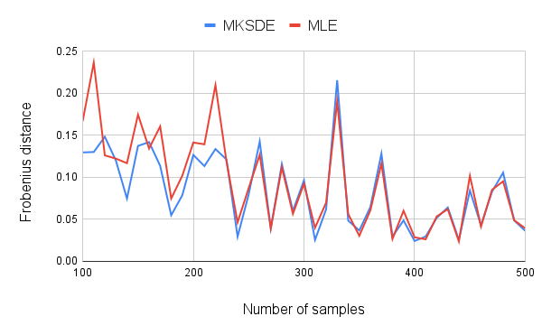
(a) $F_{0}=0.1*I$

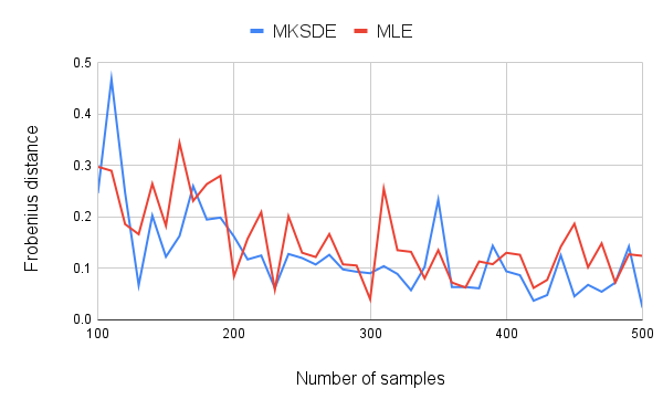
(b) $F_{0}=0.5*I$

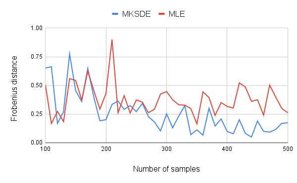
(c) $F_{0}=I$

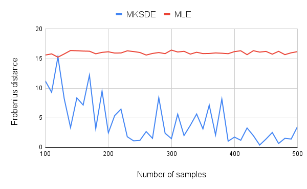
(d) $F_{0}=5*I$

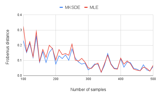
(e) $F_{0}=\text{diag}(0.1,0.2,0.3)$

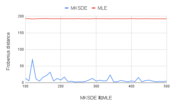
(f) $F_{0}=$ random

Figure 1: F-norms between estimators and ground truth

5.2 MKSDE goodness of fit test

The Cayley distribution [18] has the density $p(X|M)\propto\det(I+XM^{\top})^{\kappa}$ with parameters $M\in\operatorname{SO}(3)$ and $\kappa>0$. In this experiment, we measure the difference between a specific Cayley to the vMF family. As the vMF family is rotationally symmetric, the parameter $M$ does not affect the dissimilarity between a specific Cayley and the vMF family. We used the R package [37] to simulate $n=500$ samples from Cayley with different $\kappa$, and perform the goodness of fit test in §1 with different levels of significance $\beta$.

Table 1 presents the $(1-\beta)$-quantile and the statistic $nm^{*}_{n}$. As discussed in [18], the Cayley distribution resembles a uniform for small $\kappa$, and a spiky local Gaussian for large $\kappa$. It approximately belongs to the vMF in both cases, but differs from vMF for $\kappa$ in-between. This coincides with the results in table 1.

Table 1: MKSDE goodness of fit

$\kappa$	0.2	0.5	1.0	1.5	2.0
$n\cdot m^{*}_{n}$	68.65	90.25	99.99	99.29	104.23
$\beta=0.01$	83.98	94.23	108.18	116.88	139.76
$\beta=0.05$	77.62	83.21	96.99	104.18	114.47
$\beta=0.10$	73.22	77.79	90.71	96.46	107.12

6 Conclusions

In this paper, we presented a novel Stein’s operator defined on Lie Groups leading to a kernel Stein discrepancy (KSD) which is a normalization-free loss function. We presented several theoretical results characterizing the properties of this new KSD on Lie groups and the MKSDE. We presented new theorems on MKSDE being strongly consistent and asymptotically normal, and a closed form expression of the MKSDE for the vMF on $\operatorname{SO}(N)$. Finally, we presented experimental evidence depicting advantages of MKSDE over MLE.

In this paper, we did not delve in to the properties of local minimizers of KSD, while in many practical situations, a local minimizer is the best one can hope for. In our future work, we will develop the asymptotic theory of the local minimizers of KSD and/or possibly investigate efficient algorithms for realizing the theoretically established global minimizers in theorem 4.3.

Appendix A Derivations on $\operatorname{SO}(N)$

A.1 General Form of $k_{p}$ on $\operatorname{SO}(N)$

Theorem.

Given the kernel function $k(X,Y)=\exp(\tau\operatorname{tr}(X^{\top}Y))$, the function $k_{p}$ on $\operatorname{SO}(N)$ is given by,

$$k_{p}(X,Y) =\operatorname{tr}[\mathscr{A}(X^{\top}(\nabla_{X}\log p+\tau Y))^{\top}\mathscr{A}(Y^{\top}(\nabla_{Y}\log p+\tau X))]\cdot e^{\tau\operatorname{tr}(X^{\top}Y)}$$ (14)

$$+\frac{\tau}{2}(N-1)\operatorname{tr}(X^{\top}Y)e^{\tau\operatorname{tr}(X^{\top}Y)}.$$

Proof.

Let $\mathcal{A}^{ij}_{p}$ represent the the operator $\mathcal{A}^{l}_{p}$ corresponding to $E_{ij}$. Clearly,

$$\tilde{\mathcal{A}}^{ij}_{p}\mathcal{A}^{ij}_{p}k_{p}(X,Y) =\operatorname{tr}[(\nabla_{X}\log p+\tau Y)^{\top}XE_{ij}]\operatorname{tr}[(\nabla_{Y}\log p+\tau X)^{\top}YE_{ij}]\cdot e^{\tau\operatorname{tr}(X^{\top}Y)}$$ (15)

$$+\tau\operatorname{tr}(E^{\top}_{ij}X^{\top}YE_{ij})\cdot e^{\tau\operatorname{tr}(X^{\top}Y)}.$$

Recall that $E_{ij}$ is an orthonormal basis of the space Skew$(N)$ of all skew-symmetric matrices with the inner product $\langle\cdot,\cdot\rangle:=\operatorname{tr}(\cdot^{\top}\cdot)$. Note that $\operatorname{tr}(A^{\top}E_{ij})$ is the inner product of $A$ and $E_{ij}$, which actually equals $\operatorname{tr}(\mathscr{A}(A)^{\top}E_{ij})$, as $\mathscr{A}(A)$ is the orthogonal projection of $A$ onto the space Skew$(N)$. Furthermore, for any two matrices $A$ and $B$,

$$\sum_{i<j}\operatorname{tr}(A^{\top}E_{ij})\operatorname{tr}(B^{\top}E_{ij}) =\sum_{i<j}\operatorname{tr}(\mathscr{A}(A)^{\top}E_{ij})\operatorname{tr}(\mathscr{A}(B)^{\top}E_{ij})$$

$$=\sum_{i<j}\langle\mathscr{A}(A),E_{ij}\rangle\cdot\langle\mathscr{A}(B),E_{ij}\rangle$$

$$=\langle\mathscr{A}(A),\mathscr{A}(B)\rangle=\operatorname{tr}[\mathscr{A}(A)^{\top}\mathscr{A}(B)].$$

Therefore, the first term on the RHS in (15) becomes

$$\operatorname{tr}[\mathscr{A}(X^{\top}(\nabla_{X}\log p+\tau Y))^{\top}\mathscr{A}(Y^{\top}(\nabla_{Y}\log p+\tau X))]\cdot e^{\tau\operatorname{tr}(X^{\top}Y)}.$$

Moreover, note that $E_{ij}E^{\top}_{ij}$ equals the matrix which has all $0$s except two $(1/2)$s at $(i,i)^{th}$ and $(j,j)^{th}$ entry respectively. The sum of $E_{ij}E^{\top}_{ij}$, $1\leq i<j\leq N$ actually equals $\frac{N-1}{2}I$. Recall that one can commute matrices inside $\operatorname{tr}(\cdot)$, thus the second term on the RHS of (15) becomes,

$$c(X,Y):=\frac{\tau}{2}(N-1)\operatorname{tr}(X^{\top}Y)e^{\tau\operatorname{tr}(X^{\top}Y)}.$$

Combining the two terms we obtain the desired result. This completes the proof. ∎

A.2 Form of $k_{p}$ for vMF and RN on $\operatorname{SO}(N)$

vMF:

The gradient of $\log p=\operatorname{tr}(F^{\top}X)$ as a function in $\mathbb{R}^{N\times N}$ is exactly $F$, but we must project this gradient to the tangent space of $\operatorname{SO}(N)$ at $X$. The derivative of $\operatorname{tr}(F^{\top}X)$ w.r.t left-invariant field $E_{ij}$ at $X$ is $\operatorname{tr}(F^{\top}XE_{ij})$, which satisfies

$$\operatorname{tr}(F^{\top}XE_{ij})=\operatorname{tr}(\mathscr{A}(F^{\top}X)E_{ij})=\operatorname{tr}(\mathscr{A}(F^{\top}X)X^{\top}XE_{ij})=\langle X\mathscr{A}(X^{\top}F),XE_{ij}\rangle,\quad i<j.$$

Therefore, $X\mathscr{A}(X^{\top}F)$ is the gradient of $\operatorname{tr}(F^{\top}X)$. Substituting this in to (14) we have,

$$k^{\operatorname{vMF}}_{p}(X,Y)=c(X,Y)+\operatorname{tr}[\mathscr{A}(X^{\top}(F+\tau Y))^{\top}\mathscr{A}(Y^{\top}(F+\tau X))]\cdot e^{\tau\operatorname{tr}(X^{\top}Y)}.$$ (16)

RN:

The gradient of $\log p=-\frac{\varsigma}{2}\operatorname{tr}[\operatorname{Log}(\mu^{T}X)\operatorname{Log}(\mu^{\top}X)]$ at $X$ is $\nabla_{X}\log p=\varsigma\operatorname{Log}(X^{\top}\mu)$. Substituting this in to (14) leads to the following form:

$$k^{\text{RN}}_{p}=c+\operatorname{tr}[(\varsigma\operatorname{Log}(X^{\top}\mu)+\tau\mathscr{A}(X^{\top}Y))^{\top}(\varsigma\operatorname{Log}(Y^{\top}\mu)+\tau\mathscr{A}(Y^{\top}X))]\cdot e^{\tau\operatorname{tr}(X^{\top}Y)}.$$

A.3 Explicit form of MKSDE for vMF on $\operatorname{SO}(N)$

Theorem (MKSDE for vMF).

Given a group of samples $X_{i}\in\operatorname{SO}(N)$ modeled with vMF, the MKSDE is given by,

$$B=\frac{\tau}{2n^{2}}\sum_{i,j}(X_{i}-X_{j})\mathscr{A}(X_{i}^{\top}X_{j})e^{\tau\operatorname{tr}(X_{i}^{\top}X_{j})}\cdot\frac{q(X_{i})}{w(X_{i})}\cdot\frac{q(X_{j})}{w(X_{j})},\quad b=\operatorname{vec}{B},$$ (17)

$$A=\frac{1}{2n^{2}}\sum_{i,j}[I\otimes X_{i}X_{j}^{\top}-(X_{i}^{\top}\otimes X_{j})S_{N,N}]\cdot e^{\tau\operatorname{tr}(X_{i}^{\top}X_{j})}\cdot\frac{q(X_{i})}{w(X_{i})}\cdot\frac{q(X_{j})}{w(X_{j})}.$$

Proof.

It suffices to show the result for the unweighted case, since the weighted term $\frac{q(X_{i})}{w(X_{i})}\cdot\frac{q(X_{j})}{w(X_{j})}$ is independent of the parameter. For the properties of Kronecker product, we refer the readers to [40]. Specifically, one can easily check that $S_{N,N}\operatorname{vec}(F)=\operatorname{vec}(F^{\top})$.

Equation (16) can be rewritten as

$$k_{p}(X,Y) =c^{\prime}(X,Y)+\operatorname{tr}[\mathscr{A}(X^{\top}F)^{\top}\mathscr{A}(Y^{\top}F)]\cdot e^{\tau\operatorname{tr}(X^{\top}Y)}$$ (18)

$$-2\cdot\frac{\tau}{2}\operatorname{tr}[F^{\top}(X-Y)\mathscr{A}(X^{\top}Y)]\cdot e^{\tau\operatorname{tr}(X^{\top}Y)},$$

where $c^{\prime}$ is a term independent of $F$. Note that $k_{p}(X,Y)$ is a quadratic form in $F$. We convert the bi-linear forms into matrices. Note that

$$\operatorname{tr}[F^{\top}(X-Y)\mathscr{A}(X^{\top}Y)]=\operatorname{vec}[(X-Y)\mathscr{A}(X^{\top}Y)]^{\top}\cdot\operatorname{vec}(F),$$

thus we simply set $b(X,Y)=\frac{\tau}{2}\operatorname{vec}[(X-Y)\mathscr{A}(X^{\top}Y)]\cdot e^{\tau\operatorname{tr}(X^{\top}Y)}$.

For the second order form, first we split the equation as

$$\operatorname{tr}[\mathscr{A}(X^{\top}F)^{\top}\mathscr{A}(Y^{\top}F)]=\frac{1}{2}\operatorname{tr}[F^{\top}YX^{\top}F]-\frac{1}{2}\operatorname{tr}[F^{\top}YF^{\top}X]$$ (19)

For the first term

$$\operatorname{tr}[F^{\top}YX^{\top}F] =[(I\otimes X))\operatorname{vec}(F)]^{\top}\cdot[(I\otimes Y))\operatorname{vec}(F)]$$ (20)

$$=\operatorname{vec}(F)^{\top}\cdot(I\otimes X^{\top})\cdot(I\otimes Y)\cdot\operatorname{vec}(F)$$

$$=\operatorname{vec}(F)^{\top}\cdot(I\otimes X^{\top}Y)\cdot\operatorname{vec}(F).$$

For the second term,

$$\operatorname{tr}[F^{\top}YF^{\top}X] =\operatorname{vec}(F)^{\top}\cdot(X^{\top}\otimes Y)\cdot\operatorname{vec}(F^{\top})$$ (21)

$$=\operatorname{vec}(F)^{\top}\cdot(X^{\top}\otimes Y)S_{N,N}\cdot\operatorname{vec}(F)$$

Therefore, we set $A(X,Y)=\frac{1}{2}[I\otimes X^{\top}Y-(X^{\top}\otimes Y)\cdot S_{N,N}]\cdot e^{\tau\operatorname{tr}(X^{\top}Y)}$. Note that the MKSDE $\hat{F}$ is the minimizer of following quadratic form

$$\operatorname{vec}(F)^{\top}\cdot\sum_{i,j}A(X_{i},X_{j})\cdot\operatorname{vec}(F)-2\sum_{i,j}b(X_{i},X_{j})\cdot\operatorname{vec}(F),$$

which is what needs to be demonstrated. This completes the proof. ∎

Appendix B Proof of theorems

B.1 Proof of theorem 3.3

Theorem (Invariance of basis).

Suppose $A:=(a^{l}_{k})$ is the transformation between two basis $D^{l}$ and $E^{k}$ such that $D^{l}=\sum_{k}a^{l}_{k}E^{k}$, then the $\operatorname{KSD}$with basis $D^{l}$ and the $\overline{\operatorname{KSD}}$ with basis $E^{k}$ satisfies

$$\sqrt{\lambda_{\min}}\cdot\overline{\operatorname{KSD}}\leq\operatorname{KSD}\leq\sqrt{\lambda_{\max}}\cdot\overline{\operatorname{KSD}},$$ (22)

where, $\lambda_{\min}$ and $\lambda_{\max}$ are the smallest and largest eigenvalues of $A^{\top}A$.

Proof.

Let $\mathcal{T}_{p}$ be the Stein’s operator with basis $E^{k}$. Note that we have $\mathcal{A}^{l}_{p}h=\sum_{k}a^{l}_{k}\mathcal{T}^{k}_{p}h$ for $h\in\mathcal{H}_{k}$. This linear transformation also commutes with Bochner integral, that is, $\mathbb{E}_{q}[\vec{\mathcal{A}}_{p}f]=A\cdot\mathbb{E}_{q}[\vec{\mathcal{T}}_{p}f]$. Recall that $\operatorname{KSD}=\|\mathbb{E}_{q}[\vec{\mathcal{A}}_{p}f]\|_{\mathcal{H}^{d}_{k}}$ and $\overline{\operatorname{KSD}}=\|\mathbb{E}_{q}[\vec{\mathcal{T}}_{p}f]\|_{\mathcal{H}^{d}_{k}}$. The rest of the proof is standard. ∎

B.2 Proof of theorem 3.4

Theorem (Characterization).

Suppose $k$ is $C_{0}$-universal and $\sqrt{k_{p}(x,x)}$ is integrable with respect to locally Lipschitz densities $p$ and $q$. Suppose further $D^{l}\log(p/q)$ is $p$ and $q$-integrable for all $l$. Then $p=q\iff\operatorname{KSD}(p,q)=0$.

Proof.

We begin with the forward implication, "$\Rightarrow$". By [38, Cor. 4.36], we have $|\mathcal{A}_{p}f(x)|\leq\|f\|_{\mathcal{H}_{k}}\cdot\sqrt{k_{p}(x,x)}$ for $f\in\mathcal{H}_{k}$. Moreover, the RKHS of a $C_{0}$-universal kernel contains only $C_{0}$, thus bounded functions, see [3, Prop. 2.3.2]. Therefore, for all $f\in\mathcal{H}_{k}$, $f,\mathcal{A}_{p}f$ are both $q$-integrable. Next, recall that $\operatorname{div}(D^{l})=D^{l}\Delta$, thus $\operatorname{div}(pf_{l}D^{l})=p\cdot f_{l}D^{l}\Delta+p\cdot D^{l}f_{l}+f_{l}\cdot D^{l}p=\mathcal{A}^{l}_{p}f_{l}\cdot p$. By generalized Stokes’s theorem [7], if an integrable vector field on a complete manifold has integrable divergence, then its divergence integrates to $0$. Therefore, $\mathbb{E}_{p}[\mathcal{A}_{p}f]=\int_{G}\mathcal{A}_{p}f\cdot pd\mu=\int_{G}\operatorname{div}(\sum_{l=1}^{d}pf_{l}D^{l})d\mu=0$. For readers unfamiliar with the divergence operator or Stokes’s theorem, this proof maybe be interpreted as a general version of integration by parts on manifolds.

Now, we address the reverse implication, "$\Leftarrow$". Note that $\mathbb{E}_{q}[\mathcal{A}_{p}f]=\mathbb{E}_{q}[\mathcal{A}_{p}f-\mathcal{A}_{q}f]=\sum_{l}\mathbb{E}_{q}[f_{l}D^{l}\log(p/q)]$, since the operator $\mathcal{A}_{q}$ corresponding to $q$ also has the Stein’s identity. If $k$ is $C_{0}$-universal, then $\mathcal{H}_{k}$ is dense in the space of continuous functions vanishing at infinity [3, Thm. 4.1.1]. Since $\mathbb{E}_{q}[f^{l}D^{l}\log(p/q)]=0$ for all $f\in\mathcal{H}^{d}_{k}$, we have $D^{l}\log(p/q)=0$ for all $l$. As we assume $G$ is connected, $\log(p/q)$ is constant and thus $p=q$. ∎

B.3 Proof of theorem 4.1

Theorem (Asymptotic Distribution of KSD).

Suppose $V_{\alpha}(x,x)$ is $w$-integrable. For fixed $\alpha$,

1. $\operatorname{wKSD}_{n}(\alpha)\to\operatorname{KSD}(\alpha)$ almost surely;

2. If $p_{\alpha}\neq q$, $\sqrt{n}[\operatorname{wKSD}^{2}_{n}(\alpha)-\operatorname{KSD}^{2}(\alpha)]\xrightarrow{d.}N\big{(}0,4\text{var}_{y\sim w}[\mathbb{E}_{x\sim w}V_{\alpha}(x,y)]\big{)}$ .

3. If $p_{\alpha}=q$, then $n\operatorname{wKSD}^{2}_{n}(p_{\alpha},q)\xrightarrow{d.}\sum_{j=1}^{\infty}\lambda_{j}Z^{2}_{j}$, where $Z_{j}\overset{i.i.d}{\sim}N(0,1)$, $\lambda_{j}$ are the eigenvalues of the operator $g\mapsto\mathbb{E}_{y\sim w}[V_{\alpha}(\cdot,y)g(y)]$ s.t. $\sum_{j=1}^{\infty}\lambda_{j}=\mathbb{E}_{w}[V_{\alpha}(x,x)]$.

Moreover, $0\leq\inf_{\alpha}\operatorname{wKSD}^{2}_{n}(p_{\alpha},q)\leq\inf_{\alpha}\operatorname{KSD}^{2}(p_{\alpha},q)+O_{p}(n^{-1})$. In particular, if $q$ is contained in the family $p_{\alpha}$, then $\inf_{\alpha}\operatorname{wKSD}^{2}_{n}(p_{\alpha},q)\to\inf_{\alpha}\operatorname{KSD}^{2}(p_{\alpha},q)$ almost surely;

Proof.

Note that $V_{\alpha}(\cdot,\cdot)$ is also positive definite, thus $V_{\alpha}(x,y)^{2}\leq V_{\alpha}(x,x)V_{\alpha}(y,y)$, thus $\mathbb{E}_{q}[V_{\alpha}(x,x)]<+\infty$ implies that $\mathbb{E}_{x,y\sim q}[V_{\alpha}(x,y)^{2}]<+\infty$. Therefore, (1), (2) and (3) are straightforward from the classical asymptotic results of $V$-statistics [35, §6.4.1]. To show the last statement, note that for fixed $\alpha$, $\operatorname{wKSD}^{2}_{n}(\alpha)=\frac{n-1}{n}U_{n}+n^{-2}\sum_{i=1}^{n}V_{\alpha}(x_{i},x_{i})$, then $\operatorname{wKSD}^{2}_{n}(\alpha)\to\operatorname{KSD}^{2}(\alpha)$ almost surely by SLLN and the strong consistency of $U$-statistic [35, Thm. 5.4.A], with convergence rate of $O_{p}(n^{-1})$ by the convergence rate of $U$-statistic [35, Thm 5.4.B]. Take a sequence of $\alpha_{n}$ such that $\operatorname{KSD}(\alpha_{n})\leq\inf_{\alpha}\operatorname{KSD}(\alpha)+n^{-1}$, then

$$\inf_{\alpha}\operatorname{wKSD}_{n}(\alpha_{n})\leq\operatorname{wKSD}_{n}(\alpha_{n})=\operatorname{KSD}(\alpha_{n})+O_{p}(n^{-1})\leq\inf_{\alpha}\operatorname{KSD}(\alpha)+O_{p}(n^{-1}).$$

∎

B.4 Proof of theorem 4.2

Theorem.

Suppose $V_{(\cdot)}(\cdot,\cdot)$ is jointly continuous and $\sup_{\theta\in K}V_{\theta}(x,x)$ is $w$-integrable for any compact $K\subset\Theta$, then $\operatorname{wKSD}^{2}_{n}(\theta)\to\operatorname{KSD}^{2}(\theta)$ compactly almost surely, i.e., for any compact $K$,

$$\operatorname{wKSD}^{2}_{n}(\theta)\to\operatorname{KSD}^{2}(\theta)\text{ uniformly on }K,\quad\text{almost surely}.$$

As a corollary, if $\Theta$ is locally compact, $\operatorname{wKSD}_{n}$ and $\operatorname{KSD}$ are all continuous on $\Theta$.

Proof.

Note that $\operatorname{wKSD}_{n}(\theta):=\frac{n-1}{n}\frac{1}{n(n-1)}\sum_{i\neq j}V_{\theta}(x_{i},x_{j})+\frac{1}{n^{2}}\sum_{i=1}^{n}V_{\theta}(x_{i},x_{i})$. We apply a classical results [34, Thm. 1] regarding the uniform convergence of random functions. First, we show that $n^{-1}\sum_{i=1}^{n}V_{\theta}(x_{i},x_{i})\to\mathbb{E}_{q}[V_{\theta}(x,x)]$ compactly almost surely, thus $n^{-2}\sum_{i=1}^{n}V_{\theta}(x_{i},x_{i})$ tends to $0$ compactly almost surely. Second, we show that $\frac{1}{n(n-1)}\sum_{i\neq j}V_{\theta}(x_{i},x_{j})\to\operatorname{KSD}(\theta)$ compactly almost surely. These two statements together imply the theorem.

The first statement follows from a classical results [34, Thm. 1] regarding the uniform convergence of random functions. Then, it suffices to check the condition of equi-continuity. Take a sequence of compact sets $G_{n}$ such that $G=\bigcup G_{n}$, then the join continuity of $V_{(\cdot)}(\cdot,\cdot)$ will impies the joint uniform continuity of $V_{(\cdot)}(\cdot,\cdot)$ on $K\times G_{n}\times G_{n}$, which further implies the condition of equi-continuity.

The second statement follows from a results [43, Thm. 1] regarding the uniform convergence of $U$-statistic. Note that $V_{\theta}(\cdot,\cdot)$ is also a positive definite bivariate function, thus

$$\sup_{\theta\in K}|V_{\theta}(x,y)|\leq\sup_{\theta\in K}V_{\theta}(x,x)^{\nicefrac{{1}}{{2}}}\cdot\sup_{\theta\in K}V_{\theta}(y,y)^{\nicefrac{{1}}{{2}}},$$

Recall that the $w$-integrability of $\sup_{\theta\in K}V_{\theta}(x,x)$ implies the $w$-integrability of $\sup_{\theta\in K}V_{\theta}(x,x)^{\nicefrac{{1}}{{2}}}$ by Jensen’s inequality. Therefore, $\sup_{\theta\in K}|V_{\theta}(x,y)|$ is $w\times w$-integrable. The condition of the equi-continuity of $V_{(\cdot)}(x,y)$ is the same as the first statement. It suffices to show the equi-continuity of $\mathbb{E}_{y\sim w}[V_{(\cdot)}(\cdot,y)]$. For any compact $K\subset\Theta$, and any fixed $\theta_{0}\in K$, $x_{0}\in G$, we choose a compact neighborhood $W\subset G$ of $x_{0}$, and note that for any $\theta\in K$, $x\in W$ and any $y\in G$

$$V_{\theta}(x,y)\leq\sup_{\theta\in K,x\in W}[V_{\theta}(x,x)]^{\nicefrac{{1}}{{2}}}\cdot\sup_{\theta\in K}[V_{\theta}(y,y)]^{\nicefrac{{1}}{{2}}}.$$

Note that the right hand side is independent of $\theta\in K$ and $x\in W$, and is integrable in $y$ as the condition states. Therefore, regardless of any small perturbation on $\theta$ and $x$, the function $V_{\theta}(x,\cdot)$ will be uniformly bounded by some integrable function of $y$ that is independent of $\theta$ and $x$. Applying dominating convergence theorem, we conclude that $\mathbb{E}_{y\sim w}[V_{(\cdot)}(\cdot,y)]$ restricted on $K\times G$ is jointly continuous at $(\theta_{0},x_{0})$, and thus continuous on $K\times G$ by the arbitrariness of $\theta_{0}$ and $x_{0}$. It is thus uniformly continuous on $K\times G_{n}$ and hence the condition of equi-continuity holds.

The continuity of $\operatorname{wKSD}_{n}$ is straightforward since it is a finite summation of continuous functions. Since $\operatorname{KSD}$ is the uniform limit of $\operatorname{wKSD}_{n}$ on any compact set, $\operatorname{KSD}$ is continuous on any compact set. Therefore, $\operatorname{KSD}$ is continuous as continuity is a local property. This completes the proof. ∎

B.5 Proof of theorem 4.3

Theorem (Strong consistency).

Suppose the conditions in theorem 4.2 hold and $\Theta=\Theta_{1}\times\Theta_{2}$ such that $\Theta_{1}$ is compact, $\Theta_{2}$ is convex, and for each fixed $\theta_{1}\in\Theta_{1}$, $\operatorname{wKSD}_{n}(\theta_{1},\cdot)$ is convex on $\Theta_{2}$ and $\operatorname{KSD}(\theta_{1},\cdot)$ attains minimum value on a non-empty and compact set $\tilde{\Theta}_{0}(\theta_{1})\subset\text{int}(\Theta_{2})$. Then $\Theta_{0}$, $\widehat{\Theta}_{n}$ are non-empty for large $n$ and $\sup_{\theta\in\widehat{\Theta}_{n}}d(\theta,\Theta_{0})\to 0$ almost surely.

We establish some lemmas that will be needed for the proof.

Lemma B.1.

Suppose $f$ is convex and $C$ is a bounded open set. If there exists $x_{0}\in C$ such that $f(x_{0})<\inf_{x\in\partial C}f(x)$, then $\inf_{x\notin C}f(x)=\inf_{x\in\partial C}f$ and the set of global minimizers of $f$ is non-empty and contained in $C$.

Proof.

For all $x^{\prime}\notin C$, there exists $0\leq\beta<1$ such that $\beta x_{0}+(1-\beta)x^{\prime}\in\partial C$, and thus

$$\beta f(x_{0})+(1-\beta)f(x^{\prime})\geq f(\beta x_{0}+(1-\beta)x^{\prime})>f(x_{0})\Longrightarrow f(x^{\prime})>f(x_{0}).$$

Furthermore,

$$f(x^{\prime})\geq\beta f(x_{0})+(1-\beta)f(x^{\prime})\geq f(\beta x_{0}+(1-\beta)x^{\prime})\geq\inf_{x\in\partial C}f(x).$$

This concludes the proof. ∎

Note that $\Theta$ is locally compact, thus $\operatorname{wKSD}_{n}$ and $\operatorname{KSD}$ are continuous on $\Theta$ by theorem 4.3. Furthermore, as the pointwise limit preserves the convexity, $\operatorname{KSD}(\theta_{1},\cdot)$ is also convex in $\theta_{2}$ for all $\theta_{1}\in\Theta_{1}$. Let $m^{*}(\theta_{1}):=\inf_{\theta_{2}\in\Theta_{2}}\operatorname{KSD}(\theta_{1},\theta_{2})$, and denote by $\tilde{\Theta}_{0}(\theta_{1})$ the set of minimizers of $\operatorname{KSD}(\theta_{1},\cdot)$. Then we establish the next lemma.

Lemma B.2.

For each $\bar{\theta}_{1}\in\Theta_{1}$, there exists a neighborhood $V_{1}$ of $\bar{\theta}_{1}$ and a bounded open set $V_{2}\subset\Theta_{2}$ such that for any $\theta_{1}\in V_{1}$, $\tilde{\Theta}_{0}(\theta_{1})\subset V_{2}$.

Proof.

Take a bounded $V_{2}$ such that $\tilde{\Theta}_{0}(\bar{\theta_{1}})\subset V_{2}$, then since $\operatorname{KSD}(\bar{\theta}_{1},\cdot)-m^{*}(\bar{\theta}_{1})$ is continuous and positive on $\partial V_{2}$, let $\epsilon:=\inf_{\theta_{2}\in\partial V_{2}}\operatorname{KSD}(\bar{\theta}_{1},\theta_{2})-m^{*}(\bar{\theta}_{1})>0$. Note that $\{\bar{\theta}_{1}\}\times\partial V_{2}$ is a subset of the open set $\{\operatorname{KSD}(\cdot,\cdot)>\epsilon/2+m^{*}(\bar{\theta}_{1})\}$, thus we apply tube lemma [26, Lem. 26.8] and get an open neighborhood $V_{1}$ of $\bar{\theta}_{1}$ such that $V^{\prime}_{1}\times\partial V_{2}\subset\{\operatorname{KSD}(\cdot,\cdot)>\epsilon/2+m^{*}(\bar{\theta}_{1})\}$, which implies that $\inf_{V^{\prime}_{1}\times\partial V_{2}}\operatorname{KSD}>m^{*}(\bar{\theta}_{1})+\epsilon/2$. However, we choose a $\tilde{\theta}_{2}\in\tilde{\Theta}_{1}(\bar{\theta}_{1})\subset V_{2}$, there exists a neighborhood $V^{\prime\prime}_{1}$ of $\bar{\theta}_{1}$ such that $\sup_{\theta_{1}\in V^{\prime\prime}_{1}}\operatorname{KSD}(\theta_{1},\tilde{\theta}_{2})<m^{*}+\epsilon/2$, as $\operatorname{KSD}$ is continuous at $(\bar{\theta}_{1},\tilde{\theta}_{2})$. Therefore, for any $\theta_{1}\in V_{1}:=V^{\prime}_{1}\cap V^{\prime\prime}$, we have $\operatorname{KSD}(\theta_{1},\tilde{\theta}_{2})<\inf_{\theta_{2}\in\partial V_{2}}\operatorname{KSD}(\theta_{1},\theta)$. We now apply lemma B.1, resulting in the minimizer set $\tilde{\Theta}_{0}(\theta_{1})$ is contained in $V_{2}$. ∎

Now we are ready to prove the theorem.

Proof.

1. We show that $\Theta_{0}$ is non-empty.

Let $m^{*}_{0}:=\inf_{\theta_{1}\in\Theta_{1}}m^{*}(\theta_{1})=\inf_{\theta\in\Theta}\operatorname{KSD}(\theta)$. Take a sequence $\theta_{1,n}\in\Theta_{1}$ such that $m^{*}(\theta_{1,n})\downarrow m^{*}_{0}$. As $\Theta_{1}$ is compact, $\theta_{1,n}$ has a convergent sub-sequence, still denoted as $\theta_{1,n}$, whose limit point is denoted as $\theta_{1,0}$. We apply lemma B.2 to $\tilde{\Theta}_{0}(\theta_{1,0})$, thus there exists a compact neighborhood $V_{1}\times V_{2}$ of $\{\theta_{1,0}\}\times\tilde{\Theta}_{0}(\theta_{1,0})$ such that for all $\theta_{1}\in V_{1}$, $\tilde{\Theta}_{0}(\theta_{1})\subset V_{2}$. Since $\operatorname{KSD}$ is continuous on the compact set $\{\theta_{1,0}\}\times\tilde{\Theta}_{0}(\theta_{1,0})$ and the size of $V_{1}\times V_{2}$ can be taken as small as needed, we can shrink $V_{1}\times V_{2}$ such that $\inf_{\theta\in V_{1}\times V_{2}}\operatorname{KSD}(\theta)>m^{*}(\theta_{1,n})-\epsilon.$ However, note that $\theta_{1,n}$ will finally enter $V_{1}$, and from then on, $\{\theta_{1,n}\}\times\tilde{\Theta}_{0}(\theta_{1,n})\subset V_{2}$, which implies $\inf_{V_{1}\times V_{2}}\operatorname{KSD}(\theta)\leq m^{*}(\theta_{1,n})\downarrow m^{*}_{0}$. Therefore, $m^{*}(\theta_{1,n})-\epsilon<\inf_{V_{1}\times V_{2}}\operatorname{KSD}(\theta)\leq m^{*}(\theta_{1,n})\downarrow m^{*}_{0}$, and thus $m^{*}(\theta_{1,0})=m^{*}_{0}$ as $\epsilon$ is arbitrary. Therefore, $\Theta_{0}$ is non-empty.

2. We show that $\Theta_{0}$ is compact.

Suppose $\{B_{\alpha}\}\subset\Theta$ is a collection of open balls such that $\Theta_{0}\subset\bigcup B_{\alpha}$. For each $\theta_{1}$, the $\theta_{1}$-section $\Theta^{\theta_{1}}_{0}:=\{(\theta,\theta^{\prime})\in\Theta_{0}|\theta=\theta_{1}\}$ of $\Theta_{0}$, if non-empty, is exactly the set $\tilde{\Theta}_{0}(\theta_{1})$. Since $\Theta^{\theta_{1}}_{0}=\tilde{\Theta}_{0}(\theta_{1})$ is compact, there exists a finite subcollection of balls $B^{\theta_{1}}_{i}$, $1\leq i\leq n_{\theta_{1}}$ such that $\{\theta_{1}\}\times\tilde{\Theta}_{0}(\theta_{1})\subset\bigcup_{i}B^{\theta_{1}}_{i}$. We apply lemma B.2 to each $\theta_{1}$, and conclude there exists open neighborhoods $V^{\theta_{1}}_{1}$ and $V^{\theta_{1}}_{2}$ such that $\{\theta_{1}\}\times\tilde{\Theta}_{0}(\theta_{1})\subset V^{\theta_{1}}_{1}\times V^{\theta_{1}}_{2}\subset\bigcup_{i}B^{\theta_{1}}_{i}$. If the section $\Theta^{\theta_{1}}_{0}$ is empty, we prescribe $V^{\theta_{1}}_{1}$ and $V^{\theta_{2}}_{2}$ with arbitrary neighborhood such that $\{\theta_{1}\}\times\tilde{\Theta}_{0}(\theta_{1})\subset V^{\theta_{1}}_{1}\times V^{\theta_{1}}_{2}$. Note that $\{V^{\theta_{1}}_{1}\}_{\theta_{1}\in\Theta_{1}}$ is a open cover of $\Theta_{1}$, thus there exists an open cover $V^{\theta_{1,i}}_{1}$ for $\theta_{1,i}$, $1\leq i\leq n$. Note that $B^{\theta_{1,i}}_{j}$, $1\leq i\leq n$, $1\leq j\leq n_{\theta_{1,i}}$ is a finite subcover of $\Theta_{0}$. Therefore, $\Theta_{0}$ is compact.

3. We show that the minimizers $\widehat{\theta}_{n}\in\widehat{\Theta}_{n}$ will eventually enter a compact set uniformly.

Since $\Theta_{0}$ is compact, we choose an open set $K\subset\Theta_{2}$ with compact closure such that $\Theta_{0}\subset\Theta_{1}\times K$. Since $\operatorname{KSD}-m^{*}_{0}$ is continuous and positive on the compact set $\Theta_{1}\times\partial K$, let $\epsilon:=\inf_{\Theta_{1}\times\partial K}\operatorname{KSD}(\theta)-m^{*}_{0}>0$. By theorem 4.2, $\operatorname{wKSD}^{2}_{n}\to\operatorname{KSD}$ uniformly on $\Theta_{1}\times\bar{K}$, which implies for large enough $n$, $\operatorname{wKSD}_{n}>m^{*}_{0}+\epsilon/2$ uniformly on $\Theta_{1}\times\partial K$ and $\operatorname{wKSD}_{n}<m^{*}_{0}+\epsilon/2$ uniformly on $\Theta_{0}$. Therefore, we can apply lemma B.1 to each $\operatorname{wKSD}_{n}(\theta_{1},\cdot)$, and conclude that $\widehat{\Theta}_{n}\subset\Theta_{1}\times K$ for large enough $n$.

4. We show the theorem.

Since the global minimizers of $\operatorname{wKSD}_{n}$ will eventually enter the compact set $\Theta_{1}\times\bar{K}$. We assume that $\widehat{\Theta}_{n}$ is set of minimizers of $\operatorname{wKSD}_{n}$ over $\Theta_{1}\times\bar{K}$ WLOG.

For each $\delta>0$, let $\Theta_{\delta}:=\{\theta\in\Theta_{1}\times\bar{K}:d(\theta,\Theta_{0})<\delta\}$ be the closed $\delta$-neighborhood of $\Theta_{0}$ in $\Theta_{1}\times\bar{K}$, and let $\Theta^{c}_{\delta}:=\Theta_{1}\times\bar{K}-\Theta_{\delta}$. Note that $\Theta^{c}_{\delta}$ is compact, and $\operatorname{KSD}-m^{*}0$ is positive on $\Theta^{c}_{\delta}$, thus we let $\epsilon_{\delta}:=\inf_{\Theta^{c}_{\delta}}\operatorname{KSD}(\theta)-m^{*}_{0}>0$. For $n$ large enough such that $\widehat{\Theta}_{n}\subset\Theta_{1}\times\bar{K}$ and $\sup|\operatorname{wKSD}_{n}-\operatorname{KSD}|<\epsilon_{\delta}/2$, thus for each $\hat{\theta}_{n}\in\widehat{\Theta}_{n}$,

$$\operatorname{KSD}(\hat{\theta}_{n})-m^{*}_{0}<\operatorname{wKSD}_{n}(\hat{\theta}_{n})+\epsilon/2_{\delta}-m^{*}_{0}\leq\operatorname{wKSD}_{n}(\theta_{0})+\epsilon_{\delta}/2-m^{*}_{0}<m^{*}_{0}+\epsilon_{\delta}-m^{*}_{0}=\epsilon_{\delta},$$

which implies $\hat{\theta}_{n}\in\Theta_{\delta}$, thus proving the theorem. ∎

B.6 Proof of theorem 4.4

Theorem (CLT for MKSDE).

Let $\hat{\theta}_{n}$ be a sequence of MKSDE that converges to $\theta_{0}\in\Theta_{0}$. Suppose $\operatorname{KSD}^{2}(\theta)$ is at least $C^{2}$ in a neighborhood of $\theta_{0}$ and the Hessian $\mathcal{I}(\theta_{0})$ of $\operatorname{KSD}^{2}$ at $\theta_{0}$ is invertible. Then $\sqrt{n}[\mathcal{I}(\theta_{0})]^{\nicefrac{{1}}{{2}}}\operatorname{Log}_{\theta_{0}}(\hat{\theta}_{n})\xrightarrow{d.}\mathcal{N}(0,I)$. In more practical situations, we have $\sqrt{n}[\mathcal{I}(\hat{\theta}_{n})]^{\nicefrac{{1}}{{2}}}\operatorname{Log}_{\hat{\theta}_{n}}(\theta_{0})\xrightarrow{d.}\mathcal{N}(0,I)$.

Proof.

Throughout history, the asymptotic normality of the minimizer of a loss function is always established via a similar strategy to the classical results regarding the asymptotic normality of MLE, e.g, the asymptotic normality of MKSDE established in [2, 27].

In this work, since the parameter space may not be a vector space, we can not directly adopt their proof. However, as the MKSDE $\hat{\theta}_{n}$ converges to the ground truth $\theta_{0}$, the sequence will finally enter a neighborhood of $\theta_{0}$. Since a manifold is locally Euclidean, we may adopt their proof in a local chart of the manifold. It is convenient to take the normal coordinates given by the exponential map Exp${}_{\theta_{0}}$ at $\theta_{0}$, as the Jacobian of the Exp${}_{\theta_{0}}$ is $I$ at $0$ and the geodesic connecting $\hat{\theta}_{n}$ with $\theta_{0}$ coincides with the line segments connecting $\operatorname{Log}_{\theta_{0}}(\theta)$ with $0$ on the tangent space at $\theta_{0}$.

The rest of the proof is the same as the one given in [2, 27]. ∎

References

- Barp et al. [2018] Alessandro Barp, Chris Oates, Emilio Porcu, Mark Girolami, et al. A riemann-stein kernel method. arXiv preprint arXiv:1810.04946, 2018.
- Barp et al. [2019] Alessandro Barp, Francois-Xavier Briol, Andrew Duncan, Mark Girolami, and Lester Mackey. Minimum stein discrepancy estimators. Advances in Neural Information Processing Systems, 32, 2019.
- Carmeli et al. [2010] Claudio Carmeli, Ernesto De Vito, Alessandro Toigo, and Veronica Umanitá. Vector valued reproducing kernel hilbert spaces and universality. Analysis and Applications, 8(01):19–61, 2010.
- Chwialkowski et al. [2016] Kacper Chwialkowski, Heiko Strathmann, and Arthur Gretton. A kernel test of goodness of fit. In International conference on machine learning, pages 2606–2615. PMLR, 2016.
- Deng et al. [2022] Haowen Deng, Mai Bui, Nassir Navab, Leonidas Guibas, Slobodan Ilic, and Tolga Birdal. Deep bingham networks: Dealing with uncertainty and ambiguity in pose estimation. International Journal of Computer Vision, 130(7):1627–1654, 2022.
- Downs [1972] Thomas D Downs. Orientation statistics. Biometrika, 59(3):665–676, 1972.
- Gaffney [1954] Matthew P Gaffney. A special stokes’s theorem for complete riemannian manifolds. Annals of Mathematics, pages 140–145, 1954.
- Gilitschenski et al. [2020] Igor Gilitschenski, Roshni Sahoo, Wilko Schwarting, Alexander Amini, Sertac Karaman, and Daniela Rus. Deep orientation uncertainty learning based on a bingham loss. In International conference on learning representations, 2020.
- Gorham and Mackey [2015] Jackson Gorham and Lester Mackey. Measuring sample quality with stein’s method. Advances in Neural Information Processing Systems, 28, 2015.
- Gorham and Mackey [2017] Jackson Gorham and Lester Mackey. Measuring sample quality with kernels. In International Conference on Machine Learning, pages 1292–1301. PMLR, 2017.
- Gretton et al. [2009] Arthur Gretton, Kenji Fukumizu, Zaid Harchaoui, and Bharath K Sriperumbudur. A fast, consistent kernel two-sample test. Advances in neural information processing systems, 22, 2009.
- Helgason [1979] Sigurdur Helgason. Differential geometry, Lie groups, and symmetric spaces. Academic press, 1979.
- Hoff [2009] Peter D Hoff. Simulation of the matrix bingham–von mises–fisher distribution, with applications to multivariate and relational data. Journal of Computational and Graphical Statistics, 18(2):438–456, 2009.
- Khatri and Mardia [1977] CG Khatri and Kanti V Mardia. The von mises–fisher matrix distribution in orientation statistics. Journal of the Royal Statistical Society: Series B (Methodological), 39(1):95–106, 1977.
- Lee [2006] John M Lee. Riemannian Manifolds: An Introduction to Curvature. Springer Science & Business Media, 2006.
- Lee [2013] John M Lee. Introduction to Smooth Manifolds. Springer, 2013.
- Lee [2018] Taeyoung Lee. Bayesian attitude estimation with the matrix fisher distribution on so (3). IEEE Transactions on Automatic Control, 63(10):3377–3392, 2018.
- León et al. [2006] Carlos A León, Jean-Claude Massé, and Louis-Paul Rivest. A statistical model for random rotations. Journal of Multivariate Analysis, 97(2):412–430, 2006.
- Ley and Verdebout [2018] Christophe Ley and Thomas Verdebout. Applied directional statistics: modern methods and case studies. CRC Press, 2018.
- Ley et al. [2017] Christophe Ley, Gesine Reinert, and Yvik Swan. Stein’s method for comparison of univariate distributions. 2017.
- Liu et al. [2016] Qiang Liu, Jason Lee, and Michael Jordan. A kernelized stein discrepancy for goodness-of-fit tests. In International conference on machine learning, pages 276–284. PMLR, 2016.
- Mardia et al. [2000] Kanti V Mardia, Peter E Jupp, and KV Mardia. Directional statistics, volume 2. Wiley Online Library, 2000.
- Matsubara et al. [2022] Takuo Matsubara, Jeremias Knoblauch, François-Xavier Briol, and Chris J Oates. Robust generalised bayesian inference for intractable likelihoods. Journal of the Royal Statistical Society Series B: Statistical Methodology, 84(3):997–1022, 2022.
- Mijoule et al. [2018] Guillaume Mijoule, Gesine Reinert, and Yvik Swan. Stein operators, kernels and discrepancies for multivariate continuous distributions. arXiv preprint arXiv:1806.03478, 2018.
- Mijoule et al. [2021] Guillaume Mijoule, Gesine Reinert, and Yvik Swan. Stein’s density method for multivariate continuous distributions. arXiv preprint arXiv:2101.05079, 2021.
- Munkres [2000] James R Munkres. Topology. (No Title), 2000.
- Oates et al. [2022] Chris Oates et al. Minimum kernel discrepancy estimators. arXiv preprint arXiv:2210.16357, 2022.
- Oates et al. [2017] Chris J Oates, Mark Girolami, and Nicolas Chopin. Control functionals for monte carlo integration. Journal of the Royal Statistical Society. Series B (Statistical Methodology), pages 695–718, 2017.
- Oualkacha and Rivest [2012] Karim Oualkacha and Louis-Paul Rivest. On the estimation of an average rigid body motion. Biometrika, 99(3):585–598, 2012.
- Pennec [2006] Xavier Pennec. Intrinsic statistics on riemannian manifolds: Basic tools for geometric measurements. Journal of Mathematical Imaging and Vision, 25:127–154, 2006.
- Peretroukhin et al. [2020] Valentin Peretroukhin, Matthew Giamou, David M Rosen, W Nicholas Greene, Nicholas Roy, and Jonathan Kelly. A smooth representation of belief over so (3) for deep rotation learning with uncertainty. arXiv preprint arXiv:2006.01031, 2020.
- Petersen [2016] Peter Petersen. Riemannian Geometry. Springer, 2016.
- Prokudin et al. [2018] Sergey Prokudin, Peter Gehler, and Sebastian Nowozin. Deep directional statistics: Pose estimation with uncertainty quantification. In Proceedings of the European conference on computer vision (ECCV), pages 534–551, 2018.
- Rubin [1956] Herman Rubin. Uniform convergence of random functions with applications to statistics. The Annals of Mathematical Statistics, pages 200–203, 1956.
- Serfling [2009] Robert J Serfling. Approximation theorems of mathematical statistics. John Wiley & Sons, 2009.
- Sorenson [1985] H. W. Sorenson, editor. Kalman Filtering: Theory and Application. IEEE Press, 1985.
- Stanfill et al. [2014] Bryan Stanfill, Heike Hofmann, and Ulrike Genschel. rotations: An r package for so(3) data. The R Journal, 6:68–78, 2014. URL https://journal.r-project.org/archive/2014-1/stanfill-hofmann-genschel.pdf.
- Steinwart and Christmann [2008] Ingo Steinwart and Andreas Christmann. Support Vector Machines. Springer Science & Business Media, 2008.
- Suvorova et al. [2021] Sofia Suvorova, Stephen D Howard, and Bill Moran. Tracking rotations using maximum entropy distributions. IEEE Transactions on Aerospace and Electronic Systems, 57(5):2953–2968, 2021.
- Van Loan [2000] Charles F Van Loan. The ubiquitous kronecker product. Journal of computational and applied mathematics, 123(1-2):85–100, 2000.
- Wang and Lee [2021] Weixin Wang and Taeyoung Lee. Matrix fisher–gaussian distribution on and bayesian attitude estimation. IEEE Transactions on Automatic Control, 67(5):2175–2191, 2021.
- Xu and Matsuda [2021] Wenkai Xu and Takeru Matsuda. Interpretable stein goodness-of-fit tests on riemannian manifold. In International Conference on Machine Learning, pages 11502–11513. PMLR, 2021.
- Yeo and Johnson [2001] In-Kwon Yeo and Richard A Johnson. A uniform strong law of large numbers for u-statistics with application to transforming to near symmetry. Statistics & probability letters, 51(1):63–69, 2001.
- Zhang and Fletcher [2014] Miaomiao Zhang and P Thomas Fletcher. Bayesian principal geodesic analysis in diffeomorphic image registration. In Medical Image Computing and Computer-Assisted Intervention–MICCAI 2014: 17th International Conference, Boston, MA, USA, September 14-18, 2014, Proceedings, Part III 17, pages 121–128. Springer, 2014.
- Zhang and Fletcher [2013] Miaomiao Zhang and Tom Fletcher. Probabilistic principal geodesic analysis. Advances in neural information processing systems, 26, 2013.
- Zhang et al. [2019] Youshan Zhang, Jiarui Xing, and Miaomiao Zhang. Mixture probabilistic principal geodesic analysis. In Multimodal Brain Image Analysis and Mathematical Foundations of Computational Anatomy: 4th International Workshop, MBIA 2019, and 7th International Workshop, MFCA 2019, Held in Conjunction with MICCAI 2019, Shenzhen, China, October 17, 2019, Proceedings 4, pages 196–208. Springer, 2019.