Testing Multiband ($G$, $G_{\rm BP}$, $G_{\rm RP}$, $B$, $V$ and $TESS$) Standard Bolometric Corrections by Recovering Luminosity and Radii of 341 Host Stars

Abstract

Main-sequence bolometric corrections ($BC$) and a standard $BC-T_{\rm eff}$ relation are produced for TESS wavelengths using published physical parameters and light ratios from SED models of 209 detached double-lined eclipsing binaries. This and previous five-band (Johnson $B$, $V$, Gaia $G$, $G_{\rm BP}$, $G_{\rm RP}$) standard $BC-T_{\rm eff}$ relations are tested by recovering luminosity ($L$) of the most accurate 341 single host stars (281 MS, 40 subgiants, 19 giants and one PMS). Recovered $L$ of photometry are compared to $L$ from published $R$ and $T_{\rm eff}$. A very high correlation ($R^{2}$ = 0.9983) is achieved for this mixed sample. Error histograms of recovered and calculated $L$ show peaks at $\sim$2 and $\sim$4 per cent respectively. The recovered L and the published $T_{\rm eff}$ were then used in $L=4\pi R^{2}\sigma T^{4}_{\rm eff}$ to predict the standard $R$ of the host stars. Comparison between the predicted and published R of all luminosity classes are found successful with a negligible offset associated with the giants and subgiants. The peak of the predicted $R$ errors is found at 2 per cent, which is equivalent to the peak of the published $R$ errors. Thus, a main-sequence $BC-T_{\rm eff}$ relation could be used in predicting both $L$ and $R$ of a single star at any luminosity class, but this does not mean $BC-T_{\rm eff}$ relations of all luminosity classes are the same because luminosity information could be more constrained by star’s apparent magnitude $\xi$ than its $BC$ since $m_{\rm Bol}=\xi+BC_{\xi}$.

1 Introduction

Luminosity ($L$) is not an observable parameter for a star. There are only one direct and two indirect methods of obtaining $L$. The direct method uses the Stefan-Boltzmann law ($L=4\pi R^{2}\sigma T_{\rm eff}^{4}$) for calculating a luminosity directly from a given radius ($R$) and effective temperature ($T_{\rm eff}$) of a star. Therefore, the most accurate stellar $L$ comes from observationally determined most accurate $R$ and $T_{\rm eff}$ values which would be available from Detached Double-lined Eclipsing Binaries (DDEBs; Andersen, 1991; Torres et al., 2010; Eker et al., 2014; Eker et al., 2015, 2018). The typical accuracy of a calculated $L$ is 8.2–12.2 per cent (Eker et al., 2021b).

The first of the two indirect methods requires mass and pre-determined classical mass-luminosity relation (MLR) in the form of $L\propto M^{\alpha}$, where the typical accuracy is 17.5-37.99 per cent (Eker et al., 2018; Eker et al., 2021b). In early times, especially after the discovery of main-sequence MLR independently by Hertzsprung (1923) and Russell et al. (1923), the MLR was claimed to be one of the most prominent empirical laws of nature by Eddington (1926) and Gabovits (1938) and it was used either predicting $L$ from $M$ or $M$ from $L$ at least until the middle of the 20th century or perhaps until Andersen (1991) was objecting it. Those were the times the observational accuracy of $L$ (or $M$) was not high enough to distinguish the true $L$ (or $M$) from the average $L$ (or $M$) for a given $M$ (or $L$) of a main-sequence star.

The second of the two indirect methods requires an absolute visual magnitude and a pre-estimated bolometric correction ($BC$) to compute the absolute bolometric magnitude of a star in the first step as $M_{\rm Bol}$ = $M_{\rm V}$ + $BC_{\rm V}$ and then to obtain its $L$ in SI units from

$$M_{\rm Bol}=-2.5\times logL+71.197425...,$$ (1)

where the typical accuracy of $L$ is about to 10-13 per cent (Eker et al., 2021b, 2022; Bakış & Eker, 2022) which is equivalent to the uncertainty of $BC_{\rm V}$ if the uncertainty of the absolute visual magnitude is negligible and the $BC_{\rm V}$ is a standard $BC_{\rm V}$. Otherwise, that is if the $BC_{\rm V}$ is not a standard $BC_{\rm V}$, an additional uncertainty 10 per cent or more (Eker et al., 2021b, 2022) would arise due to the complexities caused by the three paradigms (the $BC$ scale is arbitrary, $BC$ values must always be negative, and the bolometric magnitude of a star ought to be brighter than its $V$ magnitude) which are not valid since 2015 (Eker et al., 2022). It was Torres (2010) who first noticed inconsistencies due to improper usage of $M_{Bol,\odot}$ and tabulated $BC_{\rm V}$ values that may lead to errors of up to 10 per cent or more in the derived $L$ equivalent to about 0.1 mag or more in the bolometric magnitudes.

Disagreed bolometric corrections ($BC_{\rm V}$), which are primarily in tabulated form, had been used for about a century (Kuiper, 1938; Popper, 1959; Johnson, 1966; Flower, 1996; Bessell et al., 1998; Girardi et al., 2008; Sung et al., 2013). International Astronomical Union was aware of the problem, thus, issued a general assembly resolution hereafter IAU 2015 GAR B2, to solve the problems associated with the arbitrariness attributed to the zero point constants of the $M_{\rm Bol}$ and $BC$ scales. This revolutionary document (Eker et al., 2022) appears to be ignored or its full potential was not understood properly since some authors continued the old tradition (Casagrande & VandenBerg, 2018; Andrae et al., 2018; Chen et al., 2019; Eker et al., 2020) under the influence of the paradigms. The revolution has been noticed first by Eker et al. (2021a) who revised the definition of standard bolometric correction according classical definition $BC_{\rm V}=M_{\rm Bol}-M_{\rm V}$ where $M_{\rm V}$ is calculated from an apparent magnitude, parallax, and interstellar extinction while $M_{\rm Bol}$ is calculated according to IAU 2015 GAR B2 (Eq.1) or using

$$M_{\rm Bol}=M_{bol,\odot}-2.5\times logL/L_{\odot}$$ (2)

in which the nominal solar values $M_{Bol,\odot}=$ 4.74 mag and $L_{\odot}=$ 3.828$\times 10^{26}$ W should be used during pre-computation of a $BC$ because the zero point constant of the bolometric magnitude scale $C_{\rm Bol}=M_{Bol,\odot}+2.5logL_{\odot}=71.197425...$ has been fixed by the General Assembly of IAU in 2015 meeting.

A predicted $L$ according to the third method using an absolute magnitude and a standard $BC$ could be called standard $L$ while a computed $L$ according to the Stefan-Boltzmann law is standard by the definition. Investigating typical and limiting accuracies of the three methods of obtaining stellar $L$ in the era after Gaia, Eker et al. (2021b) claimed that it is possible to predict a standard $L$ within a few per cent if the pre-required $BC_{\rm V}$ is measured directly from a high signal to noise ratio spectrum according to the following definition of $BC_{\rm V}$

$$BC_{\rm V}=2.5log\frac{f_{\rm V}}{f_{\rm Bol}}+C_{2}=2.5log\frac{\int_{0}^{\infty}S_{\lambda}(V)f_{\lambda}d\lambda}{\int_{0}^{\infty}f_{\lambda}d\lambda}+C_{2},$$ (3)

where $S_{\lambda}(V)$ is the sensitivity function of the $V$ magnitude system, and $f_{\lambda}$ is the monochromatic flux from a star, and $C_{2}=C_{\rm Bol}-C_{\rm V}$, in which $C_{\rm V}$ is the zero point constant for the $V$ system of magnitudes. This claim, however, was found inapplicable and speculative by Bakış & Eker (2022), who suggested an alternative way of increasing the accuracy of standard $L$ by using multiband standard $BC$s.

Bakış & Eker (2022) first determined the main-sequence standard $BC$ values for the photometric bands Gaia $G$, $G_{\rm BP}$, $G_{\rm RP}$ and Johnson $B$, $V$ from the most accurate stellar parameters of 406 main-sequence stars which are the components of 209 DDEBs contained in the catalogue of Eker et al. (2018). Then, $BC$ - $T_{\rm eff}$ relations of main-sequence stars were established for the same five photometric ($G$, $G_{\rm BP}$, $G_{\rm RP}$ and Johnson $B$, $V$) passbands. After, five $M_{\rm Bol}$ values of each star are estimated by $M_{\rm Bol}(\xi)$ = $M_{\xi}$ + $BC_{\xi}$, the mean $M_{\rm Bol}$ and its standard error is computed to represent the star in the list. At last, the standard $L$ of each star is obtained according to Eq.1 from its mean $M_{\rm Bol}$, while the standard error of $M_{\rm Bol}$ is propagated to be the uncertainty of the predicted $L$. Comparing predicted $L$ (from photometry) to the calculated $L$ (from SB) indicated a high degree of correlation ($R^{2}$ > 0.999). The most important is that comparing histogram distributions of errors showed that uncertainties associated with the predicted $L$ (peak at $\approx$ 2.5 per cent) are $\sim$3 times smaller than the uncertainties of $L$ (peak at $\approx$ 8 per cent) by the Stefan-Boltzmann law. There was no method providing $L$ more accurately than the direct method. Now, multiband $BC$s provides such an accuracy first in the history of astrophysics.

This study, however, is motivated for further testing of the multiband (Gaia $G$, $G_{\rm BP}$, $G_{\rm RP}$ and Johnson $B$, $V$) main-sequence $BC$ and $BC$ - $T_{\rm eff}$ relations by adding one more passband (TESS) in the series and applying them to the planet-hosting stars with most accurate $T_{\rm eff}$ and $R$. Not only by comparing predicted $L$ to calculated $L$ of the host stars, but also by comparing predicted $R$ to the published $R$. Choosing host stars sample not only among the main-sequence but also subgiants and giants, this study is also important for testing the claim of Flower (1996) who declared $BC$ values are the same for all luminosity classes including main-sequence, subgiants and giants even for the pre-main-sequence stars.

2 Data

The Transiting Exoplanet Survey Satellite (TESS) (Ricker et al., 2014, 2015), which was put into orbit in 2018, has led to important contributions to stellar and planetary astrophysics with its extremely sensitive photometric data (among hundreds of studies; Stassun et al., 2017; Fulton et al., 2017; Montalto, 2022). In addition to its numerous exoplanet discovery, which is the main mission of the satellite, it has also made important contributions to stellar astrophysics (among hundreds of studies; Günther et al., 2020; Antoci et al., 2019; Bakış et al., 2022; Espinoza & Jordán, 2016, for different kind of stellar objects). In the case of eclipsing binaries, it has become possible to obtain relative radii and light contribution of components with a precision better than 0.1 per cent.

On the way of estimating accurate absolute bolometric magnitudes and luminosity of the component stars of binaries using TESS light curves, interstellar dimming ($A_{\rm TESS}$) and the bolometric corrections ($BC_{\rm TESS}$) are two very critical parameters in addition to a sensitive Gaia distance (Gaia Collaboration et al., 2016). Despite there is a reliable source of obtaining these two parameters now exist at Johnson $B$, $V$ and Gaia $G$, $G_{\rm BP}$, $G_{\rm RP}$ band passes (Bakış & Eker (2022)), there is no reliable common source satisfying numerous researchers who are interested in solving TESS light curves of eclipsing binaries and exoplanet transiting light curves of single stars. This study, therefore, is devoted first to producing an empirical $E(B-V)$ - $A_{\rm TESS}$ relation for estimating $A_{\rm TESS}$ from the $E(B-V)$ colour excess of the system and then to calibrate an empirical main-sequence $BC$ - $T_{\rm eff}$ relation for the TESS pass band for estimating $BC_{\rm TESS}$ from the $T_{\rm eff}$ of the system. Note that, $A_{\rm TESS}$ is also needed in calculating $M_{\rm TESS}$ before obtaining mean $M_{\rm Bol}$ and its uncertainty for a star from six independent estimations of $M_{\rm Bol}(\xi)$ = $M_{\xi}$ + $BC_{\xi}$ including the TESS band. The standard $L$ of a star if computed from such a mean $M_{\rm Bol}$ using Eq.1 has already been shown to produce more accurate stellar $L$ than the classical direct method (Bakış & Eker, 2022) by a sample of DDEB components. Comparing L of the host star sample of this study will be an independent second test of multiband $BC$ - $T_{\rm eff}$ relations. At last, estimating the radii of host stars directly from this luminosity would be a second application tested in this study.

2.1 Data for establishing $BC_{\rm TESS}$ - $T_{\rm eff}$ relation

The same data set of 209 DDEBs from Bakış & Eker (2022) are used in this study also for estimating component light ratios ($l$) and interstellar extinction ($A_{\rm TESS}$) first in the TESS magnitudes by the same method and software involving SED and SIMBAD data as described by Bakış & Eker (2022). After eliminating the stars out of the main-sequence limits, which are the theoretical ZAMS and TAMS lines from PARSEC evolutionary models by Bressan et al. (2012), the number of component stars left on the main-sequence is 406 (197 binaries, 9 primaries and 3 secondaries). Furthermore, not all of the 209 systems have TESS apparent magnitudes. Therefore, we have been able to use only 390 main-sequence stars to establish $E(B-V)$ - $A_{\rm TESS}$ relation shown in Fig.1. It can be used in estimating interstellar dimming in TESS magnitudes if $E(B-V)$ colour excess is known.

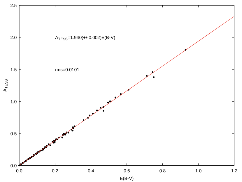
Figure 1: The $E(B-V)$ - $A_{\rm TESS}$ relation derived from 209 DDEB.

Table 1: Input parameters and $BC_{\rm TESS}$ values of DDEB stars with TESS apparent magnitudes. The full table is available online.

Order	Name	pri/sec	$R$	err	$T$	err	$L/L_{\odot}$	$L$(SI)	$\frac{\Delta L}{L}$	$M_{\rm Bol}$	err	$m({\rm sys})_{\rm TESS}$	err	$l_{\rm TESS}$	$m_{\rm TESS}$	Parallax	$\frac{\sigma_{\varpi}}{\varpi}$	$A_{\rm TESS}*$	$M_{\rm TESS}$	err	$BC_{\rm TESS}$	err
			[$R_{\odot}$]	[$\%$]	[$K$]	[$\%$]		$\times 10^{27}$	[%]	[mag]	[mag]	[mag]	[mag]		[mag]	[mas]	[%]	[mag]	[mag]	[mag]	[mag]	[mag]
1	V421 Peg	p	1.584	1.77	7250	1.10	6.245	2.390	5.66	2.751	0.061	7.936	0.006	0.614	8.465	6.5051	0.39	0.059	2.472	0.041	0.279	0.07
2	V421 Peg	s	1.328	2.18	6980	1.72	3.771	1.444	8.15	3.299	0.088	-	-	0.386	8.970	6.5051	0.39	0.059	2.977	0.041	0.322	0.10
3	DV Psc	p	0.685	4.38	4450	0.18	0.166	0.063	8.79	6.691	0.095	9.410	0.009	0.826	9.617	23.7216	0.09	0.370	6.123	0.041	0.569	0.10
4	DV Psc	s	0.514	3.89	3614	0.22	0.041	0.016	7.83	8.219	0.085	-	-	0.174	11.311	23.7216	0.09	0.370	7.817	0.041	0.402	0.09
5	MU Cas	p	4.192	1.19	14750	3.39	749.386	286.827	13.77	-2.447	0.149	10.549	0.020	0.555	11.187	0.5133	3.72	0.809	-1.070	0.092	-1.377	0.18
…	…	…	…	…	…	…	…	…	…	…	…	…	…	…	…	…	…	…	…	…	…	…
414	AP And	s	1.195	0.44	6495	2.31	2.291	0.877	9.28	3.840	0.101	-	-	0.476	11.313	2.9143	0.70	0.196	3.440	0.043	0.400	0.11
415	AL Scl	p	3.241	1.54	13550	2.58	319.014	122.103	10.78	-1.519	0.117	6.182	0.006	0.905	6.291	4.6006	3.63	0.021	-0.416	0.089	-1.104	0.15
416	AL Scl	s	1.401	1.43	10300	3.50	19.903	7.618	14.27	1.493	0.155	-	-	0.095	8.732	4.6006	3.63	0.021	2.026	0.089	-0.533	0.18
417	V821 Cas	p	2.308	1.21	9400	4.26	37.469	14.341	17.19	0.806	0.187	8.156	0.006	0.775	8.433	3.4262	0.59	0.061	1.047	0.042	-0.241	0.19
418	V821 Cas	s	1.390	1.58	8600	4.65	9.522	3.644	18.87	2.293	0.205	-	-	0.225	9.774	3.4262	0.59	0.061	2.388	0.042	-0.094	0.21
* Estimated uncertainty is 0.019 mag.

Once, the component light radios and the interstellar extinctions of 209 DDEB systems are known, and then it is straightforward to calculate $BC_{\rm TESS}$ of 390 main-sequence stars as shown by Table 1, where the columns are self-explanatory. Order, name of the system and the component (primary or secondary) are given in the first three columns. Only the parameters of 390 stars, a sample selected for this study with TESS magnitudes, are listed thus the numbers in the first column (order) are the same as given by Bakış & Eker (2022) for the readers who are interested in looking for the references of the published observed parameters, which are not given in this study to save space; that is, reducing the number of columns in the table. Columns 4, 5, 6 and 7 give radius ($R$), the relative error of $R$, effective temperature ($T_{\rm eff}$) and relative error of $T_{\rm eff}$, from which the luminosity ($L$) of each component is computed according to the Stefan Boltzmann law (column 8) in solar units. It is translated to SI units in column 9. The relative uncertainty of the computed $L$ in column 10 is the propagated uncertainty estimated from the random observational uncertainties of observed $R$ and $T_{\rm eff}$. Absolute bolometric magnitudes ($M_{\rm Bol}$) and corresponding uncertainties in columns 11 and 12 are calculated according to Eq.1 from the computed $L$. This completes the first step of obtaining $BC_{\rm TESS}$ of the component stars of the DDEB sample (Table 1) according to the classical definition $BC_{\rm TESS}$ = $M_{\rm Bol}$ - $M_{\rm TESS}$.

The second step, obtaining $M_{\rm TESS}$ requires apparent brightness of the system $[m({\rm sys})_{\rm TESS}]$, a light ratio of components ($l_{\rm TESS}$), a parallax ($\varpi$) and an interstellar extinction ($A_{\rm TESS}$). Column 13 and 14 retain brightness of the system $[m({\rm sys})_{\rm TESS}]$ and its associated uncertainty $[\Delta m({\rm sys})_{\rm TESS}]$ from the TESS catalogue (Stassun et al., 2018). The light ratio of components (column 15) is calculated as described by Bakış & Eker (2022) using the TESS bandpass curve (Sullivan et al., 2015) in the form of component contributions ($l_{pri}+l_{sec}=1$) that is the total contribution of primary and secondary is equal to one. Observational uncertainties $(\Delta m_{\rm TESS})$ of component’s magnitudes are assumed to be the same as systemic magnitudes $[\Delta m({\rm sys})_{\rm TESS}]$ (column 14) as done by Bakış & Eker (2022), therefore, $(m_{\rm TESS})$ in column 16 are given without uncertainty in the table. Columns 17 and 18 copy the parallaxes and associated relative errors directly from Bakış & Eker (2022) mostly from EDR3, which are checked and confirmed to be the same as Gaia DR3 parallaxes. Column 19 presents interstellar extinctions for the TESS photometry ($A_{\rm TESS}$) predicted in this study with an estimated accuracy of $0.019$ mag. Next, the absolute magnitude of a component ($M_{\rm TESS}$) and its propagated uncertainty are listed in columns 20 and 21. At last in the third step, the $BC_{\rm TESS}$ of a component (column 22) is found by subtracting $M_{\rm TESS}$ (column 20) from $M_{\rm Bol}$ (column 11). The last column (column 23) gives the propagated uncertainty computed from the uncertainties of the absolute bolometric and TESS magnitudes (column 23).

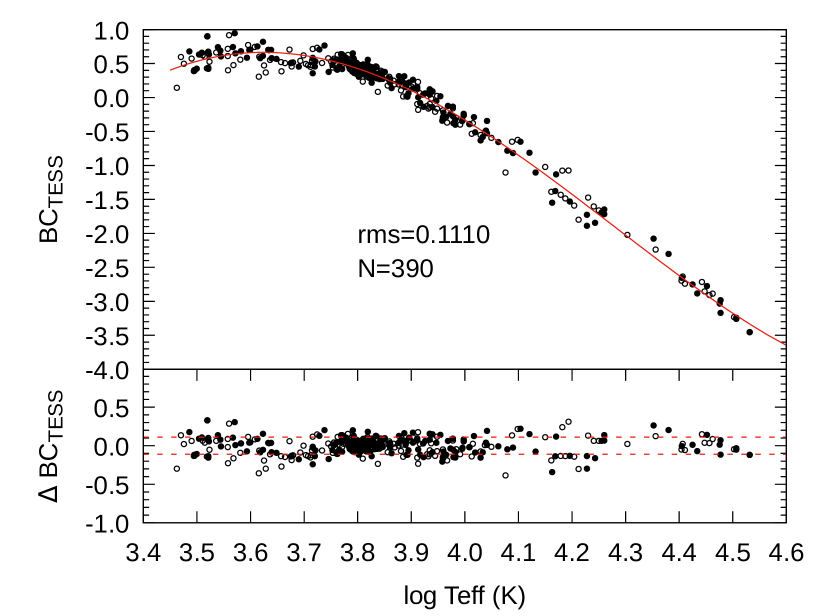
Figure 2: Distribution of empirical standard $BC_{\rm TESS}$ from 209 DDEB. Filled and empty circles are primaries and secondaries, respectively. The best fitting line represents empirical standard $BC_{\rm TESS}$ - $T_{\rm eff}$ relation. The number of stars ($N$) and RMS are indicated. One sigma deviation from the best-fitting curve is shown below.

2.2 Data for expanding $BC$ - $T_{\rm eff}$ relations

Empirical standard $BC_{\rm TESS}$ from the published $R$ and $T_{\rm eff}$ of 390 DDEB main-sequence components are displayed in Fig.2 where the continuous line is the best fitting curve. Coefficients and associated uncertainties are listed in Table 2 together with other $BC-T_{\rm eff}$ relations all in the forms of fourth-degree polynomials from Bakış & Eker (2022) representing the photometric bands of Johnson $B$, $V$, Gaia $G$, $G_{\rm BP}$ and $G_{\rm RP}$, where the uncertainties of the coefficients are shown by $\pm$ symbol. We have tried to fit both of the third and fourth-degree polynomials to the $BC_{\rm TESS}$ of this study, nevertheless, the fit of the third-degree polynomial is found better with a smaller RMS and more meaningful errors associated with the coefficients while the curves of both functions are very similar. Using the values of $a$, $b$, $c$, $d$ and $e$ from the table, one can calculate

$$BC_{\xi}=a+bX+cX^{2}+dX^{3}+eX^{4},$$ (4)

of any photometric band, where $X=log\,T_{\rm eff}$. The lower part of Table 2 is for comparing standard deviations (RMS), correlations ($R^{2}$) and the standard $BC$ of a main sequence star having a $T_{\rm eff}$ similar to the Sun ($T_{\rm eff}$ = 5772 K). The smallest RMS, which is 0.1092 mag, occurs at Gaia $B_{\rm RP}$ band, while the largest RMS, which is 0.1363 mag, occurs at Johnson $B$ band. The RMS of the TESS band has a moderate value (0.1110 mag) in between these limits. Note that the RMS values of each band determine the limiting accuracy of $M_{\rm Bol}$ sınce $M_{\rm Bol}$ = $M_{\xi}+BC_{\xi}$ under the condition the uncertainty of $M_{\xi}$ is negligible. The Maximum $BC$ values ($BC_{\rm max}$) occurring at effective temperature $T_{\rm max}$ are given below the absolute and apparent magnitudes if the main-sequence star with $T_{\rm eff}$ = 5772 K is shown by symbols $M_{\odot}$ and $m_{\odot}$ in the table. The lowest part of the table indicates the range of positive $BC$ values if exist. Accordingly, the $BC$ values of Johnson $B$ and Gaia $G_{\rm BP}$ bands are always negative. The $BC$ values of Johnson $V$ and Gaia $G$ bands would produce positive $BC$ values in the middle temperatures; for the $V$ band if 5300 < $T_{\rm eff}$ < 7830 K, for the G band if 4565 < $T_{\rm eff}$ < 4720 K. The $BC$ values of Gaia $G_{\rm RP}$ are positive if $T_{\rm eff}$ < 5890 K, while the $BC_{\rm TESS}$ are positive if $T_{\rm eff}$ < 8425 K. The relations are set valid for the main-sequence stars within the temperature range 2900-38000 K as it is implied by the sample of DDEB used in the calibrations.

Independently calibrated multiband standard $BC$ - $T_{\rm eff}$ relations are plotted all together in Fig.3. Except $TESS$ (thick solid) and $G_{\rm RP}$ (dashed) curves, which are similar, all of the other curves deviate from each other, especially towards lowest temperatures while all curves cross each other at $T_{\rm eff}$$\approx$10000 K and appear not deviating from each other $T_{\rm eff}>$10000 K as much as lower temperatures.

Figure 3: Independently calibrated six-band standard $BC$ - $T_{\rm eff}$ relations. The names of the passbands are indicated.

Each curve in Fig.3 could be used to estimate a $BC$ of a star at a photometric band preferred if its effective temperature were known. Because $BC$ - $T_{\rm eff}$ relations are independently calibrated and because observations at different photometric bands are independent, the predicted values of $M_{\rm Bol}$ of various bands would be independent. The six independent $M_{\rm Bol}$ for a single star could then be combined by taking an average. At last, the standard $L$ of a star is calculated from the averaged $M_{\rm Bol}$. Otherwise, each $M_{\rm Bol}$ providing a standard $L$ would be less accurate than the limiting accuracy indicated by the RMS values in Table 2.

Table 2: Coefficients of the fourth-degree polynomials ($BC$ - $T_{\rm eff}$ relations) for estimating $BC_{\xi}$, where $\xi$ could be one of the Johnson $B$, $V$, Gaia $G$, $G_{\rm BP}$, $G_{\rm RP}$ and TESS bands

Coefficient	$BC_{\rm B}^{*}$	$BC_{\rm V}^{*}$	$BC_{G}^{*}$	$BC_{G_{\rm BP}}^{*}$	$BC_{G_{\rm RP}}^{*}$	$BC_{\rm TESS}$
a	–1272.43	–3767.98	–1407.14	–3421.55	–1415.67	–318.533
	$\pm$394.2	$\pm$288.8	$\pm$256.7	$\pm$293.6	$\pm$253.3	$\pm$18.92
b	1075.85	3595.86	1305.08	3248.19	1342.38	232.298
	$\pm$394.4	$\pm$290.9	$\pm$258.9	$\pm$296.1	$\pm$255.4	$\pm$14.4
c	–337.831	–1286.59	–453.605	–1156.82	–475.827	–55.2916
	$\pm$147.7	$\pm$109.6	$\pm$97.67	$\pm$111.7	$\pm$96.34	$\pm$3.642
d	46.8074	204.764	70.2338	183.372	74.9702	4.27613
	$\pm$24.53	$\pm$18.32	$\pm$16.34	$\pm$18.68	$\pm$16.12	$\pm$0.3061
e	–2.42862	–12.2469	–4.1047	–10.9305	–4.44923	0
	$\pm$1.552	$\pm$1.146	$\pm$1.023	$\pm$1.169	$\pm$1.009	-
rms	0.136257	0.120071	0.11068	0.126577	0.109179	0.110951
$R^{2}$	0.9616	0.9789	0.9793	0.9738	0.9884	0.9847
$BC_{\odot}$ (mag)	–0.600	0.069	0.106	–0.134	0.567	0.517
$M_{\odot}$ (mag)	5.340	4.671	4.634	4.874	4.173	4.223
$m_{\odot}$ (mag)	–26.232	–26.901	–26.938	–26.698	–27.399	–27.349
$BC_{\rm max}$ (mag)	–0.301	0.094	0.106	–0.062	0.709	0.664
$T_{\rm max}$ (K)	8222	6397	5715	6879	4345	4210
$T_{1}$ (K)	-	5300	4565	-	-	-
$T_{2}$ (K)	-	7830	7420	-	8590	8425
*: Bakış & Eker (2022).

2.3 Data for Testing $BC$ - $T_{\rm eff}$ Relations

Five band ($B$, $V$, $G$, $G_{\rm RP}$ and $G_{\rm BP}$) $BC$ and $BC$ - $T_{\rm eff}$ relations has already been tested by Bakış & Eker (2022) by a sample of DDEB components from which $BC_{\xi}$ were computed and $BC_{\xi}$ - $T_{\rm eff}$ calibrated, where $\xi$ is any of the five photometric bands. Simply because DDEB are known to provide the most accurate stellar parameters (Andersen, 1991; Torres, 2010; Eker et al., 2014; Eker et al., 2015, 2018) and are already ready for such a test. The next most accurate stellar parameters appear to be coming from single stars which are hosting one or more exoplanets discovered by radial velocity variations and/or transiting light curves. High resolution and high signal-to-noise ratio spectra provide reliable $log\,g$ and $T_{\rm eff}$ of the host stars, while relatively shallow transits detected by ultra-high signal to ration light curves like TESS, on the other hand, resemble eclipses of DDEB, from which stellar $R$ and $M$ could be estimated at about $\sim 8$ per cent and 30 per cent (Stassun et al., 2017) using the direct observables. Later, the method is revised to provide host star $R$ and $M$ at a level of 10 per cent and 25 per cent by Stassun et al. (2018). At last, with the improved parallaxes of DR2 at the time and using granulation based $log\,g$ via Fourier background modelling (Corsaro et al., 2017) with TESS, the accuracy reached to 3 and 10 per cent levels respectively, which appear ideal for testing existing multiband $BC$ and $BC$ - $T_{\rm eff}$ relations by a different sample of stars other than DDEB components.

Host star physical parameters and associated errors are listed in NASA Exoplanet Archive together with the physical and orbital parameters of the confirmed planets. There was 5081 confirmed exoplanet belonging to 3799 host stars at the time when we downloaded the planetary systems composite data, from which we have selected 306 host stars having the most accurate $R$ and $T_{\rm eff}$ both within 2 per cent of accuracy for our preliminary list. This way, host stars with the most accurate stellar $L$ at all luminosity classes were collected intentionally in order to see how good existing main-sequence multiband $BC$ - $T_{\rm eff}$ relations are usable to other stages of evolution. Noting that the $L$ of a star primarily depends on its mass and metallicity, which is critical to identify sub-giants and main-sequence stars on H-R diagram, the host stars with a published metallicity were preferred. Because of the note “Data may not be self-consistent if drawn from multiple sources” on the table of Planetary Systems Composite Data, we have studied each star from its original sources to make sure self-consistency. In the second step, where we had to replace some of the original choices of $R$ and $T_{\rm eff}$ with a new $R$ and $T_{\rm eff}$ together with their associated uncertainty for the sake of consistency. We preferred not to discard a host star if the uncertainty of the new entry is bigger than 2 per cent but less than 3 per cent. Additional host stars fitting the selection criteria were also added thus our final list is enlarged to have 350 host stars.

However, during the process of estimating interstellar dimming of the selected host stars one by one from their un-reddened and reddened SED fitting, the following six systems KELT-21, WASP-118, HATS-37, Kepler-38, Kepler-1647 and Kepler-1661 were discarded because they have secondaries polluting their SED. The bright host $\alpha$ Tau was also discarded because it does not have Gaia apparent magnitudes. We had no choice but to discard the host K2-374 because its observed spectrophotometric fluxes could not be reached and the host K2-127 was discarded because its observed spectrophotometric fluxes were found not to fit its SED.

The sample containing 341 hosts selected for this study for testing multiband $BC$ and $BC$ - $T_{\rm eff}$ relations are listed in Table 3. Order and the star name are in columns 1 and 2 while parallax, error and reference are in columns 3, 4, and 5. Columns 6, 7 and 8 indicate radius, radius error and reference while columns 9, 10, 11 and 12 show spectral type, $T_{\rm eff}$, temperature error and reference. Column 13 is the luminosity class determined by us using ZAMS and TAMS lines of PARSEC models (Bressan et al., 2012) according to the published metallicity. The luminosity according to the Stefan-Boltzmann law from the observed $R$ and $T_{\rm eff}$ in solar and SI units are in columns 14 and 15 respectively while its propagated relative uncertainty ($\Delta L/L$) is in column 16. Corresponding $M_{\rm Bol}$ and uncertainty in the magnitude scale according to Eq.1 are given in columns 17 and 18.

Observational random errors of $R$ and $T_{\rm eff}$ are compared to the propagated errors of $L$ in Fig.4, where a much wider distribution of $L$ errors with a peak at 5 per cent caused by the powers of $R$ and $T_{\rm eff}$ is obvious. Fig.5 displays the positions of the sample host stars on the H-R diagram where the luminosity classes are indicated. Thus, the single host star sample contains 281 main-sequence (V), 40 sub-giants (IV), 19 giants and one pre-main-sequence (PMS) star YSES-2 (Bohn et al., 2021).

Table 3: The sample of host stars with most accurate radii and effective temperatures chosen for testing $BC$ and $BC-T_{\rm eff}$ relations.

Order	Host	Parallax	$\frac{\sigma_{\varpi}}{\varpi}$	Plx	$R$	err	Reference	Sp.	$T$	err	Reference	Lum.	$L/L_{\odot}$	$L$(SI)	$\frac{\Delta L}{L}$	$M_{\rm Bol}$	err
	Name	[mas]	[%]	Source	[$R_{\odot}$]	[$R_{\odot}$]		Type	[K]	[K]		Class		$\times 10^{27}$	[%]	[mag]	[mag]
1	16 Cyg B	47.3302	0.0362	DR3	1.13	0.01	2017AJ….153..136S	G3 V	5750	8	2017AJ….153..136S	V	1.258	0.481	1.9	4.491	0.020
2	24 Sex	13.6402	0.1960	DR3	4.90	0.08	2011AJ….141…16J	K0 IV	5098	44	2011AJ….141…16J	III	14.611	5.592	4.8	1.828	0.052
3	2MASSJ08421149+1916373	5.4387	0.3377	DR3	0.83	0.01	2016A&A…588A.118M	0	5300	30	2016A&A…588A.118M	V	0.486	0.186	3.7	5.523	0.040
4	55 Cnc	79.4482	0.0540	DR3	0.96	0.02	2021ApJS..255….8R	K0 IV-V	5318	81	2021ApJS..255….8R	V	0.664	0.254	7.4	5.185	0.080
5	61 Vir	117.1726	0.1243	DR3	0.96	0.01	2010ApJ…708.1366V	G5 V	5577	33	2010ApJ…708.1366V	V	0.808	0.309	3.3	4.971	0.036
…	…	…	…	…	…	…	…	…	…	…	…	…	…	…	…	…	…
337	WASP-187	2.7780	0.6339	DR3	2.83	0.05	2020MNRAS.499..428S	F	6150	89	2020MNRAS.499..428S	V	10.322	3.951	6.8	2.206	0.073
338	WASP-189	10.0997	0.2901	DR3	2.36	0.03	2020A&A…643A..94L	A	8000	80	2020A&A…643A..94L	V	20.553	7.867	4.7	1.458	0.051
339	XO-2 N	6.6588	0.2367	DR3	0.99	0.01	2012ApJ…761….7C	K0 V	5332	57	2015A&A…575A.111D	V	0.714	0.273	4.6	5.106	0.050
340	XO-7	4.3216	0.3066	DR3	1.48	0.02	2020AJ….159…44C	G0 V	6250	100	2020AJ….159…44C	V	3.011	1.153	7.1	3.543	0.077
341	YSES 2	9.1537	0.1291	DR3	1.19	0.02	2021A&A…648A..73B	K1 V	4749	40	2021A&A…648A..73B	PMS	0.652	0.250	5.0	5.204	0.054

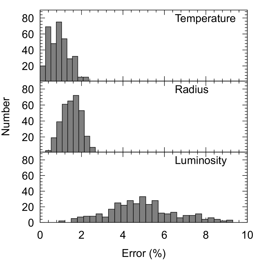
Figure 4: Error distributions of effective temperatures, radii and luminosity of 341 single host-stars in the present sample.

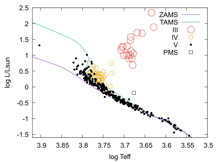
Figure 5: HR diagram of the host stars sample. The main sequence limits indicated by ZAMS and TAMS of the solar metallicity (Z=0.014) from PARSEC models (Bressan et al., 2012) while large empty circles are giants, medium empty circles are sub-giants, small filled circles are main-sequence stars and the empty square is a pre-main-sequence star.

3 Calculations

3.1 Estimating interstellar extinction using SED

Assuming a star is a black body having a temperature $T_{\rm eff}$ and if there is no interstellar extinction, a spherical star of size $R$ would produce a continuum flux (SED) at a distance $d$ from its centre. Putting this star at the $d$ parsec away from the Earth, according to the notation of Bakış & Eker (2022), its monochromatic flux above the atmosphere is

$$f_{\lambda}=\frac{R^{2}}{d^{2}}\pi B_{\lambda}(T_{\rm eff}).$$ (5)

where $\pi B_{\lambda}(T_{\rm eff})$ is monochromatic surface flux and $R^{2}$/$d^{2}$ is the dilution factor.

Using the parallaxes ($\varpi$), radii ($R$) and effective temperatures ($T_{\rm eff}$) in Table 3, the unreddened SED of the host stars in this study are computed in units of $Wm^{-2}$ Å^-1 and compared to their observed spectrophotometric flux data from the SIMBAD database (Wenger et al., 2000). For the nearby hosts with no interstellar extinction, like $\sigma$ Boo in the upper panel of Fig.6, the SED are found to fit perfectly to observed spectrophotometric flux data at all wavelengths. But, for the hosts with interstellar extinction like TOI-4329, the observed data towards the short wavelengths would be found off while the fit towards the long wavelengths appears acceptable to confirm the observed input parameters ($\varpi,R$ and $T_{\rm eff}$ ) are consistent. Inconsistency occurs if one or all of the observed parameters are determined wrongly and/or there is excess radiation in the system, which could be due to radiating circumstellar dust or flux from a companion star if the host is not a single star but a close binary.

The reddened SED of the host stars is modelled one by one by adjusting $E(B-V)$ of the system until a best-fitting reddened SED is obtained using the reddening model of Fitzpatrick (1999). Unreddened SED and best fitting reddened SED of the host star TOI-4329 are shown together in the lower panel of Fig.6.

Filter transition profiles, $S_{\lambda}(\xi)$, of the photometric bands Johnson $B$, $V$, Gaia $G$, $G_{\rm BP}$, $G_{\rm RP}$ and $TESS$ are needed to calculate interstellar extinctions, $A_{\xi}$,

$$A_{\xi}=2.5log\frac{\int_{0}^{\infty}S_{\lambda}(\xi)f_{\lambda}^{0}d\lambda}{\int_{0}^{\infty}S_{\lambda}(\xi)f_{\lambda}d\lambda},$$ (6)

where it is clear that if un-reddened $f_{\lambda}^{0}$ and reddened $f_{\lambda}$ are the same, $E(B-V)$ and all $A_{\xi}$ would be zero, which means no interstellar extinction. The filter profiles of the photometric bands are displayed in Fig.7 where transmission data for Johnson $B$ and $V$ are taken from Bessell (1990), Gaia passbands from Evans et al. (2018) and TESS from Sullivan et al. (2015). The passband-based interstellar extinctions determined by equation 6 for the host stars in this study are given in Table 4 together with apparent magnitudes.

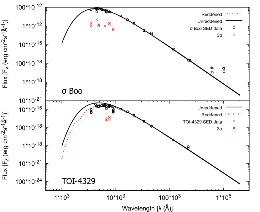
Figure 6: SED data and model for $\sigma$ Boo (top) and TOI 4329 (bottom). The data refers to within 5 arcsecs around the objects.

Figure 7: Transmission curves of photometric passband used in SED analysis.

Table 4: Apparent magnitudes and extinctions of the host stars sample at Johnson $B$, $V$, Gaia $G$, $G_{\rm BP}$, $G_{\rm RP}$ and TESS passbands. The full table is available online.

Order	Hostname	$B$	err	$V$	err	$G$	err	$G_{\rm BP}$	err	$G_{\rm RP}$	err	$TESS$	err	$A_{\rm B}*$	$A_{\rm V}*$	$A_{G}*$	$A_{GBP}*$	$A_{GRP}*$	$A_{\rm TESS}*$
		[mag]	[mag]	[mag]	[mag]	[mag]	[mag]	[mag]	[mag]	[mag]	[mag]	[mag]	[mag]	[mag]	[mag]	[mag]	[mag]	[mag]	[mag]
1	16 Cyg B	6.876	0.072	6.215	0.016	6.073	0.003	6.401	0.003	5.575	0.004	5.628	0.006	0.000	0.000	0.000	0.000	0.000	0.000
2	24 Sex	7.399	0.019	6.454	0.023	6.215	0.003	6.676	0.003	5.584	0.004	5.642	0.006	0.121	0.091	0.080	0.099	0.056	0.057
3	2MASSJ08421149+1916373	13.062	0.005	12.163	0.080	11.926	0.003	12.360	0.003	11.325	0.004	11.385	0.006	0.162	0.122	0.107	0.132	0.075	0.077
4	55 Cnc	6.816	0.019	5.951	0.023	5.733	0.003	6.156	0.003	5.147	0.004	5.206	0.006	0.000	0.000	0.000	0.000	0.000	0.000
5	61 Vir	5.440	0.007	4.740	0.009	4.533	0.003	4.905	0.003	4.006	0.006	4.085	0.008	0.000	0.000	0.000	0.000	0.000	0.000
…	…	…	…	…	…	…	…	…	…	…	…	…	…	…	…	…	…	…	…
337	WASP-187	10.836	0.083	10.295	0.006	10.138	0.003	10.449	0.003	9.657	0.004	9.712	0.010	0.243	0.183	0.168	0.203	0.114	0.117
338	WASP-189	6.788	0.025	6.598	0.023	6.572	0.003	6.658	0.003	6.388	0.004	6.416	0.006	0.000	0.000	0.000	0.000	0.000	0.000
339	XO-2 N	11.947	0.161	11.246	0.011	10.971	0.003	11.390	0.003	10.392	0.004	10.447	0.006	0.000	0.000	0.000	0.000	0.000	0.000
340	XO-7	11.229	0.087	10.521	0.006	10.460	0.003	10.764	0.003	9.999	0.004	10.052	0.006	0.284	0.214	0.196	0.238	0.133	0.137
341	YSES 2	11.767	0.151	10.885	0.011	10.525	0.003	11.030	0.008	9.862	0.007	9.932	0.006	0.201	0.152	0.130	0.163	0.093	0.095
* Uncertainties: 0m.04 ($A_{\rm B}$), 0m.03 ($A_{\rm V}$), 0m.029 ($A_{G}$), 0m.035 ($A_{G_{\rm BP}}$), 0m.019 ($A_{G_{\rm RP}}$) and 0m.019 ($A_{\rm TESS}$).

3.2 Calculating standard $L$ by multiband $BC$

Using the apparent magnitudes and the interstellar extinctions from Table 4 and the parallaxes from Table 3, the multiband absolute magnitudes of the host stars are calculated by

$$M_{\xi}=\xi+5log\varpi+5-A_{\xi}$$ (7)

where $\xi$ and $A_{\xi}$ are apparent magnitude and interstellar extinction in which the symbol $\xi$ indicates one of the bands at Johnson $B$, $V$, Gaia $G$, $G_{\rm BP}$, $G_{\rm RP}$ or $TESS$, while $\varpi$ is the parallax in parsec units. The uncertainties of the multiband absolute magnitudes are calculated by

$$\Delta M_{\xi}=\sqrt{(\Delta m_{\xi})^{2}+(5loge\frac{\sigma_{\varpi}}{\varpi})^{2}+(\Delta A_{\xi})^{2}}$$ (8)

where the first term in the square root represents the uncertainty contribution of the apparent magnitude, while the second and third terms are uncertainty contributions of the parallax and interstellar extinction. Computed multiband absolute magnitudes and associated uncertainties are listed in Table 5 together with multiband $BC$ values from the $BC-T_{\rm eff}$ relations in Table 2.

Next, the absolute bolometric magnitudes from multiband photometry are calculated by

$$M_{\rm Bol}(\xi)=M_{\xi}+BC_{\xi}$$ (9)

and listed in Table 6 together with their propagated errors from

$$\Delta M_{\rm Bol}(\xi)=\sqrt{(\Delta M_{\xi})^{2}+(\Delta BC_{\xi})^{2}}$$ (10)

where $\Delta BC_{\xi}$ are RMS values in Table 2, while $\Delta M_{\xi}$ are from Table 5. Notice that the propagated errors are slightly bigger than the RMS values in Table 2. This must be the result of the high accuracy at the apparent magnitudes and parallaxes of the host stars selected for this study.

Next, multiband absolute bolometric magnitudes are combined by a weighted mean using

$$M_{\rm Bol}=\frac{\sum_{i=1}^{N}w_{i}M_{{\rm Bol},i}}{\sum_{i=1}^{N}w_{i}}$$ (11)

where $M_{bol,i}=M_{i}+BC_{i}$, provided with $i=$ $B$, $V$, $G$, $G_{\rm BP}$, $G_{\rm RP}$ and $TESS$ passbands. N is a number between 2 (if $M_{\rm Bol}$ is predicted from two bands only) and 6 (if $M_{\rm Bol}$ is predicted from all the passbands) while $w_{i}$ is the weight for each passband which is $w_{i}=\frac{1}{\sigma_{i}^{2}}$, where $\sigma_{i}$ is the uncertainty of $M_{bol,i}$.

The weighted mean and its standard error are given in columns 15 and 16 in Table 6. At last, the standard $L$ of the host stars is calculated from the weighted mean in SI units according to Eq.1. Then the standard $L$ of SI units are transformed into solar units. Then both $L$ by SI and solar units are recorded at columns 17 and 18 in Table 6. The equation by Eker et al. (2021b)

$$\frac{\Delta L}{L}=\frac{\Delta M_{\rm Bol}}{2.5loge}=0.921\Delta M_{\rm Bol}$$ (12)

is used for propagating the standard error of the weighted mean to estimate the uncertainty of the standard $L$ predicted from the six-band photometry. It is listed in column 19 in Table 6.

Table 5: Absolute magnitudes and bolometric corrections at Johnson $B$, $V$, Gaia $G$, $G_{\rm BP}$, $G_{\rm RP}$ and TESS passbands. The full table is available online.

Order	Hostname	$M_{\rm B}$	err	$M_{\rm V}$	err	$M_{\rm G}$	err	$M_{\rm GBP}$	err	$M_{\rm GRP}$	err	$M_{\rm TESS}$	err	$BC_{\rm B}*$	$BC_{\rm V}*$	$BC_{\rm G*}$	$BC_{\rm GBP}*$	$BC_{\rm GRP}*$	$BC_{\rm TESS}*$
		[mag]	[mag]	[mag]	[mag]	[mag]	[mag]	[mag]	[mag]	[mag]	[mag]	[mag]	[mag]	[mag]	[mag]	[mag]	[mag]	[mag]	[mag]
1	16 Cyg B	5.252	0.083	4.591	0.034	4.449	0.029	4.776	0.035	3.950	0.019	4.004	0.020	-0.609	0.066	0.106	-0.138	0.572	0.526
2	24 Sex	2.952	0.044	2.036	0.038	1.810	0.029	2.251	0.035	1.202	0.020	1.259	0.021	-0.874	-0.046	0.078	-0.293	0.663	0.617
3	2MASSJ08421149+1916373	6.578	0.041	5.719	0.086	5.496	0.030	5.905	0.036	4.928	0.021	4.986	0.022	-0.778	0.000	0.093	-0.233	0.639	0.592
4	55 Cnc	6.316	0.044	5.451	0.038	5.233	0.029	5.656	0.035	4.647	0.019	4.706	0.020	-0.770	0.004	0.094	-0.228	0.636	0.589
5	61 Vir	5.784	0.041	5.084	0.031	4.877	0.029	5.249	0.035	4.350	0.020	4.429	0.021	-0.668	0.046	0.104	-0.169	0.599	0.552
…	…	…	…	…	…	…	…	…	…	…	…	…	…	…	…	…	…	…	…
337	WASP-187	2.811	0.093	2.330	0.034	2.189	0.032	2.465	0.038	1.762	0.024	1.814	0.026	-0.499	0.091	0.098	-0.090	0.502	0.457
338	WASP-189	1.810	0.048	1.619	0.038	1.593	0.030	1.680	0.036	1.409	0.020	1.438	0.021	-0.302	-0.019	-0.066	-0.108	0.125	0.088
339	XO-2 N	6.064	0.166	5.363	0.032	5.088	0.030	5.506	0.035	4.509	0.020	4.564	0.021	-0.764	0.007	0.095	-0.224	0.634	0.588
340	XO-7	4.123	0.096	3.485	0.031	3.442	0.030	3.705	0.036	3.044	0.020	3.093	0.021	-0.477	0.093	0.094	-0.082	0.483	0.439
341	YSES 2	6.374	0.156	5.541	0.032	5.203	0.029	5.676	0.036	4.576	0.021	4.645	0.020	-1.074	-0.161	0.034	-0.431	0.695	0.651
* Uncertainties: 0m.1363 ($BC_{\rm B}$), 0m.1201 ($BC_{\rm V}$), 0m.1107 ($BC_{\rm G}$), 0m.1266 ($BC_{\rm GBP}$), 0m.1092 ($BC_{\rm GRP}$) and 0m.1110 ($BC_{\rm TESS}$).

3.3 Calculating standard $R$ from standard $L$

Having accurately determined standard $L$ by the multiband photometry in this study, we have tried predicting the standard $R$ of a star in order to compare it to the published $R$ using

$$\frac{R}{R_{\odot}}=\sqrt{\frac{L/L_{\odot}}{(T_{\rm eff}/T_{\odot})^{4}}}$$ (13)

where $L$ and $T_{\rm eff}$ are the recovered luminosity and published effective temperature of a star while $L_{\odot}$ is $3.8275\times 10^{26}$ W and $T_{\odot}$=5772 K are the nominal luminosity and effective temperature of the Sun. Uncertainty of the predicted radius is obtained by

$$\frac{\Delta R}{R}=\sqrt{(\frac{\Delta L}{2L})^{2}+(2\frac{\Delta T}{T})^{2}}.$$ (14)

The predicted standard $R$ and its uncertainty are given in columns 20 and 21 of Table 6.

Table 6: Bolometric absolute magnitudes from the bands of Johnson $B$, $V$, Gaia $G$, $G_{\rm BP}$, $G_{\rm RP}$, TESS passband, weighted mean, recovered luminosity and radii of the host stars. The full table is available online.

Order	Hostname	$M_{\rm bol}(B)$	err	$M_{\rm bol}(V)$	err	$M_{\rm Bol}(G)$	err	$M_{\rm Bol}(G_{\rm BP})$	err	$M_{\rm Bol}(G_{\rm RP})$	err	$M_{\rm Bol}(TESS)$	err	Mean $M_{\rm Bol}$	Std err	$L/L_{\odot}$	$L$(SI)	$\frac{\Delta L}{L}$	$R$	err
		[mag]	[mag]	[mag]	[mag]	[mag]	[mag]	[mag]	[mag]	[mag]	[mag]	[mag]	[mag]	[mag]	[mag]		$\times 10^{27}$	[%]	[$R_{\odot}$]	[$R_{\odot}$]
1	16 Cyg B	4.643	0.159	4.657	0.125	4.555	0.114	4.638	0.131	4.522	0.111	4.529	0.113	4.580	0.023	1.159	0.443	0.021	1.085	0.012
2	24 Sex	2.078	0.143	1.990	0.126	1.888	0.115	1.958	0.131	1.866	0.111	1.876	0.113	1.930	0.031	13.309	5.094	0.028	4.677	0.105
3	2MASSJ08421149+1916373	5.800	0.142	5.719	0.148	5.589	0.115	5.672	0.132	5.566	0.111	5.577	0.113	5.636	0.035	0.438	0.168	0.032	0.785	0.015
4	55 Cnc	5.546	0.143	5.455	0.126	5.327	0.114	5.428	0.131	5.284	0.111	5.296	0.113	5.373	0.039	0.558	0.214	0.036	0.880	0.031
5	61 Vir	5.117	0.142	5.131	0.124	4.981	0.114	5.080	0.131	4.949	0.111	4.982	0.113	5.029	0.029	0.766	0.293	0.027	0.938	0.017
…	…	…	…	…	…	…	…	…	…	…	…	…	…	…	…	…	…	…		…
337	WASP-187	2.312	0.165	2.421	0.125	2.287	0.115	2.375	0.132	2.264	0.112	2.271	0.114	2.316	0.024	9.322	3.568	0.022	2.689	0.083
338	WASP-189	1.507	0.144	1.601	0.126	1.527	0.115	1.572	0.132	1.535	0.111	1.525	0.113	1.544	0.013	18.993	7.269	0.012	2.269	0.047
339	XO-2 N	5.300	0.215	5.370	0.124	5.183	0.115	5.282	0.131	5.143	0.111	5.151	0.113	5.221	0.034	0.642	0.246	0.032	0.939	0.025
340	XO-7	3.646	0.167	3.578	0.124	3.536	0.115	3.623	0.132	3.528	0.111	3.533	0.113	3.563	0.019	2.956	1.131	0.017	1.466	0.049
341	YSES 2	5.300	0.207	5.381	0.124	5.237	0.115	5.245	0.132	5.271	0.111	5.296	0.113	5.286	0.019	0.605	0.232	0.018	1.149	0.022

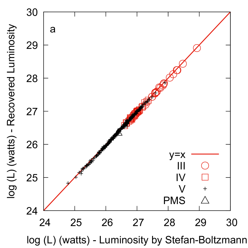
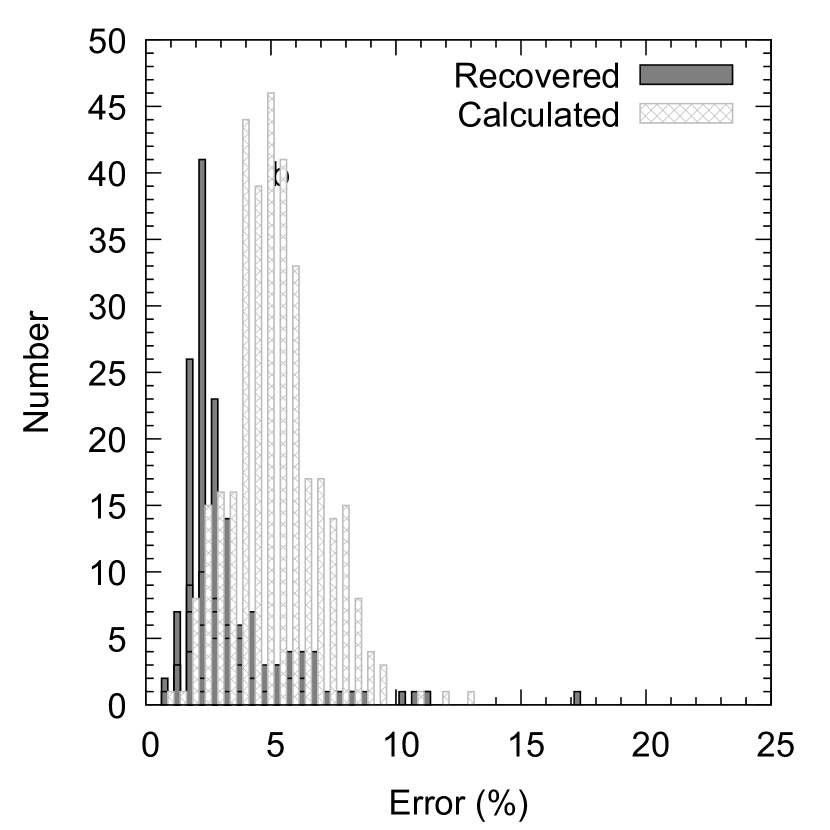
Figure 8: a) Comparing recovered $L$ (from photometry) and calculated $L$ (from $R$ and $T_{\rm eff}$) of the sample stars. b) Histogram distribution of the uncertainties associated with recovered (dark) $L$ is compared to the histogram distribution of the uncertainties associated with calculated (grey) $L$.

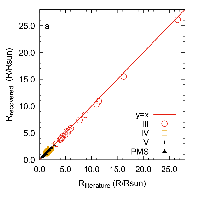
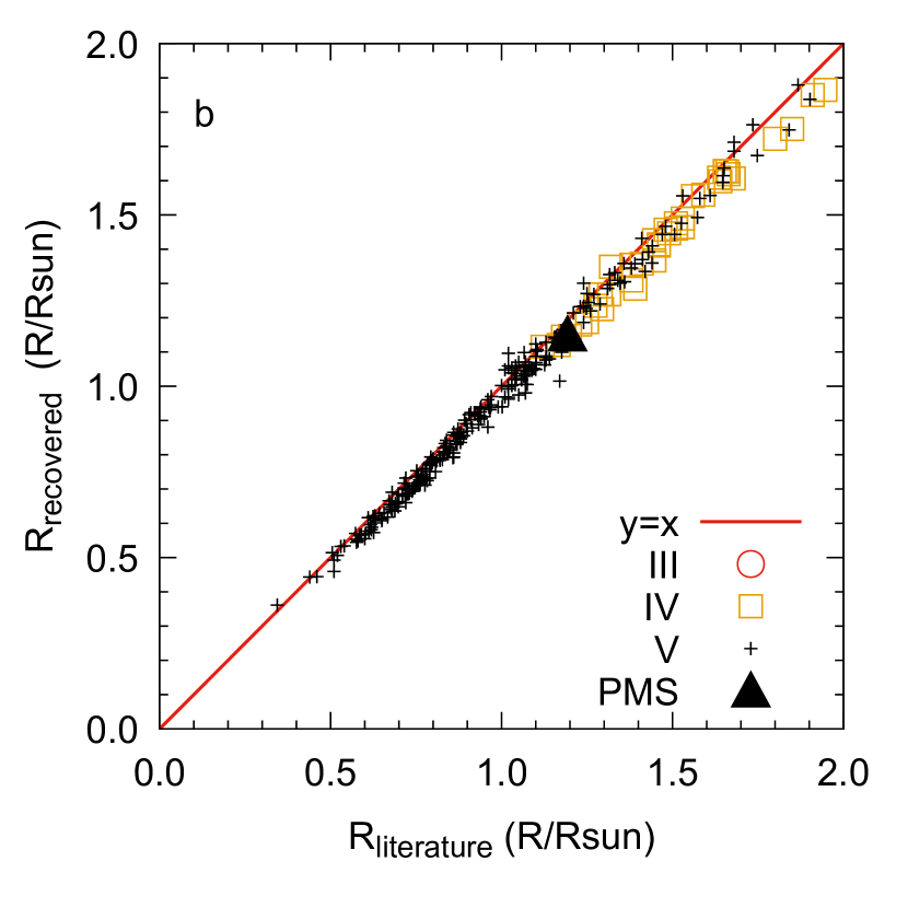
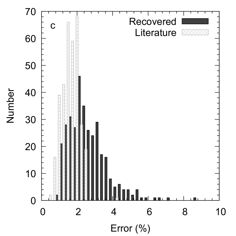
Figure 9: Comparing recovered and published R of giants (a), subgiants (b), main-sequence stars and a PMS star. Error histograms of recovered and published $R$ (c).

4 Discussions

It is known that $BC$ of a star does not only vary by its spectral type and/or $T_{\rm eff}$ but also varies by its luminosity class (log $g$) (Johnson, 1966; Cox, 2000) and metallicity [m/H] (Girardi et al., 2002, 2008; Masana et al., 2006; Pedersen et al., 2020) and even by its rotation speed (Chen et al., 2019). However, the empirical $BC$ values and the $BC-T_{\rm eff}$ relations of Flower (1996), which were rectified later by Torres (2010), was claimed unique for all luminosity classes; main-sequence (V), subgiants (IV), giants (III), supergiants (II) and bright supergiants (I). Unfortunately, being deduced from the 335 stars of mixed luminosity collected from the literature, the data was not sufficient to calibrate various $BC-T_{\rm eff}$ relations of different luminosity classes.

Therefore, the original and the rectified relations were claimed to be valid at all luminosity classes in the temperature range from 2900 to 52000 K which were expressed by three different polynomials each covering a temperature range as log $T_{\rm eff}$ $<$ 3.70, 3.70 $<$ log $T_{\rm eff}$ $<$ 3.90 and log $T_{\rm eff}$ $>$ 3.90 by a note “The $T_{\rm eff}$:$BC$ relation for stars with temperatures less than $\sim$5000 K, however, is uncertain”. Torres (2010) quoted “Many authors find this source convenient because, in addition to the table, it presents simple polynomial fits for $BC_{\rm V}$ valid over a wide range of temperatures.”, therefore, the claim of Flower (1996) is critical to be tested for the sake of $BC$ users in various fields of astrophysics.

Flower (1996) was the only study giving $BC_{\rm V}$ of a star as a function of its $T_{\rm eff}$ while other sources of $BC$ were in tabulated forms until Eker et al. (2020) who calibrated a single main-sequence $BC_{\rm V}-T_{\rm eff}$ relation valid in the temperature range 3100 - 36000 K using the published parameters of 290 DDEB systems having Gaia DR2 trigonometric parallaxes. Non-main-sequence empirical $BC-T_{\rm eff}$ relations are still not calibrated to confirm theoretically claimed differences of a $BC$ at various luminosity classes which appear as the tabulated tables generated theoretically using model atmospheres.

The situation has not yet changed, thus, one way of testing the claim of Flower (1996) is to apply most recently calibrated main-sequence empirical multi-band $BC-T_{\rm eff}$ relations of Bakış & Eker (2022) and $BC_{\rm TESS}-T_{\rm eff}$ relation of this study on the stars with most accurate $R$ and $T_{\rm eff}$ with mixed luminosity classes and to see how successful their $L$ would be recovered from their multiband apparent magnitudes (Johnson $B$, $V$, Gaia $G$, $G_{\rm BP}$, $G_{\rm RP}$ and $TESS$), $BC$ values (Table 2), parallaxes (Table 3) and interstellar extinctions (Table 4).

This study gave us this opportunity to compare the recovered $L$ from multiband photometry and the computed $L$ from published $R$ and $T_{\rm eff}$ by the Stefan Boltzmann law.

4.1 Comparing $L$ from multiband photometry and $L$ from $R$ and $T_{\rm eff}$

Figure 8a compares the standard $L$ of the host stars (Table 6, column 18) recovered from their six band (Johnson $B$, $V$, Gaia $G$, $G_{\rm BP}$, $G_{\rm RP}$ and $TESS$) photometry and $L$ (Table 3, column 15) of the same sample calculated directly from their published $R$ and $T_{\rm eff}$ using the Stefan-Boltzmann law. Regardless to the luminosity classes of the host stars, an outstanding agreement between the predicted and the computed $L$ values is clear.

Accuracy of the recovered $L$ is indicated in Figure 8b, where histogram error distributions of the recovered $L$ of host stars are compared to the histogram error distributions of the computed $L$. It is obviously seen in Figure 8b that the indirect method of obtaining $L$, which requires a pre-computed $BC$, produced twice more accurate standard $L$ than the direct method because the peak of error distribution of the predicted $L$ is 2 per cent while the peak of error distribution of the computed $L$ is 4 per cent. This result, however, is the result of combining independent photometric $M_{\rm Bol}$ values (Table 6) by a weighted average, where the standard error of the weighted mean is propagated as the relative uncertainty ($\Delta L/L$) of the recovered $L$. If single band photometry is used to obtain a single $M_{\rm Bol}$ from $M_{\xi}$ + $BC_{\xi}$, where $\xi$ is one of the bands of Johnson $B$, $V$, Gaia $G$, $G_{\rm BP}$, $G_{\rm RP}$ and $TESS$, the accuracy of the recovered $L$ would have been worse; worse than the errors of computed $L$ which has a peak at 4 per cent.

Because of very accurate apparent magnitudes, parallaxes and a few per cent accuracies in interstellar extinctions (Table 4), the errors of the absolute magnitudes in Table 5 contributed very little with respect to the error contributions of $BC$s that the errors of $M_{\rm Bol}(\xi)$ in Table 6 are just slightly bigger than the corresponding RMS values in Table 2. According to Table 6 the most accurate $M_{\rm Bol}(\xi)$ would have a 0.111 mag uncertainty, which corresponds to 10 per cent error in the recovered $L$ ($\Delta L/L$) according to Eq.12 if single channel photometry is used. If a non-standard $BC$s were used, an additional 10 per cent error further reducing this accuracy would have been inevitable (see Torres, 2010; Eker et al., 2021a, b, 2022), which was the case in earlier applications with various tabulated $BC$ values.

Figure 8 indicates that a main-sequence $BC$ or $BC-T_{\rm eff}$ relation could be used in predicting $L$ of giants, subgiants and even a PMS also without ruling out the fact that $BC$ of a star also depends on its luminosity class (log $g$), metal abundance and even its rotational speed as displayed by many tabulated $BC$s produced theoretically from model atmospheres. This fact becomes more noticeable in the comparison of the predicted $R$ and published $R$ of the host stars in the next subsection.

4.2 Comparing predicted $R$ to published $R$

Figure 9ab compares the predicted $R$ (Table 6, column 20) from published $T_{\rm eff}$ and recovered $L$ to the published $R$ (Table 3, column 6) of the sample host stars. A sufficiently good agreement between the predicted and published $R$ appears supporting Flower (1996) but, on the other hand, a small but clear offset of giants (Fig 9a) and subgiants (Fig 9b) from the diagonal most probably caused by small difference of $BC$ values among different luminosity classes actually disapproves him. The Small difference appears to be negligible so that a user could be satisfied by the recovered R of a giant star using a main-sequence $BC-T_{\rm eff}$ relation, but this does not mean $BC-T_{\rm eff}$ relations of different luminosity classes are the same.

Accuracy of the predicted $R$ of the whole sample is displayed in Figure 9c, where error histograms of the predicted and published $R$ of the host stars are compared. It is obvious in Figure 9c that the peaks of both distributions are about the same at 2 per cent, however, the error distribution of the predicted $R$ has rather a gradually decreasing tail reaching out to 6 per cent while the errors of published $R$ has a sharply ending tail at 2.5 per cent due to the selection criteria of the host stars for this study. More accurate sides of the distributions are also different so that almost half of the most accurate $R$s of the host stars appear to be moved towards the less accurate side because of the less accurate tail of the $L$ errors (see Fig.4).

Such an error distribution of the predicted $R$ is deducible from Eq.14. Noticing that the peak of the error distribution of the predicted $L$ is at 2 per cent (see Fig. 8b) and the peak of the error distribution of the published $T_{\rm eff}$ (See Fig 4a) is about 1 per cent. Plugging these values into Eq.14, one obtains the typical error of predicted $R$ is $\sim 2$ per cent ($\sqrt{5}$). It is obvios that the errors of published $T_{\rm eff}$ dominate. That is, using multiband $BC-T_{\rm eff}$ relations in this study, it is now possible to obtain $R$ of a single star with a relative error twice the relative error of $T_{\rm eff}$.

4.3 How a main-sequence $BC-T_{\rm eff}$ relation works at all luminosity classes?

Main-sequence $BC-T_{\rm eff}$ relations from Table 2 are used in predicting $L$ and $R$ of the host stars. Figures 8 & 9 indicate predictions are successful within the error limits regardless of the luminosity classes (V, IV, III and a PMS) of the host stars. Therefore, one may think the claim of Flower (1996) "All luminosity classes appear to follow a unique $BC$ - $Teff$ relation" would be true. Consequently, a reader would have a question “How do main-sequence $BC-T_{\rm eff}$ relations work in predicting the $L$ and $R$ of a star, which could be a main sequence star, or a subgiant or a giant and even a pre-main-sequence star?”.

This is because the information about the luminosity class of a star is contained mostly in its apparent magnitude rather than its $BC$. Therefore, because the contributions of $BC$s are secondary or negligible in the predictions of $M_{\rm Bol}(\xi)$, which are $M_{\xi}+BC_{\xi}$, one can apparently obtain standard $L$ and $R$ of a single star, which may belong to any luminosity class V, IV, III, or PMS, from its multiband photometry within the error limits set by the propagation of observational random errors and RMS deviations of the $BC-T_{\rm eff}$ relations (Table 2) if the star has a reliable $T_{\rm eff}$ and parallax.

5 Conclusions

The following main-sequence $BC_{\rm TESS}-T_{\rm eff}$ relation, where $X$ = log $T_{\rm eff}$.

$$BC_{\rm TESS}=-318.533+232.298X-55.2916X^{2}+4.27613X^{3}$$ (15)

is calibrated using the published $R$ and $T_{\rm eff}$ of 390 main-sequence stars which are the components of 202 DDEB with TESS apparent magnitudes selected from 209 DDEB. The other five band (Johnson $B$, $V$, Gaia $G$, $G_{\rm BP}$ and $G_{\rm RP}$) $BC-T_{\rm eff}$ relations (Table 2) calibrated by the same DDEB sample are taken from Bakış & Eker (2022). Being different from previously calibrated relations, which are polynomials of the fourth degree, this newly calibrated relation is found to be a third-degree polynomial fitting best to the existing data. The uncertainties of the coefficients and other statistics such as RMS deviations and correlation coefficient ($R^{2}$) are given in Table 2 together with the other statistics of the other five band-relations.

The five-band $BC-T_{\rm eff}$ relations and $BC$ coefficients were already tested by Bakış & Eker (2022) by a successful recovery of $L$ of the main-sequence stars from the same DDEB sample used in the calibrations of these relations. Consequently, Bakış & Eker (2022) concluded that one of the secondary methods of obtaining $L$, which requires a pre-computed $BC$, may provide more accurate $L$ than the classical method relying on the Stefan-Boltzmann law if the information provided by multiband $BC-T_{\rm eff}$ relations are combined. Briefly, various $M_{\rm Bol}$ are calculated first using the $BC$ values from the multiband $BC-T_{\rm eff}$ relation for the given $T_{\rm eff}$ of a star. Then all $M_{\rm Bol}$ values are combined to a mean $M_{\rm Bol}$. Eq.1 is used to obtain $L$ of the star from the mean $M_{\rm Bol}$. Including the $BC_{\rm TESS}-T_{\rm eff}$ relation produced in this study, the six-band (Johnson $B$, $V$, Gaia $G$, $G_{\rm BP}$, $G_{\rm RP}$ and $TESS$) $BC-T_{\rm eff}$ relations, which are deduced from DDEB components, were tested by recovering the $L$ and $R$ of the single host stars with the most accurate published $T_{\rm eff}$ and $R$ similarly.

Both tests (recovering $L$ and recovering $R$) are found successful to conclude that 1) Using multiband $BC-T_{\rm eff}$ relations and $T_{\rm eff}$, one can obtain $L$ of a single star more accurate than the classical direct method of obtaining $L$ relying on the Stefan-Boltzmann law. 2) Accurately predicted $L$ of a single star could be used in predicting its $R$, a critical parameter for exoplanet studies, with reasonable accuracy. The $T_{\rm eff}$ of the star is the only stellar parameter one needs to know to obtain its $L$ and $R$ in addition to its parallax, apparent magnitudes in Johnson $B$, $V$, Gaia $G$, $G_{\rm BP}$, $G_{\rm RP}$ and $TESS$ passband and interstellar extinctions.

Since the present sample contains stars of various luminosity classes (281 main-sequence, 40 subgiants, 19 giants and 1 PMS), we could conclude that not only $L$ and $R$ of the main-sequence but also subgiant, giant and even pre-main sequence stars could be recovered at about 2 per cent uncertainty if the input $T_{\rm eff}$ in the range from 2900 to 38000 K is accurate to have a one per cent uncertainty using the six band $BC-T_{\rm eff}$ relations in Table 2, despite they were calibrated with main-sequence stars.

This result implies that the claim of Flower (1996) "All luminosity classes appear to follow a unique $BC$ - $Teff$ relation" is true, however, it does not rule out the effect of $logg$ of a star on its $BC$. This is because there is a small but clear underestimation with the recovered $R$ of the subgiant and giant hosts according to Figure 9 and perhaps a similar underestimation of recovered $L$ of the same subgiant and giant hosts also exists in Figure 8. These negligible differences may well be caused by small differences in $BC$ values due to different luminosity classes. Thus, we can also conclude that the information about the luminosity class of a star is mostly contained in its apparent magnitude rather than its $BC$. Thus, a main sequence $BC$ or a main-sequence $BC-T_{\rm eff}$ relation could be used in predicting $L$ and $R$ of single stars in all luminosity classes.

We encourage researchers to calculate $BC$ values of a sufficient number of non-main sequence stars and calibrate empirical $BC-T_{\rm eff}$ relation also for giants, subgiants, and PMS in order to see the difference and to confirm the theoretically produced tabulated $BC$s, where the $BC$ values usually presented as functions of luminosity class (log $g$) (Johnson, 1966; Cox, 2000) and metallicity [m/H] (Girardi et al., 2002, 2008; Masana et al., 2006; Pedersen et al., 2020) and even speed of its rotation (Chen et al., 2019).

Data Availability

The data underlying this article are available in the article and in its online supplementary material.

References

- Andersen (1991) Andersen J., 1991, A&ARv, 3, 91
- Andrae et al. (2018) Andrae R., et al., 2018, A&A, 616, A8
- Antoci et al. (2019) Antoci V., et al., 2019, MNRAS, 490, 4040
- Bakış & Eker (2022) Bakış V., Eker Z., 2022, Acta Astron., 72, 195
- Bakış et al. (2022) Bakış V., et al., 2022, New Astron., 93, 101754
- Bessell (1990) Bessell M. S., 1990, PASP, 102, 1181
- Bessell et al. (1998) Bessell M. S., Castelli F., Plez B., 1998, A&A, 333, 231
- Bohn et al. (2021) Bohn A. J., et al., 2021, A&A, 648, A73
- Bressan et al. (2012) Bressan A., Marigo P., Girardi L., Salasnich B., Dal Cero C., Rubele S., Nanni A., 2012, MNRAS, 427, 127
- Casagrande & VandenBerg (2018) Casagrande L., VandenBerg D. A., 2018, MNRAS, 475, 5023
- Chen et al. (2019) Chen Y., et al., 2019, A&A, 632, A105
- Corsaro et al. (2017) Corsaro E., et al., 2017, A&A, 605, A3
- Cox (2000) Cox A. N., 2000, Allen’s astrophysical quantities. (Berlin:Springer)
- Eddington (1926) Eddington A. S., 1926, The Internal Constitution of the Stars. Cambridge: Cambridge University Press
- Eker et al. (2014) Eker Z., Bilir S., Soydugan F., Gökçe E. Y., Soydugan E., Tüysüz M., Şenyüz T., Demircan O., 2014, Publ. Astron. Soc. Australia, 31, e024
- Eker et al. (2015) Eker Z., et al., 2015, AJ, 149, 131
- Eker et al. (2018) Eker Z., et al., 2018, MNRAS, 479, 5491
- Eker et al. (2020) Eker Z., et al., 2020, MNRAS, 496, 3887
- Eker et al. (2021a) Eker Z., Bakış V., Soydugan F., Bilir S., 2021a, MNRAS, 503, 4231
- Eker et al. (2021b) Eker Z., Soydugan F., Bilir S., Bakış V., 2021b, MNRAS, 507, 3583
- Eker et al. (2022) Eker Z., Soydugan F., Bakış V., Bilir S., Steer I., 2022, AJ, 164, 189
- Espinoza & Jordán (2016) Espinoza N., Jordán A., 2016, MNRAS, 457, 3573
- Evans et al. (2018) Evans D. W., et al., 2018, A&A, 616, A4
- Fitzpatrick (1999) Fitzpatrick E. L., 1999, PASP, 111, 63
- Flower (1996) Flower P. J., 1996, ApJ, 469, 355
- Fulton et al. (2017) Fulton B. J., et al., 2017, AJ, 154, 109
- Gabovits (1938) Gabovits J., 1938, Publications of the Tartu Astrofizica Observatory, 30, A3
- Gaia Collaboration et al. (2016) Gaia Collaboration et al., 2016, A&A, 595, A2
- Girardi et al. (2002) Girardi L., Bertelli G., Bressan A., Chiosi C., Groenewegen M. A. T., Marigo P., Salasnich B., Weiss A., 2002, A&A, 391, 195
- Girardi et al. (2008) Girardi L., et al., 2008, PASP, 120, 583
- Günther et al. (2020) Günther M. N., et al., 2020, AJ, 159, 60
- Hertzsprung (1923) Hertzsprung E., 1923, Bull. Astron. Inst. Netherlands, 2, 15
- Johnson (1966) Johnson H. L., 1966, ARA&A, 4, 193
- Kuiper (1938) Kuiper G. P., 1938, ApJ, 88, 429
- Masana et al. (2006) Masana E., Jordi C., Ribas I., 2006, A&A, 450, 735
- Montalto (2022) Montalto M., 2022, arXiv e-prints, p. arXiv:2210.14559
- Pedersen et al. (2020) Pedersen M. G., Escorza A., Pápics P. I., Aerts C., 2020, MNRAS, 495, 2738
- Popper (1959) Popper D. M., 1959, ApJ, 129, 647
- Ricker et al. (2014) Ricker G. R., et al., 2014, in Oschmann Jacobus M. J., Clampin M., Fazio G. G., MacEwen H. A., eds, Society of Photo-Optical Instrumentation Engineers (SPIE) Conference Series Vol. 9143, Space Telescopes and Instrumentation 2014: Optical, Infrared, and Millimeter Wave. p. 914320 (arXiv:1406.0151), doi:10.1117/12.2063489
- Ricker et al. (2015) Ricker G. R., et al., 2015, Journal of Astronomical Telescopes, Instruments, and Systems, 1, 014003
- Russell et al. (1923) Russell H. N., Adams W. S., Joy A. H., 1923, PASP, 35, 189
- Stassun et al. (2017) Stassun K. G., Collins K. A., Gaudi B. S., 2017, AJ, 153, 136
- Stassun et al. (2018) Stassun K. G., et al., 2018, AJ, 156, 102
- Sullivan et al. (2015) Sullivan P. W., et al., 2015, ApJ, 809, 77
- Sung et al. (2013) Sung H., Lim B., Bessell M. S., Kim J. S., Hur H., Chun M.-Y., Park B.-G., 2013, Journal of Korean Astronomical Society, 46, 103
- Torres (2010) Torres G., 2010, AJ, 140, 1158
- Torres et al. (2010) Torres G., Andersen J., Giménez A., 2010, A&ARv, 18, 67
- Wenger et al. (2000) Wenger M., et al., 2000, A&AS, 143, 9