P-NOC: Adversarial CAM Generation for Weakly Supervised Semantic Segmentation

Abstract

To mitigate the necessity for large amounts of supervised segmentation annotation sets, multiple Weakly Supervised Semantic Segmentation (WSSS) strategies have been devised. These will often rely on advanced data and model regularization strategies to instigate the development of useful properties (e.g., prediction completeness and fidelity to semantic boundaries) in segmentation priors, notwithstanding the lack of annotated information. In this work, we first create a strong baseline by analyzing complementary WSSS techniques and regularizing strategies, considering their strengths and limitations. We then propose a new Class-specific Adversarial Erasing strategy, comprising two adversarial CAM generating networks being gradually refined to produce robust semantic segmentation proposals. Empirical results suggest that our approach induces substantial improvement in the effectiveness of the baseline, resulting in a noticeable improvement over both Pascal VOC 2012 and MS COCO 2014 datasets.

1 Introduction

Notwithstanding being one of the most challenging tasks involved, Image Segmentation is a paramount component in any autonomous imagery reading system [3]. Semantic Segmentation consists in correctly associating each pixel of an image or a video to a specific class from a predefined set, and is, to this day, one of the most prominent topics of study in Computer Vision [27], considering its applicability and effectiveness over multiple real-world automation problems from various domains, such as self-driving vehicles [26], autonomous environment surveillance and violence detection [10], vegetation detection through satellite imaging [40] and medical imagery [16].

Approaches based on Convolutional Networks stand out by consistently outscoring classic techniques with great effectiveness across different areas and datasets [6]. However, these require massive amounts of pixel-level annotated information, obtained through extensive human supervision. Considering limited time and cost constraints, these solutions remain inaccessible to many.

To circumvent these limitations, scientists and engineers often recur to Weakly Supervised Semantic Segmentation (WSSS) [31], where “weakly” refers to partially supervised information, or lack thereof. Recent work investigated deriving semantic segmentation maps from saliency maps [17, 21, 11], bounding boxes [14, 30, 19], scribes and points [31], and even image-level labeled annotations [12, 15, 41].

In its most challenging formulation, comprising only image-level information, WSSS is often addressed by employing complex regularization strategies to reinforce useful segmentation properties. Among many, local attention methods [12], saliency-guided methods [38], and Adversarial Erasing (AE) frameworks [15] stand out, entailing impressive mean Intersection over Union (mIoU) across different datasets. However, these methods are often over-optimized for specific conditions or groups, resulting in the creation of knowledge gaps that can be further explored for better solutions.

In this work, we first investigate complementary regularization strategies to construct a strong baseline, maximizing aspects such as prediction completeness, sensitivity to semantic boundaries, and robustness against noisy labeling. We then propose a new Class-Specific Adversarial Erasing strategy, comprising the adversarial training between the generator and a second, not-so-ordinary network (discriminator): the generator must learn class-specific masks that erase all discriminant features presented to the pretrained discriminator. In turn, the discriminator must learn new class-discriminative features. Our setup explores the features available more effectively, resulting in the coarse segmentation priors with higher quality. Finally, we propose an extension of the unsupervised saliency detector C²AM [38], incorporating “hints” of salient regions previously learned. Its pseudo saliency maps are used to devise better pixel affinity maps [2], employed in the refinement of the priors, implying in segmentation proposals with superior quality and competitive mean Intersection over Union (mIoU) results over the Pascal VOC 2012 [8] and MS COCO 2014 [25] datasets.

2 Related Work

WSSS is oftentimes approached as a two-stage process, in which the missing segmentation maps are derived from a weakly supervised dataset, and subsequently used as pseudo maps to train fully-supervised semantic segmentation models. In this setup, coarse segmentation maps (priors) are devised from hints obtained from weak localization methods, such as Class Activation Mapping (CAM) [43], and subsequently refined by Fully Connected Conditional Random Fields (dCRF) [13] and Random Walk (RW) [2], in which uncertain labels are reassigned considering prior confidence, smoothness, and pixel similarity.

Despite greatly improving the precision of the pseudo segmentation maps, refinement methods are strongly influenced by the quality of the seeds. Thus, authors have studied forms to devise more reliable priors by encouraging the emergence of useful segmentation properties, such prediction completeness [35], sensitivity to semantic boundaries [15], and robustness against noisy labeled data [28].

Attention to Local Details

is paramount to reinforce prediction completeness. In this vein, Puzzle-CAM [12] separates the input image $x_{i}$ in four equal pieces $\hat{x}_{i}^{q},\forall q\in[0,4)$, forwards them through a model $f$ and reconstructs the output activation signal ${A^{\text{re}}}^{c}_{i}=\text{merge}_{q}(f^{c}(\hat{x}_{i}^{q}))$, resulting in an information stream highly focused on local details. This “local” stream is used to regularize the main activation signal $A^{c}_{i}=f^{c}(x_{i})$ while the model is trained to predict multi-label class occurrence within samples via both main and local streams, resulting in more complete and homogeneous activation over all parts of the objects of interest.

Saliency Information

is also employed by various weakly supervised strategies, notably improving their effectiveness [4, 29, 33, 18, 21, 11]. To that end, Xie et al. proposed C²AM [38], an unsupervised method that finds a bi-partition of the spatial field that attempts to separate the salient objects from the background. It does so by extracting both low and high level features $A^{k}\in\mathbb{R}^{HW}$ from a pretrained backbone, and feeding them to a disentangling branch $d:\mathbb{R}^{K}\to[0,1]$, such that $d(A)A$ would represent the foreground (fg) features while $(1-d(A))A$ represented the background (bg) ones. Training ensues by optimizing the model to approximate the feature vectors representing the most visually similar patches, while increasing the distance between the fg and bg vectors.

Adversarial Erasing (AE)

methods are commonly employed to solve WSSS tasks. These aim to devise better CAM generating networks by erasing the most discriminative regions during training, forcing them to account for the remaining (ignored) features [22]. Class-Specific Erasing (CSE) [15], for instance, performs AE through an assisted training setup between two models ($f$ and $oc$), in which the first must learn maps that erase all features associated with a specific class, hence reducing its detection by the $oc$. The CAMs learned in this setup become sufficiently accurate to insulate objects of distinct classes, maintaining coarse fidelity to their semantic boundaries.

3 Proposed Approach

In this section, we detail our approach to obtain more robust semantic segmentation priors.

3.1 Combining Complementary Strategies for a Robust Baseline

Figure 1: Comparison of predictions made by a (a) vanilla network, (b) OC-CSE, and (c) Puzzle-CAM.

Given the complex nature of WSSS, in which one must explore underlying cues on data, solutions are often dependent on multiple criteria being met. A single solution is unlikely to provide optimal results for all scenarios (Figure 1): naive models may be insufficient to cover all portions of large objects, while methods that strive for higher completeness (e.g., Puzzle-CAM) may produce superior priors for singleton classes (that seldom co-occur with other classes), while inadvertently confusing objects of different classes in cluttered scenes. Similarly, AE strategies can better segment objects with complex boundary shapes, at the risk of over-expanding to visually similar regions. For more detailed qualitative and quantitative comparisons, see the supplementary materials.

We are thus naturally drawn to investigate whether the combination of complementary strategies could mitigate their individual shortcomings. As our baseline, we combine Puzzle-CAM, OC-CSE, and label smoothing to reinforce the best properties in each approach: high completeness (to cover all class-specific regions), high sensitivity to semantic boundaries and contours, and robustness against labeling noise.

Definition

Let $f$ and $oc$ be two architecture-sharing CNNs, $x_{i}$ be the $i$-th sample image in the training set, associated with the label vector $y_{i}\in\{0,1\}^{C}$ (indicating the occurrence of at least one object associated to each one of the $C$ existing classes), and $r$ a class randomly drawn from $y_{i}$. We define $A_{i}^{c}=f^{c}(x_{i})\in\mathbb{R}^{HW}$, the $c$-th spatial activation map produced from $x_{i}$ and associated to class $c$, ${A^{\text{re}}}^{c}_{i}=\text{merge}(f^{c}(\text{tile}(x_{i})))$ the reconstruction of the Puzzle-CAM pieces, which were produced by separating $x_{i}$ into four quadrants and forwarding them individually through $f$, and ${A^{\text{oc}}}^{c}_{i}=oc^{c}(x_{i}\circ(1-\psi(A_{i}^{r})))$, the activation map produced when the masked input is forwarded through $oc$.

From the spatial maps, we obtain the estimated posterior probability of $x_{i}$ containing objects of class $c$: $p_{i}^{c}(A)=\sigma(\operatorname{GAP}(A_{i}^{c}))$, ${p^{\text{re}}}^{c}_{i}=\sigma(\operatorname{GAP}({A^{\text{re}}}^{c}_{i}))$ and ${p^{\text{oc}}}^{c}_{i}=\sigma(\operatorname{GAP}({A^{\text{oc}}}^{c}_{i}))$. Finally, we define P-OC as the optimization of the following objective functions:

$$\begin{split}\mathcal{L}_{\text{P-OC}}&=\mathcal{L}_{\text{P}}+\mathcal{L}_{\text{cse}}=(\mathcal{L}_{\text{cls}}+\mathcal{L}_{\text{re-cls}}+\mathcal{L}_{\text{re}})+\mathcal{L}_{\text{cse}}\\ &=\ell_{\text{cls}}(p_{i},y_{i})+\ell_{\text{cls}}(p^{\text{re}}_{i},y_{i})+\lambda_{\text{re}}\|A_{i}-A^{\text{re}}_{i}\|_{1}+\lambda_{\text{cse}}\ell_{\text{cls}}(p_{i}^{\text{oc}},y_{i}\setminus\{r\})\end{split}$$ (1)

where $\ell_{\text{cls}}$ is the multi-label soft margin loss, and $\|\cdot\|_{1}$ the mean absolute error loss.

3.2 Adversarial CAM Generating Learning

The Class-Specific Erasing (CSE) framework [15] has shown great promise among the AE methods, noticeably improving WSSS score compared to previous class-agnostic strategies. When employing an ordinary classifier ($oc$), remaining regions (not erased) associated with a specific class can be quantified, allowing us to better modulate training (a fundamental step in reducing the chronic problem of over-erasure existing in AE methods [22]).

However, it is unlikely that the $oc$ can continue to provide useful information regarding the remaining regions once considerable erasure is performed, as (a) the soft masking from a CAM (devised from a non-saturating linear function) can never fully erase the primary features, and (b) the $oc$ has only been trained over whole images, in which marginal regions could be easily ignored. This behavior is best observed in Figure 2: after many training iterations under the CSE framework, the $oc$ remains focused on core regions of the class horse, notwithstanding these been mostly erased. Once the input is hard masked, completely removing these regions, the $oc$ can focus on secondary regions (the horses’ legs), and thus provide better information about which regions are ignored by $f$.

Figure 2: Diagram of an adversarial learning scheme. OC: class-specific regions are erased (CSE) with the supervision of a fixed ordinary classifier ($oc$). After many training iterations, core regions associated with a class are saturated, rendering the $oc$ redundant. NOC: a not-so-ordinary classifier ($noc$) is gradually trained to associate secondary, (and yet) discriminant regions to the class of interest.

Method

To overcome this limitation, we propose to extend the CSE framework into a fully adversarial training one (namely P-NOC). In it, the generator $f$ must learn class activation maps that erase all regions that contribute to the classification of class $r$, while a second network $noc$ (a “not-so-ordinary” classifier) must discriminate the remaining $r$-specific regions neglected by $f$, while learning new features that characterize $r$, currently ignored by both. In summary, P-NOC is trained by alternatively optimizing two objectives:

$$\mathcal{L}_{f} =\mathbb{E}_{(x,y)\sim\mathcal{D},r\sim y}[\mathcal{L}_{\text{P}}+\lambda_{\text{cse}}\ell_{\text{cls}}(p^{\text{oc}},y\setminus\{r\})]$$ (2)

$$\mathcal{L}_{\text{noc}} =\mathbb{E}_{(x,y)\sim\mathcal{D},r\sim y}[\lambda_{\text{noc}}\ell_{\text{cls}}(p^{\text{noc}},y)]$$ (3)

where $p^{\text{noc}}=oc(x\circ(1-\psi(A^{r})>\delta_{\text{noc}}))$.

We reuse P-OC as our generator to retain the properties discussed in Section 3.1, and employ a $\lambda_{noc}$ weight factor to avoid a premature (and late) corruption of internalized knowledge of $noc$ (see Section 4 for details).

By refining $noc$ to match the masked image to the label vector $y$, in which $y^{r}=1$, we expect it to gradually shift its attention towards secondary (and yet discriminative) regions, and, thus, to provide more useful regularization to the training of the generator. Concomitantly, we expect $f$ to not forget the class discriminative regions learned so far, considering (a) its learning rate is linearly decaying towards $0$; and (b) the degeneration of the masks would result in an increase of $\mathcal{L}_{\text{cse}}$. Figure 3 illustrates all elements and objectives confined in our strategy, and a pseudocode of P-NOC is provided in Algorithm 1.

Figure 3: Overview of the objectives in the P-NOC training setup. In each training step, a sample $x_{i}$ is presented to $f$, which is optimized to produce attention maps considering the regularization provided by both Puzzle module and a “not-so-ordinary” classifier $noc$. Sub-sequentially, $f$ is fixed and $noc$ is refined to shift its attention to useful regions, currently neglected by both networks.

Algorithm 1 Proposed P-NOC algorithm

1:Training set $\mathcal{D}=\{\mathcal{X},\mathcal{Y}\}$, CAM generating networks $f$ and $noc$, $k_{noc}\in\mathbb{N}$, $\delta_{\text{noc}}\in(0,1)$

2:

3:while not done do

4:    Sample a batch $(x_{i},y_{i})$ from $\mathcal{D}$, and $r$ from $y_{i}$

5:    // Fix $noc$ and train $f$

6:    Compute $A^{c}_{i}=f(x_{i}),{A^{\text{re}}}^{c}_{i}=\text{merge}(f(\text{tile}(x_{i})))$

7:    Compute $\mathcal{L}_{\text{P-OC}}$ loss from Eq. 2

8:    Update weights of $f$ by $\nabla\mathcal{L}_{\text{P-OC}}$

9:    if $i\mod k_{noc}=0$ then

10:         // Fix $f$ and train $noc$

11:         $\hat{x}_{i}=x_{i}\circ(1-\psi(A^{r}_{i})>\delta_{\text{noc}})$

12:         Compute $\mathcal{L}_{noc}$ from Eq. 3

13:         Update weights of $noc$ by $\nabla\mathcal{L}_{\text{noc}}$

14:    end if

15:end while

3.3 Deriving Saliency Maps from Weakly Supervised Information

The utilization of saliency information as complementary information is unequivocally advantageous for the solution of WSSS tasks. Many studies conducted thus far focus on the utilization of saliency hints (advent from pretrained saliency detectors) to improve segmentation precision, but neglect the underlying risk of data leakage: when these detectors been pretrained over datasets containing elements (samples, classes, context) that intersect the current segmentation task. C²AM [38] addresses this risk by employing an unsupervised saliency detection approach.

C²AM

Let $P^{hw}:\mathbb{R}^{hw}\to[0,1]^{chw}$ be a function mapping each region in the embedded spatial signal $A_{i}^{hw}$ to the probability value $p_{i}^{hw}$ of said region belonging to the first partition. Moreover, let $v_{i}^{f}=P_{i}\circ A_{i}$ and $v_{i}^{b}=(1-P_{i})\circ A_{i}$ be two extracted feature vectors, representing the spatial foreground (fg) and background (bg) features, respectively. Considering a batch of $n$ images $\mathcal{B}=\{x_{b},x_{b+1},\ldots,x_{b+n-1}\}$, three cosine similarity matrices are calculated: (a) the fg features ($s^{f}_{ij}$), (b) the bg features ($s^{b}_{ij}$); and (c) between the fg and bg ($s^{\text{neg}}_{ij}$) features. In these conditions, C²AM [38] is defined as the optimization of the objectives:

$$\begin{split}\mathcal{L}^{\mathcal{B}}_{\text{C²AM}}&=\mathcal{L}^{\mathcal{B}}_{\text{pos-f}}+\mathcal{L}^{\mathcal{B}}_{\text{pos-b}}+\mathcal{L}^{\mathcal{B}}_{\text{neg}}\\ &=\frac{1}{n(n-1)}\sum_{i}^{n}\sum_{j}^{n}\mathds{1}_{[i\neq j]}(w^{f}_{ij}\log s^{f}_{ij})+\frac{1}{n(n-1)}\sum_{i}^{n}\sum_{j}^{n}\mathds{1}_{[i\neq j]}(w^{b}_{ij}\log s^{b}_{ij})\\ &-\frac{1}{n^{2}}\sum_{i}\sum_{j}\log(1-s^{\text{neg}}_{ij})\end{split}$$ (4)

where $w^{f}_{ij}$ and $w^{b}_{ij}$ are exponentially proportional to the similarity rank between the regions $(i,j)$, considering all possible pairs available in $A_{b}$ ($w_{ij}=e^{-\alpha\text{rank}(s_{ij})},w\in\{w^{f},w^{b}\}$).

Of course, C²AM is not without shortcomings. With careful inspection of Eq. 4, it is noticeable the absence of an “anchor”: similar pixels representative of salient objects (relative to the dataset of interest) can either be associated with low or high values in $P^{hw}$. I.e., C²AM establishes a bi-partition of the visual receptive field, without specifying which partition contains salient objects. Furthermore, no explicit reinforcement is made to create a bi-partition that aggregates all salient classes in the set. Instead, similar regions are simply projected together, implying in the risk of salient objects of different classes to be placed in different partitions. For example, in extreme scenarios, where two classes never appear spatially close to each other, or indirectly through an intermediate class.

Finally, C²AM considers similarity based on low and high level features from a pretrained model, which may differ from the semantic boundaries of classes in the problem at hand. It stands to reason that additional inductive bias, related to the segmentation of the task at hand, may benefit the learning of a better bi-partition function by C²AM.

Method

We propose to utilize saliency hints, extracted from models trained in the weakly supervised scheme, to further enrich the training of C²AM. Our approach is inspired by recently obtained results in the task of Semi-Supervised Semantic Segmentation, in which a teacher network is used to regularize the training of a student network [36].

For every image $x_{i}$, saliency hints can be retrieved by thresholding the maximum pixel activation in its CAM by a foreground constant ($\max_{c}\psi(A_{i}^{c})>\delta_{\text{fg}}$), resulting in a map that highlights regions that likely contain salient objects. Given the previously observed lack of completeness in CAMs, only regions associated with a high activation intensity are considered as fg hints, and thus used to reinforce a strong output classification value for the disentangling branch $d$. Regions associated with a low activation intensity are discarded.

Figure 4(a) illustrates examples of CAMs, background and foreground hints extracted from RS269 P-OC network. We notice fg hints tend to be significantly accurate (rarely activating over background regions). Conversely, background hints are less accurate, often highlighting salient objects due to the lack of prediction completeness.

We define C²AM-H as an extension of C²AM, in which fg hints are employed to guide training towards a solution in which salient regions are associated with high prediction values from $d$ (anchored), and all salient objects are contained within the same partition. In practice, this implies in the addition of a new objective function in Eq. 4: the cross-entropy loss term between the collected hints $\hat{y}_{i}$, for $i\in[b,b+n)$ and the posterior probability predicted by $d$. I.e., C²AM-H is trained with the following multi-objective loss:

$$\mathcal{L}^{\mathcal{B}}_{\text{C²AM-H}}=\mathcal{L}^{\mathcal{B}}_{\text{pos-f}}+\mathcal{L}^{\mathcal{B}}_{\text{pos-b}}+\mathcal{L}^{\mathcal{B}}_{\text{neg}}+\lambda_{h}\sum_{i\in b}\sum_{h,w}\mathds{1}_{[A_{i}^{hw}>\delta_{\text{fg}}]}\ell_{\text{cls}}(\hat{y}^{hw}_{i},p^{hw}_{i})$$ (5)

where $\mathds{1}_{[A_{i}^{hw}>\delta_{\text{fg}}]}$ is a mask applied to ensure only regions associated with a normalized activation intensity higher than $\delta_{\text{fg}}$ are considered as foreground hints.

Figure 4(b) illustrates examples of saliency masks obtained by a simple saliency detection network, when trained over pseudo masks devised from C²AM-H. Fidelity to semantic boundaries are noticeably in these examples.

(a)

(b)

Figure 4: (a) Example of hints extracted with the RS269 P-OC network. From top to bottom: (i) the CAMs; (ii) background hints: regions where activation is below $\delta_{\text{bg}}=0.1$; and (iii) foreground hints: regions where activation intensity is higher than $\delta_{\text{fg}}=0.4$. (b) Saliency maps from a simple saliency detector, trained over priors devised from C²AM-H (hints from P-NOC+LS).

3.3.1 Guiding Random Walk using Saliency Maps

Originally, affinity maps are devised by employing two thresholds ($\delta_{bg}$ and $\delta_{fg}$) over the prior maps to determine core regions (likely depicting bg or fg regions, respectively). Regions whose saliency both maps cannot agree upon are marked as uncertain, and ignored when training the affinity function.

We propose a slight modification to this procedure to incorporates the saliency maps obtained from C²AM-H: we assign the background label to pixels whose saliency value are low; a class label for pixels with a strong CAM signal for that specific class, and the uncertain label for pixels with strong saliency value and weak CAM signal. Affinity maps devised this way are less prone to the problem of prediction completeness and more semantic boundary aware, resulting in (a) less false negative pixels (fg regions labels as bg), (b) smaller uncertain regions, and (c) faithful semantic boundaries. This is best seen in the last column of Figure 5.

We further remark that this strategy yields more affinity pairs when training the pixel-wise affinity function [2], as well as harder case pairs, closer to the semantic boundaries of the salient objects.

Figure 5: Comparison between the different affinity maps obtained from RS269 trained with P-OC+LS. From left to right: (a) images and ground-truth segmentation; (b) affinity labels devised from priors; (c) affinity labels refined with dCRF; and (d) affinity labels obtained using both C²AM-H and dCRF.

4 Experimental Setup

In accordance with literature [2, 15, 12], CAM-generating models are trained with Stochastic Gradient Descent (SGD) for $15$ epochs with linearly decaying learning rates of $0.1$ and $0.01$ (for randomly initialized weights and pre-trained weights, respectively), and $1\text{e-4}$ weight decay. Furthermore, samples are augmented with random resizing/cropping, while label smoothing [34, 28] is applied. To improve classification robustness, we employ RandAugment (RA) [7] when training Ordinary Classifiers. Conversely, we observed a marginal decrease in mIoU when training Puzzle and OC-CSE models with RA, and thus opted to train them with simple color augmentation (variation of contrast, brightness, saturation, and hue). When training P-OC, the coefficients $\lambda_{\text{re}}$ and $\lambda_{\text{cse}}$ are kept as originally proposed: $\lambda_{\text{re}}$ increases linearly from $0$ to $4$ during the first half epochs, while $\lambda_{\text{cse}}$ increases linearly from $0.3$ to $1$ throughout training. For P-NOC, $\lambda_{\text{noc}}$ increases from $0$ to $1$, while learning rate decreases from its initial value to $0$. These settings constraint $oc$ to change more significantly in the intermediate epochs, and, thus, to recognize prominent regions of objects in the first stages of training, while preventing it from learning incorrect features later on. We set $\sigma_{\text{noc}}=0.2$ following previous work.

C²AM and C²AM-H are trained with the same hyperparameters as Xie et al. [38], except for the batch size, which is set to 32 for the ResNeSt269 architecture due to hardware limitations. For C²AM-H, we set $\delta_{fg}=0.4$ and $\lambda_{h}=1$ after inspecting samples for each class, and confirming a low false positive rate for foreground regions in the limited inspection subset. We leave the search for their optimal values as future work.

In accordance with the baseline [12], we employ DeepLabV3+ [5] as segmentation network and train it over the pseudo masks obtained in the previous stage. We maintain the training setup unchanged, except for the employment of label smoothing.

4.1 Note on Puzzle’s Fairness

Upon closer inspection over Puzzle-CAM’s training loop, it becomes evident the existence of an early stopping mechanism that persists the weights of the model as training progresses, conditioned to the improvement of the metric of interest (mIoU). Hence, privileged and fully-supervised information (advent from the ground-truth maps) is being incorporated in the training procedure, further fortifying it against overfit, albeit mischaracterizing a supposedly weakly-supervised problem. We further remark that many of the WSSS studies conducted so far [15, 2, 17, 21] have not employed similar early stopping mechanisms, implying that the comparison between them and Puzzle-CAM is not straight-forward. Therefore, the results reported by Jo and Yu [12] do not represent the expected effectiveness of Puzzle-CAM, when applied over truly WSSS problems. They may be nevertheless interpreted as an estimate for its potential effectiveness, reached if some information is available to guide the validation process, or if mIoU is coincidentally at its highest on the last iteration.

To provide a fairer comparison with literature and more reliable evaluation of the approach, we re-implement and evaluate Puzzle-CAM without the aforementioned mechanism. For the remaining of this work, we refer to our “fair” re-implementation as Puzzle^f (or P^f).

5 Results

Table 1: The mIoU (%) values measured in each epoch over Pascal VOC 2012 train set, considering the architectures ResNet50 (RN5), ResNeSt101 (RS101) and ResNeSt269 (RS269); and training strategies RandAugment (RA), Puzzle (P^f), and Puzzle-OC (P-OC). Scores averaged among three runs.

Strategy	E1	E2	E3	E4	E5	E6	E7	E8	E9	E10	E11	E12	E13	E14	E15	TTA
RS101 RA	48.7	48.2	50.5	50.4	49.1	49.5	49.2	49.8	41.0	48.9	48.7	49.4	48.9	49.2	49.2	54.8
RS269 RA	47.3	49.0	49.3	49.2	49.2	48.8	48.7	48.7	48.6	48.7	48.7	48.2	48.0	48.1	48.1	53.9
RS101 Pf	50.4	51.4	53.2	53.4	52.5	52.9	54.0	54.7	54.2	51.8	53.8	54.7	54.2	54.6	54.9	59.4
RS269 Pf	50.4	52.5	54.3	53.9	55.5	55.9	55.4	56.1	56.3	57.0	55.6	56.7	55.2	56.7	56.2	60.9
RS101 P-OC	49.6	50.3	51.5	51.8	52.5	51.5	49.0	49.9	53.2	52.5	53.4	54.2	54.9	55.5	56.0	59.1
RS269 P-OC	49.0	51.1	52.6	53.6	54.1	53.8	51.9	54.8	55.2	55.7	54.1	55.6	57.0	57.0	57.4	61.4
RS269 P-OC+LS	50.6	52.5	53.5	54.3	53.9	55.0	55.2	55.3	56.4	56.1	55.8	56.2	55.9	57.5	58.5	61.8
RS269 P-NOC+LS	49.0	51.6	53.0	53.9	55.5	55.5	55.8	56.4	57.2	58.3	56.9	58.9	58.8	58.9	59.2	63.6

Priors

Table 1 illustrates mIoU measured at the end of each training epoch, considering various architectures and training strategies. For performance purposes, samples are resized to a common frame, and Test-Time Augmentation (TTA) is not employed. Thus, the intermediate measurements are estimations of the true scores (represented in the column E15). RandAugment (RA) and Puzzle (P^f) present saturation on early epochs, and a significant deterioration in mIoU for the following ones. On the other hand, Combining Puzzle and OC-CSE (P-OC) induces a notable increase in mIoU for all architectures, with a score peak on latter epochs. On average, P-OC obtains 61.44% mIoU when TTA is used, lower than the original Puzzle (62.04%), but 0.55 percent point above P^f (60.89%). Applying label smoothing to P-OC (P-OC+LS) improves TTA score by 0.34 p.p. (61.77%). Finally, employing the adversarial training of $noc$ (P-NOC+LS) results in 63.66% mIoU (1.89 p.p. improvement).

Ablation Studies

Table 2 describes the mIoU scores obtained throughout the different stages of training. The utilization of saliency maps (P-OC C²AM-H) increases the mIoU of the pseudo segmentation maps by 0.40 p.p. Finally, training $noc$ (+NOC) reduces improves mIoU by 2.22 p.p and 1.58 p.p over training and validation subsets, respectively.

Table 2: Ablation studies of pseudo segmentation maps produced by RW over priors, measured in mIoU (%) over VOC12 train and val sets.

Method	+LS	+C²AM-H	+NOC	Train	Val
Pf				71.35	70.67
P-OC				73.50	72.08
P-OC	✓			71.45	70.15
P-OC		✓		73.90	72.53
P-OC	✓	✓		73.07	72.14
P-OC	✓		✓	73.31	72.83
P-OC	✓	✓	✓	75.53	74.41

Figure 6: Segmentation results by DeepLabV3+, trained with priors obtained from P-NOC and refined with C²AM-H and RW.

5.0.1 Weakly Supervised Saliency Detection (C²AM-H)

Table 3: The ablation study for C²AM-H. Measured mIoU over VOC12 training set. Scores are reported in mIoU (%), considering both priors (P.) and maps refined with PoolNet (R.).

Method	B.bone	Hints	Segm. Priors	P.	R.
C²AM	RN50	-	RN50 P	56.6	65.5
C²AM	RN50	-	RS269 Pf	59.1	65.3
C²AM	RN50	-	RS269 P-OC	60.8	67.3
C²AM	RN50	-	RS269 P-OC+LS	61.2	67.2
C²AM	RN50	-	GT	63.4	65.0
C²AM	RS269	-	GT	61.4	-
C²AM-H	RN50	RS269 P-OC	GT	64.8	-
C²AM-H	RS101	RS269 P-OC	GT	69.6	-
C²AM-H	RS269	RS269 P-OC	GT	69.9	70.9
C²AM-H	RS269	RS269 P-OC+LS	GT	70.3	71.7
C²AM-H	RS269	RS269 P-NOC+LS	GT	70.6	72.4
C²AM-H	RS269	RS269 P-OC	RS101 RA	66.5	66.2
C²AM-H	RS269	RS269 P-OC	RS101 P-OC	66.7	67.9
C²AM-H	RS269	RS269 P-OC	RS269 P-OC	66.8	68.6
C²AM-H	RS269	RS269 P-OC	RS269 P-OC+LS	67.3	68.8
C²AM-H	RS269	RS269 P-OC+LS	RS269 P-OC+LS	67.3	69.2
C²AM-H	RS269	RS269 P-OC+LS	RS269 P-NOC+LS	67.7	70.6
C²AM-H	RS269	RS269 P-NOC+LS	RS269 P-NOC+LS	67.9	70.8

In conformity with literature [38], we evaluate the effectiveness of C²AM-H by combining the devised saliency maps with the semantic priors and measuring the resulting mIoU scores over the dataset. Table 3 displays the scores obtained when combining semantic segmentation priors with saliency maps produced by the C²AM (baseline) and C²AM-H (trained with additional fg hints). Firstly, employing priors devised from P-OC (third and fourth row) substantially improves mIoU, when compared to the baseline and RS269 trained with Puzzle^f (first and second rows, respectively).

To isolate the contribution of the saliency maps to the score, we also evaluate models using the ground-truth semantic segmentation annotations (GT) as priors. That is, the prediction for a given pixel in the image will be considered correct if that pixel was predicted as salient, and it is annotated with class $c$. Conversely, a pixel annotated with $c$ and predicted as non-salient (or annotated as bg and predicted as salient) is considered a miss. In this evaluation setup, the baseline (C²AM RN50) scored 65.03% mIoU, while the best strategy (C²AM-H, using hints from RS269 P-OC+LS) achieves 71.70% mIoU (a 6.67 p.p. increase).

Replacing the architecture of C²AM (C²AM RS269), or using hints to train the RN50 architecture (C²AM-H RN50) have produced mixed results: a 2.02 percent point score reduction for the former, and a 1.39 percent point score increase for the latter. We hypothesize this has occurred due to a representation deficit created when training with a reduced batch size, and to an inability of the RN50 architecture to produce more detailed saliency maps, rendering the additional regularization provided by hints useless. Finally, our best strategy (priors and hints from P-OC_+LS) scores 69.22% mIoU, with only a marginal difference to P-NOC, indicating that its score gain were normalized with the employment of saliency.

A comparison with the State of the Art is shown in Table 5. Training a segmentation model over the pseudo masks obtained from P-OC+C²AM-H results in a solution with 71.38% and 72.35% mIoU scores over the VOC12 val and test set, respectively, slightly outscoring the “unfair” version of Puzzle-CAM in the test set, and the remaining approaches by a considerable margin. Moreover, training over masks obtained from P-NOC+LS+C²AM-H results in the best solution, with 73.46% test mIoU. A few examples of predicted masks are illustrated in Figure 6, while class-specific IoU scores are shown in Table 6.

Table 4: Comparison with SOTA methods on Pascal VOC 2012, measured in mIoU (%). Puzzle-CAM: potential effectiveness reported (see Section 4.1).

Method	Backbone	Val	Test
AffinityNet [2]	W-ResNet-38	61.7	63.7
ICD [9]	ResNet-101	64.1	64.3
IRNet [1]	ResNet-50	63.5	64.8
SEAM [37]	W-ResNet-38	64.5	65.7
OC-CSE [15]	W-ResNet-38	68.4	68.2
RIB [17]	ResNet-101	68.3	68.6
AMN [20]	ResNet-101	69.5	69.6
EPS [21]	ResNet-101	70.9	70.8
ViT-PCM [32]	ViT-B/16	70.3	70.9
MCT-Former [39]	W-ResNet-38	71.9	71.6
Puzzle-CAM [12]	ResNeSt-269	71.9	72.2
P-OC+C²AM-H (ours)	ResNeSt-269	71.4	72.4
P-NOC+LS+C²AM-H (ours)	ResNeSt-269	73.6	73.5

Table 5: Comparison with SOTA methods on MS COCO 2014 datasets, measured in mIoU (%). $\dagger$: employment of additional (saliency) annotations.

Method	Backbone	Val
IRNet [1]	ResNet-50	32.6
IRN+CONTA [42]	ResNet-50	33.4
EPS† [21]	ResNet-101	35.7
OC-CSE [15]	W-ResNet-38	36.4
PPM [24]	ScaleNet	40.2
URN [23]	ResNet-101	40.7
MCT-Former [39]	W-ResNet-38	42.0
RIB [17]	ResNet-101	43.8
IRN+AMN [20]	ResNet-101	44.7
ViT-PCM [32]	ViT-B/16	45.0
P-NOC+C²AM-H (ours)	ResNeSt-269	47.7

Following the literature, we evaluate P-NOC over the more challenging MS COCO 2014 dataset, and present the results in Table 5. Our approach achieves 47.74% mIoU, outperforming OC-CSE and more recent WSSS methods. We attribute this noticeable improvement (relative to the modest one observed in Pascal VOC 2012) to the nature of this set, in which multiple (and more) objects of different classes frequently co-exist in the same scenarios.

Table 6: Intersection over Union (IoU %) obtained by segmentation models over the Pascal VOC 2012 test set, after being trained over pseudo segmentation masks devised from P-OC and P-NOC.

	bg	plane	bike	bird	boat	bottle	bus	car	cat	chair	cow	table	dog	horse	mbk.	person	plant	sheep	sofa	train	tv	avg.
AffinityNet	88.2	68.2	30.6	81.1	49.6	61.0	77.8	66.1	75.1	29.0	66.0	40.2	80.4	62.0	70.4	73.7	42.5	70.7	42.6	68.1	51.6	61.7
OC-CSE	90.2	82.9	35.1	86.8	59.4	70.6	82.5	78.1	87.4	30.1	79.4	45.9	83.1	83.4	75.7	73.4	48.1	89.3	42.7	60.4	52.3	68.4
AMN	90.7	82.8	32.4	84.8	59.4	70.0	86.7	83.0	86.9	30.1	79.2	56.6	83.0	81.9	78.3	72.7	52.9	81.4	59.8	53.1	56.4	69.6
ViT-PCM	91.1	88.9	39.0	87.0	58.8	69.4	89.4	85.4	89.9	30.7	82.6	62.2	85.7	83.6	79.7	81.6	52.1	82.0	26.5	80.3	42.4	70.9
MCT-Former	92.3	84.4	37.2	82.8	60.0	72.8	78.0	79.0	89.4	31.7	84.5	59.1	85.3	83.8	79.2	81.0	53.9	85.3	60.5	65.7	57.7	71.6
P-OC (ours)	91.6	86.7	38.3	89.3	61.1	74.8	92.0	86.6	89.9	20.5	85.8	57.0	90.2	83.5	83.4	80.8	68.0	87.0	47.1	62.8	43.1	72.4
P-NOC (ours)	91.7	87.9	38.1	80.9	66.1	69.8	93.8	86.4	93.2	37.4	83.6	60.9	92.3	84.7	83.8	80.5	62.3	81.9	53.1	77.7	36.7	73.5

6 Conclusions

In this work, we first investigated complementary regularization methods to construct a strong baseline, considering properties such as completeness and sensitivity to semantic contours of objects. We proposed the adversarial training of CAM generating networks to mitigate the attention deficit to marginal features observed in the Class-Specific Adversarial framework. Finally, we proposed C²AM-H, an extension of C²AM that incorporates hints of salient regions to devise more robust salient maps in a weakly supervised fashion. Our empirical results suggest that these interventions provide noticeable improvement in all stages, resulting in solutions that are both more effective and robust against data noise.

As future work, we will study the effect of strong augmentation (e.g., MixUp, ClassMix, and CowMix) in WSSS; evaluate our approach over functional segmentation problems and instance segmentation problems; and devise forms to reduce computational footprint.

Appendix A Supplementary Materials

A.1 Additional Training and Evaluation Details

A.1.1 Semantic Segmentation Priors

Following previous work [2, 15, 12], CAM-generating models are trained over the Pascal VOC 2012 dataset [8] with Stochastic Gradient Descent (SGD) for $15$ epochs with linearly decaying learning rates of $0.1$ and $0.01$ (for randomly initialized weights and pre-trained weights, respectively), and $1\text{e-4}$ weight decay. We set a batch size of 32 for all architectures but ResNeSt-269, due to hardware limitations. The latter is trained with a batch of 16 samples in the Puzzle-CAM, P-OC and P-NOC training setups, and gradients are accumulated on each odd step, and only applied on even steps. For the MS COCO 2014 dataset [25], models are trained with learning rates $0.05$ and $0.005$ for randomly initialized weights and pre-trained weights, respectively.

During training, an image sample is resized by a random factor ranging between 0.5 to 2.0, with a patch of 512 per 512 pixels² being subsequently extracted from a random position. RandAugment (RA) [7] is utilized when training vanilla models, which will later be employed as Ordinary Classifiers (OCs), to induce a higher classification effectiveness and robustness against data noise. We only employ weak image augmentation procedures (changes in image brightness, contrast, and hue) when training Puzzle-CAM, P-OC and P-NOC. Label Smoothing [34, 28] is applied to the P-OC and P-NOC training strategies.

Three different models are trained for each strategy, with their training history being illustrated in Table 7. Test-Time Augmentation (TTA) is employed to produce the final segmentation priors: images are resized according to the factors 0.5, 1.0, 1.5 and 2.0, and are sequentially fed (along with their horizontal reflection) to the model, producing 8 different CAMs, which are subsequently averaged to create the segmentation prior.

P-OC. When training (P-OC), the coefficients $\lambda_{\text{re}}$ and $\lambda_{\text{cse}}$ are kept as originally proposed: $\lambda_{\text{re}}$ increases linearly from $0$ to $4$ during the first half epochs, while $\lambda_{\text{cse}}$ increases linearly from $0.3$ to $1$ throughout training.

P-NOC. The factor $\lambda_{\text{noc}}$ increases from $0$ to $1$, while learning rate decreases from its initial value to $0$. These settings constraint $noc$ to change more significantly in the intermediate epochs, and, thus, to recognize prominent regions of objects in the first stages of training, while preventing it from learning incorrect features later on. Figure 7 (a) illustrates the change in the effective learning rate of $noc$ over time.

A.1.2 Deriving Saliency Maps from Weakly Supervised Information

C²AM and C²AM-H are trained with the same hyperparameters as Xie et al. [38], except for the batch size, which is set to 32 for the ResNeSt269 architecture due to hardware limitations. When training C²AM-H, we set $\delta_{\text{fg}}$ and $\lambda_{h}$ to $0.4$ and $1$, respectively. These values are defined after the inspection of samples of each class, confirming a low false positive rate for foreground regions in the limited inspection subset. We leave the search for their optimal values as future work.

A.2 Additional Results

A.2.1 Semantic Segmentation Priors (CAMs)

Section A.2.1 displays the IoU scores for each class in the Pascal VOC 2012 training set, as well as for groups devised from statistical properties over these same classes (e.g., average relative size, class co-occurrence rate).

Table 7: mIoU observed throughout the training of each repetition of each strategy, when evaluated over Pascal VOC 2012 train set. P^f: our re-implementation of Puzzle-CAM.

Experiment	E1	E2	E3	E4	E5	E6	E7	E8	E9	E10	E11	E12	E13	E14	E15
RS269 Pf #1	50.4	52.5	54.2	53.6	56.3	55.6	54.5	55.9	55.9	56.6	55.3	56.8	55.3	56.5	56.3
RS269 Pf #2	50.4	52.3	54.0	53.9	54.7	56.3	56.3	56.0	56.2	57.2	55.1	56.3	54.9	56.6	56.0
RS269 Pf #3	50.6	52.5	54.6	54.1	55.5	55.8	55.3	56.5	56.7	57.2	56.3	57.1	55.4	57.0	56.3
RS269 Pf $\mu$	50.4	52.5	54.3	53.9	55.5	55.9	55.4	56.1	56.3	57.0	55.6	56.7	55.2	56.7	56.2
RS269 P-OC #1	48.1	50.7	53.0	53.4	54.3	52.5	52.1	55.5	56.6	57.5	56.8	56.8	55.7	57.2	58.2
RS269 P-OC #2	49.3	51.1	52.1	54.2	53.9	54.6	49.2	53.5	54.4	55.0	53.1	54.1	57.3	57.4	57.0
RS269 P-OC #3	49.7	51.4	52.8	53.4	54.1	54.3	54.3	55.6	54.4	54.6	52.4	55.9	58.0	56.3	57.1
RS269 P-OC $\mu$	49.0	51.1	52.6	53.6	54.1	53.8	51.9	54.8	55.2	55.7	54.1	55.6	57.0	57.0	57.4
RS269 P-OC+LS #1	50.8	52.4	53.6	55.3	55.4	54.3	56.5	54.0	54.8	55.8	55.2	56.1	56.7	57.8	58.6
RS269 P-OC+LS #2	50.3	53.0	53.3	53.2	53.2	55.0	55.2	56.0	56.6	56.2	55.8	55.9	56.8	58.2	58.1
RS269 P-OC+LS #3	50.7	52.0	53.5	54.5	53.3	55.8	53.9	55.9	57.7	56.4	56.5	56.8	54.1	56.7	58.8
RS269 P-OC+LS $\mu$	50.6	52.5	53.5	54.3	53.9	55.0	55.2	55.3	56.4	56.1	55.8	56.2	55.9	57.5	58.5
RS269 P-NOC+LS #1	49.3	51.6	53.4	54.3	56.2	55.8	56.5	57.8	58.0	58.1	57.4	59.3	58.9	59.1	59.1
RS269 P-NOC+LS #2	49.0	51.4	53.0	53.8	54.6	55.6	54.7	55.2	56.6	57.9	57.4	58.6	58.4	59.0	59.0
RS269 P-NOC+LS #3	48.7	51.8	52.6	53.7	55.7	55.2	56.2	56.4	56.9	59.0	56.0	58.8	59.0	58.6	59.4
RS269 P-NOC+LS $\mu$	49.0	51.6	53.0	53.9	55.5	55.5	55.8	56.4	57.2	58.3	56.9	58.9	58.8	58.9	59.2

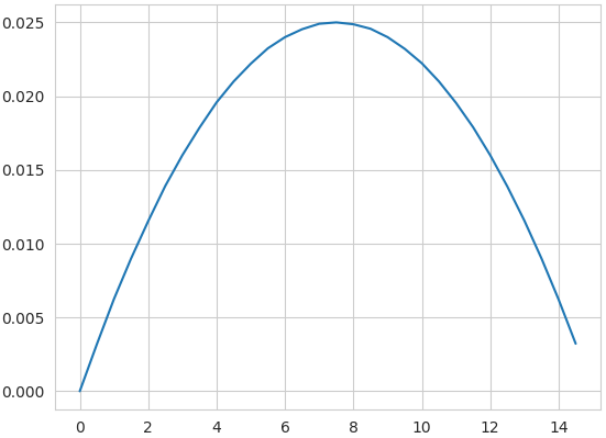
(a)	(b)

Figure 7: (a) Effective learning rate employed to train $noc$, in the P-NOC method. (b) Curve of mIoU measured over Pascal VOC 2012 training set, considering multiple choices of threshold $\delta_{\text{bg}}$.

Figure 7 (b) displays the sensitivity of mIoU to variations of the fg threshold. $P\textsuperscript{f}$ is only marginally better than the baseline (RA), while P-OC and P-NOC display higher area under the curve (mIoU) for almost all choices of the threshold, indicating that they are more robust and produce higher-quality segmentation priors with higher quality in for most choices.

Table 8: Scores (in IoU) measured over the Pascal VOC 2012 train set, per method. Class-specific properties, such as the average relative size (%S), class co-occurrence rate (%C) and average of label set cardinality (L) are listed for inspection purposes.

Class	Group	Size	%S	%C	L	RA	CSE	P	$\text{P}^{f}$	P-OC	P-NOC
bg	-	-	69.5%	-	-	81.0	82.2	85.6	86.0	85.6	86.8
a.plane	singleton	small	11.8%	9.1%	1.1	47.5	53.6	60.9	61.4	62.3	58.2
bicycle	traffic	small	6.4%	76.9%	2.2	32.2	34.7	41.2	38.6	45.0	42.8
bird	singleton	small	11.8%	11.4%	1.2	49.5	51.5	69.7	71.4	62.8	71.8
boat	p-rel	small	10.8%	32.1%	1.4	40.8	35.4	45.2	51.3	43.9	49.5
bottle	bottle	small	9.5%	70.1%	2.3	49.0	60.8	56.9	56.0	65.9	64.5
bus	traffic	large	31.5%	51.3%	1.7	72.1	65.9	79.6	78.4	75.1	80.6
car	traffic	mid	15.5%	61.7%	1.9	62.6	63.3	74.2	70.4	74.6	74.4
cat	animal	large	28.6%	26.0%	1.3	54.8	78.4	82.6	83.7	79.8	83.6
chair	room	small	10.6%	87.8%	2.4	30.7	24.0	28.9	27.2	23.1	28.9
cow	animal	mid	18.0%	29.7%	1.4	55.1	68.2	71.5	73.6	70.6	69.0
d.table	room	large	22.5%	95.1%	2.6	52.5	46.3	49.6	39.2	51.0	52.2
dog	animal	large	19.8%	38.0%	1.5	61.3	61.2	78.8	80.8	76.9	79.5
horse	animal	large	19.1%	47.1%	1.6	55.9	68.9	67.7	69.0	69.8	70.3
m.bike	traffic	large	19.6%	56.8%	1.7	67.8	68.3	74.4	73.2	76.6	75.9
person	person	mid	15.2%	83.0%	2.1	63.6	63.8	57.0	50.3	70.2	70.2
p.plant	room	small	11.2%	63.4%	2.1	46.8	42.5	57.8	56.3	57.2	56.1
sheep	singleton	large	19.7%	19.0%	1.3	55.3	75.0	75.0	75.9	73.9	73.6
sofa	room	large	21.6%	80.6%	2.4	50.0	45.3	40.9	35.5	34.8	43.6
train	singleton	large	26.6%	20.5%	1.2	63.9	45.5	68.9	68.2	50.9	68.0
tv.	room	mid	15.5%	65.1%	2.1	38.6	41.5	36.5	33.8	49.8	37.2
overall			19.8%	51.2%	1.8	53.9	56.0	62.0	61.0	61.9	63.7
small			10.3%	50.1%	1.8	42.4	43.2	51.5	51.7	51.5	53.1
mid			16.1%	59.9%	1.9	55.0	59.2	59.8	57.0	66.3	62.7
large			23.2%	48.3%	1.7	59.3	61.6	68.6	67.1	65.4	69.7
singleton				17.5%	15.0%	1.2	54.0	56.4	68.6	69.2	62.5	67.9
person			15.2%	83.0%	2.1	63.6	63.8	57.0	50.3	70.2	70.2
animal			21.4%	35.2%	1.4	56.8	69.2	75.1	76.8	74.3	75.6
room			16.3%	78.4%	2.3	43.7	39.9	42.7	38.4	43.2	43.6
traffic			18.3%	61.7%	1.9	58.7	58.0	67.3	65.1	67.8	68.4
$\rho$ %S			100.0	-18.0	-23.4	70.3	51.5	55.6	48.4	38.3	53.1
$\rho$ %C			-18.0	100.0	97.6	-22.9	-38.4	-60.6	-71.0	-42.9	-51.4
$\rho$ L			-23.4	97.6	100.0	-32.9	-44.5	-66.0	-75.8	-49.7	-58.2

Table 9: Intersection over Union (IoU %) of pseudo segmentation masks devised from P-NOC and refined with random walk, measured over MS COCO 2014 train and val subsets.

Class	Train	Val			Class	Train	Val
background	82.2	81.8			wine glass	40.0	42.7
person	56.0	55.1			cup	38.5	36.2
bicycle	55.6	55.3			fork	22.2	23.2
car	47.7	47.4			knife	26.2	27.8
motorcycle	71.0	70.3			spoon	15.3	17.3
airplane	60.8	56.3			bowl	17.6	16.6
bus	79.8	76.8			banana	64.4	62.9
train	67.2	68.4			apple	52.4	53.3
truck	58.3	54.6			sandwich	47.5	46.4
boat	48.3	49.0			orange	60.3	62.1
traffic light	43.2	46.6			broccoli	40.5	41.1
fire hydrant	76.4	77.4			carrot	27.7	28.4
stop sign	71.2	74.4			hot dog	58.6	55.1
parking meter	74.2	71.5			pizza	63.3	62.7
bench	40.2	40.4			donut	61.8	66.4
bird	65.9	62.3			cake	54.1	54.3
cat	76.8	76.5			chair	26.5	25.2
dog	77.9	76.1			couch	35.6	34.3
horse	68.2	68.1			potted plant	27.5	25.4
sheep	74.6	75.3			bed	47.8	44.5
cow	78.4	78.5			dining table	13.9	13.7
elephant	79.9	80.6			toilet	63.5	65.1
bear	83.7	85.0			tv	42.7	40.7
zebra	79.1	80.7			laptop	56.0	55.9
giraffe	72.1	73.6			mouse	28.1	23.2
backpack	27.0	28.0			remote	29.0	30.0
umbrella	63.8	63.3			keyboard	61.7	60.1
handbag	14.4	14.4			cell phone	60.9	65.5
tie	14.9	15.5			microwave	49.7	46.4
suitcase	53.2	54.1			oven	34.6	36.2
frisbee	43.6	50.4			toaster	34.0	36.5
skis	7.8	8.2			sink	37.6	34.4
snowboard	41.3	42.7			refrigerator	27.5	27.7
sports ball	51.8	54.5			book	40.3	37.9
kite	42.3	46.3			clock	26.2	25.3
baseball bat	24.7	19.1			vase	38.1	35.8
baseball glove	16.4	14.2			scissors	43.2	54.1
skateboard	28.0	26.5			teddy bear	72.0	71.8
surfboard	39.5	34.9			hair drier	42.3	29.1
tennis racket	18.6	20.0			toothbrush	37.5	37.3
bottle	40.6	40.0			avg. overall	47.9	47.7

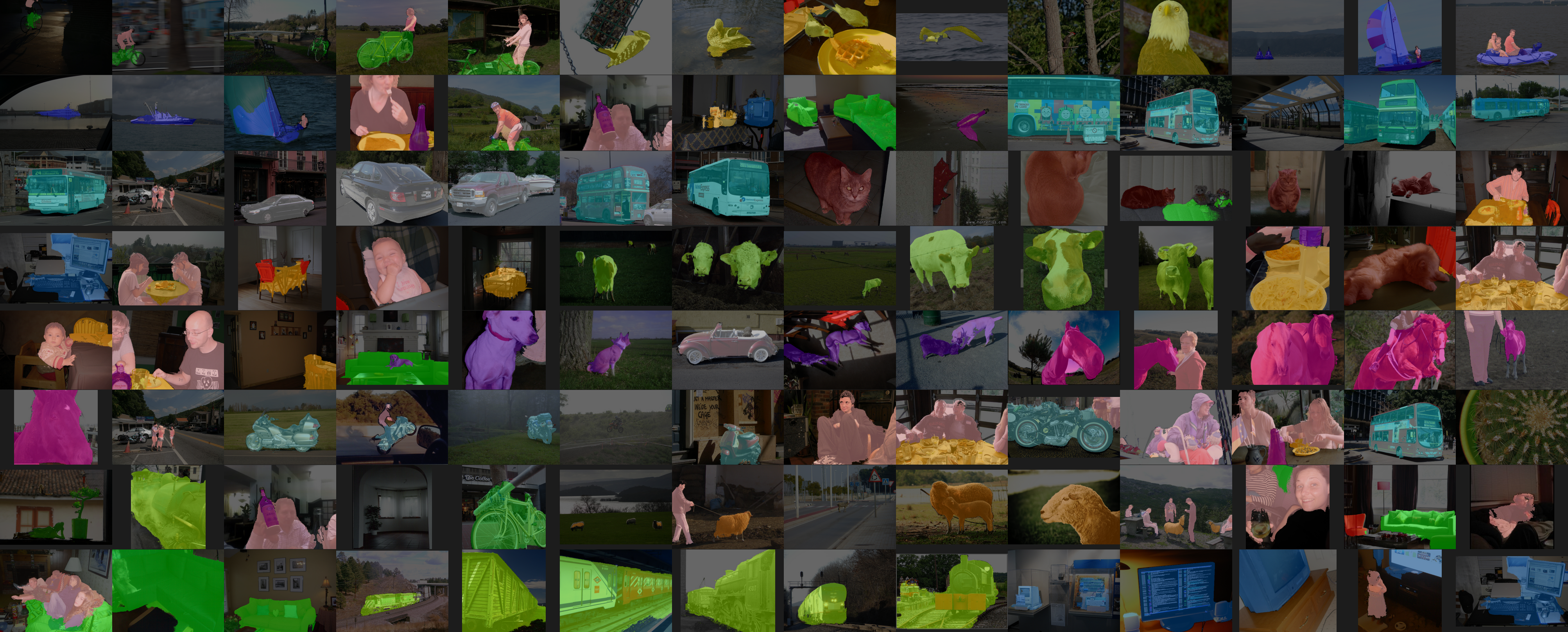
(a) P-OC+LS Pascal VOC 2012

(b) P-NOC+LS Pascal VOC 2012

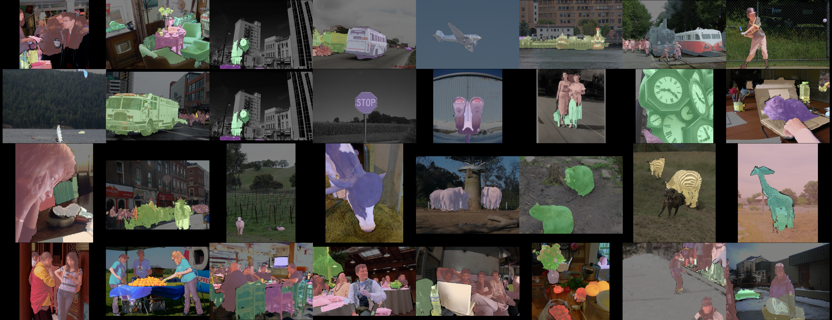
(c) P-NOC+ls MS COCO 2014

Figure 8: A and B: Segmentation examples for Pascal VOC 2012 by DeepLabV3+, trained over Pascal VOC 2012. Pseudo training masks were devised from (a) P-OC and (b) P-NOC+LS, respectively, and refined with C²AM-H, random walk and dCRF. B: P-NOC+LS. C: pseudo segmentation masks for MS COCO 2014, devised by P-NOC and refined with C²AM-H, random walk and dCRF.

References

- [1] Jiwoon Ahn, Sunghyun Cho, and Suha Kwak. Weakly supervised learning of instance segmentation with inter-pixel relations. In IEEE/CVF Conference on Computer Vision and Pattern Recognition (CVPR), pages 2209–2218, 2019.
- [2] Jiwoon Ahn and Suha Kwak. Learning pixel-level semantic affinity with image-level supervision for weakly supervised semantic segmentation. In IEEE/CVF Conference on Computer Vision and Pattern Recognition (CVPR), pages 4981–4990, 2018.
- [3] B. Bhanu and S. Lee. Genetic Learning for Adaptive Image Segmentation. The Springer International Series in Engineering and Computer Science. Springer US, 2012.
- [4] Arslan Chaudhry, Puneet K Dokania, and Philip HS Torr. Discovering class-specific pixels for weakly-supervised semantic segmentation. arXiv preprint arXiv:1707.05821, 2017.
- [5] Liang-Chieh Chen, Yukun Zhu, George Papandreou, Florian Schroff, and Hartwig Adam. Encoder-decoder with atrous separable convolution for semantic image segmentation. In European Conference on Computer Vision (ECCV), pages 801–818, 2018.
- [6] Yuantao Chen, Jiajun Tao, Linwu Liu, Jie Xiong, Runlong Xia, Jingbo Xie, Qian Zhang, and Kai Yang. Research of improving semantic image segmentation based on a feature fusion model. Journal of Ambient Intelligence and Humanized Computing, pages 1–13, 2020.
- [7] Ekin D Cubuk, Barret Zoph, Jonathon Shlens, and Quoc V Le. Randaugment: Practical automated data augmentation with a reduced search space. In IEEE/CVF Conference on Computer Vision and Pattern Recognition Workshops (CVPRW), pages 702–703, 2020.
- [8] Mark Everingham, SM Ali Eslami, Luc Van Gool, Christopher KI Williams, John Winn, and Andrew Zisserman. The PASCAL Visual Object Classes Challenge: A retrospective. International Journal of Computer Vision, 111(1):98–136, 2015.
- [9] Junsong Fan, Zhaoxiang Zhang, Chunfeng Song, and Tieniu Tan. Learning integral objects with intra-class discriminator for weakly-supervised semantic segmentation. In IEEE/CVF Conference on Computer Vision and Pattern Recognition (CVPR), pages 4283–4292, 2020.
- [10] Fraol Gelana and Arvind Yadav. Firearm detection from surveillance cameras using image processing and machine learning techniques. In Smart Innovations in Communication and Computational Sciences, pages 25–34. Springer, 2019.
- [11] Peng-Tao Jiang, Yuqi Yang, Qibin Hou, and Yunchao Wei. L2g: A simple local-to-global knowledge transfer framework for weakly supervised semantic segmentation. In IEEE/CVF Conference on Computer Vision and Pattern Recognition (CVPR), pages 16886–16896, 2022.
- [12] Sanghyun Jo and In-Jae Yu. Puzzle-cam: Improved localization via matching partial and full features. In IEEE International Conference on Image Processing (ICIP), pages 639–643, 2021.
- [13] Philipp Krähenbühl and Vladlen Koltun. Efficient inference in fully connected CRFs with gaussian edge potentials. Advances in Neural Information Processing Systems (NeurIPS), 24:109–117, 2011.
- [14] Viveka Kulharia, Siddhartha Chandra, Amit Agrawal, Philip Torr, and Ambrish Tyagi. Box2seg: Attention weighted loss and discriminative feature learning for weakly supervised segmentation. In European Conference on Computer Vision (ECCV), pages 290–308. Springer, 2020.
- [15] Hyeokjun Kweon, Sung-Hoon Yoon, Hyeonseong Kim, Daehee Park, and Kuk-Jin Yoon. Unlocking the potential of ordinary classifier: Class-specific adversarial erasing framework for weakly supervised semantic segmentation. In IEEE/CVF International Conference on Computer Vision (ICCV), pages 6974–6983, 2021.
- [16] Rodney LaLonde, Ziyue Xu, Ismail Irmakci, Sanjay Jain, and Ulas Bagci. Capsules for biomedical image segmentation. Medical Image Analysis, 68:101889, 2021.
- [17] Jungbeom Lee, Jooyoung Choi, Jisoo Mok, and Sungroh Yoon. Reducing information bottleneck for weakly supervised semantic segmentation. Advances in Neural Information Processing Systems (NeurIPS), 34:27408–27421, 2021.
- [18] Jungbeom Lee, Jooyoung Choi, Jisoo Mok, and Sungroh Yoon. Reducing information bottleneck for weakly supervised semantic segmentation. Advances in Neural Information Processing Systems, 34:27408–27421, 2021.
- [19] Jungbeom Lee, Jihun Yi, Chaehun Shin, and Sungroh Yoon. BBAM: Bounding box attribution map for weakly supervised semantic and instance segmentation. In IEEE/CVF Conference on Computer Vision and Pattern Recognition (CVPR), pages 2643–2652, 2021.
- [20] Minhyun Lee, Dongseob Kim, and Hyunjung Shim. Threshold matters in wsss: Manipulating the activation for the robust and accurate segmentation model against thresholds. In IEEE/CVF Conference on Computer Vision and Pattern Recognition (CVPR), pages 4330–4339, 2022.
- [21] Seungho Lee, Minhyun Lee, Jongwuk Lee, and Hyunjung Shim. Railroad is not a train: Saliency as pseudo-pixel supervision for weakly supervised semantic segmentation. In IEEE/CVF Conference on Computer Vision and Pattern Recognition (CVPR), pages 5495–5505, 2021.
- [22] Kunpeng Li, Ziyan Wu, Kuan-Chuan Peng, Jan Ernst, and Yun Fu. Tell me where to look: Guided attention inference network. In IEEE/CVF Conference on Computer Vision and Pattern Recognition (CVPR), pages 9215–9223, 2018.
- [23] Yi Li, Yiqun Duan, Zhanghui Kuang, Yimin Chen, Wayne Zhang, and Xiaomeng Li. Uncertainty estimation via response scaling for pseudo-mask noise mitigation in weakly-supervised semantic segmentation. In AAAI Conference on Artificial Intelligence, volume 36, pages 1447–1455, 2022.
- [24] Yi Li, Zhanghui Kuang, Liyang Liu, Yimin Chen, and Wayne Zhang. Pseudo-mask matters in weakly-supervised semantic segmentation. In IEEE/CVF International Conference on Computer Vision (CVPR), pages 6964–6973, 2021.
- [25] Tsung-Yi Lin, Michael Maire, Serge Belongie, James Hays, Pietro Perona, Deva Ramanan, Piotr Dollár, and C Lawrence Zitnick. Microsoft COCO: Common objects in context. In European Conference on Computer Vision (ECVV), pages 740–755. Springer, 2014.
- [26] Xiaofeng Liu, Yuzhuo Han, Song Bai, Yi Ge, Tianxing Wang, Xu Han, Site Li, Jane You, and Jun Lu. Importance-aware semantic segmentation in self-driving with discrete wasserstein training. In AAAI Conference on Artificial Intelligence, volume 34, pages 11629–11636, 2020.
- [27] Yujian Mo, Yan Wu, Xinneng Yang, Feilin Liu, and Yujun Liao. Review the state-of-the-art technologies of semantic segmentation based on deep learning. Neurocomputing, 493:626–646, 2022.
- [28] Rafael Müller, Simon Kornblith, and Geoffrey E Hinton. When does label smoothing help? Advances in Neural Information Processing Systems (NIPS), 32, 2019.
- [29] Seong Joon Oh, Rodrigo Benenson, Anna Khoreva, Zeynep Akata, Mario Fritz, and Bernt Schiele. Exploiting saliency for object segmentation from image level labels. In IEEE/CVF Conference on Computer Vision and Pattern Recognition (CVPR), pages 5038–5047, 2017.
- [30] Youngmin Oh, Beomjun Kim, and Bumsub Ham. Background-aware pooling and noise-aware loss for weakly-supervised semantic segmentation. In IEEE/CVF Conference on Computer Vision and Pattern Recognition (CVPR), pages 6913–6922, 2021.
- [31] Youssef Ouassit, Soufiane Ardchir, Mohammed Yassine El Ghoumari, and Mohamed Azouazi. A brief survey on weakly supervised semantic segmentation. International Journal of Online & Biomedical Engineering, 18(10), 2022.
- [32] Simone Rossetti, Damiano Zappia, Marta Sanzari, Marco Schaerf, and Fiora Pirri. Max pooling with vision transformers reconciles class and shape in weakly supervised semantic segmentation. In European Conference on Computer Vision (ECCV), pages 446–463. Springer, 2022.
- [33] Fengdong Sun and Wenhui Li. Saliency guided deep network for weakly-supervised image segmentation. Pattern Recognition Letters, 120:62–68, 2019.
- [34] Christian Szegedy, Vincent Vanhoucke, Sergey Ioffe, Jon Shlens, and Zbigniew Wojna. Rethinking the inception architecture for computer vision. In IEEE/CVF Conference on Computer Vision and Pattern Recognition (CVPR), pages 2818–2826, 2016.
- [35] Giulia Vilone and Luca Longo. Explainable artificial intelligence: a systematic review. arXiv preprint arXiv:2006.00093, 2020.
- [36] Yuchao Wang, Haochen Wang, Yujun Shen, Jingjing Fei, Wei Li, Guoqiang Jin, Liwei Wu, Rui Zhao, and Xinyi Le. Semi-supervised semantic segmentation using unreliable pseudo-labels. In IEEE/CVF Conference on Computer Vision and Pattern Recognition (CVPR), pages 4238–4247, 2022.
- [37] Yude Wang, Jie Zhang, Meina Kan, Shiguang Shan, and Xilin Chen. Self-supervised equivariant attention mechanism for weakly supervised semantic segmentation. In IEEE/CVF Conference on Computer Vision and Pattern Recognition (CVPR), pages 12275–12284, 2020.
- [38] Jinheng Xie, Jianfeng Xiang, Junliang Chen, Xianxu Hou, Xiaodong Zhao, and Linlin Shen. C²AM: Contrastive learning of class-agnostic activation map for weakly supervised object localization and semantic segmentation. In IEEE/CVF Conference on Computer Vision and Pattern Recognition (CVPR), pages 989–998, 2022.
- [39] Lian Xu, Wanli Ouyang, Mohammed Bennamoun, Farid Boussaid, and Dan Xu. Multi-class token transformer for weakly supervised semantic segmentation. In IEEE/CVF Conference on Computer Vision and Pattern Recognition (CVPR), pages 4300–4309, 2022.
- [40] Zongqian Zhan, Xiaomeng Zhang, Yi Liu, Xiao Sun, Chao Pang, and Chenbo Zhao. Vegetation land use/land cover extraction from high-resolution satellite images based on adaptive context inference. IEEE Access, 8:21036–21051, 2020.
- [41] Bingfeng Zhang, Jimin Xiao, Yunchao Wei, Kaizhu Huang, Shan Luo, and Yao Zhao. End-to-end weakly supervised semantic segmentation with reliable region mining. Pattern Recognition, 128:108663, 2022.
- [42] Dong Zhang, Hanwang Zhang, Jinhui Tang, Xian-Sheng Hua, and Qianru Sun. Causal intervention for weakly-supervised semantic segmentation. Advances in Neural Information Processing Systems, 33:655–666, 2020.
- [43] Bolei Zhou, Aditya Khosla, Agata Lapedriza, Aude Oliva, and Antonio Torralba. Learning deep features for discriminative localization. In IEEE/CVF Conference on Computer Vision and Pattern Recognition (CVPR), June 2016.