Polarization modes of gravitational waves in generalized Proca theory

Abstract

Abstract: In this paper, we study polarization modes of gravitational waves in generalized Proca theory in the homogeneous and isotropic Minkowski background. The results show that the polarizations of gravitational waves depend on the parameter space of this gravity theory and can be divided into quite rich cases by parameters. In some parameter space, it only allows two tensor modes, i.e., the $+$ and $\times$ modes. In some parameter space, besides tensor modes, it also allows one scalar mode, or two vector (vector-$x$ and vector-$y$) modes, or both one scalar mode and two vector modes. The scalar mode is a mixture mode of a breathing mode and a longitudinal mode, or just a pure breathing mode. Interestingly, it is found that the amplitude of the vector modes is related to the speed of the tensor modes. This allows us to give the upper bound of the amplitude of the vector modes by detecting the speed of the tensor modes. Specifically, if the speed of tensor modes is strictly equal to the speed of light, then the amplitude of vector modes is zero.

I Introduction

The successful detection of gravitational waves Abbott1 ; Abbott2 ; Abbott3 ; Abbott4 ; Abbott5 implies the arrival of the gravitational wave astronomy era. In addition to using electromagnetic waves, we can also develop astronomy and cosmology by detecting gravitational waves Shi Pi ; Andrea Addazi ; Rong-Gen Cai ; Zhi-Chao Zhao ; Zong-Kuan Guo . Not only that, gravitational waves can also help us test various modified gravities and deepen our understanding of gravity R. Cai2 ; Ligong Bian .

Polarization is an important property of gravitational waves. In four-dimensional space-time, there are at most six independent polarization modes of gravitational waves Eardley . For a specific modified gravity, due to the constraints of the field equations, it generally does not allow all six polarization modes, but rather allows a subset of them. Different theories predict different classes of polarization modes, so it can be expected that some of them will be excluded from the detection of polarization modes of gravitational waves in the future.

In many modified gravities, the polarization modes of gravitational waves have been studied , like $f(R)$, Horndeski, Palatini generalized Brans-Dicke, Palatini Horndeski, teleparallel Horndeski, Einstein-ather, tensor-vector-scalar, Horava, scalar-tensor-vector, $f(T)$, dCS, EdGB and Bumblebee theories f(R ; Horndeski0 ; TeVeS ; Horava ; STVG ; fT ; dCS and EdGB ; Y.Dong ; L.Shao ; S. Bahamonde ; J.Lu . The ground-based gravitational wave detectors of LIGO, VIRGO and KAGRA are located at different locations on the Earth. They can detect gravitational waves in different two-dimensional planes. Therefore, different detectors can cooperate to detect the polarization modes of gravitational waves. In this regard, some related work has already begun Abbott4 ; Abbott5 ; H. Takeda ; B. P . Abbottet al.1 ; B. P . Abbottet al.2 ; B. P . Abbottet al.3 ; Atsushi Nishizawa ; Kazuhiro Hayama ; Maximiliano Isi1 ; Maximiliano Isi2 ; K. Chatziioannou ; Hiroki Takeda ; Yuki Hagihara ; Peter T. H. Pang ; B. P . Abbottet al.4 . Polarization information of gravitational waves can also be detected using Pulsar Timing Arrays (PTA) YiPeng Jing . For example, in 2021, Huang et al. discovered a tentative indication for scalar transverse gravitational waves in NANOGrav 12.5-year data set Z. Chen . Furthermore, one can also expect to use space gravitational wave detectors such as Lisa, Taiji and TianQin lisa ; taiji ; Lisa-taiji ; tianqin to detect polarization modes of gravitational waves in the future.

Adding additional field is one way to modify gravity. The additional degrees of freedom may explain inflation and the accelerated expansion of the Universe AA.Starobinsky ; A. H. Guth ; K.Sato ; L.Heisenberg0 . If the additional field is a scalar field, then such a theory is called scalar-tensor theory. In the metric formalism, the most general scalar-tensor theory that can derive second-order field equations is Horndeski theory Horndeski . This theory was first discovered by Horndeski in 1974. Later, one realized that extending the scalar Galileon theory A. Nicolis to curved space-time would lead to the rediscovery of Horndeski theory C. Deffayet1 ; C. Deffayet2 .

In addition to adding a scalar field, we can also add an additional vector field to modify gravity. Such a theory is called vector-tensor theory. Similar to the scalar Galileon theory, in 2014, Heisenberg constructed a vector Galileon theory and extended it to the case of curved space-time Heisenberg . This covariant vector-tensor theory constitutes the Galileon-type generalization of the Proca action, and it is called generalized Proca theory. Generalized Proca theory is extended to vector Galileon theory. The corresponding field equations are second-order, so there is no the Ostrogradsky instability in this generalized Proca theory M.Ostrogradsky . There has been a lot of research on this theory, such as cosmology Antonio De Felice ; Lavinia Heisenberg ; Chao Qiang Geng and black holes Eugeny Babichev ; Lavinia Heisenberg2 ; Lavinia Heisenberg3 ; Sebastian Garcia-Saenz .

In this paper, we will study polarization modes of gravitational waves in generalized Proca theory in the range of a linear analysis. We consider a homogeneous and isotropic Minkowski background and our goal is to obtain the linearized field equations and then analyze the polarization modes of gravitational waves allowed by these equations. Therefore, in Sec. II, we review the action of generalized Proca theory. In Sec. III, we obtain the background equations and linear perturbation equations. In Sec. IV, we combine the perturbations into some gauge invariants. These gauge invariants can help us analyze the linear perturbation equations. In Sec. V, we analyze the polarization modes of gravitational waves in generalized Proca theory.

We will use the natural system of units $c=G=1$ and consider four-dimensional space-time in this paper. We set the metric signature as $(-,+,+,+)$. The Latin alphabet indices $(a,b,c,d,e)$ range over space-time indices ($0,1,2,3$), and the Latin alphabet indices $(i,j,k)$ range over space indices ($1,2,3$) which point to ($+x,+y,+z$) directions respectively.

II generalized Proca theory

Generalized Proca theory is a vector-tensor theory. In addition to being related to the metric $g_{ab}$, the action also depends on a vector field $A^{a}$.

The action of generalized Proca theory is Heisenberg ; Antonio De Felice ; Antonio De Felice2

$$S\left(g_{ab},A^{a}\right)=\int d^{4}x\sqrt{-g}~{}\Bigl{(}\mathcal{L}_{F}+\mathcal{L}_{2}+\mathcal{L}_{3}+\mathcal{L}_{4}+\mathcal{L}_{5}\Bigl{)},$$ (1)

where

$$\mathcal{L}_{F} = -\frac{1}{4}F_{ab}F^{ab},$$ (2)

$$\mathcal{L}_{2} = G_{2}(X),$$ (3)

$$\mathcal{L}_{3} = G_{3}(X)\nabla_{a}A^{a},$$ (4)

$$\mathcal{L}_{4} = G_{4}(X){R}+G_{4,X}(X)\left[\left(\nabla_{a}A^{a}\right)^{2}+c_{2}\nabla_{a}A_{b}\nabla^{a}A^{b}-\left(1+c_{2}\right)\nabla_{a}A_{b}\nabla^{b}A^{a}\right],$$ (5)

$$\mathcal{L}_{5} = G_{5}(X)\left({R}_{ab}-\frac{1}{2}{g}_{ab}{R}\right)\nabla^{a}A^{b}$$ (6)

$$- \frac{1}{6}G_{5,X}(X)\left[\left(\nabla_{a}A^{a}\right)^{3}-3d_{2}\nabla_{a}A^{a}\nabla_{b}A_{c}\nabla^{b}A^{c}-3\left(1-d_{2}\right)\nabla_{a}A^{a}\nabla_{b}A_{c}\nabla^{c}A^{b}\right.$$

$$+ \left.\left(2-3d_{2}\right)\nabla_{a}A_{b}\nabla^{c}A^{a}\nabla^{b}A_{c}+3d_{2}\nabla_{a}A_{b}\nabla^{c}A^{a}\nabla_{c}A^{b}\right].$$

Here, $F_{ab}=\nabla_{a}A_{b}-\nabla_{b}A_{a}$, $R_{ab}$ is the Ricci tensor and $R$ is the Ricci scalar, $c_{2},d_{2}$ are constants, $G_{2},G_{3},G_{4}$ and $G_{5}$ are arbitrary functions of the variable $X=-\frac{1}{2}g_{ab}A^{a}A^{b}$. In addition, $G_{n,X}={dG_{n}}/{dX}$ ($n=2,3,4,5$). The remaining derivatives are still represented by this notation. For example, $G_{2,{XX}}$ represents the second-order derivative of $G_{2}$ with respect to the variable $X$.

The first term of $\mathcal{L}_{4}$ can be equivalently written as $(16\pi)^{-1}R+\left[G_{4}(X)-(16\pi)^{-1}\right]R$. Therefore, it is easy to see that this theory includes the Einstein-Hilbert action. We hope that generalized Proca theory can retain the contribution of the Einstein-Hilbert term, so it requires

$$G_{4}(X)\neq 0.$$ (7)

III Background equations and linear perturbation equations

Now consider a homogeneous and isotropic Minkowski background

$$g_{ab}=\eta_{ab},\quad A^{a}=\mathring{A}^{a}=\left(A,0,0,0\right),$$ (8)

where $\mathring{A}^{a}$ is a constant vector and $\eta_{ab}$ is the Minkowski metric. Due to spatial isotropy, the vector $\mathring{A}^{a}$ only has one nonvanishing temporal component $A$, and its spatial components are all zero.

By substituting the assumption (8) into the field equations derived from the variation of the action (1), we can know that $\mathring{A}^{a}$ should satisfy the following background equations:

$$-\frac{1}{2}\mathring{G}_{2}\eta_{ab}+\frac{1}{2}\mathring{G}_{2,X}\mathring{A}_{a}\mathring{A}_{b} = 0,$$ (9)

$$-\mathring{G}_{2,X}\mathring{A}_{a} = 0.$$ (10)

Here and below, the notation “$\circ$” above the letter means that the corresponding function takes the value of $X=-\frac{1}{2}\eta_{ab}\mathring{A}^{a}\mathring{A}^{b}$. Using the background equations (9) and (10), we can divide the background solution (8) into two cases:

Case A: $\mathring{G}_{2}=0,~{}\mathring{G}_{2,X}\neq 0,~{}A=0$.

Case B: $\mathring{G}_{2}=0,~{}\mathring{G}_{2,X}=0$, $A=\text{constant}$.

To describe gravitational waves, we investigate perturbations of the background

$$g_{ab}=\eta_{ab}+h_{ab},\quad A^{a}=\mathring{A}^{a}+B^{a}.$$ (11)

In the following, we use $\eta_{ab}$ and $\eta^{ab}$ to lower and raise the space-time index and define $h=\eta^{ab}h_{ab}$.

By substituting the perturbations (11) into the field equations derived from the variation of the action (1), and writing the first-order terms of the perturbations, we can obtain two linear perturbation equations that describes gravitational waves.

Substituting the perturbations into the field equation derived from the variation of vector $A^{a}$, we obtain the first linear perturbation equation

$$2\Box B_{a}-2\mathring{A}^{b}\partial_{a}\partial_{c}h^{c}_{~{}b}+2\mathring{A}^{b}\Box h_{ab}-2\mathring{G}_{2,X}B_{a}-2\mathring{G}_{2,X}\mathring{A}^{b}h_{ab}$$ (12)

$$+ 2\mathring{G}_{3,X}\mathring{A}^{b}\partial_{a}B_{b}+\mathring{G}_{3,X}\mathring{A}^{b}\mathring{A}^{c}\partial_{a}h_{bc}-2\mathring{G}_{3,X}\mathring{A}_{a}\partial_{b}B^{b}-\mathring{G}_{3,X}\mathring{A}_{a}\mathring{A}^{b}\partial_{b}h$$

$$- 4\mathring{G}_{4,X}\partial_{a}\partial_{b}B^{b}-2\mathring{G}_{4,X}\mathring{A}^{b}\partial_{a}\partial_{b}h-4c_{2}\mathring{G}_{4,X}\Box B_{a}+2\mathring{G}_{4,X}\mathring{A}^{b}\partial_{a}\partial_{c}h_{b}^{~{}c}$$

$$+ 4c_{2}\mathring{G}_{4,X}\mathring{A}^{b}\partial_{a}\partial_{c}h_{b}^{~{}c}+2\mathring{G}_{4,X}\mathring{A}^{b}\partial_{b}\partial_{c}h_{a}^{~{}c}-2\mathring{G}_{4,X}\mathring{A}_{a}\partial_{b}\partial_{c}h^{bc}-2\mathring{G}_{4,X}\mathring{A}^{b}\Box h_{ab}$$

$$- 4c_{2}\mathring{G}_{4,X}\mathring{A}^{b}\Box h_{ab}+2\mathring{G}_{4,X}\mathring{A}_{a}\Box h+\left[-2+4\left(1+c_{2}\right)\mathring{G}_{4,X}\right]\partial_{a}\partial_{b}B^{b}$$

$$+ 2\mathring{G}_{2,XX}\mathring{A}_{a}\mathring{A}^{b}B_{b}+\mathring{G}_{2,XX}\mathring{A}_{a}\mathring{A}^{b}\mathring{A}^{c}h_{bc}~{}=~{}0.$$

Substituting the perturbations into the field equation derived from the variation of tensor $g^{ab}$, we have the second linear perturbation equation

$$- 2\mathring{G}_{2}h_{ab}-2\mathring{A}_{b}\Box B_{a}-2\mathring{A}_{a}\Box B_{b}+2\mathring{A}_{b}\partial_{a}\partial_{c}B^{c}+2\mathring{A}_{a}\partial_{b}\partial_{c}B^{c}$$ (13)

$$+ 2\mathring{A}_{b}\mathring{A}^{c}\partial_{a}\partial_{d}h_{c}^{~{}d}+2\mathring{A}_{a}\mathring{A}^{c}\partial_{b}\partial_{d}h_{c}^{~{}d}-2\mathring{A}_{b}\mathring{A}^{c}\Box h_{ac}-2\mathring{A}_{a}\mathring{A}^{c}\Box h_{bc}$$

$$- 2\mathring{G}_{4}\left(\partial_{a}\partial_{b}h-\partial_{a}\partial_{c}h^{c}_{~{}b}-\partial_{b}\partial_{c}h^{c}_{~{}a}+\Box h_{ab}+\eta_{ab}\partial_{c}\partial_{d}h^{cd}-\eta_{ab}\Box h\right)$$

$$+ 2\mathring{G}_{2,X}\mathring{A}_{b}B_{a}+2\mathring{G}_{2,X}\mathring{A}_{a}B_{b}+2\mathring{G}_{2,X}\eta_{ab}\mathring{A}^{c}B_{c}+2\mathring{G}_{2,X}\mathring{A}_{b}\mathring{A}^{c}h_{ac}$$

$$+ 2\mathring{G}_{2,X}\mathring{A}_{a}\mathring{A}^{c}h_{bc}+\mathring{G}_{2,X}\eta_{ab}\mathring{A}^{c}\mathring{A}^{d}h_{cd}+2\mathring{G}_{3,X}\mathring{A}_{a}\mathring{A}_{b}\partial_{c}B^{c}$$

$$+ \mathring{G}_{3,X}\mathring{A}_{a}\mathring{A}_{b}\mathring{A}^{c}\partial_{c}h-2\mathring{G}_{3,X}\eta_{ab}\mathring{A}^{c}\mathring{A}^{d}\partial_{d}B_{c}-\mathring{G}_{3,X}\eta_{ab}\mathring{A}^{c}\mathring{A}^{d}\mathring{A}^{e}\partial_{e}h_{cd}$$

$$+ 2\mathring{G}_{4,X}\mathring{A}^{c}\partial_{a}\partial_{b}B_{c}+\mathring{G}_{4,X}\mathring{A}^{c}\mathring{A}^{d}\partial_{a}\partial_{b}h_{cd}+2\mathring{G}_{4,X}\mathring{A}^{c}\partial_{a}\partial_{b}B_{c}$$

$$+ \mathring{G}_{4,X}\mathring{A}^{c}\mathring{A}^{d}\partial_{a}\partial_{b}h_{cd}-2\mathring{G}_{4,X}\mathring{A}^{c}\partial_{c}\partial_{a}B_{b}-2\mathring{G}_{4,X}\mathring{A}_{b}\partial_{a}\partial_{c}B^{c}$$

$$- 4c_{2}\mathring{G}_{4,X}\mathring{A}_{b}\partial_{a}\partial_{c}B^{c}-2\mathring{G}_{4,X}\mathring{A}^{c}\partial_{c}\partial_{b}B_{a}-2\mathring{G}_{4,X}\mathring{A}_{a}\partial_{b}\partial_{c}B^{c}$$

$$- 4c_{2}\mathring{G}_{4,X}\mathring{A}_{a}\partial_{b}\partial_{c}B^{c}+2\mathring{G}_{4,X}\mathring{A}_{b}\Box B_{a}+4c_{2}\mathring{G}_{4,X}\mathring{A}_{b}\Box B_{a}$$

$$+ 2\mathring{G}_{4,X}\mathring{A}_{a}\Box B_{b}+4c_{2}\mathring{G}_{4,X}\mathring{A}_{a}\Box B_{b}+4\mathring{G}_{4,X}\eta_{ab}\mathring{A}^{c}\partial_{c}\partial_{d}B^{d}$$

$$- 2\mathring{G}_{4,X}\mathring{A}_{b}\mathring{A}^{c}\partial_{a}\partial_{d}h_{c}^{~{}d}-4c_{2}\mathring{G}_{4,X}\mathring{A}_{b}\mathring{A}^{c}\partial_{a}\partial_{d}h_{c}^{~{}d}-2\mathring{G}_{4,X}\mathring{A}_{a}\mathring{A}^{c}\partial_{b}\partial_{d}h_{c}^{~{}d}$$

$$- 4c_{2}\mathring{G}_{4,X}\mathring{A}_{a}\mathring{A}^{c}\partial_{b}\partial_{d}h_{c}^{~{}d}-2\mathring{G}_{4,X}\mathring{A}^{c}\mathring{A}^{d}\partial_{c}\partial_{d}h_{ab}+2\mathring{G}_{4,X}\mathring{A}_{a}\mathring{A}_{b}\partial_{c}\partial_{d}h^{cd}$$

$$+ 2\mathring{G}_{4,X}\eta_{ab}\mathring{A}^{c}\mathring{A}^{d}\partial_{c}\partial_{d}h-4G_{4,X}\eta_{ab}\mathring{A}^{c}\Box B_{c}+2\mathring{G}_{4,X}\mathring{A}_{b}\mathring{A}^{c}\Box h_{ac}$$

$$+ 4c_{2}\mathring{G}_{4,X}\mathring{A}_{b}\mathring{A}^{c}\Box h_{ac}+2\mathring{G}_{4,X}\mathring{A}_{a}\mathring{A}^{c}\Box h_{bc}+4c_{2}\mathring{G}_{4,X}\mathring{A}_{a}\mathring{A}^{c}\Box h_{bc}$$

$$- 2\mathring{G}_{4,X}\mathring{A}_{a}\mathring{A}_{b}\Box h-2\mathring{G}_{4,X}\eta_{ab}\mathring{A}^{c}\mathring{A}^{d}\Box h_{cd}-2\mathring{G}_{2,XX}\mathring{A}_{a}\mathring{A}_{b}\mathring{A}^{c}B_{c}$$

$$- \mathring{G}_{2,XX}\mathring{A}_{a}\mathring{A}_{b}\mathring{A}^{c}\mathring{A}^{d}h_{cd}~{}=~{}0.$$

It should be noted that for the case of $A=0$, i.e., $\mathring{A}^{a}=0$, it is easy to analyze polarization modes of gravitational waves. In this case, Eq. (13) becomes

$$-2\mathring{G}_{2}h_{ab}-2\mathring{G}_{4}\left(\partial_{a}\partial_{b}h-\partial_{a}\partial_{c}h^{c}_{~{}b}-\partial_{b}\partial_{c}h^{c}_{~{}a}+\Box h_{ab}+\eta_{ab}\partial_{c}\partial_{d}h^{cd}-\eta_{ab}\Box h\right)=0.$$ (14)

On the other hand, we always have $\mathring{G}_{2}=0$ for the background solution (8). In addition, since $G_{4}(X)\neq 0$, Eq. (14) can be further written as

$$\mathop{G}^{(1)}~\!\!\!{}_{ab}=-\frac{1}{2}\left(\partial_{a}\partial_{b}h-\partial_{a}\partial_{c}h^{c}_{~{}b}-\partial_{b}\partial_{c}h^{c}_{~{}a}+\Box h_{ab}+\eta_{ab}\partial_{c}\partial_{d}h^{cd}-\eta_{ab}\Box h\right)=0.$$ (15)

Here, $G_{ab}$ is the Einstein tensor, and the notation “$(1)$” above the letter $G$ means that only the first-order term of the perturbations is taken here. It can be seen that under linear approximation, Eq. (15) is no different from Einstein’s field equation. Therefore, just like general relativity, there are only two tensor modes ($+$ and $\times$) propagating at the speed of light for the case of $A=0$.

One may ask whether another linear perturbation equation (12) further constrains the tensor mode gravitational waves. The answer is no. Note that only the transverse traceless part $h^{TT}_{ij}$ of the metric perturbation $h_{ab}$ contributes to the tensor mode gravitational waves, and Eq. (12) is a vector type equation with a single index. We can know that this equation does not constrain the value of $h^{TT}_{ij}$, and therefore does not constrain the tensor mode gravitational waves.

Through the above analysis, we find that when the background solution (8) belongs to Case A, it only allows two tensor ($+$ and $\times$) modes propagating at the speed of light. The result is the same for Case B with $A=0$. Therefore, in the following sections, we only need to analyze the case where the background solution (8) meets the following conditions:

$$\mathring{G}_{2}=0,~{}\mathring{G}_{2,X}=0,~{}A\neq 0.$$ (16)

IV gauge invariants

In this section, we will introduce a method for simplifying linear perturbation equations. After using this method, the linear perturbation equations can be decomposed into independent tensor, vector, and scalar equations. These equations can be represented by some gauge invariants combined with perturbations.

Under spatial rotation transformation, $h_{ij}$ is transformed like a second-order tensor, $h_{0i}$, $B^{i}$ are transformed like vectors, and $h_{00}$, $B^{0}$ are transformed like scalars. We can uniquely decompose the perturbations as follows R. Jackiw ; Eanna E Flanagan ; L.Shao :

$$B^{0} = B^{0},$$

$$B^{i} = \partial^{i}\omega+\mu^{i},$$

$$h_{00} = h_{00},$$ (17)

$$h_{0i} = \partial_{i}\gamma+\beta_{i},$$

$$h_{ij} = h^{TT}_{ij}+\partial_{i}\epsilon_{j}+\partial_{j}\epsilon_{i}+\frac{1}{3}\delta_{ij}H+(\partial_{i}\partial_{j}-\frac{1}{3}\delta_{ij}\Delta)\zeta.$$

Here,

$$\partial_{i}\mu^{i}=\partial_{i}\beta^{i}=\partial_{i}\epsilon^{i}=0,$$ (18)

$$\delta^{ij}h^{TT}_{ij}=\partial^{i}h^{TT}_{ij}=0.$$ (19)

Here and below, we use $\delta_{ij}$ and $\delta^{ij}$ to lower and raise the space index. As can be seen, Eq. (IV) uniquely decomposes a spatial vector into a scalar part and a transverse vector part, and uniquely decomposes a spatial tensor into two scalar parts, a transverse vector part, and a transverse traceless tensor part.

Considering that the left sides of Eqs. (12) and (13) are actually a vector and a tensor, respectively, we can also apply this decomposition method to the linear perturbation equations. Due to the uniqueness of the decomposition, requiring the equations to be zero is equivalent to requiring that each decomposed part of the linear perturbation equations be zero, so we can obtain a series of independent tensor, vector and scalar equations. Due to the spatial homogeneous and isotropic of the background solution (8), by substituting (IV) into Eqs. (12) and (13), we can see that these decomposed scalar, vector and tensor equations only rely on tensor, vector and scalar perturbations, respectively Weinberg . Therefore, the linear perturbation equations are decoupled.

We can also continue to combine the perturbations in these equations into gauge invariants.

Under linear approximation, the gauge transformations of the metric and the vector field are Robert Bluhm

$$h_{ab} \rightarrow h_{ab}-\partial_{a}\xi_{b}-\partial_{b}\xi_{a},$$ (20)

$$B^{a} \rightarrow B^{a}+\mathring{A}^{b}\partial_{b}\xi^{a}.$$ (21)

Here, $\xi^{a}$ is an arbitrary function of space-time coordinates.

Under the above gauge transformations, the spatial tensor

$$h^{TT}_{ij},$$ (22)

the two spatial vectors

$$\begin{array}[]{l}\Xi_{i}=\beta_{i}-\partial_{0}\epsilon_{i},\\ \Sigma_{i}=\mu_{i}+A\partial_{0}\epsilon_{i},\end{array}$$ (25)

and the four spatial scalars

$$\begin{array}[]{l}\phi\,=-\frac{1}{2}h_{00}+\partial_{0}\gamma-\frac{1}{2}\partial_{0}\partial_{0}\zeta,\\ \Theta=\frac{1}{3}\left(H-\Delta\zeta\right),\\ \Omega=B^{0}-A\partial_{0}\gamma+\frac{1}{2}A\partial_{0}\partial_{0}\zeta,\\ \Psi=\omega+\frac{1}{2}A\partial_{0}\zeta,\end{array}$$ (30)

are gauge invariants Eanna E Flanagan ; L.Shao . In the next section, we will check that the scalar, vector, and tensor equations decomposed from Eqs. (12) and (13) can be represented by the gauge invariants (22)-(30) combined with perturbations.

V Polarization modes of gravitational waves

In this section, we will analyze the polarization modes of gravitational waves in generalized Proca theory in case (16).

We detect gravitational waves by detecting the relative displacement of free particles MTW . Because the action describing the motion of a free particle is

$$S=\int ds,$$ (31)

the relative motion between two adjacent free test particles used to detect the polarization modes of gravitational waves satisfies the equation of geodesic deviation MTW :

$$\frac{d^{2}\eta_{i}}{dt^{2}}=-\mathop{R}^{(1)}\!_{i0j0}\eta^{j}.$$ (32)

Here, $\eta_{i}$ is the relative displacement of the two test particles and $R_{i0j0}$ is the $(i0j0)$ component of the Riemannian tensor. The notation “$(1)$” above the letter $R$ means that only the first-order term of the perturbations is taken here. It can be seen from Eq. (32) that $R_{i0j0}$ will completely determine the motion behavior of the free test particles under the gravitational waves, and the polarization modes of gravitational waves are defined by different values of $R_{i0j0}$ MTW .

Using Eqs. (IV), (22)-(30), we can write $R_{i0j0}$ as

$$\mathop{R}^{(1)}\!_{i0j0}=-\frac{1}{2}\partial_{0}\partial_{0}h^{TT}_{ij}+\frac{1}{2}\partial_{0}\partial_{i}\Xi_{j}+\frac{1}{2}\partial_{0}\partial_{j}\Xi_{i}+\partial_{i}\partial_{j}\phi-\frac{1}{2}\delta_{ij}\partial_{0}\partial_{0}\Theta.$$ (33)

It can be seen that among several gauge invariants, only $h^{TT}_{ij},\Xi_{i},\phi,\Theta$ contribute to gravitational waves, while $\Sigma_{i},\Omega,\Psi$ do not cause the relative displacement of the test particles.

Now taking the propagation direction of gravitational waves as $+z$ direction. Mark the components of $R_{i0j0}$ as Eardley ; Y.Dong

$$R_{i0j0}=\begin{pmatrix}P_{4}+P_{6}&P_{5}&P_{2}\\ P_{5}&-P_{4}+P_{6}&P_{3}\\ P_{2}&P_{3}&P_{1}\end{pmatrix}.$$ (34)

We can define six independent polarization modes of gravitational waves $P_{1},\cdots,P_{6}$. Any plane gravitational wave can be written as a linear combination of these six modes. We show the relative motions of the test particles under these six polarization modes in Fig. 1.

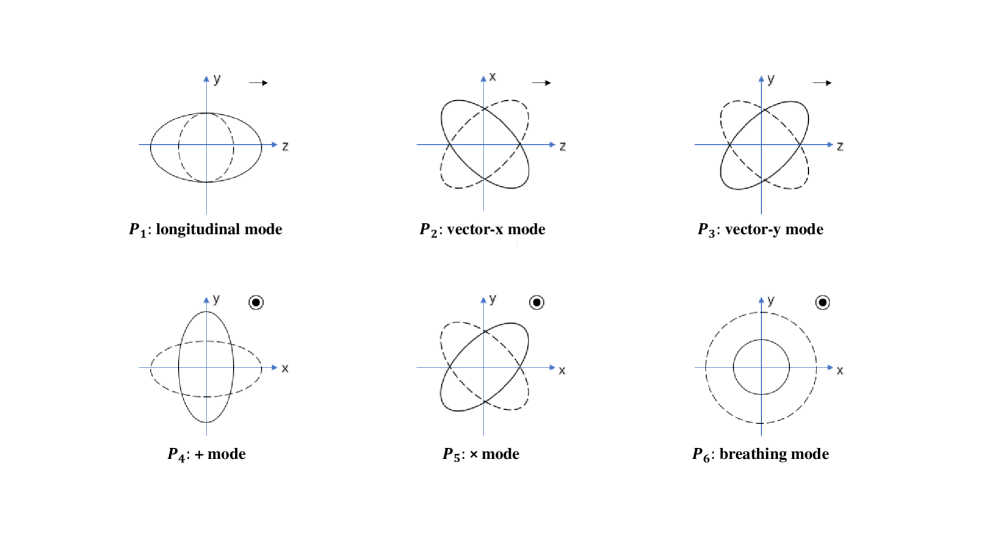
Figure 1: Six polarization modes of gravitational waves Eardley . We have assumed that the gravitational waves propagate in the $+z$ direction. The solid and dotted lines are the cases of a circle of test particles when the phases of waves are $0$ and $\pi$, respectively. There is no relative motion between test particles in the direction of the third axis that is not drawn.

Combining Eqs. (33) and (34), we can obtain the expressions of the six polarization modes

$$\begin{array}[]{l}P_{1}=\partial_{3}\partial_{3}\phi-\frac{1}{2}\partial_{0}\partial_{0}\Theta,\quad P_{2}=\frac{1}{2}\partial_{0}\partial_{3}\Xi_{1},\\ P_{3}=\frac{1}{2}\partial_{0}\partial_{3}\Xi_{2},\quad\quad\quad\quad\,\,P_{4}=-\frac{1}{2}\partial_{0}\partial_{0}h^{TT}_{11},\\ P_{5}=-\frac{1}{2}\partial_{0}\partial_{0}h^{TT}_{12},\quad\quad~{}~{}~{}P_{6}=-\frac{1}{2}\partial_{0}\partial_{0}\Theta.\end{array}$$ (38)

It can be seen that $h^{TT}_{ij}$ only contributes to tensor ($+$ and $\times$) modes, $\Xi_{i}$ only contributes to vector (vector-x and vector-y) modes, $\phi$ only contributes to longitudinal mode, and $\Theta$ contributes to both breathing mode and longitudinal mode.

Now, we will use the method introduced in Sec. IV to simplify the linear perturbation equations (12) and (13) and analyze the polarization modes of gravitational waves in generalized Proca theory in case (16).

V.1 Tensor mode

The equation describing the tensor mode gravitational waves can be derived from the transverse traceless tensor part of the $ij$ component in Eq. (13), which is

$$\left(\mathring{G}_{4}-\mathring{G}_{4,X}{A}^{2}\right)\partial_{0}\partial_{0}h^{TT}_{ij}-\mathring{G}_{4}\Delta h^{TT}_{ij}=0.$$ (39)

In order for generalized Proca theory to have tensor mode ($+$ and $\times$) gravitational waves, combining Eqs. (7) and (39), we should have the condition

$$\mathring{G}_{4}-\mathring{G}_{4,X}{A}^{2}\neq 0.$$ (40)

If the condition (40) is not satisfied, then Eq. (39) will become $\Delta h^{TT}_{ij}=0$. It indicates that $h^{TT}_{ij}$ has no wave solution, so this is not what we expected.

With the condition (40), we can obtain from Eq. (39) that the speed of the tensor mode gravitational waves $c_{T}$ is

$${c_{T}}^{2}=\frac{\mathring{G}_{4}}{\mathring{G}_{4}-\mathring{G}_{4,X}{A}^{2}}.$$ (41)

If ${c_{T}}^{2}\textless 0$, the solution will exponentially diverge, and then it is linearly unstable. To ensure the linear stability of the solution, we require ${c_{T}}^{2}\textgreater 0$.

GW170817 and GRB170817A require the speed of tensor mode gravitational waves $c_{T}$ to meet B.P.Abbott000 ; B.P.Abbott111

$$-3\times 10^{-15}\leq c_{T}-1\leq 7\times 10^{-16}.$$ (42)

This result will constrain the values of the theoretical parameters. Considering that Eq. (42) requires $c_{T}$ not to deviate significantly from the speed of light. Using Eq. (41), it shows that

$$\mid\mathring{G}_{4,X}{A}^{2}\mid\!\!\!~{}\ll\!\!\!~{}\mid\mathring{G}_{4}\mid.$$ (43)

Therefore, we can expand $c_{T}^{2}$ as

$$c_{T}^{2}\approx 1+\frac{\mathring{G}_{4,X}{A}^{2}}{\mathring{G}_{4}}.$$ (44)

Accordingly, $c_{T}$ has an approximation of

$$c_{T}\approx 1+\frac{\mathring{G}_{4,X}{A}^{2}}{2\mathring{G}_{4}}.$$ (45)

Therefore, it can be seen that the constrain (42) requires

$$\left|\frac{\mathring{G}_{4,X}{A}^{2}}{\mathring{G}_{4}}\right|\!\!~{}\lesssim\!\!~{}10^{-15}.$$ (46)

In particular, when the speed of tensor mode gravitational waves is strictly equal to the speed of light, we have $\mathring{G}_{4,X}=0$.

V.2 Vector mode

We can derive three equations describing vector mode gravitational waves from the linear perturbation equations (12) and (13).

The first equation can be derived from the transverse vector part of the $i$ component of Eq. (12), which is

$$\left(1-2c_{2}\mathring{G}_{4,X}\right)\Box\left(\Sigma_{i}+A\Xi_{i}\right)-\mathring{G}_{4,X}A\Delta\Xi_{i}=0.$$ (47)

The second and third equations can be derived respectively from the transverse vector parts of the $ij$ and $0i$ components of Eq. (13):

$$\mathring{G}_{4}\Xi_{i}+\mathring{G}_{4,X}A\Sigma_{i}=0,$$ (48)

$$\left(1-2c_{2}\mathring{G}_{4,X}\right)A\Box\left(\Sigma_{i}+A\Xi_{i}\right)-\mathring{G}_{4}\Delta\Xi_{i}-\mathring{G}_{4,X}A\Delta\left(\Sigma_{i}+A\Xi_{i}\right)=0.$$ (49)

Perhaps one would ask why there are only two variables $\Xi_{i}$, $\Sigma_{i}$ but three equations here. In fact, these three equations are not independent of each other. We can easily find that Eq. (49) can be obtained using Eqs. (47) and (48). Therefore, we only need to consider the first two.

Using Eq. (48), we have

$$\Xi_{i}=-\frac{\mathring{G}_{4,X}A}{\mathring{G}_{4}}\Sigma_{i}.$$ (50)

It can be seen that when $\mathring{G}_{4,X}=0$, we have $\Xi_{i}=0$. However, from Eq. (33), it can be seen that the gauge invariant vector that contributes to gravitational waves is only $\Xi_{i}$. Therefore, in this case, generalized Proca theory does not allow vector mode gravitational waves.

When $\mathring{G}_{4,X}\neq 0$, we can substitute Eq. (50) into Eq. (47), and obtain

$$\mathcal{M}\partial_{0}\partial_{0}\Sigma_{i}-\mathcal{N}\Delta\Sigma_{i}=0.$$ (51)

where

$$\mathcal{M} = \left(1-2c_{2}\mathring{G}_{4,X}\right)\left(\mathring{G}_{4}-\mathring{G}_{4,X}A^{2}\right),$$ (52)

$$\mathcal{N} = \mathcal{M}+{\mathring{G}_{4,X}}^{2}A^{2}.$$ (53)

This is an equation for the variable $\Sigma_{i}$. When we solve the wave solution of $\Sigma_{i}$ from Eq. (51), we can obtain $\Xi_{i}$ with Eq. (50), and then obtain the wave solution of vector mode gravitational waves. We already have the condition (40), so when considering $\mathring{G}_{4,X}\neq 0$, we can study this equation in the following three cases:

Case 1: When $1-2c_{2}\mathring{G}_{4,X}=0$, Eq. (51) becomes $\Delta\Sigma_{i}=0$. It indicates that $\Sigma_{i}$ has no wave solution, so we have $\Xi_{i}=\Sigma_{i}=0$. This case does not allow vector mode gravitational waves.

Case 2: When $\left(1-2c_{2}\mathring{G}_{4,X}\right)\left(\mathring{G}_{4}-\mathring{G}_{4,X}A^{2}\right)+{\mathring{G}_{4,X}}^{2}A^{2}=0$, Eq. (51) becomes $\partial_{0}\partial_{0}\Sigma_{i}=0$. It also indicates that $\Sigma_{i}$ has no wave solution, so we have $\Xi_{i}=\Sigma_{i}=0$. This case also does not allow vector mode gravitational waves.

Case 3: When $1-2c_{2}\mathring{G}_{4,X}\neq 0$ and $\left(1-2c_{2}\mathring{G}_{4,X}\right)\left(\mathring{G}_{4}-\mathring{G}_{4,X}A^{2}\right)+{\mathring{G}_{4,X}}^{2}A^{2}\neq 0$, Eq. (51) will have wave solutions of $\Sigma_{i}$. In this case, generalized Proca theory allows two vector (vector-x and vector-y) modes. Using Eq. (51), we obtain the speed of vector mode gravitational waves $c_{V}$:

$$c_{V}^{2}=1+\frac{{\mathring{G}_{4,X}}^{2}A^{2}}{\left(1-2c_{2}\mathring{G}_{4,X}\right)\left(\mathring{G}_{4}-\mathring{G}_{4,X}A^{2}\right)}.$$ (54)

Similar to the previous analysis of tensor modes, in order for the solution to have linear stability, we require $c_{V}^{2}\textgreater 0$. It can be seen that in Case 3, vector mode gravitational waves do not propagate at the speed of light, i.e. $c_{V}\neq 1$.

Based on the above research, we find that the existence of vector mode gravitational waves in generalized Proca theory depends on the parameter space. We summarize the results in Table 1.

Cases	Conditions	Vector DoF
case 0	$\mathring{G}_{4,X}=0.$	0
case 1	$\mathring{G}_{4,X}\neq 0,~{}1-2c_{2}\mathring{G}_{4,X}=0.$	0
case 2	$\mathring{G}_{4,X}\neq 0,~{}(1-2c_{2}\mathring{G}_{4,X})(\mathring{G}_{4}-\mathring{G}_{4,X}A^{2})+{\mathring{G}_{4,X}}^{2}A^{2}=0.$	0
case 3	$\mathring{G}_{4,X}\neq 0,~{}1-2c_{2}\mathring{G}_{4,X}\neq 0,~{}(1-2c_{2}\mathring{G}_{4,X})(\mathring{G}_{4}-\mathring{G}_{4,X}A^{2})+{\mathring{G}_{4,X}}^{2}A^{2}\neq 0.$	2

Table 1: The number of vector mode gravitational waves under various cases. The numbers in the rightmost column of the table represent the degrees of freedom of the vector mode gravitational waves in the corresponding case.

Finally, note that $\Xi_{i}$ in Eq. (50) depends on $\mathring{G}_{4,X}$, which allows us to use the speed of tensor mode gravitational waves to constrain the upper limit of the amplitude of vector mode gravitational waves.

First, all the perturbations are weak relative to the background:

$$\mid h_{ab}\mid\!\!\!~{}\ll\!\!\!~{}1,\quad\mid B^{a}\mid\!\!\!~{}\ll\!\!\!~{}\mid\mathring{A}^{a}\mid.$$ (55)

Then with Eqs. (25) and (IV), we have

$$\mid\Sigma_{i}\mid\!\!\!~{}\ll\!\!\!~{}\mid A\mid.$$ (56)

Therefore, using Eqs. (50) and (44), the condition (56) implies

$$\mid\Xi_{i}\mid\!\!\!~{}=\!\!\!~{}\left|\frac{\mathring{G}_{4,X}A}{\mathring{G}_{4}}\Sigma_{i}\right|\!\!\!~{}\ll\!\!\!~{}\left|\frac{\mathring{G}_{4,X}A^{2}}{\mathring{G}_{4}}\right|\!\!\!~{}\approx\!\!\!~{}\mid c_{T}^{2}-1\mid.$$ (57)

The above inequality gives the relationship between the vector mode amplitude and the tensor mode speed. Then, considering GW170817 and combining with the condition (46), we have from Eq. (57) that

$$\mid\Xi_{i}\mid\!\!\!~{}\ll\!\!\!~{}10^{-15}.$$ (58)

Using Eqs. (IV) and (25), the above constrain indicates that the metric perturbation (abbreviated as $h$) corresponding to the vector gravitational waves satisfy $|h|\ll 10^{-15}$. If we further require the speed of tensor modes to be the speed of light, i.e. $c_{T}=1$, then according to Eq. (57), we have $\Xi_{i}=0$. At this point, the amplitude of the vector modes is zero, and we can not detect the vector gravitational waves.

V.3 Scalar mode

We can derive six equations describing scalar mode gravitational waves from the linear perturbation equations (12) and (13).

The first and second equations can be derived from the $0$ component and the scalar part of the $i$ component of Eq. (12), respectively, which are given by

$$-2\left(1-2c_{2}\mathring{G}_{4,X}\right)\Delta\left(\Omega+2A\phi+\partial_{0}\Psi\right)+\mathring{G}_{3,X}A\left(2\Delta\Psi+3A\partial_{0}\Theta\right)$$

$$-4\mathring{G}_{4,X}A\Delta{\Theta}+2\mathring{G}_{2,XX}A^{2}\left(\Omega+A\phi\right)=0,$$ (59)

$$-\left(1-2c_{2}\mathring{G}_{4,X}\right)\partial_{0}\left(\Omega+2A\phi+\partial_{0}\Psi\right)-\mathring{G}_{3,X}A\left(\Omega+A\phi\right)-2\mathring{G}_{4,X}A\partial_{0}\Theta=0.$$ (60)

The third and fourth ones can be obtained respectively from the trace part and the $\partial_{i}\partial_{j}$ part of the $ij$ components of Eq. (13):

$$\mathring{G}_{4}\left(-4\Delta\phi-2\Delta\Theta+6\partial_{0}\partial_{0}\Theta\right)-3\mathring{G}_{3,X}A^{2}\partial_{0}\left(\Omega+A\phi\right)$$

$$-4\mathring{G}_{4,X}A\Delta\left(\Omega+A\phi+\partial_{0}\Psi\right)-6\mathring{G}_{4,X}A^{2}\partial_{0}\partial_{0}\Theta=0,$$ (61)

$$\mathring{G}_{4}\left(2\phi+\Theta\right)+2\mathring{G}_{4,X}A\left(\Omega+A\phi+\partial_{0}\Psi\right)=0.$$ (62)

Finally, the fifth and sixth equations can be derived respectively from the scalar part of the $0i$ component and the $00$ component of Eq. (13):

$$\left(1-2c_{2}\mathring{G}_{4,X}\right)A\left(\Omega+2A\phi+\partial_{0}\Psi\right)+2\mathring{G}_{4}\Theta=0,$$ (63)

$$4\left(1-2c_{2}\mathring{G}_{4,X}\right)A\Delta\left(\Omega+2A\phi+\partial_{0}\Psi\right)+4\mathring{G}_{4}\Delta\Theta+4\mathring{G}_{4,X}A^{2}\Delta\Theta$$

$$-\mathring{G}_{3,X}A^{2}\left(2\Delta\Psi+3A\partial_{0}\Theta\right)-2\mathring{G}_{2,XX}A^{3}\left(\Omega+A\phi\right)=0.$$ (64)

The above six equations are not independent of each other. Equation (V.3) can be obtained from Eqs. (V.3) and (63), and Equation (60) from Eqs. (V.3) and (62)(63). Therefore, only Eqs. (V.3) and (V.3)-(63) are independent. Now, we have four equations and four variables $\phi,\Theta,\Psi,\Omega$.

We can use Eqs. (V.3) and (62) to obtain the following equation:

$$2\left(\mathring{G}_{4}-\mathring{G}_{4,X}A^{2}\right)\partial_{0}\Theta-\mathring{G}_{3,X}A^{2}\left(\Omega+A\phi\right)=0.$$ (65)

This equation can replace Eq. (V.3), and we can solve scalar mode gravitational waves with Eqs. (V.3), (62), (63), and (65).

Now, we study scalar mode gravitational waves in the following four cases.

Case 1: $\mathring{G}_{3,X}=1-2c_{2}\mathring{G}_{4,X}=0$. In this case, using Eq. (40), we find that Eq. (65) requires $\Theta=0$. Thus Eq. (63) becomes

$$\left(1-2c_{2}\mathring{G}_{4,X}\right)A\left(\Omega+2A\phi+\partial_{0}\Psi\right)=0.$$ (66)

It can be seen that the equation is an identity. We now have only two equations (V.3) and (62) left to constrain the three variables $\phi,\Psi,\Omega$, which indicates that these variables can not be determined. So we do not consider this case.

Case 2: $\mathring{G}_{3,X}=0,\!~{}1-2c_{2}\mathring{G}_{4,X}\neq 0$. In this case, using Eq. (40), Eq. (65) also requires $\Theta=0$, while Eq. (63) requires

$$\Omega+2A\phi+\partial_{0}\Psi=0.$$ (67)

Then, from (62) we have

$$\left(\mathring{G}_{4}-\mathring{G}_{4,X}A^{2}\right)\phi=0.$$ (68)

Using Eq. (40), it requires $\phi=0$. Since $\Theta=\phi=0$, Eq. (33) indicates that scalar mode gravitational waves are not allowed in this case.

Case 3: $\mathring{G}_{3,X}\neq 0,\!~{}1-2c_{2}\mathring{G}_{4,X}=0$. In this case, using Eq. (63), we have $\Theta=0$. Then, Eq. (65) requires $\Omega+A\phi=0$. Using the above conditions, Eq. (V.3) will require $\Psi=0$. Finally, from Eq. (62), it can be seen that $\phi=0$. Since $\Theta=\phi=0$, scalar mode gravitational waves are not allowed in this case.

Case 4: $\mathring{G}_{3,X}\neq 0,\!~{}1-2c_{2}\mathring{G}_{4,X}\neq 0$. In this case, from Eq. (65) and (63), we have

$$\Omega+A\phi = \frac{2\left(\mathring{G}_{4}-\mathring{G}_{4,X}A^{2}\right)}{\mathring{G}_{3,X}A^{2}}\partial_{0}\Theta,$$ (69)

$$\Omega+2A\phi+\partial_{0}\Psi = -\frac{2\mathring{G}_{4}}{A\left(1-2c_{2}\mathring{G}_{4,X}\right)}\Theta.$$ (70)

Substituting Eq. (69) from Eq. (70) yields

$$A\phi+\partial_{0}\Psi=-\frac{2\mathring{G}_{4}}{A\left(1-2c_{2}\mathring{G}_{4,X}\right)}\Theta-\frac{2\left(\mathring{G}_{4}-\mathring{G}_{4,X}A^{2}\right)}{\mathring{G}_{3,X}A^{2}}\partial_{0}\Theta.$$ (71)

By substituting Eqs. (69) and (70) into Eq. (V.3), we obtain

$$\Delta\Psi=-\frac{2\left(\mathring{G}_{4}-\mathring{G}_{4,X}A^{2}\right)}{\mathring{G}_{3,X}A^{2}}\Delta\Theta-\frac{3{\mathring{G}_{3,X}}^{2}A^{2}+4\mathring{G}_{2,XX}\left(\mathring{G}_{4}-\mathring{G}_{4,X}A^{2}\right)}{2{\mathring{G}_{3,X}}^{2}A}\partial_{0}\Theta.$$ (72)

From Eqs. (71) and (72), it can be derived

$$\Delta\phi=\frac{3{\mathring{G}_{3,X}}^{2}A^{2}+4\mathring{G}_{2,XX}\left(\mathring{G}_{4}-\mathring{G}_{4,X}A^{2}\right)}{2{\mathring{G}_{3,X}}^{2}A^{2}}\partial_{0}\partial_{0}\Theta-\frac{2\mathring{G}_{4}}{A^{2}\left(1-2c_{2}\mathring{G}_{4,X}\right)}\Delta\Theta,$$ (73)

which gives the relationship between the amplitudes of the two scalar perturbations $\Theta$ and $\phi$ that affect scalar mode gravitational waves. Finally, with Eqs. (70) and (73), we obtain the equation for the variable $\Theta$ from Eq. (62):

$$\mathcal{P}\partial_{0}\partial_{0}\Theta-\mathcal{Q}\Delta\Theta=0.$$ (74)

where

$$\mathcal{P} = {\left(1-2c_{2}\mathring{G}_{4,X}\right)}{\left(\mathring{G}_{4}-\mathring{G}_{4,X}A^{2}\right)}\mathcal{C}_{1},$$ (75)

$$\mathcal{Q} = {{\mathring{G}_{3,X}}^{2}}\mathring{G}_{4}\mathcal{C}_{2},$$ (76)

$$\mathcal{C}_{1} = 3{\mathring{G}_{3,X}}^{2}A^{2}+4\mathring{G}_{2,XX}\left(\mathring{G}_{4}-\mathring{G}_{4,X}A^{2}\right),$$ (77)

$$\mathcal{C}_{2} = {4{\mathring{G}_{4}}-\left(1-2c_{2}\mathring{G}_{4,X}\right)A^{2}}.$$ (78)

We can further divide Case 4 into following cases.

Case 4.​​ 1: $\mathcal{C}_{1}=0,\!~{}\mathcal{C}_{2}=0$. In this case, we have

$$\Psi = -\frac{2\left(\mathring{G}_{4}-\mathring{G}_{4,X}A^{2}\right)}{\mathring{G}_{3,X}A^{2}}\Theta,$$ (79)

$$\phi = \frac{1}{2}\Theta.$$ (80)

We also have $\mathcal{P}=\mathcal{Q}=0$ and so we can not solve the function $\Theta$ with Eq. (74). Therefore, we do not consider this nonphysical case.

Case 4.​​ 2: $\mathcal{C}_{1}\neq 0,\!~{}\mathcal{C}_{2}=0$. In this case, Eq. (74) becomes $\partial_{0}\partial_{0}\Theta=0$. This requires $\Theta=0$, and then by Eq. (73), $\phi$ is also zero. Thus, generalized Proca theory does not allow scalar mode gravitational waves in this case.

Case 4.​​ 3: $\mathcal{C}_{1}=0,\!~{}\mathcal{C}_{2}\neq 0$. In this case, we have $\mathcal{P}=0$ and $\mathcal{Q}\neq 0$, which indicates that Eq. (74) becomes $\Delta\Theta=0$. This requires $\Theta=0$. And then by Eq. (73), $\phi$ is also zero. Therefore, generalized Proca theory does not allow scalar mode gravitational waves in this case either.

Case 4.​​ 4: $\mathcal{C}_{1}\neq 0,\!~{}\mathcal{C}_{2}\neq 0$. In this case, Eq. (74) is a wave equation and generalized Proca theory allows scalar mode gravitational waves with one degree of freedom. The speed of the scalar mode gravitational waves $c_{S}$ is

$$c_{S}^{2}=\frac{\mathcal{Q}}{\mathcal{P}}.$$ (81)

To ensure the linear stability of the solution, we require $c_{S}^{2}\textgreater 0$.

Finally, we consider a plane wave solution of $\Theta$ satisfying Eq. (74) with a propagation direction of $+z$:

$$\Theta=\Theta_{0}~{}\!e^{ikx},\quad\frac{k^{0}}{k^{3}}=c_{S}.$$ (82)

By substituting (82) into Eq. (73), we obtain

$$\Delta\phi=\left[-\frac{\mathcal{C}_{1}}{2{\mathring{G}_{3,X}}^{2}A^{2}}k_{0}^{2}+\frac{2\mathring{G}_{4}}{A^{2}\left(1-2c_{2}\mathring{G}_{4,X}\right)}k_{3}^{2}\right]\Theta_{0}~{}\!e^{ikx}.$$ (83)

Therefore, $\phi$ has a plane wave solution $\phi=\phi_{0}~{}\!e^{ikx}$ with

$$\phi_{0}=\left[\frac{\mathcal{C}_{1}}{2{\mathring{G}_{3,X}}^{2}A^{2}}c_{S}^{2}-\frac{2\mathring{G}_{4}}{A^{2}\left(1-2c_{2}\mathring{G}_{4,X}\right)}\right]\Theta_{0}.$$ (84)

Using Eq. (38), we have

$$P_{1} = \left[\frac{{\mathring{G}_{3,X}}^{2}A^{2}-\mathcal{C}_{1}}{2{\mathring{G}_{3,X}}^{2}A^{2}}k_{0}^{2}+\frac{2\mathring{G}_{4}}{A^{2}\left(1-2c_{2}\mathring{G}_{4,X}\right)}k_{3}^{2}\right]\Theta_{0}~{}\!e^{ikx};$$ (85)

$$P_{6} = \frac{1}{2}k_{0}^{2}\Theta_{0}~{}\!e^{ikx}.$$ (86)

So the amplitude ratio $\mathcal{R}$ of the longitudinal mode to the breathing mode is

$$\mathcal{R}=\left|\frac{P_{1}}{P_{6}}\right|=\left|\frac{{\mathring{G}_{3,X}}^{2}A^{2}-\mathcal{C}_{1}}{{\mathring{G}_{3,X}}^{2}A^{2}}+\frac{4\mathring{G}_{4}}{A^{2}\left(1-2c_{2}\mathring{G}_{4,X}\right){c_{S}}^{2}}\right|.$$ (87)

It can be seen that the scalar mode of generalized Proca theory is generally a mixture mode of the breathing and longitudinal modes. However, when $\mathcal{R}=0$, the scalar mode is just a pure breathing mode.

Based on the above research, we find that the existence of scalar mode gravitational waves in generalized Proca theory depends on the parameter spaces. We summarize the results in Table 2.

Cases	Conditions	Scalar DoF
case 1	$\mathring{G}_{3,X}=1-2c_{2}\mathring{G}_{4,X}=0$.	-
case 2	$\mathring{G}_{3,X}=0,\!~{}1-2c_{2}\mathring{G}_{4,X}\neq 0$.	0
case 3	$\mathring{G}_{3,X}\neq 0,\!~{}1-2c_{2}\mathring{G}_{4,X}=0$.	0
case 4.​​ 1	$\mathring{G}_{3,X}\neq 0,\!~{}1-2c_{2}\mathring{G}_{4,X}\neq 0,\!~{}\mathcal{C}_{1}=0,\!~{}\mathcal{C}_{2}=0$.	-
case 4.​​ 2	$\mathring{G}_{3,X}\neq 0,\!~{}1-2c_{2}\mathring{G}_{4,X}\neq 0,\!~{}\mathcal{C}_{1}\neq 0,\!~{}\mathcal{C}_{2}=0$.	0
case 4.​​ 3	$\mathring{G}_{3,X}\neq 0,\!~{}1-2c_{2}\mathring{G}_{4,X}\neq 0,\!~{}\mathcal{C}_{1}=0,\!~{}\mathcal{C}_{2}\neq 0$.	0
case 4.​​ 4	$\mathring{G}_{3,X}\neq 0,\!~{}1-2c_{2}\mathring{G}_{4,X}\neq 0,\!~{}\mathcal{C}\neq 0,\!~{}\mathcal{C}_{2}\neq 0$.	1

Table 2: The number of scalar mode gravitational waves in various parameter spaces. The number in the rightmost column of the table represents the degrees of freedom of the scalar mode gravitational waves in the corresponding case. The notation ”-” indicates that the parameter space is not physical.

VI Conclusion

In this paper, under the background of the homogeneous and isotropic Minkowski space-time, we study the polarization modes of gravitational waves in generalized Proca theory under linearized perturbations. We first obtained the background equations and the linear perturbation equations. Then we analyzed the polarization modes of gravitational waves and discussed their linear stability.

We found that the polarization modes of gravitational waves in generalized Proca theory depend on the parameter spaces. There are different vector and scalar polarization modes in different parameter spaces. The specific results have been summarized in Table 1 and Table 2, respectively. Generalized Proca theory allows at most two tensor modes, two vector modes and one scalar mode. The scalar mode is typically a mixture mode of the breathing and longitudinal modes. However, when $\mathcal{R}$ in Eq. (15) is zero, then the scalar mode is just a pure breathing mode.

We also found that the amplitude of vector mode gravitational waves satisfies the condition (57). This allows us to give the upper limit of the amplitude of vector mode gravitational waves by detecting the speed of tensor mode gravitational waves. Combining the results of GW170817, we found that the amplitude of vector gravitational waves has an upper bound of $|h|\ll 10^{-15}$. It should be noted that as the speed of tensor gravitational waves approaches the speed of light, the upper bound of the amplitude of vector gravitational waves decreases. Specifically, if the speed of tensor modes is strictly equal to the speed of light, then the amplitude of vector modes is zero.

Finally, we need to point out that we only considered the case of the homogeneous and isotropic Minkowski background. At this point, the background vector $\mathring{A}_{a}$ has only a nonvanishing timporal component. In the case of a small anisotropic background, the background vector $\mathring{A}_{a}$ also has nonvanishing small spatial components. In this case, the background vector is time-like. We can always use a Lorentz transformation to make the background vector have only nonvanishing temporal component without losing generality. It can be seen that the polarization modes of gravitational waves in the anisotropic case can be directly obtained by using the Lorentz transformation on the polarization modes of gravitational waves in the isotropic case we have studied. For a general discussion of the transformation law of the polarization modes of gravitational waves under the Lorentz transformation, one can refer to Ref. Y.Liu .

The polarization modes of gravitational waves in generalized Proca theory can be divided into quite rich cases by parameter spaces. The appropriate parameter spaces can be expected to be selected in the detection of gravitational wave polarization modes by Lisa, Taiji and TianQin lisa ; taiji ; tianqin in the future.

References

• (1) B. P. Abbott et al. (LIGO Scientific Collaboration and Virgo Collaboration), “Observation of Gravitational Waves from a Binary Black Hole Merger”, Phys. Rev. Lett. 116, 061102 (2016).
• (2) B. P. Abbott et al. (LIGO Scientific Collaboration and Virgo Collaboration), “GW151226: Observation of Gravitational Waves from a 22-Solar-Mass Binary Black Hole Coalescence”, Phys. Rev. Lett. 116, 241103 (2016).
• (3) B. P. Abbott et al. (LIGO Scientific Collaboration and Virgo Collaboration), “GW170104: Observation of a 50-Solar-Mass Binary Black Hole Coalescence at Redshift 0.2”, Phys. Rev. Lett. 118, 221101 (2017).
• (4) B. P. Abbott et al. (LIGO Scientific Collaboration and Virgo Collaboration), “GW170814: A Three-Detector Observation of Gravitational Waves from a Binary Black Hole Coalescence”, Phys. Rev. Lett. 119, 141101 (2017).
• (5) B. P. Abbott et al. (LIGO Scientific Collaboration and Virgo Collaboration), “GW170817: Observation of Gravitational Waves from a Binary Neutron Star Inspiral”, Phys. Rev. Lett. 119, 161101 (2017).
• (6) S. Pi, “Detecting warm dark matter by the stochastic gravitational waves”, Sci. China Phys. Mech. Astron. 64, 290431 (2021).
• (7) A, Addazi, Y. Cai, Q. Gan, A. Marciano and K. Zeng, “NANOGrav results and dark first order phase transitions”, Sci. China Phys. Mech. Astron. 64, 290411 (2021).
• (8) R. Cai, “A diffraction phenomenon of gravitational waves:Poisson-Arago spot for gravitational waves”, Sci. China Phys. Mech. Astron. 64, 120461 (2021).
• (9) Z. Zhao and Z. Cao, “Stochastic gravitational wave background due to gravitational wave memory”, Sci. China Phys. Mech. Astron. 65, 119511 (2022).
• (10) Z. Guo, “Standard siren cosmology with the LISA-Taiji network”, Sci. China Phys. Mech. Astron. 65, 210431 (2022).
• (11) R. Cai, Z. Cao, Z. Guo, S. Wang and T. Yang, “The gravitational-wave physics”, Natl. Sci. Rev. 4, 687 (2017).
• (12) L. Bian, R. Cai, S. Cao, Z. Cao, H. Gao et al. “The Gravitational-wave physics II: Progress”, Sci. China Phys. Mech. Astron. 64, 120401 (2021).
• (13) D. M. Eardley, D. L. Lee and A. P. Lightman, “Gravitational-wave observations as a tool for testing relativistic gravitye”, Phys. Rev. D 8, 3308 (1973).
• (14) D. Liang, Y. Gong, S. Hou and Y. Liu, “Polarizations of gravitational waves in $f(R)$ gravity”, Phys. Rev. D 95, 104034 (2017).
• (15) S. Hou, Y. Gong and Y. Liu, “Polarizations of gravitational waves in Horndeski theory”, Eur. Phys. J. C 78, 378 (2018).
• (16) Y. Gong, S. Hou, D. Liang and E. Papantonopoulos, “Gravitational waves in Einstein-ather and generalized TeVeS theory after GW170817”, Phys. Rev. D 97, 084040 (2018).
• (17) Y. Gong, S. Hou, E. Papantonopoulos and D. Tzortzis, “Gravitational waves and the polarizations in Horava gravity after GW170817”, Phys. Rev. D 98, 104017 (2018).
• (18) Y. Liu, W. Qian, Y. Gong and B. Wang, “Gravitational waves in scalar-tensor-vector gravity theory”, Universive 7, 9 (2021).
• (19) K. Bamba, S. Capozziello, M. D. Laurentis, S. Nojiri and D. Saez-Gomez, “No further gravitational wave modes in $f(T)$ gravity”, Phys. Lett. B 727, 194 (2013).
• (20) P. Wagle, A. Saffer and N. Yunes, “Polarization modes of gravitational waves in quadratic gravity”, Phys. Rev. D 100, 124007 (2019).
• (21) Y. Dong and Y. Liu, “Polarization modes of gravitational waves in Palatini-Horndeski theory”, Phys. Rev. D 105, 064035 (2022).
• (22) S. Bahamonde, and M. Hohmann, M. Caruana, K. F. Dialektopoulos, V. Gakis, J. LeviSaid, E. N. Saridakis and J. Sultana, “Gravitational-wave propagation and polarizations in the teleparallel analog of Horndeski gravity”, Phys. Rev. D 104, 084082 (2021).
• (23) J. Lu, J. Li, H. Guo, Z. Zhuang and X. Zhao, “Linearized physics and gravitational-waves polarizations in the Palatini formalism of GBD theory”, Phys. Lett. B 811, 135985 (2020).
• (24) D. Liang, R. Xu, X. Lu and L. Shao, “Polarizations of Gravitational Waves in the Bumblebee Gravity Model”, Phys. Rev. D 106, 124019 (2022).
• (25) H. Takeda, S. Morisaki, and A. Nishizawa, “Pure polarization test of GW170814 and GW170817 using waveforms consistent with modified theories of gravity”, Phys. Rev. D. 103, 064037 (2021).
• (26) B. P. Abbott et al. (LIGO Scientific Collaboration and Virgo Collaboration), “Search for Tensor, Vector, and Scalar Polarizations in the Stochastic Gravitational-Wave Background”, Phys. Rev. Lett. 120, 201102 (2018).
• (27) B. P. Abbott et al. (LIGO Scientific Collaboration and Virgo Collaboration), “Search for the isotropic stochastic background using data from Advanced LIGO’s second observing run”, Phys. Rev. D. 100, 061101(R) (2019).
• (28) B. P. Abbott et al. (LIGO Scientific Collaboration and Virgo Collaboration), “Tests of general relativity with binary black holes from the second LIGO-Virgo gravitational-wave transient catalog”, Phys. Rev. D. 103, 122002 (2021).
• (29) A. Nishizawa, A. Taruya, K. Hayama, S. Kawamura, and M. A. Sakagami, “Probing nontensorial polarizations of stochastic gravitational-wave backgrounds with ground-based laser interferometers”, Phys. Rev. D 79, 082002 (2009).
• (30) K. Hayama and A. Nishizawa, “Model-independent test of gravity with a network of ground-based gravitational-wave detectors”, Phys. Rev. D 87, 062003 (2013).
• (31) M. Isi, A. J. Weinstein, C. Mead and M. Pitkin, “Detecting beyond-Einstein polarizations of continuous gravitational waves”, Phys. Rev. D 91, 082002 (2015).
• (32) M. Isi, M. Pitkin and A. J. Weinstein, “Probing dynamical gravity with the polarization of continuous gravitational waves”, Phys. Rev. D 96, 042001 (2017).
• (33) K. Chatziioannou, N. Yunes and N. Cornish, “Model-independent test of general relativity: An extended post-Einsteinian framework with complete polarization content”, Phys. Rev. D 86, 022004 (2012) [Erratum: Phys. Rev. D 95, 129901(E) (2017)]
• (34) H. Takeda, A. Nishizawa, Y. Michimura, K. Nagano, K. Komori, M. Ando and K. Hayama, “Polarization test of gravitational waves from compact binary coalescences”, Phys. Rev. D 98, 022008 (2018).
• (35) Y. Hagihara, N. Era, D. Iikawa, and H. Asada, “Probing gravitational wave polarizations with Advanced LIGO, Advanced Virgo, and KAGRA”, Phys. Rev. D 98, 064035 (2018).
• (36) P. T. H. Pang, R. K. L. Lo, I. C. F. Wong, T. G. F. Li, and C. VanDenBroeck, “Generic searches for alternative gravitational wave polarizations with networks of interferometric detectors”, Phys. Rev. D 101, 104055 (2020).
• (37) B. P. Abbott et al. (LIGO Scientific Collaboration and Virgo Collaboration), “First Search for Nontensorial Gravitational Waves from Known Pulsars”, Phys. Rev. Lett. 120, 031104 (2018).
• (38) Y. Jing, “The dawn of a new era of pulsar discoveries by Chinese radio telescope FAST”, Sci. China Phys. Mech. Astron. 64, 129561 (2021).
• (39) Z. Chen, C. Yuan and Q. Huang, “Non-tensorial gravitational wave background in NANOGrav 12.5-year data set”, Sci. China Phys. Mech. Astron. 64, 120412 (2021).
• (40) P. Amaro-Seoane, H. Audley, S. Babak and et al. (LISA Team), “Laser interferometer space antenna”, eprint arXiv:1702.00786.
• (41) Z. Luo, Y. Wang, Y. Wu, W. Hu and G. Jin, “The Taiji program: A concise overview”, Prog. Theor. Exp. Phys. 2021, 05A108 (2021).
• (42) G. Wang and W. B. Han, “Observing gravitational wave polarizations with the LISA-TAIJI network”, Phys. Rev. D. 103, 064021 (2021).
• (43) J. Luo, L. S. Chen, H. Z. Duan et al., “TianQin: A space-borne gravitational wave detector”, Classical. Quant. Grav. 33, 035010 (2016).
• (44) A. A. Starobinsky, “A New Type of Isotropic Cosmological Models Without Singularity”, Phys. Lett. B 91, 99 (1980).
• (45) K. Sato, “First Order Phase Transition of a Vacuum and Expansion of the Universe”, Mon. Not. Roy. Astron. Soc. 195, 467 (1981).
• (46) A. H. Guth, “The Inflationary Universe: A Possible Solution to the Horizon and Flatness Problems”, Phys. Rev. D 23, 347 (1981).
• (47) L. Heisenberg, “A systematic approach to generalisations of General Relativity and their cosmological implications”, Phys.Rept. 796, 1 (2019).
• (48) G. W. Horndeski, “Second-order scalar-tensor field equations in a four-dimensional space”, Int. J. Theor. Phys. 10, 363 (1974).
• (49) A. Nicolis, R. Rattazzi and E. Trincherini, “Galileon as a local modification of gravity”, Phys. Rev. D 79, 064036 (2009).
• (50) C. Deffayet, G. Esposito-Farese and A. Vikman, “Covariant Galileon”, Phys. Rev. D 79, 084003 (2009).
• (51) C. Deffayet, X. Gao, D. A. Steer and G. Zahariade, “From k-essence to generalized Galileons”, Phys. Rev. D 84, 064039 (2011).
• (52) L. Heisenberg, “Generalization of the Proca Action”, J. Cosmol. Astropart. Phys. 05, 015 (2014).
• (53) M. Ostrogradsky, “Memoires sur les equations differentielle relatives au probleme des isoperimetres”, Mem. Ac. St. Petersbourg VI 4, 385 (1850).
• (54) A. D. Felice, L. Heisenberg, R. Kase, S. Mukohyama, S. Tsujikawa and Y. Zhang, “Cosmology in generalized Proca theories”, J. Cosmol. Astropart. Phys. 06, 048 (2016).
• (55) L. Heisenberg, R. Kase and S. Tsujikawa, “Anisotropic cosmological solutions in massive vector theories”, J. Cosmol. Astropart. Phys. 11, 008 (2016).
• (56) C. Geng, Y. Hsu, J. Lu and L. Yin, “A dark energy model from generalized Proca theory”, Phys.Dark Univ. 32, 100819 (2021).
• (57) E. Babichev, C. Charmousis and M. Hassaine, “Black holes and solitons in an extended Proca theory”, J. High Energy Phys. 05, 114 (2017).
• (58) L. Heisenberg, R. Kase, M. Minamitsuji and S. Tsujikawa, “Hairy black-hole solutions in generalized Proca theories”, Phys. Rev. D 96, 084049 (2017).
• (59) L. Heisenberg, R. Kase, M. Minamitsuji and S. Tsujikawa, “Black holes in vector-tensor theories”, J. Cosmol. Astropart. Phys. 08, 024 (2017).
• (60) S. Garcia-Saenz, A. Held and J. Zhang, “Destabilization of Black Holes and Stars by Generalized Proca Fields”, Phys. Rev. Lett. 127, 131104 (2021).
• (61) A. D. Felice, L. Heisenberg, R. Kase, S. Tsujikawa, Y. Zhang and G. Zhao, “Screening fifth forces in generalized Proca theories”, Phys. Rev. D 93, 104016 (2016).
• (62) R. Jackiw and S. Pi, “Chern-Simons modification of general relativity”, Phys. Rev. D 68, 104012 (2003).
• (63) E. E. Flanagan and S. A. Hughes, “The basics of gravitational wave theory”, New J. Phys. 7, 204 (2005).
• (64) S. Weinberg, “Cosmology”, (Oxford University Press, 2008).
• (65) R. Bluhm, S. Fung and V. A. Kostelecky, “Spontaneous Lorentz and diffeomorphism violation, massive modes, and gravity”, Phys. Rev. D 77, 065020 (2008).
• (66) C. W. Misner, K. S. Thorne and J. A. Wheeler, “Gravitation”, (Princeton University Press, 1973).
• (67) B. P. Abbottet et al. (LIGO Scientific Collaboration and Virgo Collaboration), “Gravitational waves and gamma-rays from a binary neutron star merger: GW170817 and GRB 170817A”, Astrophys. J. 848, L13 (2017).
• (68) B. P. Abbottet et al. (LIGO Scientific Collaboration and Virgo Collaboration), “Tests of General Relativity with GW170817”, Phys. Rev. Lett. 123, 011102 (2019).
• (69) Y. Liu, Y. Dong and Y. Liu, “Classification of Gravitational Waves in Higher-dimensional Space-time and Possibility of Observation”, eprint arXiv:2206.15333.