Majorana Thermoelectrics and Refrigeration

Abstract

A two-terminal quantum spin-Hall heat engine and refrigerator with embedded Majorana bound states (MBS) are analyzed for optimality in thermoelectric performance. The occurrence of MBS can enhance the performance to rival, as well as outperform, some modern nanoscale quantum heat engines and quantum refrigerators. The optimal performance of this MBS quantum heat engine and quantum refrigerator can be further enhanced by an Aharonov-Bohm flux.

I Introduction

Majorana fermions are quasiparticle excitations that possess non-Abelian statistics and are predicted to exist in certain topological superconductors. These fermions have attracted significant interest due to their potential applications in quantum computing and topological quantum technologies. They are a unique class of fermions with the unusual property of being anti-particles. They could be used to encode information in qubits immune to decoherence [1, 2]. This property makes Majorana fermions invaluable for the construction of quantum computers. The potential application of Majorana fermions in the design of quantum heat engines and quantum refrigerators has been explored rarely, although the figure of merit has been discussed [3].

Heat engines convert generated heat into practical work, while refrigerators cause heat to flow from a colder terminal to a hotter terminal by utilizing energy or input work. The generation of excess heat in nanoscale devices is a problem that has received considerable attention. This excess heat is either wasted or damages the device. Thermoelectric effects in mesoscopic systems [4, 5, 6, 7] can be used to design nanoscale heat engines [4, 8, 9, 10] that can be used as a conduit to alter the excess heat generated into practical work [6, 11]. We propose a setup that can act as a steady-state heat engine [12, 11] or as a steady-state refrigerator [13, 14, 15] in distinct parameter regimes.

In the context of a two-terminal quantum spin-Hall heat engine and refrigerator, Majorana bound states(MBS) formed due to interacting Majorana fermions can improve thermoelectric performance. Thermoelectric devices convert temperature gradients into electrical energy or vice versa using the Seebeck and Peltier effects. The utilization of MBS in such devices can enhance their efficiency. Furthermore, introducing an Aharonov-Bohm flux can provide additional control over the system’s performance. The Aharonov-Bohm effect is a quantum phenomenon that arises when charged particles are influenced by a magnetic field, even when confined to regions with zero magnetic field strength. By manipulating the Aharonov-Bohm flux, one can modulate the behavior of the Majorana bound states and potentially optimize the performance of the quantum heat engine and refrigerator.

This paper studies a two-terminal quantum spin Hall-based Aharonov-Bohm interferometer with embedded Majorana bound states (MBS). We study thermoelectric transport in the presence of MBS by calculating the figure of merit, maximum efficiency, maximum power, and the corresponding efficiency at maximum power for a quantum heat engine and the coefficient of performance (COP) and cooling power for a quantum refrigerator. We show that in the presence of MBS (coupled or individual), the device’s performance as a quantum heat engine and quantum refrigerator is significantly improved. We also show that coupling between individual MBS, as well as the coupling between MBS and the interferometer arms, can significantly affect performance. Tuning the Aharonov-Bohm flux can greatly improve the performance of our setup to match or even outperform other contemporary quantum heat engines and refrigerators[11, 10, 13, 14]. For high output power, the corresponding efficiency is low; similarly, for high cooling power, the corresponding coefficient of performance is very low. For our proposed quantum spin Hall heat engine/refrigerator to be viable, it must have a high efficiency with finite output power and a high coefficient of performance with finite cooling power. This paper seeks to find such optimal parameter regimes wherein this is possible.

The rest of the paper is organized as follows: In section II, we discuss thermoelectric transport in mesoscopic systems and calculate the various thermoelectric parameters that can be used to quantify the performance of the system as a heat engine or refrigerator using the Onsager relations [16, 5]. Section III discusses our proposed Aharonov-Bohm interferometer (ABI) and calculates the transmission probability in the presence of MBS using Landauer-Buttiker scattering theory [17]. In section IV, we study the effect of MBS on the setup’s performance as a quantum heat engine and as a quantum refrigerator. We present our results and analysis in section V and end with the conclusions in section VI.

II Theory of Thermoelectric Transport in quantum spin hall setups

The proposed setup is a two-terminal quantum spin Hall ABI. We explain the thermoelectric transport in our setup using Onsager relations [5] and Landauer-Buttiker scattering theory [17]. We denote current by vector $I^{s}=(I^{s}_{c},I^{s}_{q}),$ where $I^{s}_{c}=I^{s}_{e,c}+I^{s}_{h,c}$ is the total charge current for spin $s\in(\uparrow,\downarrow)$ electrons and holes and $I^{s}_{q}=I^{s}_{e,q}+I^{s}_{h,q}$ total the heat current for spin $s$ electrons and holes. $F=(\Delta V,\Delta T)$ is the thermodynamic force vector, where $\Delta V$ is the voltage bias, and $\Delta T$ is the temperature difference across the two reservoirs. The total current vector $I=(I_{c}^{\uparrow}+I_{c}^{\downarrow},I_{q}^{\uparrow}+I_{q}^{\downarrow})$ can be related to force vector $F=(\Delta V,\Delta T)$ by the Onsager matrix $L$ such that $I=LF$, where [5, 4],

and $f(E,E_{F})$ being the Fermi function, with

$T$ is the temperature, $k_{B}$ is the Boltzmann constant, $G_{0}=(e^{2}/\hbar)$ is the conductance quantum, $E$ is particle energy, $E_{F}$ is Fermi energy, and $h$ is Planck’s constant. $\mathcal{T}=\sum_{s,r,k}T^{sr}_{k}$ is the total transmission probability for an electron of spin $r$ incident from the left to transmit as an electron or hole ($k=e,h$) with spin $s$. Since the opposite spin edge modes are mirror images of each other and there is no spin-flip scattering in our system (see Fig. 1), we can write $\mathcal{T}^{\uparrow\uparrow}_{k}=\mathcal{T}^{\downarrow\downarrow}_{k}$, and $\mathcal{T}^{\uparrow\downarrow}_{k}=\mathcal{T}^{\uparrow\downarrow}_{k}=0$. From Eq. 1, we can write [16]:

$$I_{c}=L_{cV}\Delta V+L_{cT}\Delta T\text{ and }I_{q}=L_{qV}\Delta V+L_{qT}\Delta T.$$ (4)

The second law of thermodynamics states that the total entropy must increase in any thermodynamic process. Since the total entropy increases, the entropy production rate $\dot{\xi}$ given by,

$$\dot{\xi}=I_{c}\Delta V+I_{q}\Delta T,$$ (5)

must be positive. The positivity of entropy production [16] rate implies

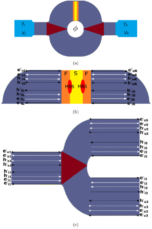
Figure 1: (a) The proposed MBS-ABI quantum heat engine/quantum refrigerator. It is a 2D TI ring with helical edge modes flowing in the outer and inner edges. The ring is coupled to two leads via couplers (shown in brown). The leads connect the AB ring to reservoirs at temperatures $T_{L}$ and $T_{R}$, and voltages $V_{L}$ and $V_{R}$. The ring is pierced by an Aharonov-Bohm flux. Ferromagnetic (shown in orange) and superconducting (shown in yellow) correlations are induced in the top arm of the ring via the proximity effect. (b) The superconductor-topological insulator-ferromagnet (STIM) junction. MBS (shown as red ellipses) occurs at the interface of the ferromagnetic (shown in orange) and superconducting (shown in yellow) layer. (c) Scattering of the edge modes at the left coupler. The solid and dashed lines represent the electron and hole edge modes. The black and white lines represent the spin-up and spin-down edge modes. The double-headed arrows represent the outer edge modes, and the single-headed arrows represent the inner edge modes, respectively.

$$\begin{split}L_{cV}\geq 0,L_{qT}\geq 0,L_{cV}L_{qT}-\dfrac{1}{4}(L_{cT}+L_{qV})^{2}\geq 0.\end{split}$$ (6)

The output power [16] is given by,

$$P=I_{c}\Delta V=(L_{cV}\Delta V+L_{cT}\Delta T)\Delta V\,.$$ (7)

For $\Delta T>0$ and $\Delta V>0$, a current is driven through the system such that output power is positive and the system behaves as a quantum heat engine. We can maximize the output power by finding $\Delta V$ such that $\dfrac{dP}{d\Delta V}=0$. For maximum power, we find the voltage bias

$$\Delta V=-\dfrac{L_{cT}}{2L_{cV}}\Delta T.$$ (8)

Substituting $\Delta V$ from Eq. (8) in Eq. (7), we obtain the maximum power

$$P_{max}=\dfrac{1}{4}\dfrac{(L_{cT})^{2}(\Delta T)^{2}}{L_{cV}}\,,$$ (9)

and the corresponding efficiency at maximum power [16] is given by,

$$\eta_{maxP}=\dfrac{P_{max}}{I_{q}}=\dfrac{\eta_{c}T}{2}\dfrac{L_{cT}^{2}}{2L_{cV}L_{qT}-L_{cT}L_{qV}}\,,$$ (10)

From Eqs. (4, 7), we can write the efficiency [16] $\eta$ as,

$$\eta=\dfrac{P}{I_{q}}=\dfrac{(L_{cV}\Delta V+L_{cT}\Delta T)\Delta V}{L_{qV}\Delta V+L_{qT}\Delta T},$$ (11)

or

$$\eta=\dfrac{-(\Delta V-S\Delta T)\Delta V}{TS\Delta V-(\dfrac{\kappa}{\sigma}+TS^{2})\Delta T)},$$ (12)

wherein $\sigma=L_{cV}$ is the electrical conductance, $\kappa$ is the thermal conductance [13] given by,

$$\kappa=\dfrac{I_{q}}{\Delta T}|_{I_{c}=0}=\dfrac{L_{cV}L_{qT}-L_{cT}L_{qV}}{L_{cV}},$$ (13)

and $S=\dfrac{-L_{cT}}{L_{cV}}$ is the Seebeck coefficient [13]. Similarly, we can maximize $\eta$ by taking $\Delta V$ such that $\dfrac{d\eta}{d\Delta V}=0$ in Eq. (11) with the condition $I_{q}>0$ [16, 11] to give us maximum efficiency,

$$\eta_{max}=\eta_{c}\dfrac{\sqrt{Z_{T}+1}-1}{\sqrt{Z_{T}+1}+1}.$$ (14)

where $\eta_{c}=\Delta T/T$ is the Carnot efficiency and $Z_{T}$ the figure of merit [16, 11, 3] given as,

$$Z_{T}=\sigma\dfrac{S^{2}}{\kappa}eT\,.$$ (15)

For the system to work as a quantum refrigerator, net heat current must flow from the cooler to the hotter terminal as net electrical current flows from the higher to the lower potential. The coefficient of performance (COP) is defined as the ratio of heat current ($I_{q}$) absorbed to electrical power ($P$) applied and is given as,

$$COP=\eta^{r}=I_{q}/P,$$ (16)

where $I_{q}$ is the heat current extracted. Thus, $I_{q}<0$, which implies that for the system to work as a refrigerator, $P<0$, maximum COP [13] is,

$$\eta_{max}^{r}=\eta_{c}^{r}\dfrac{\sqrt{Z_{T}+1}-1}{\sqrt{Z_{T}+1}+1},$$ (17)

where $\eta_{c}^{r}=T/\Delta T$. The corresponding cooling power at the maximum coefficient of performance is then given as[13]

$$P^{r}_{max}=\Delta T\sqrt{\dfrac{L_{qT}(L_{cV}L_{qT}-L_{cT}L_{qV})}{L_{cV}}}.$$ (18)

In the absence of spin-flip scattering, transmission probabilities of spin-up electrons/holes are the same as the transmission probabilities of spin-down electrons/holes, i.e., $\mathcal{T}^{\uparrow\uparrow}=\mathcal{T}^{\downarrow\downarrow}$ and the net spin transport is zero. The following section discusses the proposed setup and calculates the scattering amplitudes to find the transmission probability $\mathcal{T}$. The transmission probability can be plugged in Eq. (1) to find the Onsager coefficients, $L_{cV},L_{qV},L_{cT},L_{qT}$ and the rest of the thermoelectric parameters in Eqs. (9-18).

III Model

III.1 Hamiltonian

Our proposed quantum heat engine/refrigerator works based on helical edge modes generated via the quantum spin Hall effect in topological insulators (TIs). We mould a 2D TI into an Aharonov-Bohm ring wherein spin-orbit coupling generates protected 1D edge modes. In Fig. 1, we show our proposed model. The ring is pierced by an Aharonov-Bohm flux $\phi$. Couplers connect the ring to the leads, which are then connected to two reservoirs at temperatures $T_{L}$ and $T_{R}$, and voltages $V_{L}$ and $V_{R}$, respectively. The Dirac equation for electrons and holes in the ring is given as

$$[vp\tau_{z}\sigma_{z}+(-E_{F}+eA/(\hbar c))\tau_{z}]\psi=E\psi\,.$$ (19)

$\psi$ is a four-component spinor given by $\psi=(\psi_{e\uparrow},\psi_{e\downarrow},\psi_{h\downarrow},\psi_{h\uparrow})^{T}$, $p=-i\hbar\partial/\partial x$ is the momentum operator, $E_{F}$ is the Fermi energy, $E$ is the incident electron energy, $v_{F}$ is the Fermi velocity, and $A$ is the magnetic vector potential. MBS (shown in red) occur in the upper half of the ring at the junction between the superconducting and ferromagnetic layer in the TI (STIM junction) (see Fig. 1) [18, 19, 20]. The Hamiltonian for the MBS is [21, 20]

$$H_{M}=-\sigma_{y}E_{M}\,,$$ (20)

with $E_{M}$ denoting coupling strength between individual MBS. The STIM junction is connected to the left and right arms of the ring with coupling strengths $\Gamma_{1}$ and $\Gamma_{2}$, respectively. In the next subsection, we outline the scattering via edge modes in the setup and calculate the transmission probability $\mathcal{T}$.

III.2 Transport in the system via edge modes

In a simple quantum Hall ring with an Aharonov-Bohm flux, localized flux-sensitive edge modes develop near the hole, while in leads, edge modes are insensitive to flux [21]. To tune the device with an Aharonov-Bohm flux, we must couple the edge modes in the leads and the edge modes in the ring to make the net conductance flux-sensitive. It can be achieved via couplers in the system that can couple the inner and outer edge modes via inter-edge scattering and backscattering. The STIM junction at the top of the ring generates MBS and acts as a backscatter, mixing the electron and hole edge modes. Considering the electron and hole edge modes of spins up and down, we get eight edge modes, with four edge modes circulating on the outer edge and four edge modes circulating on the inner edge. Since no spin-flip scattering takes place in our setup, we can significantly simplify the calculation by dividing the edge modes into two sets of edge modes of opposite spin that scatter as mirror images. It allows us to calculate the transmission for a single set and double it to get the net conductance.
The first set consists of the spin-up electron and spin-up hole edge modes. The second set consists of a counterpropagating spin-down electron and spin-down hole edge modes. The STIM junction couples the incoming and outgoing edge modes of each set. Among the spin-up edge modes, incoming edge modes into the STIM junction are given by $I_{MBS1}=(e^{\uparrow}_{oL},e^{\uparrow}_{iR},h^{\uparrow}_{oL},h^{\uparrow}_{iR})$ and the outgoing edge modes are given by $O_{MBS1}=(e^{\uparrow}_{oR},e^{\uparrow}_{iL},h^{\uparrow}_{oR},h^{\uparrow}_{iL})$ (see Fig. 1 (b)). Similarly, among the spin-down edge modes, the incoming edge modes are $I_{MBS2}=(e^{\downarrow}_{oR},e^{\downarrow}_{iL},h^{\downarrow}_{oR},h^{\downarrow}_{iL})$. In contrast, the outgoing edge modes are $O_{MBS2}=(e^{\downarrow}_{oL},e^{\downarrow}_{iR},h^{\downarrow}_{oL},h^{\downarrow}_{iR})$. The scattering in each case is the exact mirror image of the other. We can relate the incoming and outgoing edge modes using a $4\times 4$ scattering matrix $S_{MBS}$ such that $O_{MBSi}=S_{MBS}I_{MBSi},i\in\{1,2\}$, where $S_{MBS}$ is given by [20]

$$S_{MBS}=\begin{pmatrix}1+ix&-y&ix&-y\\ y&1+ix^{\prime}&y&ix^{\prime}\\ ix&-y&1+ix&-y\\ y&ix^{\prime}&y&1+ix^{\prime}\end{pmatrix}$$ (21a)

where

$$\begin{split}x=\dfrac{\Gamma_{1}(E+i\Gamma_{2})}{z},x^{\prime}=\dfrac{\Gamma_{2}(E+i\Gamma_{1})}{z},\\ y=\dfrac{E_{M}\sqrt{\Gamma_{1}\Gamma_{2}}}{z},z=E_{M}^{2}-(E+i\Gamma_{1})(E+i\Gamma_{2})\,,\end{split}$$ (21b)

and $\Gamma_{1}$ and $\Gamma_{2}$ are the strengths of the couplers coupling the MBS to the left and right arms of the upper ring.
The couplers (see Fig. 1 (c)) couple the inner and outer edge modes via backscattering and the ring to the leads. In the left coupler, the incoming spin-up edge modes are given by $I_{1}=(e^{\uparrow}_{o1},h^{\uparrow}_{o1},e^{\uparrow}_{o3},h^{\uparrow}_{o3},e^{\uparrow}_{i5},h^{\uparrow}_{i5})$, and the corresponding spin-up outgoing waves are given by $O_{1}=(e^{\uparrow}_{i1},h^{\uparrow}_{i1},e^{\uparrow}_{i3},h^{\uparrow}_{i3},e^{\uparrow}_{o5},h^{\uparrow}_{o5})$. Similarly, the incoming spin-down edge modes are given by $I_{2}=(e^{\uparrow}_{i2},h^{\uparrow}_{i2},e^{\uparrow}_{i4},h^{\uparrow}_{i4},e^{\uparrow}_{o6},h^{\uparrow}_{o6})$, and the corresponding outgoing spin-down edge modes are $O_{2}=(e^{\uparrow}_{o2},h^{\uparrow}_{o2},e^{\uparrow}_{o4},h^{\uparrow}_{o4},e^{\uparrow}_{i6},h^{\uparrow}_{i6})$. The scattering matrix for the couplers is a $6\times 6$ matrix $S$ such that $O_{i}=SI_{i},i\in\{1,2\}$ is given by [21]

$$S=\begin{pmatrix}-(p+q)I&\sqrt{\epsilon}I&\sqrt{\epsilon}I\\ \sqrt{\epsilon}I&pI&qI\\ \sqrt{\epsilon}I&qI&pI\end{pmatrix},$$ (22)

where $p=\dfrac{1}{2}(\sqrt{1-2\epsilon}-1)$ and $q=\dfrac{1}{2}(\sqrt{1-2\epsilon}+1$, $I$ is the $2\times 2$ identity matrix, and $\epsilon$ is a dimensionless parameter which denotes the coupling between the leads and the ring with $\epsilon=1/2$ for maximum coupling and $\epsilon=0$ for a completely disconnected loop. While traversing the ring, the spin-up electrons and holes in the edge modes acquire a propagating phase [21] as follows:
In the upper arm, left of the STIM junction:

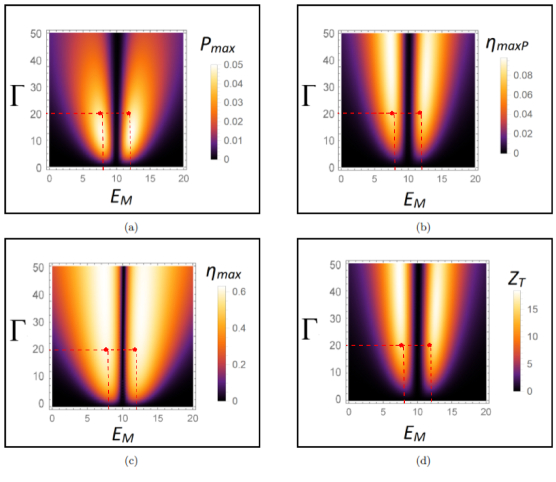
Figure 2: Thermoelectric parameters for the Majorana quantum heat engine (a) Maximum power in units of $P_{0}=(k_{B}^{2}T\Delta T)/h$, (b) Efficiency at maximum power $\eta_{maxP}$ in units of $\eta_{c}$, (c) maximum efficiency $\eta_{max}$ in units of $\eta_{c}$, (d) the figure of merit $Z_{T}/e$ where $e$ is the constant $1.6\times 10^{-19}$, vs. $\Gamma$ (in $\mu eV)$ and $E_{M}$ (in $\mu eV)$ for $E_{F}=10\mu eV$, $\phi=1.57\phi_{0}$, with $\phi_{0}=hc/e$. The optimal regimes are highlighted with red points.

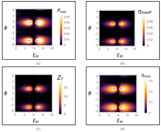
Figure 3: Thermoelectric parameters for the Majorana quantum heat engine (a) Maximum power in units of $P_{0}=(k_{B}^{2}T\Delta T)/h$, (b) Efficiency at maximum power $\eta_{maxP}$ in units of $\eta_{c}$, (c) the figure of merit $Z_{T}/e$ where $e$ is the constant $1.6\times 10^{-19}$, and (d) maximum efficiency $\eta_{max}$ in units of $\eta_{c}$, vs. $\phi$ (in units of $\phi_{0}$) and $E_{M}$ (in $\mu eV)$ for $E_{F}=10\mu eV$, $\Gamma=20\mu eV$. The optimal regimes are highlighted with red points.

$$\begin{split}e^{\uparrow}_{i5}=e^{ik_{e}l_{1}}e^{\dfrac{-i\phi l_{1}}{L}}e^{\uparrow}_{iL},e^{\uparrow}_{oL}=e^{ik_{e}l_{1}}e^{\dfrac{i\phi l_{1}}{L}}e^{\uparrow}_{o5},\\ h^{\uparrow}_{i5}=e^{ik_{h}l_{1}}e^{\dfrac{i\phi l_{1}}{L}}h^{\uparrow}_{iL},h^{\uparrow}_{oL}=e^{ik_{h}l_{1}}e^{\dfrac{-i\phi l_{1}}{L}}h^{\uparrow}_{o5},\end{split}$$ (23)

for the upper arm, right of STIM junction:

$$\begin{split}e^{\uparrow}_{o6}=e^{ik_{e}l_{2}}e^{\dfrac{i\phi l_{2}}{L}}e^{\uparrow}_{oR},e^{\uparrow}_{iR}=e^{ik_{e}l_{2}}e^{\dfrac{-i\phi l_{2}}{L}}e^{\uparrow}_{i6},\\ h^{\uparrow}_{o6}=e^{ik_{h}l_{2}}e^{\dfrac{-i\phi l_{2}}{L}}h^{\uparrow}_{oR},h^{\uparrow}_{iR}=e^{ik_{h}l_{2}}e^{\dfrac{i\phi l_{2}}{L}}h^{\uparrow}_{i6},\end{split}$$ (24)

For the lower arm of the ring:

$$\begin{split}e^{\uparrow}_{o3}=e^{ik_{e}l_{d}}e^{\dfrac{i\phi l_{d}}{L}}e^{\uparrow}_{o4},e^{\uparrow}_{i4}=e^{ik_{d}l_{d}}e^{\dfrac{-i\phi l_{d}}{L}}e^{\uparrow}_{i3},\\ h^{\uparrow}_{o3}=e^{ik_{h}l_{d}}e^{\dfrac{-i\phi l_{d}}{L}}h^{\uparrow}_{o4},h^{\uparrow}_{i4}=e^{ik_{h}l_{d}}e^{\dfrac{i\phi l_{d}}{L}}h^{\uparrow}_{i3},\end{split}$$ (25)

where $k_{e}=(E+E_{f})/\hbar v_{F}$, and $k_{h}=(E-E_{f})/\hbar v_{F}$. $\phi$ is the Aharonov-Bohm flux taken in units of the flux quantum $\phi_{0}=hc/e$. Similarly, One can find the phase acquired by the spin-down electrons and holes, which is the exact mirror image of spin-up electrons and holes. Using Eqs. (21-25), we can calculate the scattering amplitudes and the resulting transmission probability. We can then use the transmission probability $\mathcal{T}$ in Eq. (1) to calculate the thermoelectric parameters to quantify the performance of our quantum heat engine/refrigerator. In the next section, we study the thermoelectric performance of our setup and outline the parameters where the setup works as a heat engine and where it works as a refrigerator.

IV Thermoelectric Performance

IV.1 Majorana quantum heat engine

In Fig. 2, we plot the maximum power, the efficiency at maximum power, maximum efficiency, and the figure of merit when the system is acting as a heat engine vs. the coupling between the MBS and the ring ($\Gamma_{1}=\Gamma_{2}=\Gamma$), and the coupling strength between individual MBS ($E_{M}$) for $E_{F}=10\mu eV$ and $\phi=1.57\phi_{0}$. The maximum power output is plotted in Fig. 2 (a) vs. $\Gamma$ and $E_{M}$. At $\Gamma=0$, the STIM junction is wholly disconnected from the ring ($S_{MBS}=I$), and MBS are absent from the setup. For $\Gamma=0$, we see that the maximum power is zero [3] as particle-hole symmetry (PHS) is preserved in the setup [22, 23, 3]. As we increase $\Gamma$, the maximum power increases to a peak and slowly decays to zero. The maximum power is highest when $E_{M}$ is close to $E_{F}$ but not equal. If $E_{M}=E_{F}$, $P_{max}=0$, i.e., if the Fermi energy of the TI is equal to the energy of coupling between the MBS, the thermoelectric response vanishes as the Seebeck coefficient is zero at precisely $E_{F}=\pm E_{M}$ [3, 23]. The Seebeck coefficient changes sign at $E_{F}=\pm E_{M}$ as the dominant charge carrier changes from electrons to holes. As we move away from $E_{F}$ on both sides, the Seebeck coefficient increases in magnitude, thus improving the thermoelectric performance. On both sides of $E_{M}$, the maximum power increases to a peak and then decays to zero again. The rise and decay are rapid for lower $\ Gamma$, while the peaks are broadened for higher $\Gamma$. As we increase $\Gamma$, the STIM junction is strongly coupled to the ABI; thus, the breaking of PHS is more significant as we increase $\Gamma$ (Eq. (21)). This results in low electrical conductance and high Seebeck coefficients, leading to higher thermoelectric efficiency and lower maximum power (see Sec. V) [24, 8]. When $\Gamma$ is zero, PHS is preserved, and efficiency and maximum power are zero.

In Fig. 2 (b), we plot the efficiency at maximum power $\eta_{maxP}$ vs. $\Gamma$ and $E_{M}$. We see zero efficiencies at maximum power as expected for $\Gamma=0$ (MBS absent). As we increase $\Gamma$, $\eta_{maxP}$ increases to a finite value and remains finite for higher $\Gamma$. Similar to the maximum power, since the Seebeck coefficient changes sign at exactly $E_{M}=\pm E_{F}$, we see that $\eta_{maxP}$ is highest when $E_{M}$ is close to $E_{F}$ and zero when $E_{M}=E_{F}$. As we disappear from $E_{F}$, $\eta_{maxP}$ increases rapidly and slowly decays to zero. The efficiency at maximum power, the figure of merit (Fig. 2 (c)), and the maximum efficiency (Fig. 2 (d)) behave similarly to each other. From Fig. 2 (c), the maximum efficiency can reach up to $0.6\eta_{c}$. However, at maximum efficiency, the output power is minimal [8]. We look at Fig. 2 (b), the efficiency at maximum power; we see that for $E_{M}=8\mu eV$, and $\Gamma=20\mu eV$, we have $P_{max}=0.05P_{0}$ with $\eta_{maxP}=0.08\eta_{c}$, with $P_{0}=(k_{B}^{2}T\Delta T)/h$. From Fig. 3, we see that for $\phi=1.57\phi_{0}$, and $E_{M}=8\mu eV$, we find $P_{max}=0.05P_{0}$, and $\eta_{maxP}=0.03\eta_{c}$. Thus, the optimal performance is for $\phi=1.57\phi_{0}$, $E_{M}=8\mu eV$, and $\Gamma=20\mu eV$ giving $P_{max}=0.05P_{0}$ and $\eta_{maxP}=0.08\eta_{c}$. The optimal performance can also be reached at $\phi=1.57\phi_{0}$ and $E_{M}=12\mu eV$, with $\Gamma=20\mu eV$.

In Fig. 3, we plot the same parameters vs. the Aharonov-Bohm flux $\phi$, and $E_{M}$ for $E_{F}=10\mu eV$, and $\Gamma=20\mu eV$. The maximum power, efficiency at maximum power, the figure of merit, and maximum efficiency behave similarly when plotted against $\phi$ and $E_{M}$. The parameters are periodic with respect to $\phi$ with a $2\pi$ period. For finite $E_{M}$, i.e., coupled MBS, the thermoelectric parameters are asymmetric with respect to $\phi$. The asymmetry in the thermoelectric parameters results from the breaking of time reversal symmetry and particle-hole symmetry by the MBS and the Aharonov-Bohm flux. The reasons for this asymmetry are detailed in Sec. V. Similar to Fig. 2, we see that the performance is best when $E_{M}$ is close to $E_{F}$, and zero when $E_{M}=E_{F}$. As we go away from $E_{F}$, the parameters rapidly increase to a peak and then decay to zero. We see that the thermoelectric parameters are periodic with respect to $\phi$ with a period of $2*\pi$. Thus, the optimal performance can also be reached for $\phi=-4.71\phi_{0}$ while keeping $E_{M}=8\mu eV$ or $E_{M}=12\mu eV$ with $\Gamma=20\mu eV$.

From Figs. 2-3, we can study the behavior of the thermoelectric parameters with respect to the presence and nature of MBS in the system. Fig. 2 shows that the thermoelectric parameters are zero when MBS is absent, i.e., $\Gamma=0$. When MBS are present in the system, we can use the symmetry of the thermoelectric parameters with respect to the Aharonov-Bohm flux $\phi$ to distinguish their nature. From Fig. 3, we can see that for $E_{M}=0$, or individual MBS, the thermoelectric parameters are symmetric with respect to $\phi$. For coupled MBS ($E_{M}\neq 0$), the parameters behave asymmetrically with respect to $\phi$. Thus, the symmetry of the thermoelectric parameters can be used as a probe to detect the presence and nature of MBS in the setup. The reasons for this behavior are elaborated further in Sec. V.

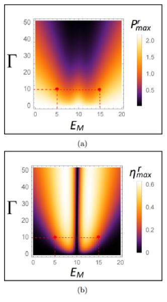
Figure 4: (a) Maximum cooling power $P^{r}_{max}$ in units of $P_{0}$, and (b) maximum COP $\eta^{r}_{max}$ in units of $\eta^{r}_{c}$, vs $\Gamma$ (in $\mu eV)$ and $E_{M}$ (in $\mu eV)$ for $E_{F}=10\mu eV$, $\phi=\phi_{0}$. The optimal regimes are highlighted with red points.

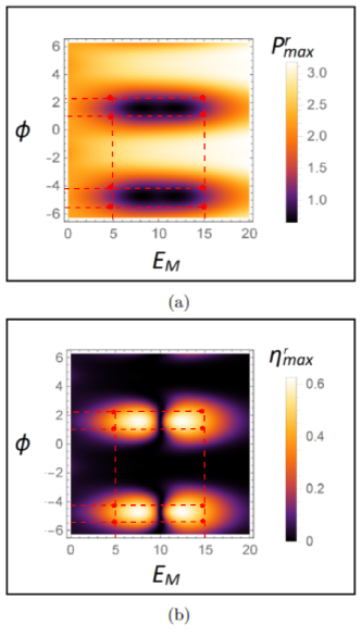
Figure 5: (a) Maximum cooling power $P^{r}_{max}$ in units of $P_{0}$, and (b) maximum COP $\eta^{r}_{max}$ in units of $\eta^{r}_{c}$, vs $\phi$ (in units of $\phi_{0}$) and $E_{M}$ (in $\mu eV)$ for $E_{F}=10\mu eV$, $\Gamma=10\mu eV$. The optimal regimes are highlighted with red points.

IV.2 Majorana quantum refrigerator

In this subsection, we look at the setup’s performance when acting as a quantum refrigerator. In Fig 4 (a), we plot the cooling power at maximum efficiency vs. $\Gamma$ and $E_{M}$, with $E_{F}=10\mu eV$ and $\phi=1.57\phi_{0}$. The cooling power is maximum at very low $\Gamma$ and decays to zero as we increase $\Gamma$. In Fig. 4 (b), we plot the maximum coefficient of performance vs. $\Gamma$ and $E_{M}$ for the same $E_{F}$ and $\phi$. Similar to Fig. 2 (c), we see that for $\Gamma=0$, i.e., when MBS are absent from the setup, the maximum COP is zero as particle-hole symmetry is preserved in the absence of MBS. We also see that for $E_{M}=E_{F}$, the maximum COP is zero. As we move away from $E_{F}$ in both directions, the maximum COP rapidly increases to a peak and then slowly decays. For higher $\Gamma$, since the electrical conductance is small and the Seebeck coefficient is high, we see a large COP and small cooling power. For lower $\Gamma$, the STIM junction is weakly coupled, and the electrical conductance is large. This results in lower COP but higher cooling power [24, 8] (see Sec. V). Comparing Fig. 4 (a) with Fig. 4 (b), we see that the maximum COP and the cooling power are complementary to each other, i.e., as COP increases, cooling power decreases and vice-versa.

We plot the cooling power in Fig. 5 (a) and maximum COP in Fig. 5 (b) vs. $\phi$ and $E_{M}$ with $E_{F}=10\mu eV$, and $\Gamma=10\mu eV$. Similar to the heat engine parameters, the cooling power, and the maximum COP are periodic with respect to $\phi$ with a period of $2\pi$. From Fig. 5 (a), we see that the cooling power is not necessarily high or low for $E_{M}=E_{F}$. Similar to Fig. 4, we see that the cooling power and maximum COP are complementary. In regions with high COP, we see the lowest cooling power. By inspecting the figures, we can find the optimal balance of COP and cooling power with respect to $\phi$. From Figs. 4-5, we see that the optimal performance for setup as a quantum refrigerator is for $E_{F}=10\mu eV$, $\Gamma=10\mu eV$, with the optimal points $(E_{M},\phi)$ given by $(5\mu eV,\phi_{0})$, $(5\mu eV,2.14\phi_{0})$, $(5\mu eV,-4.14\phi_{0})$, $(5\mu eV,-5.28\phi_{0})$, $(15\mu eV,\phi_{0})$, $(15\mu eV,2.14\phi_{0})$, $(15\mu eV,-4.14\phi_{0})$, $(15\mu eV,-5.28\phi_{0})$, we get $P^{r}_{max}=1.8P_{0}$ with $\eta^{r}_{max}=0.45\eta^{r}_{c}$. We cannot plot COP at maximum cooling power, as in a quantum refrigerator, there is no bound on the maximum power [8]. Thus we only plot the maximum COP and the cooling power at maximum COP.
Like the heat engine parameters, when MBS are absent ($\Gamma=0$), PHS is unbroken, and the maximum COP is zero, but the cooling power remains constant. Since the maximum COP in the absence of MBS is zero, we cannot use the setup as a quantum refrigerator without MBS. In the presence of MBS, once again, we see that the cooling power and COP are symmetric with respect to $\phi$ in the presence of individual MBS ($E_{M}=0$) and asymmetric with respect to $\phi$ when coupled MBS are present ($E_{M}\neq 0$). Thus, the symmetry in cooling power and COP with respect to $\phi$ can also be used to probe the existence and nature of MBS.

Comparing Figs. 2-3 with Figs. 4-5, we see that the regions where the setup functions as a quantum heat engine are complementary to the regions where the setup functions as a quantum refrigerator, i.e., in the regions where the performance is high as a quantum heat engine, the performance as a quantum refrigerator is poor and vice-versa. Thus, the setup cannot simultaneously work as a quantum heat engine and a quantum refrigerator. The setup works as an optimal quantum heat engine or an optimal quantum refrigerator for any set of parameters.

V Analysis

In Table I, we compare the performance of the Majorana heat engine with other contemporary nanoscale quantum heat engines. We show that our proposed setup can outperform some quantum heat engines, like the cavity heat engine proposed in [9]. We also show that our proposed setup can have higher efficiencies than other quantum heat engines like the three-terminal quantum spin Hall heat engine proposed in [10] with lower output power. The maximum power $P_{max}$ can reach up to $0.05P_{0}$ for lower efficiency.
In Table II, we compare the performance of the Majorana refrigerator with other nanoscale quantum refrigerators. We see that our proposed setup outperforms the quantum refrigerators considered here. For the optimal parameters, the cooling power at maximum COP $P^{r}_{max}=1.8P_{0}$ and the corresponding maximum COP is given by $\eta^{r}_{max}=0.45\eta^{r}_{c}$. Fig. 4 shows that the cooling power can reach up to $3.0P_{max}$ with very low COP. Conversely, from Fig. 5, we see that for very little cooling power, the maximum COP can go up to $0.6\eta^{r}_{c}$.

Quantum heat Engine	Maximum power (in units of $P_{0}$)	Efficiency at Maximum power (in units of $\eta_{c}$)
Quantum Hall heat engine (two-terminal) [10]	0.14	0.10
Quantum Hall heat engine (three-terminal) [10]	0.14	0.042
Chaotic Cavity [9]	0.0066	0.01
Strained graphene Quantum Hall heat engine [11]	0.268	0.1
Majorana quantum heat engine (This paper)	0.05	0.08

Table 1: Comparing the MBS heat engine to other contemporary heat engines.

Quantum Refrigerator	Maximum cooling power (in units of $P_{0}$)	Maximum coefficient of performance (in units of $\eta^{r}_{c})$
Strained graphene refrigerator [13]	2.0	0.4
Three-terminal quantum dot refrigerator [15]	0.87	0.4
Magnon-driven quantum dot refrigerator [14]	0.8	0.2
Majorana quantum refrigerator (This paper)	1.8	0.45

Table 2: Comparing the MBS refrigerator to other contemporary refrigerators.

From Eq. (9), we see that in the case of a quantum heat engine, the condition for a high $P_{max}$, within the linear response regime, is $L_{cT}>>L_{cV}$ [24, 11], i.e., the Seebeck coefficient must be greater than the electrical conductance so that the thermoelectric response is high. The finite Seebeck coefficient arises only due to the Majorana bound states and the flux in our setup. The Seebeck coefficient is not high compared to the electrical conductance. Thus, we see a minimal maximum power when the setup acts as a quantum heat engine. On the other hand, in the case of a quantum refrigerator, for the cooling power $P_{max}^{r}$ to be high, the electrical conductance $L_{cV}$ and the thermal response to the temperature gradient $L_{qT}$ must be high. At the same time, the Seebeck coefficient must be low (Eq. (9)) [24, 13]. It explains why the setup acts as a highly powerful quantum refrigerator but fails to act as an equally capable quantum heat engine. We also see that the performance is best when $E_{F}$ is close to $E_{M}$ but not equal. When $E_{M}=E_{F}$, there is a dip in the conductance, and the Seebeck coefficient vanishes because the dominant charge carriers change from electrons to holes; this results in zero efficiency and coefficient of performance. As we move away from $E_{F}$ on both sides, the conductance changes rapidly, and the Seebeck coefficient is very high, leading to high efficiency and coefficient of performance. Similar behavior of the thermoelectric figure of merit with respect to $E_{F}$ and $E_{M}$ has been reported in [3], albeit with a massive reduction in magnitude. The increased thermoelectric efficiency of our setup is attributed to the presence of an Aharonov-Bohm flux, in addition to the MBS, that is not present in previous works.

Another application of our proposed setup is distinguishing the existence and nature of MBS in the setup. From Figs. 2 and 4, we can see that when MBS is absent, i.e., $\Gamma=0$, the thermoelectric parameters maximum power, maximum efficiency, the figure of merit, efficiency at maximum power, and maximum COP vanish, and the cooling power remains constant. The reason for vanishing the efficiencies is the preservation of time-reversal symmetry (TRS) and particle-hole symmetry (PHS) in the system in the absence of MBS. When MBS are present, particle-hole symmetry is broken, and we get finite thermoelectric parameters. MBS can be individual ($E_{M}=0$) or coupled ($E_{M}\neq 0$). We use the symmetry with respect to the Aharonov-Bohm flux $\phi$ (see Figs. 3, 5) to distinguish between individual and coupled MBS. For individual MBS, we see that the thermoelectric parameters are symmetric with respect to $\phi$. For coupled MBS, the thermoelectric parameters are asymmetric with respect to $\phi$. The main reason for breaking the symmetry in the thermoelectric parameters is the breakdown of TRS due to the Aharonov-Bohm flux when MBS are coupled. When MBS are coupled ($E_{M}\neq 0$), the symmetry in the S-matrix given in Eq. (21) is broken as $y(E)\neq y(-E)$. It makes the S-matrix in Eq. (21) asymmetric, which results in asymmetric transport with respect to the reversal of Aharonov-Bohm flux due to the breakdown of TRS. If $E_{M}=0$, only PHS is broken, and we get finite but symmetric thermoelectric parameters. This distinct behavior of the thermoelectric parameters for the absence of MBS, the presence of individual MBS, and the presence of coupled MBS can be used to detect the existence and nature of MBS in the setup [23] via the maximum power and efficiencies of either the Majorana quantum heat engine or the Majorana quantum refrigerator.

VI Conclusion

In this paper, we have proposed a setup that can act as a viable Majorana quantum heat engine and Majorana quantum refrigerator in separate parameter regimes due to the presence of Majorana-bound states. We have shown that the presence of Majorana bound states significantly increases the setup’s performance, both as a quantum heat engine and as a quantum refrigerator. We have outlined the effect of various parameters, such as the coupling strength of the STIM junction to the ring $\Gamma$, the strength of coupling between individual MBS ${}^{\prime}E_{M}^{\prime}$, and the Aharonov-Bohm flux $\phi$ piercing the ring. We show that the maximum efficiency and maximum COP of the system vanish in the absence of MBS. Thus, we cannot use the setup as a quantum heat engine or quantum refrigerator without MBS. In the presence of MBS, we find that for the parameters $(E_{M},\phi)=$ $(8\mu eV,1.57\phi_{0})$, $(8\mu eV,-4.71\phi_{0})$, $(12\mu eV,1.57\phi_{0})$ or $(12\mu eV,-4.71\phi_{0})$, with $\Gamma=20\mu eV$, the performance as a heat engine is best with $P_{max}=0.05P_{0}$, and $\eta_{maxP}=0.08\eta_{c}$. For the parameters $\Gamma=10\mu eV$, with $(E_{M},\phi)$ = $(5\mu eV,\phi_{0})$, $(5\mu eV,2.14\phi_{0})$, $(5\mu eV,-4.14\phi_{0})$, $(5\mu eV,-5.28\phi_{0})$, $(15\mu eV,\phi_{0})$, $(15\mu eV,2.14\phi_{0})$, $(15\mu eV,-4.14\phi_{0})$, $(15\mu eV,-5.28\phi_{0}),$ we see that the setup works as an optimal refrigerator with $P^{r}_{max}=1.8P_{0}$, and $\eta^{r}_{max}=0.45\eta_{c}$, which is higher than some of the best contemporary nanoscale steady-state refrigerators. Since the efficiencies vanish in the absence of MBS, we have shown that it is the presence of MBS that makes it possible for the setup to work as a viable quantum heat engine and refrigerator.
When MBS are absent, the thermoelectric parameters maximum power, maximum efficiency, the figure of merit, efficiency at maximum power, and maximum COP vanish while the cooling power remains constant. When uncoupled MBS are present in the system, the thermoelectric parameters are symmetric with respect to $\phi$. When MBS are coupled, the thermoelectric parameters are asymmetric with respect to $\phi$. This behavior can be used to detect the presence and nature of MBS.

References

- Sarma et al. [2006] S. D. Sarma, M. Freedman, and C. Nayak, Topological quantum computation, Physics Today 59, 32 (2006).
- Kitaev [2006] A. Kitaev, Anyons in an exactly solved model and beyond, Annals of Physics 321, 2 (2006).
- Ramos-Andrade et al. [2016] J. P. Ramos-Andrade, O. Ávalos-Ovando, P. A. Orellana, and S. E. Ulloa, Thermoelectric transport through majorana bound states and violation of wiedemann-franz law, Phys. Rev. B 94, 155436 (2016).
- Samuelsson et al. [2017] P. Samuelsson, S. Kheradsoud, and B. Sothmann, Optimal quantum interference thermoelectric heat engine with edge states, Phys. Rev. Lett. 118, 256801 (2017).
- Hofer and Sothmann [2015a] P. P. Hofer and B. Sothmann, Quantum heat engines based on electronic mach-zehnder interferometers, Phys. Rev. B 91, 195406 (2015a).
- Muttalib and Hershfield [2015] K. A. Muttalib and S. Hershfield, Nonlinear thermoelectricity in disordered nanowires, Phys. Rev. Applied 3, 054003 (2015).
- Beenakker and Staring [1992] C. W. J. Beenakker and A. A. M. Staring, Theory of the thermopower of a quantum dot, Phys. Rev. B 46, 9667 (1992).
- Whitney [2014] R. S. Whitney, Most efficient quantum thermoelectric at finite power output, Phys. Rev. Lett. 112, 130601 (2014).
- Sothmann et al. [2012] B. Sothmann, R. Sánchez, A. N. Jordan, and M. Büttiker, Rectification of thermal fluctuations in a chaotic cavity heat engine, Phys. Rev. B 85, 205301 (2012).
- Hofer and Sothmann [2015b] P. P. Hofer and B. Sothmann, Quantum heat engines based on electronic mach-zehnder interferometers, Phys. Rev. B 91, 195406 (2015b).
- Mani and Benjamin [2017] A. Mani and C. Benjamin, Strained-graphene-based highly efficient quantum heat engine operating at maximum power, Phys. Rev. E 96, 032118 (2017).
- Benenti et al. [2017] G. Benenti, G. Casati, K. Saito, and R. Whitney, Fundamental aspects of steady-state conversion of heat to work at the nanoscale, Physics Reports (2017).
- Mani and Benjamin [2019] A. Mani and C. Benjamin, Optimal quantum refrigeration in strained graphene, The Journal of Physical Chemistry C 123, 22858 (2019).
- Wang et al. [2015] Y. Wang, C. Huang, and J. Chen, Magnon-driven quantum dot refrigerators, Physics Letters A 379 (2015).
- Zhang et al. [2015] Y. Zhang, G. Lin, and J. Chen, Three-terminal quantum-dot refrigerators, Phys. Rev. E 91, 052118 (2015).
- Benenti et al. [2011] G. Benenti, K. Saito, and G. Casati, Thermodynamic bounds on efficiency for systems with broken time-reversal symmetry, Phys. Rev. Lett. 106, 230602 (2011).
- Buttiker et al. [1983] M. Buttiker, Y. Imry, and R. Landauer, Josephson behavior in small normal one-dimensional rings, Physics Letters A 96, 365 (1983).
- Fu and Kane [2008] L. Fu and C. L. Kane, Superconducting proximity effect and majorana fermions at the surface of a topological insulator, Phys. Rev. Lett. 100, 096407 (2008).
- Fu and Kane [2009] L. Fu and C. L. Kane, Josephson current and noise at a superconductor/quantum-spin-hall-insulator/superconductor junction, Phys. Rev. B 79, 161408 (2009).
- Nilsson et al. [2008] J. Nilsson, A. R. Akhmerov, and C. W. J. Beenakker, Splitting of a cooper pair by a pair of majorana bound states, Phys. Rev. Lett. 101, 120403 (2008).
- Benjamin and Pachos [2010] C. Benjamin and J. K. Pachos, Detecting majorana bound states, Phys. Rev. B 81, 085101 (2010).
- Leijnse [2014] M. Leijnse, Thermoelectric signatures of a majorana bound state coupled to a quantum dot, New Journal of Physics 16, 015029 (2014).
- Das and Benjamin [2022] R. Das and C. Benjamin, Probing majorana bound states via thermoelectric transport, arXiv:2207.01515 (2022).
- Mani and Benjamin [2018] A. Mani and C. Benjamin, Helical thermoelectrics and refrigeration, Phys. Rev. E 97, 022114 (2018).