Recursions and characteristic polynomials of the Rows of the Circuit Array

Abstract.

The 2022 Fibonacci Conference held in Sarajevo introduced the Circuit Array, a two-dimensional array associated with the resistance labels of electrical circuits whose underlying graph when embedded in the Cartesian plane has the form of a triangular n-grid. The presentation used row reduction, a computational method alternative to the traditional method using the Laplacian. The presentation explored reconsidering the Circuit Array in terms of polynomials instead of numbers as a means to facilitate finding patterns. The present paper shows the fruitfulness of this approach. The main result of the current paper states that the characteristic polynomials corresponding to the recursions of single or multi-variable polynomial formulations of the Circuit Array exclusively have powers of 9 as roots. The proof methodology uses the approach of annihilators. Several initial cases and one major sub-case are proven.

KEYWORDS: effective resistance, resistance distance, triangular grids, circuit simplification, circuit array, annihilator, polynomial recursions

1. Introduction

1.1. Goals

In prior work [7], the authors introduced the Circuit Array, a two-dimensional array associated with the resistance labels of electrical circuits whose underlying graphs when embedded in the Cartesian plane have the form of a triangular n-grid. The Circuit Array is constructed by applying a sequence of equivalent network transformations to an initial electrical circuit and selecting specified edge-label resistances. The prior work presented several approaches to studying patterns in the sequences of the rows of the Circuit Array. The main result of the current paper states that the roots of the characteristic polynomial (annihilator) of row $i,i\geq 0,$ of the Circuit Array, when it is re-formulated in terms of single or multi-variable polynomials, exclusively has roots which are powers of 9.

The proof methodology uses the method of annihilators. This method is an old, powerful, and easily applied technique originally introduced by Boole [4]. Several authors have recently begun using them again when studying recursions [5, 11].

1.2. History of Effective Resistance

We state at the outset that the focus of this paper is about recursions, characteristic polynomials, and annihilators satisfied by certain sequences. More specifically, familiarity with the underlying electrical circuit theory is not needed to fully appreciate this paper. It suffices to know the four functions presented in Section 4 which will be fully illustrated with examples in Section 5. Knowledge about the electrical interpretation of these functions, while interesting historically, would not increase understanding.

To develop this point, that knowledge of electrical circuit theory is not needed to understand this paper, we briefly review several approaches to (exact) computations of effective resistance in a graph. First, we recall that effective resistance, also termed in the literature resistance distance, is a graph metric whose definition was motivated by the consideration of a graph as an electrical circuit. A formal definition of this metric can be found in [7], but it is essentially computed by first assuming the graph is an electric circuit with each edge replaced by an one-ohm resistor. The effective resistance is then calculated by considering the potential difference between two nodes in a graph when one unit of current is introduced. There are many ways to calculate this quantity (exactly) and we review several historically relevant techniques.

• The initial approach to computing resistances was to use the Kirchoff laws which at least theoretically allowed solving any electrical circuit.

• However, for a circuit whose underlying graph is embeddable in the Cartesian plane, all computations and simplifications of this circuit can be made with four well-known circuit transformation functions: parallel, series, $\Delta-Y,$ and $Y-\Delta.$ These four circuit transformation functions reduce the complexity of the underlying graph while leaving the effective resistance between two vertices of interest the same.

• For circuits derived from small graphs or graphs with special structures, the computational graph Laplacian is frequently used to compute resistances between two points in a circuit [1, 2].

• For triangular $n$-grids, [2, 11] exploit the idea of reducing the number of rows in the underlying, initial, triangular $n$-grid one row at a time. This can be accomplished by the four electrical circuit functions. [2] used this idea to accomplish proofs while [11] was the first to show its computational advantages in discovering patterns.

• To make the computations of resistance labels arising from reductions, [7, 8] showed that only four functions, each of which takes up to nine arguments, need be considered. These four functions calculate resistance labels for a i) left-boundary, ii) left-interior, iii) right, and iv) base edge of a given triangle in a triangular $n$-grid reduced once.

• This paper, while still using only four functions, shows, in certain cases, how to reduce the maximum number of arguments of these functions from 9 to 4. This greatly simplifies computations, facilitates discovery of patterns, and is a key tool in proofs.

• There is also a rich theory for calculating effective resistances using probabilitic and numerical methods which however will not be used in this paper, [6].

It follows, as stated at the beginning of this section, that to understand the results of this paper, it suffices to know these four functions and how they are used on labeled graphs.

1.3. Outline.

An outline of this paper is the following.

• Section 2 gives necessary terminology and notational conventions.

• Section 3 formulates a 5-dimensional representation of the numerical values of edge labels in a collection of triangular-grids resulting from reducing an original $n$-grid one row at a time. A 3-dimensional representation of this 5-dimensional space is also introduced. These representations help account for the ad-hoc appearance of certain sequences with recursive patterns that are studied throughout the paper. The section then presents the numerical Circuit Array as well as two polynomial Circuit Arrays. The row sequences of these arrays are the object of study of this paper.

• Section 4 presents the four circuit transformations needed to understand this paper.

• Section 5 presents a detailed example which integrates all computational techniques used including use of theorems. An understanding of this example should suffice for purposes of reading this paper.

• Section 6 completely but briefly reviews the theory of annihilators with adequate references and illustrative examples.

• Section 7 states and proves the main theorem for the one-variable Circuit Array, while Section 8 presents corresponding results for the multi-variable circuit array.

• Section 9 concludes with an interesting conjecture about the polynomial form of the one-variable members of the one-variable Circuit Array.

2. Background

In this section we will review important terminology and concepts. The material in this section is taken almost verbatim from [7, 8, 11]; therefore, attribution to the original and subsequent sources are omitted below except for a few important concepts.

2.1. The $n$-grid.

Definition 2.1.

A $n$-triangular-grid (usually abbreviated as an $n$-grid) is any graph that is (graph-) isomorphic to the graph, whose vertices are all integer pairs $(x,y)=(2r+s,s)$ in the Cartesian plane, with $r$ and $s$ integer parameters satisfying $0\leq r\leq n,0\leq s\leq n-r;$ and whose edges consist of any two vertices $(x,y)$ and $(x^{\prime},y^{\prime})$ with either i) $x^{\prime}-x=1,y^{\prime}-y=1,$ ii) $x^{\prime}-x=2,y^{\prime}-y=0,$ or iii) $x^{\prime}-x=1,y^{\prime}-y=-1.$

Figure 1. A 3-grid embedded in the Cartesian Plane (Panel A) with row and diagonal coordinates (Panel B).

Figure 1 illustrates this definition along with various notational conventions which are thoroughly explaineed below.

Note, that throughout this paper the edge labels of a graph correspond to actual resistance values.

2.2. The $\Delta$ and $Y$ Functions.

The $\Delta-Y$ and $Y-\Delta$ functions defined from circuit transformations are given by (2.1).

$$\Delta(x,y,z)=\frac{xy}{x+y+z};\qquad Y(a,b,c)=\frac{ab+bc+ca}{a}.$$ (2.1)

Conventions on the order of the arguments are illustrated in Figure 2.

Figure 2. Definition and assumed orientation of the $\Delta$ (that is $\Delta$–Y) and $Y$ (that is the Y–$\Delta$) functions of electrical resistance. $P,Q,R$ are vertex labels; $L,R,B$ are edge labels standing for left, right, and bottom edge. We use e.g. $L$ to refer both to the left edge and to the label of the left edge; meaning should be clear from context.

2.3. Weighted graphs perceived as circuits.

The effective resistance metric considers weighted graphs as circuits where each edge in the graph corresponds to a resistor whose resistance is the reciprocal of the edge weight. This important concept is illustrated in Figure 3 using the very simple series transformation from electrical circuit theory.

In Figure 3, we note that in going from the parent (top) graph to the child (bottom) graph, the following has occurred:

• One node and one edge have been removed from the parent graph to yield the child graph.

• The well known series transformation (see, e.g.,  [2]) equates the numerical edge label of the child graph to a functional value of the edge labels of the parent graph.

• This transformation is equivalent; the effective resistance between nodes and A and C are the same in the parent and child graph.

Figure 3. Illustration of the series transformations. More detail is provided in the narrative.

2.4. The Reduction Algorithm

As mentioned in Section 1.2, row reduction is an algorithm that takes an $n$-grid and creates an $n-1$ grid. The algorithm may be formulated using series, $\Delta$–Y, and Y–$\Delta$ transformations. Given an $n$-grid with labeled edges, the row-reduction of this labeled $n$-grid (to a labeled $n-1$ grid) refers to the sequential performance of the following steps (with illustrations of the steps provided by Figure 4).

• Step 1 - Panel A: Start with an all-one 3-grid, that is, a 3-grid all of whose edges are labeled 1.

• Step 2 - Panel B: Apply a $\Delta-Y$ transformation to each upright triangle (a 3-loop) resulting in a grid of 3 rows of 3-outstars, as shown.

• Step 3 - Panel C: Discard the corner tails, edges with a vertex of degree one. This does not affect the resistance labels of edges in the reduced two grid in panel E. (However, these corner tails are useful for computing certain effective resistances as shown in [3, 9]).

• Step 4 - Panel D: Perform series transformations on all consecutive pairs of boundary edges (i.e., the dashed edges in panel C).

• Step 5 - Panel E: Apply $Y-\Delta$ transformations to all remaining 3-outstars, transforming them into 3-loops.

Figure 4. Illustration of the reduction algorithm, on a 3-grid. The panel labels correspond to the five steps indicated in the narrative.

2.5. Notational Conventions and definitions.

In this paper we will utilize the notation $T_{r,d,e}$ to refer to the edge label of edge $e,e\in\{L,R,B\}$ (standing, respectively, for the left, right, and base edges of a triangle in the upright oriented position), of the triangle in row $r$ diagonal $d.$ Similarly, $T_{r,d}$ will refer to the entire triangle in row $r$ diagonal $d.$ On occasion we may substitute $1,2,3$ for $L,R,B$ respectively.

Definition 2.2 (The all-one $n$-grid).

The all-one $n$-grid refers to an $n$-grid all of whose resistance values are uniformly 1.

The notations $T^{c}_{r,d,e}$ and $T^{c}_{r,d}$ refer respectively to edges and triangles in an initial all-one $n$ grid reduced $c$ times.

2.6. The Upper Left Half

Definition 2.3 (The Upper Left Half).

Given an integer $m$ the upper left half of the $m$ grid, is the set of triangles

$$S=\left\{T_{r,d}:1\leq d\leq\left\lfloor\frac{m+2}{3}\right\rfloor,2d-1\leq r\leq\left\lfloor\frac{m+d}{2}\right\rfloor\right\}.$$ (2.2)

Hendel, [11, Corollary 9.6] observes that because of the symmetries of the $m$-grid, knowledge of the edge labels of the triangles in the upper half suffices to determine the edge labels of all its triangles.

2.7. The Uniform Center.

In [8] the authors proved that under mild conditions ($n\geq 4s$) the central portion of the $n$ grid reduced $s$ times has a certain uniformity, that is, the triangles in this central region are uniformly labeled. More specifically, they proved the following result.

Theorem 2.4 (Uniform Center).

Given an initial all–one $n$–grid we can say the following.

1. For

   $$n\geq 4s,1\leq d\leq s,s+d\leq r_{1},r_{2}\leq n-2s,\text{and }e\in\ \{1,2,3\}$$

   we have

   $$T^{s}_{r_{1},d,e}=T^{s}_{r_{2},d,e}.$$ (2.3)

   In other words, in this region of the grid the triangle labels are uniform.

2. With the same constraints on $s,d,$ as in Part (i), and with $2s-1\leq r\leq n-2s$ we have

   $$T^{s}_{r,s,B}=T^{s}_{r,s,R}.$$ (2.4)

3. For

   $$n\geq 4s,2s+1\leq r\leq n-s,s+1\leq d\leq n-s,e\in\{L,R,B\},$$

   $$T^{s}_{r,d,e}=1.$$ (2.5)

   Additionally, we have

   $$T_{2s-1,s,e}^{s}=1,\qquad e\in\{R,B\}.$$

Comment 2.5.

As pointed out in [8, 11], one can think of the $m$ grid as composed of concentric layers of triangular rims. A consequence of the theorem is that the triangular rim (i.e. sub-grid) whose corners are $T^{s}_{2s-1,s},T^{s}_{n+1-2s,2},T^{s}_{n+1-2s,n+2-3s}$ has uniform labels on its boundaries and is uniformly one on its interior. However, this will not be needed in the sequel.

3. The Five Dimensional Hyperspace

3.1. The 5 Dimensional Hyperspace

The Circuit Array presented in Section 3.4 arises from a highly non-intuitive selection of edge-label resistances which just happen to have remarkable patterns. Because of this, the reader is left with the impression that perhaps some motivating perspective has been omitted. Unfortunately, that is not true. The authors took two years to discover these patterns and even then it was stumbled onto by accident. The purpose of this section is to clarify this complexity of patterns. The complexity arises from the reduction algorithm (Section 2.4); this algorithm creates a five dimensional hyperspace which allows emergence of a richness and plethora of patterns.

The five dimensions are:

• $n,$ the number of rows in an initial all-one $n$-grid

• $c,$ the number of single reductions performed on the initial $n$-grid

• The row, diagonal, and face (triangular edge) coordinates, ($r,d,e$), of the triangle in row $r$ diagonal $d$ in the $n-c$ grid arising from $c$ reductions of the initial all one $n$-grid.

3.2. A 3 Dimensional Visualization

For a given initial $n,$ We can conveniently visualize this 5 dimensional hyperspace, by creating a tetrahedron in $\mathbb{R}^{3}.$ The bottom triangle is placed on the plane $z=0$ and consists of an all-one $n$-grid, (Definition 2.1), whose base coincides with the $x$-axis. Using the reduction algorithm (Section 2.4) we reduce this labeled $n$-grid to an $n-1$ grid. This $n-1$ grid is placed in the plane $z=1$ with its bottom row on the line $y=1.$ Such a placement allows the top-corner triangles (that is, row 1, diagonal 1) of the $n$-grid and $n-1$-grid to lie on top of each other. We can then continue, reducing one row at a time and placing an $n-c$-grid (arising from $c$ reductions of the original all-one $n$-grid) in the plane $z=c$ with its base row on the line $y=c.$ The resulting tetrahedron contains all labels in all reductions of the original all one $n$-grid. See Figure 5 for an illustration.

3.3. Two Examples of slices of the 5 Dimensional Hyperspace

Two examples, previously studied, of “slices” of this 5-dimensional space with interesting patterns are the following:

• Hendel [11] studied the case where $n$ is going to infinity, $n-c$ is bounded, and $r,d,e$ are arbitrary. In terms of the three dimensional representation, this would correspond to the upper corner of the Tetrahedron when $n$ is arbitrarily large. [11] presents computational evidence that resistance labels are simple fractional multiples of $\frac{1}{e}.$ While supportive results are proven, and despite the simplicity of the statement of the conjecture, a proof eludes us at present.

• For $c=1,2,3,\dotsc$ the authors, [7], looked at the sequence,

  $$T^{c}_{2c-1,c,L}=\left\{\frac{2}{3},\frac{26}{27},\frac{242}{243},\dotsc\right\},=1-\frac{1}{3\cdot 9^{c}}.$$

  The point made at the beginning of this section can be appreciated by using the three dimensional presentation. We obtain this sequence by slicing the tetrahedron through the line given by the coordinates $(z,2z-1,z),z=1,2,3,\dotsc.$ Thus while the recursive pattern describing this sequence is clear and simply formulated the method of slicing the tetrahedron is highly non-intuitive; that is, one would not have thought of looking at the stated sequence; moreover, it is surprising that such a slice should give rise to such a simply stated pattern.

3.4. The Circuit Array.

The sequence just studied (Section 3.3) is the first row of the Circuit Array which we now fully define ([7]). The entry in the $i$-th row, $j$-th column, $0\leq i\leq 2(j-1),j\geq 1,$ of the Circuit Array, $C_{i,j}$, is given by

$$C_{i,j}=T^{j}_{2j-1,j-\lfloor\frac{i+1}{2}\rfloor,LR}$$

where $LR$ refers to the left edge (right edge) if $i$ is even (respectively odd).

Example 3.1.

If $i=0,$ then $C_{i,j}=C_{0,j}$ and we recover the sequence studied in Section 3.3

Tables 1 and 2 present the Circuit Array. Table 2 gives the numerical values of the Circuit Array; Table 1 gives the addresses of these labels in the 3-dimensional representation (that is, the number of reductions, the row, and diagonal of the underlying triangle).

The details of computation of values in this array are presented in [7]. The numerical entries in Table 2 can be computed using the reduction algorithm (Algorithm 2.4). In Section 4.5, we present two illustrative computational examples.

Table 1. First few rows and columns of the symbolic entries (i.e. addresses) of the numerical Circuit Array.

	$1$	$2$	$3$	$4$	$5$	$6$	$7$	$\dotsc$
$0$	$T_{1,1,L}^{1}$	$T_{3,2,L}^{2}$	$T_{5,3,L}^{3}$	$T_{7,4,L}^{4}$	$T_{9,5,L}^{5}$	$T_{11,6,L}^{6}$	$T_{13,7,L}^{7}$	$\dotsc$
$1$		$T_{3,1,R}^{2}$	$T_{5,2,R}^{3}$	$T_{7,3,R}^{4}$	$T_{9,4,R}^{5}$	$T_{11,5,R}^{6}$	$T_{13,6,R}^{7}$	$\dotsc$
$2$		$T_{3,1,L}^{2}$	$T_{5,2,L}^{3}$	$T_{7,3,L}^{4}$	$T_{9,4,L}^{5}$	$T_{11,5,L}^{6}$	$T_{13,6,L}^{7}$	$\dotsc$
$3$			$T_{5,1,R}^{3}$	$T_{7,2,R}^{4}$	$T_{9,3,R}^{5}$	$T_{11,4,R}^{6}$	$T_{13,5,R}^{7}$	$\dotsc$
$4$			$T_{5,1,L}^{3}$	$T_{7,2,L}^{4}$	$T_{9,3,L}^{5}$	$T_{11,4,L}^{6}$	$T_{13,5,L}^{7}$	$\dotsc$
$5$				$T_{7,1,R}^{4}$	$T_{9,2,R}^{5}$	$T_{11,3,R}^{6}$	$T_{13,4,R}^{7}$	$\dotsc$
$6$				$T_{7,1,L}^{4}$	$T_{9,2,L}^{5}$	$T_{11,3,L}^{6}$	$T_{13,4,L}^{7}$	$\dotsc$
$7$					$T_{9,1,R}^{5}$	$T_{11,2,R}^{6}$	$T_{13,3,R}^{7}$	$\dotsc$
$8$					$T_{9,1,L}^{5}$	$T_{11,2,L}^{6}$	$T_{13,3,L}^{7}$	$\dotsc$
$9$						$T_{11,1,R}^{6}$	$T_{13,2,R}^{7}$	$\dotsc$
$10$						$T_{11,1,L}^{6}$	$T_{13,2,L}^{7}$	$\dotsc$
$11$							$T_{13,1,R}^{7}$	$\dotsc$
$12$							$T_{13,1,L}^{7}$	$\dotsc$
$13$								$\cdots$

Table 2. First few rows and columns of the numerical values of the Circuit Array.

	$1$	$2$	$3$	$4$	$5$	$6$	$\dotsc$
$0$	$\frac{2}{3}$	$\frac{26}{27}$	$\frac{242}{243}$	$\frac{2186}{2187}$	$\frac{19682}{19683}$	$\frac{177146}{177147}$	$\dotsc$
$1$		$\frac{13}{12}$	$\frac{121}{120}$	$\frac{1093}{1092}$	$\frac{9841}{9840}$	$\frac{88573}{88572}$	$\dotsc$
$2$		$\frac{1}{2}$	$\frac{89}{100}$	$\frac{16243}{16562}$	$\frac{335209}{336200}$	$\frac{108912805}{108958322}$	$\dotsc$
$3$			$\frac{1157}{960}$	$\frac{1965403}{1904448}$	$\frac{366383437}{364552320}$	$\frac{1071810914005}{1071023961216}$	$\dotsc$
$4$			$\frac{13}{32}$	$\frac{305041}{380192}$	$\frac{1303624379}{1372554304}$	$\frac{9044690242835}{9138722473024}$	$\dotsc$
$5$				$\frac{224369}{167424}$	$\frac{19373074829}{18067568640}$	$\frac{308084703953915}{303469074613248}$	$\dotsc$
$6$				$\frac{89}{256}$	$\frac{296645909}{412902400}$	$\frac{31631261501245}{34990560891392}$	$\dotsc$
$7$					$\frac{46041023}{31211520}$	$\frac{112546800611915}{99980909002752}$	$\dotsc$
$8$					$\frac{2521}{8192}$	$\frac{320676092095}{495976128512}$	$\dotsc$
$9$						$\frac{4910281495}{3059613696}$	$\dotsc$
$10$						$\frac{18263}{65536}$	$\dotsc$
$\dotsc$							$\dotsc$

3.5. The Rational Function Circuit Arrays.

As pointed out in [7], attempts to find recursive patterns in the rows of Table 2 failed; instead, it was suggested that it might be easier to find patterns in polynomials and rational functions. In [7], the authors omitted the full motivation of considering polynomial and rational functions which we now present.

There are several instances in the literature where polynomials and functional formulations provide more insights than formulations exclusively with numbers:

• It is well known that the Fibonacci and Lucas polynomials may readily suggest and prove identities which would be more difficult to prove and suggest exclusively using numbers.

• Mahler conceived the idea of proving the transcendence of polynomials over function fields as an alternative to proving the transcendence of numbers. This perspective transformed the field of transcendence [13].

• Artin managed to prove the Riemann hypothesis over finite function fields in the hope of finding a proof over the complex numbers [14].

The above considerations motivated the following two rational function versions of the circuit array.

3.6. The One Variable Circuit Array

As just indicated in Section 3.4, computation of the Circuit Array begins with $C_{0,1}=\frac{2}{3}=T^{1}_{2,1,L},$ the edge resistance label in one reduction of an all-one $n$-grid. To create the one-variable Circuit Array, $C^{X},$ we rewrite the value of $C_{0,1}$ as a rational function, $\frac{X-3}{X},$ instead of a numerical fraction; we then proceed to calculate as before, one reduction at a time, computing the edge labels indicated in Table 1. What results is a Circuit Array of rational functions in a single variable $X$ as shown in Table 3 such that when the substitution $X=9$ is made we recover the numerical Circuit Array, Table 2.

Table 3. First few rows and columns of $C^{X},$ the one-variable Circuit Array

	$1$	$2$	$3$	$4$	$5$	$\dotsc$
$0$	$\frac{\frac{3}{9}X-1}{\frac{3}{9}X}$	$\frac{3X-1}{3X}$	$\frac{27X-1}{27X}$	$\frac{243X-1}{243X}$	$\frac{2187X-1}{2187X}$	$\dotsc$
$1$		$\frac{3X-1}{3X-3}$	$\frac{27X-1}{27X-3}$	$\frac{243X-1}{243X-3}$	$\frac{2187X-1}{2187X-3}$	$\dotsc$
$2$		$2\frac{1-\frac{4}{3}X+\frac{1}{3}X^{2}}{(X-1)^{2}}$	$2\frac{13-36X+39X^{2}}{(9X-1)^{2}}$	$2\frac{121-540X+3267X^{2}}{(81X-1)^{2}}$	$2\frac{1093-6804X+265599X^{2}}{(729X-1)^{2}}$	$\dotsc$
$3$			$\frac{1}{12}\frac{3X-1}{9X-1}\frac{13-36X+39X^{2}}{1-2X+X^{2}}$	$\frac{1}{12}\frac{27X-1}{81X-1}\frac{121-540X+3267X^{2}}{10-36X+45X^{2}}$	$\frac{1}{12}\frac{243X-1}{729X-1}\frac{1093-6804X+265599X^{2}}{91-486X+7371X^{2}}$	$\dotsc$
$\dotsc$						$\dotsc$

3.7. The Multi-Variable Circuit Array

The multivariable circuit array, $C^{M},$ is constructed analogously to the construction of $C^{X}.$ We follow the computational instructions presented in Table 1 to sequentially compute the values in Table 2 except that we replace certain numerical values with variables. More specifically, we set $C_{0,1}=\frac{2}{3}=T^{1}_{2,1,L}=X_{1}$, $C_{2,2}=\frac{1}{2}=T^{2}_{3,1,L}=X_{2},$ $C_{4,3}=\frac{13}{32}=T^{3}_{5,1,L}=X_{3},$ $\ldots,C_{2i,2i-1}=T^{i}_{2i+1,1,L}=X_{i},i\geq 0.$ The $\{X_{i}\}$ constitute the leftside diagonal of $C$ [7]. As a result of this construction, entries in the first two rows of $C^{M}$ are functions of $X_{1}$, entries in the next two rows are functions of $X_{1}$ and $X_{2}$, etc. As with $C^{X}$, we can recover the numerical circuit array by making the appropriate substitutions for $X_{1},X_{2},\ldots$. Table 4 presents the first few rows of this multi-variable circuit array.

Table 4. First few rows and columns of $C^{M},$ the Multivariable Circuit Array

	$1$	$2$	$3$	$4$	$\dotsc$
$0$	$X_{1}$	$\frac{X_{1}+8}{9}$	$\frac{X_{1}+80}{81}$	$\frac{X_{1}+728}{729}$	$\dotsc$
$1$		$\frac{X_{1}+8}{3X_{1}+6}$	$\frac{X_{1}+80}{3(X_{1}+26)}$	$\frac{X_{1}+728}{3(X_{1}+242)}$	$\dotsc$
$2$		$X_{2}$	$\frac{9X_{1}^{2}X_{2}+8X_{1}^{2}+36X_{1}X_{2}+128X_{1}+36X_{2}+512}{(X_{1}+26)^{2}}$	$\frac{81X_{1}^{2}X_{2}+80X_{1}^{2}+324X_{1}X_{2}+2432X_{1}+324X_{2}+55808}{(X_{1}+242)^{2}}$	$\dotsc$
$3$			$\frac{(X_{1}+8)\left(9X_{1}^{2}X_{2}+8X_{1}^{2}+36X_{1}X_{2}+128X_{1}+36X_{2}+512\right)}{3(X_{1}+2)(X_{1}+26)(3X_{1}X_{2}+2X_{1}+6X_{2}+16)}$	$\frac{(X_{1}+80)\left(81X_{1}^{2}X_{2}+80X_{1}^{2}+324X_{1}X_{2}+2432X_{1}+324X_{2}+55808\right)}{3(X_{1}+242)\left(27X_{1}^{2}X_{2}+26X_{1}^{2}+108X_{1}X_{2}+596X_{1}+108X_{2}+5696\right)}$	$\dotsc$
$\dotsc$					$\dotsc$

3.8. Notational Conventions

We let $C_{i,j}$ denote the entry in row $i$ column $j$ of the Circuit Array, Table 2. We similarly let, $C_{i},i\geq 0$ refer to the numerical sequence in Row $i$ of the Circuit Array. Similarly $C^{X}_{i,j}$ and $C^{X}_{i}$ will refer to entries and rows of $C^{X},$ the one-variable rational function circuit array. $C^{M}_{i,j}$ and $C^{M}_{i}$ will refer to entries and rows of $C^{M},$ the multi-variable rational function Circuit Array.

4. Circuit Transformation Functions.

As discussed in Subsection 1.2, calculation of resistance distance values in the $n$ grid may be accomplished through the reduction algorithm (Section 2.4), using the four circuit functions, three of which we have presented above in (2.1) and Figure 3. This section presents the four $n$-grid functions of up to nine arguments by which calculations may be immediately made without going through the entire derivation. This section also presents the four circuit functions of up to 4 arguments which will be used in this paper.

4.1. The Four $n$-grid functions,  [7].

Only four circuit transformation functions are necessary to describe every resistance edge label in the child grid as a function of resistance edge labels in the parent grid. These functions specifically calculate:

• Boundary edges,

• Base (non-boundary) edges,

• Right (non-boundary)edges, and

• Left (non-boundary) edges.

More precisely, for an arbitrary $m$-grid and an arbitrary row and diagonal (with minor constraints, $r+2\leq n,d+1\leq r,$), these four functions are given by the following equations.

• Boundary

  $$T_{r,1,L}^{m+1}=\Delta(T_{r,1,B}^{m},T_{r,1,L}^{m},T_{r,1,R}^{m})+\Delta(T_{r+1,1,L}^{m},T_{r+1,1,R}^{m},T_{r+1,1,B}^{m}),$$ (4.1)

• Base

  $$T_{r,d,B}^{m+1}=Y(\Delta(T_{r+2,d+1,L}^{m},T_{r+2,d+1,R}^{m},T_{r+2,d+1,B}^{m}),\Delta(T_{r+1,d,R}^{m},T_{r+1,d,B}^{m},T_{r+1,d,L}^{m}),\\ \Delta(T_{r+1,d+1,B}^{m},T_{r+1,d+1,L}^{m},T_{r+1,d+1,R}^{m})),$$ (4.2)

• Right

  $$T_{r,d,R}^{m+1}=Y(\Delta(T_{r,d,R}^{m},T_{r,d,B}^{m},T_{r,d,L}^{m}),\Delta(T_{r,d+1,B}^{m},T_{r,d+1,L}^{m},T_{r,d+1,R}^{m},\\ \Delta(T_{r+1,d,L}^{m},T_{r+1,d,R}^{m},T_{r+1,d,B}^{m})),$$ (4.3)

• Left

  $$T_{r,d,L}^{m+1}=Y(\Delta(T_{r,d-1,R}^{m},T_{r,d-1,B}^{m},T_{r,d-1,L}^{m}),\Delta(T_{r,d,B}^{m},T_{r,d,L}^{m},T_{r,d,R}^{m}),\\ \Delta(T_{r+1,d,L}^{m},T_{r+1,d,R}^{m},T_{r+1,d,B}^{m})).$$ (4.4)

Further details of these transformations can be found in [7, 8].

4.2. Geometric Interpretation

The 3-dimensional representation of the 5-dimensional hyperspace, Section 3.2, facilitates visualization of the arguments of these four functions. We illustrate with the Boundary function with Figure 5 facilitating visualization. In this example, $r=2,d=1.$ Additionally, in this example we suppose we started with some $n$-grid and reduce $m$ times such that the resulting $n-m$ grid has 5 rows (that is, $n-m=5$). We assume the edge labels in this 5 grid are calculated. We then perform the $m+1$-st reduction and seek to compute an edge in the resulting 4 grid.

If our target computation is the value of the edge label of the left side of the triangle at row $r=2$ diagonal $d=1$ in the $m+1$-st reduction, we can think of ourselves as standing on the $m+1$-st floor (the plane $z=m+1$) of the 3 dimensional representation. To compute this edge the Boundary function requires as arguments the 6 edges of two triangles.

The location of these two triangles can be described as follows: First we go down one “floor” (to the plane $z=m$ corresponding to the $m$-th reduction of the initial all-one $n$ grid (which lies on the ground floor ($z=0$) and is not shown in the figure). The first of the two triangles providing arguments is directly below the target triangle, at row $r=2$ diagonal $d=1.$ The second triangle is one row below it at row $r+1=3$ diagonal 1.

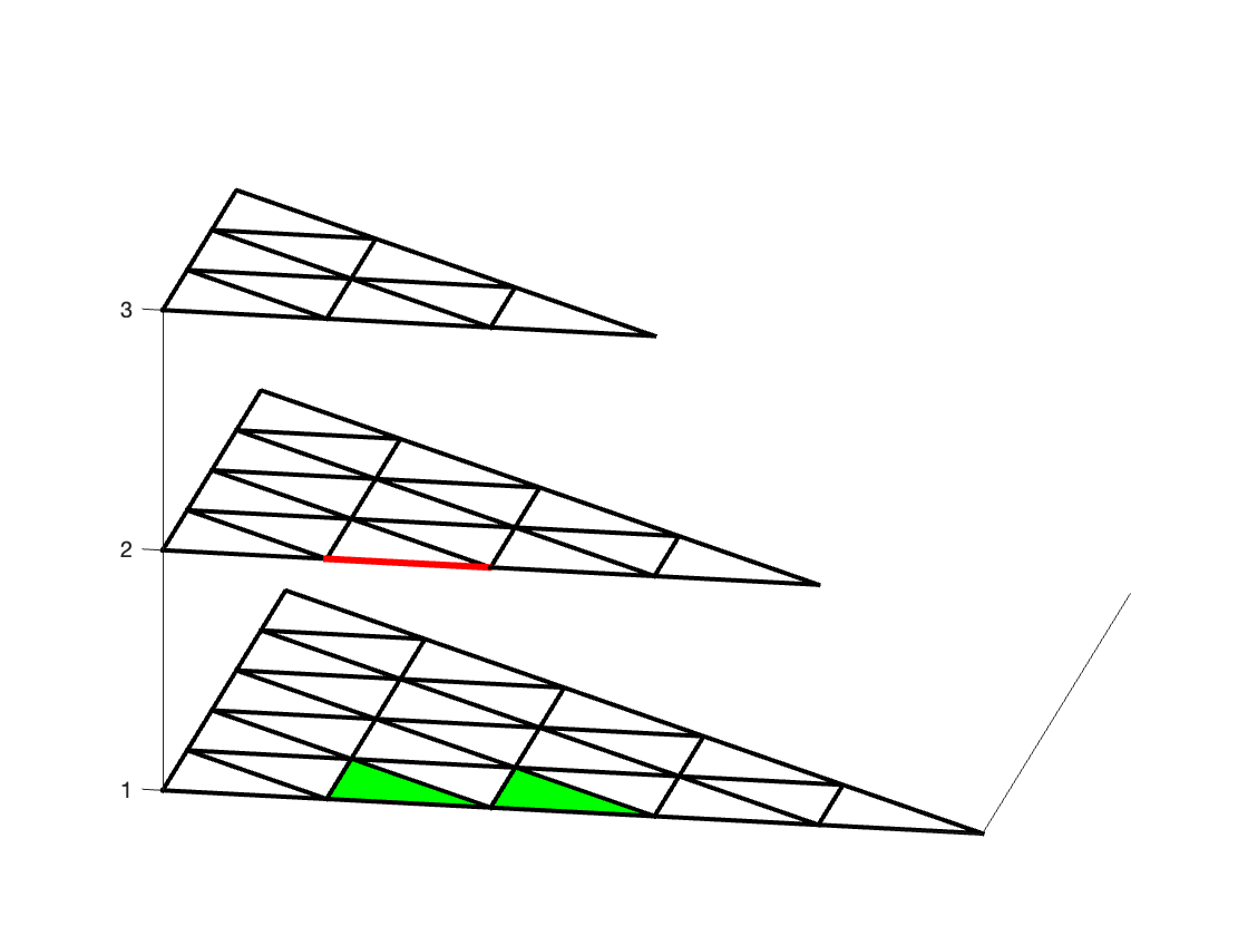
Figure 5. Geometric interpretation of the boundary function. Each layer corresponds to a single reduction of an $n$ grid. The red edge in layer 2 is determined by the edges of the green triangles in layer 1.

4.3. The Four $n$-grid functions with reduced arguments.

In this paper, we restrict ourselves solely to those triangles in the uniform center region. By Theorem 2.4 in the uniform center region, $T^{m}_{r,d,B}=T^{m}_{r,d,R}$ and $T^{m}_{r,d,e}=T^{m}_{r+1,d,e},e\in\{1,2,3\}$. Thus the boundary equation above is actually a function of only two edges, and the other three non-boundary equations are functions of only four edges. Moreover, it is no longer necessary to maintain both a right and a base equation (since those edge labels are always equal in the uniform center region) so we will retain only the function defining the right edge labels.

In summary, in this paper it suffices to use the following three functions when dealing with the uniform center region.

$$\text{BOUNDARY}(T^{m}_{r,1,L},T^{m}_{r,1,R})=T^{m+1}_{r,1,L},$$ (4.5)

$$\text{RIGHT}(T^{m}_{r,d,L},T^{m}_{r,d,R},T^{m}_{r,d+1,L},T^{m}_{r,d+1,R})=T^{m+1}_{r,d,R}$$ (4.6)

$$\text{LEFT}(T^{m}_{r,d-1,L},T^{m}_{r,d-1,R},T^{m}_{r,d,L},T^{m}_{r,d,R})=T^{m+1}_{r,d,L}$$ (4.7)

The arguments in (4.6)-(4.7) are formulated in terms of the resistances of edges in the triangular grid. For future reference we state a formulation in terms of $C^{X}.$ Such a formulation may be verified by inspecting Table 1.

$$\text{For odd $r,s\geq\frac{r+1}{2}$},C^{X}_{r+1,s}=\text{RIGHT}(C^{X}_{r,s-1},C^{X}_{r-1,s-1},C^{X}_{r-2,s-1},C^{X}_{r-3,s-1});$$ (4.8)

$$\text{for even $r,s\geq\frac{r}{2}+2$},C^{X}_{r,s}=\text{LEFT}(C^{X}_{r,s-1},C^{X}_{r-1,s-1},C^{X}_{r-2,s-1},C^{X}_{r-3,s-1}).$$ (4.9)

Comment 4.1.

For $s=\frac{r}{2}+1,$ the sequence $C_{r,s}=T^{s}_{r,1,L},\qquad r=0,1,2,\dotsc$ is the left-most diagonal of $C.$ The elements of this sequence are computed using the function BOUNDARY rather than the functions LEFT and RIGHT.

4.4. Boundary Conditions

To effectively use (4.8)-(4.9) we need the following fictitious boundary conditions.

$$\text{For $s\geq 1,$ and for $r\in\{-1,-2,-3\}$},C_{r,s}=1.$$ (4.10)

Example 4.2.

$C_{0,2}=LEFT(\frac{2}{3},1,1,1)=\frac{26}{27}$ and similarly $C_{1,2}=RIGHT(\frac{2}{3},1,1,1)=\frac{13}{12},$ $\frac{89}{100}=C_{2,3}=LEFT(\frac{1}{2},\frac{13}{13},\frac{26}{27},1),$ and $\frac{1157}{960}=C_{2,3}=LEFT(\frac{1}{2},\frac{13}{13},\frac{26}{27},1).$

Thus the boundary conditions allow application of (4.8)-(4.9) starting at row 0. These boundary conditions are fictitious in the precise sense that they don’t correspond to resistances of edges in a triangular grid.

4.5. Previous Results on Closed Forms

In [8] the following were proven.

$$\left\{C_{0,s}\right\}_{s\geq 1}=\left\{\frac{2}{3},\frac{26}{27},\frac{242}{243},\dotsc\right\}=\left\{1-\frac{3}{9^{s}}\right\}_{s\geq 1}=\left\{\frac{3\cdot 9^{s}-1}{3\cdot 9^{s}}\right\}_{s\geq 1},$$

and

$$\{C_{1,s}\}_{s\geq 2}=\left\{\frac{13}{12},\frac{121}{120},\frac{1093}{1092},\dotsc\right\}=\left\{\frac{3\cdot 9^{s}-1}{3\cdot 9^{s}-3}\right\}_{s\geq 2}.$$

5. An Illustrative Example

To assist the reader in familiarizing themselves with the computational methods presented in previous sections, including the definitions and theorems which can function as computational tools, we provide proof of the following illustrative claim, that uses all these methods.

claim:

$$C_{0,3}=\frac{242}{243},$$ (5.1)

that is the entry in row 0, column 3 of Table 2 is equal to $\frac{242}{243}$.

1. By comparing Table 2 and Table 1, $C_{0,3}$ corresponds to $T^{3}_{5,3,L}$, which implies, by our notational conventions, that $C_{0,3}$ is the left edge of

   $$\text{Row }r=5,\text{diagonal }d=3,\text{in the $s=3$rd reduction of the original all-one $n$-grid.}.$$ (5.2)

2. Therefore, computation of $C_{0,3}=T^{3}_{5,3,L},$ requires using (4.4), which requires consideration of the following 9 arguments,

   The resistance-edge labels in $$T^{2}_{5,2},T^{2}_{5,3}, T^{2}_{6,3}$$ and . (5.3)

3. To compute the resistance-edge labels of these three triangles, we use the Uniform Center Theorem (Theorem 2.4) which functions as a computational assistive tool. To use this theorem we first note that its inequalities have both lower and upper bounds. For purposes of computation, it suffices to assume $n$ sufficiently large such that all upper bounds are satisfied. The particular large value of $n$ chosen, does not affect the values in Table 2 since these values come from Table 1 and it is straightforward to verify that these values all lie in the uniform center (see Theorem 2.4).

4. Returning to the calculation of the 9 resistance labels of the three triangles in (5.3), by the Uniform Center Theorem, Part (i), we have $T^{2}_{5,3}=T^{2}_{6,3},$ and moreover, by Part (ii), the right and base sides of each of these triangles are equal. To see this, note that by Part (i) of the Uniform Center Theorem, the corresponding sides of two triangles are equal provided the underlying rows are at least as great as $s+d$ which by (5.2) equals 5. Similarly by Part (ii) the right and base edges of any triangle are equal provided the underlying row is at least as great as $2s-1$ which by (5.2) equals 5.

5. By (4.4) and (4.3), the computation of $T^{2}_{5,2}$ requires knowing resistance labels of $T^{1}_{5,1},T^{1}_{r,d},r\in\{5,6\},d\in\{2,3\}$.

We are now ready to obtain numbers.

• By (4.1)

  $$T^{1}_{5,1,L}=\Delta(1,1,1)+\Delta(1,1,1)=\frac{2}{3},$$ (5.4)

  where i) the fact that the arguments of the $\Delta$ equal one follow from the fact that $T^{0}$ is an all-one $n$ grid (Step A of Section 2.4) and the functional form of the $Delta$ function is given by (2.1).

• By Part (iii) of the Uniform Center Theorem (or by Comment 2.5), when $s=1$ the edge resistance labels of the interior edges of the triangle with top corner $T^{1}_{1,1}$ is 1 and hence

  $$T^{1}_{r,d},r\in\{5,6\},d\in\{2,3\}=1.$$ (5.5)

• Using the numerical values presented in (5.4)-(5.5), employing the computational definitions of $\Delta$ and $Y,$ (2.1), and by (4.4),

  $$T^{2}_{5,2,L}=Y\left(\Delta\left(1,1,\frac{2}{3}\right),\Delta(1,1,1),\Delta(1,1,1)\right)=\frac{26}{27},$$ (5.6)

• Finally, using the numerical values presented in (5.4)-(5.6), by (4.4),

  $$T^{3}_{5,3,L}=Y\left(\Delta\left(1,1,\frac{26}{27}\right),\Delta(1,1,1),\Delta(1,1,1)\right)=\frac{242}{243},$$ (5.7)

  confirming (5.1).

This establishes the claim and completes the illustrative example.

6. Annihilators

6.1. Overview

The main result of this paper identifies recursive patterns in the row sequences of $C^{X}$ and $C^{M}.$ Both the motivation and formulation of these results, as well as their proofs, require use of the method of annihilators [4, 5, 10].

As mentioned in Section 1.1, annihilator techniques were established by [4], are easy to use, and are a less messy approach to traditional inductive approaches in proofs connected with recursive sequences. Several authors [5, 10] have recently begun using them again when dealing with recursions. This section presents a complete, detailed, intuitive, but brief, description.

6.2. Review of Basic Terms

Consider a sequence, either over $\mathbb{Q}$ or $\mathbb{Q}[x].$ For example, Row 0, in Table 2, is $C_{0}=\{\frac{2}{3},\frac{26}{27},\frac{242}{243},\dotsc\}.$ A closed formula for this sequence is $1-\frac{3}{9^{i}}=\frac{N(i)}{D(i)}=\frac{9^{i}-3}{9^{i}},i=1,2,3,\dotsc.$ $N(i)$ and $D(i)$ satisfy recursions: $D(i)$ satisfies the (linear homogeneous) recursion with constant coefficients, $D_{i}=9D_{i-1},i\geq 2,$ and $N(i)=9^{i}-3$ satisfies both the non-homogeneous recursion, $N_{i}=9N_{i-1}+24,i\geq 2,$ and the homogeneous recursion $N_{i}=10N_{i-1}-9N_{i-2},i\geq 3.$ Every recursion has associated with it a characteristic polynomial. The characteristic polynomial for the underlying recursion of $D(i)$ is $X-9;$ the characteristic polynomial satisfied by the underlying (homogeneous) recursion of $N(i)$ is $X^{2}-10X+9=(X-9)(X-1).$

6.3. Annihilator Theory

Definition 6.1.

Given a sequence, $\mathbf{G}=\{G_{s}\}_{s\geq 0}$ (numerical or polynomial), the translation operator, $E,$ is defined for $s\geq 0,$ by $E(G_{s})=G_{s+1}.$

Defining addition and multiplication in the obvious manner, we have the following obvious result.

Lemma 6.2.

With $F$ any field (numerical or functional), $F[E]$ is an algebra over $F.$

Lemma 6.3.

The characteristic polynomial of a sequence, G, is also an annihilator of G,

Proof.

By interpreting the underlying variable of the characteristic polynomial as the translation operator, this result is straightforward to prove using the fact that the annihilators form an algebra over their underling field. ∎

Example 6.4.

Let $F=\{F_{s}\}_{s\geq 0},$ indicate the Fibonacci numbers, with characteristic polynomial $X^{2}-X-1.$ Then for $s\geq 0,$ $(E^{2}-E-1)[F_{s}]=E^{2}[F_{s}]-E[F_{s}]-F_{s}=F_{s+2}-F_{s+1}-F_{s}=0,$ the last equality following from the Fibonacci recursion.

To effectively use annihilators in proofs we will need two lemmas, one presenting trival facts and another dealing with sums and products. The proofs of these lemmas are also straightforward consequences of the fact that the annihilators form an algebra.

Lemma 6.5 (The Trivial Lemma).

i) $E-c$ annihilates the sequence $\{c^{s}\}_{s\geq 0},$ with $c$ an arbitrary constant.
ii) If $A$ annihilates the sequence $\textbf{G},$ then it also annihilates $aG+b$ for any constants $a,b.$

Lemma 6.6 (The Addition-Multiplication Lemma).

i) Suppose $A_{i},i\in I$ are annihilators of the sequences $\textbf{G}_{i},i\in I.$ Then $\sum_{i\in I}c_{i}G_{i}$ is annihilated by $\prod_{i\in I}A_{i},$ with the $c_{i}$ arbitrary constants.
ii)[12] Suppose $A_{i},i=1,2$ annihilate the sequences $\text{G}_{i}$ with characteristic polynomials, $p_{i}$ with roots $r_{i,j},1\leq j\leq k_{i},i=1,2.$ Then $A=\prod_{\text{all pairs $(i,j),(i^{\prime},j^{\prime})$}}(E-r_{i,j}r_{i^{\prime},j^{\prime}}),$ annihilates the (term by term) product $\textbf{G}_{1}\cdot\textbf{G}_{2}.$

Example 6.7.

Using the above machinery, we may calculate the annihilator of the function sequence G = $\{G_{s}=(3^{s}+2^{s})^{2}=9^{s}+4^{s}+2\cdot 6^{s}\}_{s\geq 0},$ as follows.

• $E-3$ and $E-2$ annihilate $\{3^{s}\}_{s\geq 0}$ and $\{2^{s}\}_{s\geq 0}$ respectively.

• Hence their product, $(E-3)(E-2)$ annihilates the sum $3^{s}+2^{s}.$

• Since $(E-3)(E-2)$ has roots $3,2$ we may obtain the annihilator of $(3^{s}+2^{s})^{2}$ by taking into consideration all products of pairs of roots: $(E-9)(E-6)(E-4).$

Remark 6.8.

In the sequel, when dealing with annihilators of powers, it is more readable to present the annihilator of the base of that power, it being understood that the annihilator of the power of the underlying base may be obtained by considering all pairs of products of roots.

7. The Main Theorem

This section motivates and states the main theorem of this paper for $C^{X}.$ Section 8 provides a corresponding motivation and statement for $C^{M}$. While, we do not provide complete proofs in this paper, we do i) motivate, state, and prove several initial cases, ii) showing a general proof technique capable of proving the theorem for any particular row in $C^{X},$ and iii) provide a conditional proof for $C^{X}_{i},i\text{ odd. }$ The complete proof requires development of more machinery than we originally anticipated. We hope to be able to present details in a follow-up paper.

An outline of this section is the following.

• Sections 7.1 - 7.2 present annihilators, closed forms, and underlying recursions for $C^{X}_{i},i=0,2$.

• Section 7.3 then notes that the annihilators have a clear pattern while the closed forms and underlying recursions do not. This immediately motivates statement of the main theorem of this paper for $C^{X}.$

• Known proof techniques for various cases are provided in sections 7.3 - 7.4.

7.1. The 0th and 1st rows, $C^{X}_{0},C^{X}_{1}$

By Table 3, $C^{X}_{0}=\frac{\frac{3}{9}X-1}{\frac{3}{9}X},\frac{3X-1}{3X},\frac{27X-1}{27X},\dotsc$. Table 5 provides 3 approaches to describing the underlying patterns associated with this sequence: annihilators, recursions, and closed forms. To illustrate use of the notation in this table, we first define

$$c_{0}(s,X)=\frac{c_{0,0}(s)X-c_{0,1}(s)}{c_{0,0}(s)X}=\frac{3\cdot 9^{s-2}X-1}{3\cdot 9^{s-2}X},$$ (7.1)

and then prove below that

$$c_{0}(s,X)=C_{0,s}^{X},\qquad s\geq 1.$$ (7.2)

To derive the entries in the table, note that given the closed formula for the coefficients, the annihilators follow immediately from Section 6.3. The recursions then follow from the annihilators using the well-known relationship between annihilators (characteristic polynomials) and recursions.

Therefore, to complete derivation of the table entries it suffices to prove (7.2). The inductive proof uses the method of computer verification [11]. For a base case we note that $c_{0}(1,X)=C^{X}_{0,1}.$ But then by the functions presented in Section 4, we verify

$$c_{0}(s+1,X)=LEFT(c_{0}(s,X),1,1,1),$$

completing the proof.

Since the functions in the sequence $C^{X}_{1}$ are a ratio of linear factors, the treatment of $C^{X}_{1}$ is similar to that of $C^{X}_{0}$ and hence omitted.

Table 5. Annihilators, recursions, and closed formula for coefficients of $X^{i},i=0,1$ of the sequence of numerators of $C^{X}_{0}.$

	Coef. of 1	Coef. of $X$
Annihilator	$(X-1)$	$(X-9)$
Recursion	$G_{n}=G_{n-1}$	$G_{n}=9G_{n-1}$
Closed form	$c_{0,0}(s)=1$	$c_{0,1}(s)=3\cdot 9^{s-2}$

For reference in Section 7.3 we note the closed form for $c_{1}(X,s).$

$$c_{1}(s,X)=\frac{3\cdot 9^{s-2}X-1}{3\cdot 9^{s-2}X-3}.$$ (7.3)

7.2. Row 2 of $C^{X},C^{X}_{2}$

The study of the sequence $C^{X}_{2}$ is similar to the treatment of $C^{X}_{0}$ just presented.

First, by Table 3

$$C_{2}^{X}=\left\{2\frac{2(1-\frac{4}{3}X+\frac{1}{3}X^{2})}{(X-1)^{2}},2\frac{13-36X+39X^{2}}{(9X-1)^{2}},2\frac{121-540X+3267X^{2}}{(81X-1)^{2}}\dotsc,\right\}.$$

Table 6 presents the annihilators (characteristic polynomials), recursions, and closed forms for the polynomial numerators of the members of $C^{X}_{2}.$ As noted in the discussion of Table 5, given the closed form, the annihilators follow from Section 6.3, and the recursions follow from the correspondence of characteristic polynomials and recursions. Therefore, to complete the proof, it suffices to verify

$$C_{2,s}^{X}=c_{2}(s,X),$$

with $c_{2}(s,X)$ defined by

$$c_{2}(s,X)=\frac{c_{2,0}(s)-c_{2,1}(s)X+c_{2,2}(s)X^{2}}{\left(9^{s-2}X-1\right)^{2}}.$$ (7.4)

The inductive proof uses verification: first we manually check that $c_{2}(X,3)=C^{X}_{2,3},$ thereby establishing a base case, and then verify, using the functions presented in Section 4, that

$$c_{2}(s+1,X)=LEFT(c_{2}(s,X),c_{1}(s,X),c_{0}(s,X),1)$$

with $c_{1}(s,X)$ defined by (7.3).

Table 6. Annihilators, recursions, and closed formula for coefficients of $X^{i},i=0,1,2$ in the numerators of $C_{2,i}^{X}$ and $C_{3,i}^{X}.$ Formulas are valid for $X\geq 3.$ Note that, annihilators and recursions are identical for $C^{X}_{2}$ and $C^{X}_{3}$

	Coef. of 1	Coef. of $X$	Coef. of $X^{2}$
Annihilator	$(X-1)(X-9)$	$(X-9)^{2}$	$(X-9)(X-81)$
Recursion	$G_{n}=10G_{n-1}+9G_{n-2}$	$G_{n}=18G_{n-1}+81G_{n-2}$	$G_{n}=90G_{n-1}-81G_{n-2}$
Closed form, $C^{X}_{2}$	$c_{2,0}(s)=27\cdot 9^{s-3}-1$	$c_{2,1}(s)=24\cdot(2s-3)\cdot 9^{s-3}$	$c_{2,2}(s)=81\cdot 81^{s-3}-3\cdot 9^{s-3}$

7.3. The Theorem

Tables 5 - 6 present 3 approaches to describing the sequences, $C^{X}_{0}i,i=0,1,2:$ annihilators, recursions, closed forms. By the same method used for these rows, similar tables can be produced for $C^{X}_{i},i=3,4,\dotsc.$ For a given $i,$ we explicitly list below the steps of the underlying algorithm:

• Generate the initial values of the sequence $C^{X}_{i},$ $C^{X}_{i,s},s=\lfloor\frac{i+1}{2}\rfloor+j,j=1,2,3,\dotsc,$ with $\lfloor x\rfloor$ denoting as usual the greatest integer function.

• Using these values conjecture the recursion, $c_{j,i}(s)$ satisfied by the coefficient sequences of $X^{j},j=0,1,\dotsc$

• After doing this for the numerator and denominator, form the conjectured function $c_{i}(s,X).$

• Perform verification: For $i$ even, verify

  $$c_{i}(s+1,X)=LEFT(c_{i}(s,X),c_{i-1}(s,X),c_{i-2}(s,X),c_{i-3}(s,X)),$$ (7.5)

  while for $i$ odd, verify

  $$c_{i}(s+1,X)=RIGHT(c_{i-1}(s,X),c_{i-2}(s,X),c_{i-3}(s,X),c_{i-4}(s,X)),$$ (7.6)

  thus completing the proof.

An examination of these tables shows no conspicuous pattern in the recursions or in the closed forms. Contrastively, the annihilators are a product of linear factors with roots $9^{\text{power}}.$ This motivates the main theorem of this paper.

Theorem 7.1 (Main Theorem).

For $i\geq 0,$ the roots of the annihilator of any of the coefficient sequences of the numerator and denominator of $C^{X}_{i}$ (or $C^{M}_{i})$ are all of the form $9^{\text{power}}.$

Example 7.2.

Table 6 presents the annihilators of the 3 coefficient sequences of the numerator of $C^{X}_{2}.$ As can be seen, the roots of these annihilators are $1,9,81,$ confirming the theorem.

7.4. Proofs

The previous section presented the inductive verification method for proving the Main Theorem for $C^{X}$ for $i=0,1,2,3,\dotsc.$ Using an induction approach, this verification approach would also prove (7.6). However, it would not work for (7.5) since the value of $c_{i}(X,s+1)$ depends on $c_{i}(X,s)$ which would lead to a circular induction assumption. It would appear that the verification methods using the functions presented in Section 4 are not sufficient to provide a proof. A possible alternate approach (which however also has not yielded results) is presented in Section 9

8. Multi-variate approach

In this section, we present results for $C^{M}$ analogous to the results presented in the previous section for $C^{X}.$ We have already indicated that the Main Theorem holds for $C^{M},$ that is, the roots of the annihilators of the coefficient sequences of its numerators or denominators (in any row) are powers of 9.

Following [7], $C^{M}$ and $C^{X}$ contrast with how they present closed formulas. The closed formulas for the circuit array $C^{X}$ while dependent on the values of $i$ and $s$ are functions of the single variable $X$. Contrastively, the closed formulas for the array $C^{M}$ are functions of multiple variables, $X_{1},X_{2},\dotsc,$ such that, as indicated in Section 3.7, upon substitution of $X_{i}$ with the numerical values of the leftside diagonal of $C$ we recover the corresponding numerical values in $C.$

More specifically, let $i$ be a given row and define $j=\lfloor i/2\rfloor+1$. Our intent is to write the values in row $i$ as functions of $X_{1},X_{2},\ldots,X_{j}$ with $X_{1}=C_{0,1},X_{2}=C_{2,2},\ldots,X_{j}=C_{2(j-1),j}.$ As just noted, these values in the numerical Circuit Array constitute the leftside and correspond to the left boundary edges on diagonal $d=1$ that appear in the reduction of the uniform center region of successive reductions of an all-one $n$-grid.

8.1. Row 0, $C^{M}_{0}$

Analogous to the development in Section 7.1, we i) define,

$$c^{M}_{0}(s,X_{1})=\frac{9^{s-1}-1+X_{1}}{9^{s-1}},\qquad s\geq 1,$$

and then, in Table 7, (ii) present the closed formulae, recursions, and annihilators of the coefficient sequences of the numerator and denominators of $C^{M}_{0}.$ As in the one-variable case, given the closed formula, a) the annihilators follow by the Trivial and Addition-Multiplication Lemmas of Section 6.3, b) the recursions follow from the annihilators, and c) proof of the closed form follows from a straightforward inductive proof verifying $c^{M}_{0}(s+1,X_{1})-LEFT(c^{M}_{0}(s,X_{1}),1,1,1)=0.$

The Main Theorem as applied to $C^{M}$ is confirmed for row 0: the annihilators of the coefficient sequences of the numerator (or denominator) only have roots which are powers of 9.

Moreover, by an adaptation of the bulleted technique presented in Section 7.3, it can be shown that the closed form for $c^{M}_{1}(s,X_{1})$ is

$$c^{M}_{1}(s,X_{1})=\frac{(9^{s-1}-1)+X_{1}}{3(X_{1}+3\cdot 9^{s-2}-1)},\qquad s\geq 2.$$ (8.1)

The annihilators of the coefficient sequences of $1$ and $X_{1}$ are similar to those for the case $C^{M}_{0}$ and conform to the expected belavior indicated by the Main Theorem.

Table 7. Annihilators, recursions, and closed formula for coefficients of $X_{1}^{s},s=0,1$ of the numerators of $C^{M}_{0}.$

	Coef. of 1	Coef. of $X_{1}$
Annihilator	$(X-1)$	$(X-1)(X-9)$
Recursion	$G_{n}=G_{n-1}$	$G_{n}=10G_{n-1}-9G_{n-2}$
Closed form	$c_{0,0}=1$	$c_{0,1}(s)=9^{s-1}-1$

8.2. Row 2 of $C^{M},C^{M}_{2}$

Row $C^{M}_{2}$ is significantly more complex. We define coefficient functions,

$$c_{2,1}(s)=9^{s-2}$$

$$c_{2,0}(s)=9^{s-2}-1$$

$$c_{1,1}(s)=4\cdot 9^{s-2}$$

$$c_{1,0}(s)=2+(16(s-2)-2)9^{s-2}$$

$$c_{0,1}(s)=4\cdot 9^{s-2}$$

$$c_{0,0}(s)=-1+9\cdot 81^{s-2}-(8+16(s-2))9^{s-2}$$

$$c_{i,j}(s)=0,\text{otherwise}.$$

By the Trivial and Addition-Multiplication Lemma of Section 6.3 these coefficient functions satisfy the recursions presented in Table 8.

Using these functions define

$$c^{M}_{2}(s,X_{1},X_{2})=\frac{\displaystyle\sum_{0\leq i,j\leq 2}c_{i,j}(s)X_{1}^{i}X_{2}^{j}}{(3\cdot 9^{s-2}-1+X_{1})^{2}}.$$

To prove

$$C_{s,2}^{M}=c_{2}^{M}(s,X_{1},X_{2}),$$

we follow the bulleted procedure presented in Section 7.3. The inductive proof observes that this equality is satisfied if $s=3,$ and then using an induction assumption we verify that

$$c_{2}^{M}(s+1,X_{1},X_{2})-LEFT(c_{2}^{M}(s,X_{1},X_{2}),c^{M}_{1}(X_{1},s),c_{0}^{M}(s,X_{1}),1)=0.$$

Coefficient	Recursion	Characteristic Polynomial
$X_{1}^{0}X_{2}^{0}$	$G_{s}=100G_{s-1}-1638G_{s-2}+8100G_{s-3}-6561G_{s-4}$	$(X-81)(X-9)^{2}(X-1)$
$X_{1}^{0}X_{2}^{1}$	$G_{n}=10G_{s-1}-G_{s-2}$	$(X-1)(X-9)$
$X_{1}^{1}X_{2}^{0}$	$G_{s}=19G_{s-1}-99G_{s-2}+81G_{s-3}$	$(X-9)^{2}(X-1)$
$X_{1}^{1}X_{2}^{1}$	$G_{n}=9G_{s-1}$	$(X-9)$
$X_{1}^{2}X_{2}^{0}$	$G_{n}=10G_{s-1}-9G_{s-2}$	$(X-1)(X-9)$
$X_{1}^{2}X_{2}^{1}$	$G_{s}=9G_{s-1}$	$(X-9)$

Table 8. The recursions satisfied by the coefficients of the numerator of $C^{M}_{2,s}$.

Comment 8.1.

$C^{M}$ has similar issues to $C^{X}:$ i) we can prove the Main Theorem for any row where we first calculate the closed form, ii) we can prove the Main Theorem for odd rows provided the Main Theorem is known to hold for the previous rows, iii) attempts to prove the Main Theorem for even rows have not produced any results.

We also note that earlier versions of this paper concentrated on recursions (either non-homogeneous or homogeneous) for the numerators and denominators proper (vs. their coefficient sequences). Howeveer we abandoned this approach upon realizing that the characteristic polymomial satisfied by a polynomial sequence is the least common multiple of the characteristic polynomials of its coefficient sequences (This follows from the methods in Section 6.3).

For example, let $N(s,X_{1},X_{2})=\sum_{0\leq i,j\leq 2}c_{i,j}(s)X_{1}^{i}X_{2}^{j},$ the numerator of $C^{M}_{s}.$ Then $N$ satisfies the following non-homogeneous recursion:

$$N(s+1,X_{1},X_{2})=8(9^{s}-1+X_{1})^{2}+9N(s,X_{1},X_{2}).$$

This can be proven by checking some initial case and then verifying that the difference of sides equals 0.

9. The Hiccup Conjectures

Several attempts were made to prove the Main Theorem for even rows. One very simple pattern emerged, which deserves attention in its own right. We first present some motivation.

9.1. Motivation Examples

Consider

$$C^{X}_{3,4} = \frac{(-1+27X)(121-540X+3267X^{2})}{24(-1+81X)(5-18X+45X^{2})}$$

$$C^{X}_{4,4} = \frac{(-1+27X)(-89+333X-447X^{2}+267X^{3})}{(5-18X+45X^{2})^{2}}$$

$$C^{X}_{5,4} = \frac{(13-36X+39X^{2})(-89+333X-447X^{2}+267X^{3})}{192(-1+X)^{3}(5-18X+45X^{2})}$$

Several patterns emerge.

• Each Circuit Array element is a ratio of products of two polynomials (with an extra constant term)

• The same linear factor occurs in $C^{X}_{3,4},C^{X}_{4,4}$

• The same cubic factor occurs in $C^{X}_{4,4},C^{X}_{5,4}$

• The same quadratic factor appears in the denominator of all three elements, however it is squared in $C^{X}_{4,4}$.

These patterns constitute the content of the hiccup conjecture and its collorary. The importance of these observations is that the Main Theorem which was formulated in terms of the coefficient sequences of the numerators and denominators of elements of the Circuit Array, also applies to the multiplicand families making up the numerators and denominators. This eases proofs since we are showing a recursive realtionship on two multiplicands each of a much lower degree than their product.

9.2. The Formulation

We use the notation $P_{r,d}$ ($Q_{r,d}$) to refer to some polynomial of degree $d$ in the numerator (resp. denominator) of elements in row $C^{X}_{r}.$ (The notation is deliberately ambiguous since $P_{r,d}$ or $Q_{r,d}$ could refer to two different polynomials in two different rows. Issues of distinctness will be addressed after statement of the conjectures.)

Conjecture 9.1 (Hiccup).

i) For $2n-1\geq 3,$ for each $\ell$ where $C^{X}_{2n-1,\ell}$ is defined, there is a polynomial, $Q_{2n+i,n},i\in\{-1,0,1\},$ of degree $n$, such that, $(Q_{2n+i,n})^{k_{i}},\;k_{0}=2,k_{\pm 1}=1,$ divides the denominator of $C^{X}_{2n+i,\ell}.$
ii) For $2n-1\geq 3,$ for each $j$ where $C^{X}_{2n+i,j}$ is defined, there exists a polynomial,$P_{2n+i,n-1},i\in\{-1,0\}$ of degree $n-1,$ such that $P_{2n+i,n-1},$ divides the numerator of $C^{X}_{2n+i,j}$ and
iii) For $2n\geq 4,$ for each $j$ where $C^{X}_{2n+i,j},i\in\{0,1\}$ is defined, $P_{2n+i,n+1},$ divides the numerator of $C^{X}_{2n+i,j}.$
iv) Except for constant factors, there are no other factors for the numerators and denominators mentioned in previous parts of the conjecture.

Corollary 9.2.

For $n\geq 3$, up to a constant factor, $C^{X}_{n,j}$ (where defined), is a ratio of products of two polynomial factors.

Proof.

Clear. ∎

Since the conjecture did not lead to a proof of the main theorem,we only briefly illustrate further aspects of the conjecture without developing a formalism. Notice that the three quadratic polynomials in the denominators of the motivating examples corresponding to Part i) of the conjecture, which all lie in column 4 of $C^{X},$ are identical. Also notice that the two linear or two cubic factors in the numerators of the motivating examples corresponding to Parts ii) and iii) of the conjecture, which all lie in Column 4 of $C^{X},$ are identical.

To further develop our point we consider $C_{i,6},i\in\{4,5,7,8\}.$ According to the conjecture, cubic polynomials are factors of $C_{i,6},i=4,5$; these two cubic polymomials are identical. Cubic polynomials are also factors of $C_{i,6},i=7,8$; these two cubic polymomials are identical. However the cubic polynomials that is a factor for $C_{i,6},i=7,8$ is different than the cubic factor that is a factor of the numerators of $C_{i,6},i=4,5.$

Although these two cubic polynomials are different, i) they are consecutive members of the cubic factors dividing the sequence $C_{4,j},j=3,4,5,\dotsc.$ ii) Moreover, consistent with the main theorem (which technically only applies to entire numerators and denominators) this sequence of cubic factors are a recursive sequence whose annihilator has roots that are exclusively powers of 9.

Because of these considerations, to prove the Main Theorem (which technically applies to entire numerators and denominators) it suffices to prove the main theorem for the factors of the numerators and denominators. While this observation led to some hope we are still unable to completely prove either the hiccup conjectures or the Main Theorem.

Finally we explain the name, hiccup, which of course is mnemonical. As just mentioned rows 4,5,7,8 but not 6 have cubic factors; these cubic factors, which divide the numerators of the polynomial sequence in the numerators of $C^{X}_{4},$ satisfy a recursive relationship whose underlying characteristic polynomial has roots exclusively powers of 9. If one says 4,5,7,8 and skips 6 it sounds like a hiccup: One says, 4,5, hiccups, and continues with 7,8. Similarly if one says 3,4,5 which have the quadratic factor in the denominators of $C^{X}_{i,4},i\in\{3,4,5\}$ and hiccups when saying the 4, the 4 will be emphasized corresponding to the square of the quadratic factor.

10. Conclusion

This paper has explored the polynomial sequences of the Circuit Array which are polynomial generalizations of the numerical values of edge-resistances occurring in the center of the collection of $n$-grids and its reductions. Interesting simply stated patterns exhibit themselves some of which we have proved. We believe this to be a fertile ground for future research.

References

- [1] R. B. Bapat and Somit Gupta. Resistance distance in wheels and fans. Indian. J. Pure App. Math., 41(1):1–13, Feb 2010.
- [2] Wayne Barrett, Emily. J. Evans, and Amanda E. Francis. Resistance distance in straight linear 2-trees. Discrete Appl. Math., 258:13–34, 2019.
- [3] Wayne Barrett, Emily J. Evans, and Amanda E. Francis. Resistance distance and spanning 2-forest matrices of linear 2-trees. Linear Algebra Appl., 606:41–67, 2020.
- [4] George Boole. A Treatise on the Calculus of Finite Differences. Cosimo, New York, 2007.
- [5] Duane DeTemple and William Webb. Combinatorial Reasoning: An Introduction to the Art of Counting. Wiley,Hoboken:NJ, 2014.
- [6] Peter G. Doyle and J. Laurie Snell. Random Walks and Electric Networks, The Carus Mathematical Monographs, Volume 22, Washington, DC: MAA, 1988
- [7] E. J. Evans and R. J. Hendel. An infinite 2-dimensional array associated with electric circuits. The Fibonacci Quarterly, 60(5):151–171, Dec 2022.
- [8] E. J. Evans and R. J. Hendel, Resistance values under transformations in regular triangular grids, http://arxiv.org/abs/2207.11207, 2022.
- [9] E.J. Evans and A.E. Francis. Algorithmic techniques for finding resistance distances on structured graphs. Discrete Applied Mathematics, 320:387–407, 2022.
- [10] Russell Jay Hendel. Continued fractions consisting of alternating string functions. Proceedings of the 14th Fibonacci Conference, pages 123–139, 2011.
- [11] Russell Jay Hendel. Limiting behavior of resistances in triangular graphs. https://arxiv.org/abs/2109.01959, 2021.
- [12] Dov Jarden. Recurring sequences; A collection of Papers (3rd Edition). Riveon LeMathematica, Jerusalem:Israel, 1973.
- [13] J. H. Loxton and A. J. Van der Poorten. Transcendence and algebraic independence by a method of mahler. transcendence theory: advances and applications. Proc. Conf., Univ. Cambridge, pages 211–226, 1976.
- [14] Peter Roquette. The Riemann hypothesis in characteristic in historical perspective, volume 2222 of Lecture Notes in Mathematics. Springer, Cham, 2018. History of Mathematics Subseries.