Inverse Kinematics and Path Planning of Manipulator Using Real Quantifier Elimination Based on Comprehensive Gröbner Systems

Abstract

Methods for inverse kinematics computation and path planning of a three degree-of-freedom (DOF) manipulator using the algorithm for quantifier elimination based on Comprehensive Gröbner Systems (CGS), called CGS-QE method, are proposed. The first method for solving the inverse kinematics problem employs counting the real roots of a system of polynomial equations to verify the solution’s existence. In the second method for trajectory planning of the manipulator, the use of CGS guarantees the existence of an inverse kinematics solution. Moreover, it makes the algorithm more efficient by preventing repeated computation of Gröbner basis. In the third method for path planning of the manipulator, for a path of the motion given as a function of a parameter, the CGS-QE method verifies the whole path’s feasibility. Computational examples and an experiment are provided to illustrate the effectiveness of the proposed methods.

1 Introduction

We discuss inverse kinematics computation of a 3-degree-of-freedom (DOF) manipulator using computer algebra. Manipulator is a robot with links and joints that are connected alternatively. The end part is called the end-effector. The inverse kinematics problem is fundamental in motion planning. In the motion planning of manipulators, a mapping from a joint space and the operational space of the end-effector is considered for solving the forward and inverse kinematics problems. The forward kinematics problem is solved to find the end-effector’s position from the given configuration of the joints. On the other hand, the inverse kinematic problem is solved to find the configuration of the joints if the solution exists.

For solving inverse kinematics problems, computer algebra methods have been proposed [5, 8, 17, 20, 21]. Some of these methods are especially for modern manipulators with large degrees of freedom [17], which indicates an interest in applying global methods to a real-world problem. The inverse kinematics problem is expressed as a system of polynomial equations in which trigonometric functions are replaced with variables, and constraints on the trigonometric functions are added as new equations. Then, the system of equations gets “triangularized” by computing a Gröbner basis and approximate solutions are calculated using appropriate solvers. We have proposed an implementation for inverse kinematics computation of a 3-DOF manipulator [7]. The implementation uses SymPy, a library of computer algebra, on top of Python, and also uses a computer algebra system Risa/Asir [13] for Gröbner basis computation, connected with OpenXM infrastructure [11].

An advantage of using Gröbner basis computation for solving inverse kinematics problems is that the global solution can be obtained. The global solution helps to characterize the robot’s motion, such as kinematic singularities. On the other hand, Gröbner basis computation is relatively costly. Thus, repeating Gröbner basis computation every time the position of the end-effector changes leads to an increase in computational cost. Furthermore, in inverse kinematics computation with a global method, it is necessary to determine if moving the end-effector to a given destination is feasible. Usually, numerical methods are used to compute an approximate solution of the system of polynomial equations, but this is only an approximation and another computation is required to verify the existence of the solution to the inverse kinematics problem. In fact, our previous implementation above has the problem of calculating approximate solutions without verifying the existence of the real solution to the inverse kinematics problem.

We have focused on Comprehensive Gröbner Systems (CGS). CGS is a theory and method for computing Gröbner bases for ideals of the polynomial ring, where generators of the ideal have parameters in their coefficients. Gröbner basis is computed in different forms depending on constraints of parameters. In the system of polynomial equations given as an inverse kinematics problem, by expressing the coordinates of the end-effector as parameters, then, by computing CGS from the polynomial system, we obtain the Gröbner basis where the coordinates of the end-effector are expressed in terms of parameters. When moving the robot, the coordinates of the end-effector are substituted into the Gröbner basis corresponding to the segment in which the coordinates satisfy constraints on the parameters, then solved the configuration of the joints. This allows us to solve the system of polynomial equations immediately without computing Gröbner basis when the robot is actually in motion.

Furthermore, we have focused on quantifier elimination with CGS (CGS-QE) [6]. CGS-QE is a QE method based on CGS, and it is said to be effective when the constraints have mainly equality constraints. When we use CGS to solve inverse kinematics problems for the above purposes, the CGS-QE method also allows us to verify the existence of a solution to the inverse kinematics problem. Then, if the given inverse kinematic problem is determined to be feasible, it is possible to immediately obtain a solution to the inverse kinematic problem without Gröbner basis computation.

With these motivations, we have proposed an inverse kinematics solver that verifies the existence of a solution to the inverse kinematics problem by the CGS-QE method, and efficiently finds a feasible solution using CGS [14]. Our solver uses “preprocessing steps [14, Algorithm 1]” to configure the solver before the startup of the manipulator, that is, we eliminate segments without real points and, if the input system is a non-zero dimensional ideal, we find a trivial root that makes the input system zero-dimensional. Then, when the manipulator is running, the solver uses “main steps [14, Algorithm 2]” to determine the existence of feasible solutions and compute them. However, in the proposed algorithm, the preprocessing steps were performed manually.

The main contribution of this paper is the extension of our previous solver [14] in two ways. The first is that the computation of the preprocessing steps is completely automated. The procedures in the previous work were refined into an algorithm that can be executed automatically. The second is the extension of the solver to path planning (trajectory planning) in two ways.

Trajectory planning is a computation in which the path along which the manipulator (the end-effector) is to be moved is given in advance, and the configuration of the joints is determined at each time so that the position of the end-effector changes as a function of time along that path. Trajectory planning also considers the manipulator’s kinematic constraints to determine the configuration of the joints at each time.

Our extension of the solver to trajectory planning is as follows. The first method iteratively solves the inverse kinematics problem along a path using the proposed method described above. In the second method, the path is represented by a function of a parameter. Feasibility of the inverse kinematics problem is determined using the CGS-QE method within a given time range. It determines whether the entire trajectory falls within the manipulator’s feasible region before the manipulator moves. If the trajectory planning is feasible, we solve the inverse kinematics problem sequentially along the path.

This paper is organized as follows. In Sect. 2, the inverse kinematics problem for the 3-DOF manipulator is formulated for the use of Gröbner basis computation. In Sect. 3, CGS, CGS-QE method, and a method of real root counting are reviewed. In Sect. 4, an extension of a solver for inverse kinematics problem based on the CGS-QE method is proposed. In Sect. 5, trajectory planning methods based on the CGS-QE method are presented. In Sect. 6, conclusions and future research topics are discussed.

2 Inverse Kinematics of a 3-DOF Robot Manipulator

In this paper, as an example of a 3-DOF manipulator, one built with LEGO^® MINDSTORMS^® EV3 Education (henceforth abbreviated to EV3) is used (Fig. 1).

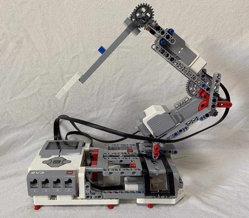
Figure 1: A 3-DOF manipulator built with EV3.

The EV3 kit is equipped with large and small motors, optical, touch, gyro sensors, and a computer called “EV3 Intelligent Brick.” A GUI-based development environment is provided, and development environment with Python, Ruby, C, and Java are also available.

The components of the manipulator is shown in Fig. 2.

Figure 2: Components and the coordinate systems of the manipulator.

The manipulator has eight links (segments) and eight joints connected alternatively. A link fixed to the bottom is called Link $0$, and the other links are numbered as Link $1,\dots,7$ towards the end-effector. For $j=1,\dots,7$, the joint connecting Links $j-1$ and $j$ is called Joint $j$. The foot of Link $0$ on the ground is called Joint $0$, and the end-effector is called Joint $8$. Due to the circumstances of the appropriate coordinate transformation described below, Joints $1$ and $2$ overlap, and Link $1$ does not exist either. (Note that by setting joint parameters appropriately, the consistency of coordinate transformation is maintained even for such a combination of links and segments.) Joints $1(=2),4,7$ are revolute joints, while the other joints are fixed.

At Joint $i$, according to a modified Denavit-Hartenberg convention [16], the coordinate system $\mathrm{\Sigma}_{i}$ is defined as follows (Fig. 2). The origin is located at Joint $i$, and the $x_{i}$, $y_{i}$ and $z_{i}$ axes are defined as follows (in Fig. 2, the positive axis pointing upwards and downwards is denoted by “$\odot$” and “$\otimes$”, respectively):

• The $z_{j}$ axis is chosen along with the axis of rotation of Joint $j$.

• The $x_{j-1}$ axis is selected along with the common normal to axes $z_{j-1}$ to $z_{j}$.

• The $y_{j}$ axis is chosen so that the present coordinate system is right-handed.

Note that the above definition of axes may have ambiguity. For the current manipulator, if the axes $z_{i}$ and $z_{i-1}$ are parallel, there are infinite ways to take the $x_{i}$ axis. Thus, in this case, the $x_{i}$ axis is defined as follows.

• In the coordinate system $\mathrm{\Sigma}_{0}$, define the axes $x_{0},y_{0},z_{0}$ like those in $\mathrm{\Sigma}_{1}$ as depicted in Fig. 2. Also, in the coordinate system $\mathrm{\Sigma}_{8}$, define the axes $x_{8},y_{8},z_{8}$ like those in $\mathrm{\Sigma}_{7}$, respectively.

• In the coordinate system $\mathrm{\Sigma}_{i}$ ($i=2,\dots,7$), since the origin is located on Joint $i$, define the $x_{i}$ axis to overlap Link $i$.

For analyzing the motion of the manipulator, we define a map between the joint space and the configuration space or operational space. For a joint space, since we have revolute joints $1,4,7$, their angles $\theta_{1},\theta_{4},\theta_{7}$, respectively, are located in a circle $S^{1}$, we define the joint space as $\mathcal{J}=S^{1}\times S^{1}\times S^{1}$. For a configuration space, let $(x,y,z)$ be the end-effector position located in $\mathbb{R}^{3}$ and then define the configuration space as $\mathcal{C}=\mathbb{R}^{3}$. Thus, we consider a map $f:\mathcal{J}\longrightarrow\mathcal{C}$. The forward kinematic problem is to find the position of the end-effector in $\mathcal{C}$ for the given configuration of the joints in $\mathcal{J}$, while the inverse kinematic problem is to find the configuration of the joints in $\mathcal{J}$ which enables the given position of the end-effector in $\mathcal{C}$. We first solve the forward kinematic problem for formulating the inverse kinematic problem.

Let $a_{i}$ be the distance between axes $z_{i-1}$ and $z_{i}$, $\alpha_{i}$ the angle between axes $z_{i-1}$ and $z_{i}$ with respect to the $x_{i}$ axis, $d_{i}$ the distance between the axes $x_{i-1}$ and $x_{i}$, and $\theta_{i}$ be the angle between the axes $x_{i-1}$ and $x_{i}$ with respect to the $z_{i}$ axis. Then, the coordinate transformation matrix ${}^{i-1}T_{i}$ from the coordinate system $\mathrm{\Sigma}_{i}$ to $\mathrm{\Sigma}_{i-1}$ is expressed as in Fig. 3.

$${}^{i-1}T_{i} =\begin{pmatrix}1&0&0&a_{i}\\ 0&1&0&0\\ 0&0&1&0\\ 0&0&0&1\end{pmatrix}\begin{pmatrix}1&0&0&0\\ 0&\cos\alpha_{i}&-\sin\alpha_{i}&0\\ 0&\sin\alpha_{i}&\cos\alpha_{i}&0\\ 0&0&0&1\end{pmatrix}\begin{pmatrix}1&0&0&0\\ 0&1&0&0\\ 0&0&1&d_{i}\\ 0&0&0&1\end{pmatrix}\begin{pmatrix}\cos\theta_{i}&-\sin\theta_{i}&0&0\\ \sin\theta_{i}&\cos\theta_{i}&0&0\\ 0&0&1&0\\ 0&0&0&1\end{pmatrix}$$

$$=\begin{pmatrix}\cos\theta_{i}&-\sin\theta_{i}&0&a_{i}\\ \cos\alpha_{i}\sin\theta_{i}&\cos\alpha_{i}\cos\theta_{i}&-\sin\alpha_{i}&-d_{i}\sin\alpha_{i}\\ \sin\alpha_{i}\sin\theta_{i}&\sin\alpha_{i}\cos\theta_{i}&\cos\alpha_{i}&d_{i}\cos\alpha_{i}\\ 0&0&0&1\end{pmatrix},$$

Figure 3: The transformation matrix ${}^{i-1}T_{i}$.

where the joint parameters $a_{i}$, $\alpha_{i}$, $d_{i}$ and $\theta_{i}$ are shown in Table 1 (note that the unit of $a_{i}$ and $d_{i}$ is [mm]).

Table 1: Joint parameters for EV3.

$i$	$a_{i}$ (mm)	$\alpha_{i}$	$d_{i}$ (mm)	$\theta_{i}$
1	0	0	80	$\theta_{1}$
2	0	$\pi/2$	0	$\pi/4$
3	${88}$	0	0	$\pi/4$
4	${24}$	0	0	$\theta_{4}$
5	${96}$	0	0	$-\pi/2$
6	${16}$	0	0	$\pi/2$
7	${40}$	0	0	$\theta_{7}$
8	${120}$	0	0	0

The transformation matrix $T$ from the coordinate system $\mathrm{\Sigma}_{8}$ to $\mathrm{\Sigma}_{0}$ is calculated as $T={}^{0}T_{1}{}^{1}T_{2}{}^{2}T_{3}{}^{3}T_{4}{}^{4}T_{5}{}^{5}T_{6}{}^{6}T_{7}{}^{7}T_{8}$, where ${}^{i-1}T_{i}$ is expressed as in Fig. 4.

$${}^{0}T_{1} =\left(\begin{array}[]{cccc}\cos\theta_{1}&-\sin\theta_{1}&0&0\\ \sin\theta_{1}&\cos\theta_{1}&0&0\\ 0&0&1&80\\ 0&0&0&1\end{array}\right), {}^{1}T_{2} =\left(\begin{array}[]{cccc}\frac{\sqrt{2}}{2}&-\frac{\sqrt{2}}{2}&0&0\\ 0&0&-1&0\\ \frac{\sqrt{2}}{2}&\frac{\sqrt{2}}{2}&0&0\\ 0&0&0&1\end{array}\right), {}^{2}T_{3} =\left(\begin{array}[]{cccc}\frac{\sqrt{2}}{2}&-\frac{\sqrt{2}}{2}&0&{88}\\ \frac{\sqrt{2}}{2}&\frac{\sqrt{2}}{2}&0&0\\ 0&0&1&0\\ 0&0&0&1\end{array}\right),$$

$${}^{3}T_{4} =\left(\begin{array}[]{cccc}\cos\theta_{4}&-\sin\theta_{4}&0&{24}\\ \sin\theta_{4}&\cos\theta_{4}&0&0\\ 0&0&1&0\\ 0&0&0&1\end{array}\right), {}^{4}T_{5} =\left(\begin{array}[]{cccc}0&1&0&{96}\\ -1&0&0&0\\ 0&0&1&0\\ 0&0&0&1\end{array}\right), {}^{5}T_{6} =\left(\begin{array}[]{cccc}0&-1&0&{16}\\ 1&0&0&0\\ 0&0&1&0\\ 0&0&0&1\end{array}\right),$$

$${}^{6}T_{7} =\left(\begin{array}[]{cccc}\cos\theta_{7}&-\sin\theta_{7}&0&{40}\\ \sin\theta_{7}&\cos\theta_{7}&0&0\\ 0&0&1&0\\ 0&0&0&1\end{array}\right), {}^{7}T_{8} =\left(\begin{array}[]{cccc}1&0&0&{120}\\ 0&1&0&0\\ 0&0&1&0\\ 0&0&0&1\end{array}\right).$$

Figure 4: The transformation matrix ${}^{i-1}T_{i}$ ($i=1,\dots,8$).

Then, the position $(x,y,z)$ of the end-effector with respect to the coordinate system $\mathrm{\Sigma}_{0}$ is expressed as

$$\begin{split}x&=-120\cos{\theta_{1}}\cos{\theta_{4}}\sin{\theta_{7}}+16\cos{\theta_{1}}\cos{\theta_{4}}-120\cos{\theta_{1}}\sin{\theta_{4}}\cos{\theta_{7}}\\ &\qquad-136{\cos}\theta_{1}{\sin}\theta_{4}+44{\sqrt{2}}\cos{\theta_{1}},\\ y&=-120\sin{\theta_{1}}\cos{\theta_{4}}\sin{\theta_{7}}+16\sin{\theta_{1}}\cos{\theta_{4}}-120\sin{\theta_{1}}\sin{\theta_{4}}\cos{\theta_{7}}\\ &\qquad-136\sin{\theta_{1}}\sin{\theta_{4}}+44{\sqrt{2}}\sin{\theta_{1}},\\ z&=120\cos{\theta_{4}}\cos{\theta_{7}}+136{\cos}{\theta_{4}}-120\sin{\theta_{4}}\sin{\theta_{7}}+16{\sin}{\theta_{4}}+104+44{\sqrt{2}}.\end{split}$$ (1)

The inverse kinematics problem comes down to solving 1 for $\theta_{1}$, $\theta_{4}$, $\theta_{7}$. By substituting trigonometric functions $\cos\theta_{i}$ and $\sin\theta_{i}$ with variables as $c_{i}=\cos\theta_{i},s_{i}=\sin\theta_{i},$ subject to $c_{i}^{2}+s_{i}^{2}=1$, 1 is transferred to a system of polynomial equations:

$$\begin{split}f_{1}&=120c_{1}c_{4}s_{7}-16c_{1}c_{4}+120c_{1}s_{4}c_{7}+136c_{1}s_{4}-44{\sqrt{2}}c_{1}+x=0,\\ f_{2}&=120s_{1}c_{4}s_{7}-16s_{1}c_{4}+120s_{1}s_{4}c_{7}+136s_{1}s_{4}-44{\sqrt{2}}s_{1}+y=0,\\ f_{3}&=-120c_{4}c_{7}-136c_{4}+120s_{4}s_{7}-16s_{4}-104-44{\sqrt{2}}+z=0,\\ f_{4}&=s_{1}^{2}+c_{1}^{2}-1=0,\quad f_{5}=s_{4}^{2}+c_{4}^{2}-1=0,\quad f_{6}=s_{7}^{2}+c_{7}^{2}-1=0.\end{split}$$ (2)

3 Real Quantifier Elimination Based on CGS

Equations (1) and (2) show that solving the inverse kinematic problem for the given system can be regarded as a real quantifier elimination of a quantified formula

$$\exists{c_{1}}\exists{s_{1}}\exists{c_{4}}\exists{s_{4}}\exists{c_{7}}\exists{s_{7}}\\ (f_{1}=0\land f_{2}=0\land f_{3}=0\land f_{4}=0\land f_{5}=0\land f_{6}=0),$$ (3)

with $x,y,z$ as parameters.

In this section, we briefly review an algorithm of real quantifier elimination based on CGS, the CGS-QE algorithm, by Fukasaku et al. [6]. Two main tools play a crucial role in the algorithm: one is CGS, and another is real root counting, or counting the number of real roots of a system of polynomial equations. Note that, in this paper, we only consider equations in the quantified formula.

Hereafter, let $R$ be a real closed field, $C$ be the algebraic closure of $R$, and $K$ be a computable subfield of $R$. This paper considers $R$ as the field of real numbers $\mathbb{R}$, $C$ as the field of complex numbers $\mathbb{C}$, and $K$ as the field of rational numbers $\mathbb{Q}$. Let $\bar{X}$ and $\bar{A}$ denote variables $X_{1},\dots,X_{n}$ and $A_{1},\dots,A_{m}$, respectively, and $T(\bar{X})$ be the set of the monomials which consist of variables in $\bar{X}$. For an ideal $I\subset K[\bar{X}]$, let $V_{R}(I)$ and $V_{C}(I)$ be the affine varieties of $I$ in $R$ or $C$, respectively, satisfying that $V_{R}(I)=\{\bar{c}\in R^{n}\mid\mbox{$\forall f(\bar{X})\in I$: $f(\bar{c})=0$}\}$ and $V_{C}(I)=\{\bar{c}\in C^{n}\mid\mbox{$\forall f(\bar{X})\in I$: $f(\bar{c})=0$}\}$.

3.1 CGS

For the detail and algorithms on CGS, see Fukasaku et al. [6] or references therein. In this paper, the following notation is used. Let $\succ$ be an admissible term order. For a polynomial $f\in K[\bar{A},\bar{X}]$ with a term order $\succ$ on $T(\bar{X})$, we regard $f$ as a polynomial in $(K[\bar{A}])[\bar{X}]$, which is the ring of polynomials with $\bar{X}$ as variables and coefficients in $(K[\bar{A}])$ such that $\bar{A}$ is regarded as parameters. Given a term order $\succ$ on $T(\bar{X})$, $\mathrm{LT}(f)$, $\mathrm{LC}(f)$ and $\mathrm{LM}(f)$ denotes the leading term, the leading coefficient, and the leading monomial, respectively, satisfying that $\mathrm{LT}(f)=\mathrm{LC}(f)\mathrm{LM}(f)$ with $\mathrm{LC}(f)\in K[\bar{A}]$ and $\mathrm{LM}\in T(\bar{X})$ (we follow the notation by Cox et al. [4]).

Definition 1 (Algebraic Partition and Segment)

Let $S\subset C^{m}$ for $m\in\mathbb{N}$. A finite set $\{\mathcal{S}_{1},\dots,\mathcal{S}_{t}\}$ of nonempty subsets of $S$ is called an algebraic partition of $S$ if it satisfies the following properties:

1. $S=\bigcup_{k=1}^{t}\mathcal{S}_{k}$.

2. For $k\neq j\in\{1,\dots,t\}$, $\mathcal{S}_{k}\cap\mathcal{S}_{j}=\emptyset$.

3. For $k\in\{1,\dots,t\}$, $\mathcal{S}_{k}$ is expressed as $\mathcal{S}_{k}=V_{C}(I_{1})\setminus V_{C}(I_{2})$ for some ideals $I_{1},I_{2}\subset K[\bar{A}]$.

Furthermore, each $\mathcal{S}_{k}$ is called a segment.

Definition 2 (Comprehensive Gröbner System (CGS))

Let $S\subset C^{m}$ and $\succ$ be a term order on $T(\bar{X})$. For a finite subset $F\subset K[\bar{A},\bar{X}]$, a finite set $\mathcal{G}=\{(\mathcal{S}_{1},G_{1}),\dots,(\mathcal{S}_{t},G_{t})\}$ is called a Comprehensive Gröbner System (CGS) of $F$ over $\mathcal{S}$ with parameters $\bar{A}$ with respect to $\succ$ if it satisfies the following:

1. For $k\in\{1,\dots,t\}$, $G_{k}$ is a finite subset of $K[\bar{A},\bar{X}]$.

2. The set $\{\mathcal{S}_{1},\dots,\mathcal{S}_{t}\}$ is an algebraic partition of $\mathcal{S}$.

3. For each $\bar{c}\in\mathcal{S}_{k}$, $G_{k}(\bar{c},\bar{X})=\{g(\bar{c},\bar{X})\mid g(\bar{A},\bar{X})\in G_{k}\}$ is a Gröbner basis of the ideal ${\langle{F(\bar{c},\bar{X})}\rangle}\subset C[\bar{X}]$ with respect to $\succ$, where $F(\bar{c},\bar{X})=\{f(\bar{c},\bar{X})\mid f(\bar{A},\bar{X})\in F\}$.

4. For each $\bar{c}\in S_{k}$, any $g\in G_{k}$ satisfies that $\big{(}\mathrm{LC}(g)\big{)}(\bar{c})\neq 0$.

Furthermore, if each $G_{k}(\bar{c},\bar{X})$ is a minimal or the reduced Gröbner basis, $\mathcal{G}$ is called a minimal or the reduced CGS, respectively. In the case $\mathcal{S}=C^{m}$, the words “over $\mathcal{S}$” may be omitted.

3.2 Real Root Counting

Let $I\subset{K}[\bar{X}]$ be a zero-dimensional ideal. Then, the quotient ring $K[\bar{X}]/I$ is regarded as a finite-dimensional vector space over $K$ [3]; let $\{v_{1},\dots,v_{d}\}$ be its basis. For $h\in K[\bar{X}]/I$ and $i,j$ satisfying $1\leq i,j\leq d$, let $\theta_{h,i,j}$ be a linear transformation defined as

$$\begin{array}[]{cccc}{\theta_{h,i,j}}:&{K}[\bar{X}]/I&{\longrightarrow}&{K}[\bar{X}]/I\\ &\rotatebox{90.0}{$\in$}&&\rotatebox{90.0}{$\in$}\\ &f&\mapsto&hv_{i}v_{j}f\end{array}.$$

Let $q_{h,i,j}$ be the trace of $\theta_{h,i,j}$ and $M_{h}^{I}$ be a symmetric matrix such that its $(i,j)$-th element is given by $q_{h,i,j}$. Let $\chi_{h}^{I}(X)$ be the characteristic polynomial of $M_{h}^{I}$, and $\sigma(M_{h}^{I})$, called the signature of $M_{h}^{I}$, be the number of positive eigenvalues of $M_{h}^{I}$ minus the number of negative eigenvalues of $M_{h}^{I}$. Then, we have the following theorem on the real root counting [1, 15].

Theorem 3.1 (The Real Root Counting Theorem)

We have

$$\sigma(M_{h}^{I})=\#(\{\bar{c}\in V_{R}(I)\mid h(\bar{c})>0\})-\#(\{\bar{c}\in V_{R}(I)\mid h(\bar{c})<0\}).$$

Corollary 1

$\sigma(M_{1}^{I})=\#(V_{R}(I))$.

Since we only consider a quantified formula with equations, as in 3, we omit properties of the real root counting related to quantifier elimination of quantified formula with inequalities or inequations (for detail, see Fukasaku et al. [6]).

3.3 CGS-QE Algorithm

The CGS-QE algorithm accepts the following quantified formula given as

$$\exists\bar{X}(f_{1}(\bar{A},\bar{X})=0\land\cdots\land f_{\mu}(\bar{A},\bar{X})=0\land p_{1}(\bar{A},\bar{X})>0\land\cdots\land p_{\nu}(\bar{A},\bar{X})>0\land$$

$$q_{1}(\bar{A},\bar{X})\neq 0\land\cdots\land q_{\xi}(\bar{A},\bar{X})\neq 0),$$

$$f_{1},\dots,f_{\mu},p_{1},\dots,p_{\nu},q_{1},\dots,q_{\xi}\in\mathbb{Q}[\bar{A},\bar{X}]\setminus\mathbb{Q}[\bar{A}],$$

then outputs an equivalent quantifier-free formula. Note that, in this paper, we give a quantified formula only with equations as shown in 3. The algorithm is divided into several algorithms. The main algorithm is called MainQE, and sub-algorithms are called ZeroDimQE and NonZeroDimQE for the case that the ideal generated by the component of the CGS is zero-dimensional or positive dimensional, respectively. (For a complete algorithm description, see Fukasaku et al. [6].)

In the real root counting, we need to calculate $\sigma(M_{h}^{I})$ as in Sect. 3.2. This calculation is executed using the following property [22] derived from Descartes’ rule of signs. Let $M$ be a real symmetric matrix of dimension $d$ and $\chi(X)$ be the characteristic polynomial of $M$ of degree $d$, expressed as

$$\small\begin{split}\chi(\lambda)=\lambda^{d}+a_{d-1}\lambda^{d-1}+{\ldots}+a_{0},\ \chi(-\lambda)=(-1)^{d}\lambda^{d}+b_{d-1}\lambda^{d-1}+{\ldots}+b_{0}.\end{split}$$ (4)

Note that $b_{\ell}=a_{\ell}$ if $\ell$ is even, and $b_{\ell}=-a_{\ell}$ if $\ell$ is odd. Let $L_{{\chi}+}$ and $L_{{\chi}-}$ be the sequence of the coefficients in $\chi(\lambda)$ and $\chi(-\lambda)$, defined as

$$L_{{\chi}+}=(1,a_{d-1},\dots,a_{0}),\quad L_{{\chi}-}=((-1)^{d},b_{d-1},\dots,b_{0}),$$ (5)

respectively. Furthermore, let $\bar{L}_{{\chi}+}$ and $\bar{L}_{{\chi}-}$ be the sequences defined by removing zero coefficients in $L_{{\chi}+}$ and $L_{{\chi}-}$, respectively, and let

$$\begin{split}S_{{\chi}+}&=(\text{the number of sign changes in $\bar{L}_{{\chi}+}$}),\\ S_{{\chi}-}&=(\text{the number of sign changes in $\bar{L}_{{\chi}-}$}).\end{split}$$ (6)

Then, we have the following.

Lemma 1

Let $S_{{\chi}+}$ and $S_{{\chi}-}$ be defined as in 6. Then, we have

$$S_{{\chi}+}=\#(\{c\in R\mid c>0\land\chi(c)=0\}),\,S_{{\chi}-}=\#(\{c\in R\mid c<0\land\chi(c)=0\}).$$

Corollary 2

Let $S_{{\chi}+}$ and $S_{{\chi}-}$ be defined as in 6, and $I$ be a zero-dimensional ideal and $M_{1}^{I}$ be a matrix defined as in Sect. 3.2. Then, we have

$${\#}(V_{R}(I))=\sigma(M^{I}_{1})\Leftrightarrow S_{{\chi}+}\neq S_{{\chi}-}.$$ (7)

Remark 1

As shown below, most of our inverse kinematic computation uses up to the real root counting part of the CGS-QE algorithm. The part of the algorithm that eliminates quantified variables and obtains conditions on the parameters is used only to verify the feasibility of the inverse kinematic solution for the given path (see Sect. 5.2).

4 Solving the Inverse Kinematic Problem

This section shows a method for solving the inverse kinematic problem in 2. Specifically, for the coordinates of the end-effector that are given as $(x,y,z)=(x_{0},y_{0},z_{0})\in\mathbb{R}^{3}$, determine the feasibility of the configuration of the end-effector with the CGS-QE method. If the configuration of the end-effector is feasible, then compute $c_{1},s_{1},c_{4},s_{4},c_{7},s_{7}$ by solving 2, and compute the angle $\theta_{1},\theta_{4},\theta_{7}$ of Joint $1,4,7$, respectively, as

$$\theta_{1}=\arctan(s_{1}/c_{1}),\,\theta_{4}=\arctan(s_{4}/c_{4}),\,\theta_{7}=\arctan(s_{7}/c_{7}).$$ (8)

The computation is executed as follows, summarized as Remark 2. For Remark 2, $f_{1},\dots,f_{6}$ in 2, variables $\bar{X}=(c_{1},s_{1},c_{4},s_{4},c_{7},s_{7})$ parameters $\bar{A}=(x,y,z)$, and a position of the end-effector $\bm{p}=(x_{0},y_{0},z_{0})$ are given. (For optional arguments, see Remark 3.)

1. Compute CGS of ${\langle{f_{1},\dots,f_{6}}\rangle}\subset\mathbb{R}[\bar{A},\bar{X}]$ with an appropriate monomial order. Let

   $$\mathcal{F}=\{(\mathcal{S}_{1},G_{1}),\dots,(\mathcal{S}_{t},G_{t})\}$$ (9)

   be the computed CGS. Assume that the segment $\mathcal{S}_{k}$ is represented as

   $$\mathcal{S}_{k}=V_{\mathbb{C}}(I_{k,1})\setminus V_{\mathbb{C}}(I_{k,2}),\quad I_{k,1}={\langle{F_{k,1}}\rangle},\quad I_{k,2}={\langle{F_{k,2}}\rangle},$$ (10)

   where $F_{k,1},F_{k,2}\subset\mathbb{R}[\bar{A}]$.

2. From $\mathcal{F}$, eliminate $(\mathcal{S},G)\in\mathcal{F}$ satisfying that $\mathcal{S}\cap\mathbb{R}^{3}=\emptyset$ and that are easily detected. Re-arrange indices as $\mathcal{F}^{\prime}=\{(\mathcal{S}_{1},G_{1}),\dots,(\mathcal{S}_{t},G_{\tau})\}$. See Sect. 4.1 for detail.

3. For $(x_{0},y_{0},z_{0})$, choose $(\mathcal{S}_{k},G_{k})\in\mathcal{F}^{\prime}$ satisfying that $(x_{0},y_{0},z_{0})\in\mathcal{S}_{k}$. Let

   $$G=\{g_{1},\dots,g_{\rho}\},$$ (11)

   be $G_{k}$ with substituting $(x_{0},y_{0},z_{0})$ for $(x,y,z)$.

4. For $G$ in 11, determine if ${\langle{G}\rangle}$ is zero-dimensional. For the case ${\langle{G}\rangle}$ is not zero-dimensional, see Sect. 4.3.

5. If ${\langle{G}\rangle}$ is zero-dimensional, calculate the number of real roots of

   $$g_{1}=\cdots=g_{\rho}=0.$$ (12)

   See Sect. 4.2 for detail.

6. If the system of polynomial equations (12) has real roots, calculate approximate roots with a numerical method. If the system has more than one set of real roots, we accept the first set of roots that the solver returns.

7. By 8, calculate joint angles $\theta_{1},\theta_{4},\theta_{7}$.

Algorithm 1 Solving the inverse kinematic problem

1:$F=\{f_{1},\dots,f_{6}\}$: 2 for the inverse kinematic problem, $\mathcal{V}=\{c_{1},s_{1},c_{4},s_{4},c_{7},s_{7}\}$: variables, $\mathcal{P}=\{x,y,z\}$: parameters, $\bm{p}=(x_{0},y_{0},z_{0})$: a position of the end-effector to be placed, $\mathcal{F}$ (optional): a CGS of ${\langle{F}\rangle}$ or the output of Generate-Real-CGS($\mathcal{F}$,$\mathcal{P}$) (Algorithm 2) where $\mathcal{F}$ is a CGS of ${\langle{F}\rangle}$, ${\textrm{RealCGS}}=\{\textrm{TRUE}\mid\textrm{FALSE}\}$ (optional): whether one wish to call Generate-Real-CGS (Algorithm 2) or not;

2:$\Theta=\{\theta_{1},\theta_{4},\theta_{7}\}$: joint angles of a solution of the inverse kinematic problem, or $\Theta=\emptyset$ if there are no solution or an infinite number of solutions;

3:function Solve-IKP-Point($F$, $\mathcal{V}$, $\mathcal{P}$, $\bm{p}$, $\mathcal{F}$, RealCGS)

4:     if $\mathcal{F}=\emptyset$ then

5:         Compute a CGS of ${\langle{F}\rangle}$ as $\mathcal{F}=\{(\mathcal{S}_{1},G_{1}),\dots,(\mathcal{S}_{t},G_{t})\}$;

6:     end if

7:     if ${\textrm{RealCGS}}=\textrm{TRUE}$ then

8:         $\mathcal{F}^{\prime}\leftarrow\text{{Generate-Real-CGS}($\mathcal{F},\mathcal{V}$)}$; $\triangleright$ See Sect. 4.1 (Algorithm 2)

9:     else $\mathcal{F}^{\prime}\leftarrow\mathcal{F}$;

10:     end if

11:     Choose $(\mathcal{S}_{k},G_{k})$ from the CGS $\mathcal{F}^{\prime}$ satisfying $\bm{p}\in\mathcal{S}_{k}$;

12:     $G^{\prime}\leftarrow\{g\in G\mid\text{$x\leftarrow x_{0},y\leftarrow y_{0},z\leftarrow z_{0}$ in $g$}\}$

13:     $\sigma\leftarrow\textsc{Count-Real-Roots}(G^{\prime})$; $\triangleright$ See Sect. 4.2 (Algorithm 4)

14:     if $\sigma=\textrm{``FAIL''}\ \textbf{then}$

15:         $\Theta\leftarrow\textsc{Solve-IKP-NonZeroDim($G^{\prime}$)}$; $\triangleright$ See Sect. 4.3 (Algorithm 5)

16:     else if $\sigma=0$ then $\Theta\leftarrow\emptyset$;

17:     else

18:         $S\leftarrow(\text{real solutions of $g_{1}=\cdots=g_{\rho}=0$ in \lx@cref{creftype~refnum}{eq:ik-equation-substituted}})$;

19:         $\Theta\leftarrow(\text{joint angles obtained by \lx@cref{creftype~refnum}{eq:calculate-joint-angles}})$;

20:     end if

21:     return $\Theta$;

22:end function

Remark 2

We see that Remark 2 outputs $\Theta=\{\theta_{1},\theta_{4},\theta_{7}\}$ or $\Theta=\emptyset$ correctly, as follows. After computing the CGS $\mathcal{F}$, some segments without real points are eliminated optionally, resulting in $\mathcal{F}^{\prime}$. Then, a pair of a segment and the accompanying Gröbner basis $(\mathcal{S}_{k},G_{k})$ is chosen, satisfying that $\bm{p}\in\mathcal{S}_{k}$. After defining $G^{\prime}$ by substituting parameters $(x,y,z)$ in $g\in G$ with $\bm{p}$, The number of real roots of polynomial equations $\{g^{\prime}=0\mid g^{\prime}\in G^{\prime}\}$ is counted by Algorithm 4, and it returns $\sigma$. In the case $\sigma=0$, this means that there are no real roots in $\{g^{\prime}=0\mid g^{\prime}\in G^{\prime}\}$, thus $\emptyset$ is output. In the case $\sigma=\textrm{``FAIL''}$, $G^{\prime}$ is investigated by Algorithm 5 and a value of $\emptyset$ or $\Theta$ is returned, which becomes the output of this algorithm. Finally, in the case $\sigma>0$, real solutions of $\{g^{\prime}=0\mid g^{\prime}\in G^{\prime}\}$ are calculated as $\Theta$, which becomes the output of this algorithm. This finishes the computation.

Remark 3

In Remark 2, it is also possible to calculate the GCS $\mathcal{F}$ or $\mathcal{F}^{\prime}$ (in which some segments without real points are eliminated) first and then given to the algorithm. The arguments $\mathcal{F}$ and RealCGS in the function Solve-IKP-Point are optional. Furthermore, if $\mathcal{F}^{\prime}$ is given to Solve-IKP-Point, the variable RealCGS is set TRUE. Pre-computing the CGS before executing Remark 2 would make the algorithm more efficient, especially when repeatedly solving the same problem (see Example 2).

4.1 Removing a Segment not Existing in $\mathbb{R}^{3}$

In the inverse kinematic problem, since the parameters consist of $x,y,z$ in 2, the segments in the algebraic partition corresponding to the CGS $\mathcal{F}$ in 9 exist in $\mathbb{C}^{3}$. However, since only real values of $x,y,z$ are used in solving the inverse kinematic problem, if a segment $\mathcal{S}_{k}$ in 10 do not exist in $\mathbb{R}^{3}$, then it can be ignored. Thus, by investigating generators in $F_{k,1}$ and $F_{k,2}$ in 10, we remove some $\mathcal{S}_{k}$ that satisfies $\mathcal{S}_{k}\cap\mathbb{R}^{3}=\emptyset$ and that is easily detected, as follows, summarized as Algorithm 2.

1. Let $f\in F_{k,1}$. If $f$ is a univariate polynomial and $\deg f=2$, calculate the discriminant $\mathrm{disc}({f})$ of $f$. If $\mathrm{disc}({f})<0$, then remove $(\mathcal{S}_{k},G_{k})$.

2. If $f$ is a univariate polynomial and $\deg f\geq 3$, calculate the number of real roots of $f$ by the Sturm’s method. If the number of real roots of $f$ is equal to $0$, then remove $(\mathcal{S}_{k},G_{k})$.

3. Let $(x_{0},y_{0},z_{0})$ be a root of $f\in F_{k,1}$ as many coordinates as possible are $0$. Assume that there exists $f_{0}\in F_{k,1}$ with only the real root $(x_{0},y_{0},z_{0})$ (for detecting $f_{0}$ satisfying this property, see below).

4. If there exists $g\in F_{k,1}$ satisfying that $g(x_{0},y_{0},z_{0})$ is a nonzero constant, then we see that $(x_{0},y_{0},z_{0})\not\in\mathcal{S}_{k}\cap\mathbb{R}^{3}$, thus remove $(\mathcal{S}_{k},G_{k})$.

5. If all $h\in F_{k,2}$ satisfies $h(x_{0},y_{0},z_{0})=0$, then we see that $(x_{0},y_{0},z_{0})\not\in\mathcal{S}_{k}\cap\mathbb{R}^{3}$, thus remove $(\mathcal{S}_{k},G_{k})$.

Algorithm 2 Removing a segment which does not exist in $\mathbb{R}^{3}$

1:$\mathcal{F}=\{(\mathcal{S}_{1},G_{1}),\dots,(\mathcal{S}_{t},G_{t})\}$: a CGS, $\mathcal{P}$: parameters

2:$\mathcal{F}^{\prime}=\{(\mathcal{S}_{1},G_{1}),\dots,(\mathcal{S}_{\tau},G_{\tau})\}$: a CGS with organized numbering in which segments those do not exist in $\mathbb{R}^{3}$ are removed;

3:function Generate-Real-CGS($\mathcal{F}$, $\mathcal{P}$)

4:     $\text{Undecided}\leftarrow\text{True}$;

5:     for each $(\mathcal{S},G)\in\mathcal{F}$ do

6:         $(x_{0},y_{0},z_{0})\leftarrow(x,y,z)$;

7:         for each $f\in F_{1}$ where $\mathcal{S}=V_{C}(I_{1})\setminus V_{C}(I_{2})$, $I_{1}={\langle{F_{1}}\rangle}$ and $I_{2}={\langle{F_{2}}\rangle}$ do

8:              if $f$ is a univariate polynomial then

9:                  if $\deg f\geq 3$ then

10:                       $\#\text{RealRoots}\leftarrow$ (the number of reall roots of $f$ computed with the Sturm’s method);

11:                       if $\#\text{RealRoots}=0$ then $\text{Undecided}\leftarrow\text{False}$; break;

12:                       end if

13:                  else if $\deg f=2$ then

14:                       if $\mathrm{disc}({f})=0$ then $\text{Undecided}\leftarrow\text{False}$; break;

15:                       end if

16:                  end if

17:              else $(x_{0},y_{0},z_{0})\leftarrow\textsc{Find-Trivial-Roots}(f,(x_{0},y_{0},z_{0}))$; $\triangleright$ Algorithm 3

18:                  if $(x_{0},y_{0},z_{0})=\emptyset$ then $\text{Undecided}\leftarrow\text{False}$; break;

19:                  end if

20:              end if

21:         end for

22:         if $(x_{0},y_{0},z_{0})=\emptyset$ then $\text{Undecided}\leftarrow\text{False}$;

23:         else

24:              for each $g\in F_{1}$ do

25:                  if $g(x_{0},y_{0},z_{0})$ is a nonzero constant then $\text{Undecided}\leftarrow\text{False}$; break;

26:                  end if

27:              end for

28:              if for all $g\in F_{2}$ $g(x_{0},y_{0},z_{0})=0$ then $\text{Undecided}\leftarrow\text{False}$;

29:              end if

30:         end if

31:         if $\text{Undecided}=\text{True}$ then $\mathcal{F}^{\prime}\leftarrow\mathcal{F}^{\prime}\cup\{(\mathcal{S},G)\}$;

32:         end if

33:     end for

34:     Renumber indices of $(\mathcal{S},G)$ in $\mathcal{F}^{\prime}$ as $\mathcal{F}^{\prime}=\{(\mathcal{S}_{1},G_{1}),\dots,(\mathcal{S}_{\tau},G_{\tau})\}$;

35:     return $\mathcal{F}^{\prime}$

36:end function

In Step 3 above, we find $(x_{0},y_{0},z_{0})$, a root of $f\in F_{k,1}$ as many coordinates as possible are $0$, along with $f_{0}$ which has $(x_{0},y_{0},z_{0})$ only the real root, as follows. For the purpose, we find $f$ with the terms of the degree with respect to each parameter $x,y,z$ is even, expressed as

$$f=a+\sum_{(p,q,r)\in\mathbb{Z}_{\geq 0}^{3}\setminus\{(0,0,0)\}}a_{p,q,r}x^{2p}y^{2q}z^{2r},\quad a\in\mathbb{R},\quad a_{p,q,r}\neq 0.$$ (13)

We see that $f$ of the form as in 13 may have the following property.

1. If $a\neq 0$ and the signs of $a$ and $a_{p,q,r}$ ($a_{p,q,r}\neq 0$) are the same, then $f$ does not have a real root.

2. If $a=0$ and the signs of $a$ and $a_{p,q,r}$ ($a_{p,q,r}\neq 0$) are the same, then $f$ has a root that the parameters appearing in $f$ equals $0$. Let $(x_{0},y_{0},z_{0})$ be $(x,y,z)$ with the variable appearing in $f$ set to $0$.

Example 1

Examples of polynomials of the form as in 13 satisfying properties in above.

1. A polynomial with $a\neq 0$ and the signs of $a$ and $a_{p,q,r}$ ($a_{p,q,r}\neq 0$) are the same: $f_{1}(x,y,z)=2x^{2}y^{4}+z^{2}+3=0$ does not have a real root.

2. A polynomial with $a=0$ and the signs of $a$ and $a_{p,q,r}$ ($a_{p,q,r}\neq 0$) are the same: $f_{2}(x,y,z)=-2x^{2}y^{4}-z^{2}=0$ has a trivial real root $x=y=z=0$.

By Algorithm 3, we find a polynomial that has no real roots or $f_{0}$ that has only the real root $(x_{0},y_{0},z_{0})$ with as many coordinates as possible are $0$.

Algorithm 3 Find a roots as many coordinates as possible are $0$

1:$f\in\mathbb{R}[\bar{A}]$, $(x_{0},y_{0},z_{0})$: $x_{0}\in\{x,0\},y_{0}\in\{y,0\},z_{0}\in\{z,0\}$;

2:$(x_{0},y_{0},z_{0})$: $x_{0}\in\{x,0\},y_{0}\in\{y,0\},z_{0}\in\{z,0\}$ or $\emptyset$;

3:function Find-Trivial-Roots($f$, $(x_{0},y_{0},z_{0})$)

4:     if $f$ is expressed as in 13 then

5:         if $a\neq 0$ then

6:              if the signs of $a$ and $a_{p,q,r}$ are the same then $(x_{0},y_{0},z_{0})\leftarrow\emptyset$;

7:              end if

8:         else if the signs of $a$ and $a_{p,q,r}$ are the same then

9:              if $x$ appears in $f$ then $x_{0}\leftarrow 0$

10:              else if $y$ appears in $f$ then $y_{0}\leftarrow 0$

11:              else if $z$ appears in $f$ then $z_{0}\leftarrow 0$

12:              end if

13:         end if

14:     end if

15:     return $(x_{0},y_{0},z_{0})$;

16:end function

Remark 4

We see that Algorithm 3 finds a polynomial of the form of (13) that has no real roots or $f_{0}$ that has only the real root $(x_{0},y_{0},z_{0})$ with as many coordinates as possible are 0, as follows. If $f$ is the form of (13) with $a\neq 0$, investigate if signs of $a$ and the other non-zero coefficients are the same. If the signs are the same, $f$ does not have a real root, and the algorithm returns $\emptyset$. On the other hand, if $f$ is the form of (13) with $a=0$ and signs of the other non-zero coefficients are the same, $f$ has a unique root with $x=0$, $y=0$ or $z=0$. Then, $x_{0}$, $y_{0}$ or $z_{0}$ are replaced with $0$ if corresponding variables appears in $f$.

Remark 5

We see that Algorithm 2 outputs a CGS $\mathcal{F}$ with some segments without real points eliminated, as follows. Let $\mathcal{S}_{k}$, $I_{k,1}$, $I_{k,2}$, $F_{k,1}$ and $F_{k,2}$ be as in 10. If $f\in F_{k,1}$ is a univariate polynomial, real roots are counted using the discriminant (if $\deg f=2$) or Sturm’s method (if $\deg f\geq 3$). Thus, if $f$ is a univariate polynomial with no real toot, then $\mathcal{S}_{k}$ has no real point. Next, for $f\in F_{k,1}$ expressed as in (13), Algorithm 3 reports that there exists $f\in F_{k,1}$ that does not have a real root or finds a root $(x_{0},y_{0},z_{0})$ with as many coordinates as possible are $0$.

1. If $f\in F_{k,1}$ has no real root, then $\mathcal{S}_{k}$ has no real point.

2. If there exists a root $(x_{0},y_{0},z_{0})$ with as many coordinates as possible are $0$, since the form of the input polynomial in Algorithm 3 is as in 13, we see that $(x_{0},y_{0},z_{0})$ is a root of $f_{0}\in F_{k,1}$ that has no other real roots. We examine if $(x_{0},y_{0},z_{0})\in\mathcal{S}_{k}=V_{\mathbb{C}}(I_{k,1})\setminus V_{\mathbb{C}}(I_{k,2})$. If there exists $g\in F_{k,1}$ satisfying that $g(x_{0},y_{0},z_{0})$ is a nonzero constant, then $(x_{0},y_{0},z_{0})\not\in V_{\mathbb{C}}(I_{k,1})$, thus $(x_{0},y_{0},z_{0})\not\in\mathcal{S}_{k}$. Futhermore, if all $h\in F_{k,2}$ satisfies $h(x_{0},y_{0},z_{0})=0$, $(x_{0},y_{0},z_{0})\in V_{\mathbb{C}}(I_{k,2})$, thus $(x_{0},y_{0},z_{0})\not\in\mathcal{S}_{k}$.

Remark 6

Even without Algorithm 2, it is possible to eventually remove segments that do not have a real point in Remark 2. However, it may be possible to improve the efficiency of solving the inverse kinematic problem while iterating Remark 2 by providing a CGS that has previously removed segments that do not have real number points using Algorithm 2 (see Example 2).

4.2 Calculating the Number of Real Roots

Calculating the number of real roots in 2 is based on Algorithm MainQE in the CGS-QE method [6]. While the original algorithm computes constraints on parameters such that the equations have a real root, the parameters are substituted with the coordinates of the end-effector, thus the number of real roots is calculated as follows, summarized as Algorithm 4.

1. Let $G$ be the Gröbner basis $G$ in 11. Determine if ${\langle{G}\rangle}$ is zero-dimensional. If ${\langle{G}\rangle}$ is not zero-dimensional, apply computation in Sect. 4.3.

2. Calculate a real symmetric matrix $M_{1}^{{\langle{G}\rangle}}$ (for its definition, see Sect. 3.2).

3. By Corollary 1, calculate the number of real roots of $\{g=0\mid g\in G\}$ by calculating $\sigma(M_{1}^{{\langle{G}\rangle}})$.

Algorithm 4 Calculating the number of real roots [6]

1:$G$: a Gröbner basis as in 11

2:$\sigma$: the number of real roots of $\{g=0\mid g\in G\}$; In the case ${\langle{G}\rangle}$ is not zero-dimensional, return $\sigma=\textrm{``FAIL''}$;

3:function Count-Real-Roots($G$)

4:     if ${\langle{G}\rangle}$ is zero-dimensional then

5:         $\sigma\leftarrow\sigma(M_{1}^{{\langle{G}\rangle}})$; $\triangleright$ Calculated by Corollary 1

6:     else $\sigma\leftarrow\textrm{``FAIL''}$; $\triangleright$ See Sect. 4.3

7:     end if

8:     return $\sigma$;

9:end function

Remark 7

For a Gröbner basis $G$, we see that Algorithm 4 counts the number of real roots of $\{g=0\mid g\in G\}$ if ${\langle{G}\rangle}$ is zero-dimensional. If ${\langle{G}\rangle}$ is zero-dimensional, then the number of real roots is calculated by Corollary 1. On the other hand, ${\langle{G}\rangle}$ is not zero-dimensional, it returns “FAIL.”

4.3 Calculation for Non-Zero Dimensional Ideals

Our previous studies [14] have shown that, for $G$ in 11, there exists a case that ${\langle{G}\rangle}$ is not zero-dimensional. In the case $x_{0}=y_{0}=0$, $c_{1}^{2}+s_{1}^{2}-1\in G$ and the corresponding segment $\mathcal{S}$ satisfies $\mathcal{S}=V_{\mathbb{C}}(I_{1})\setminus V_{\mathbb{C}}(I_{2})$, $I_{1}={\langle{x,y}\rangle}$. (Note that, in this case, the segment $\mathcal{S}$ is different from the one in which the most feasible end-effector positions exist.) This means that the points in $V_{\mathbb{R}}(I_{1})$ satisfy $x=y=0$, and the end-effector is located on the $z$-axis in the coordinate system $\mathrm{\Sigma}_{0}$. In this case, $\theta_{1}$, the angle of Joint 1 is not uniquely determined. Then, by putting $\theta_{1}=0$ (i.e., $c_{1}=1,s_{1}=0$) in $g\in G$, we obtain a new system of polynomial equations $G^{\prime}$ which satisfies that ${\langle{G^{\prime}}\rangle}$ is zero-dimensional, and, by solving a new system of polynomial equations $\{g^{\prime}=0\mid g^{\prime}\in G^{\prime}\}$, a solution to the inverse kinematic problem is obtained.

Based on the above observations, for $G$ in 11, in the case, ${\langle{G}\rangle}$ is not zero-dimensional, we perform the following calculation, summarized as Algorithm 5.

1. It is possible that $G$ has a polynomial $g_{0}=s_{1}^{2}+c_{1}^{2}-1$. If such $g_{0}$ exists, define

   $$G^{\prime}=\{g\in G\setminus\{g_{0}\}\mid\textrm{substitute $s_{1}\leftarrow 1$ and $c_{1}\leftarrow 0$ in $g$}\}.$$

2. For newly defined $G^{\prime}$, apply Algorithm 4 for testing if $G^{\prime}$ is zero-dimensional. If $G^{\prime}$ is zero-dimensional, calculate the number of real roots of the system of equations

   $$g^{\prime}_{1}=\cdots=g^{\prime}_{\rho}=0,$$ (14)

   where $g^{\prime}_{1},\dots,g^{\prime}_{\rho}\in G$.

3. If the number of real roots of 14 is positive, then compute approximate real roots and put then into $\Theta$.

Algorithm 5 Computing real roots for non-zero dimensional ideal

1:$G$: a Gröbner basis of non-zero dimensional ideal

2:$\Theta=\{\theta_{1},\theta_{4},\theta_{7}\}$: joint angles of a solution of the inverse kinematic problem, or $\Theta=\emptyset$ if there are no solution or an infinite number of solutions;

3:function Solve-IKP-NonZeroDim($G$)

4:     $G^{\prime}\leftarrow\emptyset$;

5:     for each $g\in G$ do

6:         if $g\neq s_{1}^{2}+c_{1}^{2}-1$ then $G^{\prime}\leftarrow G^{\prime}\cup\{g\}$;

7:         end if

8:     end for

9:     for each $g^{\prime}\in G^{\prime}$ do $s_{1}\leftarrow 1$; $c_{1}\leftarrow 0$;

10:     end for

11:     $\sigma\leftarrow\textsc{Count-Real-Roots($G^{\prime}$)}$; $\triangleright$ See Sect. 4.2 (Algorithm 4)

12:     if $\sigma=0$ or “FAIL” then $\Theta\leftarrow\emptyset$;

13:     else

14:         $S\leftarrow(\text{real solutions of $\{g^{\prime}=0\mid g\in G^{\prime}\}$})$;

15:         $\Theta\leftarrow(\text{joint angles obtained by \lx@cref{creftype~refnum}{eq:calculate-joint-angles}})$;

16:     end if

17:     return $\Theta$;

18:end function

Remark 8

For a Gröbner basis $G$ of non-zero dimensional ideal, we see that Algorithm 5 outputs $\Theta=\{\theta_{1},\theta_{4},\theta_{7}\}$ or $\Theta=\emptyset$ correctly, as follows. $G^{\prime}$ is calculated as $G^{\prime}=\{g\in G\mid g\neq s_{1}^{2}+c_{1}^{2}-1\}$. Then, for $g^{\prime}\in G^{\prime}$, $s_{1}\leftarrow 0$ and $c_{1}\leftarrow 1$. The number of real roots of polynomial equations $\{g^{\prime}=0\mid g^{\prime}\in G^{\prime}\}$ is counted by Algorithm 4, and it returns $\sigma$. In the case $\sigma=0$, this means that there are no real roots in $\{g^{\prime}=0\mid g^{\prime}\in G^{\prime}\}$, thus $\emptyset$ is output. In the case $\sigma=\textrm{``FAIL''}$, further computation is cancelled and $\emptyset$ is output. Finally, in the case $\sigma>0$, real solutions of $\{g^{\prime}=0\mid g^{\prime}\in G^{\prime}\}$ are calculated as $\Theta$, which becomes the output of this algorithm.

Remark 9

Note that Algorithms 2, 3 and 5 correspond to “preprocessing steps (Algorithm 1)” in our previous solver [14]. In our previous solver, except for the computation of the CGS, “the rest of computation was executed by hand” [14, Sect. 4].

4.4 Experiments

We have implemented and tested the above inverse kinematics solver [18]. An implementation was made on the computer algebra system Risa/Asir [13]. Computation of CGS was executed with the implementation by Nabeshima [12]. The computing environment is as follows: Intel Xeon Silver 4210 3.2 GHz, RAM 256 GB, Linux Kernel 5.4.0, Risa/Asir Version 20230315.

Test sets for the end-effector’s position were the same as those used in the tests of our previous research [7, 14]. The test sets consist of 10 sets of 100 random end-effector positions within the feasible region; thus, 1000 random points were given. The coordinates of the position were given as rational numbers with the magnitude of the denominator less than 100. For solving a system of polynomial equations numerically, computer algebra system PARI-GP 2.3.11 [19] was used in the form of a call from Risa/Asir. In the test, we have used pre-calculated CGS of 2 (originally, to be calculated in Line 5 of Remark 2). The computing time of CGS was approximately 62.3 sec.

Table 2 shows the result of experiments. In each test, ‘Time’ is the average computing time (CPU time), rounded at the 5th decimal place. ‘Error’ is the average of the absolute error, or the 2-norm distance of the end-effector from the randomly given position to the calculated position with the configuration of the computed joint angles $\theta_{1},\theta_{4},\theta_{7}$. The bottom row, ‘Average’ shows the average values in each column of the 10 test sets.

The average error of the solution was approximately $1.63\times 10^{-12}$ [mm]. Since the actual size of the manipulator is approximately 100 [mm], computed solutions with the present method seem sufficiently accurate. Comparison with data in our previous research shows that the current result is more accurate than our previous result ($1.982\times 10^{-9}$ [mm] [14] and $4.826\times 10^{-11}$ [mm] [7]). Note that the software used for solving equations in the current experiment differs from the one used in our previous experiments; this could have affected the results.

The average computing time for solving the inverse kinematic problem was approximately 100 [ms]. Comparison with data in our previous research shows that the current result is more efficient than our previous result ($540$ [ms] [14] and $697$ [ms] [7], measured in the environment of Otaki et al. [14]). However, systems designed for real-time control using Gröbner basis computation have achieved computation times of 10 [ms] order [20, 21]. Therefore, our method may have room for improvement (see Sect. 6).

Table 2: A result of inverse kinematics computation.

Test	Time (sec.)	Error (mm)
1	0.1386	$1.2428\times 10^{-12}$
2	0.1331	$2.3786\times 10^{-12}$
3	0.1278	$1.0845\times 10^{-12}$
4	0.1214	$1.6150\times 10^{-12}$
5	0.1147	$1.5721\times 10^{-12}$
6	0.1004	$1.6229\times 10^{-12}$
7	0.0873	$2.2518\times 10^{-12}$
8	0.0792	$1.3923\times 10^{-12}$
9	0.0854	$1.2919\times 10^{-12}$
10	0.0797	$1.8674\times 10^{-12}$
Average	0.1068	$1.6319\times 10^{-12}$

5 Path and Trajectory Planning

In this section, we propose methods for path and trajectory planning of the manipulator based on the CGS-QE method.

In path planning, we calculate the configuration of the joints for moving the position of the end-effector along with the given path. In trajectory planning, we calculate the position (and possibly its velocity and acceleration) of the end-effector as a function of time series depending on constraints on the velocity and acceleration of the end-effector and other constraints.

In Sect. 5.1, we make a trajectory of the end-effector to move it along a line segment connecting two different points in $\mathbb{R}^{3}$ with considering constraints on the velocity and acceleration of the end-effector. Then, by the repeated use of inverse kinematics solver proposed in Sect. 4, we calculate a series of configuration of the joints. In Sect. 5.2, for the path of a line segment expressed with a parameter, we verify that by using the CGS-QE method, moving the end-effector along the path is feasible for a given range of the parameter, then perform trajectory planning as explained in the previous subsection.

5.1 Path and Trajectory Planning for a Path Expressed as a Function of Time

Assume that the end-effector of the manipulator moves along a line segment from the given initial to the final position as follows.

• $\bm{p}_{d}={}^{t}(x,y,z)$: current position of the end-effector,

• $\bm{p}_{0}={}^{t}(x_{0},y_{0},z_{0})$: the initial position of the end-effector,

• $\bm{p}_{f}={}^{t}(x_{f},y_{f},z_{f})$: the final position of the end-effector,

where $\bm{p}_{d},\bm{p}_{0},\bm{p}_{f}\in\mathbb{R}^{3}$ and $x_{0},y_{0},z_{0},x_{f},y_{f},z_{f}$ are constants satisfying $x_{0}\neq x_{f}$, $y_{0}\neq y_{f}$, $z_{0}\neq z_{f}$. Then, with a parameter $s\in[0,1]$, $\bm{p}_{d}$ is expressed as

$$\bm{p}_{d}=\bm{p}_{0}(1-s)+\bm{p}_{f}s.$$ (15)

Note that the initial position $\bm{p}_{0}$ and the final position $\bm{p}_{f}$ corresponds to the case of $s=0$ and $1$ in 15, respectively.

Then, we change the value of $s$ with a series of time $t$. Let $T$ be a positive integer. For $t\in[0,T]$, set $s$ as a function of $t$ as $s=s(t)$ satisfying that $s\in[0,1]$. Let $\dot{s}$ and $\ddot{s}$ be the first and the second derivatives of $s$, respectively. (Note that $\dot{s}$ and $\ddot{s}$ corresponds to the speed and the acceleration of the end-effector, respectively.)

Let us express $s(t)$ as a polynomial in $t$. At $t=0$, the end-effector is stopped at $\bm{p}_{0}$. Then, accelerate and move the end-effector along with a line segment for a short while. After that, slow down the end-effector and, at $t=T$, stop it at $\bm{p}_{f}$. We require the acceleration at $t=0$ and $T$ equals $0$ for smooth starting and stopping. Then, $s(t)$ becomes a polynomial of degree 5 in $t$ [10], as follows. Let

$$s(t)=\frac{a_{4}T}{5}\left(\frac{t}{T}\right)^{5}+\frac{a_{3}T}{4}\left(\frac{t}{T}\right)^{4}+\frac{a_{2}T}{3}\left(\frac{t}{T}\right)^{3}+\frac{a_{1}T}{2}\left(\frac{t}{T}\right)^{2}+a_{0}t,$$ (16)

where $a_{4},a_{3},a_{2},a_{1},a_{0}\in\mathbb{R}$. (Note that, for $s(0)=0$, $s(t)$ does not have a constant term.) Then, we have

$$\begin{split}\dot{s}(t)&=a_{4}\left(\frac{t}{T}\right)^{4}+a_{3}\left(\frac{t}{T}\right)^{3}+a_{2}\left(\frac{t}{T}\right)^{2}+a_{1}\left(\frac{t}{T}\right)+a_{0},\\ \ddot{s}(t)&=\frac{4a_{4}}{T}\left(\frac{t}{T}\right)^{3}+\frac{3a_{3}}{T}\left(\frac{t}{T}\right)^{2}+\frac{2a_{2}}{T}\left(\frac{t}{T}\right)+\frac{a_{1}}{T}.\end{split}$$ (17)

By the constraints $s(0)=\dot{s}(0)=\ddot{s}(0)=0$, $s(T)=1$, $\dot{s}(T)=\ddot{s}(T)=0$, we see that $a_{0}=a_{1}=0$ and $a_{3},a_{4},a_{5}$ satisfy the following system of linear equations.

$$20a_{2}+15a_{3}+12a_{4}-\frac{60}{T}=0,\quad a_{2}+a_{3}+a_{4}=0,\quad 2a_{2}+3a_{3}+4a_{4}=0.$$ (18)

By solving 18, we obtain $a_{2}=\frac{30}{T},a_{3}=-\frac{60}{T},a_{4}=\frac{30}{T}$. Thus, $s(t),\dot{s}(t),\ddot{s}(t)$ become as

$$\begin{split}s(t)&=\frac{6}{T^{5}}t^{5}-\frac{15}{T^{4}}t^{4}+\frac{10}{T^{3}}t^{3},\quad\dot{s}(t)=\frac{30}{T^{5}}t^{4}-\frac{60}{T^{4}}t^{3}+\frac{30}{T^{3}}t^{2},\\ \ddot{s}(t)&=\frac{120}{T^{5}}t^{3}-\frac{180}{T^{4}}t^{2}+\frac{60}{T^{3}}t,\end{split}$$ (19)

respectively.

We perform trajectory planning as follows. For given $\bm{p}_{0}={}^{t}(x_{0},y_{0},z_{0})$, $\bm{p}_{f}={}^{t}(x_{f},y_{f},z_{f})$, $t\in[0,T]$, calculate $s(t)$ by 19. For each value of $t$ changing as $t=0,1,\dots,T$, calculate $\bm{p}_{d}={}^{t}(x_{d},y_{d},z_{d})$ by 15, then apply Remark 2 with $x_{d},y_{d},z_{d}$ and calculate the configuration of joints $\theta_{1},\theta_{4},\theta_{7}$.

This procedure is summarized as Algorithm 6.

Algorithm 6 A path and trajectory planning of the manipulator

1:$F=\{f_{1},\dots,f_{6}\}$: a system of equations for the inverse kinematic problem 2, $\mathcal{V}=\{c_{1},s_{1},c_{4},s_{4},c_{7},s_{7}\}$: variables, $\mathcal{P}=\{x,y,z\}$: parameters, $\bm{p}_{0}={}^{t}(x_{0},y_{0},z_{0})$: the initial position of the end-effector in the path, $\bm{p}_{f}={}^{t}(x_{f},y_{f},z_{f})$: the final position of the end-effector in the path, $T$: a step length of the time series; $\mathcal{F}$ (optional): a CGS of ${\langle{F}\rangle}$ or the output of Generate-Real-CGS($\mathcal{F}$,$\mathcal{P}$) (Algorithm 2) where $\mathcal{F}$ is a CGS of ${\langle{F}\rangle}$, ${\textrm{RealCGS}}=\{\textrm{TRUE}\mid\textrm{FALSE}\}$ (optional): whether one wish to call Generate-Real-CGS (Algorithm 2) or not;

2:$L=\{\Theta_{t}=(\theta_{1,t},\theta_{4,t},\theta_{7,t})\mid t=1,\dots,T\}$: a series of solution of the inverse kinematic problem 2;

3:function Compute-IKP-Trajectory($F$, $\mathcal{V}$, $\mathcal{P}$, $\bm{p}_{0}$, $\bm{p}_{f}$, $T$, $\mathcal{F}$, RealCGS)

4:     if $\mathcal{F}=\emptyset$ then

5:         Compute a CGS of ${\langle{F}\rangle}$ as $\mathcal{F}=\{(\mathcal{S}_{1},G_{1}),\dots,(\mathcal{S}_{t},G_{t})\}$;

6:     end if

7:     if ${\textrm{RealCGS}}=\textrm{TRUE}$ then

8:         $\mathcal{F}^{\prime}\leftarrow\text{{Generate-Real-CGS}($\mathcal{F},\mathcal{V}$)}$; $\triangleright$ See Sect. 4.1 (Algorithm 2)

9:     else $\mathcal{F}^{\prime}\leftarrow\mathcal{F}$;

10:     end if

11:     $L\leftarrow\emptyset$;

12:     for $t=1,\dots,T$ do

13:         $s\leftarrow\frac{6}{T^{5}}t^{5}-\frac{15}{T^{4}}t^{4}+\frac{10}{T^{3}}t^{3}$; $\bm{p}_{d}\leftarrow\bm{p}_{0}(1-s)+\bm{p}_{f}$ $\triangleright$ from 19 and 15, respectively;

14:         $\Theta\leftarrow\textsc{Solve-IKP-Point($F,\mathcal{V},\mathcal{P},\bm{p}_{d},\mathcal{F}^{\prime},\textrm{FALSE}$)}$; $\triangleright$ See Sect. 4 (Remark 2)

15:         if $\Theta\neq\emptyset$ then

16:              $L\leftarrow L\cup\{\Theta\}$;

17:         else return $L$;

18:         end if

19:     end for

20:     return $L$;

21:end function

Remark 10

We see that Algorithm 6 outputs a trajectory for the given path of the end-effector, as follows. After computing the CGS $\mathcal{F}$, some segments without real points are eliminated optionally, resulting in $\mathcal{F}^{\prime}$. Next, a trajectory of points on the given path is calculated as $s(t)$ with $t=0,\dots,T$. Then, for $t=0,\dots,T$, an inverse kinematic problem is solved with Remark 2, and while the solution $\Theta$ of the inverse kinematic problem exists, a sequence of solutions $L$ is obtained.

Remark 11

In Algorithm 6, it is also possible to calculate the GCS $\mathcal{F}$ or $\mathcal{F}^{\prime}$ (in which some segments without real points are eliminated by Algorithm 2) first and then give them to the algorithm as in the case of Remark 2. (The specification is the same as Remark 2; see Remark 3.)

Example 2

Let $\bm{p}_{0}={}^{t}(x_{0},y_{0},z_{0})={}^{t}(10,40,80)$, $\bm{p}_{f}={}^{t}(x_{f},y_{f},z_{f})={}^{t}(40,100,20)$ and $T=50$. As the CGS corresponding to 2, $\mathcal{F}$ that has already been computed in Sect. 4.4 is given. By Algorithm 6, a sequence $L$ of the configuration of the joints $\theta_{1},\theta_{4},\theta_{7}$ corresponding to each point in the trajectory of the end-effector from $\bm{p}_{0}$ to $\bm{p}_{f}$ has been obtained. The total amount of computing time (CPU time) for path and trajectory planning was approximately 3.377 sec. Next, we show another example by using CGS $\mathcal{F}^{\prime}=\textsc{Generate-Real-CGS}(\mathcal{F},\mathcal{V})$, where $\mathcal{F}$ is the same as the one used in the previous example. Then, the computing time (CPU time) was approximately 2.246 sec. Note that computing time has been reduced by using the CGS with some segments not containing real points eliminated using Algorithm 2.

Remark 12

Algorithm 6 may cause a discontinuity in the sequence of the configuration of the joints when a point on the trajectory gives a non-zero dimensional ideal as handled by Algorithm 5. For example, assume that the trajectory has a point $\bm{p}=(0,0,z_{0})$ at $t=t_{0}$ ($0<t_{0}<T$). Then, at $t=t_{0}$, according to Algorithm 5, $\theta_{1}$ is set to $0$ regardless of the value of $\theta_{1}$ at $t=t_{0}-1$. This could cause $\theta_{1}$ to jump between $t_{0}-1$ and $t_{0}$, resulting a discontinuity in the sequence of configuration of Joint 1. Preventing such discontinuity in trajectory planning is one of our future challenges.

5.2 Trajectory Planning with Verification of the Feasibility of the Inverse Kinematic Solution

Assume that the path of the motion of the end-effector is given as 15 with the initial position $\bm{p}_{0}$ and the final position $\bm{p}_{f}$. We propose a method of trajectory planning by verifying the existence of the solution of the inverse kinematic problem with the CGS-QE method.

In the equation of the inverse kinematic problem (2), by substituting parameters $x,y,z$ with the coordinates of $\bm{p}_{d}$ in 15, respectively, we have the following system of polynomial equations.

$$\begin{split}f_{1}&=120c_{1}c_{4}s_{7}-16c_{1}c_{4}+120c_{1}s_{4}c_{7}+136c_{1}s_{4}-44\sqrt{2}c_{1}\\ &\quad+x_{0}(1-s)+x_{f}s=0,\\ f_{2}&=120s_{1}c_{4}s_{7}-16s_{1}c_{4}+120s_{1}s_{4}c_{7}+136s_{1}s_{4}-44\sqrt{2}s_{1}\\ &\quad+y_{0}(1-s)+y_{f}s=0,\\ f_{3}&=-120c_{4}s_{7}-136c_{4}+120s_{4}s_{7}-16s_{4}-104-44\sqrt{2}\\ &\quad+z_{0}(1-s)+z_{f}s=0,\\ f_{4}&=s_{1}^{2}+c_{1}^{2}-1=0,\quad f_{5}=s_{4}^{2}+c_{4}^{2}-1=0,\quad f_{6}=s_{7}^{2}+c_{7}^{2}-1=0.\end{split}$$ (20)

Note that $x_{0},y_{0},z_{0},x_{f},y_{f},z_{f}$ are the constants.

Equation (20) has a parameter $s$. Using the CGS-QE method, we verify 20 has real roots for $s\in[0,1]$. The whole procedure for trajectory planning is shown in Algorithm 7.

Remark 13

In Algorithm 7, it is also possible to calculate the GCS $\mathcal{F}$ or $\mathcal{F}^{\prime}$ (in which some segments without real points are eliminated by Algorithm 2) first and then give them to the algorithm as in the case of Remarks 2 and 6. (The specification is the same is Remarks 2 and 6; see Remark 3.)

Algorithm 7 Trajectory planning with CGS-QE method

1:$F=\{f_{1},\dots,f_{6}\}$: a system of equations for the inverse kinematic problem 2, $\mathcal{V}=\{c_{1},s_{1},c_{4},s_{4},c_{7},s_{7}\}$: variables, $\mathcal{P}=\{x,y,z\}$: parameters, $\bm{p}_{0}={}^{t}(x_{0},y_{0},z_{0})$: the initial position of the end-effector in the path, $\bm{p}_{f}={}^{t}(x_{f},y_{f},z_{f})$: the final position of the end-effector in the path, $T$: the step length of a time series; $\mathcal{F}$ (optional): a CGS of ${\langle{F}\rangle}$ or the output of Generate-Real-CGS($\mathcal{F}$,$\mathcal{P}$) (Algorithm 2) where $\mathcal{F}$ is a CGS of ${\langle{F}\rangle}$, ${\textrm{RealCGS}}=\{\textrm{TRUE}\mid\textrm{FALSE}\}$ (optional): whether one wish to call Generate-Real-CGS (Algorithm 2) or not;

2:$L=\{\Theta_{t}=(\theta_{1,t},\theta_{4,t},\theta_{7,t})\mid t=1,\dots,T\}$: a series of solution of the inverse kinematic problem 2;

3:function Solve-IKP-Trajectory-CGS-QE($F$, $\mathcal{V}$, $\mathcal{P}$, $\bm{p}_{0}$, $\bm{p}_{f}$, $T$, $\mathcal{F}$, RealCGS)

4:     if $\mathcal{F}=\emptyset$ then

5:         Compute a CGS of ${\langle{F}\rangle}$ as $\mathcal{F}=\{(\mathcal{S}_{1},G_{1}),\dots,(\mathcal{S}_{t},G_{t})\}$;

6:     end if

7:     if ${\textrm{RealCGS}}=\textrm{TRUE}$ then

8:         $\mathcal{F}^{\prime}\leftarrow\text{{Generate-Real-CGS}($\mathcal{F}$, $\mathcal{V}$)}$; $\triangleright$ See Sect. 4.1 (Algorithm 2)

9:     else $\mathcal{F}^{\prime}\leftarrow\mathcal{F}$;

10:     end if

11:     $M\leftarrow\textsc{MainQE}(\mathcal{F}^{\prime})$;

12:     if $[0,1]\subset M$ then

13:         $L\leftarrow\textsc{Compute-IKP-Trajectory}(F,\mathcal{V},\mathcal{P},\bm{p}_{0},\bm{p}_{f},T,\mathcal{F}^{\prime},\textrm{FALSE})$; $\triangleright$ See Sect. 5.1 (Algorithm 6)

14:     else $L\leftarrow\emptyset$;

15:     end if

16:     return $L$;

17:end function

In Algorithm 7, Line 11 corresponds to Algorithm MainQE in the CGS-QE method. Its detailed procedure for a zero-dimensional ideal is as follows. Let $\mathcal{F}^{\prime}$ be the input CGS, $(\mathcal{S},G)$ a segment, $M\subset\mathbb{R}^{3}$ the output. Assume that the ideal ${\langle{G}\rangle}$ is zero-dimensional.

1. In the case $G\neq\{1\}$, calculate the matrix $M_{1}^{{\langle{G}\rangle}}$.

2. Calculate the characteristic polynomial $\chi_{1}^{{\langle{G}\rangle}}(X)$.

3. Calculate the range $M$ of parameter $s$ that makes 20 has a real root as follows.

   1. By 4 and 5, generate the sequences of coefficients $L_{{\chi_{1}^{{\langle{G}\rangle}}}+}$ and $L_{{\chi_{1}^{{\langle{G}\rangle}}}-}$ of $\chi_{1}^{{\langle{G}\rangle}}(X)$ and $\chi_{1}^{{\langle{G}\rangle}}(-X)$, respectively. Note that $L_{{\chi_{1}^{{\langle{G}\rangle}}}+}$ and $L_{{\chi_{1}^{{\langle{G}\rangle}}}-}$ consist of polynomials in $s$.

   2. Using $L_{{\chi_{1}^{{\langle{G}\rangle}}}+}$, $L_{{\chi_{1}^{{\langle{G}\rangle}}}-}$, make sequences of equations and/or inequality in $s$, such as $(1,a_{d-1}>0,a_{d-2}<0,\dots,a_{0}>0)$. For the sequences, calculate the number of sign changes $S_{{\chi_{1}^{{\langle{G}\rangle}}}+}$ and $S_{{\chi_{1}^{{\langle{G}\rangle}}}-}$ as in 6.

   3. By Corollary 2, collect the sequences of equations/inequalities that satisfy $S_{{\chi_{1}^{{\langle{G}\rangle}}}+}\neq S_{{\chi_{1}^{{\langle{G}\rangle}}}-}$. From the sequences satisfying the above condition, extract conjunction of the constraints on $s$ as $M\subset\mathbb{R}$.

Remark 14

We see that Algorithm 7 outputs a trajectory for the given path of the end-effector after verifying feasibility of the whole given path, as follows. For a system of polynomial equations $F$ with parameter $s$ in 20, a CGS $\mathcal{F}$ of ${\langle{F}\rangle}$ is calculated. After calculating $\mathcal{F}$, some segments without real points are eliminated optionally, resulting in $\mathcal{F}^{\prime}$. Next, for $\mathcal{F}^{\prime}$, the range $M$ of parameter $s$ that makes 20 has a real root with the MainQE algorithm in the CGS-QE method. Then, if $[0,1]\subset M$, a series of solution of the inverse kinematic problem $L$ is calculated by calling Algorithm 6.

We have implemented Algorithm 7 using Risa/Asir, together with using Wolfram Mathematica 13.1 [23] for calculating the characteristic polynomial in Step 2 and simplification of formula in Step 3 above. For connecting Risa/Asir and Mathematica, OpenXM infrastructure [11] was used.

Example 3

Let $\bm{p}_{0}={}^{t}(x_{0},y_{0},z_{0})={}^{t}(10,40,80)$ and $\bm{p}_{f}={}^{t}(x_{f},y_{f},z_{f})={}^{t}(40,100,20)$ (the same as those in Example 2). For 20, substitute $x_{0}$, $y_{0}$, $z_{0}$, $x_{f}$, $y_{f}$, $z_{f}$ with the above values and define a system of polynomial equations with parameter $s$ as

$$\small\begin{split}f_{1}&=120c_{1}c_{4}s_{7}-16c_{1}c_{4}+120c_{1}s_{4}c_{7}+136c_{1}s_{4}-44\sqrt{2}c_{1}+30s+10=0,\\ f_{2}&=120s_{1}c_{4}s_{7}-16s_{1}c_{4}+120s_{1}s_{4}c_{7}+136s_{1}s_{4}-44\sqrt{2}s_{1}+60s+40=0,\\ f_{3}&=-120c_{4}s_{7}-136c_{4}+120s_{4}s_{7}-16s_{4}-60s-44\sqrt{2}-24=0,\\ f_{4}&=s_{1}^{2}+c_{1}^{2}-1=0,\quad f_{5}=s_{4}^{2}+c_{4}^{2}-1=0,\quad f_{6}=s_{7}^{2}+c_{7}^{2}-1=0,\end{split}$$ (21)

and verify that 21 has a real root for $s\in[0,1]$. In Algorithm 7, computing a CGS $\mathcal{F}$ (Line 5) was performed in approximately $485.8$ sec., in which $\mathcal{F}$ has 6 segments. The step of Generate-Real-CGS (Line 8) was performed in approximately $0.009344$ sec. with obtaining one segment existing in $\mathbb{R}$. The step of MainQE (Line 11) was performed in approximately $1.107$ sec., and we see that $[0,1]\subset M$, thus the whole trajectory is included in the feasible region of the manipulator. The rest of the computation is the same as the one in Example 2.

6 Concluding Remarks

In this paper, we have proposed methods for inverse kinematic computation and path and trajectory planning of a 3-DOF manipulator using the CGS-QE method.

For the inverse kinematic computation (Remark 2), in addition to our previous method [14], we have automated methods for eliminating segments that do not contain real points (Algorithm 2) and for handling non-zero dimensional ideals (Sect. 4.3). Note that our solver verifies feasibility for the given position of the end-effector before performing the inverse kinematic computation.

For path and trajectory planning, we have proposed two methods. The first method (Algorithm 6) is the repeated use of inverse kinematics solver (Remark 2). The second method (Algorithm 7) is based on verification that the given path (represented as a line segment) is included in the feasible region of the end-effector with the CGS-QE method. Examples have shown that the first method seems efficient and suitable for real-time solving of inverse kinematics problems. Although the second method is slower than the first one, it provides rigorous answers on the feasibility of path planning. This feature would be helpful for the initial investigation of path planning that needs rigorous decisions on the feasibility before performing real-time solving of inverse kinematics problems.

Further improvements of the proposed methods and future research directions include the following.

1. If more than one solution of the inverse kinematic problem exist, currently we choose the first one that the solver returns. However, currently, there is no guarantee that a series of solutions of the inverse kinematic problem in the trajectory planning (in Sect. 5.1) is continuous, although it just so happened that the calculation in Example 2 was well executed. The problem of guaranteeing continuity of solutions to inverse kinematics problems needs to be considered in addition to the problem of guaranteeing feasibility of solutions; for this purpose, tools for solving parametric semi-algebraic systems by decomposing the parametric space into connected cells above which solutions are continuous might be useful [2, 9, 24]. Furthermore, another criterion can be added for choosing an appropriate solution, based on another criteria such as the manipulability measure [16] that indicates how the current configuration of the joints is away from a singular configuration.

2. Our algorithm for trajectory planning (Algorithm 6) may cause a discontinuity in the sequence of the configuration of the joints when a point on the trajectory gives a non-zero dimensional ideal. The algorithm needs to be modified to output a sequence of continuous joint configurations, even if the given trajectory contains points that give non-zero dimensional ideals (see Remark 12).

3. Considering real-time control, the efficiency of the solver may need to be improved. It would be necessary to actually run our solver on the EV3 to verify the accuracy and efficiency of the proposed algorithm to confirm this issue (see Sect. 4.4).

4. In this paper, we have used a line segment as a path of the end-effector. Path planning using more general curves represented by polynomials would be useful for giving the robot more freedom of movement. However, if path planning becomes more complex, more efficient methods would be needed.

5. While the proposed method in this paper is for a manipulator of 3-DOF, many industrial manipulators have more degrees of freedom. Developing the method with our approach for manipulators of higher DOF will broaden the range of applications.

Acknowledgements

The authors would like to thank Dr. Katsuyoshi Ohara for support for the OpenXM library to call Mathematica from Risa/Asir, and the anonymous reviewers for their helpful comments.

This research was partially supported by JSPS KAKENHI Grant Number JP20K11845.

References

• [1] Becker, E., Wöermann, T.: On the trace formula for quadratic forms. In: Recent advances in real algebraic geometry and quadratic forms (Berkeley, CA, 1990/1991; San Francisco, CA, 1991), Contemp. Math., vol. 155, pp. 271–291. AMS, Providence, RI, USA (1994). https://doi.org/10.1090/conm/155/01385
• [2] Chen, C., Maza, M.M.: Semi-algebraic description of the equilibria of dynamical systems. In: Gerdt, V.P., Koepf, W., Mayr, E.W., Vorozhtsov, E.V. (eds.) Computer Algebra in Scientific Computing. pp. 101–125. Springer Berlin Heidelberg, Berlin, Heidelberg (2011). https://doi.org/10.1007/978-3-642-23568-9_9
• [3] Cox, D.A., Little, J., O’Shea, D.: Using Algebraic Geometry. Springer, 2nd edn. (2005). https://doi.org/10.1007/b138611
• [4] Cox, D.A., Little, J., O’Shea, D.: Ideals, Varieties, and Algorithms: An Introduction to Computational Algebraic Geometry and Commutative Algebra. Springer, 4th edn. (2015). https://doi.org/10.1007/978-3-319-16721-3
• [5] Faugère, J.C., Merlet, J.P., Rouillier, F.: On solving the direct kinematics problem for parallel robots. Research Report RR-5923, INRIA (2006), https://hal.inria.fr/inria-00072366
• [6] Fukasaku, R., Iwane, H., Sato, Y.: Real Quantifier Elimination by Computation of Comprehensive Gröbner Systems. In: Proceedings of the 2015 ACM on International Symposium on Symbolic and Algebraic Computation. p. 173–180. ISSAC ’15, ACM, New York, NY, USA (2015). https://doi.org/10.1145/2755996.2756646
• [7] Horigome, N., Terui, A., Mikawa, M.: A Design and an Implementation of an Inverse Kinematics Computation in Robotics Using Gröbner Bases. In: Bigatti, A.M., Carette, J., Davenport, J.H., Joswig, M., de Wolff, T. (eds.) Mathematical Software – ICMS 2020. pp. 3–13. Springer International Publishing, Cham (2020). https://doi.org/10.1007/978-3-030-52200-1_1
• [8] Kalker-Kalkman, C.M.: An implementation of Buchbergers’ algorithm with applications to robotics. Mech. Mach. Theory 28(4), 523–537 (1993). https://doi.org/10.1016/0094-114X(93)90033-R
• [9] Lazard, D., Rouillier, F.: Solving parametric polynomial systems. Journal of Symbolic Computation 42(6), 636–667 (2007). https://doi.org/10.1016/j.jsc.2007.01.007
• [10] Lynch, K.M., Park, F.C.: Modern Robotics: Mechanics, Planning, and Control. Cambridge University Press (2017)
• [11] Maekawa, M., Noro, M., Ohara, K., Takayama, N., Tamura, K.: The design and implementation of OpenXM-RFC 100 and 101. In: Shirayanagi, K., Yokoyama, K. (eds.) Computer Mathematics: Proceedings of the Fifth Asian Symposium on Computer Mathematics (ASCM 2001). pp. 102–111. World Scientific (2001), https://doi.org/10.1142/9789812799661_0011
• [12] Nabeshima, K.: CGS: a program for computing comprehensive Gröbner systems in a polynomial ring [computer software] (2018), https://www.rs.tus.ac.jp/~nabeshima/softwares.html (Accessed 2023-06-30)
• [13] Noro, M.: A computer algebra system: Risa/Asir. In: Joswig, M., Takayama, N. (eds.) Algebra, Geometry and Software Systems. pp. 147–162. Springer (2003). https://doi.org/%****␣ev3-yoshizawa-terui-mikawa.bbl␣Line␣75␣****10.1007/978-3-662-05148-1_8
• [14] Otaki, S., Terui, A., Mikawa, M.: A Design and an Implementation of an Inverse Kinematics Computation in Robotics Using Real Quantifier Elimination based on Comprehensive Gröbner Systems. Preprint (2021), https://doi.org/10.48550/arXiv.2111.00384, arXiv:2111.00384
• [15] Pedersen, P., Roy, M.F., Szpirglas, A.: Counting real zeros in the multivariate case. In: Computational algebraic geometry (Nice, 1992), Progr. Math., vol. 109, pp. 203–224. Birkhäuser Boston, Boston, MA (1993). https://doi.org/10.1007/978-1-4612-2752-6_15
• [16] Siciliano, B., Sciavicco, L., Villani, L., Oriolo, G.: Robotics: Modelling, Planning and Control. Springer (2008). https://doi.org/10.1007/978-1-84628-642-1
• [17] Ricardo Xavier da Silva, S., Schnitman, L., Cesca Filho, V.: A Solution of the Inverse Kinematics Problem for a 7-Degrees-of-Freedom Serial Redundant Manipulator Using Gröbner Bases Theory. Mathematical Problems in Engineering 2021, 6680687 (2021). https://doi.org/10.1155/2021/6680687
• [18] Terui, A., Yoshizawa, M., Mikawa, M.: ev3-cgs-qe-ik-2: An inverse kinematics solver based on the CGS-QE algorithm for an EV3 manipulator [computer software] (2023), https://github.com/teamsnactsukuba/ev3-cgs-qe-ik-2
• [19] The PARI Group, Univ. Bordeaux: PARI/GP version 2.13.1 (2021), https://pari.math.u-bordeaux.fr/
• [20] Uchida, T., McPhee, J.: Triangularizing kinematic constraint equations using Gröbner bases for real-time dynamic simulation. Multibody System Dynamics 25, 335–356 (2011). https://doi.org/10.1007/s11044-010-9241-8
• [21] Uchida, T., McPhee, J.: Using Gröbner bases to generate efficient kinematic solutions for the dynamic simulation of multi-loop mechanisms. Mech. Mach. Theory 52, 144–157 (2012). https://doi.org/10.1016/j.mechmachtheory.2012.01.015
• [22] Weispfenning, V.: A new approach to quantifier elimination for real algebra. In: Caviness, B.F., Johnson, J.R. (eds.) Quantifier Elimination and Cylindrical Algebraic Decomposition. pp. 376–392. Springer Vienna, Vienna (1998). https://doi.org/10.1007/978-3-7091-9459-1_20
• [23] Wolfram Research, Inc.: Mathematica, Version 13.1 [computer software] (2022), https://www.wolfram.com/mathematica, accessed 2023-05-14
• [24] Yang, L., Hou, X., Xia, B.: A complete algorithm for automated discovering of a class of inequality-type theorems. Science in China Series F Information Sciences 44(1), 33–49 (2001). https://doi.org/10.1007/BF02713938