Disorder-Induced Entanglement Phase Transitions in Non-Hermitian Systems with Skin Effects

Abstract

Non-Hermitian dynamics is ubiquitous in various physical systems. While recent study shows that such a dynamics leads to an area-law scaling of the entanglement entropy due to the non-Hermitian skin effects, it remains unclear how disorder changes the behavior of the entanglement entropy in a non-Hermitian system with skin effects. Here we study the dynamics of a many-body state of free fermions in the paradigmatic Hatano-Nelson model with open boundaries, and find that the area-law behavior of the entanglement entropy in the pristine Hatano-Nelson model develops into a logarithmic scaling for small disorder strength. As we further increase the disorder strength, the system reenters an area-law regime through an entanglement phase transition. At the critical point, the entanglement entropy exhibits a universal algebraic scaling. We further demonstrate the absence of a conformal invariance in the log-law regime by examining the subsystem entanglement entropy, the connected correlation function and the mutual information. Finally, we show the existence of disorder induced entanglement phase transitions in the Hatano-Nelson model with periodic boundaries.

Non-Hermitian physics has received considerable attention in the past few years due to the discovery of various peculiar phenomena ChristodoulidesNPReview; XuReview; ZhuReview; UedaReview; BergholtzReview, such as non-Hermitian intrinsic topology TonyLee; Xu2017PRL; Nori2017PRL; Fu2018PRL; Ueda2018PRX; Kawabata2019PRX; Hengyun2019PRB; Xu2022PRL; Xu2023PRL and non-Hermitian skin effects Yao2018PRL1; Xiong2018JPC; Torres2018PRB; Kunst2018PRL; Okuma2020PRL; Slager2020PRL; ChenFang2020PRL; Qibo2020. Moreover, non-Hermiticity is prevalent in the dynamics of quantum systems QMCbook. In fact, when continuous measurements and postselection are considered, the dynamics of a many-body system is governed by a non-Hermitian Hamiltonian QMCbook. In this context, interesting phenomena have been found in non-Hermitian entanglement dynamics Ueda2018PRL; Ueda2019PRL; Lucas2020PRR; Balazs2021PRB; Gullans2021PRL; Schiro2021PRB; Schiro2021Quantum; Chen2021PRB; Imura2022PRB; Ryu2022arXiv; Schiro2023PRB; Pal2023arxiv; Hamazaki2023arxiv, including entanglement and purification transitions Gullans2021PRL, as well as skin effects-induced entanglement phase transition Ryu2022arXiv.

Disorder plays a crucial role in the behavior of physical systems. It is widely known that disorder can induce Anderson localization Anderson1958PR, which modifies the transport properties Ramakrishnan1985RMP; Mirlin2008RMP and also suppress the growth of entanglement Huse2015. Within the scope of non-Hermitian systems, the interplay between non-Hermiticity and disorder can result in unique properties UedaReview. For example, the transition between skin states and Anderson localized states induced by disorder has been discovered Chen2019PRB; Longhi2019PRL; Szameit2022Nature; Ryu2021PRL. Furthermore, disordered non-Hermitian systems can exhibit the generalized mobility edge, separating extended and localized states in the complex energy plane HN1996PRL; HN1998PRB; Qibo2020PRR; ChenPRB2020; Longhi2020PRB; LWLZC2021PRB. In the context of dynamics, the presence of skin effects can inhibit the entanglement growth, causing an area-law entanglement for the steady-state in disorder-free systems Ryu2022arXiv. One may expect the introduction of disorder in such a system could result in an entanglement phase transition corresponding to the change of localization properties. However, it remains unclear whether this phase transition would exhibit similar properties to those observed in Hermitian systems, or if distinct critical behaviors would emerge.

Figure 1: (a) The phase diagram of the HN model in Eq. (1) with respect to the disorder strength $W$ and the asymmetric hopping strength $\gamma$. Color denotes the entanglement entropy $S_{L/2}$ of a half system for $L=256$. The black line describes the phase boundary obtained by finite-size scaling of the entanglement entropy. (b) The linear-log plot of $S_{L/2}$ versus the system size $L$ for different disorder strength $W\in\{2,2.5,3.35,4.5,5,6\}$ with $L$ up to $320$. The inset shows the data for $W=3.35$ in a log-log scale with a power-law fit (the dashed line) described by $S_{L/2}\propto L^{0.5}$. (c) $S_{L/2}$ as a function of $W$ for different $L$. The vertical dashed line denotes the phase boundary between the log-law and area-law regimes at $W=3.35$. (d) The data collapse of the entanglement entropy $S_{L/2}$ using the scaling function Eq. (4). Here we use $W\geq 3$ data for scaling collapse. The inset shows $S_{L/2}$ with respect to $W-W_{c}$ in a log-log scale, with the solid line being a power-law fit $S_{L/2}\propto(W-W_{c})^{-1.09}$. In (b–d), $\gamma=-0.5$.

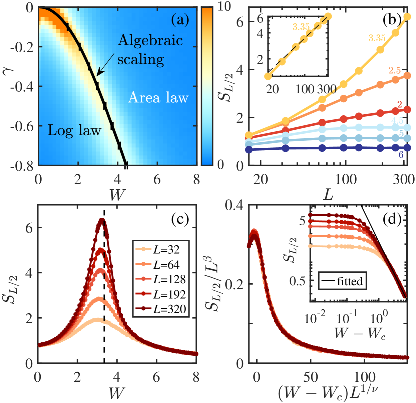
In this work, we study the dynamics of a half-filled many-body state under the evolution of the disordered Hatano-Nelson (HN) model with open boundaries. We find that the area-law scaling of the entanglement entropy in the disorder-free HN model may develop into a logarithmic scaling at small disorder, that is, $S_{L/2}\propto\log L$. As we further raise the disorder strength, the system reenters an area-law regime with the entanglement entropy being independent of the system size. At the critical point between the log-law and area-law regimes, the entanglement entropy exhibits a universal algebraic scaling with $S_{L/2}\sim L^{\beta}$ and $\beta\approx 0.5$. Based on the entanglement entropy, we map out the phase diagram of the disordered HN model including a log-law and an area-law phases with respect to the asymmetric hopping strength and the disorder strength [see Fig. 1(a)]. By examining the subsystem entanglement entropy, the connected correlation function and the mutual information, we further show that such a log-law phase does not possess a conformal invariance. Finally, we demonstrate the existence of a phase transition from the log-law to the area-law entanglement for the HN model with periodic boundaries.

Hatano-Nelson model.—To study the entanglement phase transition, we consider the paradigmatic HN model with onsite disorder described by the following Hamiltonian HN1996PRL

$$\hat{H}=\sum_{i}\left(J_{L}\hat{c}_{i}^{\dagger}\hat{c}_{i+1}+J_{R}\hat{c}_{i+1}^{\dagger}\hat{c}_{i}+m_{i}\hat{c}_{i}^{\dagger}\hat{c}_{i}\right),$$ (1)

where $\hat{c}_{i}^{\dagger}$ ($\hat{c}_{i}$) is the fermionic creation (annihilation) operator at the $i$th site, $J_{L}=-(J-\gamma)/2$ and $J_{R}=-(J+\gamma)/2$ with $J$ and $\gamma$ being real parameters depicting the strengths of symmetric and asymmetric hopping, respectively, and $m_{i}$ is the on-site disorder uniformly sampled in $[-W/2,W/2]$ with $W$ denoting the disorder strength. Without disorder ($W=0$), the Hamiltonian under open boundary conditions (OBCs) exhibits non-Hermitian skin effects when $0<|\gamma|<|J|$, with all single-particle eigenstates localized at one boundary. In the following, we will set $J=1$ as the units of energy.

To study the entanglement behavior at a sufficiently long time, we consider the following evolving state at time $t$,

$$|\psi(t)\rangle={e^{-i\hat{H}t}|\psi_{0}\rangle}/\lVert{e^{-i\hat{H}t}|\psi_{0}\rangle}\rVert,$$ (2)

where $|\psi_{0}\rangle$ is a many-body state with $L/2$ fermions for a system with $L$ sites ($L$ is even). We consider the Néel state $|\psi_{0}\rangle=\prod_{j=1}^{L/2}\hat{c}_{2j}^{\dagger}|0\rangle$ as an initial state with $|0\rangle$ denoting the vacuum state. We note that the dynamics described by Eq. (2) can be realized in an open quantum system by post-selecting a quantum trajectory where no particle loss is detected Gullans2021PRL; Ryu2022arXiv. Since the Hamiltonian in Eq. (1) is quadratic and the initial state $|\psi_{0}\rangle$ is a Slater determinant state, the final state $|\psi(t)\rangle$ is also a determinant state and its correlation matrix $D_{ij}(t)=\langle\psi(t)|\hat{c}_{i}^{\dagger}\hat{c}_{j}|\psi(t)\rangle$ can be efficiently calculated (see Supplemental Material Sec. S-1 SM for details). The von Neumann entanglement entropy $S_{A}$ between a subsystem $A$ and the rest of the system can be obtained by Peschel2003JPA

$$S_{A}=-\text{Tr}[D_{A}\log D_{A}+(1-D_{A})\log(1-D_{A})],$$ (3)

where $D_{A}$ is the correlation matrix for the subsystem $A$. In the following, we consider $A=\{1,2,...,l\}$ and label $S_{A}$ as $S_{l}$. We note that all the quantities are averaged over $500$ [only for Fig. 1(a)] or $2000$ random configurations in numerical calculations.

Entanglement phase transitions under open boundary conditions.—We now study the entanglement behavior of the state $|\psi(t)\rangle$ at sufficiently long times under OBCs. For a Hermitian Hamiltonian with $\gamma=0$, the system exhibits a volume-law entanglement when $W=0$, whereas nonzero disorder immediately drives the system to an entanglement area-law phase due to the Anderson localization. For the non-Hermitian Hamiltonian without disorder, a previous study shows that the entanglement obeys an area law due to the skin effects which push all the particles towards one boundary Ryu2022arXiv. When disorder is sufficiently strong, we expect that the long-time evolution leads to a state obeying an area law since all the single-particle eigenstates are localized on single sites so that the initial state $|\psi_{0}\rangle$ stays unchanged. However, it remains unclear whether there are entanglement phase transitions between these two limiting cases.

In Fig. 1(a), we map out the phase diagram based on the entanglement entropy, illustrating the existence of entanglement phase transitions as we increase the disorder strength $W$. In fact, our numerical results (up to $L=320$) suggest that for small disorder strength $W$, the entanglement entropy $S_{L/2}$ of a half system grows logarithmically with the system size $L$, as shown in Fig. 1(b). One can find such a log-law regime in Fig. 1(a). Further increasing the disorder strength leads to an area-law entanglement, reminiscent of the Anderson localized phase in Hermitian systems. At the transition point between the log-law and area-law regimes, the entanglement entropy exhibits an algebraic scaling $S_{L/2}\propto L^{\beta}$ with $\beta\approx 0.5$ [see the inset of Fig. 1(b)]. These different scaling behaviors can also be clearly observed in Fig. 1(c), where $S_{L/2}$ grows with $L$ (stays unchanged) for small $W$ (large $W$); the algebraic scaling manifests in a peak around the phase transition point due to a faster growth of entanglement.

To further characterize the entanglement phase transition, we adopt a finite-size scaling form for $S_{L/2}$ given by Fisher2018PRB

$$S_{L/2}(W,L)=L^{\beta}F[(W-W_{c})L^{1/\nu}],$$ (4)

with $W\gtrapprox W_{c}$. For $W\gg W_{c}$, one can find that $S_{L/2}$ is independent of the system size $L$, while at $W=W_{c}$, $S_{L/2}$ scales algebraically with $L$. Therefore $F(x)$ satisfies

$$F(x)\propto\left\{\begin{aligned} \text{const}&,\ \ \ x=0\\ x^{-\nu\beta}&,\ \ \ x\rightarrow+\infty\end{aligned}\right.,$$ (5)

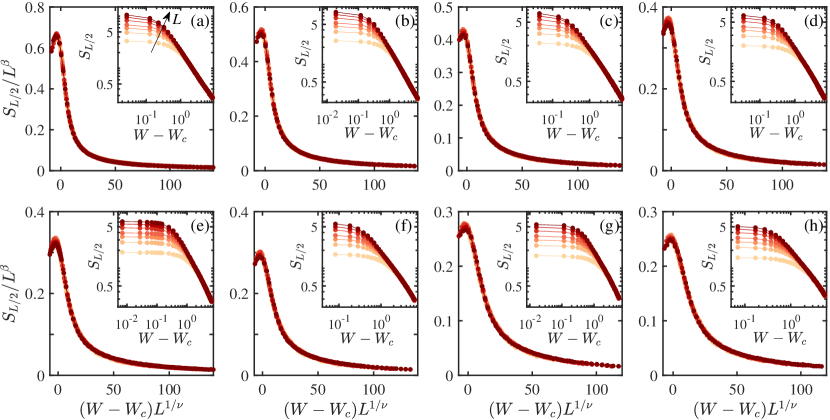
leading to $S_{L/2}(W_{c},L)\propto L^{\beta}$ at $W=W_{c}$ and $S_{L/2}(W,L)\propto(W-W_{c})^{-\nu\beta}$ for $W\geq W_{c}$. By collapsing the $S_{L/2}$ data using the scaling function Eq. (4), we obtain $W_{c}=3.35\pm 0.05$, $\beta=0.52\pm 0.03$ and $\nu=1.89\pm 0.05$; the uncertainty corresponds to the standard error of scaling results for different sets of system sizes [see Supplemental Material Sec. S-2 SM for details]. The exponents $\beta$ and $\nu$ agree well with those obtained by a direct fit as displayed in the insets of Fig. 1(b) and (d), where $\beta=0.5$ and $\beta\nu=1.09$, respectively. We also plot the scaled entanglement entropy $S_{L/2}/L^{\beta}$ as a function of $(W-W_{c})L^{1/\nu}$ for $\gamma=-0.5$ in Fig. 1(d), showing that all the data collapse to a single curve with high quality. One can also find scaling collapses for other $\gamma$ with similar exponents $\beta\approx 0.5$ and $\nu\approx 1.9$ in Supplemental Material Sec. S-2 SM.

Based on the scaling function Eq. (4), we calculate the transition points for distinct $\gamma$ and mark them out as the phase boundary in Fig. 1(a). The boundary corresponds to a large entanglement entropy due to an algebraic scaling of $S_{L/2}$ [see the region marked with bright colors in Fig. 1(a) and also the peak in Fig. 1(c)].

One may attribute the entanglement phase transition to the transition of single-particle eigenstates of the HN model from skin modes to Anderson localized states. In fact, the interplay of non-reciprocal hopping and disorder can result in partially extended single-particle eigenstates for the Hamiltonian where $\hat{H}=\sum_{i,j}[H]_{ij}\hat{c}_{i}^{\dagger}\hat{c}_{j}$ Ryu2021PRL; Chen2019PRB. To explain such a behavior, we transform $H$ to a Hermitian Hamiltonian ${H}^{\prime}={H}(J\rightarrow J^{\prime},\gamma\rightarrow 0)$ by ${H}^{\prime}=S^{-1}{H}S$, where $S=\mathrm{diag}\left\{r^{1/2},r,\dots,r^{L/2}\right\}$ with $r=|(J+\gamma)/(J-\gamma)|$ and $J^{\prime}=\text{sgn}(J)\sqrt{J^{2}-\gamma^{2}}$ for $|\gamma|<|J|$. The eigenstates of $H^{\prime}$ are exponentially localized for any non-zero disorder strength $W$, which has an asymptotic form $|u_{n}^{\prime}(x)|^{2}\sim e^{-|x-x_{n}|/\xi}$ with $x_{n}$ being the localized position and $\xi$ being the localization length. Based on the similar transformation, we obtain the density profile of the right eigenstates of $H^{\prime}$, which is given by $|u_{n}^{\text{R}}(x)|^{2}\sim r^{x}e^{-|x-x_{n}|/\xi}$. Interestingly, for $re^{1/\xi}=1$, the density quickly damps to zero as $x$ increases for $x>x_{n}$ while remains the same for $x<x_{n}$, so that the state is partially extended in the $x<x_{n}$ region. Such a behavior may account for the algebraic scaling of the entanglement entropy at the critical point, which is faster than a log-law but slower than a linear scaling.

However, due to the many-body nature, the entanglement transition point with $W_{c}\approx 3.35$ clearly deviates from the value of $W_{c}=3.56$ for the single-particle transition at zero energy in Ref. Ryu2021PRL. In Supplemental Material Sec. S-3 SM, we use all the single-particle eigenstates to calculate the orthogonality index and the mean inverse participation ratio (MIPR) and find that the entanglement transition point is very close to the the orthogonality index’s transition point and the minimum of MIPR.

Figure 2: (a) The entanglement entropy $S_{l}$ for subsystems of length $l$ and (b) the density distribution $\langle\hat{n}_{i}\rangle=\langle\psi(t)|\hat{c}_{i}^{\dagger}\hat{c}_{i}|\psi(t)\rangle$ of the state $|\psi(t)\rangle$ as a function of site $i$ for different values of disorder strength $W$. (c) The connected correlation function $C(l)$ with respect to $L/\pi\sin(l\pi/L)$ for $W\in\{0,1.5,2.5,3.35,5,6\}$. The dashed line shows a power-law fit described by $C(l)\propto[L/\pi\sin(l\pi/L)]^{-1.4}$. In (a–c), the system size $L=320$. (d) The mutual information $I_{AB}$ with respect to $W$ for different system sizes $L$. The vertical dashed line marks the phase boundary. Here, $\gamma=-0.5$.

Absence of conformal invariance.—The logarithmic scaling of the entanglement entropy usually appears in one-dimensional conformal invariant quantum systems, including gapless (critical) Hermitian systems Kitaev2003PRL; Cardy2004JSM and open systems subject to continuous monitoring Diehl2021PRL; Saito2022PRL; Pal2022arXiv. In the following, we will show that the log-law regime in the disordered HN model under OBCs cannot be characterized by conformal field theories (CFTs).

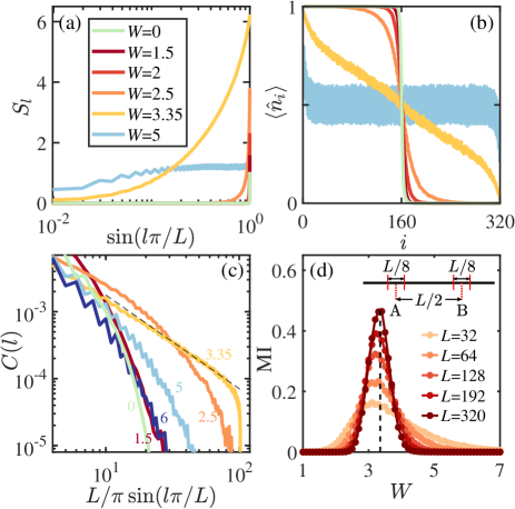
We first display the subsystem entanglement entropy $S_{l}$ in Fig. 2(a). There, we see that in the log-law regime ($W<W_{c}$), $S_{l}$ is zero for most subsystem sizes $l$ while only exhibits a sharp non-zero peak around the center of the system [$\sin(l\pi/L)=1$]. This shows a clear difference with the entanglement entropy predicted by CFTs, which is given by $S_{l}=(c/6)\log[\sin(\pi l/L)]+s_{0}$ for a finite system with open boundaries Cardy2009JPA. Such a behavior is attributable to the non-reciprocal hopping which causes a domain-wall structure in the density profile $\langle\hat{n}_{i}\rangle$ of $|\psi(t)\rangle$ as displayed in Fig. 2(b). If the subsystem $A$ (or the rest of the system) lies in the region where $\langle\hat{n}_{i}\rangle\approx 0$ or $1$, then we have $S_{A}\approx 0$ due to the fact that $\rho_{A}$ is approximately a pure state. The filled or empty region shrinks as $W$ increases and finally disappears at the critical point, leading to a nonzero $S_{l}$ for any $l$ at $W=W_{c}$. When $W>W_{c}$, $S_{l}$ exhibits an area-law behavior [see the cyan line in Fig. 2(a)].

In addition, we perform numerical calculations of the connected density-density correlation function defined as

$$C(l)=\langle\hat{n}_{L/2}\rangle\langle\hat{n}_{L/2+l}\rangle-\langle\hat{n}_{L/2}\hat{n}_{L/2+l}\rangle.$$ (6)

For the determinant state $|\psi(t)\rangle$, we have $C(l)=|\langle\hat{c}_{L/2}^{\dagger}\hat{c}_{L/2+l}\rangle|^{2}$. Figure 2(c) shows that the correlation $C(l)$ exhibits an exponential decay for all $W$ except at the critical point, in stark contrast to that of conformal invariant systems where $C(l)\sim l^{-2}$ Peschel2004JSM; Lucas2020PRR; Diehl2021PRL; Pal2022arXiv. At the critical point $W=W_{c}$, $C(l)$ decays algebraically as $C(l)\sim l^{-1.4}$.

We further calculate the mutual information $I_{AB}=S_{A}+S_{B}-S_{A\cup B}$ between two disjointed subsystems $A$ and $B$, which can serve as another indicator for conformal symmetry Fisher2019PRB; Diehl2021PRL; Yao2022PRL. Figure 2(d) shows that in both the log-law and area-law regimes, $I_{AB}$ approaches zero as $L$ increases, in contrast to a conformal invariant case where the mutual information features a nonzero and constant value for fixed subsystems $A$ and $B$ [e.g., see the inset of Fig. 2(d)] Cardy2009JPA. In the log-law regime, this may be caused by the fact that both $A$ and $B$ lies in the region where $\langle\hat{n}_{i}\rangle=0$ or $1$. Intriguingly, we also find that the mutual information grows with $L$ at the critical point.

Figure 3: (a) The linear-log plot of the entanglement entropy $S_{L/2}$ versus the system size $L$ for $W\in\{1.5,2,2.5,3.4,4.5,5,6\}$. The inset shows $S_{L/2}$ for $W=3.4$ with $L$ up to $1024$, where the black solid line is a guide for eyes. (b) The entanglement entropy $S_{L/2}$ as a function of the disorder strength $W$ for various $L$. (c) The connected correlation function $C(l)$ with respect to $L/\pi\sin(l\pi/L)$ for systems with $L=600$ . The dashed lines are power-law fits $C(l)\propto[L/\pi\sin(l\pi/L)]^{-\alpha}$ with $\alpha=1.75$, $1.81$ and $1.46$ for $W=1.5$, $2.5$ and $3.4$, respectively. We also plot a grey line corresponding to $\alpha=2$ for a visual guide. (d) The mutual information $I_{AB}$ versus the disorder strength $W$. The inset displays the $I_{AB}$ as a function of the system size. The vertical dashed lines in (b) and (d) correspond to $W=3.4$.

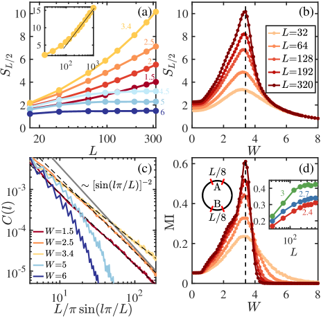
Entanglement phase transitions under periodic boundary conditions.—Next, we study the entanglement properties of the HN model under periodic boundary conditions (PBCs). Without disorder, we have proved that the entanglement entropy of $|\psi(t)\rangle$ at long times scales logarithmically with the system size as $S_{L/2}=(1/3)\log L$ (see Supplemental Material Sec. S-4 SM for the proof). As the disorder strength $W$ increases, the sub-extensive entanglement growth will be destroyed due to the Anderson localization, giving rise to a similar log-to-area-law entanglement phase transition [see Fig. 3(a) and (b)]. However, in stark contrast to the OBC case where $S_{L/2}$ scales algebraically at the critical point, we find that the entanglement entropy around the critical point tends to converge to a logarithmic scaling under PBCs [see the inset of Fig. 3(a)].

We further calculate the connected correlation function $C(l)$ under PBCs. Figure 3(c) illustrates that in the full log-law regime, the correlation $C(l)$ exhibits an algebraic scaling with $L/\pi\sin(l\pi/L)$, that is, $C(l)\propto[L/\pi\sin(l\pi/L)]^{-\alpha}$. The power-law fits in Fig. 3(c) suggest that the exponent $\alpha<2$ for finite $W$, in contrast to the case for $W=0$ where $\alpha=2$ (see Supplemental Material Sec. S-4 SM for derivation). For larger $W$, $C(l)$ displays an exponential decay in agreement with the area-law behavior of the entanglement entropy. To further diagnose the conformal invariance, we calculate the mutual information $I_{AB}$. Figure 3(d) shows that in the log-law regime, the mutual information tends to approach constant values for large systems. However, at the critical point, it exhibits a clear increase as we increase the system size, and in the area-law regime, it decreases to zero, similar to the OBC case. Our numerical results thus suggest that the conformal invariance would be preserved in the log-law regime except at the critical point.

In summary, we have studied the dynamics of a half-filled many-body state of free fermions in the HN model and found the existence of entanglement phase transitions under both OBCs and PBCs. For OBCs, although the entanglement entropy obeys the area-law scaling in the case without disorder, our numerical results suggest that the area-law scaling may develop into a logarithmic scaling in the presence of small disorder. We further show that the entanglement entropy undergoes a phase transition into an area-law when the disorder becomes sufficiently large. At the critical point, the entanglement features an algebraic scaling $S_{L/2}\sim L^{\beta}$ with $\beta\approx 0.5$. Our numerical results also show that the log-law regime under PBCs preserves the conformal invariance while under OBCs it loses the conformal invariance. We also want to remark that our results are not restricted to the HN model and can be found in other non-Hermitian systems with skin effects, such as the non-Hermitian Su-Schrieffer-Heeger model TonyLee; Yao2018PRL1. While postselection is required to achieve the non-Hermitian evolution in Eq. (2), it has recently been shown that measurements can induce skin effects in monitored systems, where the trajectory averaged entanglement entropy obeys an area-law scaling ChenFang2022arXiv; ShuChen2022arXiv. We thus expect that disorder can drive a similar entanglement phase transition in these systems where postselection is not required. Our results demonstrate that the interplay between non-Hermitian skin effects and disorder leads to a novel class of entanglement phase transitions, thereby opening an avenue for exploring entanglement phase transitions in disordered non-Hermitian systems with skin effects.

Supplemental Material for Entanglement Phase Transitions in Disordered Non-Hermitian Systems Kai Li These authors contribute equally to this work. Ze-Chuan Liu These authors contribute equally to this work. Yong Xu

I Supplemental Material

In the Supplemental Material, we will elaborate on how to calculate the entanglement entropy in Section S-1, provide more details about the scaling collapse of the entanglement entropy in Section S-2, present the orthogonality index and mean inverse participation ratio in Section S-3, and finally prove that the long-time entanglement entropy for the pristine HN model under PBCs obeys a logarithmic scaling in Section S-4.

II S-1. Details on how to calculate the entanglement entropy

In this section, we will elaborate on how to calculate the dynamics of the entanglement entropy (also see Ref. Ryu2022arXiv2). We consider an initial determinant state $|\psi_{0}\rangle$ evolved by a non-Hermitian free fermion Hamiltonian $\hat{H}=\sum_{ij}H_{ij}\hat{c}_{i}^{\dagger}\hat{c}_{j}$. The dynamics is governed by

$$|\psi(t)\rangle=\frac{e^{-i\hat{H}t}|\psi_{0}\rangle}{\sqrt{\langle\psi_{0}|e^{i\hat{H}^{\dagger}t}e^{-i\hat{H}t}|\psi_{0}\rangle}}.$$ (S1)

Without loss of generality, we choose the Néel state as an initial state, that is, $|\psi_{0}\rangle=\prod_{i=1}^{L/2}\hat{c}_{2i}^{\dagger}|0\rangle$. Then, the evolving state $|\psi(t)\rangle$ at time $t$ can be written as

$$|\psi(t)\rangle =\frac{1}{\sqrt{N(t)}}e^{-i\hat{H}t}\prod_{i=1}^{L/2}\hat{c}_{2i}^{\dagger}|0\rangle=\frac{1}{\sqrt{N(t)}}\prod_{i=1}^{L/2}\hat{c}_{2i}^{\dagger}(t)e^{-i\hat{H}t}|0\rangle$$ (S2)

$$=\frac{1}{\sqrt{N(t)}}\prod_{i=1}^{L/2}\hat{c}_{2i}^{\dagger}(t)|0\rangle,$$

where $N(t)=\langle\psi_{0}|e^{i\hat{H}^{\dagger}t}e^{-i\hat{H}t}|\psi_{0}\rangle$ and $\hat{c}_{i}^{\dagger}(t)=e^{-i\hat{H}t}\hat{c}_{i}^{\dagger}e^{i\hat{H}t}=\sum_{j=1}^{L}[e^{-iHt}]_{ji}\hat{c}_{j}^{\dagger}$. We see that $|\psi(t)\rangle$ is also a determinant state except that the operators $\hat{c}_{2i}^{\dagger}(t)$ are not necessarily orthogonal. We can write the unnormalized evolving state as

$$|\tilde{\psi}(t)\rangle=\prod_{i=1}^{L/2}\hat{c}_{2i}^{\dagger}(t)|0\rangle=\left[\prod\nolimits_{j=1}^{L/2}\left(\sum\nolimits_{i=1}^{L}[U(t)]_{ij}\hat{c}_{i}^{\dagger}\right)\right]|0\rangle,$$ (S3)

where

$$U(t)=e^{-iHt}U_{0}$$ (S4)

with $U_{0}$ (an $L\times\frac{L}{2}$ matrix) being a collection of all the initial single-particle states with $[U_{0}]_{ij}=\delta_{i,2j}$.

We now apply a QR decomposition on $U(t)$ and obtain $U(t)=QR$, where $Q$ is an $L\times\frac{L}{2}$ matrix satisfying $Q^{\dagger}Q=1$ and $R$ is an upper-triangular matrix. Substituting the decomposition into Eq. (S3) yields

$$|\tilde{\psi}(t)\rangle=\left[\prod\nolimits_{j=1}^{L/2}\left(\sum\nolimits_{k=1}^{L/2}R_{kj}\sum\nolimits_{i=1}^{L}Q_{ik}\hat{c}_{i}^{\dagger}\right)\right]|0\rangle.$$ (S5)

Let us define $\hat{\gamma}_{k}^{\dagger}=\sum_{i=1}^{L}Q_{ik}\hat{c}_{i}^{\dagger}$. They are fermionic creation operators because they satisfy the anti-commutation relations, i.e., $\{\gamma_{i}^{\dagger},\gamma_{j}^{\dagger}\}=0$ and $\{\gamma_{i},\gamma_{j}^{\dagger}\}=\delta_{ij}$. It follows that the unnormalized evolving states can be written in terms of these new operators as

$$|\tilde{\psi}(t)\rangle =\left[\prod\nolimits_{j=1}^{L/2}\left(\sum\nolimits_{k=1}^{L/2}R_{kj}\gamma_{k}^{\dagger}\right)\right]|0\rangle$$ (S6)

$$=(R_{1,\frac{L}{2}}\gamma_{1}^{\dagger}+\cdots+R_{\frac{L}{2},\frac{L}{2}}\gamma_{\frac{L}{2}}^{\dagger})\cdots(R_{13}\gamma_{1}^{\dagger}+R_{23}\gamma_{2}^{\dagger}+R_{33}\gamma_{3}^{\dagger})(R_{12}\gamma_{1}^{\dagger}+R_{22}\gamma_{2}^{\dagger})(R_{11}\gamma_{1}^{\dagger})|0\rangle$$

$$=(R_{\frac{L}{2},\frac{L}{2}}\gamma_{\frac{L}{2}}^{\dagger})\cdots(R_{33}\gamma_{3}^{\dagger})(R_{22}\gamma_{2}^{\dagger})(R_{11}\gamma_{1}^{\dagger})|0\rangle$$

$$=\left(\prod\nolimits_{i=1}^{L/2}R_{ii}\gamma_{i}^{\dagger}\right)|0\rangle.$$

Since $\langle\tilde{\psi}(t)|\tilde{\psi}(t)\rangle=(\prod_{i=1}^{L/2}R_{ii})^{2}$, we arrive at

$$|\psi(t)\rangle=\prod\nolimits_{i=1}^{L/2}\gamma_{i}^{\dagger}|0\rangle.$$ (S7)

The correlation function of the final state, defined as $D_{ij}(t)=\langle\psi(t)|\hat{c}_{i}^{\dagger}\hat{c}_{j}|\psi(t)\rangle$, can be easily calculated by

$$D(t)=(QQ^{\dagger})^{T}.$$ (S8)

We then can evaluate the von Neumann entanglement entropy $S_{A}$ between a subsystem $A$ and the rest of the system by Peschel2003JPA2

$$S_{A}=-\text{Tr}[D_{A}\log D_{A}+(1-D_{A})\log(1-D_{A})],$$ (S9)

where $D_{A}$ denotes the correlation matrix for the subsystem $A$.

In principle, one can perform a single QR decomposition to obtain the correlation function $D(t)$ even if $t$ is large. However, since the Hamiltonian is non-Hermitian, the elements in $U(t)$ may grow or decay exponentially with $t$. To avoid numerical instabilities, we perform a QR decomposition for every time step $\Delta t$, i.e.,

$$U(t+\Delta t)=\text{qr}[e^{-iH\Delta t}U(t)],$$ (S10)

where qr stands for the QR decomposition.

In our numerical calculations, we set $\Delta t=2$ and $N_{t}=1000$ ($N_{t}$ denotes the number of time steps). For all the quantities in the main text, we average over the last $100$ time steps as well as $500$ or $2000$ disorder realizations. The time evolution is numerically simulated by using the matrix exponential function “expm” in a MATLAB program. In the simulation, we use $[U_{0}]_{ij}=\delta_{i,2j}$ and $\gamma<0$. Here we note that for $\gamma>0$ the numerical results for OBCs may be incorrect when the system size is large. The error might arise from the skin effect which tends to make the columns of $U(t)$ similar to each other and hard to be orthogonalized. We have checked the correctness of our results up to $L=320$ by increasing the numerical precision using MATLAB’s vpa function.

III S-2. Details on the scaling collapse of the entanglement entropy

In this section, we will provide more details about the scaling collapse of the entanglement entropy. We use Eq. (4) in the main text to perform finite-size scaling, which can be rewritten as

$$S_{L/2}(W,L)/L^{\beta}=F[(W-W_{c})L^{1/\nu}].$$ (S11)

Let us define $y(x,L)=S_{L/2}(W,L)/L^{\beta}$ where $x=(W-W_{c})L^{1/\nu}$. One needs to find an optimal set of parameters $\{W_{c},\nu,\beta\}$ such that $y(x,L)$ versus $x$ lines for different $L$ collapse to a single curve. This can be done by minimizing the loss function defined as

$$\mathcal{L}=\sum_{x,L}[y(x,L)-\bar{y}(x)]^{2},$$ (S12)

where $\bar{y}(x)=\sum_{L}y(x,L)/N_{L}$ with $N_{L}$ denoting the number of $L$ over the sum. We use the fminsearch function in a MATLAB program to find the optimal parameters that minimize $\mathcal{L}$. To estimate the uncertainty of the parameters, we extract the parameters for different sets of system sizes and evaluate the standard deviation. The data collapse and the extracted parameters are shown in Fig. S1 and Table 1, respectively.

Figure S1: (a–h) The scaling collapses of the entanglement entropy for $\gamma=-0.1,-0.2,-0.3,-0.4,-0.5,-0.6,-0.7,-0.8$. Here the system size $L\in\{32,64,96,128,192,256,320\}$ and we use brighter (deeper) colors to denote smaller (larger) system sizes. The insets show $S_{L/2}$ versus $W-W_{c}$ in a log-log scale.

Table 1: Parameters extracted by minimizing the loss function Eq. (S12) for different $\gamma$.

$\gamma$	$-0.1$	$-0.2$	$-0.3$	$-0.4$	$-0.5$	$-0.6$	$-0.7$	$-0.8$
$W_{c}$	$1.47\pm 0.01$	$2.08\pm 0.02$	$2.56\pm 0.02$	$2.97\pm 0.04$	$3.35\pm 0.05$	$3.72\pm 0.05$	$4.08\pm 0.05$	$4.43\pm 0.06$
$\nu$	$1.99\pm 0.04$	$1.91\pm 0.05$	$1.88\pm 0.05$	$1.88\pm 0.06$	$1.89\pm 0.05$	$1.89\pm 0.04$	$1.89\pm 0.03$	$1.90\pm 0.03$
$\beta$	$0.51\pm 0.01$	$0.50\pm 0.02$	$0.51\pm 0.02$	$0.51\pm 0.03$	$0.52\pm 0.03$	$0.52\pm 0.02$	$0.53\pm 0.02$	$0.53\pm 0.02$

IV S-3. Orthogonality index and mean inverse participation ratio

In the main text, we have argued that the entanglement phase transition for a hall-filled many-body state may be related to the single-particle phase transition from skin states to Anderson localized states. In this section, we will show that the entanglement phase transition point is very close to the transition point of the orthogonality index and the minimum of the mean inverse participation ratio (MIPR) calculated using all the single-particle eigenstates.

Since the skin states are almost linearly dependent, we thus introduce the orthogonality index defined as $O=|\det(U)|^{1/L}$ to characterize the phase transition from skin states to Anderson localized ones. Here, $U=(|u_{1}^{\text{R}}\rangle,...,|u_{L}^{\text{R}}\rangle)$ with $|u_{n}^{\text{R}}\rangle$ ($n=1,\dots,L$) being the normalized right eigenstates of the Hamiltonian. The index $O$ characterizes the degree of orthogonality for the set of all eigenstates $\{|u_{n}^{\text{R}}\rangle\}_{n=1}^{L}$. If $O=1$, the eigenstates are orthogonal; if $O<1$, they are non-orthogonal. Specifically, $O$ approaches zero if the set of eigenstates are almost linearly dependent, which is the case for a set of skin states.

Figure S2: (a) The orthogonality index $O$ and (b) the MIPR as a function of disorder strength $W$ for various system sizes. The vertical dashed lines in (a) and (b) mark the entanglement phase transition point $W_{c}=3.35$. Here, $\gamma=-0.5$.

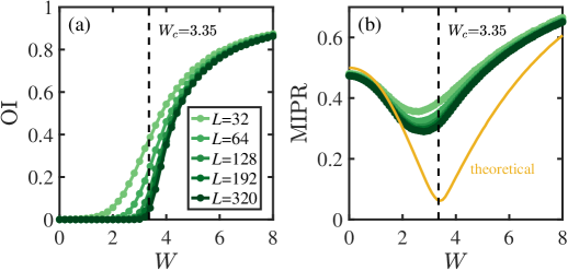
Figure S2(a) displays the orthogonality index $O$ for $\gamma=-0.5$. We see the existence of two phases: one with vanishingly small values of $O$ and the other with finite values. The phase transition from skin states to Anderson localized states is revealed by a sharp rise of $O$ from nearly zero to non-zero values for large $L$. Although we cannot identify the transition point exactly due to finite-size effects, the results indicate that the transition point is very close to the entanglement phase transition point at $W_{c}=3.35$.

We further employ the MIPR to characterize the phase transition. The MIPR is defined as $I_{\text{M}}=(\sum_{n}I_{n})/L$ where $I_{n}=\sum_{x}|u_{n}^{\text{R}}(x)|^{4}$ is the inverse participation ratio (IPR) for a normalized right eigenstate $u_{n}^{\text{R}}(x)$. When all the states are extended, the MIPR is small, approaching zero as the system size increases, whereas when all the states are localized at one site, $I_{m}=1$. Fig. S2(b) illustrates that the MIPR for the disordered HN model is large when $W$ is either small or large, consistent with the fact that both skin states and Anderson localized states are spatially localized.

Interestingly, the MIPR decays to a minimum for some disorder strength $W$ as shown in Fig. S2(b) (the existence of a minimum in the MIPR has also been found in a non-Hermitian quasicrystal Chen2019PRB2). As shown in the main text, the density distribution of $u_{n}^{\text{R}}(x)$ has an asymptotic form given by

$$|u_{n}^{\text{R}}(x)|^{2}\sim r^{x}e^{-|x-x_{n}|/\xi}=\left\{\begin{aligned} &e^{-x_{n}/\xi}\,(re^{1/\xi})^{x},\ \ \ x<x_{n}\\ &e^{x_{n}/\xi}\,(re^{-1/\xi})^{x},\ \ \ x>x_{n}\end{aligned}\right.$$ (S13)

which will exhibit different behaviors for different values of the localization length $\xi$. We assume that $\gamma<0$ so that $re^{-1/\xi}<1$, which means that the density for the $x>x_{n}$ part is always suppressed as $x$ increases. For $re^{1/\xi}<1$, the density will get enhanced as $x$ decreases for $x<x_{n}$, so that the transformed state is a skin state localized at the left boundary. While for $re^{-1/\xi}>1$, the state is exponentially localized at $x_{n}$, giving rise to an Anderson localized state. For $re^{-1/\xi}=1$, as also mentioned in the main text, the density remains the same for $x<x_{n}$ while quickly damps to zero as $x$ decreases for $x>x_{n}$, rendering the state partially extended in the region $x<x_{n}$. Thus, the states become more extended as $W$ approaches the phase transition point, accounting for the fact that the MIPR reaches a minimum around the critical point.

To eliminate the finite-size effects, we further calculate the MIPR based on

$$I_{\text{M}}=\int dED(E)I[\xi(E)]/\int dED(E),$$ (S14)

where $\int dE$ denotes an integral over energy $E$, $D(E)$ is the density of state of the similar transformed Hamiltonian $H^{\prime}$, and $I[\xi(E)]$ is the IPR computed based on the asymptotic form Eq. (S13) at energy $E$, with the localization length $\xi(E)$ determined by the transfer matrix method Kramer1983ZPB. Fig. S2(b) plots the calculated MIPR [see the yellow line in Fig. S2(b)], showing the existence of a dip around $W=3.4$, which is very close to the critical point $W_{c}=3.35$ for the entanglement phase transition.

V S-4. Long-time entanglement entropy for the pristine HN model under PBCs

In this section, we will show that the long-time entanglement entropy for the HN model under PBCs without disorder obeys a logarithmic scaling. We first prove that the system will converge to a state with the largest imaginary eigenenergy under the evolution of a non-Hermitian Hamiltonian.

We denote the many-body eigenenergy in the $N$-particle subspace as $E_{n}=\varepsilon_{n}^{\text{R}}+i\varepsilon_{n}^{\text{I}}$ and the corresponding right (left) eigenstate as $|\phi_{n}^{R}\rangle$ ($\langle\phi_{n}^{L}|$). Given an initial $N$-particle determinant state $|\psi_{0}\rangle$, the evolving state $|\psi(t)\rangle$ can be written as

$$|\psi(t)\rangle =\frac{\sum_{n}e^{-i\varepsilon_{n}^{\text{R}}t}e^{\varepsilon_{n}^{\text{I}}t}|\phi_{n}^{R}\rangle\langle\phi_{n}^{L}|\psi_{0}\rangle}{\sqrt{\langle\psi_{0}|e^{i\hat{H}^{\dagger}t}e^{-i\hat{H}t}|\psi_{0}\rangle}}$$ (S15)

$$=\frac{e^{\varepsilon_{1}^{\text{I}}t}}{\sqrt{\langle\psi_{0}|e^{i\hat{H}^{\dagger}t}e^{-i\hat{H}t}|\psi_{0}\rangle}}\sum_{n}e^{-i\varepsilon_{n}^{\text{R}}t}e^{(\varepsilon_{n}^{\text{I}}-\varepsilon_{1}^{\text{I}})t}|\phi_{n}^{R}\rangle\langle\phi_{n}^{L}|\psi_{0}\rangle.$$

By assuming $\varepsilon_{1}^{\text{I}}>\varepsilon_{2}^{\text{I}}>\dots$, one can find that $|\psi(+\infty)\rangle=|\phi_{1}^{R}\rangle$ up to a phase factor. Therefore, the entanglement entropy at long times is the same as that of the many-body eigenstate with the largest imaginary eigenenergy, if only a single eigenstate has the largest imaginary eigenenergy. Otherwise, the final state will become a superposition of the eigenstates with the largest imaginary eigenenergy.

For the HN model without disorder under PBCs, the single-particle eigenstates are given by $|k\rangle=\hat{c}_{k}^{\dagger}|0\rangle=\frac{1}{\sqrt{L}}\sum_{j}e^{ikj}\hat{c}_{j}^{\dagger}|0\rangle$ corresponding to eigenenergies $E_{k}=-J\cos k+i\gamma\sin k$ where $k=k_{n}=2\pi n/L$ with $n=-L/2,-L/2+1,...,L/2-1$. Without loss of generality, we will consider the case with $\gamma<0$ in the following. Starting from an initially half-filled state, the system will converge to a superposition of $|\Psi_{1}\rangle=\prod_{n=-L/2}^{-1}\hat{c}_{k_{n}}^{\dagger}|0\rangle$ and $|\Psi_{2}\rangle=\prod_{n=-L/2+1}^{0}\hat{c}_{k_{n}}^{\dagger}|0\rangle$, which are many-body eigenstates with the largest imaginary eigenenergy in the half-filled subspace. For infinitely large $L$, the final state is a Slater determinant of all the Bloch states with momentum $k\in[-\pi,0]$, whose correlation matrix is given by

$$D_{mn}=\int_{-\pi}^{0}\frac{dk}{2\pi}e^{-ik(m-n)}=\frac{i}{2\pi}\frac{1-e^{i\pi(m-n)}}{m-n}.$$ (S16)

When $m-n$ is even, $D_{mn}=0$; otherwise, $D_{mn}=i/[\pi(m-n)]$ so that $|D_{mn}|^{2}=1/[\pi^{2}(m-n)^{2}]$, indicating that the density-density correlation function $C(l)\propto 1/l^{2}$. The entanglement entropy is determined by the eigenvalues of $D_{A}$ with $[D_{A}]_{mn}=D_{mn}$ for $m,n\in A$.

To evaluate the entanglement entropy given by $D_{A}$, we consider the ground state of a Hermitian free fermion chain with Hamiltonian $\hat{H}_{h}=-\sum_{j}(\hat{c}_{j}^{\dagger}\hat{c}_{j+1}+\text{H.c.})$. Since the ground state of $\hat{H}_{h}$ is a Slater determinant of Bloch states with momentum $k\in[-\pi/2,\pi/2]$, its correlation matrix is given by

$$D_{mn}^{\prime}=\int_{-\pi/2}^{\pi/2}\frac{dk}{2\pi}e^{-ik(m-n)}=\frac{\sin[\pi(m-n)/2]}{\pi(m-n)},$$ (S17)

which is related to $D$ by a unitary transformation $D^{\prime}=U^{\dagger}DU$ with $U=\text{diag}\{i,i^{2},i^{3},...\}$ (similar property holds for $D_{A}$ and $D_{A}^{\prime}$). Based on a continuum approximation, it has been proved that the entanglement entropy of the ground state of $\hat{H}_{h}$ is asymptotically given by $S=\frac{1}{3}\ln L$ at large $L$ Peschel2004JSM2; Peschel2009JPA. We thus conclude that the long-time entanglement entropy for the HN model under PBCs is also given by $S=\frac{1}{3}\ln L$ for sufficiently large $L$, owing to the fact that $D_{A}$ and $D_{A}^{\prime}$ share the same eigenvalues. We have also numerically checked that the entanglement entropy is actually described by $S=k\ln L+b$ with $k$ being exactly $1/3$ and $b\approx 0.34$. The non-zero intercept $b$ is attributed to the fact that the derivation for the eigenvalues of $D_{A}^{\prime}$ requires a continuum approximation Peschel2004JSM2, which is not valid for small $L$.

References

- (1) K. Kawabata, T. Numasawa, and S. Ryu, Phys. Rev. X 13, 021007 (2023).
- (2) I. Peschel, J. Phys. A 36, L205 (2003).
- (3) H. Jiang, L.-J. Lang, C. Yang, S.-L. Zhu, and S. Chen, Phys. Rev. B 100, 054301 (2019).
- (4) A. MacKinnon and B. Kramer, Z. Phys. B 53, 1 (1983).
- (5) I. Peschel, J. Stat. Mech. (2004) P06004.
- (6) I. Peschel and V. Eisler, J. Phys. A 42, 504003 (2009).