When are ensembles really effective?

Abstract

Ensembling has a long history in statistical data analysis, with many impactful applications. However, in many modern machine learning settings, the benefits of ensembling are less ubiquitous and less obvious. We study, both theoretically and empirically, the fundamental question of when ensembling yields significant performance improvements in classification tasks. Theoretically, we prove new results relating the ensemble improvement rate (a measure of how much ensembling decreases the error rate versus a single model, on a relative scale) to the disagreement-error ratio. We show that ensembling improves performance significantly whenever the disagreement rate is large relative to the average error rate; and that, conversely, one classifier is often enough whenever the disagreement rate is low relative to the average error rate. On the way to proving these results, we derive, under a mild condition called competence, improved upper and lower bounds on the average test error rate of the majority vote classifier. To complement this theory, we study ensembling empirically in a variety of settings, verifying the predictions made by our theory, and identifying practical scenarios where ensembling does and does not result in large performance improvements. Perhaps most notably, we demonstrate a distinct difference in behavior between interpolating models (popular in current practice) and non-interpolating models (such as tree-based methods, where ensembling is popular), demonstrating that ensembling helps considerably more in the latter case than in the former.

1 Introduction

The fundamental ideas underlying ensemble methods can be traced back at least two centuries, with Condorcet’s Jury Theorem among its earliest developments [Con85]. This result asserts that if each juror on a jury makes a correct decision independently and with the same probability $p>1/2$, then the majority decision of the jury is more likely to be correct with each additional juror. The general principle of aggregating knowledge across imperfectly correlated sources is intuitive, and it has motivated many ensemble methods used in modern statistics and machine learning practice. Among these, tree-based methods like random forests [Bre01] and XGBoost [CG16] are some of the most effective and widely-used.

With the growing popularity of deep learning, a number of approaches have been proposed for ensembling neural networks. Perhaps the simplest of them are so-called deep ensembles, which are ensembles of neural networks trained from independent initializations [ABP⁺22, ABPC22, FHL19]. In some cases, it has been claimed that such deep ensembles provide significant improvement in performance [FHL19, OFR⁺19, ALMV20]. Such ensembles have also been used to obtain uncertainty estimates for prediction [LPB17] and to provide more robust predictions under distributional shift. However, the benefits of deep ensembling are not universally accepted. Indeed, other works have found that ensembling is less necessary for larger models, and that in some cases a single larger model can perform as well as an ensemble of smaller models [HVD⁺15, BCNM06, GJS⁺20, ABP⁺22]. Similarly mixed results, where empirical performance does not conform with intuitions and popular theoretical expectations, have been reported in the Bayesian approach to deep learning [INLW21]. Furthermore, an often-cited practical issue with ensembling, especially of large neural networks, is the constraint of storing and performing inference with many distinct models.

In light of the increase in computational cost, it is of great value to understand exactly when we might expect ensembling to improve performance non-trivially. In particular, consider the following practical scenario: a practitioner has trained a single (perhaps large and expensive) model, and would like to know whether they can expect significant gains in performance from training additional models and ensembling them. This question lacks a sufficient answer, both from the theoretical and empirical perspectives, and hence motivates the main question of the present work:

The present work addresses this question, both theoretically and empirically, under very general conditions. We focus our study on the most popular ensemble classifier—the majority vote classifier (Definition 1), which we denote by $h_{\mathrm{MV}}$—although our framework also covers variants such weighted majority vote methods.

Theoretical results.

Our main theoretical contributions, contained in Section 3, are as follows. First, we formally define the ensemble improvement rate ($\mathrm{EIR}$, Definition 3), which measures the decrease in error rate from ensembling, on a relative scale. We then introduce a new condition called competence (Assumption 1) that rules out pathological cases, allowing us to prove stronger bounds on the ensemble improvement rate. Specifically, 1) we prove (in Theorem 1) that competent ensembles can never hurt performance, and 2) we prove (in Theorem 2) that the $\mathrm{EIR}$ can be upper and lower bounded by linear functions of the disagreement-error ratio ($\mathrm{DER}$, Definition 4). Our theoretical results predict that ensemble improvement will be high whenever disagreement is large relative to the average error rate (i.e., $\mathrm{DER}>1$). Moreover, we show (in Appendix A.3) that as Corollaries of our theoretical results, we obtain new bounds on the error rate of the majority vote classifier that significantly improve on previous results, provided the competence assumption is satisfied.

Empirical results.

In light of our new theoretical understanding of ensembling, we perform a detailed empirical analysis of ensembling in practice. In Section 4, we evaluate the assumptions and predictions made by the theory presented in Section 3. In particular, we verify on a variety of tasks that the competence condition holds, we verify empirically the linear relationship between the $\mathrm{EIR}$ and the $\mathrm{DER}$, as predicted by our bounds, and we suggest directions through which our theoretical results might be improved. In Section 5, we provide significant evidence for distinct behavior arising for ensembles in and out of the “interpolating regime,” i.e., when each of the constituent classifiers in an ensemble has sufficient capacity to achieve zero training error. We show 1) that interpolating ensembles exhibit consistently lower ensemble improvement rates, and 2) that this corresponds to ensembles transitioning (sometimes sharply) from the regime $\mathrm{DER}>1$ to $\mathrm{DER}<1$. Finally, we also show that tree-based ensembles represent a unique exception to this phenomenon, making them particularly well-suited to ensembling.

In addition to the results presented in the main text, we provide supplemental theoretical results (including all proofs) in Appendix A, as well as supplemental empirical results in Appendix B.

2 Background and preliminaries

In this section, we present some background as well as preliminary results of independent interest that set the context for our main theoretical and empirical results.

2.1 Setup

In this work, we focus on the $K$-class classification setting, wherein the data $(X,Y)\in\mathcal{X}\times\mathcal{Y}\sim\mathcal{D}$ consist of features $\bm{x}\in\mathcal{X}$ and labels $y\in\mathcal{Y}=\{1,\dots,K\}$. Classifiers are then functions $h:\mathcal{X}\to\mathcal{Y}$ that belong to some set $\mathcal{H}$. To measure the performance of a single classifier $h$ on the data distribution $\mathcal{D}$, we use the usual error rate:

$$L_{\mathcal{D}}(h)=\mathbb{E}_{X,Y\sim\mathcal{D}}[\mathbb{1}(h(X)\neq Y)].$$

For notational convenience, we drop the explicit dependence on $\mathcal{D}$ whenever it is apparent from context.

A central object in our study is a distribution $\rho$ over classifiers. Depending on the context, this distribution could represent a variety of different things. For example, $\rho$ could be:

1. A discrete distribution on a finite set of classifiers $\{h_{1},\dots,h_{M}\}$ with weights $\rho_{1},\dots,\rho_{M}$, e.g., representing normalized weights in a weighted ensembling scheme;

2. A distribution over parameters $\theta$ of a parametric family of models, $h_{\theta}$, determined, e.g., by a stochastic optimization algorithm with random initialization;

3. A Bayesian posterior distribution.

The distribution $\rho$ induces two error rates of interest. The first is the average error rate of any single classifier under $\rho$, defined to be $\mathbb{E}_{h\sim\rho}[L(h)]$. The second is the error rate of the majority vote classifier, $h_{\mathrm{MV}}$, which is defined for a distribution $\rho$ as follows.

Definition 1 (Majority vote classifier).

Given $\rho$, the majority vote classifier is the classifier which, for an input $\bm{x}$, predicts the most probable class for this input among classifiers drawn from $\rho$,

$$h_{\mathrm{MV}}(\bm{x})=\operatorname*{arg\,max}_{j}\;\mathbb{E}_{h\sim\rho}[\mathbb{1}(h(\bm{x})=j)].$$

In the Bayesian context, $\rho=\rho(h\mid X_{\text{train}},y_{\text{train}})$ is a posterior distribution over classifiers. In this case, the majority vote classifier is often called the Bayes classifier, and the error rate $L(h_{\mathrm{MV}})$ is called the Bayes error rate. In such contexts, the average error rate is often referred to as the Gibbs error rate associated with $\rho$ and $\mathcal{D}$.

Finally, we will present results in terms of the disagreement rate between classifiers drawn from a distribution $\rho$, defined as follows.

Definition 2 (Disagreement).

The disagreement rate between two classifiers $h,h^{\prime}$ is given by $D_{\mathcal{D}}(h,h^{\prime})=\mathbb{E}_{X\sim\mathcal{D}}[\mathbb{1}(h(X)\neq h^{\prime}(X))]$. The expected disagreement rate is $\mathbb{E}_{h,h^{\prime}\sim\rho}[D_{\mathcal{D}}(h,h^{\prime})]$, where $h,h^{\prime}\sim\rho$ are drawn independently.

2.2 Prior work

Ensembling theory.

Perhaps the simplest general relation between the majority vote error rate and the average error rate guarantees only that the majority vote classifier is no worse than twice the average error rate [LMRR17, MLIS20]. To see this, let $W_{\rho}\equiv W_{\rho}(X,Y)=\mathbb{E}_{h\sim\rho}[\mathbb{1}(h(X)\neq Y)]$ denote the proportion of erroneous classifiers in the ensemble for a randomly sampled input-output pair $(X,Y)\sim\mathcal{D}$, and note that $\mathbb{E}[W_{\rho}]=\mathbb{E}[L(h)]$. Then, by a “first-order” application of Markov’s inequality, we have that

$$0\leq L(h_{\mathrm{MV}})\leq\mathbb{P}(W_{\rho}\geq 1/2)\leq 2\,\mathbb{E}[W_{\rho}]=2\,\mathbb{E}_{h\sim\rho}[L(h)].$$ (1)

This bound is almost always uninformative in practice. Indeed, it may seem surprising that an ensemble classifier could perform worse than the average of its constituent classifiers, much less a factor of two worse. Nonetheless, the first-order upper bound is, in fact, tight: there exist distributions $\rho$ (over classifiers) and $\mathcal{D}$ (over data) such that the majority vote classifier is twice as erroneous as any one classifier, on average. As one might expect, however, this tends to happen only in pathological cases; we give examples of such ensembles in Appendix C.

To circumvent the shortcomings of the simple first-order bound, more recent approaches have developed bounds incorporating “second-order” information from the distribution $\rho$ [MLIS20]. One successful example of this is given by a class of results known as C-bounds [GLL⁺15, LMRR17]. The most general form of these bounds states, provided $\mathbb{E}[M_{\rho}(X,Y)]>0$, that $L(h_{\mathrm{MV}})\leq 1-\mathbb{E}[M_{\rho}(X,Y)]^{2}/\mathbb{E}[M_{\rho}^{2}(X,Y)]$, where $M_{\rho}(X,Y)=\mathbb{E}_{h\sim\rho}[\mathbb{1}(h(X)=Y)]-\max_{j\neq Y}\mathbb{E}_{h\sim\rho}[\mathbb{1}(h(X)=j)]$ is called the margin. In the binary classification case, the condition $\mathbb{E}[M_{\rho}(X,Y)]>0$ is equivalent to the assumption $\mathbb{E}_{h\sim\rho}[L(h)]<1/2$. Hence, it can be viewed as a requirement that individual classifiers are “weak learners.” The same condition is used to derive a very similar bound for random forests in [Bre01], which is then further upper bounded to obtain a more intuitive (though weaker) bound in terms of the “c/s2” ratio. Relatedly, [MLIS20] obtains a bound on the error rate of the majority-vote classifier, in the special case of binary classification, directly in terms of the disagreement rate, taking the form $4\mathbb{E}[L(h)]-2\mathbb{E}[D(h,h^{\prime})]$. We note that our theory improves this bound by factor of $2$ (see Appendix A.3). Other results obtain similar expressions, but in terms of different loss functions, e.g., cross-entropy loss [ABP⁺22, OCnM22].

Other related studies.

In addition to theoretical results, there have been a number of recent empirical studies investigating the use of ensembling. Perhaps the most closely related is [ABPC22], which shows, perhaps surprisingly, that ensembles do not benefit significantly from encouraging diversity during training. In contrast to the present work, [ABPC22] focuses on the cross entropy loss for classification (which facilitates somewhat simpler theoretical analysis), whereas we focus on the more intuitive and commonly used classification error rate. Moreover, while [ABPC22] study the ensemble improvement gap (i.e., the difference between the average loss of a single classifier and the ensemble loss), we focus on the gap in error rates on a relative scale. As we show, this provides much finer insights into ensembles improvement. To complement this, [FHL19] study ensembling from a loss landscape perspective, evaluating how different approaches to ensembling, such as deep ensembles, Bayesian ensembles, and local methods like Gaussian subspace sampling compare in function and weight space diversity. Other recent work has studied the use of ensembling to provide uncertainty estimates for prediction [LPB17], and to improve robustness to out-of-distribution data [OFR⁺19], although the ubiquity of these findings has recently been questioned in [ABP⁺22].

3 Ensemble improvement, competence, and the disagreement-error ratio

In this section, our goal is to characterize theoretically the rate at which ensembling improves performance. To do this, we first need to formalize a metric to quantify the benefit from ensembling. One natural way of measuring this improvement would be to compute the gap $\mathbb{E}_{h\sim\rho}[L(h)]-L(h_{\mathrm{MV}})$. A similar gap was the focus of [ABPC22], although in terms of the cross-entropy loss, rather than the classification error rate. However, the unnormalized gap can be misleading—in particular, it will tend to be small whenever the average error rate itself is small, thus making it impractical to compare, e.g., across tasks of varying difficulty. Instead, we work with a normalized version of the average-minus-ensemble error rate gap, where the effect of the normalization is to measure this error in a relative scale. We call this the ensemble improvement rate.

Definition 3 (Ensemble improvement rate).

Given distributions $\rho$ over classifiers and $\mathcal{D}$ over data, provided that $\mathbb{E}_{h\sim\rho}[L(h)]\neq 0$, the ensemble improvement rate (EIR) is defined as

$$\mathrm{EIR}=\frac{\mathbb{E}_{h\sim\rho}[L(h)]-L(h_{\mathrm{MV}})}{\mathbb{E}_{h\sim\rho}[L(h)]}.$$

In contrast to the unnormalized gap, the ensemble improvement rate can be large even for very easy tasks with a small average error rate. Recall the simple first-order bound on the majority-vote classifier: $L(h_{\mathrm{MV}})\leq 2\mathbb{E}[L(h)]$. Rearranging, we deduce that $\mathrm{EIR}\geq-1$. Unfortunately, in the absence of additional information, this first-order bound is in fact tight: one can construct ensembles for this $L(h_{\mathrm{MV}})=2\mathbb{E}[L(h)]$ (see Appendix C). However, this bound is inconsistent with how ensembles generally behave and practice, and indeed it tells us nothing about when ensembling can improve performance. In the subsequent sections, we derive improved bounds on the $\mathrm{EIR}$ that do.

3.1 Competent ensembles never hurt

Surprisingly, to our knowledge, there is no known characterization of the majority-vote error rate that guarantees it can be no worse than the error rate of any individual classifier, on average. Indeed, it turns out this is the result of strange behavior that can arise for particularly pathological ensembles rarely encountered in practice (see Appendix C for a more detailed discussion of this). To eliminate these cases, we introduce a mild condition that we call competence.

Assumption 1 (Competence).

Let $W_{\rho}\equiv W_{\rho}(X,Y)=\mathbb{E}_{h\sim\rho}[\mathbb{1}(h(X)\neq Y)]$. The ensemble $\rho$ is competent if for every $0\leq t\leq 1/2$,

$$\mathbb{P}(W_{\rho}\in[t,1/2))\geq\mathbb{P}(W_{\rho}\in[1/2,1-t]).$$

The competence assumption guarantees that the ensemble is not pathologically bad, and in particular it eliminates the scenarios under which the naive first-order bound (1) is tight. As we will show in Section 4, the competence condition is quite mild, and it holds broadly in practice. Our first result uses competence to improve non-trivially the naive first-order bound.

Theorem 1.

Competent ensembles never hurt performance, i.e., $\mathrm{EIR}\geq 0$.

Translated into a bound on the majority vote classifier, Theorem 1 guarantees that $L(h_{\mathrm{MV}})\leq\mathbb{E}[L(h)]$, improving on the naive first-order bound (1) by a factor of two. To the best of our knowledge, the competence condition is the first of its kind, in that it guarantees what is widely observed in practice, i.e., that ensembling cannot hurt performance. However, it is insufficient to answer the question of how much ensembling can improve performance. To address this question, we turn to a "second-order" analysis involving the disagreement rate.

3.2 Quantifying ensemble improvement with the disagreement-error ratio

Our central result in this section will be to relate the $\mathrm{EIR}$ to the ratio of the disagreement to average error rate, which we define formally below.

Definition 4 (Disagreement-error ratio).

Given the distributions $\rho$ over classifiers and $\mathcal{D}$ over data, provided that $\mathbb{E}_{h\sim\rho}[L(h)]\neq 0$, the disagreement-error ratio (DER) is defined as

$$\mathrm{DER}=\frac{\mathbb{E}_{h,h^{\prime}\sim\rho}[D(h,h^{\prime})]}{\mathbb{E}_{h\sim\rho}[L(h)]}.$$

Our next result relates the $\mathrm{EIR}$ to a linear function of the $\mathrm{DER}$.

Theorem 2.

For any competent ensemble $\rho$ of $K$-class classifiers, provided $\mathbb{E}_{h\sim\rho}[L(h)]\neq 0$, the ensemble improvement rate satisfies

$$\mathrm{DER}\geq\mathrm{EIR}\geq\frac{2(K-1)}{K}\mathrm{DER}-\frac{3K-4}{K}.$$

Note that neither Theorem 1 nor Theorem 2 is uniformly stronger. In particular, if $\mathrm{DER}<(3K-4)/(2K-2)$ then the lower bound provided in Theorem 1 will be superior to the one in Theorem 2.

Theorem 2 predicts that the $\mathrm{EIR}$ is fundamentally governed by a linear relationship with the $\mathrm{DER}$ — a result that we will verify empirically in Section 4. Importantly, we note that there are two distinct regimes in which the bounds in Theorem 2 provide non-trivial guarantees.

• $\mathbf{DER}$ small ($\mathbf{<1}$). In this case, by the trivial bound (1), $\mathrm{EIR}\leq 1$, and thus the upper bound in Theorem 2 guarantees ensemble improvement cannot be too large whenever $\mathrm{DER}<1$, that is, whenever disagreement is small relative to the average error rate.

• $\mathbf{DER}$ large ($\mathbf{>1}$). In this case, the lower bound in Theorem 2 guarantees ensemble improvement whenever disagreement is sufficiently large relative to the average error rate, in particular when $\mathrm{DER}\geq(3K-4)/(2K-2)\geq 1$.

In our empirical evaluations, we will see that these two regimes ($\mathrm{DER}>1$ and $\mathrm{DER}<1$) strongly distinguish between situations in which ensemble improvement is high, and when the benefits of ensembling are significantly less pronounced.

Moreover, Theorem 2 captures an important subtlety in the relationship between ensemble improvement and predictive diversity. In particular, while general intuition—and a significant body of prior literature, as discussed in Section 2—suggests that higher disagreement leads to high ensemble improvement, this may not be the case if the disagreement is nominally large, but small relative to the average error rate.

Remark 1 (Corollaries of Theorems 1 and 2).

Using some basic algebra, the upper and lower bounds presented in Theorems 1 and 2 can easily be translated into upper and lower bounds on the error rate of the majority vote classifier itself. For the sake of space, we defer discussion of these Corollaries to Appendix A.3, although we note that the resulting bounds constitute significant improvements on existing bounds, which we verify both analytically (when possible) and empirically.

4 Evaluating the theory

In this section, we investigate the assumptions and predictions of the theory proposed in Section 3. In particular we will show 1) that the competence assumption holds broadly in practice, across a range of architectures, ensembling methods and datasets, and 2) that the $\mathrm{EIR}$ exhibits a close linear relationship with the $\mathrm{DER}$, as predicted by Theorem 2.

Before presenting our findings, we first briefly describe the experimental settings analyzed in the remainder of the paper. Our goal is to select a sufficiently broad range of tasks and methods so as to demonstrate the generality of our conclusions.

4.1 Setup for empirical evaluations

In Table 1 we provide a brief description of our experimental setup; more extensive experimental details can be found in Appendix B.1.

Table 1: Datasets and ensembles used in empirical evaluations, where $C$ denotes the number of classes, and $M$ denotes the number of classifiers.

Datasets
Dataset	C	Reference
MNIST (5K subset)	10	[Den12]
CIFAR-10	10	[KH+09]
IMDB	2	[MDP+11]
QSAR	2	[BGCT19]
Thyroid	2	[QCHL87]
GLUE (7 tasks)	2-3	[WSM+19]

Ensembles
Base classifier	Ensembling	M	Reference
ResNet20-Swish	Bayesian Ens.	100	[IVHW21]
ResNet18	Deep Ens.	5	[KH+09]
CNN-LSTM	Bayesian Ens.	100	[IVHW21]
BERT (fine-tune)	Deep Ens.	25	[DCLT19, SYT+22]
Random Features	Bagging	30	N/A
Decision Trees	Random Forests	100	[PVG+11, Bre01]

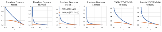
Figure 1: Verifying the competence assumption in practice. $W_{\rho}(X,Y)$ in Assumption 1 is estimated using hold-out data. Across all tasks,   $>$  , supporting Assumption 1.

4.2 Verifying competence in practice.

Our theoretical results in Section 3 relied on the competence condition. One might wonder whether competent ensembles exist, and if so how ubiquitous they are. Here, we test that assumption. (That is, we test not just the predictions of our theory, but also the assumptions of our theory.)

We have observed that the competence assumption is empirically very mild, and that in practice it applies very broadly. In Figure 1, we estimate both $\mathbb{P}(W_{\rho}\in[t,1/2))$ and $\mathbb{P}(W_{\rho}\in[1/2,1-t])$ on test data, validating that competence holds for various types of ensembles across a subset of tasks. To do this, given a test set of examples $\{(\bm{x}_{j},y_{j})\}_{j=1}^{m}$ and classifiers $h_{1},\dots,h_{N}$ drawn from $\rho$, we construct the estimator

$$\widehat{W}_{\rho}^{(j)}=\frac{1}{N}\sum_{n=1}^{N}\mathbb{1}(h_{n}(\bm{x}_{j})\neq y_{j}),$$

and we calculate $\mathbb{P}(W_{\rho}\in[t,1/2))$ and $\mathbb{P}(W_{\rho}\in[1/2,1-t])$ from the empirical CDF of $\{\widehat{W}_{\rho}^{(j)}\}_{j=1}^{m}$. In Appendix B, we provide additional examples of competence plots across more experimental settings (and we observe substantially the same results).

4.3 The linear relationship between $\mathrm{DER}$ and $\mathrm{EIR}$.

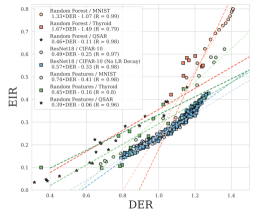
Figure 2: $\mathrm{EIR}$ is linearly correlated with the $\mathrm{DER}$. We plot the $\mathrm{EIR}$ against the $\mathrm{DER}$ across a variety of experimental settings, and we observe a close linear relationship between the $\mathrm{EIR}$ and $\mathrm{DER}$, as predicted by our theoretical results. In the legend, we also report the equation for the line of best fit within each setting, as well as the Pearson correlation.

Theorem 2 predicts a linear relationship between the $\mathrm{EIR}$ and the $\mathrm{DER}$; here we verify that this relationship holds empirically. In Figure 2, we plot the $\mathrm{EIR}$ against the $\mathrm{DER}$ across several experimental settings, varying capacity hyper-parameters (width for the ResNet18 models, number of random features for the random feature classifiers, and number of leaf nodes for the random forests), reporting the equation of the line of best fit, as well as the Pearson correlation between the two metrics. Across 6 of the 8 experimental settings evaluated, we find a very strong linear relationship – with the Pearson $R\geq 0.96$. The two exceptions are found for the Thyroid classification dataset (though there is still a strong trend between the two quantities, with $R\approx 0.8$).

Interestingly, we can compare the lines of best fit to the theoretical linear relationship predicted by Theorem 2. In the case of the binary classification datasets (QSAR and Thyroid), the bound predicts that $\mathrm{EIR}\approx\mathrm{DER}-1$; while for the 10-class problems (MNIST and CIFAR-10), the equation is $\mathrm{EIR}\approx 1.8\,\mathrm{DER}-2.6$. While for some examples (e.g., random forests on MNIST), the equations are close to those theoretically predicted, there is a clear gap between theory and the experimentally measured relationships for other tasks. In particular, we notice a significant difference in the governing equations for the same datasets between random forests and the random feature ensembles, suggesting that the relationship is to some degree modulated by the model architecture – something our theory cannot capture. We therefore see refining our theory to incorporate such information as an important direction for future work.

5 Ensemble improvement is low in the interpolating regime

In this section, we will show that the $\mathrm{DER}$ behaves qualitatively differently for interpolating versus non-interpolating ensembles, in particular exhibiting behavior associated with phase transitions. Such phase transitions are well-known in the statistical mechanics approach to learning [EdB01, MM17, TKM21, YHT⁺21], but they have been viewed as surprising from the more traditional approach to statistical learning theory [BHMM19]. We will use this to understand when ensembling is and is not effective for deep ensembles, and to explain why tree-based methods seem to benefit so much from ensembling across all settings. We say that a model is interpolating if it achieves exactly zero training error, and we say that it is non-interpolating otherwise; we call an ensemble interpolating if each of its constituent classifiers is interpolating. Note that for methods that involve resampling of the training data (e.g., bagging methods), we define the training error as the “in-bag” training, i.e., the error evaluated only on the points a classifier was trained on.

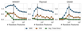
Figure 3: Bagged random feature classifiers. Blacked dashed line represents the interpolation threshold. Across all tasks, $\mathrm{DER}$ and $\mathrm{EIR}$ are maximized at this point, and then decrease thereafter.

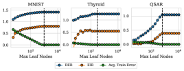
Figure 4: Random forest classifiers. Blacked dashed line represents the interpolation threshold. Across all tasks, $\mathrm{DER}$ and $\mathrm{EIR}$ are maximized at this point, and then remain constant thereafter.

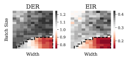
(a) Without LR decay.

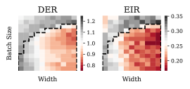
(b) With LR decay.

Figure 5: Large scale studies of deep ensembles on ResNet18/CIFAR-10. We plot the $\mathrm{DER}$, $\mathrm{EIR}$, average error and majority vote error rate across a range of hyper-parameters, for two training settings: one with learning rate decay, and one without. The black dashed line indicates the interpolation threshold, i.e., the curve below which individual models achieve exactly zero training error. Observe that interpolating ensembles attain distinctly lower $\mathrm{EIR}$ than non-interpolating ensembles, and correspondingly have low $\mathrm{DER}$ ($<1$), compared to non-interpolating ensembles with high $\mathrm{DER}$ ($>1$).

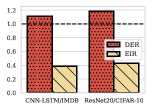
Figure 6: Bayesian ensembles on IMDB and CIFAR-10. These provide examples of ensembles which do not interpolate the training data, and which have high $\mathrm{DER}$ ($>1$) and correspondingly high $\mathrm{EIR}$.

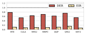
Figure 7: Ensembles of fine-tuned BERT on GLUE tasks. Here the models are large relative to the dataset size, and consequently they exhibit low $\mathrm{DER}$ ($<1$) and $\mathrm{EIR}$ across all tasks.

Interpolating random feature classifiers.

We first look at the bagged random feature ensembles on the MNIST, Thyroid, and QSAR datasets. In Figure 3, we plot the $\mathrm{EIR}$, $\mathrm{DER}$ and training error for each of these ensembles (recall that for ensembles which use bagging, the training error is computed as the in-bag training error). We observe the same phenomenon across these three tasks: as a function of model capacity, the $\mathrm{EIR}$ and $\mathrm{DER}$ are both maximized at the interpolation threshold, before decreasing thereafter. This indicates that much higher-capacity models, those with the ability to easily interpolate the training data, benefit significantly less from ensembling. In particular, observe that for sufficiently high-capacity ensembles, the $\mathrm{DER}$ become less than 1, entering the regime in which our theory guarantees low ensemble improvement.

Interpolating deep ensembles.

We next consider the $\mathrm{DER}$, $\mathrm{EIR}$, average test error, and majority vote test error rates for large-scale empirical evaluations on ResNet18/CIFAR-10 models in batch size/width space, both with and without learning rate decay. See Figure 5 for the results. Note that the use of learning rate decay facilitates easier interpolation of the training data during training, hence broadening the range of hyper-parameters for which interpolation occurs. The figures are colored so that ensembles in the regime $\mathrm{DER}<1$ are in red, while ensembles with $\mathrm{DER}>1$ are in grey. The black dashed line indicates the interpolation threshold, i.e., the curve in hyper-parameter space below which ensembles achieve zero training error (meaning every classifier in the ensemble has zero training error). Observe in particular that, across all settings, all models in the regime $\mathrm{DER}<1$ are interpolating models; and, more generally, that interpolating models tend to exhibit much smaller $\mathrm{DER}$ than non-interpolating models. Observe moreover that there can be a sharp transition between these two regimes, wherein the $\mathrm{DER}$ is large just at the interpolation threshold, and then it quickly decreases beyond that threshold. Correspondingly, ensemble improvement is much less pronounced for interpolating versus more traditional non-interpolating ensembles. This is consistent with results previously observed in the literature, e.g., [GJS⁺20]. We remark also that the behavior observed in Figure 5 exhibits the same phases identified in [YHT⁺21] (an example of phase transitions in learning more generally [EdB01, MM17]), although the $\mathrm{DER}$ itself was not considered in that previous study.

Bayesian neural networks.

Next, we show that Bayesian neural networks benefit significantly from ensembling. In Figure 6, we plot the $\mathrm{DER}$ and $\mathrm{EIR}$ for Bayesian ensembles on the CIFAR-10 and IMDB tasks, using the ResNet20 and CNN-LSTM architectures, respectively. The samples we present here are provided by [INLW21], who use Hamiltonian Monte Carlo to sample accurately from the posterior distribution over models. For both tasks, we observe that both ensembles exhibit $\mathrm{DER}>1$ and high $\mathrm{EIR}$. In light of our findings regarding ensemble improvement and interpolation, we note that the Bayesian ensembles by design do not interpolate the training data (when drawn at non-zero temperature), as the samples are drawn from a distribution not concentrated only on the modes of the training loss. While we do not perform additional experiments with Bayesian neural networks in the present work, evaluating the $\mathrm{DER}$/$\mathrm{EIR}$ as a function of posterior temperature for these models is an interesting direction for future work. We hypothesize that the qualitative effective of decreasing the sampling temperature will be similar to that of increasing the batch size in the plots in Figure 5.

Fine-tuned BERT ensembles.

Here, we present results for ensembles of BERT models fine-tuned on the GLUE classification tasks. These provide examples of a very large model trained on small datasets, on which interpolation is easily possible. For these experiments, we use 25 BERT models pre-trained from independent initializations provided in [SYT⁺22]. Each of these 25 models is then fine-tuned on the 7 classification tasks in the GLUE [WSM⁺19] benchmark set and evaluated on relatively small test sets, ranging in size from  250 (RTE) to  40,000 (QQP) samples. In Figure 7, we plot the $\mathrm{EIR}$ and $\mathrm{DER}$ across these benchmark tasks and observe that, as predicted, the ensemble improvement rate is low and $\mathrm{DER}$ is uniformly low ($<1$).

The unique case of random forests.

Random forests are one of the most widely-used ensembling methods in practice. Here, we show that the effectiveness of ensembling is much greater for random forest models than for highly-parameterized models like the random feature classifiers and the deep ensembles. Note that for random forests, interpolation of the training data is possible, in particular whenever the number of terminal leaf nodes is sufficiently large (where here we again compute the average training error using on the in-bag training examples for each tree), but it is not possible to go “into” the interpolating regime. In Figure 4, we plot the $\mathrm{DER}$, $\mathrm{EIR}$, and training error as a function of the max number of leaf nodes (a measure of model complexity). Before the interpolation threshold, both the $\mathrm{EIR}$ and $\mathrm{DER}$ increase as a function of model capacity, in line with what is observed for the random feature and deep ensembles. However, we observe distinct behavior at the interpolation threshold: both $\mathrm{EIR}$ and $\mathrm{DER}$ become constant past this threshold. This is fundamental to tree-based methods, due to the method by which they are fit, e.g., using a standard procedure like CART [BFSO84]. As soon as a tree achieves zero training error, any impurity method used to split the nodes further is saturated at zero, and therefore the models cannot continue to grow. This indicates that trees are particularly well-suited to ensembling across all hyper-parameter values, in contrast to other parameterized types of classifiers.

6 Discussion and conclusion

To help answer the question of when ensembling is effective, we introduce the ensemble improvement rate ($\mathrm{EIR}$), which we then study both theoretically and empirically. Theoretically, we provide a comprehensive characterization of the $\mathrm{EIR}$ in terms of the disagreement-error ratio $\mathrm{DER}$. The results are based on a new, mild condition called competence, which we introduce to rule out pathological cases that have hampered previous theoretical results. Using a simple first-order analysis, we show that the competence condition is sufficient to guarantee that ensembling cannot hurt performance—something widely observed in practice, but surprisingly unexplained by existing theory. Using a second-order analysis, we are able to theoretically characterize the $\mathrm{EIR}$, by upper and lower bounding it in terms of a linear function of the $\mathrm{DER}$. On the empirical side, we first verify the assumptions of our theory (namely that the competence assumption holds broadly in practice), and we show that our bounds are indeed descriptive of ensemble improvement in practice. We then demonstrate that improvement decreases precipitously for interpolating ensembles, relative to non-interpolating ones, providing a very practical guideline for when to use ensembling.

Our work leaves many directions to explore, of which we name a few promising ones. First, while our theory represents a significant improvement on previous results, there are still directions to extend our analysis. For example, Figure 2 suggests that the relationship between $\mathrm{EIR}$ and $\mathrm{DER}$ can be even more finely characterized. Is it possible to refine our analysis further to incorporate information about the data and/or model architecture? Second, can we formalize the connection between ensemble effectiveness and the interpolation point, and relate it to similar ideas in the literature?

Acknowledgments.

We would like to acknowledge the DOE, IARPA, NSF, and ONR as well as a J. P. Morgan Chase Faculty Research Award for providing partial support of this work.

Appendix A Proofs of our main results

In this section, we provide proofs for our main results. Throughout the section, we denote $\mathbb{P}_{h,h^{\prime}\sim\rho^{2}}$, $\mathbb{P}_{h\sim\rho}$, $\mathbb{E}_{h\sim\rho}$ by $\mathbb{P}_{h,h^{\prime}}$, $\mathbb{P}_{h}$, $\mathbb{E}_{h}$, respectively. We also denote $W_{\rho}(X,Y)$ simply by $W_{\rho}$. We typically omit explicit dependence on the data distribution $\mathcal{D}$ when it is apparent from context.

A.1 Proof of Theorem 1

We first state and prove two lemmas that will be used in the proof of Theorem 1. Our first lemma states that majority-vote error $L_{\mathcal{D}}[h_{\mathrm{MV}}]$ is upper bounded by probability of $W_{\rho}(X,Y)$ being large.

Lemma 1.

There is the inequality $L_{\mathcal{D}}[h_{\mathrm{MV}}]\leq\mathbb{P}_{\mathcal{D}}(W_{\rho}(X,Y)\geq 1/2),$ where $L_{\mathcal{D}}(h)=\mathbb{E}_{\mathcal{D}}[\mathbb{1}(h(X)\neq Y)]$, $h_{\mathrm{MV}}(\bm{x})=\operatorname*{arg\,max}_{j}\;\mathbb{E}_{h}[\mathbb{1}(h(\bm{x})=j)]$ and $W_{\rho}(X,Y)=\mathbb{E}_{h}[\mathbb{1}(h(X)\neq Y)]$.

Proof.

For given data point $x$, $W_{\rho}<1/2$ implies that we are predicting the true label correctly more than half of the time. Thus, the majority vote classifier will correctly predict the label on the data point. ∎

Our next lemma states a property of competent classifiers which plays a crucial role in the main proof.

Lemma 2.

Under Assumption 1 (competence), for any increasing function $h$ satisfying $h(0)=0$,

$$\mathbb{E}_{\mathcal{D}}[h(W_{\rho})\mathbb{1}_{W_{\rho}<1/2}]\;\geq\;\mathbb{E}_{\mathcal{D}}[h(\bar{W_{\rho}})\mathbb{1}_{\bar{W_{\rho}}\leq 1/2}],$$

where $\bar{W_{\rho}}=1-{W_{\rho}}$.

Proof.

For every $x\in[0,1]$,

$$\mathbb{P}_{\mathcal{D}}({W_{\rho}}\mathbb{1}_{{W_{\rho}}<1/2}\geq x) =\mathbb{P}_{\mathcal{D}}({W_{\rho}}\in[x,1/2))\,\mathbb{1}_{x\leq 1/2},$$

$$\mathbb{P}_{\mathcal{D}}(\bar{W_{\rho}}\mathbb{1}_{\bar{W_{\rho}}\leq 1/2}\geq x) =\mathbb{P}_{\mathcal{D}}(\bar{W_{\rho}}\in[x,1/2])\,\mathbb{1}_{x\leq 1/2}=\mathbb{P}_{\mathcal{D}}(W_{\rho}\in[1/2,1-x])\,\mathbb{1}_{x\leq 1/2}.$$

From Assumption 1, this implies that $\mathbb{P}_{\mathcal{D}}({W_{\rho}}\mathbb{1}_{{W_{\rho}}<1/2}\geq x)\geq\mathbb{P}_{\mathcal{D}}(\bar{W_{\rho}}\mathbb{1}_{\bar{W_{\rho}}\leq 1/2}\geq x)$ for all $x\in[0,1]$. Therefore, for any increasing function $h$ satisfying $h(0)=0$, since $h(x\,\mathbb{1}_{x\leq c})=h(x)\mathbb{1}_{x\leq c}$,

$$\mathbb{P}_{\mathcal{D}}(h({W_{\rho}})\mathbb{1}_{{W_{\rho}}<1/2}\geq x)\geq\mathbb{P}_{\mathcal{D}}(h(\bar{W_{\rho}})\mathbb{1}_{\bar{W_{\rho}}\leq 1/2}\geq x).$$

As $W_{\rho}$ is non-negative, the equality $\mathbb{E}X=\int_{0}^{\infty}\mathbb{P}(X\geq x)\mathrm{d}x$ concludes the proof. ∎

With these two lemmas, we now provide the proof of Theorem 1.

Proof of Theorem 1.

From Lemma 1 and the relation $\mathbb{E}_{h}[L_{\mathcal{D}}(h)]=\mathbb{E}_{\mathcal{D}}[W_{\rho}]$ (Fubini’s theorem), it suffices to show that $\mathbb{P}_{\mathcal{D}}(W_{\rho}\geq 1/2)\leq\mathbb{E}_{\mathcal{D}}[W_{\rho}]$. To do so, observe

$$\mathbb{E}_{\mathcal{D}}[(W_{\rho}-1)\mathbb{1}_{W_{\rho}\geq 1/2}]+\mathbb{E}_{\mathcal{D}}[\bar{W_{\rho}}\mathbb{1}_{\bar{W_{\rho}}\leq 1/2}]=\mathbb{E}_{\mathcal{D}}[(W_{\rho}-1)\mathbb{1}_{W_{\rho}\geq 1/2}]+\mathbb{E}_{\mathcal{D}}[(1-W_{\rho})\mathbb{1}_{W_{\rho}\geq 1/2}]=0.$$

Applying Lemma 2 with $h(x)=x$,

$$\mathbb{E}_{\mathcal{D}}[W_{\rho}]-\mathbb{P}_{\mathcal{D}}(W_{\rho}\geq 1/2) \geq\mathbb{E}_{\mathcal{D}}[(W_{\rho}-1)\mathbb{1}_{W_{\rho}\geq 1/2}]+\mathbb{E}_{\mathcal{D}}[W_{\rho}\mathbb{1}_{W_{\rho}<1/2}]$$

$$\geq\mathbb{E}_{\mathcal{D}}[(W_{\rho}-1)\mathbb{1}_{W_{\rho}\geq 1/2}]+\mathbb{E}_{\mathcal{D}}[\bar{W_{\rho}}\mathbb{1}_{\bar{W_{\rho}}\leq 1/2}]=0.$$

which proves

$$L_{\mathcal{D}}[h_{\mathrm{MV}}]\underset{\text{Lemma}\ref{lemma:mv}}{\leq}\mathbb{P}_{\mathcal{D}}(W_{\rho}\geq 1/2){\leq}\mathbb{E}_{\mathcal{D}}[W_{\rho}]=\mathbb{E}_{h}[L_{\mathcal{D}}(h)].$$ (2)

This implies $\mathrm{EIR}\geq 0$. ∎

A.2 Proof of Theorem 2

A.2.1 Lower bound of $\mathrm{EIR}$

To prove the lower bound, we first define the tandem loss, as used in [MLIS20].

Definition 5 (Tandem loss).

Define the tandem loss to be $L(h,h^{\prime})=\mathbb{E}_{\mathcal{D}}[\mathbb{1}(h(X)\neq Y)\mathbb{1}(h^{\prime}(X)\neq Y)]$.

We also rely on the following lemma, which appears as Lemma 2 in [MLIS20]. It provides the connection between the average error rate for each data point, $W_{\rho}$ and the tandem loss, $L(h,h^{\prime})$.

Lemma 3.

The equality $\mathbb{E}_{\mathcal{D}}[{W_{\rho}}^{2}]=\mathbb{E}_{h,h^{\prime}}[L(h,h^{\prime})]$ holds.

We first state and prove the following lemma, which provides an upper bound on the tandem loss.

Lemma 4.

For the $K$-class problem,

$$\mathbb{E}_{h,h^{\prime}}[L(h,h^{\prime})]\leq\frac{2(K-1)}{K}\left(\mathbb{E}_{h}[L(h)]-\frac{1}{2}\mathbb{E}_{h,h^{\prime}}[D(h,h^{\prime})]\right).$$

Proof.

We denote $\mathbb{P}_{h}(h(X)\neq Y)$ by $\bar{h}_{Y}(X)$. Note that $\mathbb{E}_{\mathcal{D}}(1-\bar{h}_{Y}(X))=\mathbb{E}_{h}[L(h)]$ and

$$\mathbb{E}_{h,h^{\prime}}[L(h,h^{\prime})] =\mathbb{E}_{\mathcal{D}}[\mathbb{P}_{h}(h(X)\neq Y)\mathbb{P}_{h^{\prime}}(h^{\prime}(X)\neq Y)]$$

$$=\mathbb{E}_{\mathcal{D}}[(1-\bar{h}_{Y}(X))^{2}].$$

Then we get

$$\mathbb{E}_{h,h^{\prime}}[L(h,h^{\prime})] =\mathbb{E}_{\mathcal{D}}[(1-\bar{h}_{Y}(X))^{2}]$$

$$=1-\mathbb{E}_{\mathcal{D}}[\bar{h}_{Y}(X)]-\mathbb{E}_{\mathcal{D}}[\bar{h}_{Y}(X)(1-\bar{h}_{Y}(X))]$$

$$=\mathbb{E}_{h}[L(h)]-\mathbb{E}_{\mathcal{D}}[\bar{h}_{Y}(X)(1-\bar{h}_{Y}(X))].$$

Now we will derive a lower bound of the second term. Since

$$\mathbb{E}_{h,h^{\prime}}[\mathbb{1}(h(X)\neq h^{\prime}(X))]=\sum_{j}\bar{h}_{j}(X)(1-\bar{h}_{j}(X)),$$

it follows that

$$\bar{h}_{Y}(X)(1-\bar{h}_{Y}(X))=\mathbb{E}_{h,h^{\prime}}[\mathbb{1}(h(X)\neq h^{\prime}(X))]-\sum_{j\neq Y}\bar{h}_{j}(X)(1-\bar{h}_{j}(X)).$$

By maximizing $\sum_{j\neq Y}\bar{h}_{j}(X)(1-\bar{h}_{j}(X))$ subject to $\sum_{j\neq Y}\bar{h}_{j}(X)=1-\bar{h}_{Y}(X)$, we get $\bar{h}_{j}(X)=\frac{1-\bar{h}_{Y}(X)}{K-1}$, which yields the upper bound

$$\sum_{j\neq Y}\bar{h}_{j}(X)(1-\bar{h}_{j}(X))\leq\frac{K-2}{K-1}(1-\bar{h}_{Y}(X))+\frac{1}{K-1}\bar{h}_{Y}(X)(1-\bar{h}_{Y}(X)).$$

It follows that

$$\mathbb{E}_{\mathcal{D}}[\bar{h}_{Y}(X)(1-\bar{h}_{Y}(X))]\geq\frac{K-1}{K}\mathbb{E}_{h,h^{\prime}}[D(h,h^{\prime})]-\frac{K-2}{K}\mathbb{E}_{h}[L(h)],$$

and thus that

$$\mathbb{E}_{h,h^{\prime}}[L(h,h^{\prime})] =\mathbb{E}_{h}[L(h)]-\mathbb{E}_{\mathcal{D}}[\bar{h}_{Y}(X)(1-\bar{h}_{Y}(X))]$$

$$\leq\mathbb{E}_{h}[L(h)]-\left(\frac{K-1}{K}\mathbb{E}_{h,h^{\prime}}[D(h,h^{\prime})]-\frac{K-2}{K}\mathbb{E}_{h}[L(h)]\right)$$

$$=\frac{2(K-1)}{K}\left(\mathbb{E}_{h}[L(h)]-\frac{1}{2}\mathbb{E}_{h,h^{\prime}}[D(h,h^{\prime})]\right).$$

∎

We now provide the proof for the lower bound of $\mathrm{EIR}$ in Theorem 2.

Proof.

We first claim that $\mathbb{P}_{\mathcal{D}}(W_{\rho}\geq 1/2)\leq 2\,\mathbb{E}_{\mathcal{D}}[{W_{\rho}}^{2}]$. Then, we have

$$\mathbb{E}_{\mathcal{D}}[(2{W_{\rho}}^{2}-1)\mathbb{1}_{{W_{\rho}}\geq 1/2}] =\mathbb{E}_{\mathcal{D}}[(2(1-\bar{W_{\rho}})^{2}-1)\mathbb{1}_{\bar{W_{\rho}}\leq 1/2}]$$

$$=\mathbb{E}_{\mathcal{D}}[(1-4\bar{W_{\rho}}+2\bar{W_{\rho}}^{2})\mathbb{1}_{\bar{W_{\rho}}\leq 1/2}],$$

where $\bar{W_{\rho}}=1-{W_{\rho}}$. Therefore,

$$\mathbb{E}_{\mathcal{D}}[(2{W_{\rho}}^{2}-1)\mathbb{1}_{{W_{\rho}}\geq 1/2}]+\mathbb{E}_{\mathcal{D}}[2\bar{W_{\rho}}^{2}\mathbb{1}_{\bar{W_{\rho}}\leq 1/2}] =\mathbb{E}_{\mathcal{D}}[(1-4\bar{W_{\rho}}+4\bar{W_{\rho}}^{2})\mathbb{1}_{\bar{W_{\rho}}\leq 1/2}]\geq 0.$$

Now we apply Lemma 2 with $h(x)=2x^{2}$, to obtain

$$\mathbb{E}_{\mathcal{D}}[2{W_{\rho}}^{2}]-\mathbb{P}_{\mathcal{D}}({W_{\rho}}\geq 1/2) \geq\mathbb{E}_{\mathcal{D}}[(2{W_{\rho}}^{2}-1)\mathbb{1}_{{W_{\rho}}\geq 1/2}]+\mathbb{E}_{\mathcal{D}}[2{W_{\rho}}^{2}\mathbb{1}_{{W_{\rho}}<1/2}]$$ (3)

$$\geq\mathbb{E}_{\mathcal{D}}[(2{W_{\rho}}^{2}-1)\mathbb{1}_{{W_{\rho}}\geq 1/2}]+\mathbb{E}_{\mathcal{D}}[2\bar{W_{\rho}}^{2}\mathbb{1}_{\bar{W_{\rho}}\leq 1/2}]\;\geq 0,$$

which proves the claim, $\mathbb{P}_{\mathcal{D}}(W_{\rho}\geq 1/2)\leq 2\,\mathbb{E}_{\mathcal{D}}[{W_{\rho}}^{2}]$.

Now we put the claim together with Lemmas 1, 3, and 4 to conclude the proof.

$$L(h_{\mathrm{MV}}) \underset{\text{Lemma \ref{lemma:mv}}}{\leq}\mathbb{P}_{\mathcal{D}}(W_{\rho}\geq 1/2)\leq 2\,\mathbb{E}_{\mathcal{D}}[{W_{\rho}}^{2}]\underset{\text{Lemma \ref{lemma:tandem}}}{=}2\,\mathbb{E}_{h,h^{\prime}}[L(h,h^{\prime})]$$ (4)

$$\underset{\text{Lemma \ref{lemma:kclass_tandem_ub}}}{\leq}\frac{4(K-1)}{K}\left(\mathbb{E}_{h}[L(h)]-\frac{1}{2}\mathbb{E}_{h,h^{\prime}}[D(h,h^{\prime})]\right)$$

Rearranging the terms, we obtain

$$\mathbb{E}_{h}[L_{\mathcal{D}}(h)]-L(h_{\mathrm{MV}})\geq\frac{2(K-1)}{K}\mathbb{E}_{h,h^{\prime}}[D(h,h^{\prime})]-\frac{3K-4}{K}\mathbb{E}_{h}[L(h)].$$ (5)

Dividing the both terms by $\mathbb{E}_{h}[L(h)]$ gives the lower bound $\frac{2(K-1)}{K}\mathrm{DER}-\frac{3K-4}{K}$. ∎

A.2.2 Upper bound of $\mathrm{EIR}$

We denote $\mathbb{P}_{h}(h(X)\neq Y)$ by $\bar{h}_{Y}(X)$. We have

$$\mathbb{E}_{h}[L(h)]-L(h_{\mathrm{MV}}) =\mathbb{E}_{h,\mathcal{D}}[\mathbb{1}(h(X)\neq Y)-\mathbb{1}(h_{\mathrm{MV}}(X)\neq Y)].$$

Now

$$\mathbb{1}(h(X)\neq Y)-\mathbb{1}(h_{\mathrm{MV}}(X)\neq Y) =\mathbb{1}(h_{\mathrm{MV}}(X)=Y)-\mathbb{1}(h(X)=Y)$$

$$=\mathbb{1}(h(X)\neq h_{\mathrm{MV}}(X))\left(\mathbb{1}(h_{\mathrm{MV}}(X)=Y)-\mathbb{1}(h(X)=Y)\right)$$

$$\leq\mathbb{1}(h(X)\neq h_{\mathrm{MV}}(X)).$$

Now notice $\mathbb{E}_{h,\mathcal{D}}[\mathbb{1}(h(X)\neq h_{\mathrm{MV}}(X))]=1-\mathbb{E}_{\mathcal{D}}[\max_{k}\bar{h}_{k}(X)]$. Moreover, by Hölder’s inequality,

$$\|\bar{\bm{h}}(X)\|_{2}^{2}\leq\max_{k}\bar{h}_{k}(X),$$

and so

$$\mathbb{E}_{h}[L(h)]-L(h_{\mathrm{MV}}) \leq 1-\mathbb{E}_{\mathcal{D}}[\max_{k}\bar{h}_{k}(X)]$$ (6)

$$\leq 1-\mathbb{E}_{\mathcal{D}}[\|\bar{\bm{h}}(X)\|^{2}]=\mathbb{E}_{h,h^{\prime}}[D(h,h^{\prime})].$$

Dividing the both terms by $\mathbb{E}_{h}[L(h)]$ gives the upper bound $\mathrm{DER}$.

A.3 Upper and lower bounds on the error rate of the majority vote classifier

We now present upper and lower bound on the majority vote classifier that follow from the bounds in Theorem 1 and 2, and compare them with existing bounds in the literature.

Theorem 3.

For any competent ensemble $\rho$ of $K$-class classifiers, the majority vote error rate satisfies

$$L(h_{\mathrm{MV}}) \leq\min\left\{\frac{4(K-1)}{K}\left(\mathbb{E}_{h\sim\rho}[L(h)]-\frac{1}{2}\mathbb{E}_{h,h^{\prime}\sim\rho}[D(h,h^{\prime})]\right)\;,\mathbb{E}_{h\sim\rho}[L(h)]\right\}$$

$$L(h_{\mathrm{MV}}) \geq\mathbb{E}_{h\sim\rho}[L(h)]-\mathbb{E}_{h,h^{\prime}\sim\rho}[D(h,h^{\prime})].$$

Proof.

The upper bound follows from inequality (2) and (4). The lower bound follows from inequality (6). ∎

We have already discussed that the bound $L(h_{\mathrm{MV}})\leq\mathbb{E}[L(h)]$ represents an improvement by a factor of 2 over the naive first-order bound (1). Here, we further compare the bound

$$L(h_{\mathrm{MV}})\leq\frac{4(K-1)}{K}\left(\mathbb{E}_{h\sim\rho}[L(h)]-\frac{1}{2}\mathbb{E}_{h,h^{\prime}\sim\rho}[D(h,h^{\prime})]\right)$$ (7)

to other known results in the literature. The closest in form is a bound specialized to binary case from [MLIS20], which gives

$$L(h_{\mathrm{MV}})\leq 4\mathbb{E}_{h\sim\rho}[L(h)]-2\mathbb{E}_{h,h^{\prime}\sim\rho}[D(h,h^{\prime})].$$ (8)

Note that plugging in $K=2$ to (7), we obtain the bound $2\mathbb{E}_{h\sim\rho}[L(h)]-\mathbb{E}_{h,h^{\prime}\sim\rho}[D(h,h^{\prime})]$, immediately improving on (8) by a factor of 2 (interestingly, the same factor that we save on the first-order bound). Hence, provided the competence assumption holds, our bound is a direct improvement on this bound, and furthermore generalizes directly to the $K$-class setting.

To our knowledge, the sharpest known upper bound on the majority-vote classifier is the general form of the C-bound given in [LMRR17], which states, provided $\mathbb{E}[M_{\rho}(X,Y)]>0$,

$$L(h_{\mathrm{MV}})\leq 1-\frac{\mathbb{E}[M_{\rho}(X,Y)]^{2}}{\mathbb{E}[M_{\rho}^{2}(X,Y)]},$$ (9)

where $M_{\rho}(X,Y)=\mathbb{E}_{h\sim\rho}[\mathbb{1}(h(X)=Y)]-\max_{j\neq Y}\mathbb{E}_{h\sim\rho}[\mathbb{1}(h(X)=j)]$ is called the margin. Unfortunately, the use of the margin function makes direct analytical comparison to our bound difficult. However, the bounds can be compared empirically, where the relevant quantities are estimated on hold-out data. In Figure 8, we compare the value of our bound against the value of the multi-class C-bound, on tasks for which we have verified the competence assumption holds. We find that in all but one case (random forests with MNIST), our bound is superior empirically, sometimes significantly. Interestingly, we observe that our bound does particularly well on tasks with only a few classes. This behavior might be attributed to the constant $\frac{4(K-1)}{K}$ in the upper bound (7) which increases as the number of classes $K$ grows.

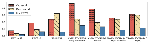
Figure 8: Our bound (7) versus the multi-class C-bound (9).

Appendix B Additional empirical results

B.1 Experimental details

Bagged random feature classifiers.

We consider ensembles of random ReLU feature classifiers, constructed as follows. For each classifier, we draw a random matrix $\bm{U}\in\mathbb{R}^{N\times d}$, whose rows $\bm{u}_{j}$ are drawn from the uniform distribution on the sphere $\mathbb{S}^{d-1}$. For a given input $\bm{x}\in\mathbb{R}^{d}$, we compute the feature $\bm{z}(\bm{x})=\sigma(\bm{Ux})$ where $\sigma(t)=\max(t,0)$ is the ReLU function. We then fit a multi-class logistic regression model in scikit-learn [PVG⁺11] using these (random) features. To form an ensemble of these classifiers, we additionally perform bagging, by sampling a different set of size $n$ with replacement from the training set of size $n$, independently for each individual classifier. Thus, each classifier is subject to two different types of randomness: the randomness from the sampling of the feature matrix $\bm{U}$; and the randomness from the bootstrapping of the training data. For the models shown in the competence plot in Figure 1, we use $500$ random features and $M=100$ classifiers.

Random forests.

We consider random forest (RF) models as implemented in scikit-learn [PVG⁺11], each made up of 20 individual decision trees. We vary the maximum number of leaf nodes in each tree to construct models with varying performance. For the single-ensemble results presented, we use the default parameters implemented in scikit-learn. For the random forests, we use a small version of the MNIST dataset with 5000 randomly selected training examples (500 from each of the 10 classes). We also use two binary classification datasets retrieved from the UCI repository [DG17]: the QSAR oral toxicity dataset (7.2k train, 1.8k test examples, 1024 features) [BGCT19]; and the Thyroid disease dataset (2.5k train, 633 test examples, 21 features) [QCHL87]. For the models shown in the competence plot in Figure 1, we use the default settings of the random forest implementation in scikit-learn.

Deep ensembles.

We consider four different architectures for our deep ensembles. We use a standard ResNet18 models [HZRS16] trained on the CIFAR-10 dataset [KH⁺09], using 100 epochs of SGD with momentum $0.9$, weight decay of $5\times 10^{-4}$ and a learning rate of $0.1$, while varying the batch size and width hyper-parameters. We report results from two variants of this empirical evaluation: one in which we employ learning rate decay (by dropping the learning rate to $0.01$ after 75 epochs); and another in which we disable learning rate decay. For each setting, we train $5$ models from independent initialization to form the respective ensembles. We also evaluate these models on two out-of-distribution databases: CIFAR-10.1 and CIFAR-10-C [RRSS19, HD19] (the latter is itself comprised of 19 different datasets employing various types of data corruption). Finally, we evaluate deep ensembles of 25 standard BERT models [DCLT19], provided with the paper [SYT⁺22], fine-tuned on the GLUE classification tasks [WSM⁺19].

Bayesian ensembles.

For the Bayesian ensembles used in this paper, we consider samples provided in [IVHW21], obtained via large-scale sampling from a Bayesian posterior using Hamiltonian Monte Carlo. To our knowledge, these samples are the most precisely representative of a theoretical Bayesian neural network posterior publicly available. In particular, we use samples on the CIFAR-10 datasets with a ResNet20 architecture, and the IMDB dataset on the CNN-LSTM architecture. We defer to the original paper [IVHW21] for additional details.

B.2 More competence plots

In this section, we provide additional empirical results. To further verify that the competence assumption holds broadly in practice, here we include several more examples of competence plots for experiments presented in the main text.

ResNet18 on CIFAR-10 OOD variants.

In Figures 9 and 10, we plot competence plots for the ResNet18 ensembles on the CIFAR-10, CIFAR-10.1 and a subset of the CIFAR-10-C datasets [RRSS19, HD19]. We find that the competence assumption holds across all examples.

Fine-tuned BERT models.

In Figure 11, we provide competence plots for the BERT/GLUE fine-tuning tasks. For the RTE, CoLA, MNLI, QQP and QNLI tasks, we find that the competence assumption holds. However, we find two examples here where it does not: the MRPC and SST-2 tasks, although the extent to which the assumption is violated in minor. Since these are particularly small datasets, this may also be a product of noise from low sample size.

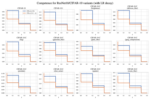
Figure 9: Competence for ResNet18/CIFAR-10 variants (models with learning rate decay). We observe that the competence assumption holds across all tasks.

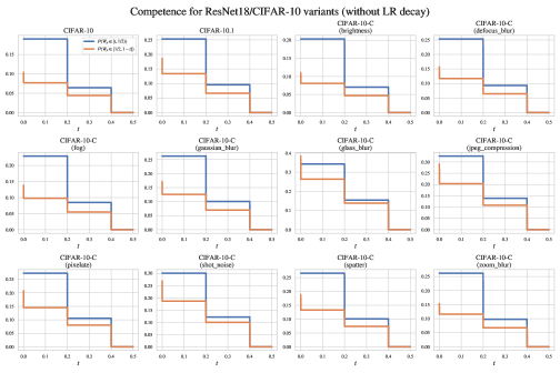
Figure 10: Competence for ResNet18/CIFAR-10 variants (models without learning rate decay). We observe that the competence assumption holds across all tasks.

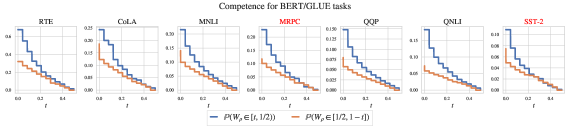
Figure 11: Competence for BERT/GLUE fine-tuning tasks. The competence assumption holds for the RTE, CoLA, MNLI, QQP and QNLI tasks, though interestingly, we find that the competence assumption is (to a small degree) violated for two of the tasks: MRPC and SST-2.

Appendix C Pathological ensembles satisfying $L(h_{\mathrm{MV}})=2\mathbb{E}[L(h)]$

In this section, we provide two pathological examples of ensembles that makes the “first-order” upper bound tight. In particular, the second example shows that positive margin condition, i.e., $\mathbb{E}[M_{\rho}(X,Y)]>0$ where $M_{\rho}(X,Y)=\mathbb{E}_{h\sim\rho}[\mathbb{1}(h(X)=Y)]-\max_{j\neq Y}\mathbb{E}_{h\sim\rho}[\mathbb{1}(h(X)=j)]$, from existing literature is not enough to rule out pathological cases. Recall that the first-order bound introduced in Section 2.2 is the following:

$$0\leq L(h_{\mathrm{MV}})\leq\mathbb{P}(W_{\rho}\geq 1/2)\leq 2\,\mathbb{E}[W_{\rho}]=2\,\mathbb{E}_{h\sim\rho}[L(h)].$$

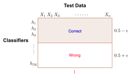
(a) Composition of classifiers in Example 1

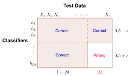
(b) Composition of classifiers in Example 2

Figure 12: Illustration of the composition of classifiers given in Examples 1 and 2. On each plot, the area of the white box equals to the average test error rate. On Figure 12(a), the majority vote error rate is $1$, while the average test error rate is $0.5+\epsilon$. On Figure 12(b), the majority vote error rate is $2\delta$ (Rightmost $2\delta$ test data) while the average test error rate is $\delta(1+2\epsilon)$. The margin of each composition of classifiers is $2\epsilon\to 0$ and $1-2\delta(1+2\epsilon)>0$, respectively.

Example 1 (The first-order upper bound is tight).

Consider a classification problem with two classes. For given $\epsilon>0$, suppose slightly less than half, $0.5-\epsilon$, fraction of classifiers are the perfect classifier, correctly classifying test data with probability 1, and the other $0.5+\epsilon$ fraction of classifiers are completely wrong, incorrectly predicting on test data with probability 1. With this composition of classifiers, the average error rate is $0.5+\epsilon$ and the majority vote error rate is $1$. Taking $\epsilon\to 0$ concludes that the first-order upper bound (1) is tight. A visual illustration of the composition of classifiers is given in Figure 12(a).

The condition $\mathbb{E}[M_{\rho}(X,Y)]>0$ rules out the ensemble described in Example 1. Nonetheless, the first-order bound $2\mathbb{E}[L(h)]$ is tight even when $\mathbb{E}[M_{\rho}(X,Y)]>0$ is satisfied, as we show with the following example.

Example 2 (The first-order upper bound is tight even when the margin is large).

We again consider a classification problem with two classes. For given $\epsilon>0$, as in Example 1, slightly less than half, $0.5-\epsilon$, fraction of classifiers are the perfect classifier. All of the other $0.5+\epsilon$ fraction of classifiers, on the contrary, now correctly predict on the same $1-2\delta$ fraction of the test data and incorrectly predict on the other $2\delta$ fraction of the test data. With this composition of classifiers, the majority vote error rate is $2\delta$ even when the average error rate is $\delta(1+2\epsilon)$. In addition, unlike the composition of classifiers in Example 1, the margin of which is $2\epsilon$, the margin of the new composition of classifiers is $1-2\delta(1+2\epsilon)$, which can be any value smaller than $1$. Taking $\epsilon\to 0$ concludes that the first-order upper bound (1) is also tight when the margin is arbitrarily high. A visual illustration of the composition of classifiers is given in Figure 12(b).

References

- [ABP+22] Taiga Abe, E. Kelly Buchanan, Geoff Pleiss, Richard Zemel, and John Patrick Cunningham. Deep ensembles work, but are they necessary? In Advances in Neural Information Processing Systems, 2022.
- [ABPC22] Taiga Abe, E Kelly Buchanan, Geoff Pleiss, and John Patrick Cunningham. The best deep ensembles sacrifice predictive diversity. In I Can’t Believe It’s Not Better Workshop: Understanding Deep Learning Through Empirical Falsification, 2022.
- [ALMV20] Arsenii Ashukha, Alexander Lyzhov, Dmitry Molchanov, and Dmitry Vetrov. Pitfalls of in-domain uncertainty estimation and ensembling in deep learning. International Conference on Learning Representations (ICLR), 2020.
- [BCNM06] Cristian Buciluǎ, Rich Caruana, and Alexandru Niculescu-Mizil. Model compression. In Proceedings of the 12th ACM SIGKDD international conference on Knowledge discovery and data mining, pages 535–541, 2006.
- [BFSO84] Leo Breiman, Jerome Friedman, Charles J. Stone, and R.A. Olshen. Classification and Regression Trees. Chapman and Hall/CRC, 1984.
- [BGCT19] Davide Ballabio, Francesca Grisoni, Viviana Consonni, and Roberto Todeschini. Integrated qsar models to predict acute oral systemic toxicity. Molecular Informatics, 38(8-9):1800124, 2019.
- [BHMM19] M. Belkin, D. Hsu, S. Ma, and S. Mandal. Reconciling modern machine-learning practice and the classical bias–variance trade-off. Proc. Natl. Acad. Sci. USA, 116:15849–15854, 2019.
- [Bre01] Leo Breiman. Random forests. Machine learning, 45(1):5–32, 2001.
- [CG16] Tianqi Chen and Carlos Guestrin. Xgboost: A scalable tree boosting system. In Proceedings of the 22nd acm sigkdd international conference on knowledge discovery and data mining, pages 785–794, 2016.
- [Con85] Marquis de Condorcet. Essay on the application of analysis to the probability of majority decisions. Paris: Imprimerie Royale, 1785.
- [DCLT19] Jacob Devlin, Ming-Wei Chang, Kenton Lee, and Kristina Toutanova. BERT: Pre-training of deep bidirectional transformers for language understanding. In Proceedings of the 2019 Conference of the North American Chapter of the Association for Computational Linguistics: Human Language Technologies, pages 4171–4186, June 2019.
- [Den12] Li Deng. The mnist database of handwritten digit images for machine learning research. IEEE Signal Processing Magazine, 29(6):141–142, 2012.
- [DG17] Dheeru Dua and Casey Graff. UCI machine learning repository, 2017.
- [EdB01] A. Engel and C. P. L. Van den Broeck. Statistical mechanics of learning. Cambridge University Press, 2001.
- [FHL19] Stanislav Fort, Huiyi Hu, and Balaji Lakshminarayanan. Deep ensembles: A loss landscape perspective. arXiv preprint arXiv:1912.02757, 2019.
- [GJS+20] Mario Geiger, Arthur Jacot, Stefano Spigler, Franck Gabriel, Levent Sagun, Stéphane d’Ascoli, Giulio Biroli, Clément Hongler, and Matthieu Wyart. Scaling description of generalization with number of parameters in deep learning. Journal of Statistical Mechanics: Theory and Experiment, 2020(2):023401, 2020.
- [GLL+15] Pascal Germain, Alexandre Lacasse, Francois Laviolette, Mario March, and Jean-Francis Roy. Risk bounds for the majority vote: From a PAC-Bayesian analysis to a learning algorithm. Journal of Machine Learning Research, 16(26):787–860, 2015.
- [HD19] Dan Hendrycks and Thomas Dietterich. Benchmarking neural network robustness to common corruptions and perturbations. Proceedings of the International Conference on Learning Representations, 2019.
- [HVD+15] Geoffrey Hinton, Oriol Vinyals, Jeff Dean, et al. Distilling the knowledge in a neural network. arXiv preprint arXiv:1503.02531, 2(7), 2015.
- [HZRS16] Kaiming He, Xiangyu Zhang, Shaoqing Ren, and Jian Sun. Deep residual learning for image recognition. In Proceedings of the IEEE conference on computer vision and pattern recognition, pages 770–778, 2016.
- [INLW21] Pavel Izmailov, Patrick Nicholson, Sanae Lotfi, and Andrew G Wilson. Dangers of Bayesian model averaging under covariate shift. Advances in Neural Information Processing Systems, 34:3309–3322, 2021.
- [IVHW21] Pavel Izmailov, Sharad Vikram, Matthew D Hoffman, and Andrew Gordon Gordon Wilson. What are Bayesian neural network posteriors really like? In Proceedings of the 38th International Conference on Machine Learning, volume 139 of Proceedings of Machine Learning Research, pages 4629–4640. PMLR, 18–24 Jul 2021.
- [KH+09] Alex Krizhevsky, Geoffrey Hinton, et al. Learning multiple layers of features from tiny images. 2009.
- [LMRR17] François Laviolette, Emilie Morvant, Liva Ralaivola, and Jean-Francis Roy. Risk upper bounds for general ensemble methods with an application to multiclass classification. Neurocomputing, 219:15–25, 2017.
- [LPB17] Balaji Lakshminarayanan, Alexander Pritzel, and Charles Blundell. Simple and scalable predictive uncertainty estimation using deep ensembles. Advances in neural information processing systems, 30, 2017.
- [MDP+11] Andrew L. Maas, Raymond E. Daly, Peter T. Pham, Dan Huang, Andrew Y. Ng, and Christopher Potts. Learning word vectors for sentiment analysis. In Proceedings of the 49th Annual Meeting of the Association for Computational Linguistics: Human Language Technologies, pages 142–150, June 2011.
- [MLIS20] Andres Masegosa, Stephan Lorenzen, Christian Igel, and Yevgeny Seldin. Second order PAC-Bayesian bounds for the weighted majority vote. In Advances in Neural Information Processing Systems, volume 33, pages 5263–5273, 2020.
- [MM17] C. H. Martin and M. W. Mahoney. Rethinking generalization requires revisiting old ideas: statistical mechanics approaches and complex learning behavior. Technical Report Preprint: arXiv:1710.09553, 2017.
- [OCnM22] Luis A. Ortega, Rafael Cabañas, and Andres Masegosa. Diversity and generalization in neural network ensembles. In Proceedings of The 25th International Conference on Artificial Intelligence and Statistics, volume 151 of Proceedings of Machine Learning Research, pages 11720–11743, 28–30 Mar 2022.
- [OFR+19] Yaniv Ovadia, Emily Fertig, Jie Ren, Zachary Nado, David Sculley, Sebastian Nowozin, Joshua Dillon, Balaji Lakshminarayanan, and Jasper Snoek. Can you trust your model’s uncertainty? evaluating predictive uncertainty under dataset shift. Advances in neural information processing systems, 32, 2019.
- [PVG+11] F. Pedregosa, G. Varoquaux, A. Gramfort, V. Michel, B. Thirion, O. Grisel, M. Blondel, P. Prettenhofer, R. Weiss, V. Dubourg, J. Vanderplas, A. Passos, D. Cournapeau, M. Brucher, M. Perrot, and E. Duchesnay. Scikit-learn: Machine learning in Python. Journal of Machine Learning Research, 12:2825–2830, 2011.
- [QCHL87] J. R. Quinlan, P. J. Compton, K. A. Horn, and L. Lazarus. Inductive knowledge acquisition: A case study. In Proceedings of the Second Australian Conference on Applications of Expert Systems, page 137–156, USA, 1987. Addison-Wesley Longman Publishing Co., Inc.
- [RRSS19] Benjamin Recht, Rebecca Roelofs, Ludwig Schmidt, and Vaishaal Shankar. Do ImageNet classifiers generalize to ImageNet? In Kamalika Chaudhuri and Ruslan Salakhutdinov, editors, Proceedings of the 36th International Conference on Machine Learning, volume 97 of Proceedings of Machine Learning Research, pages 5389–5400. PMLR, 09–15 Jun 2019.
- [SYT+22] Thibault Sellam, Steve Yadlowsky, Ian Tenney, Jason Wei, Naomi Saphra, Alexander D’Amour, Tal Linzen, Jasmijn Bastings, Iulia Raluca Turc, Jacob Eisenstein, Dipanjan Das, and Ellie Pavlick. The multiBERTs: BERT reproductions for robustness analysis. In International Conference on Learning Representations, 2022.
- [TKM21] Ryan Theisen, Jason Klusowski, and Michael Mahoney. Good classifiers are abundant in the interpolating regime. In Arindam Banerjee and Kenji Fukumizu, editors, Proceedings of The 24th International Conference on Artificial Intelligence and Statistics, volume 130 of Proceedings of Machine Learning Research, pages 3376–3384. PMLR, 13–15 Apr 2021.
- [WSM+19] Alex Wang, Amanpreet Singh, Julian Michael, Felix Hill, Omer Levy, and Samuel R. Bowman. GLUE: A multi-task benchmark and analysis platform for natural language understanding. In International Conference on Learning Representations, 2019.
- [YHT+21] Yaoqing Yang, Liam Hodgkinson, Ryan Theisen, Joe Zou, Joseph E Gonzalez, Kannan Ramchandran, and Michael W Mahoney. Taxonomizing local versus global structure in neural network loss landscapes. In Advances in Neural Information Processing Systems, volume 34, pages 18722–18733, 2021.