Uniform Pricing vs Pay as Bid in 100%-Renewables Electricity Markets: A Game-theoretical Analysis

Abstract.

This paper evaluates market equilibrium under different pricing mechanisms in a two-settlement 100%-renewables electricity market. Given general probability distributions of renewable energy, we establish game-theoretical models to analyze equilibrium bidding strategies, market prices, and profits under uniform pricing (UP) and pay-as-bid pricing (PAB). We prove that UP can incentivize suppliers to withhold bidding quantities and lead to price spikes. PAB can reduce the market price, but it may lead to a mixed-strategy price equilibrium. Then, we present a regulated uniform pricing scheme (RUP) based on suppliers’ marginal costs that include penalty costs for real-time deviations. We show that RUP can achieve lower yet positive prices and profits compared with PAB in a duopoly market, which approximates the least-cost system outcome. Simulations with synthetic and real data find that under PAB and RUP, higher uncertainty of renewables and real-time shortage penalty prices can increase the market price by encouraging lower bidding quantities, thereby increasing suppliers’ profits.

1. Introduction

Uniform pricing (UP) is a widely adopted auction design in deregulated electricity markets. The clearing market price under UP is identical to all the suppliers (in one location or zone), regardless of their bidding offers (Kirschen and Strbac, 2018). If there exists no market power, UP can achieve market efficiency (Schweppe et al., 2013), and is also transparent in terms of selecting the least-cost suppliers (Lin and Magnago, 2017). In practice, suppliers can exercise market power, such as reporting a price higher than its marginal cost or withholding capacity, to increase the market price (Kahn et al., 2001)(Zhao et al., 2022). For conventional dispatchable generators, it may not be difficult for the market monitor to mitigate market power by comparing offers to marginal costs and generation capacities (Graf et al., 2021).

However, the UP mechanism still faces some challenges when variable renewable energy (VRE) dominates the market. First, VRE has zero marginal costs, which may cause low and volatile day-ahead market prices if suppliers bid at true marginal costs (Leslie et al., 2020). Second, VRE generation is variable and uncertain. Re-balancing due to uncertain outputs may cause substantial real-time costs. The above two considerations may aggravate profit losses to suppliers and encourage strategic behaviors, e.g., withholding bidding quantities, to increase market prices. There are discussions around allowing VRE suppliers to offer at prices higher than zero marginal costs (Shen and Ilic, 2023). However, since the re-balancing cost and generation capacity of VRE are uncertain and variable, it is challenging for the market monitor to assess what constitutes competitive bidding.

The challenges of implementing UP under high VRE levels open doors for discussing other auction designs, such as pay-as-bid pricing (PAB), where suppliers are paid directly at bidding prices. By introducing price competition, PAB may reduce the average market prices and revenues compared with UP and thus benefit consumers (Son et al., 2004)(Fabra et al., 2006)(Bashi et al., 2018). One drawback of PAB is that it may fail to reveal the true marginal costs of suppliers and thus leads to market inefficiency (Akbari-Dibavar et al., 2020). The market price under PAB is also hard to predict and regulate (Heim and Götz, 2021). However, since VRE suppliers’ re-balancing cost and generation capacity are uncertain, UP may also face similar challenges to PAB under high penetration levels of VRE.

Electricity market design for high penetration levels of VRE is still an open question, and the literature on equilibrium analysis under PAB and UP is under-explored. Son et al. (Son et al., 2004) analyzed the Nash equilibrium of suppliers’ bidding strategies based on game theory but did not take into account uncertainty from VRE. In contrast, some works analyzed the Nash equilibrium of VRE suppliers’ bidding strategies. Ju et al. (Ju et al., 2022) and Taylor et al. (Taylor and Mathieu, 2016) focused on UP and PAB, respectively, which both only focused on the single-settlement market and neglected uncertainty-related costs in real time. Zhao et al. (Zhao et al., 2019) analyzed the market equilibrium under PAB for VRE considering real-time penalty costs. However, the work did not characterize the equilibrium under UP nor make a comparison between UP and PAB. In contrast, in this paper, we provide an analysis of market equilibrium under UP and compare it with PAB. We also propose a regulated uniform pricing scheme (RUP) that takes into account real-time deviation costs. We summarize the contributions of this paper in the following.

Nash equilibrium analysis in a two-settlement market with VRE only: We evaluate the strategic behaviors of suppliers in VRE-only markets, which takes account of day-ahead revenues and real-time shortage penalty costs. We establish game-theoretical frameworks to model suppliers’ bidding strategies under UP and PAB. Given general probability distributions of VRE, we characterize the Nash equilibrium of suppliers’ bidding prices and quantities, and analyze equilibrium market prices and profits.

Market mechanism comparison: We compare equilibrium prices and profits under UP and PAB. We prove that under UP suppliers can exercise market power to cause price spikes. PAB can reduce the market price compared with UP by differentiating prices. However, no pure strategy equilibrium exists under PAB. We propose RUP as a potential regulation benchmark for renewable energy, which can achieve lower yet positive prices and profits compared with PAB under duopoly competition.

Simulation insights: We utilize both synthetic- and real-world data to perform simulations, which show that RUP leads to the lowest market prices and profits. We also observe that under PAB and RUP, higher uncertainty in VRE and a higher real-time penalty price may increase market prices by encouraging conservative bidding quantities thereby increasing suppliers’ profits.

2. System model

We introduce the model of renewable-energy suppliers, the setting of electricity markets, and some assumptions.

We consider a 100%-VRE electricity market (e.g., solar and wind), where a set of VRE suppliers is denoted by $\mathcal{I}=\{1,2,...,I\}$. In the rest of the paper, we use suppliers to refer to VRE suppliers. For one certain hour, the output of supplier $i\in\mathcal{I}$ is denoted as a random variable $X_{i}$, which has the support over $[0,\overline{X}_{i}]$. We assume that the random generation $X_{i}$ has a continuous cumulative distribution function (CDF) $F_{i}$ with the probability density function (PDF) $f_{i}$. We assume zero marginal production costs for VRE suppliers.

We model a two-settlement electricity market, which consists of a day-ahead market (DAM) and a real-time market (RTM) (Bitar et al., 2012). In the DAM, any supplier $i$ submits the bidding price $p_{i}$ with a cap $\bar{p}$, quantity $q_{i}$, or supply curve $Q_{i}(\cdot)$ to the system operator. Based on suppliers’ bidding strategies and demand $D$, the system operator clears the market with the price $\pi_{i}$ and supplier delivery commitment $\bm{x}=(x_{i},i\in\mathcal{I})$. In the RTM, if supplier $i$’s actual generation falls short of the committed quantity, i.e., $x_{i}>X_{i}$, it needs to pay the real-time penalty price $\lambda$, resulting in the penalty cost $\lambda(x_{i}-X_{i})$. We assume that $\lambda>0$ is fixed (or the expected value of the random penalty price independent of random generations). Such a penalty cost will reflect the cost of other flexible resources addressing the deviation. Overall, the profit of supplier $i$ is

(1) $$R_{i}= x_{i}\cdot\pi_{i}-\mathbb{E}_{X_{i}}\left[\lambda\cdot(x_{i}-X_{i})^{+}\right].$$

We clarify some assumptions in this paper which we will further generalize in future work.

Assumption 1.

(i) The system demand $D>0$ is fixed and inelastic; (ii) The penalty price is positive, i.e., $\lambda>0$; (iii) There is no reward or penalty on the excessive generation (i.e., $x_{i}<X_{i}$) in real time, and the excessive generations are simply curtailed; (iv) Suppliers are price-takers in the RTM; (v) Suppliers have complete market information.

In Sections 3- 5, we will discuss different market clearing mechanisms in the day-ahead market: UP, PAB, and RUP, respectively. We will analyze the equilibrium market price and profits based on game-theoretical models.

3. Uniform pricing

We will characterize the Nash equilibrium of suppliers’ bidding prices and quantities under UP.

Before going into details, we will first present an optimal day-ahead commitment for suppliers based on the cleared price, which can help analyze bidding quantities under different mechanisms later. Based on the profit formulation (1), Lemma 1 characterizes the optimal day-ahead committed quantity.

Lemma 1 (optimal commitment).

If supplier $i$ is paid at the price $\pi_{i}$ in the DAM, the cleared commitment $x_{i}=y_{i}^{*}(\pi_{i})$ in the following will maximize its profit.

(2) $$y_{i}^{*}(\pi_{i})=F_{i}^{-1}\left(\min(\frac{\pi_{i}}{\lambda},1)\right).$$

Lemma 1 is easily proved based on the first order condition of (1). Here $y_{i}^{*}(\pi_{i})$ is non-decreasing over $\pi_{i}\in[0,\bar{p}]$. When the price is zero, any supplier should commit zero quantity in the DAM and zero profits, i.e., $y_{i}^{*}(0)=0$ to avoid penalty costs in real time. If $\pi_{i}\geq\lambda$, the supplier will just bid the maximum quantity $\overline{X}_{i}$. Next, under UP, we will first consider that suppliers are required to bid zero prices and then generalize it to any prices in Appendix B.

3.1. Pricing mechanism

Each supplier bids the price $p_{i}=0$ and quantity $q_{i}\geq 0$. The clearing price $\pi^{*}$ and commitment $\bm{x}^{*}$ are characterized in the following.

(3a) $$\text{If~{}}\sum_{i}q_{i}\leq D,\pi^{*}=\bar{p}\text{~{}and~{}}x_{i}^{*}=q_{i}.$$

(3b) $$\text{If~{}}\sum_{i}q_{i}>D,\pi^{*}=0\text{~{}and~{}}\sum_{i\in\mathcal{I}}x_{i}^{*}=D.$$

This mechanism leads to bipolar prices. Note that at the point $\sum_{i}q_{i}=D$, the market price is not continuous. To maintain a pure strategy Nash equilibrium, we consider that the market price is right-continuous in $\sum_{i}q_{i}$, i.e., $\pi=\bar{p}$ when $\sum_{i}q_{i}=D$.

3.2. Game-theoretical model

Each supplier $i$ decides on the bidding quantity $q_{i}\geq 0$ to maximize its profit. We formulate a game-theoretical model as suppliers’ decisions are coupled due to the market clearing price.

• Players: Suppliers $\mathcal{I}$

• Strategy: Bidding quantity $0\leq q_{i}\leq\overline{X}_{i}$ of supplier $i$

• Payoff: Profit $R_{i}$ of supplier $i$

  (4) $$R_{i}(q_{i},q_{-i})=x_{i}^{*}(\bm{q})\cdot\pi^{*}(\bm{q})-\mathbb{E}_{X_{i}}\left[\lambda\cdot(x_{i}^{*}(\bm{q})-X_{i})^{+}\right],$$

  where $\pi^{*}$ and $\bm{x}^{*}$ are given by (3).

Definition 1 defines the pure-strategy bidding-quantity equilibrium of suppliers, where no supplier can increase its profit through unilateral deviation.

Definition 1 (pure quantity equilibrium).

A bidding quantity vector $\bm{q}^{*}$ is a pure price equilibrium if for any supplier $i\in\mathcal{I}$,

(5) $$R_{i}\left({q}_{i}^{*},{q}_{-i}^{*}\right)\geq R_{i}\left({q}_{i},{q}_{-i}^{*}\right),~{}\forall q_{i}\geq 0.$$

3.3. Nash equilibrium

The Nash equilibrium of bidding quantities is affected by supply and demand. First, if there is supply shortage, i.e., $\sum_{i}y_{i}^{*}({\bar{p}})\leq D$, any supplier $i$ just bids the quantity at $y_{i}^{*}({\bar{p}})$, which leads to the price cap $\bar{p}$. It means there is not enough generation capacity in the market. However, if there is adequate supply, i.e., $\sum_{i}y_{i}^{*}({\bar{p}})>D$, the Nash equilibrium is given as follows.

Proposition 1 (Equilibrium bidding quantity $\bm{q}^{*}$).

If $\sum_{i}y_{i}^{*}(\bar{p})>D$, the following conditions give a Nash equilibrium.

(6) $$\text{(i)}~{}\sum_{i}q_{i}^{*}=D;~{}\text{(ii)}~{}0\leq q_{i}^{*}\leq y_{i}^{*}(\bar{p}),\forall i\in\mathcal{I},$$

where the market clearing price is $\pi^{*}=\bar{p}$. Furthermore, all the Nash equilibria satisfy $\pi^{*}=\bar{p}$ and $\sum_{i}q_{i}^{*}=D$.

We show the proof in Appendix A. Proposition 1 shows that the total bidding quantity of suppliers is exactly at the demand $D$, which achieves the price cap $\bar{p}$. Excessive bidding leads to zero price and deficit bidding will encourage some suppliers to bid more. Since suppliers bid the same zero price, it is not unique how to determine the merit order. Theoretically, some suppliers can get a larger share of demand while some get a much smaller one.

Although most current markets require suppliers to bid at marginal costs, they cannot fully capture the cost incurred by renewables’ uncertainty in real time. Therefore, we further generalize the setting in Appendix B and allow suppliers to bid any price instead of zero. One Nash equilibrium in the generalized case will coincide with Proposition 1 at bidding price zero $p_{i}^{*}=0,\forall i$, where the clearing price reaches the price cap $\bar{p}$.

In summary, under UP, suppliers can easily exercise market power to incur high prices. Since suppliers have zero marginal costs with uncertain generations, it can be harder for the market monitor to regulate compared to conventional generators.

4. Pay-as-bid pricing

Next, we will introduce the PAB mechanism, corresponding game-theoretical model, and analysis of Nash equilibrium.

Under PAB, suppliers are paid at their bidding prices. Each supplier $i$ decides the bidding price $0\leq p_{i}\leq\bar{p}$ and bidding quantity $0\leq q_{i}$ to maximize its profit $R_{i}$.

(7) $$R_{i}\left(\bm{p},\bm{q}\right)= x^{*}(\bm{p},\bm{q})\cdot p_{i}-\mathbb{E}_{X_{i}}\left[\lambda\cdot(x^{*}(\bm{p},\bm{q})-X_{i})^{+}\right],$$

where the commitment $\bm{x}^{*}$ follows the merit order given by the solution to Problem MO in Appendix B.

For the Nash equilibrium, first, if there is supply shortage $\sum_{i}y_{i}^{*}({\bar{p}})\leq D$, any supplier $i$ just bids the quantity at $y_{i}^{*}({\bar{p}})$ and the price cap $\bar{p}$. Then, if $\sum_{i}y_{i}^{*}({\bar{p}})>D$, the Nash equilibrium results have been discussed in (Zhao et al., 2019). In summary, for the bidding quantity, there is a weakly dominant strategy $q_{i}^{*}=\bm{y}^{*}({p}_{i})$ for supplier $i$ given its bidding price. For the price equilibrium, however, there is no pure-strategy price equilibrium, but a mixed price equilibrium exists.

The equilibrium price under PAB is lower than the price cap $\bar{p}$. However, it is challenging to characterize or predict in practice the mixed price equilibrium under general probability distributions of renewables. Also, a finite number of suppliers may still have market power to set a high price. Next, we examine a regulated supply-curve-based uniform pricing (RUP), which can further reduce the market price and provide benefits to consumers.

5. Supply-curve-based uniform pricing

Under RUP, any supplier $i$ truthfully reports its inverse CDF function $F_{i}^{-1}(\cdot)$ of random generations, based on which we have $y_{i}^{*}(\cdot)$ as the supply curve. The system operator sets up the cumulative supply curve $Q(p)$.

(8) $$Q(p)=\sum_{i\in\mathcal{I}}y_{i}^{*}({p}),~{}p\leq\bar{p}.$$

The operator clears the market with price $\pi^{*}$: If $Q(\bar{p})\geq D$, then $\pi^{*}$ is achieved at $Q(\pi^{*})=D$. If $Q(\bar{p})<D$, then $\pi^{*}$ is achieved at $\bar{p}$ and the capacity is not adequate.

We build the connection between RUP and a benchmark of near-least system cost in Proposition 2.

Proposition 2.

The cleared day-ahead commitment and market price under RUP give the optimal primal solution $\bm{x}^{*}$ and dual solution $\pi^{e}$, respectively, to the following problem.

(9a) $$\min_{\bm{x}} \sum_{i\in\mathcal{I}}\mathbb{E}_{X_{i}}\left[\lambda\cdot(x_{i}-X_{i})^{+}\right]+\bar{p}\cdot x_{0}$$

(9b) $$\sum_{i\in\mathcal{I}}x_{i}+x_{0}=D,\hskip 107.63855pt:\pi^{e}$$

(9c) $$x_{0}\geq 0,x_{i}\geq 0,\forall i\in\mathcal{I},$$

where $x_{0}$ denotes the lost load.

The above proposition is easily proven based on KKT conditions. If suppliers’ generation variables are independent, the objective function (9a) is exactly the system cost. Since suppliers make decisions based on their own generations, the generation correlation between suppliers cannot be captured. Future work will consider how to distribute the correlation information among suppliers.

This mechanism captures the total marginal cost across the DAM and RTM, making it suitable as a regulation benchmark. First, it approximates the least-cost system solution. Second, each supplier’s profit is maximized at the clearing price. Third, the clearing price is easily obtained compared with the mixed price equilibrium in PAB. Lastly, it will lead to lower prices compared with UP and PAB. If we consider a duopoly case, the price under RUP (denoted by $\pi^{\text{RUP}}$) is lower than the minimum expected equilibrium price of two suppliers ($\pi^{\text{PAB}}$) under PAB. We compare the prices in the following proposition, which is proved in Appendix C.

Proposition 3 (Equilibrium price comparison).

Considering a duopoly market, the equilibrium (expected) market price satisfies

(10) $$\bar{p}\geq\pi^{\text{PAB}}\geq\pi^{\text{RUP}}>0.$$

If suppliers can report any supply curve, the Nash equilibrium in Proposition 4 under uniform pricing is one possible result. The system operator needs to monitor and evaluate the generation information of generators to mitigate market power.

6. Simulation results

We simulate the results of market prices and suppliers’ profits under UP, PAB, and RUP of two suppliers. The results show that RUP leads to the lowest price and profits for suppliers. We investigate the impact of generation uncertainty and real-time penalty price based on synthetic data and real data, respectively.

We simulate two case studies: (i) we assume a truncated normal distribution of suppliers’ renewable-energy generations and examine how the market price and suppliers’ profits will change with generation uncertainty ; (ii) we use historical real data to establish the probability distribution of generations and investigate the impact of real-time penalty prices. We set demand at 2MW and set the bidding price cap at $\bar{p}=1$k$/MWh.

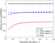
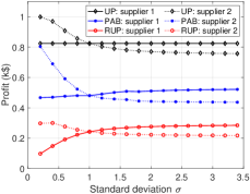
Figure 1. (a) Equilibrium price; (b) Equilibrium profit. Both are with supplier 2’s standard deviation of generations.

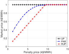
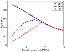
Figure 2. (a) Equilibrium price; (b) Equilibrium profit, as a function of penalty price.

6.1. Synthetic data

6.1.1. Setup

For both suppliers, we assume their generations follow normal distributions with a mean value of 1.5MW, which are truncated between [0,3] MW. We fix supplier 1’s standard deviation (std) at 1MW and vary supplier 2’s. We set the real-time penalty price at $\lambda=1.5$k$/MWh and assume two suppliers equally share the demand under UP.

6.1.2. Results

We show that UP can lead to the highest prices and profits for suppliers. Also, Under both PAB and RUP, one supplier’s increased generation uncertainty will reduce its own profit and increase the other supplier’s profit.

In Figures 1, we show equilibrium market prices in (a) and profits in (b) by varying supplier 2’s std of generations. UP will always lead to price cap $\bar{p}$ (black curve) in Figure 1(a) and highest profits (black curve) in Figure 1(b). As we assume that two suppliers equally share the demand, supplier 1’s profit (black solid curve) remains constant while supplier 2’s profit (black dotted curve) decreases as supplier 2’s generation uncertainty increases. Under PAB, in Figure 1(a), supplier 1’s equilibrium bidding price (blue solid curve) increases while supplier 2’s price (blue dotted curve) decreases. The profits in Figure 1(b) show the same trend. The increased uncertainty of supplier 2 gives advantages to supplier 1 in market competition. Under RUP, in Figure 1(a), the uniform market price increases as supplier 2’s generation uncertainty increases. The reason is that supplier 2 will bid more conservatively if its generation uncertainty increases and the operator needs to set a higher price to meet the demand. Accordingly, supplier 1’s profit (red solid curve) will increase while supplier 2’s profit (red dotted curve) will decrease as shown in Figure 1(b).

6.2. Real data

6.2.1. Setup

We use the historical data of solar energy in Hong Kong from the year 1993 to the year 2012 (Zhao et al., 2019) to establish renewable-energy probability distribution. Specifically, for hour 4pm in July, we use 20-year historical data at this hour of this month to establish the empirical CDF of suppliers’ renewable generations and approximate the continuous CDF (Nelson et al., 2013). We focus on two homogeneous suppliers and vary the real-time penalty prices. We simulate the mixed price equilibrium by discretizing the price. We assume two suppliers equally share the demand under UP.

6.2.2. Results

UP will still lead to the highest prices and profits of suppliers, which is not beneficial to consumers, while RUP will give the lowest prices and profits. We also find that a higher real-time penalty price can both increase the market price and even increase a supplier’s profit under PAB and RUP.

In Figures 2, we show equilibrium market prices in (a) and profits in (b) by increasing the real-time penalty price $\lambda$. UP will always lead to price cap $\bar{p}$ (black curve) in Figure 2(a) and highest profits (black curve) in Figure 2(b). Under PAB and RUP, in Figure 2(a), suppliers’ equilibrium bidding prices (blue and red curves) increase, which can encourage suppliers to bid more quantities under the impact of higher penalty prices. This increased price actually improves suppliers’ profits(blue and red curves) in Figure 2(b) when the penalty price is low. However, as the penalty price further increases, the penalty cost will dominate and suppliers’ profits will decrease. By comparing between PAB and RUP, the regulated RUP can achieve lower prices and profits, which are still always positive.

7. Conclusion

In this work, we analyze market equilibrium under different pricing mechanisms in a two-settlement 100%-renewables electricity market and provide insights into market design. We establish game-theoretical models to compare equilibrium bidding strategies, market prices, and profits between UP and PAB. Without regulation, UP can induce the price cap while PAB can lead to lower market prices and profits. We present a new uniform-pricing mechanism RUP as a regulation benchmark, which can achieve even lower yet positive prices and profits compared with PAB. Synthetic- and real-data simulations show that under PAB and RUP a higher uncertainty of renewables and a higher real-time shortage penalty price can both increase the market price by encouraging lower bidding quantities and even increase suppliers’ profits.

In future work, several assumptions can be generalized. For example, we will model elastic demand, provide a comprehensive analysis of real-time deviation prices, and consider correlations between suppliers’ random generations.

Appendix A Proof of Proposition 1

The Nash equilibrium given by (6) can be easily proved based on Definition 1, where any unilateral deviation will not strictly increase a supplier’s profit.

We now prove that all the Nash equilibria satisfy $\pi^{*}=\bar{p}$ and $\sum_{i}q_{i}^{*}=D$. (i) suppose $\pi^{*}=0$ (i.e., $\sum_{i}q_{i}^{*}>D$) at the equilibrium. Any supplier bidding a positive quantity will get negative profits and it can always bid zero to get better off, which shows that $\pi^{*}=0$ is not the equilibrium. (ii) Suppose $\sum_{i}q_{i}^{*}<D$ at the equilibrium. If there exists $j$ such that $q_{j}^{*}<y_{j}^{*}(\bar{p})$, this supplier $j$ can always increase its bid a bit to $q_{j}^{*}+\epsilon$ such that $\sum_{i\neq j}q_{i}^{*}+q_{j}^{*}+\epsilon<D$, which will increase its profit based on Lemma 1 and contradict the Nash equilibrium definition. If for any $i\in\mathcal{I}$, $q_{i}^{*}\geq y_{i}^{*}(\bar{p})$, i.e., $D>\sum_{i}q_{i}^{*}\geq\sum_{i}y_{i}^{*}(\bar{p})$, which contradicts $\sum_{i}y_{i}^{*}(\bar{p})>D$. ∎

Appendix B Generalization of bidding prices under uniform pricing

Although most current markets require suppliers to bid at marginal costs, they cannot fully capture the cost incurred by renewables’ uncertainty in real time. Therefore, we further generalize the setting and allow suppliers to bid any price instead of zero. One Nash equilibrium in the generalized case will coincide with Proposition 1 together at price zero $p_{i}^{*}=0,\forall i$, where the clearing price reaches the price cap $\bar{p}$. This Nash equilibrium, however, may not be unique. We give another example of Nash equilibrium in Appendix B, where the clearing market price may not be at $\bar{p}$ but still be manipulated by marginal suppliers whose bidding price will be the clearing price.

B.1. Market-clearing mechanism

Each supplier bids the price $0\leq p_{i}\leq\bar{p}$ and quantity $0\leq q_{i}$. The commitment $\bm{x}^{*}$ and clearing market price $\pi^{*}$ are characterized as follows.

First, the demand allocation $\bm{x}^{*}$ is based on merit order, which is equivalent to the following problem MO. For notation simplicity, we regard the system operator as supplier $i=0$ who bids at the price cap $p_{0}=\bar{p}$ and quantity (shed load) $0\leq q_{0}\leq D$. We let the set $\mathcal{I}^{\prime}=\mathcal{I}\bigcup\{0\}$.

MO: Demand allocation based on merit order

(11a) $$\max_{\bm{x}}~{} \sum_{i\in\mathcal{I}^{\prime}}(\bar{p}-p_{i})\cdot x_{i},$$

(11b) s.t. $$\sum_{i\in\mathcal{I}^{\prime}}x_{i}=D,$$

(11c) $$0\leq x_{i}\leq q_{i},\forall i\in\mathcal{I}^{\prime}.~{}$$

Then, we introduce how the cleared price $\pi^{*}$ is set. To begin with, we denote the set of suppliers who get positive committed quantity as $I^{\delta}=\{i\in\mathcal{I}^{\prime}|x_{i}^{*}>0\}$. The supplier index with the highest price in the set $I^{\delta}$ is $i^{\alpha}=\arg\max_{i\in\mathcal{I}^{\delta}}(p_{i})$. The supplier index with the lowest price in the set $\mathcal{I}^{\prime}\setminus\mathcal{I}^{\delta}$ is $i^{\beta}=\arg\min_{i\in\mathcal{I}^{\prime}\setminus\mathcal{I}^{\delta}}(p_{i})$. The cleared price $\pi^{*}$ is given by

(12) $$\text{(i) If~{}}x_{i^{\alpha}}^{*}<q_{i^{\alpha}},\pi^{*}=p_{i^{\alpha}}.~{}\text{(ii) If~{}}x_{i^{\alpha}}^{*}=q_{i^{\alpha}},\pi^{*}=p_{i^{\beta}}.$$

B.2. Game-theoretic model

Any supplier $i\in\mathcal{I}$ decides both the bidding price $0\leq p_{i}\leq\bar{p}$ and quantity $0\leq q_{i}$ to maximize its profit.

$$R_{i}\left((p_{i},q_{i}),\bm{p}_{-i},\bm{q}_{-i}\right)= x_{i}^{*}(\bm{p},\bm{q})\cdot\pi^{*}(\bm{p},\bm{q})$$

(13) $$-\mathbb{E}_{X_{i}}\left[\lambda\cdot(x^{*}(\bm{p},\bm{q})-X_{i})^{+}\right],$$

where $\bm{x}^{*}$ is the solution to Problem MO and $\pi^{*}$ is given by (12). We have a definition of Nash equilibrium similar to Definition 1.

B.3. Nash equilibrium

The Nash equilibrium is affected by supply and demand. First, if there is supply shortage $\sum_{i}y_{i}^{*}({\bar{p}})\leq D$, any supplier $i$ just bids the quantity at $y_{i}^{*}({\bar{p}})$, which leads to the price cap $\bar{p}$. The bidding price will not matter. Then, if $\sum_{i}y_{i}^{*}({\bar{p}})>D$, one Nash equilibrium will coincide with Proposition 1.

Proposition 4 (Nash equilibrium).

If  $\sum_{i\in\mathcal{I}}y_{i}^{*}(\bar{p})>D$, we have one Nash equilibrium characterized by the conditions: $~{}p_{i}^{*}=0,~{}\forall i\in\mathcal{I}$ and (6), where the market clearing price is $\pi^{*}=\bar{p}$.

Proof: We have the above proposition proved based on the Nash equilibrium definition. Suppose that any supplier $i$ deviates from the equilibrium strategy to $(p_{i}^{\prime},q_{i}^{\prime})$ unilaterally.

• If $p_{i}^{\prime}\geq 0$ and $q_{i}^{\prime}+\sum_{k\in\mathcal{I}/i}q_{k}^{*}\leq D$, the clearing price is still $\bar{p}$ but supplier $i$’s allocated demand $x_{i}^{\prime}\leq q_{i}^{*}\leq y_{i}^{*}(\bar{p})$. Thus, the profit of supplier $i$ will not increase.

• If $p_{i}^{\prime}\geq 0$ and $q_{i}^{\prime}+\sum_{k\in\mathcal{I}/i}q_{k}^{*}>D$, the clearing price is now dropped to price $p_{i}^{\prime}\leq\bar{p}$. Supplier $i$’s new allocated demand remains unchanged, i.e., $x_{i}^{\prime}=q_{i}^{*}$ since its bidding price $p_{i}^{\prime}\geq 0$ Thus, the profit of supplier $i$ will not increase.∎

At the equilibrium in Proposition 4, suppliers tend to bid low prices so as to be scheduled in the day-ahead market, and withhold bidding quantities to achieve high prices. This Nash equilibrium, however, may be not unique. We give another example next, where the clearing market price may not be at $\bar{p}$ but still be manipulated by marginal suppliers whose bidding price will determine the clearing price.

B.4. Another example of Nash equilibrium

We give another example of Nash equilibrium, where the clearing market price may not be at $\bar{p}$ but still may be manipulated by suppliers who bid high prices.

Proposition 5 (Nash equilibrium).

We have one Nash equilibrium characterized by the following conditions, where we define a new subset of suppliers $\mathcal{I}^{\gamma}$ and let $j$ be the supplier index with the lowest price in the set $\mathcal{I}\setminus\mathcal{I}^{\gamma}$, i.e., $j=\arg\min_{i\in\mathcal{I}\setminus\mathcal{I}^{\gamma}}(p_{i})$.

(14a) $$\text{(i)}~{}p_{i}^{*}=0,~{}\forall i\in\mathcal{I}^{\gamma},$$

(14b) $$\text{(ii)}~{}\sum_{i\in\mathcal{I}^{\gamma}}q_{i}^{*}=D,$$

(14c) $$\text{(iii)}~{}0\leq q_{i}^{*}\leq y_{i}^{*}({p}_{j}),\forall i\in\mathcal{I}^{\gamma},$$

(14d) $$\text{(iv)}~{}q_{i}^{*}\leq q_{j}^{*},\forall i\in\mathcal{I}^{\gamma},$$

where the market clearing price is $\pi^{*}={p}^{j}$.

Proof: We have the above proposition proved based on the Nash equilibrium definition. We discuss suppliers in sets $\mathcal{I}^{\gamma}$ and $\mathcal{I}\setminus\mathcal{I}^{\gamma}$, respectively.

First, suppose that supplier $i\in\mathcal{I}^{\gamma}$ deviates from the equilibrium strategy to $(p_{i}^{\prime},q_{i}^{\prime})$, unilaterally.

• $p_{i}^{\prime}\geq 0$ and $q_{i}^{\prime}+\sum_{k\in\mathcal{I}^{\gamma}/i}q_{k}^{*}\leq D$:

  • If $p_{i}^{\prime}\leq p_{j}$, the clearing price is still $p_{j}$ since $q_{i}^{*}\leq q_{j}^{*}$. The supplier $i$’s allocated demand $x_{i}^{\prime}\leq q_{i}^{*}\leq y_{i}^{*}(p_{j})$. Thus, the profit of supplier $i$ will not increase.

  • If $p_{i}^{\prime}>p_{j}$, since $q_{i}^{*}\leq q_{j}^{*}$, the original allocated demand to supplier $i$ will be taken by supplier $j$. The new allocated demand is $x_{i}^{\prime}=0$, which will decrease supplier $i$’s profit.

• $p_{i}^{\prime}\geq 0$ and $q_{i}^{\prime}+\sum_{k\in\mathcal{I}/i}q_{k}*>D$:

  • If $p_{i}^{\prime}\leq p_{j}$, the clearing price is $p_{i}^{\prime}\leq p_{j}$. Since $p_{i}^{\prime}\geq 0$, the allocated demand to supplier $i$ will not change, i.e., $x_{i}^{\prime}=q_{i}^{*}$. Thus, the profit of supplier $i$ will not increase.

  • If $p_{i}^{\prime}>p_{j}$, since $q_{i}^{*}\leq q_{j}^{*}$, the original allocated demand to supplier $i$ will be taken by supplier $j$. The new allocated demand is $x_{i}^{\prime}=0$, which will decrease supplier $i$’s profit.

Second, suppose that supplier $i\in\mathcal{I}\setminus\mathcal{I}^{\gamma}$ deviates from the equilibrium strategy to $(p_{i}^{\prime},q_{i}^{\prime})$, unilaterally. Note that these suppliers get zero demand and zero profit at the equilibrium.

• $p_{i}^{\prime}>0$: supplier $i$ still cannot be allocated to demand and the profit will not change.

• $p_{i}^{\prime}=0$ and $q_{i}^{\prime}=0$: the profit is still zero.

• $p_{i}^{\prime}=0$ and $q_{i}^{\prime}>0$: the market clearing price is dropped to $\pi^{*}=0$. The profit of supplier $i$ is no greater than zero.

Overall, we discussed all the cases where any supplier will not deviate unilaterally. We have Proposition 5 proved. ∎

In Proposition 5, supplier $j$’ bidding price will set the market price, which still can be very high. Proposition 4 is a special case of Proposition 5 if in Proposition 5, we regard the system operator as supplier $i=0$ and replace the set $\mathcal{I}$ by $\mathcal{I}^{\prime}$.

Appendix C Proof of Proposition 3

We only need to prove $\pi^{\text{PAB}}\geq\pi^{\text{RUP}}>0$ when$\sum_{i\in\mathcal{I}}y_{i}^{*}({\bar{p}})>D$.

(i) $\pi^{\text{PAB}}\geq\pi^{\text{RUP}}$: Proposition 4 in (Zhao et al., 2019) shows that the common lower support $l$ of mixed price equilibrium of two suppliers satisfies $D\leq\sum_{i}y_{i}^{*}(l)$. Thus, we have $l\geq\pi^{\text{RUP}}$ since $D=\sum_{i}y_{i}^{*}(\pi^{\text{RUP}})$, which shows $\pi^{\text{PAB}}\geq\pi^{\text{RUP}}$.

(ii) $\pi^{\text{RUP}}>0$: Under the mechanism RUP, if $0<\pi^{*}\leq\lambda$, the profit of supplier $i$ is

$$\lambda\int_{0}^{F_{i}^{-1}\left(\frac{\pi^{*}}{\lambda}\right)}xf_{i}(x)dx>0.$$

Note that $\pi^{*}>\lambda$ will not happen as $Q(p)$ will remain constant when $p\geq\lambda$. Besides, since $D>0$, $\pi^{*}=0$ is impossible. Notably, $\pi^{\text{RUP}}>0$ will hold for oligopoly markets. ∎

References

- (1)
- Akbari-Dibavar et al. (2020) Alireza Akbari-Dibavar, Behnam Mohammadi-Ivatloo, and Kazem Zare. 2020. Electricity market pricing: Uniform pricing vs. pay-as-bid pricing. In Electricity Markets. Springer, 19–35.
- Bashi et al. (2018) Mazaher Haji Bashi, Gholamreza Yousefi, Habib Gharagozloo, Hesam Khazraj, Claus Leth Bak, and Filipe Fariada Silva. 2018. A Comparative Study on the Bidding Behaviour of Pay as Bid and Uniform Price Electricity Market Players. In 2018 IEEE International Conference on Environment and Electrical Engineering and 2018 IEEE Industrial and Commercial Power Systems Europe (EEEIC/I&CPS Europe). IEEE, 1–6.
- Bitar et al. (2012) E. Y. Bitar, R. Rajagopal, P. P. Khargonekar, K. Poolla, and P. Varaiya. 2012. Bringing Wind Energy to Market. IEEE Transactions on Power Systems 27, 3 (Aug 2012), 1225–1235. https://doi.org/10.1109/TPWRS.2012.2183395
- Fabra et al. (2006) Natalia Fabra, Nils-Henrik von der Fehr, and David Harbord. 2006. Designing electricity auctions. The RAND Journal of Economics 37, 1 (2006), 23–46.
- Graf et al. (2021) Christoph Graf, Emilio La Pera, Federico Quaglia, and Frank A Wolak. 2021. Market Power Mitigation Mechanisms for Wholesale Electricity Markets: Status Quo and Challenges. Work. Pap. Stanf. Univ (2021).
- Heim and Götz (2021) Sven Heim and Georg Götz. 2021. Do pay-as-bid auctions favor collusion? Evidence from Germany’s market for reserve power. Energy Policy 155 (2021), 112308.
- Ju et al. (2022) Peizhong Ju, Xiaojun Lin, and Jianwei Huang. 2022. Distribution-level markets under high renewable energy penetration. In Proceedings of the Thirteenth ACM International Conference on Future Energy Systems. 127–156.
- Kahn et al. (2001) Alfred E Kahn, Peter C Cramton, Robert H Porter, and Richard D Tabors. 2001. Uniform pricing or pay-as-bid pricing: a dilemma for California and beyond. The electricity journal 14, 6 (2001), 70–79.
- Kirschen and Strbac (2018) Daniel S Kirschen and Goran Strbac. 2018. Fundamentals of power system economics. John Wiley & Sons.
- Leslie et al. (2020) Gordon W Leslie, David I Stern, Akshay Shanker, and Michael T Hogan. 2020. Designing electricity markets for high penetrations of zero or low marginal cost intermittent energy sources. The Electricity Journal 33, 9 (2020), 106847.
- Lin and Magnago (2017) Jeremy Lin and Fernando H Magnago. 2017. Electricity markets: Theories and applications. John Wiley & Sons.
- Nelson et al. (2013) Barry L Nelson et al. 2013. Foundations and methods of stochastic simulation. A first course. International series in operations research & management science 187 (2013).
- Schweppe et al. (2013) Fred C Schweppe, Michael C Caramanis, Richard D Tabors, and Roger E Bohn. 2013. Spot pricing of electricity. Springer Science & Business Media.
- Shen and Ilic (2023) Daniel Shen and Marija Ilic. 2023. Valuing Uncertainties in Wind Generation: An Agent-Based Optimization Approach. 2023 American Control Conference (ACC).
- Son et al. (2004) You Seok Son, Ross Baldick, Kwang-Ho Lee, and Shams Siddiqi. 2004. Short-term electricity market auction game analysis: uniform and pay-as-bid pricing. IEEE Transactions on Power Systems 19, 4 (2004), 1990–1998.
- Taylor and Mathieu (2016) Joshua A Taylor and Johanna L Mathieu. 2016. Strategic bidding in electricity markets with only renewables. In 2016 American Control Conference (ACC). IEEE, 5885–5890.
- Zhao et al. (2022) Dongwei Zhao, Sarah Coyle, Apurba Sakti, and Audun Botterud. 2022. Market Mechanisms for Low-Carbon Electricity Investments: A Game-Theoretical Analysis. arXiv preprint arXiv:2212.06984 (2022).
- Zhao et al. (2019) Dongwei Zhao, Hao Wang, Jianwei Huang, and Xiaojun Lin. 2019. Storage or no storage: Duopoly competition between renewable energy suppliers in a local energy market. IEEE Journal on Selected Areas in Communications 38, 1 (2019), 31–47.
Acknowledgements.
We would like to thank anonymous reviewers for their constructive comments. This work has been supported by ARPA-E Award No. DE-AR0001277.Appendix A Proof of Proposition 1