Optimal Low-Rank Matrix Completion: Semidefinite Relaxations and Eigenvector Disjunctions

Abstract

Low-rank matrix completion consists of computing a matrix of minimal complexity that recovers a given set of observations as accurately as possible. Unfortunately, existing methods for matrix completion are heuristics that, while highly scalable and often identifying high-quality solutions, do not possess any optimality guarantees. We reexamine matrix completion with an optimality-oriented eye. We reformulate these low-rank problems as convex problems over the non-convex set of projection matrices and implement a disjunctive branch-and-bound scheme that solves them to certifiable optimality. Further, we derive a novel and often tight class of convex relaxations by decomposing a low-rank matrix as a sum of rank-one matrices and incentivizing that two-by-two minors in each rank-one matrix have determinant zero. In numerical experiments, our new convex relaxations decrease the optimality gap by two orders of magnitude compared to existing attempts, and our disjunctive branch-and-bound scheme solves $n\times n$ rank-$r$ matrix completion problems to certifiable optimality in hours for $n\leq 150$ and $r\leq 5$.

1 Introduction

The presence of missing entries is a significant challenge faced in settings as diverse as product recommendation (Bell and Koren, 2007), sensor location (Biswas and Ye, 2004), and statistical inference (Little and Rubin, 2019). The most common approach for managing missing data when the number of observed entries is small compared to the size of the dataset is to make structural assumptions about the data generation process and solve an imputation problem that leverages these assumptions. The most popular imputation assumption is that the underlying structure is low-rank.

Low-rank assumptions are relevant because many real-world datasets are approximately low-rank (Udell and Townsend, 2019). Moreover, a rank-$r$ $n\times m$ matrix has $(n+m)r$ degrees of freedom in a singular value decomposition (SVD). Therefore, one can recover a rank-$r$ matrix after observing order $mr\log m$ of its entries (Candès and Recht, 2009).

Formally, the low-rank matrix completion problem can be stated as follows:

From a generative model perspective, Problems (1)-(2) are consistent with a low-rank model (see, e.g., Candès and Recht, 2009) where the matrix $\bm{A}$ can be decomposed as

$$A_{i,j}=A^{\text{true}}_{i,j}+Z_{i,j},\quad\forall\ (i,j)\in\mathcal{I},$$ (3)

for an underlying low-rank matrix $\bm{A}^{\text{true}}$ and a noise matrix $\bm{Z}$. We have $\bm{Z}=\bm{0}$ in the noiseless case, which arises in Euclidean Distance Embedding problems among others (see, e.g., So and Ye, 2007). We refer to Udell et al. (2016) for a review of stochastic generative models addressed via rank constraints.

Problems (1)-(2) have received a great deal of attention since the Netflix Competition (c.f. Bell and Koren, 2007) and heuristics methods now find high-quality solutions for very large-scale instances. Unfortunately, no method solves Problems (1)-(2) to provable optimality for $m,n$ beyond $50$ and $r>1$ (Naldi, 2016; Bertsimas et al., 2022). Improving the scalability of exact schemes is both statistically and practically meaningful. Indeed, in many statistical estimation settings, there exists an information-theoretic gap between the minimum number of observations required to impute a matrix via certifiably optimal methods and the number required via any polynomial time method, a phenomenon referred to as the overlap gap conjecture (Gamarnik, 2021). Moreover, from a more practical perspective, Bertsimas et al. (2022) have shown that solving (1) via a provably optimal method gives a smaller out-of-sample mean squared error (MSE) than the MSE obtained via a heuristic.

In this paper, we revisit (1)-(2) and design a custom branch-and-bound method that solves both problems to provable optimality via a combination of eigenvector disjunctive cuts, new convex relaxations, and presolving techniques. Numerically, we assess the scalability of our approach for instances with $n$ up to $150$ and $k$ up to $5$. Regarding out-of-sample performance, we also show numerically that this approach obtains more accurate solutions than the state-of-the-art method of Burer and Monteiro (2003).

1.1 Literature Review

We propose a branch-and-bound algorithm that solves Problems (1)-(2) to provable optimality at scale. To develop this algorithm, we require three ingredients. First, a strategy for recursively partitioning the solution space. Second, a technique for generating high-quality convex relaxations provides progressively stronger lower bounds on each partition. Third, a local optimization strategy for quickly obtaining locally optimal solutions in a given partition. To put our contribution into context, we now review all three aspects of the literature and refer to Udell et al. (2016); Nguyen et al. (2019); Bertsimas et al. (2022) for overviews of low-rank optimization.

Exact Methods for Non-Convex Quadratically Constrained Problems

A variety of spatial branch-and-bound schemes have been proposed for non-convex quadratically constrained quadratic optimization (QCQO) problems such as (1)-(2) since the work of McCormick (1976)—see also (Bao et al., 2009; Speakman and Lee, 2017) for related improvements. Unfortunately, these solvers currently cannot obtain high-quality solutions to QCQOs with more than fifty variables (see Kronqvist et al., 2019, for a benchmark).

Generalizing techniques from mixed-integer optimization, Saxena et al. (2010) proposed a disjunctive cut scheme that begins with a semidefinite relaxation and iteratively imposes disjunctive cuts, and solved some QCQO problems with up to $50$ variables. Their approach was subsequently refined by Anstreicher (2022), who integrated their disjunctive cuts within a branch-and-bound scheme (where the disjunctions are used as branching regions), and solved some numerically challenging two-trust-region problems. In a parallel direction, Kocuk et al. (2018) proposed a branch-and-cut algorithm for rank-one optimal power flow problems and strengthened their relaxations by (a) deriving valid inequalities from the $2\times 2$ minors of a rank-one matrix subject to optimal power flow constraints and (b) taking convex envelopes of appropriate substructures of their problem. In a different context, Das Gupta et al. (2023) reformulated the problem of designing an optimal first-order method as a QCQO and obtained orders of magnitude improvement over off-the-shelf solvers by exploiting the problem structure to design strong relaxations.

More recently, Bertsimas et al. (2022) proposed leveraging projection matrices to model the rank of a matrix and demonstrated that this gives rise to strong relaxations which allow off-the-shelf branch-and-cut solvers to solve matrix completion problems over up to $50\times 50$ matrices to optimality when $r=1$.

Strong Convex Relaxations for Low-Rank Matrix Completion

A number of works have proposed solving Problems (1)-(2) via their convex relaxations, originating with Shapiro (1982) and Fazel (2002), who proposed replacing the rank minimization objective with a trace term for positive semidefinite factor analysis and matrix completion problems (see also Candès and Recht, 2009; Recht et al., 2010, for extensions to the asymmetric case). This approach is justified under the (arguably strong) assumption that the eigenvalues of $\bm{X}$ are bounded by a small constant relative to the magnitude of the problem data, since

$$\mathrm{Conv} \left(\Set{\bm{X}\in\mathcal{S}^{n}_{+}\,\left missing}{\,\mathrm{Rank}(\bm{X})\leq k,\ \bm{X}\preceq M\mathbb{I}}\right)$$ (4)

$$= \ \Set{\bm{X}\in\mathcal{S}^{n}_{+}\,\left missing}{\,\mathrm{tr}(\bm{X})\leq kM,\ \bm{X}\preceq M\mathbb{I}},$$

and thus replacing the rank of a matrix with its trace is related to taking the convex envelope of a low-rank objective. Indeed, the eigenvalue assumption is equivalent to assuming that a restricted isometry property (RIP; see, e.g., Bhojanapalli et al., 2018) holds. When RIP holds, it is well-documented that trace minimization performs well in practice. Unfortunately, verifying whether the RIP holds is computationally challenging (Bandeira et al., 2013), and when it does not hold, it is unclear how well the trace minimization approach performs.

More recently, Bertsimas et al. (2023b) proposed a general procedure for obtaining strong bounds to low-rank problems (see also Wang and Kılınç-Karzan, 2022; Kim et al., 2022; Bertsimas et al., 2023a; Li and Xie, 2022, 2023, for related attempts). Namely, they combined the orthogonal projection matrix reformulation of Bertsimas et al. (2022) with a matrix analog of perspective functions and obtained a new class of convex relaxations for low-rank problems.

Local Optimization for Matrix Completion:

Owing to the substantial difficulty in solving (1)-(2) to provable optimality, several authors have proposed local optimization algorithms that provide high-quality locally optimal solutions in practice. Perhaps the most significant work in this tradition is Burer and Monteiro (2003, 2005), who proposed implicitly modeling a rank constraint via the nonlinear reformulation $\bm{X}=\bm{U}\bm{V}^{\top}$, where $\bm{U}\in\mathbb{R}^{n\times k},\bm{V}\in\mathbb{R}^{m\times k}$, and solving for $\bm{U},\bm{V}$ via an augmented Lagrangian method; recent refinements (Jain et al., 2013; Zheng and Lafferty, 2015) use more scalable methods like alternating minimization or gradient descent to converge towards a locally optimal solution.

Interestingly, several authors have shown in different contexts (Boumal et al., 2016; Bhojanapalli et al., 2016; Cifuentes, 2019) that if one makes stronger assumptions on the amount of data available to complete $\bm{X}$, then the Burer-Monteiro approach generically obtains a second-order critical point which is globally optimal, although this is not guaranteed to occur (see Bhojanapalli et al., 2018; Zhang et al., 2018; Ma and Fattahi, 2023, for counterexamples). This suggests that partitioning the feasible region via branch-and-bound and running a Burer-Monteiro approach on subregions with strong lower bounds is potentially useful for identifying high-quality solutions to matrix completion.

We remark that all heuristics reviewed here can be applied to Problem (2) but, in general, rely upon a feasible initialization point and thus may not even provide a feasible solution to Problem (1). This is perhaps unsurprising, since even finding a feasible solution to (1) is $\exists\mathbb{R}$-complete, i.e., as hard as solving a system of polynomial equalities and inequalities (Bertsimas et al., 2022, section 2.1).

1.2 Contributions

We propose a spatial branch-and-bound scheme which solves medium-sized instances of Problems (1) and (2) to certifiable (near) optimality.

The key contributions of the paper are threefold. First, we derive eigenvector disjunctive cuts that can be used to recursively partition the feasible region and strengthen the matrix perspective relaxations of Problems (1)-(2). Second, by combining an old characterization of rank via determinant minors, which is new to the matrix completion literature, with the Shor relaxation, we derive new and tighter convex relaxations for matrix completion problems, from which we derive presolving strategies and valid inequalities. Third, we design a spatial branch-and-bound algorithm that partitions the feasible region using disjunctive cuts, computes valid lower bounds via the strengthened matrix perspective relaxation, and obtains high-quality feasible solutions by running an alternating minimization heuristic at the root and child nodes.

We remark that our approach improves the scalability of certifiably optimal methods for Problems (1)–(2) compared to the state-of-the-art. In particular, we solve instances of Problems (1)-(2) with up to $150$ of variables and $k$ up to $5$ to provable optimality in minutes or hours, while the previous attempt Bertsimas et al. (2022) solves problems where $n=20$ and $r=1$ to provable optimality in hours, but returns optimality gaps larger than $100\%$ after hours when $n\geq 60$ or $r>1$. This is because our approach involves a custom branching scheme that supports imposing semidefinite constraints at the root node and refining relaxations via eigenvector disjunctions, while Bertsimas et al. (2022) used a commercial solver which does not support semidefinite relaxations at the root node, and refines relaxations using weaker McCormick disjunctions.

We also improve in terms of obtaining provably near-optimal solutions to Problems (1)–(2). To our knowledge, the state-of-the-art is currently (a) using the matrix perspective relaxation developed in Bertsimas et al. (2023b) as a lower bound, and (b) invoking a strong heuristic such as the method of Burer and Monteiro (2003) as an upper bound. On the other hand, our branch-and-bound scheme generates non-trivial bounds at the root node by design, and iteratively improves them as the search tree expands. In numerical experiments (Section 5), we observe that stronger upper and lower bounds translate to an improved out-of-sample MSE compared to the method of Burer and Monteiro (2003) alone. In particular, for small problem sizes ($n\leq 50$), our approach with a runtime budget of one hour achieves an out-of-sample MSE which is 20–40% lower than that attained by the method of Burer and Monteiro (2003). Moreover, on larger instances ($n\in\{100,125,150\}$), our approach achieves an out-of-sample MSE which is $1$–$10\%$ lower than the method of Burer and Monteiro (2003).

However, we should point out that there exist (much) more scalable heuristics than our method that do not possess optimality guarantees. For instance, the randomized sketching conditional gradient method of Yurtsever et al. (2017) scales to problems where $n=10^{8}$; bridging the gap between the scalability of certifiably optimal methods and heuristics remains an ongoing challenge.

1.3 Structure

The rest of the paper is structured as follows:

In Section 2, we derive Problems (1)-(2)’s matrix perspective relaxations and propose disjunctive cuts for improving them. With our disjunctive inequalities, we separate an optimal solution to a relaxation from its feasible region via a single eigenvalue cut. Moreover, we prove in Section 2.5 that one McCormick disjunction alone—a widely used disjunction for non-convex QCQOs—never separates a relaxed solution from the feasible region.

In Section 3, we leverage a characterization of the rank of a matrix via its determinant minors to develop a novel convex relaxation for low-rank problems. Although not computationally tractable at scale, this new relaxation gives rise to two efficient techniques for strengthening our original relaxation. First, a presolving technique that partially completes the input matrix $\bm{A}$ and generates valid additional equality constraints for Problem (1). Second, a technique for generating valid inequalities for Problems (1)-(2), which allows us to strengthen our convex relaxations in a computationally affordable fashion.

In Section 4, we combine the analysis in Sections 2–3 to design a spatial branch-and-bound algorithm that converges to a certifiably optimal solution of Problem (1) or (2). We also discuss different aspects of our algorithmic implementation, including node selection, branching rule, and an alternating minimization strategy to obtain high-quality feasible solutions.

In Section 5, we investigate the performance of our branch-and-bound scheme via a suite of numerical experiments. We identify that our new convex relaxation and preprocessing techniques reduce (sometimes substantially) the optimality gap at the root node and that our branch and bound scheme solves instances of Problems (1)-(2) to certifiable (near) optimality when $n=150$ in minutes or hours. We also verify that running our branch-and-bound method with a time limit of minutes or hours generates matrices with an MSE up to $50\%$ lower than via state-of-the-art heuristics such as the method of Burer and Monteiro (2003).

1.4 Notation

We let non-boldface characters such as $b$ denote scalars, lowercase bold-faced characters such as $\bm{x}$ denote vectors, uppercase bold-faced characters such as $\bm{A}$ denote matrices, and calligraphic uppercase characters such as $\mathcal{Z}$ denote sets. We let $[n]$ denote the running set of indices $\{1,\dots,n\}$. We let $\bm{e}$ denote the vector of ones, $\bm{0}$ denote the vector of all zeros, and $\mathbb{I}$ denote the identity matrix. We let $\mathcal{S}^{n}$ denote the cone of $n\times n$ symmetric matrices, and $\mathcal{S}^{n}_{+}$ denote $n\times n$ positive semidefinite matrices. We let $\mathcal{Y}_{n}:=\Set{\bm{P}\in\mathcal{S}^{n}:\bm{P}^{2}=\bm{P}}$ denote the set of $n\times n$ orthogonal projection matrices and $\mathcal{Y}^{k}_{n}:=\Set{\bm{P}\in\mathcal{S}^{n}:\bm{P}^{2}=\bm{P},\ \mathrm{tr}\left(\bm{P}\right)\leq k}$ denote the projection matrices with rank at most $k$. The convex hulls of these sets are well-studied in the optimization literature. In particular, we have $\mathrm{Conv}\left(\mathcal{Y}_{n}\right)=\Set{\bm{P}\in S^{n}:\bm{0}\preceq\bm{P}\preceq\mathbb{I}}$ and $\mathrm{Conv}\left(\mathcal{Y}^{k}_{n}\right)=\Set{\bm{P}\in S^{n}:\bm{0}\preceq\bm{P}\preceq\mathbb{I},\ \mathrm{tr}\left(\bm{P}\right)\leq k}$ (Overton and Womersley, 1992, Theorem 3).

2 Mixed-Projection Formulations, Relaxations, and Disjunctions

In this section, we derive Problem (1)-(2)’s semidefinite relaxations in Section 2.1, and refine these relaxations by using eigenvector disjunctive cuts. We also establish that our proposed approach allows us to separate an optimal solution to the original semidefinite relaxation with a single disjunctive cut. In comparison, we justify the poor performance of traditional disjunctions based on McCormick inequalities by proving in Section 2.5 that some McCormick disjunctions over $2^{k}$ regions cannot improve the semidefinite relaxation.

2.1 Mixed-Projection Formulations and Their Matrix Perspective Relaxations

First, motivated by (Bertsimas et al., 2022, 2023b), we introduce a projection matrix $\bm{Y}\in\mathcal{Y}_{n}$ to model the rank of $\bm{X}$ via the bilinear constraint $\bm{X}=\bm{Y}\bm{X}$. Hence, we can replace the rank constraint on $\bm{X}$ by a linear constraint on $\bm{Y}$: $\mathrm{tr}(\bm{Y})\leq k$.

By Bertsimas et al. (2023b, Theorem 1), we enforce the bilinear constraint implicitly (and in a convex manner) via the domain of a matrix perspective function and can rewrite (1)-(2) as:

$$\min_{\bm{Y}\in\mathcal{Y}^{k}_{n}}\>\min_{{\bm{X}\in\mathbb{R}^{n\times m},\,\bm{\Theta}\in\mathcal{S}^{m}}}\>\frac{1}{2\gamma}\mathrm{tr}\left(\bm{\Theta}\right)+g(\bm{X})\ \text{s.t.}\ \begin{pmatrix}\bm{Y}&\bm{X}\\ \bm{X}^{\top}&\bm{\Theta}\end{pmatrix}\succeq\bm{0},$$ (5)

where $g(\bm{X})$ is a convex function that satisfies the following assumption:

Assumption 1

The function $g(\bm{X})$ is one of the following:

• In the noiseless case (1),

  $$g(\bm{X})=\begin{cases}0\quad&\text{if }X_{i,j}=A_{i,j}\ \forall\ (i,j)\in\mathcal{I},\\ +\infty\quad&\text{otherwise,}\end{cases}$$ (6)

  and we set $\gamma=1$ without loss of generality since the optimal solutions are identical for any $\gamma>0$.

• In the noisy case (2),

  $$g(\bm{X})=\frac{1}{2}\sum_{(i,j)\in\mathcal{I}}\left(X_{i,j}-A_{i,j}\right)^{2},$$ (7)

  and $\gamma>0$ is a hyperparameter.

By introducing an orthogonal projection matrix $\bm{Y}$ and invoking Assumption 1, the non-convexity in the rank constraint in Problem (1)-(2) has been isolated within the feasible set of Problem (5) and the fact that $\bm{Y}$ is a projection matrix—i.e., in the non-convex quadratic constraint $\bm{Y}^{2}=\bm{Y}$.

Therefore, we now explore strategies for optimizing over this constraint, by first relaxing $\{\bm{Y}\in\mathcal{S}^{n}:\bm{Y}^{2}=\bm{Y}\}$ to its convex hull $\{\bm{Y}\in\mathcal{S}^{n}_{+}:\bm{Y}\preceq\mathbb{I}\}$, and subsequently refining this relaxation via disjunctive cuts. We immediately have the following semidefinite relaxation (see also Bertsimas et al., 2022, Lemma 4):

$$\min_{\bm{Y}\in\mathrm{Conv}\left(\mathcal{Y}^{k}_{n}\right)}\>\min_{\bm{X}\in\mathbb{R}^{n\times m},\ \bm{\Theta}\in\mathcal{S}^{m}}\quad\frac{1}{2\gamma}\mathrm{tr}(\bm{\Theta})+g(\bm{X})\quad\text{s.t.}\quad \begin{pmatrix}\bm{Y}&\bm{X}\\ \bm{X}^{\top}&\bm{\Theta}\end{pmatrix}\succeq\bm{0}.$$ (8)

When we solve (8), one of two situations occur. Either we obtain a solution $\bm{\hat{Y}}$ with binary eigenvalues and the relaxation is tight, or $\bm{\hat{Y}}$ has strictly fractional eigenvalues and we can improve the relaxation by separating $\bm{\hat{Y}}$ from the feasible region using disjunctive programming techniques.

2.2 Improving Matrix Perspective Relaxations via Eigenvector Disjunctions

To obtain a computationally tractable set of branching directions, we work on an equivalent lifted version of the semidefinite relaxation (8). Recall that in an optimal solution to Problem (8) where $\bm{Y}$ is an orthogonal projection matrix with binary eigenvalues, we can decompose $\bm{Y}$ as $\bm{Y}=\bm{U}\bm{U}^{\top}$ for an orthogonal matrix $\bm{U}\in\mathbb{R}^{n\times k}$ with $\bm{U}^{\top}\bm{U}=\mathbb{I}_{k}$. Therefore, introducing $\bm{U}$ and relaxing $\bm{Y}=\bm{U}\bm{U}^{\top}$ to $\bm{Y}\succeq\bm{U}\bm{U}^{\top}$ yields the following equivalent relaxation to (8):

$$\min_{\begin{subarray}{c}\bm{Y}\in\mathrm{Conv}(\mathcal{Y}^{k}_{n})\\ \ \bm{U}\in\mathbb{R}^{n\times k}\end{subarray}}\>\min_{\begin{subarray}{c}\bm{X}\in\mathbb{R}^{n\times m}\\ \ \bm{\Theta}\in\mathcal{S}^{m}\end{subarray}}\quad \frac{1}{2\gamma}\mathrm{tr}\left(\bm{\Theta}\right)+g(\bm{X})$$ (9)

s.t. $$\begin{pmatrix}\bm{Y}&\bm{X}\\ \bm{X}^{\top}&\bm{\Theta}\end{pmatrix}\succeq\bm{0},\ \bm{Y}\succeq\bm{U}\bm{U}^{\top}.$$

This lifted formulation involves a semidefinite constraint $\bm{Y}\succeq\bm{U}\bm{U}^{\top}$, which, in its rank-one version, is prevalent in the mixed-integer quadratic literature.

A challenging predicament in separating an optimal solution to Problem (8) from (5)’s feasible region is that branching on the eigenvalues of $\bm{Y}$ directly—which would be the most natural extension of the branching scheme in binary optimization—is not, to our knowledge, possible. To avoid this predicament, we adapt the lifted approach proposed by Saxena et al. (2010) for general mixed-integer QCQO (see also Dong and Luo, 2018) to our lifted formulation (9). While Saxena et al. (2010) previously proposed this technique for QCQOs, our generalization to problems where $k>1$ and with multiple pieces in each disjunction, and our application to rank constraints via projection matrices are new.

If $\mathrm{Rank}(\hat{\bm{X}})\leq k$ in an optimal solution $(\bm{\hat{Y}},\bm{\hat{U}},\bm{\hat{X}},\bm{\hat{\Theta}})$ to (9) then $\bm{\hat{X}}$ also solves the original rank-constrained problem, (1) or (2). Otherwise, the non-convex constraint $\hat{\bm{Y}}=\hat{\bm{U}}\hat{\bm{U}}^{\top}$ does not hold, which implies that $\bm{\hat{Y}}\not\preceq\bm{\hat{U}}\bm{\hat{U}}^{\top}$. Equivalently, there exists an $\bm{x}\in\mathbb{R}^{n}$ such that $\bm{x}^{\top}(\bm{\hat{U}}\bm{\hat{U}}^{\top}-\hat{\bm{Y}})\bm{x}<0,\ \|\bm{x}\|_{2}=1$ (i.e., a negative eigenvector of $\bm{\hat{U}}\bm{\hat{U}}^{\top}-\hat{\bm{Y}}$). Therefore, we would like to impose the (non-convex) inequality

$$\bm{x}^{\top}\bm{Y}\bm{x}\leq\bm{x}^{\top}\bm{U}\bm{U}^{\top}\bm{x}=\|\bm{U}^{\top}\bm{x}\|^{2}_{2}$$ (10)

via a disjunction. We describe this construction for the rank-one and $k>1$ cases respectively, in the following two sections.

2.3 Eigenvector Disjunctions for the Rank-one Case

In the rank-one case, the matrix $\bm{U}$ is a single column vector and $\bm{U}^{\top}\bm{x}$ is a scalar. Recalling that $\|\bm{U}^{\top}\bm{x}\|_{2}^{2}\leq\|\bm{x}\|_{2}^{2}=1$, imposing such a disjunction is equivalent to bounding the function $u\mapsto u^{2}$ from above over the interval $[-1,1]$. For any $u_{0}\in(-1,1)$, we have the following piecewise upper approximation with breakpoints $\{-1,u_{0},1\}$:

$$u^{2}\leq\begin{cases}\tfrac{1-u}{1-u_{0}}\cdot u_{0}^{2}+\tfrac{u-u_{0}}{1-u_{0}}&\text{if }u\in[u_{0},1]\\ \tfrac{u+1}{u_{0}+1}\cdot u_{0}^{2}+\tfrac{u_{0}-u}{u_{0}+1}&\text{if }u\in[-1,u_{0}]\end{cases}=\begin{cases}u+uu_{0}-u_{0}&\text{if }u\in[u_{0},1],\\ -u+uu_{0}+u_{0}&\text{if }u\in[-1,u_{0}].\end{cases}$$ (11)

Using $u_{0}=\bm{\hat{U}}^{\top}\bm{x}$ yields the following upper bound:

$$\|\bm{U}^{\top}\bm{x}\|^{2}_{2}\leq\begin{cases}\bm{x}^{\top}\bm{\hat{U}}\bm{U}^{\top}\bm{x}+(\bm{\hat{U}}-\bm{U})^{\top}\bm{x}&\quad\text{if }\bm{U}^{\top}\bm{x}\in[-1,\bm{\hat{U}}^{\top}\bm{x}],\\ \bm{x}^{\top}\bm{\hat{U}}\bm{U}^{\top}\bm{x}+(\bm{U}-\bm{\hat{U}})^{\top}\bm{x}&\quad\text{if }\bm{U}^{\top}\bm{x}\in[\bm{\hat{U}}^{\top}\bm{x},1].\end{cases}$$

Accordingly, for $\bm{U}$ such that $\bm{U}^{\top}\bm{x}\in[-1,\bm{\hat{U}}^{\top}\bm{x}]$ (or, alternatively, $\bm{U}^{\top}\bm{x}\in[\bm{\hat{U}}^{\top}\bm{x},1]$), we can safely approximate the inequality (10) by a linear constraint in $(\bm{U},\bm{Y})$. Formally, we have to the following two-term disjunction over an extended formulation of the set of rank-one projection matrices:

$$\Set{(\bm{U},\bm{Y})}{\begin{array}[]{l}-1\leq\bm{U}^{\top}\bm{x}\leq\bm{\hat{U}}^{\top}\bm{x},\\ \bm{x}^{\top}\bm{\hat{U}}\bm{U}^{\top}\bm{x}+(\bm{\hat{U}}-\bm{U})^{\top}\bm{x}\geq\bm{x}^{\top}\bm{Y}\bm{x}\end{array}}$$ (14)

$$\bigvee \Set{(\bm{U},\bm{Y})}{\begin{array}[]{l}\bm{\hat{U}}^{\top}\bm{x}\leq\bm{U}^{\top}\bm{x}\leq 1,\\ \bm{x}^{\top}\bm{\hat{U}}\bm{U}^{\top}\bm{x}+(\bm{U}-\bm{\hat{U}})^{\top}\bm{x}\geq\bm{x}^{\top}\bm{Y}\bm{x}\end{array}}.$$ (17)

Moreover, we can strengthen our convex relaxation (9) by imposing this disjunction and optimizing over the two resulting convex problems. We formalize this result in the following proposition (see also Saxena et al., 2010, Section 3):

Proposition 1

Set $k=1$ and let $(\bm{\hat{Y}},\bm{\hat{U}},\bm{\hat{X}},\bm{\hat{\Theta}})$ be an optimal solution to (9) such that ${\bm{x}^{\top}(\bm{\hat{U}}\bm{\hat{U}}^{\top}-\hat{\bm{Y}})\bm{x}<0,\ \|\bm{x}\|_{2}=1}$ for $\bm{x}\in\mathbb{R}^{n}$. Then, any solution to (9) with $\bm{Y}=\bm{U}\bm{U}^{\top}$ satisfies (14), but $(\bm{\hat{Y}},\bm{\hat{U}},\bm{\hat{X}},\bm{\hat{\Theta}})$ does not satisfy (14).

Proof

Let $\bm{U},\bm{Y}$ be matrices so that $\bm{U}\bm{U}^{\top}=\bm{Y}$. We have $\bm{x}^{\top}\left(\bm{Y}-\bm{U}\bm{U}^{\top}\right)\bm{x}=0$ for any vector $\bm{x}$, which implies the disjunction is equivalent to requiring that either $\bm{U}^{\top}\bm{x}\in[-1,\hat{\bm{U}}^{\top}\bm{x}]$ or $\bm{U}^{\top}\bm{x}\in[\hat{\bm{U}}^{\top}\bm{x},1]$, which is trivially true.

On the other hand, at the point $\bm{U}=\hat{\bm{U}}$ both sides of the disjunction require $\bm{x}^{\top}(\bm{\hat{U}}\bm{\hat{U}}^{\top}-\hat{\bm{Y}})\bm{x}\geq 0,$ which contradicts $\bm{x}^{\top}(\bm{\hat{U}}\bm{\hat{U}}^{\top}-\hat{\bm{Y}})\bm{x}<0.$ ∎

Remark 1

Observe that imposing (14) actually helps enforce $\bm{U}^{\top}\bm{U}=\mathbb{I}$ as well as $\bm{Y}=\bm{U}\bm{U}^{\top}$. Indeed, for any matrix $\bm{U}$ and $\bm{Y}:=\bm{U}\bm{U}^{\top}$ such that $\bm{0}\preceq\bm{Y}\preceq\mathbb{I}$ and $\mathrm{tr}(\bm{Y})=k$, $\bm{Y}$ has binary eigenvalues, thus is an orthogonal projection matrix, and thus $\bm{U}^{\top}\bm{U}=\mathbb{I}$. In other words, $\bm{Y}=\bm{U}\bm{U}^{\top}$, $\bm{0}\preceq\bm{Y}\preceq\mathbb{I}$ and $\mathrm{tr}(\bm{Y})=k$ collectively imply $\bm{U}^{\top}\bm{U}=\mathbb{I}.$

We obtain our two-term disjunction by constructing a piecewise linear upper approximation of $\|\bm{U}^{\top}\bm{x}\|_{2}^{2}$ with two pieces (i.e., a single breakpoint). Our disjunction separates the previous solution of the relaxation $(\bm{\hat{U}},\bm{\hat{Y}})$ because the upper approximation is tight at $\bm{\hat{U}}^{\top}\bm{x}$. We can construct tighter approximations by considering multiple breakpoints. For example, consider the four breakpoints $\{-1,-|u_{0}|,+|u_{0}|,1\}$, which yields the upper approximation:

$$u^{2}\leq\begin{cases}-u-u|u_{0}|-|u_{0}|&\quad\text{if }u\in[-1,-|u_{0}|],\\ u_{0}^{2}&\quad\text{if }u\in[-|u_{0}|,|u_{0}|],\\ u+u|u_{0}|-|u_{0}|&\quad\text{if }u\in[|u_{0}|,1],\end{cases}$$ (18)

while the five breakpoints $\{-1,-|u_{0}|,0,|u_{0}|,1\}$ lead to:

$$u^{2}\leq\begin{cases}-u-u|u_{0}|-|u_{0}|&\quad\text{if }u\in[-1,-|u_{0}|],\\ -u|u_{0}|&\quad\text{if }u\in[-|u_{0}|,0],\\ u|u_{0}|&\quad\text{if }u\in[0,|u_{0}|],\\ u+u|u_{0}|-|u_{0}|&\quad\text{if }u\in[|u_{0}|,1].\end{cases}$$ (19)

In general, introducing more pieces results in a stronger but more expensive to compute disjunctive bound. Therefore, there is a trade-off between the quality of the piecewise linear upper approximation and the number of convex optimization problems that need to be solved to compute the corresponding bound, which we explore numerically in Section 5.

2.4 Eigenvector Disjunctions for the Rank $k>1$ Case

Let us generalize our disjunctions to the case where $k>1$. In this case, $\|\bm{U}^{\top}\bm{x}\|_{2}^{2}=\sum_{j\in[k]}\|\bm{U}_{j}^{\top}\bm{x}\|_{2}^{2}$, where $\bm{U}_{j}$, $j\in[k]$, is the $j$th column of $\bm{U}$. Then, we apply our disjunctions to each term $\|\bm{U}_{j}^{\top}\bm{x}\|_{2}^{2}$ separately. For example, applying a piecewise linear upper bound with two pieces and breakpoints $\{-1,\hat{\bm{U}}_{j}^{\top}\bm{x},1\}$ to each term leads to the following disjunction over $2^{k}$ regions:

$$\bigvee_{L\subseteq[k]}\Set{(\bm{U},\bm{Y})}{\begin{array}[]{rll}\bm{U}_{j}^{\top}\bm{x}&\in[-1,\bm{\hat{U}}_{j}^{\top}\bm{x}]&\forall\ j\in L,\\ \bm{U}_{j}^{\top}\bm{x}&\in(\bm{\hat{U}}_{j}^{\top}\bm{x},1]&\forall\ j\in[k]\setminus L,\\ \displaystyle\bm{x}^{\top}\bm{Y}\bm{x}&\leq\displaystyle\sum_{j\in L}\left(\bm{x}^{\top}\bm{U}_{j}\bm{\hat{U}}_{j}^{\top}\bm{x}+(\bm{\hat{U}}_{j}-\bm{U}_{j})^{\top}\bm{x}\right)\\ &\quad+\displaystyle\sum_{j\in[k]\setminus L}\left(\bm{x}^{\top}\bm{U}_{j}\bm{\hat{U}}_{j}^{\top}\bm{x}+(\bm{U}_{j}-\bm{\hat{U}}_{j})^{\top}\bm{x}\right)\end{array}}.$$ (24)

Moreover, we have the following corollary to Proposition 1:

Corollary 1

Let $(\bm{\hat{Y}},\bm{\hat{U}},\bm{\hat{X}},\bm{\hat{\Theta}})$ be an optimal solution to (9) so that $\bm{x}^{\top}(\bm{\hat{U}}\bm{\hat{U}}^{\top}-\hat{\bm{Y}})\bm{x}<0$ for some vector $\bm{x}\in\mathbb{R}^{n}$ such that $\|\bm{x}\|_{2}=1$. Then, any solution to (9) with $\bm{Y}=\bm{U}\bm{U}^{\top}$ satisfies (24), but $(\bm{\hat{Y}},\bm{\hat{U}},\bm{\hat{X}},\bm{\hat{\Theta}})$ does not satisfy (24).

Corollary 1 reveals that solving (9) and imposing the disjunction (24) in Problem (9) separates the optimal solution to (9) whenever it is infeasible for the original problem (1) or (2).

We remark that in extending the disjunction in (14) beyond the rank-one case, we encounter symmetry issues; if $(\bm{Y},\bm{U},\bm{X},\bm{\Theta})$ is a solution to the relaxation, then so is $(\bm{Y},\bm{U}\bm{\Pi},\bm{X},\bm{\Theta})$ for any $k$-by-$k$ permutation matrix $\bm{\Pi}$. Hence, Problem (9)’s lower bound may not actually improve until we apply a disjunction for each permutation of the columns of $\bm{U}$, which is likely computationally prohibitive in practice. We alleviate these issues by exploring branching strategies and symmetry-breaking constraints in Section 4.

2.5 Comparison With McCormick Disjunctions

An alternative approach for strengthening our convex relaxation (9) is to perform a McCormick disjunction on the variables $U_{i,j}$ (McCormick, 1976). Formally, we start with box constraints $U_{i,j}\in[-1,1]$ and recursively partition the region into smaller boxes $U_{i,j}\in[\underline{U}_{i,j},\overline{U}_{i,j}]$. We also introduce variables $V_{i,j_{1},j_{2}}$ to model the product $U_{i,j_{1}}U_{i,j_{2}}$. It is well documented that the convex hull of the set $\Set{(v,x,y)}{v=xy,(x,y)\in[\underline{x},\overline{x}]\times[\underline{y},\overline{y}]}$, denoted $\mathcal{M}(\underline{x},\overline{x},\underline{y},\overline{y})$, is given by

$$\Set{(v,x,y)}{\begin{array}[]{rl}&\max\left\{\underline{x}y+\underline{y}x-\underline{x}\underline{y},\overline{x}y+\overline{y}x-\overline{x}\overline{y}\right\}\\ \leq&v\leq\min\left\{\underline{y}x+\overline{x}y-\overline{x}\underline{y},\overline{y}x+\underline{x}y-\underline{x}\overline{y}\right\}\end{array}}.$$

Therefore, instead of our disjunctive approach with eigenvector cuts, we can use the aforementioned McCormick relaxation to link $\bm{U}$ and $\bm{V}$ within each box. This eventually yields a disjunction over relaxations of the following form:

$$\min_{\begin{subarray}{c}\bm{Y}\in\mathrm{Conv}(\mathcal{Y}^{k}_{n}),\\ \bm{U}\in\mathbb{R}^{n\times k},\\ \bm{V}\in\mathbb{R}^{n\times k\times k}\end{subarray}} \min_{\bm{X}\in\mathbb{R}^{n\times m},\bm{\Theta}\in\mathcal{S}^{m}}\ \frac{1}{2\gamma}\mathrm{tr}\left(\bm{\Theta}\right)+g(\bm{X})$$ (25)

s.t. $$\begin{pmatrix}\bm{Y}&\bm{X}\\ \bm{X}^{\top}&\bm{\Theta}\end{pmatrix}\succeq\bm{0},\ \bm{Y}\succeq\bm{U}\bm{U}^{\top},$$

$$\sum_{i=1}^{n}V_{i,j,j}=1\ \forall\ j\in[k],\ \sum_{i=1}^{n}V_{i,j_{1},j_{2}}=0\ \forall\ j_{1},j_{2}\in[k]:\ j_{1}\neq j_{2},$$

$$(V_{i,j_{1},j_{2}},U_{i,j_{1}},U_{i,j_{2}})\in\mathcal{M}(\underline{U}_{i,j_{1}},\overline{U}_{i,j_{2}},\underline{U}_{i,j_{2}},\overline{U}_{i,j_{2}}),\ \begin{aligned} &\forall\ i\in[n],\\ &\forall\ j_{1},j_{2}\in[k].\end{aligned}$$

where the last constraint denotes a McCormick envelope over $V_{i,j_{1},j_{2}},U_{i,j_{1}},U_{i,j_{2}}$ with box bounds $[\underline{U}_{i,j_{1}},\overline{U}_{i,j_{1}}]\times[\underline{U}_{i,j_{2}},\overline{U}_{i,j_{2}}]$. Unfortunately, as we observe in Section 5, this approach performs poorly in practice and we often need to expand millions of nodes to improve the root node relaxation.

We provide insight into why this situation arises via the following result, which demonstrates that, when $n\geq k+2$, disjuncting on a single variable $U_{i,j}$ in each column $j\in[k]$ of $\bm{U}$ does not improve our root node relaxation (proof deferred to Appendix A.1):

Proposition 2

Consider Problem (25) where $n\geq k+2$ and suppose that for every column $j$ we have a disjunction $\cup_{t}[\underline{U}_{i(j),j}^{t},\overline{U}_{i(j),j}^{t}]$ for some index $(i(j),j)$, but $\left[\underline{U}_{i,j^{\prime}},\overline{U}_{i,j^{\prime}}\right]=[-1,1]$ for all other indices $i^{\prime}\neq i(j)$. Then, Problem (25) possesses the same optimal objective value as Problem (9).

The McCormick disjunctions in Proposition 2 contain at least $2^{k}$ regions, like eigenvector disjunctions, yet fail to improve upon the matrix perspective relaxation bound. Indeed, Proposition 2 (and its proof) reveals that we need to disjunct on at least two variables in a given column of $\bm{U}$ to even have a hope of tightening the lower bound. This behavior contrasts with that of an eigenvector disjunction, which separates the solution to the root node relaxation with a single cut and often improves (numerically) our root node relaxation immediately. This observation complements a body of work demonstrating that McCormick relaxations are often dominated by other relaxations in both theory and practice (Meyer and Floudas, 2004; Kocuk et al., 2016; Khajavirad, 2023).

Moreover, it challenges the ongoing practice in commercial non-convex solvers, which use McCormick disjunctions by default. Indeed, some branching strategies like best-first search rely upon estimates of the improvement in solution quality after branching and hence struggle when no branching decision at a root node improves the lower bound. Non-trivial improvements are only obtainable after branching on multiple variables simultaneously via more computationally intensive schemes such as strong branching (c.f. Achterberg et al., 2005). We return to this topic in Section 4, when we propose our overall branching scheme.

3 Convex Relaxations, Valid Inequalities, and Presolving Strategies

In this section, we invoke a different characterization of low-rank matrices in terms of their determinant minors to derive a new convex relaxation for our problems in Section 3.1, which improves upon the matrix perspective relaxation (8). Since it is computationally significantly more expensive, however, we do not use this improved relaxation in and of itself, but invoke it to design presolving strategies in Section 3.2 and a strong and computationally convex relaxation in Section 3.3. Hence, we tighten the matrix perspective relaxation (8) in a computationally affordable manner.

Our starting point is the observation that the rank of $\bm{X}$ is fully characterized by the following well-known lemma (see, e.g., Horn and Johnson, 1985):

Lemma 1

Let $\bm{X}$ be a matrix. Then, the rank of $\bm{X}$ is at most $k$ if and only if all $(k+1)\times(k+1)$ minors of $\bm{X}$ have determinant $0$.

Lemma 1 provides a characterization of low-rank matrices that is complementary to the projection-matrix characterization studied in the previous section. Indeed, one could design an entirely new approach to certifiably optimal low-rank matrix completion using Lemma 1, although it would involve optimizing over $n\choose k$ minors, which does not appear to be tractable for $k>1$. Kocuk et al. (2018) successfully combined this idea with structural properties of optimal power flow problems to derive a class of valid inequalities for optimal power flow problems that perform well in practice, but do not apply to matrix completion problems. As matrix completion is not a rank-one problem and has less problem structure, we decompose $\bm{X}$ into a sum of rank-one matrices, apply Lemma 1’s characterization to each rank-one matrix’s Shor relaxation individually, and combine this characterization with our matrix perspective relaxation to obtain strong relaxations.

Our perspective on Lemma 1 is similar to the mixed-integer community’s perspective on pure cutting-plane methods in mixed-integer optimization (c.f. Balas et al., 1996) and their eventual integration within commercial branch-and-bound solvers. Indeed, initial attempts at developing pure cutting-plane solvers for MIO were not competitive with branch-and-bound schemes since they typically required exponentially many cuts to converge. Eventually, however, various authors proposed introducing a small number of cuts within a branch-and-bound procedure and demonstrated that this accelerated branch-and-bound’s performance, often substantially (c.f. Bixby and Rothberg, 2007).

3.1 Convex Relaxations

In this section, we develop a new convex relaxation for low-rank basis pursuit and matrix completion problems, first in the rank-one case for clarity of exposition, and subsequently in the rank-$k$ case. Our approach exploits the characterization of a rank-one matrix in terms of its two-by-two minors and thus could be applied to other low-rank problems.

We proceed by taking the following four steps: First, we introduce a matrix to model the outer product of each vectorized two-by-two minor of $\bm{X}$ with itself, in particular letting $W_{i,j}$ model $X_{i,j}^{2}$ in all moment matrices. Second, we use that each two-by-two minor should have zero determinant to eliminate some moment variables—by introducing the same variable $V^{3}_{(i_{1},i_{2}),(j_{1},j_{2})}$ on each entry of the anti-diagonal of the moment matrix. Third, we replace $X_{i,j}^{2}$ with $W_{i,j}$ in the objective where applicable. Finally, we link $\Theta_{i,j}$ (which, in spirit, models $\sum_{\ell=1}^{m}X_{i,\ell}X_{j,\ell}$) with the appropriate terms in the Shor matrix to impose appropriate objective pressure in our relaxation.

Formally, we have the following result:

Proposition 3

The following relaxation is at least as strong as the matrix perspective relaxation (8) where $k=1$:

$$\min_{\begin{subarray}{c}\bm{X},\bm{W}\in\mathbb{R}^{n\times m},\\ \bm{Y}\in\mathrm{Conv}(\mathcal{Y}^{1}_{n}),\\ \bm{\Theta}\in\mathcal{S}^{m}_{+},\bm{V}\end{subarray}}\quad h(\bm{X},\bm{W},\bm{\Theta})$$ (26)

which is to be minimized subject to the following constraints:

$$\begin{pmatrix}\bm{Y}&\bm{X}\\ \bm{X}^{\top}&\bm{\Theta}\end{pmatrix}\succeq\bm{0},$$

$${\small\begin{pmatrix}1&X_{i_{1},j_{1}}&X_{i_{1},j_{2}}&X_{i_{2},j_{1}}&X_{i_{2},j_{2}}\\ X_{i_{1},j_{1}}&W_{i_{1},j_{1}}&V_{i_{1},(j_{1},j_{2})}^{1}&V_{(i_{1},i_{2}),j_{1}}^{2}&V_{(i_{1},i_{2}),(j_{1},j_{2})}^{3}\\ X_{i_{1},j_{2}}&V_{i_{1},(j_{1},j_{2})}^{1}&W_{i_{1},j_{2}}&V_{(i_{1},i_{2}),(j_{1},j_{2})}^{3}&V_{(i_{1},i_{2}),j_{2}}^{2}\\ X_{i_{2},j_{1}}&V_{(i_{1},i_{2}),j_{1}}^{2}&V_{(i_{1},i_{2}),(j_{1},j_{2})}^{3}&W_{i_{2},j_{1}}&V_{i_{2},(j_{1},j_{2})}^{1}\\ X_{i_{2},j_{2}}&V_{(i_{1},i_{2}),(j_{1},j_{2})}^{3}&V_{(i_{1},i_{2}),j_{2}}^{2}&V_{i_{2},(j_{1},j_{2})}^{1}&W_{i_{2},j_{2}}\end{pmatrix}\succeq\bm{0},\quad\begin{aligned} &\forall\ i_{1}<i_{2}\in[n],\\ &\forall\ j_{1}<j_{2}\in[m],\end{aligned}}$$

$$\Theta_{{j_{1}},{j_{2}}}=\sum_{i\in[n]}V^{1}_{i,(j_{1},j_{2})}\ \forall\ j_{1}<j_{2}\in[m],\ \Theta_{j,j}=\sum_{i\in[n]}W_{i,j},\ \forall\ j\in[m],$$

where the function $h(\bm{X},\bm{W},\bm{\Theta})$ is defined as:

• In the basis pursuit/noiseless case (1),

  $$h(\bm{X},\bm{W},\bm{\Theta}):=\begin{cases}\frac{1}{2\gamma}\mathrm{tr}(\bm{\Theta})\quad&\text{if}\ X_{i,j}=A_{i,j}\ \forall(i,j)\in\mathcal{I},\\ +\infty\quad&\text{otherwise}.\end{cases}$$

• In the matrix completion/noisy case (2),

  $$h(\bm{X},\bm{W},\bm{\Theta}):=\frac{1}{2\gamma}\mathrm{tr}(\bm{\Theta})+\frac{1}{2}\sum_{(i,j)\in\mathcal{I}}\left(A_{i,j}^{2}-2X_{i,j}A_{i,j}+W_{i,j}\right).$$

Observe that Proposition 3 relies on the presence of a $\mathrm{tr}(\bm{\Theta})$ term, derived from the strongly convex $\|\bm{X}\|_{F}^{2}$ term, to apply objective pressure so that the relaxation is non-trivial. Indeed, without this term, we can set $W_{i,j}$ to be arbitrarily large for any $(i,j)\notin\mathcal{I}$, potentially weakening the relaxation substantially. Accordingly, we refer to (26) as a relaxation designed for strongly convex low-rank problems here and throughout the paper.

Remark 2

As can be deduced from Beck (2007) (see also Wang and Kılınç-Karzan, 2022, Section 1.1.2), Problem (26)’s relaxation is tight for rank-one two-by-two matrix completion and basis pursuit problems of the form

$$\min_{X_{i,j},X_{i,\ell},X_{k,j},X_{k,\ell}}g(\bm{X})\quad\text{s.t.}\quad X_{i,j}X_{k,\ell}=X_{i,\ell}X_{k,j},$$ (27)

where $\mathcal{I}$, the set of observed entries of $\bm{A}$, is arbitrary. Therefore, we should expect that applying a Shor relaxation to each two-by-two minor separately in conjunction with the matrix perspective relaxation yields a strong overall relaxation in practice. Indeed, the same phenomenon has been observed in different contexts for mixed-integer nonlinear problems (c.f. Frangioni et al., 2020; Wei et al., 2022).

Proof

This follows immediately from the fact that any feasible solution to (26) is feasible in (8) with the same objective value. ∎

Section 5 augments Proposition 3 by providing many examples where (26) provides a strictly stronger lower bound than (8), sometimes to the extent that, when combined with a feasible solution from a heuristic, the bound gap from (26) is an order of magnitude smaller than that from (8). We now generalize this relaxation to matrix completion and basis pursuit problems where $k>1$ by decomposing $\bm{X}=\sum_{t=1}^{k}\bm{X}^{t}$, replacing $\bm{X}$ with $\sum_{t=1}^{k}\bm{X}^{t}$ everywhere, and requiring that each slice $\bm{X}^{t}$ (in spirit, a rank-one matrix) satisfies our aforementioned Shor relaxation of the $2\times 2$ minor characterization. Moreover, we model the term $X_{i,j}^{2}=\left(\sum_{t=1}^{k}X_{i,j}^{t}\right)^{2}=\sum_{t\in[k]}(X_{i,j}^{t})^{2}+2\sum_{t^{\prime}<t}X_{i,j}^{t}X_{i,j}^{t^{\prime}}$ in the objective by also performing a Shor relaxation on the moment matrix generated by the vector $\begin{pmatrix}1&X_{i,j}^{1}&X_{i,j}^{2}&\ldots&X_{i,j}^{k}\end{pmatrix}$ and selecting the appropriate off-diagonal terms to model each product $X_{i,j}^{t_{1}}X_{i,j}^{t_{2}}$. We have the following result:

Corollary 2

The following relaxation is at least as strong as the matrix perspective relaxation for matrix completion and basis pursuit problems where $k\in[\min(n,m)]$:

$$\min_{\begin{subarray}{c}\bm{X}^{t},\bm{W},\bm{W}^{t}\in\mathbb{R}^{n\times m}\ \forall t\in[k],\\ \bm{Y}\in\mathrm{Conv}(\mathcal{Y}^{k}_{n}),\ \bm{\Theta}\in\mathcal{S}^{m}_{+},\bm{V}\end{subarray}}\quad h\left(\sum_{t\in[k]}\bm{X}_{t},\bm{W},\bm{\Theta}\right)$$ (28)

which is to be minimized subject to the following constraints:

$$\begin{pmatrix}\bm{Y}&\sum_{t\in[k]}\bm{X}^{t}\\ \sum_{t\in[k]}{\bm{X}^{t}}^{\top}&\bm{\Theta}\end{pmatrix}\succeq\bm{0},$$

$${\small\begin{pmatrix}1&X^{t}_{i_{1},j_{1}}&X^{t}_{i_{1},j_{2}}&X^{t}_{i_{2},j_{1}}&X^{t}_{i_{2},j_{2}}\\[3.87498pt] X^{t}_{i_{1},j_{1}}&W^{t}_{i_{1},j_{1}}&V_{i_{1},(j_{1},j_{2})}^{1,t}&V_{(i_{1},i_{2}),j_{1}}^{2,t}&V_{(i_{1},i_{2}),(j_{1},j_{2})}^{3,t}\\[3.87498pt] X^{t}_{i_{1},j_{2}}&V_{i_{1},(j_{1},j_{2})}^{1,t}&W^{t}_{i_{1},j_{2}}&V_{(i_{1},i_{2}),(j_{1},j_{2})}^{3,t}&V_{(i_{1},i_{2}),j_{2}}^{2,t}\\[3.87498pt] X^{t}_{i_{2},j_{1}}&V_{(i_{1},i_{2}),j_{1}}^{2,t}&V_{(i_{1},i_{2}),(j_{1},j_{2})}^{3,t}&W^{t}_{i_{2},j_{1}}&V_{i_{2},(j_{1},j_{2})}^{1,t}\\[3.87498pt] X^{t}_{i_{2},j_{2}}&V_{(i_{1},i_{2}),(j_{1},j_{2})}^{3,t}&V_{(i_{1},i_{2}),j_{2}}^{2,t}&V_{i_{2},(j_{1},j_{2})}^{1,t}&W^{t}_{i_{2},j_{2}}\end{pmatrix}\succeq\bm{0},\quad\begin{aligned} &\forall\ i_{1}<i_{2}\in[n],\\ &\forall\ j_{1}<j_{2}\in[m],\\ &\forall\ t\in[k],\end{aligned}}$$

$$\begin{pmatrix}1&X_{i,j}^{1}&X_{i,j}^{2}&\ldots&X_{i,j}^{k}\\[4.30554pt] X_{i,j}^{1}&W_{i,j}^{1}&H_{i,j}^{1,2}&\ldots&H_{i,j}^{1,k}\\[4.30554pt] X_{i,j}^{2}&H_{i,j}^{1,2}&W_{i,j}^{2}&\ldots&H_{i,j}^{2,k}\\[4.30554pt] \vdots&\vdots&\vdots&\ddots&\vdots\\[4.30554pt] X_{i,j}^{k}&H_{i,j}^{1,k}&H_{i,j}^{2,k}&\ldots&W_{i,j}^{k}\end{pmatrix}\succeq\bm{0},\quad\forall\ i\in[n],\ j\in[m],$$

$$\Theta_{{j,j}}=\sum_{i\in[n]}W_{i,j},\ W_{i,j}=\sum_{t\in[k]}\left(W_{i,j}^{t}+\sum_{t^{\prime}\in[k]:t^{\prime}\neq t}H_{i,j}^{t^{\prime},t}\right)\ \forall\ i\in[n],\ j\in[m].$$

As we observe numerically in Section 5, this relaxation is extremely powerful in practice for $k=1$, often yielding bound gaps of less than $1\%$ when contrasted against the best solution found via an alternating minimization heuristic. Unfortunately, it is also computationally prohibitive to solve at scale. Accordingly, we use information from this relaxation to strengthen our matrix perspective relaxation (8). This is the topic of the next two subsections.

3.2 Presolving Techniques for Basis Pursuit

In this section, we develop a suite of presolving techniques for low-rank basis pursuit problems that exploit Lemma 1’s characterization to eliminate variables and impose additional constraints. We remark that the idea of presolving basis pursuit problems by filling in entries fully prescribed by a determinant minor appeared in Nan (2009). However, to our knowledge, the more general presolving technique for basis pursuit and matrix completion we present is new.

Rank-One Basis Pursuit:

We consider the two-by-two minors in rank-one basis pursuit problems, before generalizing our analysis to matrix completion problems. In such a two-by-two minor:

$$\begin{pmatrix}X_{i,j}&X_{i,\ell}\\ X_{k,j}&X_{k,\ell}\end{pmatrix},$$

we know between zero and four entries of the minor, and by Lemma 1 have the governing equation $X_{i,j}X_{k,\ell}=X_{i,\ell}X_{k,j}$. If we know all or none of the entries in the minor then the minor is uninteresting, since we either have no entries to complete or no information with which to complete entries.

If there is one missing entry (e.g., $X_{k,\ell}$) in a $2\times 2$ minor, then by the determinant minor equation we can compute its value, $X_{k,\ell}=\frac{A_{i,\ell}A_{k,j}}{A_{i,j}}$—assuming $A_{i,j}\neq 0$; if $A_{i,j}=0$ then this minor gives us no information about $X_{k,\ell}$ and we cannot presolve it—without even solving an optimization problem. Accordingly, for rank-one basis pursuit problems, we run a presolving step to inspect all $2\times 2$ minors and fill the entries that can be computed in this manner.

We can also derive valid equality constraints when there are exactly two missing entries that belong to the same row or column. Assume that the two missing entries belong to the same column and are $X_{k,\ell}$ and $X_{i,\ell}$ (by transposition, we can treat the case where they belong to the same row in a similar fashion). Since they appear in different terms of the determinant constraint, they must satisfy the following linear relationship:

$$X_{k,\ell} =X_{i,\ell}\,\frac{A_{k,j}}{A_{i,j}}.$$

In our numerical algorithm, we consider imposing these additional linear constraints at the root node of our branch-and-bound scheme, after having completed the minors with one missing entry. A subtlety in our implementation is that if an equality constraint links $X_{k,\ell}$ and $X_{i,\ell}$ and a second constraint links $X_{i,\ell}$ and $X_{t,\ell}$ then $X_{k,\ell}$ and $X_{t,\ell}$ are already linked, and imposing an additional equality constraint is redundant. So, we only impose constraints not implied by other constraints.

If there are two missing entries that belong to a different row and a different column or if three entries are missing, we cannot presolve one of the missing entries or derive any additional valid convex constraint. We now extend our presolving strategy to rank-two problems and suggest how this approach can be further extended to $k>2$.

Rank-Two Basis Pursuit:

In rank-two basis pursuit problems, we are interested in deriving valid inequalities from $3\times 3$ minors of the form

$$\begin{pmatrix}X_{i_{1},j_{1}}&X_{i_{1},j_{2}}&X_{i_{1},j_{3}}\\ X_{i_{2},j_{1}}&X_{i_{2},j_{2}}&X_{i_{2},j_{3}}\\ X_{i_{3},j_{1}}&X_{i_{3},j_{2}}&X_{i_{3},j_{3}}\end{pmatrix},$$

which must have determinant zero in any rank-two solution, by Lemma 1. Therefore, we now have the following governing equation

$$X_{i_{1},j_{1}}X_{i_{2},j_{2}}X_{i_{3},j_{3}}+X_{i_{1},j_{2}}X_{i_{2},j_{3}}X_{i_{3},j_{1}}+X_{i_{1},j_{3}}X_{i_{2},j_{1}}X_{i_{3},j_{2}}$$

$$- X_{i_{1},j_{1}}X_{i_{2},j_{3}}X_{i_{3},j_{2}}-X_{i_{1},j_{2}}X_{i_{2},j_{1}}X_{i_{3},j_{3}}-X_{i_{1},j_{3}}X_{i_{2},j_{2}}X_{i_{3},j_{1}}=0.$$ (29)

We now consider some presolvable special cases of this constraint.

Analogously to the rank-one case, if there is exactly one missing entry in any $3\times 3$ minor then we can simply compute its value by solving (3.2). As in the rank-one case, we can loop over all $3\times 3$ minors and apply this presolving procedure wherever possible before running branch-and-bound. We remark that the same procedure can be applied in the rank-$k$ case, although the probability that a given minor has exactly one missing entry degrades with $k$; see also Section B for a more detailed analysis of our presolving strategy.

Alternatively, if there are at most three missing entries in the same row or column of a $3\times 3$ minor, it is possible to impose valid equalities in the problem’s original space without resorting to a Shor relaxation. For example, if we have a sparsity pattern of the form

$$\begin{pmatrix}*&*&*\\ \text{\char 51}&\text{\char 51}&\text{\char 51}\\ \text{\char 51}&\text{\char 51}&\text{\char 51}\end{pmatrix},$$

where “$*$” denotes a missing entry and “✓” denotes a known entry, then (3.2) becomes a linear equality. More generally, if at most one row or column in a $(k+1)\times(k+1)$ minor is missing in a rank-$k$ problem then we can apply the same approach to derive valid equality constraints.

3.3 Partial Convex Relaxations

In this section, we develop more scalable (yet less tight) semidefinite relaxations than those proposed in Section 3.1, by imposing a subset of the semidefinite constraints in the computationally intensive relaxation (28) and augmenting the relaxation with quadratic constraints. The primary motivation for this development is that, at scale, relaxation (28) is stronger than the matrix perspective relaxation, but is also computationally intractable. Accordingly, a tractable version of this relaxation is desirable in practice.

To develop our relaxation, we begin with the following problem, which is equivalent to (8) but also includes each slice $\bm{X}^{t}$ and variables $W_{i,j}$ to model $X_{i,j}^{2}$ for each $(i,j)$:

$$\min_{\begin{subarray}{c}\bm{X}^{t}\in\mathbb{R}^{n\times m}\ \forall\ t\in[k],\ \bm{W}\in\mathbb{R}^{n\times m},\\ \bm{Y}\in\mathrm{Conv}(\mathcal{Y}^{1}_{n}),\ \bm{\Theta}\in\mathcal{S}^{m}_{+}\end{subarray}}\quad h\left(\sum_{t\in[k]}\bm{X}_{t},\bm{W},\bm{\Theta}\right)$$ (30)

s.t. $$\begin{pmatrix}\bm{Y}&\sum_{t\in[k]}\bm{X}^{t}\\ \sum_{t\in[k]}{\bm{X}^{t}}^{\top}&\bm{\Theta}\end{pmatrix}\succeq\bm{0},$$

$$\Theta_{{j,j}}=\sum_{i\in[n]}W_{i,j},\ \forall j\in[m],$$

$$\left(\sum_{t\in[k]}X_{i,j}^{t}\right)^{2}\leq W_{i,j},\ \forall\ i\in[n],\ j\in[m].$$

Given a solution to this relaxation, we: select a subset of the $2\times 2$ minors of $\bm{X}$ according to a pre-specified criteria, e.g., all $2\times 2$ minors where all four entries $(i_{1},i_{2},j_{1},j_{2})$ are observed, and a random sample of $2\times 2$ minors where at least three entries are observed. Next, for each such minor $(i_{1},i_{2},j_{1},j_{2})$, we introduce appropriately indexed variables $\bm{V},\bm{W}^{t},\bm{H}$, omit the constraint linking $X_{i,j}^{t}$ and $W_{i,j}$, and impose the following constraints:

$$\begin{pmatrix}1&X^{t}_{i_{1},j_{1}}&X^{t}_{i_{1},j_{2}}&X^{t}_{i_{2},j_{1}}&X^{t}_{i_{2},j_{2}}\\[4.30554pt] X^{t}_{i_{1},j_{1}}&W^{t}_{i_{1},j_{1}}&V_{i_{1},(j_{1},j_{2})}^{1,t}&V_{(i_{1},i_{2}),j_{1}}^{2,t}&V_{(i_{1},i_{2}),(j_{1},j_{2})}^{3,t}\\[4.30554pt] X^{t}_{i_{1},j_{2}}&V_{i_{1},(j_{1},j_{2})}^{1,t}&W^{t}_{i_{1},j_{2}}&V_{(i_{1},i_{2}),(j_{1},j_{2})}^{3,t}&V_{(i_{1},i_{2}),j_{2}}^{2,t}\\[4.30554pt] X^{t}_{i_{2},j_{1}}&V_{(i_{1},i_{2}),j_{1}}^{2,t}&V_{(i_{1},i_{2}),(j_{1},j_{2})}^{3,t}&W^{t}_{i_{2},j_{1}}&V_{i_{2},(j_{1},j_{2})}^{1,t}\\[4.30554pt] X^{t}_{i_{2},j_{2}}&V_{(i_{1},i_{2}),(j_{1},j_{2})}^{3,t}&V_{(i_{1},i_{2}),j_{2}}^{2,t}&V_{i_{2},(j_{1},j_{2})}^{1,t}&W^{t}_{i_{2},j_{2}}\end{pmatrix}\succeq\bm{0},\quad\begin{aligned} &\forall\ t\in[k],\end{aligned}$$

$$\begin{pmatrix}1&X_{i,j}^{1}&X_{i,j}^{2}&\ldots&X_{i,j}^{k}\\[4.30554pt] X_{i,j}^{1}&W_{i,j}^{1}&H_{i,j}^{1,2}&\ldots&H_{i,j}^{1,k}\\[4.30554pt] X_{i,j}^{2}&H_{i,j}^{1,2}&W_{i,j}^{2}&\ldots&H_{i,j}^{2,k}\\[4.30554pt] \vdots&\vdots&\vdots&\ddots&\vdots\\[4.30554pt] X_{i,j}^{k}&H_{i,j}^{1,k}&H_{i,j}^{2,k}&\ldots&W_{i,j}^{k}\\ \end{pmatrix}\succeq\bm{0},\quad\begin{aligned} &\forall\ i\in\{i_{1},i_{2}\},\ j\in\{j_{1},j_{2}\},\end{aligned}$$

$$W_{i,j}=\sum_{t\in[k]}\left(W_{i,j}^{t}+\sum_{t^{\prime}\in[k]:t^{\prime}\neq t}H_{i,j}^{t^{\prime},t}\right)\quad\forall\ i\in\{i_{1},i_{2}\},\ j\in\{j_{1},j_{2}\}.$$

All in all, we impose $k$ $5\times 5$ PSD constraint and at most 4 $(k+1)\times(k+1)$ PSD constraint for each $2\times 2$ submatrix we aim to model, which allows us to control the computational complexity of our relaxation via the number of cuts at each problem size. In particular, the computational complexity of modeling a Shor relaxation of a given $2\times 2$ minor scales independently of $n,m$.

4 A Custom Branch-and-Bound Algorithm

In this section, we propose a nonlinear branch-and-bound framework to obtain $\epsilon$-optimal and $\epsilon$-feasible solutions to Problem (5) by recursively solving its semidefinite relaxation (9), strengthened by the techniques described in Section 3, and partitioning the feasible region via the eigenvector disjunctions derived in Section 2. Our approach relates to the approach proposed in Anstreicher (2022) for trust-region problems, although we address a different optimization problem using a different convex relaxation at the root node, consider using multiple breakpoints to define each disjunction, and consider letting the rank exceed one. We first provide a high-level description of our approach and relevant pseudocode before describing our branching and incumbent generation strategies in more detail; see also Belotti et al. (2013) and references therein for a general theory of nonlinear branch-and-bound.

4.1 Pseudocode and Convergence Results

At the root node, we solve the matrix perspective relaxation (9), possibly strengthened with the presolving techniques from Section 3.2 and some of the valid inequalities from Section 3.3.

After solving the relaxation, we obtain a solution $(\bm{\hat{Y}},\bm{\hat{U}})$ and compute the smallest eigenvector of $\bm{\hat{U}}\bm{\hat{U}}^{\top}-\bm{\hat{Y}}$, denoted $\bm{x}$. If $\bm{x}^{\top}\left(\bm{\hat{U}}\bm{\hat{U}}^{\top}-\bm{\hat{Y}}\right)\bm{x}\geq-\epsilon$ then, recalling $\bm{\hat{Y}}\succeq\bm{\hat{U}}\bm{\hat{U}}^{\top}$, $\bm{\hat{Y}}$ is, up to a tolerance of $\epsilon$, a projection matrix and solves (5) to optimality and $\epsilon$-feasibility. Otherwise, we have $\bm{x}^{\top}\left(\bm{\hat{U}}\bm{\hat{U}}^{\top}-\bm{\hat{Y}}\right)\bm{x}<-\epsilon$ and apply a disjunction, e.g., (24), as in Section 2. This generates a new node or subproblem for each piece of the disjunction, which is appended to the list of open nodes and eventually selected for branching.

We proceed recursively, by selecting a subproblem from the list of open nodes, solving the corresponding convex relaxation, and imposing a new disjunction which creates more nodes, until we identify an $\epsilon$-feasible solution $(\bm{\hat{Y}},\bm{\hat{U}})$. We obtain a search tree where each node models a semidefinite relaxation and each edge corresponds to selecting one region of a disjunction.

To avoid retaining each node in memory and maintain a search tree of a practical size, we also perform a prune or fathom step (i.e., do not impose an additional disjunction) in three different situations. First, if $\lambda_{\min}(\bm{\hat{U}}\bm{\hat{U}}^{\top}-\bm{\hat{Y}})\geq-\epsilon$ then we have an $\epsilon$-feasible solution which provides a global upper bound on (5)’s optimal value and we need not impose additional disjunctions at this node. As we establish in Theorem 4.1, this is guaranteed to occur at a sufficiently large tree depth for any $\epsilon>0$. Second, if our continuous relaxation is infeasible, as may occur in basis pursuit problems. Third, if the value of the relaxation at a given node is within $\epsilon$ of our global upper bound, then no solution with the constraints inherited from this node can improve upon an incumbent solution by more than $\epsilon$ and we, therefore, do not branch.

We describe our branch-and-bound scheme in Algorithm 1; implementation details will be made clear throughout this section. In Algorithm 1, we describe a subproblem as a set of constraints $\mathcal{Q}$ and a depth $t$. The constraints in $\mathcal{Q}$ stem from the eigenvector cuts described in Section 2 and are parameterized by the solution at which they were obtained, $(\hat{\bm{U}},\hat{\bm{Y}})$, the most negative eigenvector $\bm{x}$, and a vector $\bm{z}\in[q]^{k}$ encoding which one of the $q^{k}$ regions we are considering. For concision, we denote $\overline{f}_{i;q}(\cdot;\ u_{0})$ the $i$th piece of the piece-wise linear upper-approximation with $q$ pieces of $u\mapsto u^{2}$, obtained from the breakpoint $u_{0}$.

To verify that Algorithm 1 convergences, we prove in Theorem 4.1 that a breadth-first node selection strategy which iteratively minimizes (9) and imposes a disjunctive cut of the form (24), according to a most negative eigenvector of $\bm{U}\bm{U}-\bm{Y}^{\top}$, an optimal solution to (9) at the current iterate, eventually identifies an $\epsilon$-feasible solution (where $\lambda_{\min}(\bm{U}\bm{U}^{\top}-\bm{Y})>-\epsilon$) within a finite number of iterations for any $\epsilon>0$. The proof of Theorem 4.1 reveals that any node sufficiently deep in our search tree which contains a feasible solution to the semidefinite relaxation (intersected with appropriate constraints from our disjunctions) gives an $\epsilon$-feasible solution to the original problem. Therefore, due to the enumerative nature of branch-and-bound, this result verifies that our approach converges for any search and node selection strategy, possibly with a different number of pieces in each disjunction.

Theorem 4.1

Let $(\bm{Y}_{\ell},\bm{U}_{\ell})$ denote a solution generated by the $\ell$th iterate of the following procedure:

For any $\epsilon>0$ there exists an $\ell\in\mathbb{N}$ so that $\lambda_{\min}(\bm{U}_{\ell}\bm{U}_{\ell}-\bm{Y}_{\ell})\geq-\epsilon$ and $\bm{Y}_{\ell}$ is an optimal, $\epsilon$-feasible solution to (5). Moreover, suppose we set $\epsilon\rightarrow 0$. Then, any limit point of $\{\bm{Y}_{t}\}_{t=1}^{\infty}$ solves (5).

Proof

Deferred to Appendix A.2. ∎

Algorithm 1 Branch-and-bound for low-rank matrix completion (9)

1:Initialize $\mathcal{D}=\varnothing$, $t=0$, $Z_{\text{lower}}=-\infty$, $Z_{\text{upper}}=+\infty$;

2:Initialize a queue of problems derived from Problem (9), $\mathcal{Q}=\Set{(\mathcal{D},t)}$;

3:while $\mathcal{Q}$ is non-empty and $Z_{\text{upper}}-Z_{\text{lower}}>\epsilon$ do

4:     Retrieve a problem $(\mathcal{D},t)$ from the queue: $\mathcal{Q}\leftarrow\mathcal{Q}\setminus(\mathcal{D},t)$;

5:     Solve following problem, yielding $(\bm{\hat{\Theta}}_{(t+1)},\bm{\hat{Y}}_{(t+1)},\bm{\hat{X}}_{(t+1)},\bm{\hat{U}}_{(t+1)})$ with objective $Z$:

$$\min_{\begin{subarray}{c}\bm{\Theta}\in\mathcal{S}^{m}\\ \bm{Y}\in\mathcal{S}^{n}\\ \bm{X}\in\mathbb{R}^{n\times m}\\ \bm{U}\in\mathbb{R}^{n\times k}\end{subarray}}\quad \frac{1}{2}\sum_{(i,j)\in\mathcal{I}}(X_{i,j}-A_{i,j})^{2}+\frac{1}{2\gamma}\mathrm{tr}\left(\bm{\Theta}\right)$$

such that $$\begin{pmatrix}\bm{Y}&\bm{X}\\ \bm{X}^{\top}&\bm{\Theta}\end{pmatrix}\succeq\bm{0},\quad\bm{0}\preceq\bm{Y}\preceq\mathbb{I},\quad\mathrm{tr}\left(\bm{Y}\right)\leq k,\quad\begin{pmatrix}\bm{Y}&\bm{U}\\ \bm{U}^{\top}&\mathbb{I}\end{pmatrix}\succeq\bm{0},$$

$$\begin{drcases}\bm{U_{j}}^{\top}\bm{x}\in[b_{z_{j}},b_{{z_{j}}+1}]\quad\forall\ j\in[k]\ \\ \langle\bm{Y},\bm{x}\bm{x}^{\top}\rangle\leq\sum_{j=1}^{k}\overline{f}_{z_{j};q}(\bm{U_{j}}^{\top}\bm{x};\ \bm{\hat{U}_{j}}^{\top}\bm{x})&\end{drcases}\forall\ (\bm{\hat{U}},\bm{\hat{Y}},\bm{x},\bm{z})\in\mathcal{D}$$

6:     if $\bm{\hat{U}}_{(t+1)}\bm{\hat{U}}^{\top}_{(t+1)}-\bm{\hat{Y}}_{(t+1)}\succeq\bm{0}$ then

7:         if $Z<Z_{\text{upper}}$ then

8:              $Z_{\text{upper}}\leftarrow Z$

9:              $(\bm{\Theta}_{\text{opt}},\bm{Y}_{\text{opt}},\bm{X}_{\text{opt}},\bm{U}_{\text{opt}})\leftarrow(\bm{\hat{\Theta}}_{(t+1)},\bm{\hat{Y}}_{(t+1)},\bm{\hat{X}}_{(t+1)},\bm{\hat{U}}_{(t+1)})$

10:         end if

11:     else if $Z<Z_{\text{upper}}$ then

12:         Compute (unit-length) $\bm{x}_{(t+1)}$ s.t. $\bm{x}_{(t+1)}^{\top}\left(\bm{\hat{U}}_{(t+1)}{\bm{\hat{U}}_{(t+1)}}^{\top}-\bm{\hat{Y}}_{(t+1)}\right)\bm{x}_{(t+1)}<0$;

13:         Generate $q^{k}$ subproblems and add them to the queue:

14:         for each $\bm{z}\in[q]^{k}$  do

15:              $\mathcal{D}_{\bm{z}}:=\mathcal{D}\cup\{(\bm{\hat{U}}_{(t+1)},\bm{\hat{Y}}_{(t+1)},\bm{x}_{(t+1)},\bm{z})\}$

16:              $\mathcal{Q}\leftarrow\mathcal{Q}\cup\Set{(\mathcal{D}_{\bm{z}},t+1)}$

17:         end for

18:         Update $Z_{\text{lower}}$ as the minimum of the lower bounds of all unexplored nodes.

19:     end if

20:end while

21:return $(\bm{\Theta}_{\text{opt}},\bm{Y}_{\text{opt}},\bm{X}_{\text{opt}},\bm{U}_{\text{opt}})$

Note that an “optimal, $\epsilon$-feasible” solution refers to a solution with objective value at least as good as any solution to (5), which is $\epsilon$-feasible. This is also known as a “superoptimal” solution. We now expound on implementation details of Algorithm 1 pertaining to node selection (Section 4.2), the branching strategy used (Section 4.3), and incumbent selection (Section 4.4).

4.2 Node Selection: Depth-First vs Breadth-First vs Best-First Search

One of the most significant design decisions in a branch-and-bound scheme is the node selection strategy employed (Wolsey and Nemhauser, 1999). The three node selection heuristics that we consider in this work are depth-first search (where nodes are selected in a last-in-first-out manner), breadth-first search (where nodes are selected in a first-in-first-out manner), and best-first search (where the node with the lowest remaining lower bound is selected at each iteration). One could also consider other node selection rules; see Belotti et al. (2013) for a review. However, in practice, such branching rules are usually less efficient (Achterberg et al., 2005).

Breadth-first and best-first search ensure that the overall lower bound increases at most iterations, provided no ties exist. As argued by Lawler and Wood (1966), best-first search is potentially advantageous, because if the set of branching directions is fixed, then any nodes expanded under this strategy must also be expanded under any other strategy. However, both strategies incur a high memory cost from maintaining many unexplored nodes in the queue. On the other hand, depth-first search maintains a queue size which is a linear function of the problem size throughout the entire search process (Ibaraki, 1976), although at the price of spending less time tightening the upper bound and, therefore, often needed to expand more nodes overall.

While we assumed a breadth-first strategy to establish the convergence of Algorithm 1 in Theorem 4.1, we observe in Section 5 that best-first search is usually faster than the other strategies considered here. Accordingly, except where explicitly stated otherwise, we use best-first search in our experiments.

4.3 Branching Strategy

When running our branch-and-bound algorithm on a rank-$k$ matrix, each node that is not fathomed generates $q^{k}$, $q\geq 2$, child nodes corresponding to the $q^{k}$ regions of the disjunction. For example, the disjunction (24) generates $2^{k}$ child nodes, but, as explained for the rank-one case in Section 2.3, more fine-grained upper approximations of the $\ell_{2}^{2}$ norm lead to disjunctions over $3^{k}$ or $4^{k}$ regions.

Accordingly, another algorithmic design decision is selecting the number of pieces $q\geq 2$ which should be used in our disjunctive cuts. Indeed, increasing the number of child nodes generated at each iteration, $q^{k}$, improves the tightness of the bound at the expense of additional computational time for solving all $q^{k}$ subproblems. We investigate this tradeoff numerically in Section 5.

4.4 Incumbent Selection via Alternating Minimization

High-quality feasible solutions dramatically accelerate the convergence of branch-and-bound algorithms such as Algorithm 1, by providing an initial upper bound which allows Algorithm 1’s search tree to be aggressively pruned. Accordingly, in our implementation of Algorithm 1 on matrix completion problems with noise, we supply an initial incumbent solution derived from an alternating minimization heuristic. However, we do not provide an initial solution at the root node for noiseless matrix completion problems. Indeed, identifying feasible solutions to noiseless problems is as hard as solving them to optimality.

To implement the alternating minimization heuristic, we follow Burer and Monteiro (2003, 2005) in applying the reformulation $\bm{X}=\bm{U}\bm{V}$. Starting with a solution $\bm{\hat{U}}^{0}$, we have:

$$\bm{\hat{V}}^{t+1}=\operatorname*{\arg\!\min}_{\bm{V}\in\mathbb{R}^{k\times m}}\quad \frac{1}{2}\sum_{(i,j)\in\mathcal{I}}\left((\bm{\hat{U}}^{t}\bm{V})_{i,j}-A_{i,j}\right)^{2}+\frac{1}{2\gamma}\|\bm{\hat{U}}^{t}\bm{V}\|^{2}_{F}$$ (31)

$$\bm{\hat{U}}^{t+1}=\operatorname*{\arg\!\min}_{\bm{U}\in\mathbb{R}^{n\times k}}\quad \frac{1}{2}\sum_{(i,j)\in\mathcal{I}}\left((\bm{U}\bm{\hat{V}}^{t+1})_{i,j}-A_{i,j}\right)^{2}+\frac{1}{2\gamma}\|\bm{U}\bm{\hat{V}}^{t+1}\|^{2}_{F}$$ (32)

and we iteratively solve for $(\bm{\hat{U}}^{t},\bm{\hat{V}}^{t})$ until we either converge to a local minimum or exceed a limit on the number of iterations. To initialize the method, we obtain an initial $\bm{X}$ by setting:

$$(X_{\text{initial}})_{i,j}=\begin{cases}A_{i,j}&(i,j)\in\mathcal{I}\\ 0&\text{otherwise.}\end{cases}$$ (33)

and recover an initial $\bm{\hat{U}}^{0}\in\mathbb{R}^{n\times k}$ from $\bm{X}_{\text{initial}}$ as the $\bm{U}$-factor of the compact SVD of $\bm{X}_{\text{initial}}$. On convergence, we let $\bm{X}_{\text{altmin}}:=\bm{\hat{U}}_{\text{end}}\bm{\hat{V}}_{\text{end}}$ and compute $\bm{U}_{\text{altmin}}$ via a compact SVD of $\bm{X}_{\text{altmin}}$, so $\bm{U}_{\text{altmin}}$ has orthogonal columns.

Since the alternating minimization approach is only guaranteed to converge to a stationary (or locally optimal) solution, the solution obtained at the root node might not be globally optimal. Accordingly, we now develop a strategy for improving this solution which is very much inspired by the work of Danna et al. (2005), namely, computing high-quality solutions at various nodes of our branch-and-bound strategy. We consider running alternating minimization on subregions defined by nodes of our search tree by requiring that $\bm{U}$ remains (approximately) within the feasible region defined by the node. After solving the relaxation (9) at a child node and obtaining a relaxed solution $(\bm{Y}_{R},\bm{U}_{R},\bm{X}_{R},\bm{\Theta}_{R})$, we consider rounding $\bm{Y}_{R}$ to be the projection matrix $\bm{Y}_{\text{round}}=\bm{U}_{\text{round}}\bm{U}_{\text{round}}^{\top}$, where $\bm{U}_{\text{round}}$ is the $\bm{U}$-factor of a compact SVD of $\bm{Y}_{R}$. We initialize an alternating minimization process by $\bm{U}_{\text{round}}$ and replace (32) with $\bm{\hat{U}}^{t+1}$ set equal to

$$\operatorname*{\arg\!\min}_{\begin{subarray}{c}\bm{U}\in\mathbb{R}^{n\times k},\ \bm{U}\in\mathcal{P}_{\bm{U}},\\ \|\bm{U}_{i}\|_{2}^{2}\leq 1,\ \|\bm{U}_{i}\pm\bm{U}_{j}\|_{2}^{2}\leq 2\ \ \forall i,j\in[k].\end{subarray}}\quad\frac{1}{2}\sum_{(i,j)\in\mathcal{I}}\left((\bm{U}\bm{\hat{V}}^{t+1})_{i,j}-A_{i,j}\right)^{2}+\frac{1}{2\gamma}\|\bm{U}\bm{\hat{V}}^{t+1}\|^{2}_{F},$$ (34)

where $\mathcal{P}_{\bm{U}}$ is a polyhedron composed of linear constraints on $\bm{U}$ which are derived from disjunctions applied from the root node to this child node, and we impose a second-order cone relaxation of the constraint $\bm{U}^{\top}\bm{U}\preceq\mathbb{I}$, to approximately restrict alternating minimization within the set of feasible $\bm{U}$’s defined by the current node without incurring the computational expense of repeatedly solving SDOs, as suggested by Atamtürk and Gómez (2019); Bertsimas et al. (2022).

After convergence, we obtain a feasible solution via $\bm{X}_{\text{altmin}}:=\bm{\hat{U}}_{\text{end}}\bm{\hat{V}}_{\text{end}}$ and taking a compact SVD to obtain $\bm{U}_{\text{altmin}}$. Since we want the subregions which we run this alternating minimization procedure on to be diverse, we select the nodes on which we run alternating minimization randomly, with a probability of selection that degrades with the tree depth. In Section 5, we investigate the trade-off between the improved upper bounds from implementing alternating minimization at certain leaf nodes against its time cost.

5 Numerical Experiments

In this section, we evaluate the numerical performance of our branch-and-bound scheme, implemented in Julia version 1.7.3 using Mosek version 10.0 to solve all semidefinite optimization problems. All experiments were conducted on MIT’s supercloud cluster (Reuther et al., 2018), which hosts Intel Xeon Platinum 8260 processors. To perform our experiments, we generate synthetic instances of matrix completion and basis pursuit problems, as described in Section 5.1.

We evaluate the effectiveness of the valid inequalities and presolving strategies presented in Section 3 in strengthening the root node relaxation, in Section 5.2. Next, in Section 5.3, we benchmark the performance of different node selection, branching, breakpoint, and incumbent generation strategies for our branch-and-bound algorithm. Finally, we evaluate the scalability of our branch-and-bound algorithm in Section 5.4, in terms of its ability to identify an optimal solution, and find feasible solutions that outperform a naive alternating minimization strategy. To bridge the gap between theory and practice, we make our branch-and-bound implementation available at github.com/sean-lo/OptimalMatrixCompletion.jl and our experiments at github.com/sean-lo/OLRMC_experiments.

5.1 Generation of Synthetic Instances

We compute a matrix of observations, $\bm{A}_{\text{full}}\in\mathbb{R}^{n\times m}$, from a low-rank model: $\bm{A}_{\text{full}}=\bm{U}\bm{V}+\epsilon\,\bm{Z}$, where the entries of $\bm{U}\in\mathbb{R}^{n\times k},\bm{V}\in\mathbb{R}^{k\times m}$, and $\bm{Z}\in\mathbb{R}^{n\times m}$ are drawn independently from a standard normal distribution, and $\epsilon\geq 0$ models the degree of noise. We fix $\epsilon=0$ for basis pursuit and $\epsilon=0.1$ for matrix completion instances. We then sample a random subset $\mathcal{I}\subseteq[n]\times[m]$, of predefined size, which contains at least one entry in each row and column of the matrix (see also Candès and Recht, 2009, Section 1.1.2). To do so, if the target size $|\mathcal{I}|$ is large enough, we iteratively add random entries until this property is satisfied, which will happen with less than $|\mathcal{I}|$ draws with high probability. In regimes where $|\mathcal{I}|$ is small, i.e., close to $k(n+m)$, we use a random permutation matrix to sample $k(n+m)$ entries, one in each row and column, directly. We then independently sample the remaining entries of $\mathcal{I}$ to reach the desired size.

For simplicity, in our experiments, we set $m=n$ and only vary the dimension of the problem, $n$, and the number of observed entries, $|\mathcal{I}|$. Also, to allow for a better comparison across instances of varying size $n$, we generate one large $N\times N$ matrix $\bm{A}_{\text{full}}$ and consider its top-left $n$-by-$n$ submatrices for various values of $n$, which creates correlations between the instances generated for different values of $n$—the instances generated for a given size $n$, however, remain independent since they come from different matrices $\bm{A}_{\text{full}}$ obtained with different random seeds.

5.2 Root Node: Strengthened Relaxations and Presolving

In this section, we evaluate the benefit of the valid inequalities and presolving technique presented in Section 3, for matrix completion and basis pursuit problems, respectively.

5.2.1 Valid Inequalities for Matrix Completion Problems

As argued in Section 3.3, we can strengthen the matrix perspective relaxation (8) by imposing additional semidefinite constraints (Shor LMIs) on all $2\times 2$ minors of the slices of $\bm{X}$, $\bm{X}^{t},t\in[k]$. To minimize the impact on tractability, however, we do not impose these constraints for all minors. Instead, we consider two-by-two minors with all four entries present in $\mathcal{I}$ (denoted $\mathcal{M}_{4}$), or with at least three entries in $\mathcal{I}$ ($\mathcal{M}_{3}$). We compare the original relaxation (8) with (30) strengthened with Shor LMIs for all minors in $\mathcal{M}_{4}$, all minors in $\mathcal{M}_{4}$ and a (random) half of the minors in $\mathcal{M}_{3}$, and all minors in $\mathcal{M}_{4}$ and $\mathcal{M}_{3}$, using two metrics: optimality gap at the root node (the upper bound is obtained via alternating minimization) and computational time for solving the relaxation.

We consider rank-one matrix completion where $n\in\{10,20,30,50,75,100\}$, and $|\mathcal{I}|=2n\log(n)$. Figures 1(a) and 1(b) represent the optimality gap at the root node and computational time respectively of using these strengthened relaxations. We observe that, while adding Shor LMIs for minors in $\mathcal{M}_{4}$ only has a moderate impact on the optimality gap, considering all minors in $\mathcal{M}_{4}$ and $\mathcal{M}_{3}$ reduces the optimality gap by one to two orders of magnitude, often solving the problem to optimality, but substantially increases the computational time. Alternatively, introducing Shor LMIs for only half the minors in $\mathcal{M}_{4}$ and $\mathcal{M}_{3}$ partially alleviates the computational burden while retaining some benefits in relaxation tightness. This provides us with greater flexibility to control the optimality-tractability trade-off. Figure C.1 and Table C.1 in C.1 report the optimality gap and computational time of each method and each instance.

We observe that the relative strength of our relaxation crucially depends on the proportion of missing entries, especially as the rank $k$ increases. Figures 2(a)–2(b) show the objective value of our relaxation with Shor LMIs for minors in $\mathcal{M}_{4}$, relative to the relaxation without any minors, for different values of $|\mathcal{I}|$. We consider $|\mathcal{I}|=Cn$ (resp. $|\mathcal{I}|=Cn^{2}$) for rank-$1$ (resp. rank-$2$) instances in Figure 2(a) (resp. Figure 2(b)). In both cases, we observe that the relative benefit from adding Shor LMIs to the root node relaxation increases as $C$ increases. We also observe that the number of entries required to observe an improvement from the Shor LMIs is higher in the rank-2 than in the rank-1 case—notably in its scaling with respect to $n$. A larger number of observed entries, however, might be computationally more expensive (because there are more Shor LMIs to add) and not available in practice.

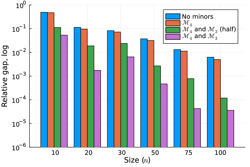
(a) Root node relative gap (rank-1)

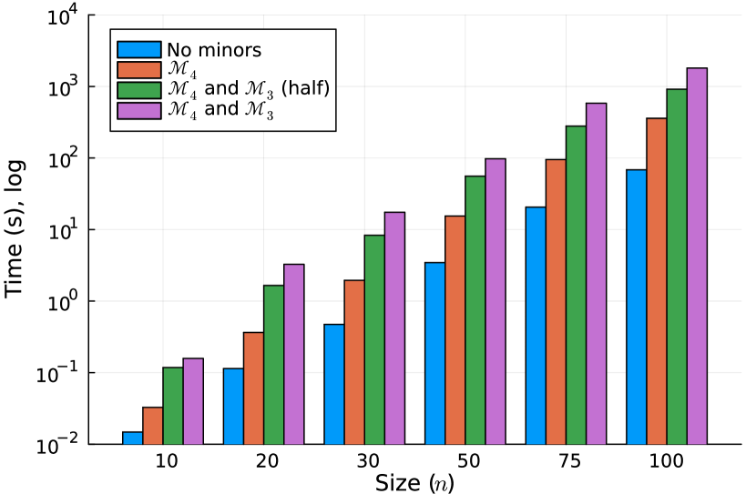
(b) Time taken (rank-1)

Figure 1: Root node relative gap (a) and time taken (b) at the root node for rank-$1$ $n$-by-$n$ matrix completion problems with $2kn\log_{10}(n)$ filled entries, in a regime with low regularization ($\gamma=80.0$).

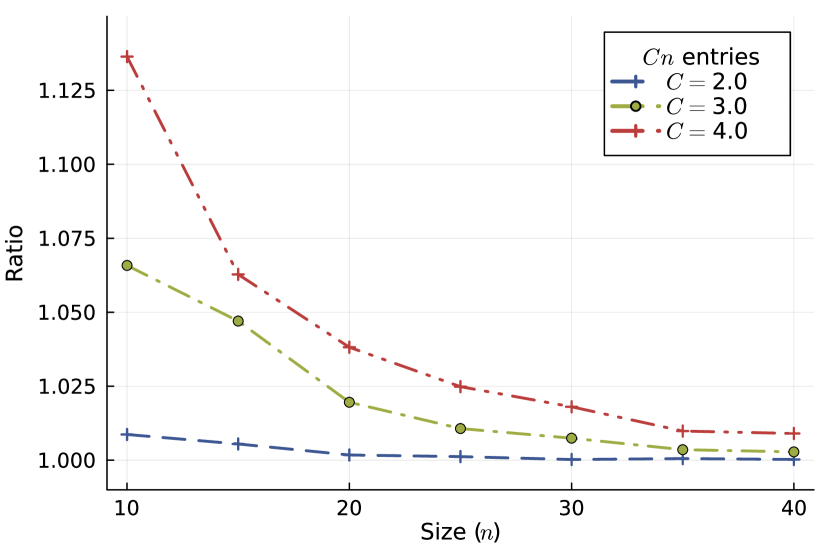
(a) (Scaled) lower bounds of $\mathcal{M}_{4}$ (rank-1)

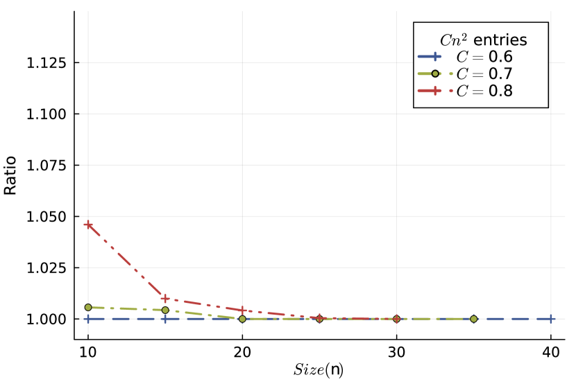
(b) (Scaled) lower bounds of $\mathcal{M}_{4}$ (rank-2)

Figure 2: (Scaled) lower bounds of $\mathcal{M}_{4}$ relaxation relative to the relaxation with no Shor LMIs, with $Cn$ or $Cn^{2}$ entries, with low regularization ($\gamma=80.0$).

5.2.2 Presolving for Basis Pursuit

We now evaluate the efficacy of our presolving strategy for basis pursuit problems, as laid out in Section 3.2. First, we investigate the proportion of entries of an $n\times n$ matrix that our approach fully prescribes. We consider different regimes for $|\mathcal{I}|$. From an information-theoretic perspective, on the order of $kn\log(n)$ entries are necessary for any method to successfully complete a low-rank matrix (Candès and Recht, 2009). Accordingly, we also consider slower and faster rates: $|\mathcal{I}|=p\,k\,r(n)$ with $p=2$ and $r(n)\propto\{n,n\log_{10}(n),n^{6/5}\log_{10}(n),n^{1.5},n^{2}\}$. Figure 3 displays the proportion of random instances that are fully presolved, as $n$ increases. When $|\mathcal{I}|$ grows strictly faster than $n\log_{10}(n)$, more than 90% of instances can be fully presolved when $n\geq 40$, both in the rank-one and rank-two cases, thus demonstrating the effectiveness of our presolving strategy. Moreover, when $|\mathcal{I}|$ is on the order of $n\log_{10}(n)$, the presolving step successfully solves instances where $n$ exceeds $20$, without any optimization.

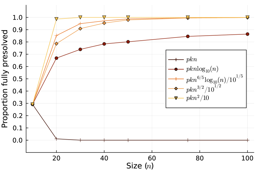
(a) Rank-1

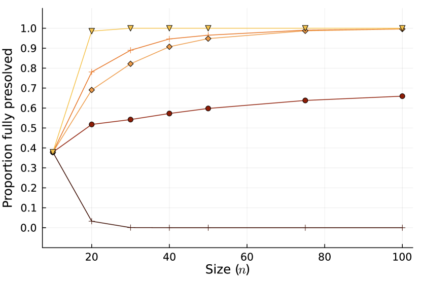
(b) Rank-2

Figure 3: Comparison of proportion of fully presolved instances against problem size $n$ for rank-$k$ ($k\in\{1,2\}$) $n$-by-$n$ basis pursuit problems, varying the number of entries observed initially, where $p=2.0$. Each point is the average of 10,000 random problem instances with the specified parameters.

In addition to reducing the number of variables in our optimization problem, presolving also improves the quality of the matrix perspective relaxation. We now compare the optimality gap at the root node (where we obtain an upper bound by running our branch-and-bound method to optimality on each instance) obtained via different convex relaxations: (i) the original matrix perspective relaxation (8); (ii) the relaxation (i) after presolving the entries belonging to two-by-two minors with three observed entries, $\mathcal{M}_{3}$; (iii) the approach (ii) strengthened by linear equality constraints for the minors with two observed entries, $\mathcal{M}_{2}$; and (iv) the relaxation (iii) further strengthened by Shor LMIs on minors from $\mathcal{M}_{1}$. Results on rank-one basis pursuit problem with $|\mathcal{I}|=pn\log_{10}(n)$ are presented in Figure 4. We observe that presolving alone completely closes the optimality gap, so further strengthening is unnecessary. For example, presolve closes the optimality gap at the root node from $33\%$ for $n=10$, $p=2.0$ to zero.

For rank-two basis pursuit problems, for the problems which we cannot presolve fully, approaches (iii) and (iv) yield instances that are too large for Mosek to solve, even at the root node. Furthermore, approach (ii) followed by our branch-and-bound algorithm runs into out-of-memory errors so, unfortunately, we cannot properly assess the benefits of presolve in yielding tighter relaxations. Overall, for basis pursuit, we observed that presolve yields benefits in relaxation tightness but there is no incremental benefit in relaxation tightness after implementing (iii) and (iv).

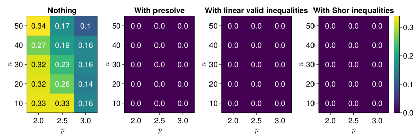
Figure 4: Comparison of relative optimality gap between root-node lower bound and optimal objective for rank-1 basis pursuit problems with $pn\log_{10}(n)$ entries, (i) after implementing presolve, (ii) after also including valid linear inequalities for basis pursuit, (iii) after also including valid Shor inequalities. Each cell is the average (geometric mean) over 20 random instances.

5.3 Branch-and-bound Design Decisions

In this section, we benchmark the efficacy of different algorithmic design options for our branch-and-bound algorithm, including whether to use disjunctive cuts (as developed in Section 2) or a disjunctive scheme based on McCormick inequalities (as described in Section 2.5); the node expansion strategy (breadth-first, best-first, or depth-first); and whether alternating minimization, as described in Section 4.4, should be run at child nodes in the tree.

Tables 1–2 report the final optimality gaps and total computational time of our branch-and-bound scheme with different configurations as we vary $n$. We impose two termination criteria for these experiments: a relative optimality gap $10^{-4}$ and a time limit of one hour. Eigenvector disjunctions achieve optimality gaps about an order of magnitude smaller than McCormick disjunctions. Running alternating minimization at child nodes also improves the average optimality gap by around an order of magnitude, which provides evidence that the Burer-Monteiro alternating minimization method is not optimal in practice when run from the root node, and can be improved via branch-and-bound. Moreover, the best-first node selection strategy, which comprises selecting the unexpanded node with the smallest lower bound at each iteration, outperforms both breadth-first and depth-first search. This phenomenon is consistent across $p$ and $\gamma$; see Tables C.4–C.9. Accordingly, we use best-first search with eigenvector disjunctions and alternating minimization run at child nodes throughout the rest of the paper, unless explicitly indicated otherwise.

We remark that in preliminary numerical experiments, we also considered solving matrix completion problems via the multi-tree branch-and-cut approach proposed in Bertsimas et al. (2022), and directly with Gurobi’s non-convex QCQP solver. Unfortunately, neither approach was competitive with either the McCormick disjunction or the eigenvector disjunction approach, likely because Gurobi does not allow semidefinite constraints to be imposed, and the root node relaxation without semidefinite constraints is often quite weak. Indeed, for instances where $n=50$ and $r>1$, neither approach produced a better lower bound than the matrix perspective relaxation.

$n$	Alternating	Best-first	Breadth-first	Depth-first
	minimization
$10$	✗	$2.37\text{\times}{10}^{-02}$	$3.06\text{\times}{10}^{-02}$	$5.02\text{\times}{10}^{-02}$
$10$	✓	$3.29\text{\times}{10}^{-04}$	$4.90\text{\times}{10}^{-04}$	$7.92\text{\times}{10}^{-03}$
$20$	✗	$4.78\text{\times}{10}^{-03}$	$4.78\text{\times}{10}^{-03}$	$4.78\text{\times}{10}^{-03}$
$20$	✓	$5.51\text{\times}{10}^{-04}$	$8.01\text{\times}{10}^{-04}$	$8.01\text{\times}{10}^{-04}$
$30$	✗	$1.77\text{\times}{10}^{-02}$	$1.77\text{\times}{10}^{-02}$	$1.77\text{\times}{10}^{-02}$
$30$	✓	$2.01\text{\times}{10}^{-03}$	$3.13\text{\times}{10}^{-03}$	$3.13\text{\times}{10}^{-03}$
$40$	✗	$1.32\text{\times}{10}^{-03}$	$1.32\text{\times}{10}^{-03}$	$1.32\text{\times}{10}^{-03}$
$40$	✓	$1.12\text{\times}{10}^{-04}$	$1.12\text{\times}{10}^{-04}$	$1.12\text{\times}{10}^{-04}$
$50$	✗	$6.18\text{\times}{10}^{-04}$	$6.18\text{\times}{10}^{-04}$	$6.18\text{\times}{10}^{-04}$
$50$	✓	$6.37\text{\times}{10}^{-05}$	$6.37\text{\times}{10}^{-05}$	$6.40\text{\times}{10}^{-05}$

(a) Branching with McCormick disjunctions

$n$	Alternating	Best-first	Breadth-first	Depth-first
	minimization
$10$	✗	$5.28\text{\times}{10}^{-03}$	$1.10\text{\times}{10}^{-02}$	$2.60\text{\times}{10}^{-02}$
$10$	✓	2.93e-04	$4.91\text{\times}{10}^{-04}$	$5.22\text{\times}{10}^{-03}$
$20$	✗	$2.61\text{\times}{10}^{-04}$	$4.03\text{\times}{10}^{-04}$	$4.03\text{\times}{10}^{-03}$
$20$	✓	1.32e-04	$1.92\text{\times}{10}^{-04}$	$6.37\text{\times}{10}^{-04}$
$30$	✗	$2.00\text{\times}{10}^{-03}$	$4.16\text{\times}{10}^{-03}$	$1.35\text{\times}{10}^{-02}$
$30$	✓	2.82e-04	$4.53\text{\times}{10}^{-04}$	$1.98\text{\times}{10}^{-03}$
$40$	✗	$3.28\text{\times}{10}^{-04}$	$7.12\text{\times}{10}^{-04}$	$6.11\text{\times}{10}^{-04}$
$40$	✓	1.57e-05	$1.94\text{\times}{10}^{-05}$	$8.25\text{\times}{10}^{-05}$
$50$	✗	$8.11\text{\times}{10}^{-05}$	$3.99\text{\times}{10}^{-04}$	$8.11\text{\times}{10}^{-04}$
$50$	✓	9.99e-06	$1.13\text{\times}{10}^{-05}$	$7.57\text{\times}{10}^{-05}$

(b) Branching with eigenvector disjunctions

Table 1: Final optimality gap across rank-one matrix completion problems with $|\mathcal{I}|=pn\log_{10}(n)$ entries, using McCormick disjunctions (top) and eigenvector disjunctions (bottom), averaged over 20 instances ($p=2.0$, $\gamma=20.0$).

$n$	Alternating	Best-first	Breadth-first	Depth-first
	minimization
$10$	✗	$6.43\text{\times}{10}^{02}$	$6.76\text{\times}{10}^{02}$	$6.94\text{\times}{10}^{02}$
$10$	✓	$1.40\text{\times}{10}^{02}$	$1.36\text{\times}{10}^{02}$	$5.70\text{\times}{10}^{02}$
$20$	✗	$6.93\text{\times}{10}^{02}$	$6.92\text{\times}{10}^{02}$	$6.87\text{\times}{10}^{02}$
$20$	✓	$2.06\text{\times}{10}^{02}$	$2.28\text{\times}{10}^{02}$	$2.37\text{\times}{10}^{02}$
$30$	✗	$3.49\text{\times}{10}^{03}$	$3.49\text{\times}{10}^{03}$	$3.46\text{\times}{10}^{03}$
$30$	✓	$9.21\text{\times}{10}^{02}$	$9.04\text{\times}{10}^{02}$	$9.28\text{\times}{10}^{02}$
$40$	✗	$7.62\text{\times}{10}^{02}$	$7.62\text{\times}{10}^{02}$	$7.66\text{\times}{10}^{02}$
$40$	✓	$5.14\text{\times}{10}^{02}$	$5.08\text{\times}{10}^{02}$	$5.19\text{\times}{10}^{02}$
$50$	✗	$6.51\text{\times}{10}^{02}$	$6.47\text{\times}{10}^{02}$	$6.45\text{\times}{10}^{02}$
$50$	✓	$3.22\text{\times}{10}^{02}$	$3.26\text{\times}{10}^{02}$	$3.26\text{\times}{10}^{02}$

(a) Branching with McCormick disjunctions

$n$	Alternating	Best-first	Breadth-first	Depth-first
	minimization
$10$	✗	$3.10\text{\times}{10}^{02}$	$4.13\text{\times}{10}^{02}$	$8.60\text{\times}{10}^{02}$
$10$	✓	6.37e+01	$1.04\text{\times}{10}^{02}$	$3.98\text{\times}{10}^{02}$
$20$	✗	$2.07\text{\times}{10}^{02}$	$3.46\text{\times}{10}^{02}$	$6.18\text{\times}{10}^{02}$
$20$	✓	5.88e+01	$9.17\text{\times}{10}^{01}$	$2.63\text{\times}{10}^{02}$
$30$	✗	$1.99\text{\times}{10}^{03}$	$2.24\text{\times}{10}^{03}$	$3.38\text{\times}{10}^{03}$
$30$	✓	3.07e+02	$3.35\text{\times}{10}^{02}$	$8.86\text{\times}{10}^{02}$
$40$	✗	$1.83\text{\times}{10}^{02}$	$2.10\text{\times}{10}^{02}$	$7.25\text{\times}{10}^{02}$
$40$	✓	8.19e+01	$9.53\text{\times}{10}^{01}$	$4.99\text{\times}{10}^{02}$
$50$	✗	$3.18\text{\times}{10}^{02}$	$4.56\text{\times}{10}^{02}$	$6.31\text{\times}{10}^{02}$
$50$	✓	1.08e+02	$1.47\text{\times}{10}^{02}$	$4.35\text{\times}{10}^{02}$

(b) Branching with eigenvector disjunctions

Table 2: Computational time (s) across rank-one matrix completion problems with $|\mathcal{I}|=pn\log_{10}(n)$ entries, using McCormick disjunctions (top), eigenvector disjunctions (bottom), averaged over 20 instances ($p=2.0$, $\gamma=20.0$).

We also investigate the effect of the number of pieces in our disjunction, $q$, on the time needed to achieve a $10^{-4}$ optimality gap for rank-one matrix completion problems, in Figure 5. We do not observe a significant difference between using $q=2$ or $q=3$ pieces. However, we find that implementing a disjunctive scheme with $q=4$ pieces allows our branch-and-bound strategy to converge orders of magnitude faster, across all values of $p$ and $\gamma$. We suspect this occurs because four-piece disjunctions include zero as a breakpoint, which breaks some symmetry. However, we also observe that this relative advantage vanishes as $n$ increases; Figure C.4 confirms this on larger instances.

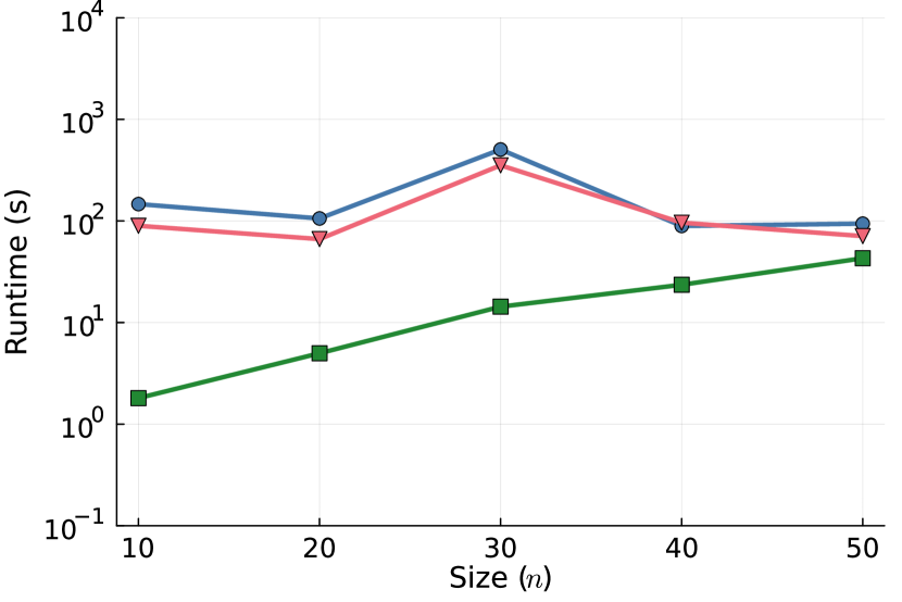
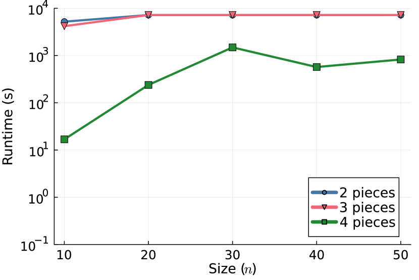
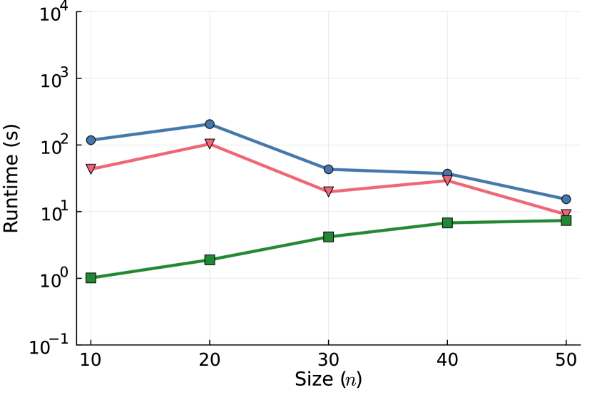
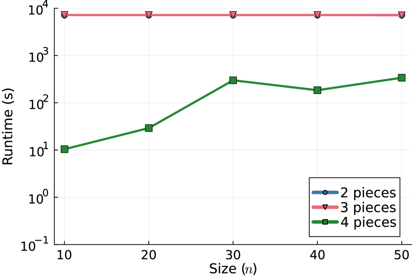
Figure 5: Comparison of time taken to optimality (relative gap $10^{-4}$) for rank-one matrix completion problems with $pn\log_{10}(n)$ filled entries, over different numbers of pieces $q\in\{2,3,4\}$ in upper-approximation. We set $p=2.0$ (less entries) in the top plots, and $p=3.0$ (more entries) in the bottom plots. Moreover, we set $\gamma=20.0$ (more regularization) in the left plots, and $\gamma=80.0$ (less regularization) in the right plots.

5.4 Scalability Experiments

Table 2 reveals that the strongest implementation of our algorithm solves rank-one matrix completion problems where $n=50$ to optimality in minutes. Accordingly, we now investigate the scalability of our algorithm with this configuration, and its ability to obtain higher-quality low-rank matrices than heuristics. We apply our algorithm to rank-$k$ matrix completion problems with $pkn\log_{10}(n)$ entries, $k\in\{1,2,3,4,5\}$, and a time limit of one hour.

Figure 6 depicts the relative gap between the root node relaxation and the best incumbent solution at the root node, and after applying branch-and-bound for one hour.We observe that our branch-and-bound algorithm is highly effective in closing the bounds gap for $k=1$ (when it is most needed); for example, for $k=1$ and $n=10$, branch-and-bound reduces the bound gap from $48\%$ at the root node to $2\%$ after one hour of computational time. As the rank $k$ increases (and, to a lesser extent, as $n$ increases), our algorithm might appear less effective. This behavior can be explained by two factors. First, the root node gap decreases with $k$, providing less room for improvement. For example, from $48\%$ for $n=10$, $k=1$, it drops to $30\%$ for $k=3$ and $4\%$ for $k=5$. Second, the time needed to solve each SDP relaxation increases with $k$, leading to a smaller number of nodes explored within the time limit (see Figure C.5). Nonetheless, our algorithm reduces the optimality gap by 4 percentage points on average, and 5–20 percentage point for the hardest instances.

Figure 7 contrasts the solution found via alternating minimization at the root node against the best solution found by our branch-and-bound scheme after one hour of computational time, as measured by the percentage improvement in mean-squared error on all entries (Figure 8(c) shows the absolute improvement in mean-squared error). We observe that branch-and-bound significantly improves the average relative MSE compared to alternating minimization, with an average relative improvement of more than $50\%$ when $k=2$ and $n\leq 50$, although branch-and-bound’s edge decreases as $n$ increases. This could occur because each semidefinite nodal relaxation is more expensive to solve when $n$ increases, or because there are fewer locally optimal solutions and the landscape of optimal solutions becomes “smoother” as $n$ increases.

Section C.3 augments our comparison of branch-and-bound with the method of Burer and Monteiro (2003), by generating the same plots in different sparsity settings, and comparing our branch-and-bound scheme with a matrix factorization approach using stochastic gradient descent (MFSGD) (Jin et al., 2016). We observe a more significant MSE improvement over MFSGD than over Burer and Monteiro (2003), which can be explained by the fact that MFSGD is designed for scalability rather than accuracy.

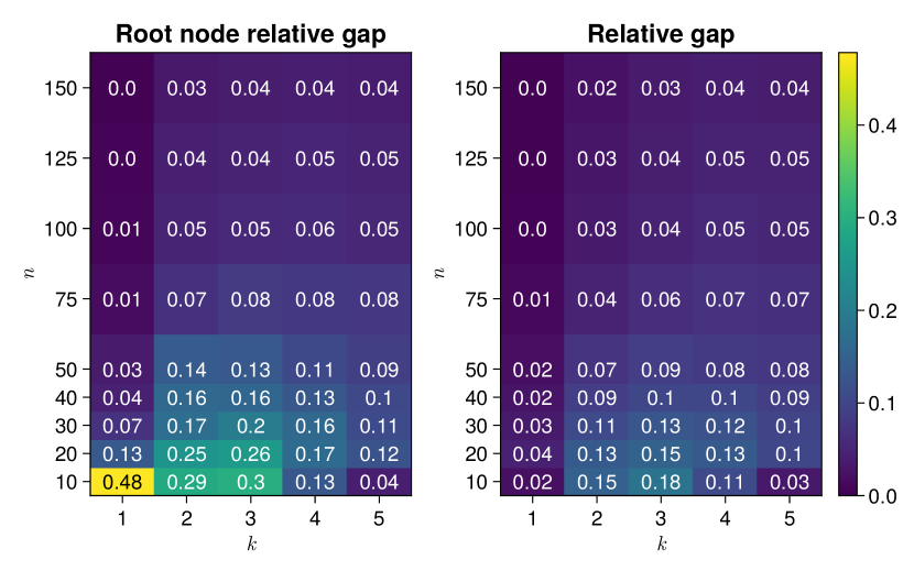
Figure 6: Comparison of relative optimality gap at root node (left) and after running branch-and-bound for one hour (right) for rank-$k$ matrix completion problems with $2kn\log_{10}(n)$ filled entries, varying $n$ and $k$, with $\gamma=80.0$, averaged over 50 instances per point.

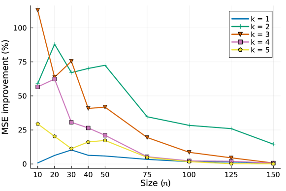
Figure 7: Percentage MSE improvement for rank-$k$ matrix completion problems with $2kn\log_{10}(n)$ filled entries, varying $n$ and $k$, with $\gamma=80.0$, averaged over 50 instances per point.

5.5 Summary of Findings from Numerical Experiments

The main findings from our numerical experiments are as follows:

• Section 5.2 demonstrates that our valid inequalities for matrix completion problems strengthens, often significantly, the semidefinite relaxation (8), and indeed routinely improve the root node gap by an order of magnitude or more in the rank-1 case. However, their efficiency depends on the number of observed entries, especially at larger ranks. Future work could investigate more data-cheap relaxations for the rank $k>1$ cases.

• Section 5.3 investigates the impact of design choices in our branch-and-bound scheme, and demonstrates that eigenvalue-based disjunctions obtain optimality gaps over an order of magnitude smaller than McCormick-based ones in the same amount of computational time.

• Section 5.4 demonstrates that our branch-and-bound scheme solves rank-one matrix completion problems where $n=150$ in minutes or hours, although scalability depends on the rank of the matrix, the amount of data observed and the degree of regularization.

• We observe that, at the information-theoretic threshold identified by Candès and Recht (2009) with $O(nk\log n)$ entries observed, our branch-and-bound scheme obtains low-rank matrices with an out-of-sample predictive power $1\%$–$50\%$ better than solutions obtained via a Burer-Monteiro (BM) heuristic, depending on the rank and the dimensionality of the problem. This can be explained because BM obtains a locally optimal solution which sometimes but not always is globally optimal (see also Ma and Fattahi, 2023, for an investigation of the occasional poor performance of BM).

6 Conclusion

In this paper, we propose a new branch-and-bound scheme for solving low-rank matrix completion and basis pursuit problems to certifiable optimality. The framework considers matrix perspective relaxations and recursively partitions their feasible regions using eigenvector disjunctions. We further strengthen the semidefinite relaxations via preprocessing techniques (for basis pursuit) and valid inequalities (for matrix completion). Existing approaches are either scalable heuristics (but without optimality guarantees), or rely on weak McCormick relaxations and thus cannot scale to $n>50$. On the other hand, our approach successfully scales to solve matrix completion problems over $150\times 150$ matrices and with a rank up to $5$ to certifiable optimality.

Future work could take two future directions. Fist, using eigenvector disjunctions in conjunction with our presolving techniques to improve solution times for other non-convex quadratically constrained problems, such as ACOPF (Kocuk et al., 2016, 2018). Second, integrating eigenvector disjunctions within existing global solvers, either by default or as a viable and potentially more scalable alternative to McCormick branching.

Appendix A Omitted Proofs

A.1 Proof of Proposition 2

Proof

It suffices to show that every feasible solution to Problem (9) can be mapped to a feasible solution to (25) with the same objective value. Therefore, let $(\bm{Y},\bm{U})$ be a feasible solution to Problem (9), let $D=\Set{(i(j),j):j\in[k]}$ denote the set of indices that have been disjuncted on, and select the branch of the disjunction such that $\bm{U}$ satisfies the constraints $U_{i(j),j}\in[\underline{U}_{i(j),j},\overline{U}_{i(j),j}]$ and $U_{i,j}\in[-1,1]$ for all other indices. Then, we need only construct a $\bm{V}$ which satisfies the constraints in (25) to establish the result. To construct such a $\bm{V}$, let us observe that for any $V_{i,j_{1},j_{2}}$, we have constraints on $V_{i,j_{1},j_{2}}$ defined by one of the following four cases:

• If $j:=j_{1}=j_{2}$ and $i\neq i(j)$ then it is not too hard to see that the McCormick constraints reduce to $V_{i,j,j}\in[-1,1]$.

• If $j:=j_{1}=j_{2}$ and $i=i(j)$ then $V_{i,j,j}$ is a subset of $[0,1]$ which contains $U_{i,j}^{2}$.

• If $j_{1}\neq j_{2}$ and $i(j_{1}),i(j_{2})\neq i$ then the McCormick inequalities reduce to $V_{i,j_{1},j_{2}}\in[-1,1]$.

• If $j_{1}\neq j_{2}$ and $i(j_{1})=i$ or $i(j_{2})=i$ then $V_{i,j_{1},j_{2}}$ is a subset of $[-1,1]$ containing $U_{i,j_{1}}U_{i,j_{2}}$.

Recall that $n\geq k+2$. Therefore, we can feasibly set $V_{i(j),j,j}=U_{i(j),j}^{2}$ and $V_{i,j,j}=\frac{1-V_{i(j),j,j}}{n-1}$ for any $i\neq i(j)$. Then, it follows by construction that $\sum_{i=1}^{n}V_{i,j,j}=1$. Moreover, set $V_{i(j_{1}),j_{1},j_{2}}=U_{i(j_{1}),j_{1}}U_{i(j_{1}),j_{2}}$ and $V_{i(j_{2}),j_{1},j_{2}}=U_{i(j_{2}),j_{1}}U_{i(j_{2}),j_{2}}$. Then, since it follows from the $2\times 2$ minors of $\mathbb{I}\succeq\bm{Y}\succeq\bm{U}\bm{U}^{\top}$ that $|\bm{U}_{i}^{\top}\bm{U}_{j}|\leq 1$, we set $V_{i,j_{1},j_{2}}=\frac{-1}{n-k}\left(\sum_{j_{1}=1}^{k}V_{i(j_{2}),j_{1},j_{2}}+\sum_{j_{2}=1}^{k}V_{i(j_{1}),j_{1},j_{2}}\right)$, and it follows by construction that $\sum_{i=1}^{n}V_{i,j_{1},j_{2}}=0$. Therefore, $(\bm{Y},\bm{U},\bm{V})$ is feasible within at least one branch of our disjunction, and there is no single McCormick disjunction which can improve our root node relaxation. ∎

A.2 Proof of Theorem 4.1

Proof

Suppose that at the $L$th iterate this procedure has not converged. Then, since $(\bm{Y}_{L},\bm{U}_{L})$ satisfies the disjunction (24) for any $\bm{x}_{l}$ such that $l<L$, we have that

$$\sum_{t=1}^{k}\langle\bm{x}_{l}^{\top}\bm{U}_{l}^{t},\bm{x}_{l}^{\top}\bm{U}^{t}_{L}\rangle+|(\bm{U}_{l}^{t}-\bm{U}_{L}^{t})^{\top}\bm{x}_{l}|\geq\langle\bm{x}_{l}\bm{x}_{l}^{\top},\bm{Y}_{L}\rangle.$$

But $(\bm{Y}_{l},\bm{U}_{l})$ was not $\epsilon$-feasible, and thus we have that

$$\langle\bm{x}_{l}\bm{x}_{l}^{\top},\bm{Y}_{l}\rangle-\sum_{t=1}^{k}\langle\bm{x}_{l}^{\top}\bm{U}_{l}^{t},\bm{x}_{l}^{\top}\bm{U}^{t}_{l}\rangle>\epsilon.$$

Adding these inequalities then reveals that

$$\langle\bm{x}_{l}\bm{x}_{l}^{\top},\bm{Y}_{l}-\bm{Y}_{L}\rangle+\sum_{t=1}^{k}\langle\bm{x}_{l}^{\top}\bm{U}_{l}^{t},\bm{x}_{l}^{\top}(\bm{U}_{L}^{t}-\bm{U}^{t}_{l})\rangle+\sum_{t=1}^{k}|\bm{x}_{l}^{\top}(\bm{U}_{l}^{t}-\bm{U}^{t}_{L})|>\epsilon.$$

Next, since $|\bm{x}_{l}^{\top}\bm{U}_{l}^{t}|\leq 1$ by construction, using this identity and taking absolute values allows us to conclude that

$$|\langle\bm{x}_{l}\bm{x}_{l}^{\top},\bm{Y}_{l}-\bm{Y}_{L}\rangle|+2\sum_{t=1}^{k}|\bm{x}_{l}^{\top}(\bm{U}_{l}^{t}-\bm{U}^{t}_{L})|>\epsilon.$$

Moreover, by applying the Cauchy-Schwarz inequality to both terms in this inequality we obtain $\langle\bm{x}_{l}\bm{x}_{l}^{\top},\bm{Y}_{l}-\bm{Y}_{L}\rangle\leq\|\bm{Y}_{L}-\bm{Y}_{l}\|_{F}$ and $\sum_{t=1}^{k}|\bm{x}_{l}^{\top}(\bm{U}_{l}^{t}-\bm{U}^{t}_{L})|\leq\sum_{t=1}^{k}\|\bm{U}_{l}^{t}-\bm{U}_{L}^{t}\|_{2}=\|\bm{U}_{l}-\bm{U}_{L}\|_{2,1}$. Further, by norm equivalence we have $\|\bm{U}_{l}-\bm{U}_{L}\|_{2,1}\leq\sqrt{n}\|\bm{U}_{l}-\bm{U}_{L}\|_{F}$. Combining these results allows us to conclude

$$\|\bm{Y}_{l}-\bm{Y}_{L}\|_{F}+2\sqrt{n}\|\bm{U}_{l}-\bm{U}_{L}\|_{F}>\epsilon.$$

That is, with respect to the decision variables $(\bm{Y},\bm{U})$, our procedure never visits any ball of radius $\frac{\epsilon}{2\sqrt{n}}$ twice. Moreover, the set of feasible $(\bm{Y},\bm{U})$ is bounded via $\mathbb{I}\preceq\bm{Y}\preceq\bm{U}\bm{U}^{\top},\mathrm{tr}(\bm{Y})\leq\sqrt{k}$. Therefore, we have that $\|\bm{Y}\|_{F}\leq\sqrt{k}$ and $\|\bm{U}\|_{F}\leq\sqrt{k}$, and thus there are finitely many non-overlapping balls of radius $\frac{\epsilon}{2\sqrt{n}}$ which contain a point in the feasible region. Therefore, for any $\epsilon>0$, our procedure converges within $L(\epsilon)$ iterations for some $L\in\mathbb{N}$. ∎

Appendix B Presolving in Basis Pursuit: Theory and Practice

In this section, we characterize the sparsity patterns of matrices that can arise after presolving in basis pursuit. Recalling that $\mathcal{I}\subset[n]\times[m]$ is the set of indices of observed entries, we define the following index set of presolved entries $\mathcal{I}^{k}$ corresponding to rank-$k$ presolve:

Definition B.1

The index set of presolved entries in rank-$k$ presolve, $\mathcal{I}^{k}$, is constructed from $\mathcal{I}$ by the following procedure:

1. Initialize $\mathcal{I}^{k}\leftarrow\mathcal{I}$.

2. Find sets $R\subset[n]$, $C\subset[m]$, with $|R|=|C|=k+1$, such that $|\mathcal{I}^{k}\cap(R\times C)|=(k+1)^{2}-1$. If no such sets exist, terminate.

3. Update $\mathcal{I}^{k}\leftarrow\mathcal{I}^{k}\cup(R\times C)$ and return to step 2.

For convenience, we define the following sets:

$$\forall\ i\in[n], \mathcal{I}^{k}(i,:) :=\Set{j}{(i,j)\in\mathcal{I}^{k}}$$ (35)

$$\forall\ j\in[m], \mathcal{I}^{k}(:,j) :=\Set{i}{(i,j)\in\mathcal{I}^{k}}$$ (36)

$$\forall\ R\subset[n], \mathcal{I}^{k}(R,:) :=\Set{j}{(i,j)\in\mathcal{I}^{k}\ \forall\ i\in R}=\bigcap_{i\in R}\mathcal{I}^{k}(i,:)$$ (37)

$$\forall\ C\subset[m], \mathcal{I}^{k}(:,C) :=\Set{j}{(i,j)\in\mathcal{I}^{k}\ \forall\ j\in C}=\bigcap_{j\in C}\mathcal{I}^{k}(:,j)$$ (38)

In the rank-1 case, we have the following result:

Lemma B.1

$\mathcal{I}^{1}$ satisfies the following properties:

• For any $i_{1},i_{2}\in[n]$, either $\mathcal{I}^{1}(i_{1},:)=\mathcal{I}^{1}(i_{2},:)$ or $\lvert\mathcal{I}^{k}(\{i_{1},i_{2}\},:)\rvert=0$.

• For any $j_{1},j_{2}\in[m]$, either $\mathcal{I}^{1}(:,j_{1})=\mathcal{I}^{1}(:,j_{2})$ or $\lvert\mathcal{I}^{k}(:,\{j_{1},j_{2}\})\rvert=0$.

This implies that $\mathcal{I}^{1}$ can be expressed as:

$$\mathcal{I}^{1}=(R_{1}\times C_{1})\cup(R_{2}\times C_{2})\cup\dots,$$ (39)

where $\{R_{i}\}$ are nonempty and form a partition of $[n]$, and $C_{j}$ are nonempty and form a partition of $[m]$. Intuitively, there exists a permutation of the rows and columns of the matrix such that $\mathcal{I}^{1}$ has a “block-rectangular” structure.

In the general rank-$k$ case, we have the following extension:

Lemma B.2

$\mathcal{I}^{k}$ satisfies the following properties:

• For $R_{1},R_{2}\subset[n]$ with $|R_{1}|=|R_{2}|=k$, either $\mathcal{I}^{k}(R_{1},:)=\mathcal{I}^{k}(R_{2},:)$ or $\lvert\mathcal{I}^{k}(R_{1}\cap R_{2},:)\rvert<k$.

• For $C_{1},C_{2}\subset[m]$ with $|C_{1}|=|C_{2}|=k$, either $\mathcal{I}^{k}(:,C_{1})=\mathcal{I}^{k}(:,C_{2})$ or $\lvert\mathcal{I}^{k}(:,C_{1}\cap C_{2})\rvert<k$.

Proof

We prove the first property (the second is symmetrical). Suppose $R_{1}\neq R_{2}$ (which implies $|R_{1}\cup R_{2}|\geq k+1$). (If $R_{1}=R_{2}$ then ${\mathcal{I}^{1}(R_{1},:)}={\mathcal{I}^{1}(R_{2},:)}$ and we are done.) Also suppose that ${\mathcal{I}^{1}(R_{1}\cap R_{2},:)}\geq k$. Then there exists $k$ column indices $C=\{j_{1},j_{2},\dots,j_{k}\}$ such that $C\subset\mathcal{I}^{1}(R_{1}\cap R_{2},:)$, i.e. $(R_{1}\cup R_{2})\times C\subset\mathcal{I}^{k}$.

Suppose for the sake of contradiction that there exists $j\in\mathcal{I}^{1}(R_{1},:)\setminus\mathcal{I}^{1}(R_{2},:)$ (the case where $\lvert\mathcal{I}^{1}(R_{2},:)\setminus\mathcal{I}^{1}(R_{1},:)\rvert>0$ is identical). Select $i\in R_{2}\setminus R_{1}$. Then, the $k$ indices in $\{i\}\times C$ and the $k(k+1)$ indices in $R_{1}\times(C\cup\{j\})$ all belong in $\mathcal{I}$, and therefore $(R_{1}\cup\{i\})\times(C\cup\{j\})$ defines a $(k+1)$-by-$(k+1)$ minor with $(k+1)^{2}-1$ observed entries. This means that $(i,j)$ could still be added as a presolved entry to $\mathcal{I}^{k}$, which contradicts the definition of $\mathcal{I}^{k}$. ∎

In a practical implementation of the presolve stage for rank-$k$ basis pursuit stage, we perform the procedure described in Definition B.1. Instead of enumerating all ${n\choose k+1}\times{m\choose k+1}$ possibilities for $R$ and $C$ in step 2, which is prohibitively expensive, we use Lemma B.2 to reduce the number of row-sets and column-sets to search over. The observation is that if $R\times C$ has $(k+1)^{2}-1$ entries in $\mathcal{I}^{k}$, then there must exist $C^{\prime}\subset C$ ($R^{\prime}\subset R$) with $|C^{\prime}|=k$ ($|R^{\prime}|=k$) respectively such that $R^{\prime}\times C$ and $R\times C^{\prime}$ are in $\mathcal{I}^{k}$. In particular, $\mathcal{I}^{k}(:,C^{\prime})\geq(k+1)$, and we use this in line 5 of Algorithm 2. Also, $|R^{\prime}|=k$ implies that the set $\overline{R}:=\{r\in\mathcal{I}^{k}(:,C^{\prime}):(r,j)\in\mathcal{I}^{k}\}$ must satisfy $|\overline{R}|\geq k$; we use this in line 8 of Algorithm 2 to accelerate the algorithm. These accelerations perform better in a sparser regime, because many row-sets and column-sets can be skipped.

Algorithm 2 Presolve for rank-$k$ basis pursuit problems

1:Initialize $\mathcal{I}^{k}=\mathcal{I}$;

2:while not converged do

3:     converged $\leftarrow\texttt{true}$;

4:     for each $C^{\prime}\subset[m]$ with $|C^{\prime}|=k$ do

5:         if $|\mathcal{I}^{k}(:,C^{\prime})|\leq k$, continue;

6:         for $j\in[m]\setminus C^{\prime}$ do

7:              Define $C:=C^{\prime}\cup\{j\}$;

8:              Define $\overline{R}:=\{r\in\mathcal{I}^{k}(:,C^{\prime}):(r,j)\in\mathcal{I}^{k}\}$ (if $|\overline{R}|<k$, continue);

9:              Choose $R^{\prime}\subset\overline{R}$ such that $|R^{\prime}|=k$;

10:              for $i\in\mathcal{I}^{k}(:,C^{\prime})\setminus\overline{R}$ do

11:                  Define $R:=R^{\prime}\cup\{i\}$;

12:                  Update $\mathcal{I}^{k}\leftarrow\mathcal{I}^{k}\cup(R\times C)$ and set converged $\leftarrow\texttt{false}$;

13:                  Presolve $(i,j)$ based on other entries in $R\times C$;

14:              end for

15:         end for

16:     end for

17:end while

18:return $\mathcal{I}^{k}$

Appendix C Numerical results

C.1 Root Node: Strengthened Relaxations and Presolving

Figure C.1 and Tables C.1–C.2 illustrate the trade-off between optimality gap at the root node (the upper bound is obtained via alternating minimization) and computational time, for solving the strengthened relaxation in rank-1 matrix completion. Observe that imposing more Shor LMIs yields tighter but (potentially significantly) more computationally expensive semidefinite relaxations across all sizes, regularization parameters, and sparsity settings. Moreover, imposing constraints on all minors in $\mathcal{M}_{4}$ and $\mathcal{M}_{3}$ (as compared to just those in $\mathcal{M}_{4}$) leads to a larger reduction in optimality gap when $\gamma=80.0$ (1–3 orders of magnitude) than when $\gamma=20.0$ (0–2 orders of magnitude). Therefore, the benefits from our strengthened relaxation appear more salient in regimes with less regularization.

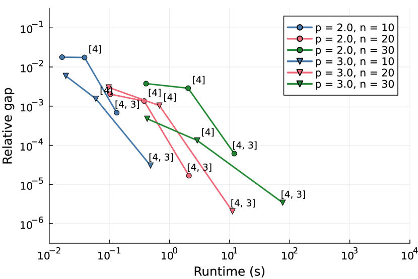
(a) small instances, $\gamma=20.0$: more regularized

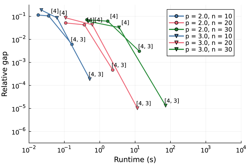
(b) small instances, $\gamma=80.0$: less regularized

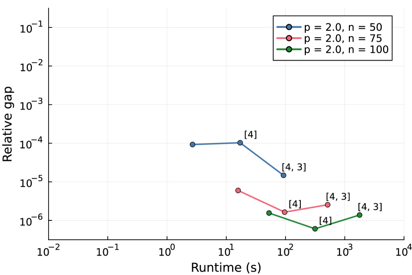
(c) larger instances, $\gamma=20.0$: more regularized

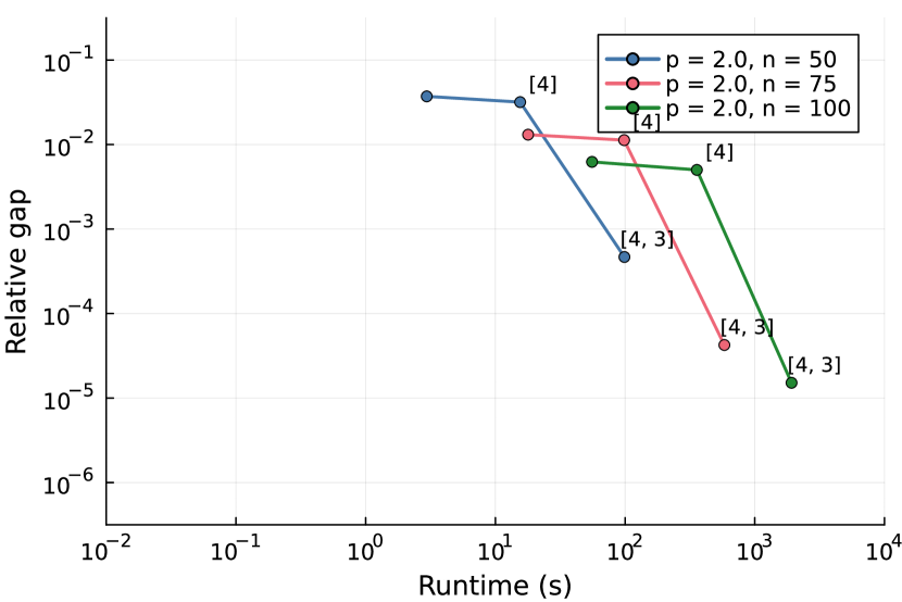
(d) larger instances, $\gamma=80.0$: less regularized

Figure C.1: Comparison of relative bound gap at the root node against time for the root node relaxations of rank-1 matrix completion problems, varying the number and kind of Shor LMIs added. Each point is the average (geometric mean) of 20 random problem instances with the specified parameters.

			Root node gap
$n$	$p$	$\gamma$	None	Shor(4)	Shor(4, 3)
$10$	$2.0$	$20.0$	$0.0163$	$0.0386$	$0.132$
		$80.0$	$0.0182$	$0.0359$	$0.164$
	$3.0$	$20.0$	$0.0189$	$0.0596$	$0.484$
		$80.0$	$0.0224$	$0.062$	$0.523$
$20$	$2.0$	$20.0$	$0.104$	$0.379$	$2.11$
		$80.0$	$0.109$	$0.368$	$2.33$
	$3.0$	$20.0$	$0.0976$	$0.68$	$11.2$
		$80.0$	$0.109$	$0.615$	$11.6$
$30$	$2.0$	$20.0$	$0.408$	$2.05$	$12.0$
		$80.0$	$0.435$	$1.69$	$13.2$
	$3.0$	$20.0$	$0.426$	$2.9$	$76.6$
		$80.0$	$0.475$	$3.54$	$72.9$

Table C.1: Time taken at root node across rank-one matrix completion problems with $pkn\log_{10}(n)$ filled entries, with different Shor LMIs added (averaged over 20 instances per row).

			Root node gap
$n$	$p$	$\gamma$	None	Shor(4)	Shor(4, 3)
$10$	$2.0$	$20.0$	$1.78\text{\times}{10}^{-2}$	$1.75\text{\times}{10}^{-2}$	$6.81\text{\times}{10}^{-4}$
		$80.0$	$1.14\text{\times}{10}^{-1}$	$1.05\text{\times}{10}^{-1}$	$6.09\text{\times}{10}^{-3}$
	$3.0$	$20.0$	$5.93\text{\times}{10}^{-3}$	$1.54\text{\times}{10}^{-3}$	$3.04\text{\times}{10}^{-5}$
		$80.0$	$1.88\text{\times}{10}^{-1}$	$8.62\text{\times}{10}^{-2}$	$1.87\text{\times}{10}^{-4}$
$20$	$2.0$	$20.0$	$2.02\text{\times}{10}^{-3}$	$1.35\text{\times}{10}^{-3}$	$1.68\text{\times}{10}^{-5}$
		$80.0$	$5.17\text{\times}{10}^{-2}$	$4.31\text{\times}{10}^{-2}$	$4.69\text{\times}{10}^{-4}$
	$3.0$	$20.0$	$3.01\text{\times}{10}^{-3}$	$1.04\text{\times}{10}^{-3}$	$2.06\text{\times}{10}^{-6}$
		$80.0$	$8.67\text{\times}{10}^{-2}$	$4.33\text{\times}{10}^{-2}$	$1.02\text{\times}{10}^{-5}$
$30$	$2.0$	$20.0$	$3.76\text{\times}{10}^{-3}$	$2.88\text{\times}{10}^{-3}$	$6.15\text{\times}{10}^{-5}$
		$80.0$	$7.10\text{\times}{10}^{-2}$	$6.18\text{\times}{10}^{-2}$	$3.06\text{\times}{10}^{-3}$
	$3.0$	$20.0$	$4.77\text{\times}{10}^{-4}$	$1.33\text{\times}{10}^{-4}$	$3.42\text{\times}{10}^{-6}$
		$80.0$	$6.08\text{\times}{10}^{-2}$	$3.29\text{\times}{10}^{-2}$	$1.32\text{\times}{10}^{-5}$

Table C.2: Relative gap at the root node across rank-one matrix completion problems with $pkn\log_{10}(n)$ filled entries, with different Shor LMIs added (averaged over 20 instances per row)

Notably, while including different types of minors ($\mathcal{M}_{4}$ and $\mathcal{M}_{3}$ instead of just $\mathcal{M}_{4}$) provides a way to control the trade-off between computation time and relaxation strength, this can also be done by including a subset of minors in $\mathcal{M}_{4}\cup\mathcal{M}_{3}$. This is most clearly seen in Figure C.2, where either half or all of the minors in $\mathcal{M}_{4}\cup\mathcal{M}_{3}$ are imposed. The merits of either approach differ based on sparsity (number of filled entries) and problem size. Unfortunately, we do not observe a strengthened relaxation in the rank-2 case despite imposing constraints on more minors, as demonstrated in Figure C.3 and C.3.

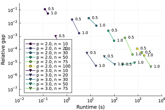
Figure C.2: Comparison of relative bound gap at the root node against time for the root node relaxations of rank-1 matrix completion problems, varying the proportion of Shor LMIs added ($\gamma=80.0$).

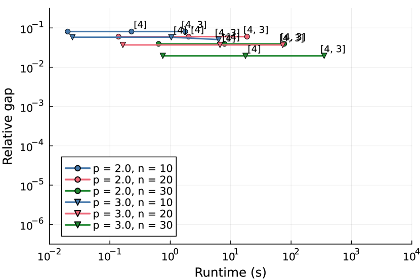
(a) small instances, $\gamma=20.0$: more regularized

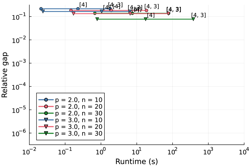
(b) small instances, $\gamma=80.0$: less regularized

Figure C.3: Comparison of relative bound gap at the root node against time for the root node relaxations of rank-2 matrix completion problems, varying the number and kind of Shor LMIs added. Each point is the average (geometric mean) of 20 random problem instances with the specified parameters.

			Time taken (s)			Root node gap
$n$	$p$	$\gamma$	None	$\mathcal{M}_{4}$	$\mathcal{M}_{4}\cup\mathcal{M}_{3}$	None	$\mathcal{M}_{4}$	$\mathcal{M}_{4}\cup\mathcal{M}_{3}$
$10$	$2.0$	$20.0$	$0.0200$	$0.228$	$1.77$	$0.081$	$0.081$	$0.081$
		$80.0$	$0.0212$	$0.228$	$1.81$	$0.216$	$0.216$	$0.216$
	$3.0$	$20.0$	$0.0240$	$1.04$	$6.32$	$0.0581$	$0.0581$	$0.0506$
		$80.0$	$0.0240$	$1.05$	$6.43$	$0.165$	$0.165$	$0.165$
$20$	$2.0$	$20.0$	$0.139$	$2.01$	$18.7$	$0.0601$	$0.0601$	$0.0601$
		$80.0$	$0.145$	$1.94$	$18.7$	$0.183$	$0.183$	$0.183$
	$3.0$	$20.0$	$0.164$	$6.65$	$72.9$	$0.0369$	$0.0369$	$0.0369$
		$80.0$	$0.171$	$6.54$	$76.7$	$0.133$	$0.133$	$0.133$
$30$	$2.0$	$20.0$	$0.640$	$7.91$	$77.2$	$0.0394$	$0.0394$	$0.0394$
		$80.0$	$0.675$	$7.55$	$77.6$	$0.138$	$0.138$	$0.138$
	$3.0$	$20.0$	$0.752$	$17.6$	$353$	$0.0195$	$0.0195$	$0.0195$
		$80.0$	$0.784$	$17.7$	$381$	$0.0772$	$0.0772$	$0.0772$

Table C.3: Comparing time taken and relative gap at the root node across rank-two matrix completion problems with $pkn\log_{10}(n)$ filled entries, with different Shor LMIs added (averaged over 20 instances per row)

C.2 Branch-and-bound Design Decisions

In this section, we document the performance of our branch-and-bound scheme with various parameter settings: comparing our eigenvalue disjunctions to a naive McCormick-based approach, changing the order of the nodes explored, and including alternating minimization at child nodes of the search tree. We evaluate all combinations of parameter settings, and record their relative optimality gap and time taken (capped at 1 hour) for rank-1 matrix completion problems with regularization $\gamma\in\{20.0,80.0\}$ and $pn\log_{10}(n)$ filled entries with $p\in\{2.0,3.0\}$. The results are shown in Tables 1–2, C.4–C.5 (less entries $p=2.0$ and less regularization $\gamma=80.0$), C.6–C.7 (more entries $p=3.0$ and more regularization $\gamma=20.0$), and C.8–C.9 (more entries $p=3.0$ and less regularization $\gamma=80.0$) respectively.

The tables show that eigenvector disjunctions perform consistently better than McCormick disjunctions, and that best-first search on unexplored child nodes is usually a good node selection strategy. They also illustrate the power of performing alternating minimization at (some) child nodes, because better feasible solutions can be found with different initializations, which yield tight upper bounds and thereby accelerating the branch-and-bound procedure.

$n$	Alternating	Best-first	Breadth-first	Depth-first
	minimization
$10$	✗	$2.56\text{\times}{10}^{-01}$	$3.21\text{\times}{10}^{-01}$	$3.75\text{\times}{10}^{-01}$
$10$	✓	1.44e-02	$2.71\text{\times}{10}^{-02}$	$1.12\text{\times}{10}^{-01}$
$20$	✗	$1.09\text{\times}{10}^{-01}$	$1.09\text{\times}{10}^{-01}$	$1.09\text{\times}{10}^{-01}$
$20$	✓	$5.88\text{\times}{10}^{-02}$	$6.05\text{\times}{10}^{-02}$	$6.06\text{\times}{10}^{-02}$
$30$	✗	$1.31\text{\times}{10}^{-01}$	$1.31\text{\times}{10}^{-01}$	$1.31\text{\times}{10}^{-01}$
$30$	✓	$6.94\text{\times}{10}^{-02}$	$7.08\text{\times}{10}^{-02}$	$7.08\text{\times}{10}^{-02}$
$40$	✗	$7.76\text{\times}{10}^{-02}$	$7.76\text{\times}{10}^{-02}$	$7.76\text{\times}{10}^{-02}$
$40$	✓	$4.27\text{\times}{10}^{-02}$	$4.27\text{\times}{10}^{-02}$	$4.27\text{\times}{10}^{-02}$
$50$	✗	$3.71\text{\times}{10}^{-02}$	$3.71\text{\times}{10}^{-02}$	$3.71\text{\times}{10}^{-02}$
$50$	✓	$2.55\text{\times}{10}^{-02}$	$2.55\text{\times}{10}^{-02}$	$2.55\text{\times}{10}^{-02}$

(a) Branching with McCormick disjunctions

$n$	Alternating	Best-first	Breadth-first	Depth-first
	minimization
$10$	✗	$3.19\text{\times}{10}^{-01}$	$3.93\text{\times}{10}^{-01}$	$4.73\text{\times}{10}^{-01}$
$10$	✓	$1.48\text{\times}{10}^{-02}$	$2.63\text{\times}{10}^{-02}$	$9.37\text{\times}{10}^{-02}$
$20$	✗	$1.12\text{\times}{10}^{-01}$	$1.34\text{\times}{10}^{-01}$	$1.39\text{\times}{10}^{-01}$
$20$	✓	3.53e-02	$4.64\text{\times}{10}^{-02}$	$1.10\text{\times}{10}^{-01}$
$30$	✗	$1.34\text{\times}{10}^{-01}$	$1.45\text{\times}{10}^{-01}$	$1.48\text{\times}{10}^{-01}$
$30$	✓	3.60e-02	$4.27\text{\times}{10}^{-02}$	$6.76\text{\times}{10}^{-02}$
$40$	✗	$6.77\text{\times}{10}^{-02}$	$7.38\text{\times}{10}^{-02}$	$7.93\text{\times}{10}^{-02}$
$40$	✓	2.27e-02	$2.58\text{\times}{10}^{-02}$	$4.16\text{\times}{10}^{-02}$
$50$	✗	$4.85\text{\times}{10}^{-02}$	$5.15\text{\times}{10}^{-02}$	$5.41\text{\times}{10}^{-02}$
$50$	✓	1.66e-02	$1.83\text{\times}{10}^{-02}$	$2.98\text{\times}{10}^{-02}$

(b) Branching with eigenvector disjunctions

Table C.4: Final optimality gap across rank-one matrix completion problems with $|\mathcal{I}|=pn\log_{10}(n)$ entries, using McCormick disjunctions (top) and eigenvector disjunctions (bottom), averaged over 20 instances ($p=2.0$, $\gamma=80.0$).

$n$	Alternating	Best-first	Breadth-first	Depth-first
	minimization
$10$	✗	$1.86\text{\times}{10}^{03}$	$2.08\text{\times}{10}^{03}$	$2.12\text{\times}{10}^{03}$
$10$	✓	1.40e+03	$1.55\text{\times}{10}^{03}$	$2.18\text{\times}{10}^{03}$
$20$	✗	$3.25\text{\times}{10}^{03}$	$3.27\text{\times}{10}^{03}$	$3.21\text{\times}{10}^{03}$
$20$	✓	$2.89\text{\times}{10}^{03}$	$2.78\text{\times}{10}^{03}$	$3.16\text{\times}{10}^{03}$
$30$	✗	$3.49\text{\times}{10}^{03}$	$3.48\text{\times}{10}^{03}$	$3.46\text{\times}{10}^{03}$
$30$	✓	$3.38\text{\times}{10}^{03}$	$3.26\text{\times}{10}^{03}$	$3.45\text{\times}{10}^{03}$
$40$	✗	$3.54\text{\times}{10}^{03}$	$3.54\text{\times}{10}^{03}$	$3.53\text{\times}{10}^{03}$
$40$	✓	$3.48\text{\times}{10}^{03}$	$3.41\text{\times}{10}^{03}$	$3.53\text{\times}{10}^{03}$
$50$	✗	$3.56\text{\times}{10}^{03}$	$3.56\text{\times}{10}^{03}$	$3.56\text{\times}{10}^{03}$
$50$	✓	$3.50\text{\times}{10}^{03}$	$3.46\text{\times}{10}^{03}$	$3.55\text{\times}{10}^{03}$

(a) Branching with McCormick disjunctions

$n$	Alternating	Best-first	Breadth-first	Depth-first
	minimization
$10$	✗	$2.40\text{\times}{10}^{03}$	$2.74\text{\times}{10}^{03}$	$2.88\text{\times}{10}^{03}$
$10$	✓	$1.68\text{\times}{10}^{03}$	$2.10\text{\times}{10}^{03}$	$2.73\text{\times}{10}^{03}$
$20$	✗	$3.22\text{\times}{10}^{03}$	$3.24\text{\times}{10}^{03}$	$3.21\text{\times}{10}^{03}$
$20$	✓	$2.64\text{\times}{10}^{03}$	2.49e+03	$3.07\text{\times}{10}^{03}$
$30$	✗	$3.40\text{\times}{10}^{03}$	$3.42\text{\times}{10}^{03}$	$3.39\text{\times}{10}^{03}$
$30$	✓	$2.97\text{\times}{10}^{03}$	2.89e+03	$3.28\text{\times}{10}^{03}$
$40$	✗	$3.49\text{\times}{10}^{03}$	$3.50\text{\times}{10}^{03}$	$3.46\text{\times}{10}^{03}$
$40$	✓	$3.22\text{\times}{10}^{03}$	3.18e+03	$3.42\text{\times}{10}^{03}$
$50$	✗	$3.54\text{\times}{10}^{03}$	$3.54\text{\times}{10}^{03}$	$3.52\text{\times}{10}^{03}$
$50$	✓	$3.36\text{\times}{10}^{03}$	3.34e+03	$3.48\text{\times}{10}^{03}$

(b) Branching with eigenvector disjunctions

Table C.5: Computational time (s) across rank-one matrix completion problems with $|\mathcal{I}|=pn\log_{10}(n)$ entries, using McCormick disjunctions (top), eigenvector disjunctions (bottom), averaged over 20 instances ($p=2.0$, $\gamma=80.0$).

$n$	Alternating	Best-first	Breadth-first	Depth-first
	minimization
$10$	✗	$7.61\text{\times}{10}^{-03}$	$8.77\text{\times}{10}^{-03}$	$1.64\text{\times}{10}^{-02}$
$10$	✓	$6.27\text{\times}{10}^{-04}$	$7.68\text{\times}{10}^{-04}$	$6.26\text{\times}{10}^{-03}$
$20$	✗	$6.96\text{\times}{10}^{-03}$	$6.96\text{\times}{10}^{-03}$	$6.96\text{\times}{10}^{-03}$
$20$	✓	$6.22\text{\times}{10}^{-04}$	$1.67\text{\times}{10}^{-03}$	$1.67\text{\times}{10}^{-03}$
$30$	✗	$3.31\text{\times}{10}^{-03}$	$3.31\text{\times}{10}^{-03}$	$3.31\text{\times}{10}^{-03}$
$30$	✓	$1.05\text{\times}{10}^{-04}$	$2.37\text{\times}{10}^{-04}$	$2.37\text{\times}{10}^{-04}$
$40$	✗	$1.78\text{\times}{10}^{-04}$	$1.78\text{\times}{10}^{-04}$	$1.78\text{\times}{10}^{-04}$
$40$	✓	$5.86\text{\times}{10}^{-05}$	$5.86\text{\times}{10}^{-05}$	$5.86\text{\times}{10}^{-05}$
$50$	✗	$6.46\text{\times}{10}^{-05}$	$6.46\text{\times}{10}^{-05}$	$6.46\text{\times}{10}^{-05}$
$50$	✓	$2.24\text{\times}{10}^{-06}$	$2.24\text{\times}{10}^{-06}$	$2.24\text{\times}{10}^{-06}$

(a) Branching with McCormick disjunctions

$n$	Alternating	Best-first	Breadth-first	Depth-first
	minimization
$10$	✗	$9.09\text{\times}{10}^{-04}$	$1.21\text{\times}{10}^{-03}$	$1.42\text{\times}{10}^{-02}$
$10$	✓	1.28e-04	$2.08\text{\times}{10}^{-04}$	$3.69\text{\times}{10}^{-03}$
$20$	✗	$6.23\text{\times}{10}^{-05}$	$3.12\text{\times}{10}^{-04}$	$8.24\text{\times}{10}^{-04}$
$20$	✓	8.14e-05	$1.40\text{\times}{10}^{-04}$	$7.20\text{\times}{10}^{-04}$
$30$	✗	$9.04\text{\times}{10}^{-05}$	$3.05\text{\times}{10}^{-04}$	$1.04\text{\times}{10}^{-03}$
$30$	✓	1.60e-05	$2.25\text{\times}{10}^{-05}$	$6.00\text{\times}{10}^{-05}$
$40$	✗	$2.16\text{\times}{10}^{-05}$	$3.41\text{\times}{10}^{-05}$	$1.39\text{\times}{10}^{-04}$
$40$	✓	4.97e-06	$5.30\text{\times}{10}^{-06}$	$3.20\text{\times}{10}^{-05}$
$50$	✗	3.86e-07	$1.47\text{\times}{10}^{-06}$	$2.58\text{\times}{10}^{-06}$
$50$	✓	$1.02\text{\times}{10}^{-06}$	$1.04\text{\times}{10}^{-06}$	$4.09\text{\times}{10}^{-07}$

(b) Branching with eigenvector disjunctions

Table C.6: Final optimality gap across rank-one matrix completion problems with $|\mathcal{I}|=pn\log_{10}(n)$ entries, using McCormick disjunctions (top) and eigenvector disjunctions (bottom), averaged over 20 instances ($p=3.0$, $\gamma=20.0$).

$n$	Alternating	Best-first	Breadth-first	Depth-first
	minimization
$10$	✗	$2.48\text{\times}{10}^{02}$	$2.76\text{\times}{10}^{02}$	$3.77\text{\times}{10}^{02}$
$10$	✓	$1.26\text{\times}{10}^{02}$	$1.46\text{\times}{10}^{02}$	$3.90\text{\times}{10}^{02}$
$20$	✗	$1.19\text{\times}{10}^{03}$	$1.19\text{\times}{10}^{03}$	$1.17\text{\times}{10}^{03}$
$20$	✓	$4.35\text{\times}{10}^{02}$	$6.66\text{\times}{10}^{02}$	$6.85\text{\times}{10}^{02}$
$30$	✗	$9.20\text{\times}{10}^{02}$	$9.26\text{\times}{10}^{02}$	$9.17\text{\times}{10}^{02}$
$30$	✓	$3.48\text{\times}{10}^{02}$	$3.74\text{\times}{10}^{02}$	$3.75\text{\times}{10}^{02}$
$40$	✗	$1.08\text{\times}{10}^{02}$	$1.08\text{\times}{10}^{02}$	$1.08\text{\times}{10}^{02}$
$40$	✓	$1.10\text{\times}{10}^{02}$	$1.07\text{\times}{10}^{02}$	$1.08\text{\times}{10}^{02}$
$50$	✗	$1.73\text{\times}{10}^{02}$	$1.72\text{\times}{10}^{02}$	$1.71\text{\times}{10}^{02}$
$50$	✓	$6.23\text{\times}{10}^{01}$	$6.20\text{\times}{10}^{01}$	$6.21\text{\times}{10}^{01}$

(a) Branching with McCormick disjunctions

$n$	Alternating	Best-first	Breadth-first	Depth-first
	minimization
$10$	✗	$1.27\text{\times}{10}^{02}$	$1.75\text{\times}{10}^{02}$	$4.71\text{\times}{10}^{02}$
$10$	✓	5.65e+01	$1.10\text{\times}{10}^{02}$	$3.87\text{\times}{10}^{02}$
$20$	✗	$1.53\text{\times}{10}^{02}$	$2.55\text{\times}{10}^{02}$	$4.41\text{\times}{10}^{02}$
$20$	✓	1.30e+02	$2.01\text{\times}{10}^{02}$	$4.15\text{\times}{10}^{02}$
$30$	✗	$6.42\text{\times}{10}^{01}$	$8.55\text{\times}{10}^{01}$	$5.89\text{\times}{10}^{02}$
$30$	✓	3.31e+01	$5.51\text{\times}{10}^{01}$	$1.60\text{\times}{10}^{02}$
$40$	✗	$5.45\text{\times}{10}^{01}$	$7.93\text{\times}{10}^{01}$	$1.07\text{\times}{10}^{02}$
$40$	✓	3.19e+01	$4.79\text{\times}{10}^{01}$	$1.08\text{\times}{10}^{02}$
$50$	✗	$1.56\text{\times}{10}^{01}$	$1.90\text{\times}{10}^{01}$	$5.12\text{\times}{10}^{01}$
$50$	✓	1.33e+01	$1.50\text{\times}{10}^{01}$	$3.68\text{\times}{10}^{01}$

(b) Branching with eigenvector disjunctions

Table C.7: Computational time (s) across rank-one matrix completion problems with $|\mathcal{I}|=pn\log_{10}(n)$ entries, using McCormick disjunctions (top), eigenvector disjunctions (bottom), averaged over 20 instances ($p=3.0$, $\gamma=20.0$).

$n$	Alternating	Best-first	Breadth-first	Depth-first
	minimization
$10$	✗	$1.44\text{\times}{10}^{-01}$	$1.85\text{\times}{10}^{-01}$	$3.45\text{\times}{10}^{-01}$
$10$	✓	2.97e-02	$5.86\text{\times}{10}^{-02}$	$1.88\text{\times}{10}^{-01}$
$20$	✗	$1.29\text{\times}{10}^{-01}$	$1.29\text{\times}{10}^{-01}$	$1.29\text{\times}{10}^{-01}$
$20$	✓	$6.74\text{\times}{10}^{-02}$	$9.05\text{\times}{10}^{-02}$	$9.05\text{\times}{10}^{-02}$
$30$	✗	$1.03\text{\times}{10}^{-01}$	$1.03\text{\times}{10}^{-01}$	$1.03\text{\times}{10}^{-01}$
$30$	✓	$5.74\text{\times}{10}^{-02}$	$6.08\text{\times}{10}^{-02}$	$6.08\text{\times}{10}^{-02}$
$40$	✗	$5.15\text{\times}{10}^{-02}$	$5.15\text{\times}{10}^{-02}$	$5.15\text{\times}{10}^{-02}$
$40$	✓	$4.44\text{\times}{10}^{-02}$	$4.44\text{\times}{10}^{-02}$	$4.44\text{\times}{10}^{-02}$
$50$	✗	$2.62\text{\times}{10}^{-02}$	$2.62\text{\times}{10}^{-02}$	$2.62\text{\times}{10}^{-02}$
$50$	✓	$1.98\text{\times}{10}^{-02}$	$1.98\text{\times}{10}^{-02}$	$1.98\text{\times}{10}^{-02}$

(a) Branching with McCormick disjunctions

$n$	Alternating	Best-first	Breadth-first	Depth-first
	minimization
$10$	✗	$1.32\text{\times}{10}^{-01}$	$1.96\text{\times}{10}^{-01}$	$2.61\text{\times}{10}^{-01}$
$10$	✓	$3.16\text{\times}{10}^{-02}$	$5.52\text{\times}{10}^{-02}$	$1.61\text{\times}{10}^{-01}$
$20$	✗	$7.04\text{\times}{10}^{-02}$	$9.22\text{\times}{10}^{-02}$	$1.27\text{\times}{10}^{-01}$
$20$	✓	2.69e-02	$3.94\text{\times}{10}^{-02}$	$8.27\text{\times}{10}^{-02}$
$30$	✗	$7.07\text{\times}{10}^{-02}$	$8.38\text{\times}{10}^{-02}$	$9.37\text{\times}{10}^{-02}$
$30$	✓	2.39e-02	$3.10\text{\times}{10}^{-02}$	$5.28\text{\times}{10}^{-02}$
$40$	✗	$3.44\text{\times}{10}^{-02}$	$4.02\text{\times}{10}^{-02}$	$5.15\text{\times}{10}^{-02}$
$40$	✓	2.16e-02	$2.62\text{\times}{10}^{-02}$	$4.02\text{\times}{10}^{-02}$
$50$	✗	$1.75\text{\times}{10}^{-02}$	$2.04\text{\times}{10}^{-02}$	$2.62\text{\times}{10}^{-02}$
$50$	✓	7.78e-03	$9.71\text{\times}{10}^{-03}$	$1.44\text{\times}{10}^{-02}$

(b) Branching with eigenvector disjunctions

Table C.8: Final optimality gap across rank-one matrix completion problems with $|\mathcal{I}|=pn\log_{10}(n)$ entries, using McCormick disjunctions (top) and eigenvector disjunctions (bottom), averaged over 20 instances ($p=3.0$, $\gamma=80.0$).

$n$	Alternating	Best-first	Breadth-first	Depth-first
	minimization
$10$	✗	$1.89\text{\times}{10}^{03}$	$2.16\text{\times}{10}^{03}$	$2.17\text{\times}{10}^{03}$
$10$	✓	1.72e+03	$1.93\text{\times}{10}^{03}$	$2.14\text{\times}{10}^{03}$
$20$	✗	$3.30\text{\times}{10}^{03}$	$3.31\text{\times}{10}^{03}$	$3.24\text{\times}{10}^{03}$
$20$	✓	$3.06\text{\times}{10}^{03}$	$2.95\text{\times}{10}^{03}$	$3.19\text{\times}{10}^{03}$
$30$	✗	$3.49\text{\times}{10}^{03}$	$3.48\text{\times}{10}^{03}$	$3.47\text{\times}{10}^{03}$
$30$	✓	$3.41\text{\times}{10}^{03}$	$3.32\text{\times}{10}^{03}$	$3.46\text{\times}{10}^{03}$
$40$	✗	$3.54\text{\times}{10}^{03}$	$3.54\text{\times}{10}^{03}$	$3.54\text{\times}{10}^{03}$
$40$	✓	$3.49\text{\times}{10}^{03}$	$3.44\text{\times}{10}^{03}$	$3.53\text{\times}{10}^{03}$
$50$	✗	$3.57\text{\times}{10}^{03}$	$3.56\text{\times}{10}^{03}$	$3.56\text{\times}{10}^{03}$
$50$	✓	$3.52\text{\times}{10}^{03}$	$3.49\text{\times}{10}^{03}$	$3.56\text{\times}{10}^{03}$

(a) Branching with McCormick disjunctions

$n$	Alternating	Best-first	Breadth-first	Depth-first
	minimization
$10$	✗	$2.83\text{\times}{10}^{03}$	$2.82\text{\times}{10}^{03}$	$2.88\text{\times}{10}^{03}$
$10$	✓	$2.26\text{\times}{10}^{03}$	$2.16\text{\times}{10}^{03}$	$2.71\text{\times}{10}^{03}$
$20$	✗	$3.26\text{\times}{10}^{03}$	$3.27\text{\times}{10}^{03}$	$3.23\text{\times}{10}^{03}$
$20$	✓	$2.77\text{\times}{10}^{03}$	2.71e+03	$3.11\text{\times}{10}^{03}$
$30$	✗	$3.42\text{\times}{10}^{03}$	$3.42\text{\times}{10}^{03}$	$3.40\text{\times}{10}^{03}$
$30$	✓	$3.08\text{\times}{10}^{03}$	3.03e+03	$3.34\text{\times}{10}^{03}$
$40$	✗	$3.50\text{\times}{10}^{03}$	$3.50\text{\times}{10}^{03}$	$3.49\text{\times}{10}^{03}$
$40$	✓	3.27e+03	3.27e+03	$3.46\text{\times}{10}^{03}$
$50$	✗	$3.54\text{\times}{10}^{03}$	$3.54\text{\times}{10}^{03}$	$3.54\text{\times}{10}^{03}$
$50$	✓	$3.41\text{\times}{10}^{03}$	3.40e+03	$3.51\text{\times}{10}^{03}$

(b) Branching with eigenvector disjunctions

Table C.9: Computational time (s) across rank-one matrix completion problems with $|\mathcal{I}|=pn\log_{10}(n)$ entries, using McCormick disjunctions (top), eigenvector disjunctions (bottom), averaged over 20 instances ($p=3.0$, $\gamma=80.0$).

In Figure C.4, we observe the effect of the number of pieces used $q$ in our disjunctive scheme on the final relative gap after branch-and-bound for 1 hour on rank-1 matrix completion problems with $n\geq 50$. As the problem size $n$ increases, keeping the number of observed entries at $2n\log_{10}(n)$, the relative advantage of 4-piece disjunctions vanishes – this is likely due to the fact that, as $n$ increases, the time taken for a single semidefinite relaxation increases and using 4-piece disjunctions introduces more child nodes, leading to an overall increase in computational time. Hence, we only recommend using 4-piece disjunctions for rank-1 matrix completion problems of low to moderate size.

Figure C.4: Comparison of relative gap (at root node, and after branching with 2-piece and 4-piece disjunctions) for rank-one matrix completion problems with $2n\log_{10}(n)$ filled entries, after 1 hour (averaged over 20 instances per point).

C.3 Scalability Experiments

Here we delve into a more detailed investigation of the scalability of our approach for matrix completion problems to large problem sizes and larger ranks.

Figure C.5 shows the number of nodes explored through branch-and-bound for 1 hour and the time taken at each node, which increases exponentially with $n$.

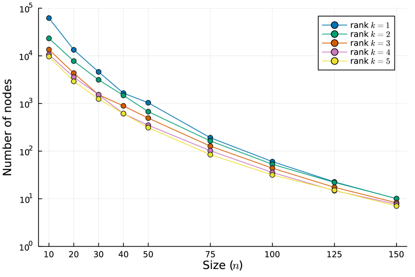
(a) Number of nodes explored

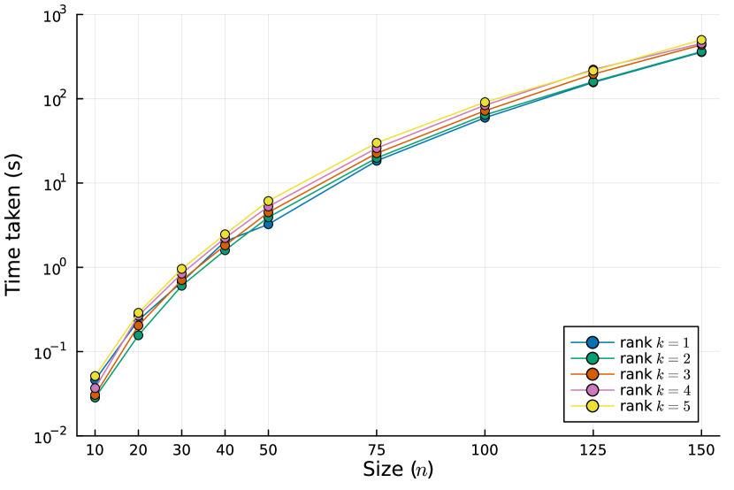
(b) Time taken at each node

Figure C.5: Comparison of nodes explored (a) and time spent per node (b) for rank-$k$ matrix completion with $2kn\log_{10}(n)$ filled entries, varying $n$ and $k$, with $\gamma=80.0$, averaged over 50 random instances per point.

Figure C.6 shows the relative optimality gap, at the root node and after branching, of 2-piece and 4-piece disjunctions applied to matrix completion problems of moderate to large sizes, with either $pkn$ or $pkn\log_{10}(n)$ filled entries ($p\in\{2.0,2.5,3.0\}$). From Figure C.6 we see that as $n$ increases, the root node relative gap reduces, but the improvement in relative gap after branching also diminishes. We can also compare 2-piece and 4-piece disjunctions: 4-piece disjunctions perform better for smaller-sized problems, whereas 2-piece disjunctions yield a better relative gap after branching for larger-sized problems (this is the same trend illustrated in Figure C.4). In the regime with $pkn\log_{10}(n)$ filled entries, the constant $p$ has a smaller impact on relative optimality gaps compared to that for $pkn$ filled entries.

(a) $pkn$ filled entries, 2-piece disjunctions

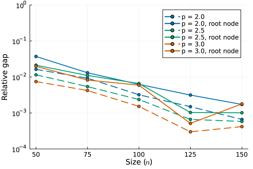
(b) $pkn\log_{10}(n)$ filled entries, 2-piece disjunctions

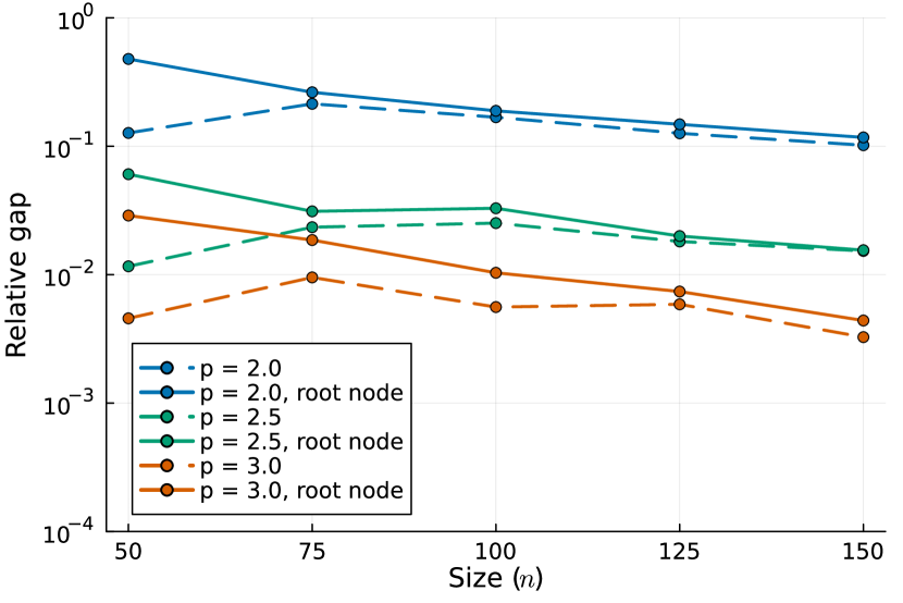
(c) $pkn$ filled entries, 4-piece disjunctions

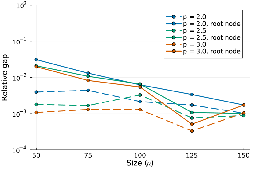
(d) $pkn\log_{10}(n)$ filled entries, 4-piece disjunctions

Figure C.6: Comparison of relative gap at the root node (dashed lines), and after branch-and-bound with a 3600s time limit (solid lines), against $n$ for rank-one matrix completion problems ($\gamma=80.0$) using two-piece or four-piece disjunctions (averaged over 20 random instances).

Tables C.10–C.13 also demonstrate this but also show that as $n$ increases, each individual SDP takes a longer time and so a smaller number of nodes are explored. This supports the hypothesis that as $n$ increases, in an appropriate sparsity regime, the root node relaxation is tight and alternating minimization recovers the globally optimal solution. Indeed, in Tables C.12–C.13 we can solve $200\times 200$ and $250\times 250$ matrix completion problems by performing alternating minimization (in negligible time) to get a good solution, and certifying its optimality in an hour by solving the root node relaxation. Figure C.7 illustrates the same trends but visualizes the variance over individual random instances by showing the empirical CDFs.

$n$	$p$	Nodes explored	Relaxation	Total time (s)	Relative gap	Relative gap
			solve time (s)		(root node)
50	2.0	$1035.35$	$3.227$	$>3600$	$4.96\text{\times}{10}^{-01}$	$9.12\text{\times}{10}^{-02}$
50	2.5	$1038.75$	$3.219$	$>3600$	$7.00\text{\times}{10}^{-02}$	$2.11\text{\times}{10}^{-02}$
50	3.0	$1053.75$	$3.174$	$>3600$	$3.21\text{\times}{10}^{-02}$	$1.56\text{\times}{10}^{-02}$
75	2.0	$191.55$	$18.3$	$>3600$	$2.63\text{\times}{10}^{-01}$	$1.59\text{\times}{10}^{-01}$
75	2.5	$199.3$	$17.54$	$>3600$	$3.11\text{\times}{10}^{-02}$	$1.98\text{\times}{10}^{-02}$
75	3.0	$197.15$	$17.77$	$>3600$	$1.91\text{\times}{10}^{-02}$	$1.26\text{\times}{10}^{-02}$
100	2.0	$59.5$	$59.95$	$>3600$	$1.93\text{\times}{10}^{-01}$	$1.31\text{\times}{10}^{-01}$
100	2.5	$59.85$	$59.72$	$>3600$	$3.29\text{\times}{10}^{-02}$	$2.48\text{\times}{10}^{-02}$
100	3.0	$59.35$	$60.36$	$>3600$	$1.03\text{\times}{10}^{-02}$	$7.95\text{\times}{10}^{-03}$
125	2.0	$23.85$	$152.6$	$>3600$	$1.48\text{\times}{10}^{-01}$	$1.26\text{\times}{10}^{-01}$
125	2.5	$24.4$	$148.7$	$>3600$	$2.00\text{\times}{10}^{-02}$	$1.82\text{\times}{10}^{-02}$
125	3.0	$24.2$	$150.2$	$>3600$	$7.39\text{\times}{10}^{-03}$	$5.77\text{\times}{10}^{-03}$
150	2.0	$11.0$	$340.2$	$>3600$	$1.14\text{\times}{10}^{-01}$	$1.01\text{\times}{10}^{-01}$
150	2.5	$11.35$	$334.3$	$>3600$	$1.55\text{\times}{10}^{-02}$	$1.35\text{\times}{10}^{-02}$
150	3.0	$11.1$	$337.5$	$>3600$	$4.39\text{\times}{10}^{-03}$	$2.75\text{\times}{10}^{-03}$

Table C.10: Results for rank-one matrix completion with 2-piece disjunctions starting with $pkn$ filled entries over different problem instances (average of 20 instances per row).

$n$	$p$	Nodes	Relaxation	Runtime (s)	Relative gap	Relative gap
			solve time (s)		(root node)
50	2.0	$654.6$	$5.235$	$>3600$	$4.78\text{\times}{10}^{-01}$	$1.27\text{\times}{10}^{-01}$
50	2.5	$580.32$	$5.588$	$3204.8$	$6.06\text{\times}{10}^{-02}$	$1.16\text{\times}{10}^{-02}$
50	3.0	$453.95$	$5.871$	$2183.8$	$2.89\text{\times}{10}^{-02}$	$4.57\text{\times}{10}^{-03}$
75	2.0	$137.25$	$25.89$	$>3600$	$2.63\text{\times}{10}^{-01}$	$2.14\text{\times}{10}^{-01}$
75	2.5	$133.1$	$26.71$	$>3600$	$3.11\text{\times}{10}^{-02}$	$2.34\text{\times}{10}^{-02}$
75	3.0	$123.79$	$29.09$	$>3600$	$1.86\text{\times}{10}^{-02}$	$9.52\text{\times}{10}^{-03}$
100	2.0	$47.0$	$76.66$	$>3600$	$1.89\text{\times}{10}^{-01}$	$1.68\text{\times}{10}^{-01}$
100	2.5	$44.6$	$80.94$	$>3600$	$3.29\text{\times}{10}^{-02}$	$2.52\text{\times}{10}^{-02}$
100	3.0	$34.05$	$84.9$	$2482.4$	$1.03\text{\times}{10}^{-02}$	$5.59\text{\times}{10}^{-03}$
125	2.0	$18.55$	$203.5$	$>3600$	$1.48\text{\times}{10}^{-01}$	$1.26\text{\times}{10}^{-01}$
125	2.5	$18.6$	$196.9$	$>3600$	$2.00\text{\times}{10}^{-02}$	$1.81\text{\times}{10}^{-02}$
125	3.0	$16.0$	$205.8$	$3082.3$	$7.39\text{\times}{10}^{-03}$	$5.88\text{\times}{10}^{-03}$
150	2.0	$8.3$	$456.7$	$>3600$	$1.17\text{\times}{10}^{-01}$	$1.02\text{\times}{10}^{-01}$
150	2.5	$8.1$	$479.2$	$>3600$	$1.55\text{\times}{10}^{-02}$	$1.53\text{\times}{10}^{-02}$
150	3.0	$7.95$	$460.5$	$>3600$	$4.39\text{\times}{10}^{-03}$	$3.26\text{\times}{10}^{-03}$

Table C.11: Results for rank-one matrix completion with 4-piece disjunctions starting with $pkn$ filled entries over different instances (avg. 20 instances per row).

$n$	$p$	Nodes	Relaxation	Runtime (s)	Relative gap	Relative gap
			solve time (s)		(root node)
50	2.0	$1051.2$	$3.175$	$>3600$	$3.72\text{\times}{10}^{-02}$	$1.63\text{\times}{10}^{-02}$
50	2.5	$1032.65$	$3.262$	$>3600$	$2.13\text{\times}{10}^{-02}$	$1.15\text{\times}{10}^{-02}$
50	3.0	$1018.8$	$3.332$	$>3600$	$1.98\text{\times}{10}^{-02}$	$7.46\text{\times}{10}^{-03}$
75	2.0	$191.3$	$18.35$	$>3600$	$1.31\text{\times}{10}^{-02}$	$9.24\text{\times}{10}^{-03}$
75	2.5	$191.2$	$18.38$	$>3600$	$1.10\text{\times}{10}^{-02}$	$5.41\text{\times}{10}^{-03}$
75	3.0	$187.9$	$18.79$	$>3600$	$8.23\text{\times}{10}^{-03}$	$4.21\text{\times}{10}^{-03}$
100	2.0	$60.65$	$59.09$	$>3600$	$6.24\text{\times}{10}^{-03}$	$3.21\text{\times}{10}^{-03}$
100	2.5	$58.4$	$61.4$	$>3600$	$6.56\text{\times}{10}^{-03}$	$2.36\text{\times}{10}^{-03}$
100	3.0	$58.1$	$61.8$	$>3600$	$5.91\text{\times}{10}^{-03}$	$1.52\text{\times}{10}^{-03}$
125	2.0	$21.7$	$154.1$	$2935.0$	$3.14\text{\times}{10}^{-03}$	$1.49\text{\times}{10}^{-03}$
125	2.5	$21.7$	$151.7$	$2669.8$	$1.03\text{\times}{10}^{-03}$	$6.62\text{\times}{10}^{-04}$
125	3.0	$20.1$	$155.3$	$2284.7$	$5.13\text{\times}{10}^{-04}$	$3.00\text{\times}{10}^{-04}$
150	2.0	$10.95$	$335.2$	$>3600$	$1.73\text{\times}{10}^{-03}$	$6.62\text{\times}{10}^{-04}$
150	2.5	$10.8$	$337.8$	$>3600$	$1.01\text{\times}{10}^{-03}$	$5.82\text{\times}{10}^{-04}$
150	3.0	$10.3$	$339.3$	$3404.0$	$1.79\text{\times}{10}^{-03}$	$4.18\text{\times}{10}^{-04}$
200	2.0	$1.45$	$1200.0$	$1563.0$	$6.06\text{\times}{10}^{-07}$	$9.65\text{\times}{10}^{-08}$
200	2.5	$1.4$	$1190.0$	$1496.6$	$5.04\text{\times}{10}^{-07}$	$1.96\text{\times}{10}^{-07}$
200	3.0	$1.4$	$1139.0$	$1462.1$	$4.69\text{\times}{10}^{-07}$	$5.25\text{\times}{10}^{-08}$
250	2.0	$1.2$	$3118.0$	$3581.6$	$5.54\text{\times}{10}^{-07}$	$9.22\text{\times}{10}^{-08}$
250	2.5	$1.19$	$3169.0$	$>3600$	$7.42\text{\times}{10}^{-07}$	$2.14\text{\times}{10}^{-07}$
250	3.0	$1.25$	$3175.0$	$>3600$	$5.96\text{\times}{10}^{-07}$	$1.44\text{\times}{10}^{-07}$

Table C.12: Results for rank-one matrix completion with 2-piece disjunctions starting with $pkn\log(n)$ filled entries over different instances (avg. 20 instances per row).

$n$	$p$	Nodes	Relaxation	Runtime (s)	Relative gap	Relative gap
			solve time (s)		(root node)
50	2.0	$439.4$	$5.5$	$1733.1$	$3.12\text{\times}{10}^{-02}$	$3.95\text{\times}{10}^{-03}$
50	2.5	$374.6$	$6.0$	$1483.6$	$2.10\text{\times}{10}^{-02}$	$1.79\text{\times}{10}^{-03}$
50	3.0	$248.4$	$5.2$	$429.4$	$1.98\text{\times}{10}^{-02}$	$1.08\text{\times}{10}^{-03}$
75	2.0	$86.9$	$28.6$	$1674.1$	$1.31\text{\times}{10}^{-02}$	$4.40\text{\times}{10}^{-03}$
75	2.5	$86.4$	$29.6$	$1862.2$	$1.07\text{\times}{10}^{-02}$	$1.67\text{\times}{10}^{-03}$
75	3.0	$74.3$	$28.1$	$1263.0$	$8.23\text{\times}{10}^{-03}$	$1.30\text{\times}{10}^{-03}$
100	2.0	$33.05$	$85.7$	$2350.6$	$6.24\text{\times}{10}^{-03}$	$2.15\text{\times}{10}^{-03}$
100	2.5	$30.7$	$88.6$	$2098.9$	$6.56\text{\times}{10}^{-03}$	$3.28\text{\times}{10}^{-03}$
100	3.0	$28.39$	$88.1$	$1858.3$	$5.44\text{\times}{10}^{-03}$	$1.29\text{\times}{10}^{-03}$
125	2.0	$13.84$	$212.4$	$2475.3$	$3.38\text{\times}{10}^{-03}$	$1.72\text{\times}{10}^{-03}$
125	2.5	$11.21$	$204.0$	$1725.8$	$1.08\text{\times}{10}^{-03}$	$7.61\text{\times}{10}^{-04}$
125	3.0	$10.65$	$205.1$	$1528.5$	$5.13\text{\times}{10}^{-04}$	$3.33\text{\times}{10}^{-04}$
150	2.0	$6.9$	$467.6$	$3135.6$	$1.73\text{\times}{10}^{-03}$	$1.03\text{\times}{10}^{-03}$
150	2.5	$7.15$	$456.1$	$3174.3$	$1.01\text{\times}{10}^{-03}$	$8.86\text{\times}{10}^{-04}$
150	3.0	$6.84$	$463.7$	$3092.4$	$1.73\text{\times}{10}^{-03}$	$1.05\text{\times}{10}^{-03}$
200	2.0	$1.4$	$1180.0$	$1506.3$	$6.06\text{\times}{10}^{-07}$	$6.07\text{\times}{10}^{-08}$
200	2.5	$1.5$	$1159.0$	$1506.9$	$5.04\text{\times}{10}^{-07}$	$1.08\text{\times}{10}^{-07}$
200	3.0	$1.55$	$1137.0$	$1533.1$	$4.69\text{\times}{10}^{-07}$	$8.96\text{\times}{10}^{-08}$
250	2.0	$1.27$	$3157.0$	$>3600$	$1.53\text{\times}{10}^{-06}$	$7.21\text{\times}{10}^{-07}$
250	2.5	$1.12$	$3112.0$	$3376.6$	$4.65\text{\times}{10}^{-07}$	$1.24\text{\times}{10}^{-07}$
250	3.0	$1.23$	$3077.0$	$>3600$	$8.79\text{\times}{10}^{-07}$	$9.32\text{\times}{10}^{-08}$

Table C.13: Results for rank-one matrix completion with four-piece disjunctions starting with $pkn\log(n)$ filled entries over different instances (avg. 20 instances per row).

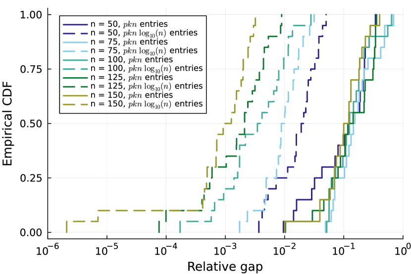
(a) $p=2.0$, 2-piece disjunctions

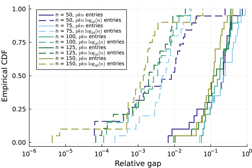
(b) $p=2.0$, 4-piece disjunctions

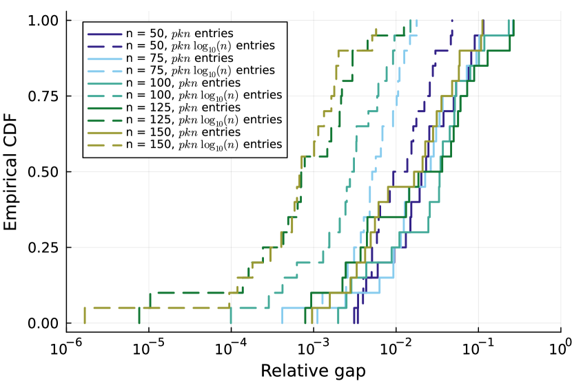
(c) $p=2.5$, 2-piece disjunctions

(d) $p=2.5$, 4-piece disjunctions

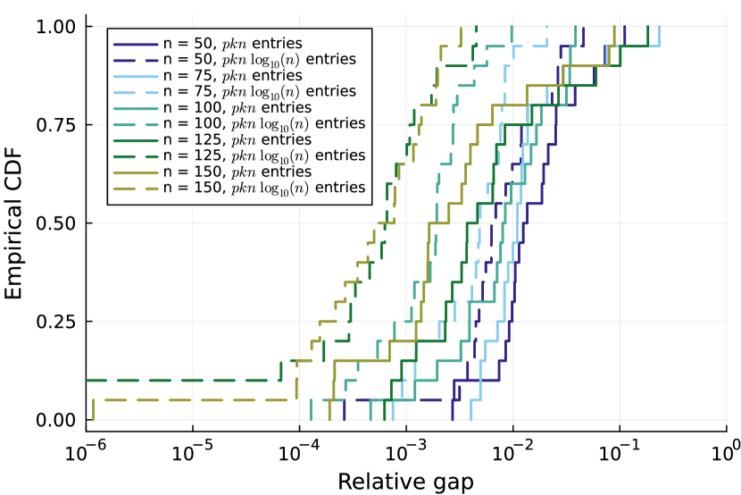
(e) $p=3.0$, 2-piece disjunctions

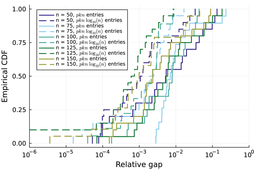
(f) $p=3.0$, 4-piece disjunctions

Figure C.7: Empirical CDF of relative gaps after branch-and-bound for 1 hour, for rank-one matrix completion problems (with $\gamma=80.0$) (across 20 random instances).

Figure 8(c) shows the absolute improvement in mean-squared error (MSE) after branching for 1 hour, as compared to the alternating minimization solution found at the root node, across different sparsity settings ($|\mathcal{I}|\propto n$, $|\mathcal{I}|\propto n\log_{10}(n)$, and $|\mathcal{I}|\propto n^{6/5}\log_{10}(n)$). These plots illustrate the MSE improvement (in absolute terms) which is more pronounced in the sparser regime, and for low values of rank $k$ other than $k=1$.

In a similar vein, Figure C.9 also shows the absolute improvement in MSE when comparing our approach to MFSGD (described in Jin et al. (2016), and found to be the best-performing benchmark of four methods studied in Bertsimas and Li (2020)). Across all parameter settings, our method yields a significant MSE improvement, with the improvement particularly stark in the sparser regime ($|\mathcal{I}|\propto n$). For more populous regimes, our approach yields a smaller improvement with larger ranks – this could be due to the time limit of 1 hour resulting in our methods not exploring many nodes and not improving over the alternating minimization solution found at the root node. Overall, these plots show the benefits of our optimality-focused approach.

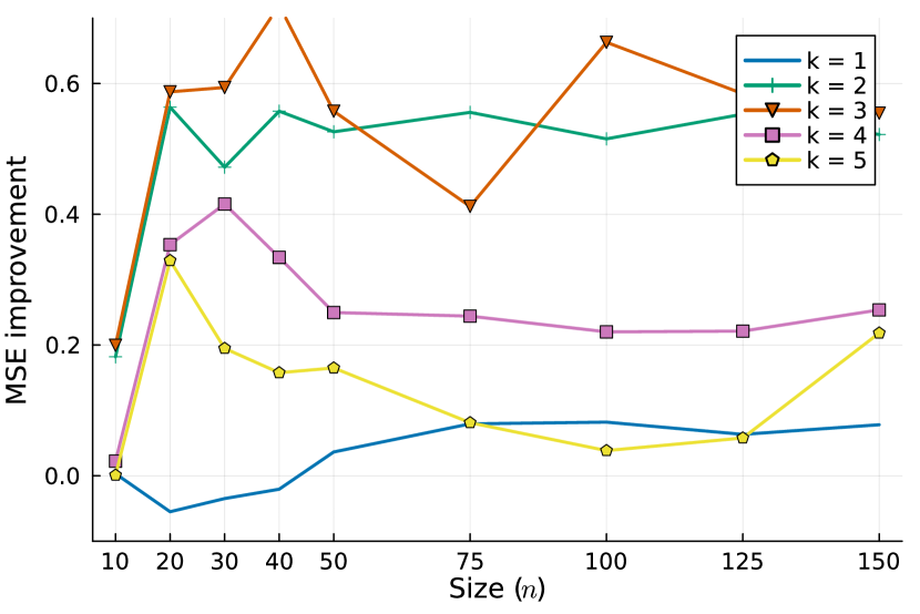
(a) $2kn$ filled entries

(b) $3kn$ filled entries

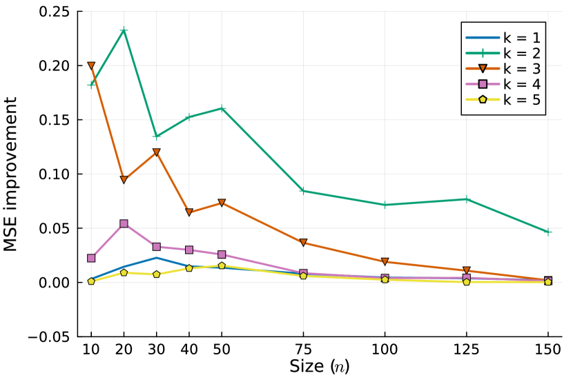
(c) $2kn\log_{10}(n)$ filled entries

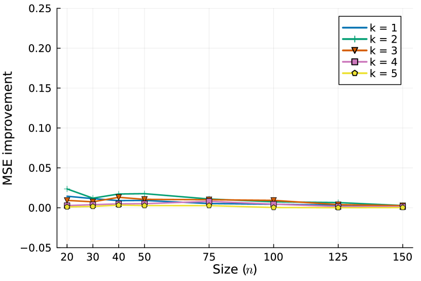
(d) $3kn\log_{10}(n)$ filled entries

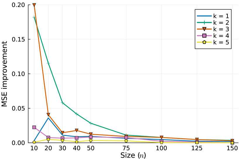
(e) $\left(2/10^{6/5}\right)kn^{6/5}\log_{10}(n)$ filled entries

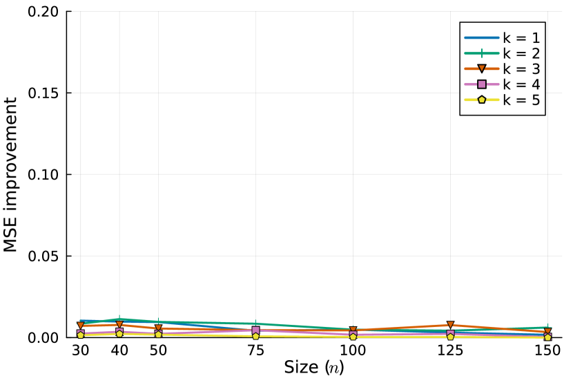
(f) $\left(3/10^{6/5}\right)kn^{6/5}\log_{10}(n)$ filled entries

Figure C.8: MSE improvement (in absolute terms) for rank-$k$ matrix completion problems against MFSGD, varying $n$ and $k$, with $\gamma=80.0$, averaged over 50 random instances per point.

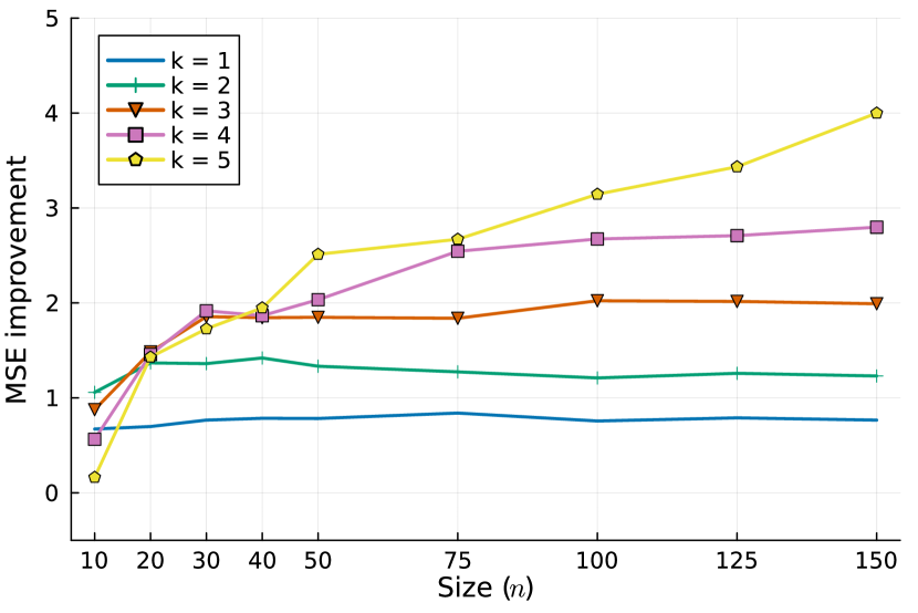
(a) $2kn$ filled entries

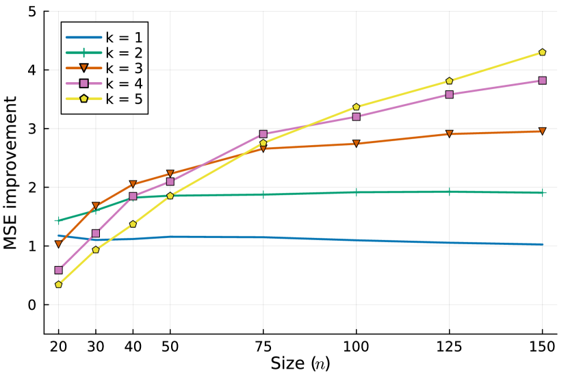
(b) $3kn$ filled entries

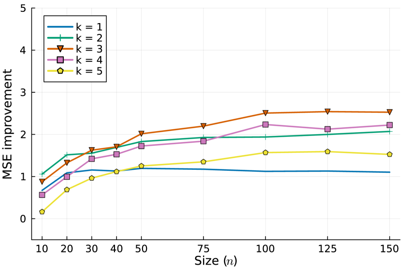
(c) $2kn\log_{10}(n)$ filled entries

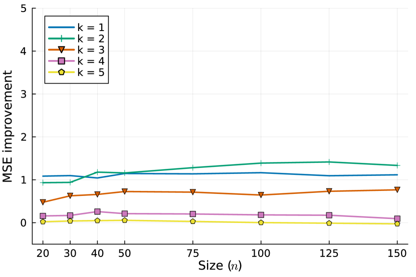
(d) $3kn\log_{10}(n)$ filled entries

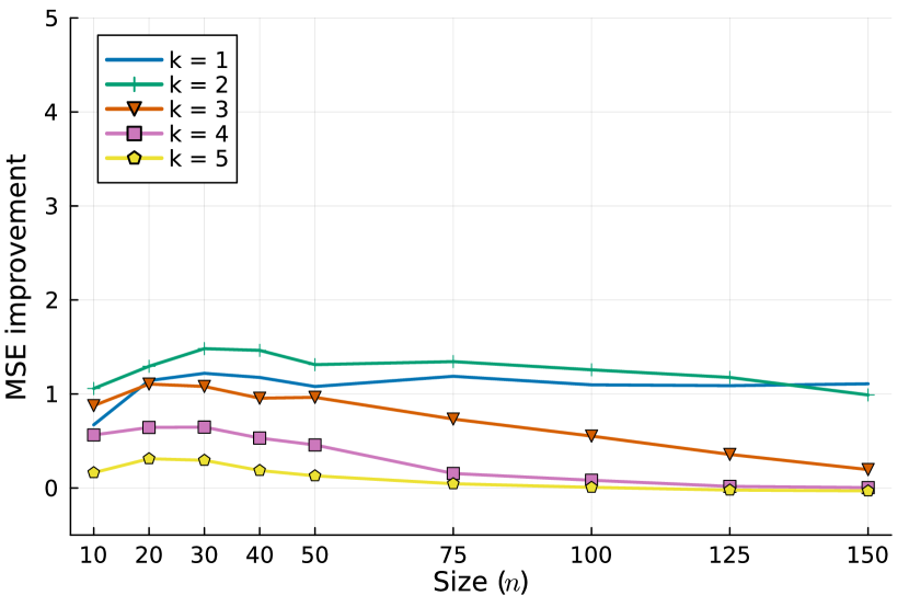
(e) $\left(2/10^{6/5}\right)kn^{6/5}\log_{10}(n)$ filled entries

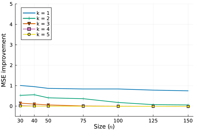
(f) $\left(3/10^{6/5}\right)kn^{6/5}\log_{10}(n)$ filled entries

Figure C.9: MSE improvement (in absolute terms) for rank-$k$ matrix completion problems against alternating minimization at the root node, varying $n$ and $k$, with $\gamma=80.0$, averaged over 50 random instances per point.