Revisiting the Architectures like Pointer Networks to Efficiently Improve the Next Word Distribution, Summarization Factuality, and Beyond

Abstract

Is the output softmax layer, which is adopted by most language models (LMs), always the best way to compute the next word probability? Given so many attention layers in a modern transformer-based LM, are the pointer networks redundant nowadays? In this study, we discover that the answers to both questions are no. This is because the softmax bottleneck sometimes prevents the LMs from predicting the desired distribution and the pointer networks can be used to break the bottleneck efficiently. Based on the finding, we propose several softmax alternatives by simplifying the pointer networks and accelerating the word-by-word rerankers. In GPT-2, our proposals are significantly better and more efficient than mixture of softmax, a state-of-the-art softmax alternative. In summarization experiments, without significantly decreasing its training/testing speed, our best method based on T5-Small improves factCC score by 2 points in CNN/DM and XSUM dataset, and improves MAUVE scores by 30% in BookSum paragraph-level dataset.

1 Introduction

When recurrent neural networks such as LSTM Hochreiter and Schmidhuber (1997) are the mainstream language model (LM) architecture, pointer networks, or so-called copy mechanisms (Gu et al., 2016), have been shown to improve the state-of-the-art LMs for next word prediction Merity et al. (2017) and summarizations (See et al., 2017) by a large margin. However, after transformer (Vaswani et al., 2017) becomes the dominating LM architectures, the pointer networks are rarely used in the state-of-the-art pretrained LMs.One major reason is that the attention mechanism in every transformer layer can learn to copy the words from the context, so it seems to be redundant to add a copying mechanism on top of the transformer.

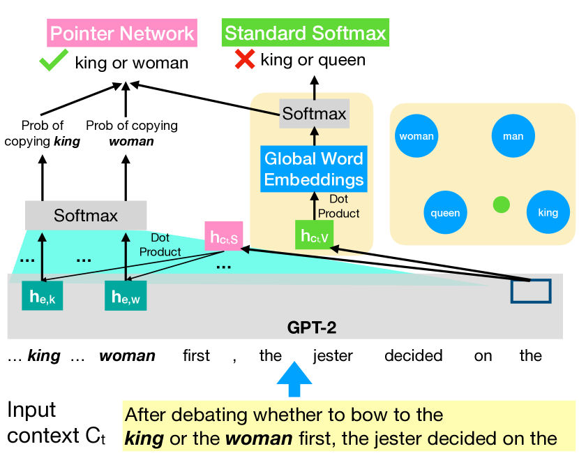
Figure 1: Illustration of the softmax bottleneck and pointer network using an example from Chang and McCallum (2022). GPT-2 cannot output both king or woman as the possible next word due to the parallelogram structure in the output word embedding space, while the pointer network could solve this by directly copying words from the context. The standard softmax estimate the probabilities of outputting king and woman by the dot products between the hidden state $\mathbf{h}_{c_{t},V}$ and their global word embeddings. By contrast, The pointer networks compute the dot products between the projected current hidden state $\mathbf{h}_{c_{t},S}$ and projected hidden states $\mathbf{h}_{e,.}$ for king and woman to estimate their probabilities.

In this paper, we demonstrate that the architectures like pointer networks can still substantially improve the state-of-the-art transformer LM architectures such as GPT-2 (Radford et al., 2019) and T5 (Raffel et al., 2020) mainly due to breaking the bottleneck of their final softmax layer (Yang et al., 2018; Chang and McCallum, 2022).

In Figure 1, we illustrate a simple example from Chang and McCallum (2022) to explain the softmax bottleneck and why the pointer networks could alleviate the problem. When predicting the next word, most LMs would try to output a hidden state $\mathbf{h}_{c_{t},V}$ that is close to all the next word possibilities. For example, when the next word should be either king or woman with similar probabilities, the ideal hidden state is supposed to be the average of the global output word embeddings of king and woman. However, there might be other interfering words (queen and man in this case) between the ideal next word candidates, which force the LM to output the wrong distribution.

To solve this problem, we can let the LMs predict the probability of copying the words in the context separately by paying attention to the previous hidden states Gu et al. (2016) and we call this kind of architecture pointer networks in this paper. That is, we can compute the dot products with the hidden states of king $\mathbf{h}_{e,k}$ and the hidden states of woman $\mathbf{h}_{e,w}$ rather than with their global output word embeddings in order to estimate the probabilities of copying these two words in the context. Our experiments show that the pointer networks consistently improve the performance of GPT-2 in next word prediction and the quality of summarization from T5 and BART.

Contrary to the mainstream explanation in previous pointer network literature, we discover that most of the improvements in our experiments do not come from the attention mechanism. To study these improvements, we propose a very simple pointer network variant that does not use any previous hidden states and we show that the proposed method can achieve similar improvements.

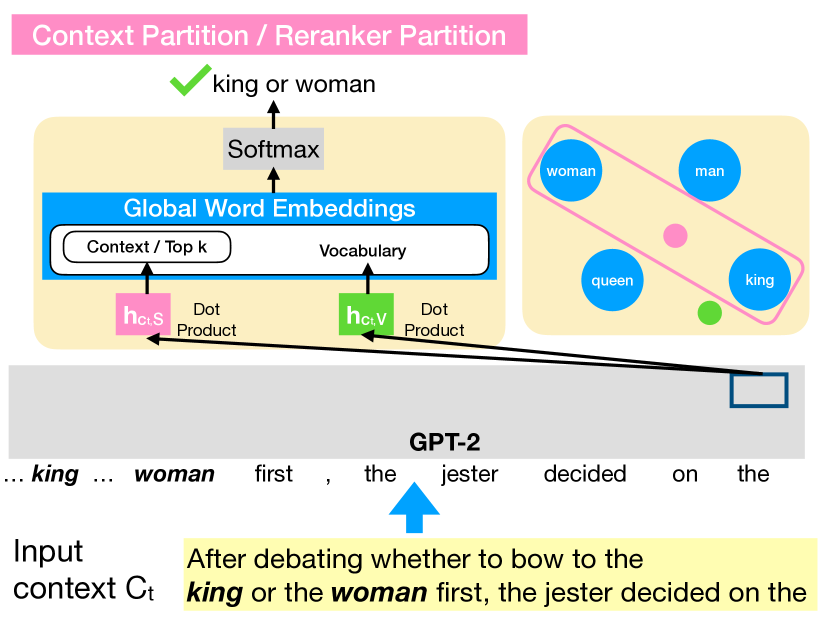
Figure 2: We simplify the pointer network / reranker by using another embedding $\mathbf{h}_{c_{t},S}$ for the words in the context / the top-k likely words.

As shown in Figure 2, we simply project the last hidden state into two embeddings. One embedding $\mathbf{h}_{c_{t},S}$ is to compute the dot product with the context words, and $\mathbf{h}_{c_{t},V}$ is for the dot product of the other words. Then, the GPT-2 can output the hidden state for context words $\mathbf{h}_{c_{t},S}$ as the average embedding of the king and woman without interfered by the words of man and queen that are handled by $\mathbf{h}_{c_{t},V}$. We call this method context partition. In addition to words in the context, we can also use another embedding for the top-k likely next words. This can be viewed as a very simple and efficient alternative to a reranker, so we call it reranker partition.

In our experiments, we show that the context partition performs similarly to pointer networks while combining a pointer network, context partition, and reranker partition would significantly outperform each individual method. Compared to the state-of-the-art solutions for alleviating the softmax bottleneck such as mixture of softmax (Yang et al., 2018; Chang and McCallum, 2022), our proposed method is more efficient while achieving lower perplexity on GPT-2. Furthermore, we find that adding a very expensive word-by-word reranker only improves our method slightly, which suggested the difficulty of further improving the final softmax layer over the proposed alternatives.

In the text completion task using GPT-2, we find that the proposed softmax alternatives reduce hallucination by copying more proper nouns from the context even though we did not provide any part-of-speech information during training. In summarization, our methods and pointer networks output a more specific summary, increase the factuality, and consistently improve 9 metrics, especially in the smaller language models. Finally, we show that the softmax bottleneck problem is not completely solved in GPT-3.5 in the limitation section.

1.1 Main Contributions

• We propose a series of efficient softmax alternatives that unify the ideas of pointer network, reranker, multiple embeddings, and vocabulary partitioning.

• We evaluate the proposed softmax alternatives in text completion tasks and summarization tasks using various metrics to identify where our methods improve the most.

• Our experiments indicate pointer networks and our proposed alternatives can still improve the modern transformer-based LMs. By breaking the softmax bottleneck, our methods learn to sometimes copy the context words to reduce generation hallucination and sometimes exclude the context words to reduce the repetition. Besides, we find that the softmax bottleneck problem won’t be completely solved by the huge size of GPT-3.5.

2 Background

Before introducing our method, we would first briefly review the problem we are solving and its state-of-the-art solutions.

2.1 Softmax Bottleneck Problem

Most LMs use a softmax layer to compute the final probability of predicting the word $x$:

$$P_{M}(x|c_{t})=\frac{\text{exp}(\text{Logit}(x,c_{t}))}{\sum_{x^{\prime}}\text{exp}(\text{Logit}(x^{\prime},c_{t}))},$$ (1)

where $c_{t}$ is the context words. Typically, the logit $\text{Logit}(x,c_{t})=({\bm{h}}^{M}_{c_{t}})^{T}{\bm{w}}_{x}$, ${\bm{h}}^{M}_{c_{t}}$ is the $M$th-layer hidden state given the input context $c_{t}$ and ${\bm{w}}_{x}$ is the output word embeddings for $x$.

One problem is that the output word embeddings ${\bm{w}}_{x}$ are global and independent to the context. After pretraining, the similar words would have similar output word embeddings. However, the similarity structure in the word embedding space might prevent LMs from outputting the desired distribution. The parallelogram structure among the embeddings of king, queen, woman, and man is a simple example. Chang and McCallum (2022) generalize this observation and show that some words in a small subspace would create some multi-mode distributions that a LM cannot output using a single hidden state ${\bm{h}}_{c_{t}}$ in the softmax layer.

2.2 Mixture of Softmax Method

To overcome the bottleneck, one natural solution is to have multiple hidden states and each hidden state corresponds to a group of possible words (Yang et al., 2018). For example, we can have one hidden state for king and another hidden state for woman.

One major concern of this mixture of softmax (MoS) approach is the computational overhead. MoS needs to compute the final softmax multiple times and merge their resulting distributions. That is, we need to compute the dot products between every hidden state and all the words in the vocabulary, which is expensive especially when the vocabulary size is large.

2.3 Multiple Input State Enhancement

In MoS, the multiple hidden states come from the linear projections of the last hidden state. Chang and McCallum (2022) point out that the total degree of freedom among the multiple hidden states is limited by the dimensionality of the hidden state.

To allow LMs to move multiple hidden states more freely, Chang and McCallum (2022) propose to concatenate the projection of a block of hidden state with the last hidden state ${\bm{h}}_{c_{t}}^{M}$ so as to increase its dimensionality:

$${\bm{q}}_{c_{t}}={\bm{h}}_{c_{t}}^{M}\oplus GELU\left(L^{h}(\oplus_{i,m}{\bm{h}}_{c_{t-i}}^{M-m})\right),$$ (2)

where $GELU$ is the non-linear transformation used in GPT-2 and $L^{h}$ is a linear transformation that allows us to consider more hidden states without significantly increasing the model size. $\oplus_{i,m}{\bm{h}}_{c_{t-i}}^{M-m}$ is the concatenation of a block of hidden states. We set the block size to be 3x3 in our GPT-2 experiments and 1x3 in our summarization experiments (i.e., considering the last 3 hidden states in the last layer as shown in Figure 3).

	Abbr.	Partition ($S$)	Word Emb (${\bm{e}}_{x}$)
Context Partition	C	Decoder context	Global word emb
Encoder Partition	E	Encoder input	Global word emb
PS (LD) (Merity et al., 2017)	P	Decoder context	Decoder state
PG (LE) (See et al., 2017)		Encoder input	Encoder state
Reranker Partition	R	Top k	Global word emb

Table 1: Comparison of different softmax alternatives and their abbreviation (Abbr.) using Equation 3. PS: Pointer Sentinel. PG: Pointer Generator. LD: local decoder embedding. LE: local encoder embedding.

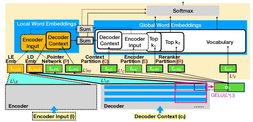
Figure 3: Architectures of our method for T5/BART that computes $\text{Logit}_{CEPR}$ in Equation 6. In GPT-2, we use same architecture except that we take the 3x3 input hidden state block rather than the 1x3 block and there are no encoder-related components, which are marked by dotted lines.

3 Methods

To break the softmax bottleneck more efficiently compared to MoS, our overall strategy is simple. If we can identify a small partition of words that are very likely to become the next word, we can just compute the dot products between a hidden state and the embeddings of these likely words instead of all the words as in MoS. For example, if we can identify king and woman are much more likely to appear than queen and man, we can only compute the dot product between a hidden state and the embeddings of king and woman without being interfered by other words.

Specifically, when we compute the next word probability in Equation 1, the logit of the word $x$ given the context $c_{t}$

$$\text{Logit}(x,c_{t})=\left\{\begin{matrix}[l]{\bm{f}}_{c_{t},S}^{T}{\bm{e}}_{x}\;\;\;\text{if}\;x\in S\\ {\bm{f}}_{c_{t},V}^{T}{\bm{w}}_{x}\;\;\text{O/W}\end{matrix}\right.,$$ (3)

where ${\bm{f}}_{c_{t},S}=L_{S}^{f}({\bm{q}}_{c_{t}})$ and ${\bm{f}}_{c_{t},V}=L_{V}^{f}({\bm{q}}_{c_{t}})$ are the linear projections of the hidden state concatenation ${\bm{q}}_{c_{t}}$ in Equation 2. As shown in Table 1, different softmax alternatives have different ways of constructing this set $S$ and use different word embeddings ${\bm{e}}_{x}$.

To simplify our explanation, we will focus on the decoder-only LM (i.e., GPT-2) first and extend our method to encoder-decoder LM (i.e., T5 and BART).

3.1 GPT-2

We will explain each softmax alternative individually and their connections to previous work such as pointer networks or rerankers.

3.1.1 Pointer Network (P) as Local Word Embedding

Similar to Pointer Sentinel (PS) (Merity et al., 2017), we treat the words in the context differently ($S=\{x|x\in c_{t}\}$) and let their word embeddings ${\bm{e}}_{x}$ come from the previous hidden states:

$${\bm{e}}_{x}={\bm{f}}_{x,c_{t},LD}=\frac{\sum_{i=1}^{t}\mathbbm{1}_{{c_{t}^{i}}=x}L_{LD}^{f}({\bm{q}}_{c_{t}^{i}})}{\sum_{i=1}^{t}\mathbbm{1}_{{c_{t}^{i}}=x}},$$ (4)

where $c_{t}^{i}$ is the $i$th input words in the context $c_{t}$, $L_{LD}^{f}$ is a linear layer, and $\mathbbm{1}_{{c_{t}^{i}}=x}=1\;\;\text{if}\;c_{t}^{i}=x$.

As a result, we can use the GPT-2 model to not only predict the hidden state ${\bm{f}}_{c_{t},S}={\bm{f}}_{c_{t},PD}=L_{PD}^{f}({\bm{q}}_{c_{t}})$ and ${\bm{f}}_{c_{t},V}$ but also predict the word embedding of context words ${\bm{e}}_{x}$. Unlike the global word embedding ${\bm{w}}_{x}$, the local word embedding ${\bm{e}}_{x}$ is context-dependent, so the LM can break the softmax bottleneck by adjusting the similarity of words based on the context. For example, GPT-2 could increase the similarity between ${\bm{e}}_{\text{king}}$ and ${\bm{e}}_{\text{woman}}$ to output the high probability for both words easily.

We call this version of pointer network local decoder (LD) embedding, which has some minor differences compared to PS (Merity et al., 2017) and other variants. For example, we merge their logits while PS merges their probabilities. PS does not do normalization when computing ${\bm{e}}_{x}$. In our experiments, we would show that these pointer network variants all have very similar improvements in modern LMs.

3.1.2 Context Partition (C)

To understand the source of the improvements from pointer networks, we simplify their architectures by setting the word embedding ${\bm{e}}_{x}={\bm{w}}_{x}$ and the partition $S$ is still the set of context words. Although much simpler, the LM with this context partition method can still break the softmax bottleneck by properly coordinating the hidden state specifically for the context words ${\bm{f}}_{c_{t},S}={\bm{f}}_{c_{t},C}=L_{C}^{f}({\bm{q}}_{c_{t}})$ and the hidden state for other words ${\bm{f}}_{c_{t},V}$. Compared to the pointer network, one advantage of context partition is that the LM can still leverage the learned global word similarity when estimating the probabilities of context words.

3.1.3 Reranker Partition (R)

In some cases, the possible next words might not be mentioned in the context. For example, in the context My favorite actor is Ryan [MASK], the next word could be Reynolds, Gosling, or the last names of other Ryan. Hence, using only the context partition does not completely solve the multimodal distribution problem.

Inspired by the idea of the reranker, we set $S$ to be the top $k$ words with the highest logits ${\bm{f}}_{c_{t},V}^{T}{\bm{w}}_{x}$. In practice, finding an ideal $k$ could be difficult. When $k$ is small, the reranker partition might not include the very likely next word. When $k$ is large, the reranker partition might not be able to separate the output candidates and the interfering words. To alleviate the problem, we can have multiple reranker partitions and use different hidden state embeddings (e.g., ${\bm{f}}_{c_{t},R1}$ and ${\bm{f}}_{c_{t},R2}$) for different partitions.

3.1.4 Hybrid Approach (CPR)

Local embeddings in the pointer networks and global embeddings in the context partition are complementary. Using local embeddings is representational powerful while using global embedding can leverage the global similarity of words. Hence, we can combine the two methods by summing their dot products.

For the methods that use different $S$, we can simply determine an order of computing the dot products and let the later dot products overwrite the existing values. In our experiments, we always use the order illustrated in Figure 3. That is, we compute the logits ($\text{Logit}_{CPR}(x,c_{t})$) by

$$\left\{\begin{matrix}[l]{\bm{f}}_{c_{t},C}^{T}{\bm{w}}_{x}+{\bm{f}}_{c_{t},PD}^{T}{\bm{f}}_{x,c_{t},LD}\;\;\text{if}\;x\in c_{t}\\ {\bm{f}}_{c_{t},R1}^{T}{\bm{w}}_{x}\;\;\text{if}\;x\in W(k_{1})-c_{t}\\ {\bm{f}}_{c_{t},R2}^{T}{\bm{w}}_{x}\;\;\text{if}\;x\in W(k_{2})-W(k_{1})-c_{t}\\ {\bm{f}}_{c_{t},V}^{T}{\bm{w}}_{x}\;\;\text{O/W}\end{matrix}\right.,$$ (5)

where $W(k_{2})$ is the top $k_{2}$ words with the highest ${\bm{f}}_{c_{t},V}^{T}{\bm{w}}_{x}$ and $W(k_{1})$ is the top $k_{1}$ words with the highest $\max({\bm{f}}_{c_{t},V}^{T}{\bm{w}}_{x},{\bm{f}}_{c_{t},R2}^{T}{\bm{w}}_{x})$.

3.2 T5 and BART

In the encoder-decoder architectures, our local decoder embedding, context partition, and reranker partitions are still applicable. Besides, we can leverage the words in the encoder input to further improve the performance.

3.2.1 Encoder Partition (E) and Local Encoder Embedding (P)

Similar to the context partition, the encoder partition handles the words in the encoder input $I$ differently by setting $S=\{x|x\in I\}$ and using the global word embedding ${\bm{e}}_{x}={\bm{w}}_{x}$.

As in Equation 4, we can also let the hidden states in the last layer pass through another linear layer $L_{LE}^{f}()$ to predict the embeddings of the words in the encoder input. The method is called local encoder (LE) embedding.

3.2.2 Hybrid Approach (CEPR)

Similar to GPT-2, we combine local encoder embedding and encoder partition for computing the probabilities of the words that are in the encoder context but not in the decoder context. As shown in Figure 3, we compute $\text{Logit}_{CEPR}(x,c_{t})$ by

$$\left\{\begin{matrix}[l]{\bm{f}}_{c_{t},C}^{T}{\bm{w}}_{x}+{\bm{f}}_{c_{t},PD}^{T}{\bm{f}}_{x,c_{t},LD}\;\;\text{if}\;x\in c_{t}\\ {\bm{f}}_{c_{t},E}^{T}{\bm{w}}_{x}+{\bm{f}}_{c_{t},PE}^{T}{\bm{f}}_{x,I,LE}\;\;\;\text{if}\;x\in I-c_{t}\\ {\bm{f}}_{c_{t},R1}^{T}{\bm{w}}_{x}\;\;\text{if}\;x\in W(k_{1})-c_{t}-I\\ {\bm{f}}_{c_{t},V}^{T}{\bm{w}}_{x}\;\;\;\text{O/W}\end{matrix}\right.,$$ (6)

which is the same as Equation 5 except that we add the encoder partition and local encoder embedding, and we remove the second reranker partition.

4 Experiments

The pointer network was a popular technique in language modeling Merity et al. (2017) and summarization (See et al., 2017). Thus, we also focus on these two fundamental applications.

	GPT-2 Small				GPT-2 Medium
Model Name	Size	Time (ms)	OWT ($\downarrow$)	Wiki ($\downarrow$)	Size	Time (ms)	OWT ($\downarrow$)	Wiki ($\downarrow$)
Softmax (GPT-2)	125.0M	82.9	18.96	24.28	355.9M	207.8	15.81	20.12
Softmax + Mi	130.9M	85.6	18.74	24.08	366.4M	213.8	15.71	20.07
Mixture of Softmax (MoS) (Yang et al., 2018)	126.2M	130.2	18.97	24.10	358.0M	262.9	15.71	19.95
MoS + Mi (Chang and McCallum, 2022)	133.3M	133.2	18.68	23.82	370.6M	268.2	15.61	19.86
Pointer Generator (PG) (See et al., 2017)	126.2M	106.0	18.67	23.70	358.0M	237.8	15.72	19.95
Pointer Sentinel (PS) (Merity et al., 2017)	126.2M	94.1	18.70	23.79	358.0M	218.3	15.72	19.95
Softmax + R:20 + Mi	132.1M	90.4	18.67	24.03	368.5M	203.6	15.64	19.94
Softmax + R:20,100 + Mi	133.3M	101.1	18.69	23.93	370.6M	228.5	15.61	19.89
Softmax + C + Mi	132.1M	94.8	18.48	23.56	368.5M	222.7	15.60	19.83
Softmax + P + Mi	133.3M	99.1	18.58	23.66	370.6M	214.7	15.63	19.90
PG + Mi	133.3M	111.2	18.43	23.43	370.6M	242.5	15.60	19.89
PS + Mi	133.3M	98.0	18.48	23.53	370.6M	224.6	15.60	19.87
Softmax + CR:20,100 + Mi	134.5M	113.3	18.46	23.48	372.7M	234.5	15.54	19.75
Softmax + CPR:20,100 + Mi	136.8M	119.9	18.43	23.42	376.9M	249.9	15.53	19.71
MoS + CPR:20,100 + Mi	139.2M	165.1	18.39	23.29	381.1M	300.6	15.44	19.57

Table 2: Comparison of different methods on top of GPT-2. Wiki and OWT refer to the testing perplexity of Wikipedia 2021 and OpenWebText, respectively. Lower perplexity is better. Time is the inference time of a batch; Mi is the multiple input hidden state enhancement; C is the context partition; R:20,100 is the reranker partition with $k_{1}=20$ and $k_{2}=100$; P is the pointer network (i.e., local decoder embedding). Please see Equation 5 for the details of CPR. The best scores are highlighted.

4.1 GPT-2

We follow the setup in Chang and McCallum (2022) to continue training GPT-2 on Wikipedia 2021 and OpenWebText (Radford et al., 2019).

4.1.1 Perplexity Comparison

In Table 2, we first compare their predictions on the next word distribution using the testing data perplexity, which is a standard metric in the LM architecture studies. In the table, Mi refers to multiple input state enhancement, which is proposed to break the softmax bottleneck more effectively (please see details in Section 2.3 and Chang and McCallum (2022)).

As we can see, Softmax + CPR:20,100 + Mi, which combines all the efficient approaches (i.e., context partition, reranker partition, and local decoder embedding), results in better performance and faster inference speed than the mixture of softmax (MoS) (Yang et al., 2018; Chang and McCallum, 2022). The inference speed is measured by our pure PyTorch implementation, which we believe could be further accelerated by implementing some new PyTorch operations using CUDA code.

If only using one method, the context partition (Softmax + C + Mi) is better than the reranker partitions (Softmax + R:20,100 + Mi) while performing similarly compared to local decoder word embedding (Softmax + P + Mi), Pointer Generator (PG + Mi) (See et al., 2017), and Pointer Sentinel (PS + Mi) (Merity et al., 2017). Their similar performances indicate that the improvement of pointer networks come from breaking the softmax bottleneck. The significantly better performance of PS + Mi compared to PS further supports the finding.

To know how well our method breaks the softmax bottleneck, we implement a word-by-word reranker model on GPT-2, which appends the most likely 100 words to the context when predicting each next word (see Section C.3 for more details). In Table 3, we show that our efficient softmax alternative Softmax + CPR:20,100 + Mi achieves significantly lower perplexity. Furthermore, the word-by-word reranker is at least 10 times slower during training. Combining word-by-word reranker with our method only improves the perplexity very slightly, which suggests the challenges of further improving LM by breaking softmax bottleneck.

Softmax + Mi	29.33	Softmax + wbwR:100 + Mi	28.89
Softmax +	28.46	Softmax +	28.40
CPR:20,100 + Mi		CPR:20,100 + wbwR:100 + Mi

Table 3: Comparison between our method and word-by-word reranker for the most likely 100 words (wbwR:100). The numbers are the validation perplexities on Wikipedia 2021 after training for 0.15 epochs.

	All		Proper Noun
Model Name	Ref	Context	Ref	Context
Softmax + Mi	22.90	24.04	7.49	14.84
MoS + Mi	22.88	23.98	7.70	15.49
PS + Mi	22.85	25.01	8.16	18.21
Softmax + CPR:20,100 + Mi	23.05	25.36	8.16	17.92

Table 4: ROUGE-1 F1 (%) of different methods on GPT-2. We compare the scores between the generated text and the reference (i.e., continuation), and between the generation and context. More methods and metrics are reported in Table 8.

4.1.2 Generated Text Comparison

Next, we would like to understand how the distribution improvement affects the text generation. We sample some contexts in the test set of Wikipedia 2021 and compare the generated text quality of the different models given the contexts. The quality is measured by the ROUGE-1 F1 scores between the generated text and the actual continuation. To know how much the different models copy from the context, we also report the ROUGE-1 scores between the generation and the contexts.

The results in Table 4 show that different methods have very similar overall ROUGE-1 scores. Nevertheless, compared to Softmax + Mi, Softmax + CPR:20,100 + Mi is 21% more likely to copy the proper nouns (i.e., entity names) from the context and 9% more likely to generate the proper nouns in the actual continuation. This suggests that our method could alleviate the common incoherence problem of entities in generated text (Shuster et al., 2022; Papalampidi et al., 2022; Zhang et al., 2022; Guan et al., 2022; Goyal et al., 2022b). In Table 8, we compare methods using more metrics to further support the conclusion.

Input Context	There are plates, keys, scissors, toys, and balloons in front of me, and I pick up the	Choosing between John, Alex, Mary, Kathryn, and Jack, I decided to first talk to	I like tennis, baseball, golf, basketball, and
Softmax + Mi	keys 0.108, pieces 0.045, key 0.036, phone 0.020, balloons 0.019	John 0.108, the 0.102, them 0.095, him 0.045, my 0.032	tennis 0.089, baseball 0.075, football 0.041, basketball 0.036, I 0.032
Mixture of Softmax (MoS) + Mi	keys 0.085, phone 0.035, key 0.031, pieces 0.029, balloons 0.016	John 0.099, the 0.097, them 0.083, Alex 0.055, Mary 0.040	baseball 0.076, basketball 0.062, tennis 0.059, golf 0.037, bad 0.035
Pointer Sentinel (PS) + Mi	keys 0.091, plates 0.079, scissors 0.050, balloons 0.034, toys 0.033	John 0.130, the 0.105, Alex 0.076, them 0.076, Mary 0.037	tennis 0.095, golf 0.050, baseball 0.043, I 0.038, other 0.038
Softmax + CPR:20,100 + Mi	keys 0.077, balloons 0.052, plates 0.036, toys 0.030, pieces 0.030	the 0.106, John 0.099, my 0.060, Alex 0.057, them 0.044	football 0.075, volleyball 0.058, soccer 0.056, I 0.047, bad 0.038

Table 5: Prediction visualization of three input contexts. We show the top five words with the highest prediction probabilities of each model. The reasonable next word predictions are boldfaced.

	CNN/DM				XSUM				BookSum Paragraph				SAMSUM
Model Name	R1	CIDEr	factCC	MAUVE	R1	CIDEr	factCC	MAUVE	R1	CIDEr	factCC	MAUVE	R1	CIDEr	factCC	MAUVE
T5-Small
Softmax (S)	38.255	0.442	0.462	0.861	28.713	0.446	0.254	0.939	16.313	0.083	0.424	0.328	39.472	0.817	0.577	0.898
CopyNet (Gu et al., 2016)	37.990	0.438	0.482	0.865	28.573	0.442	0.274	0.940	16.666	0.092	0.439	0.402	39.525	0.853	0.579	0.924
PG (See et al., 2017)	37.913	0.442	0.467	0.874	28.777	0.450	0.257	0.931	16.432	0.088	0.429	0.376	32.451	0.585	0.552	0.153
PS (Merity et al., 2017)	38.058	0.444	0.466	0.854	28.442	0.435	0.267	0.932	16.408	0.090	0.436	0.395	38.731	0.817	0.578	0.865
S + R:20	37.881	0.433	0.474	0.872	28.557	0.440	0.256	0.931	16.336	0.086	0.431	0.370	39.073	0.752	0.579	0.847
S + E	38.137	0.441	0.477	0.866	28.723	0.444	0.272	0.942	16.542	0.090	0.435	0.390	39.056	0.784	0.579	0.904
S + CE	38.461	0.460	0.475	0.874	29.155	0.464	0.270	0.948	16.628	0.093	0.436	0.403	40.055	0.835	0.583	0.943
S + CER:20	38.346	0.450	0.482	0.890	29.067	0.459	0.276	0.942	16.638	0.093	0.436	0.400	40.505	0.846	0.580	0.915
S + CEPR:20	38.807	0.456	0.481	0.877	29.395	0.474	0.273	0.942	16.894	0.098	0.440	0.418	40.127	0.891	0.582	0.946
S + CEPR:20 + Mi	38.675	0.451	0.475	0.878	29.348	0.470	0.275	0.946	16.738	0.096	0.438	0.426	40.328	0.874	0.582	0.932
T5-Base
Softmax (S)	40.198	0.504	0.478	0.907	33.571	0.667	0.249	0.979	16.761	0.096	0.424	0.467	44.348	1.046	0.574	0.986
CopyNet (Gu et al., 2016)	39.940	0.507	0.484	0.903	33.557	0.666	0.253	0.979	16.918	0.101	0.430	0.531	44.141	1.052	0.570	0.973
PG (See et al., 2017)	39.982	0.489	0.485	0.911	33.605	0.663	0.255	0.982	16.611	0.095	0.423	0.463	37.597	0.784	0.548	0.140
PS (Merity et al., 2017)	40.018	0.495	0.483	0.914	33.638	0.672	0.249	0.983	16.905	0.100	0.428	0.504	43.098	1.008	0.575	0.946
S + CEPR:20	40.354	0.511	0.487	0.919	33.700	0.675	0.260	0.980	16.997	0.100	0.432	0.549	44.860	1.064	0.573	0.963
S + CEPR:20 + Mi	40.510	0.506	0.481	0.918	33.853	0.683	0.263	0.983	16.975	0.101	0.431	0.546	44.488	1.055	0.576	0.980
BART Base
Softmax (S)	39.390	0.428	0.479	0.900	35.675	0.814	0.241	0.985	16.393	0.094	0.414	0.404	45.132	1.129	0.567	0.966
CopyNet (Gu et al., 2016)	39.385	0.438	0.484	0.906	35.515	0.814	0.251	0.988	16.642	0.100	0.422	0.495	44.316	1.103	0.577	0.970
PG (See et al., 2017)	39.264	0.444	0.489	0.909	35.653	0.810	0.242	0.987	16.402	0.094	0.414	0.402	45.278	1.153	0.578	0.977
PS (Merity et al., 2017)	39.471	0.459	0.490	0.906	35.411	0.809	0.247	0.986	16.718	0.099	0.422	0.492	44.575	1.084	0.573	0.974
S + R:20	39.181	0.434	0.475	0.905	35.586	0.808	0.247	0.988	16.419	0.096	0.418	0.439	45.024	1.154	0.572	0.970
S + E	39.267	0.439	0.483	0.907	35.698	0.819	0.241	0.988	16.442	0.097	0.415	0.429	44.825	1.106	0.572	0.981
S + CE	39.416	0.442	0.481	0.908	35.727	0.812	0.241	0.988	16.555	0.096	0.417	0.435	44.295	1.116	0.572	0.985
S + CER:20	39.421	0.439	0.482	0.900	35.576	0.812	0.236	0.987	16.553	0.096	0.418	0.454	45.054	1.150	0.576	0.988
S + CEPR:20	39.723	0.441	0.483	0.908	35.732	0.822	0.242	0.986	16.664	0.098	0.420	0.467	44.732	1.115	0.575	0.974
S + CEPR:20 + Mi	39.626	0.442	0.482	0.907	35.846	0.828	0.245	0.986	16.597	0.097	0.419	0.466	44.728	1.132	0.574	0.988
BART Large
Softmax (S)	40.749	0.424	0.495	0.899	38.828	0.921	0.263	0.988	17.271	0.103	0.420	0.461	47.384	1.187	0.574	0.975
CopyNet (Gu et al., 2016)	40.622	0.407	0.487	0.890	38.576	0.920	0.258	0.989	17.342	0.106	0.425	0.512	47.911	1.232	0.573	0.980
PG (See et al., 2017)	40.766	0.407	0.489	0.902	38.869	0.944	0.256	0.990	17.289	0.103	0.424	0.470	47.737	1.199	0.573	0.964
PS (Merity et al., 2017)	40.643	0.424	0.502	0.907	38.886	0.952	0.255	0.988	17.382	0.105	0.426	0.527	48.253	1.246	0.574	0.986
S + CEPR:20	40.876	0.458	0.500	0.925	38.991	0.955	0.248	0.990	17.337	0.106	0.423	0.467	47.253	1.298	0.572	0.976
S + CEPR:20 + Mi	40.441	0.463	0.500	0.927	38.705	0.965	0.242	0.991	16.995	0.105	0.421	0.482	47.488	1.271	0.571	0.986

Table 6: The performance on test sets of four summarization datasets. R1 is ROUGE-1 F1 (%). E refers to the encoder partition; C is the context partition; R:20 is the reranker partition with $k_{1}=20$; The P in CEPR means using the pointer networks for both encoder (LE) and decoder (LD); Mi is the multiple input hidden state enhancement; PS means Pointer Sentinel and PG means Pointer Generator. CEPR is described in Equation 6. The model size, inference time, and more metrics are reported in Table 9 and Table 10.

4.1.3 Qualitative Analysis

In Table 5, we visualize some distributions to explain our improvements. The softmax layer of GPT-2 is unable to properly learn to copy or exclude the word from the input context. For example, Softmax + Mi and MoS + Mi might output “There are plates, keys, scissors, toys, and balloons in front of me, and I pick up the phone”, which causes a hallucination problem, while Softmax + CPR:20,100 + Mi and Pointer Sentinel (PS) + Mi can output the mentioned options with similar probability by copying the words in the context. In addition, GPT-2, MoS, and PS + Mi are very likely to output “I like tennis, baseball, golf, basketball, and tennis”. This repetition problem happens because the next word should be some words similar to the listed sports names except for the sports that have been mentioned and the softmax layer has difficulties in outputting a donut-shape next word distribution in embedding space. In contrast, Softmax + CPR:20,100 + Mi can learn to exclude the listed sports by putting very negative logits on the context words, which yield the desired donut-shape distribution.

4.2 T5 and BART in Summarization

We test our methods on two popular encoder-decoder LMs, T5 (Raffel et al., 2020) and BART (Lewis et al., 2020). We fine-tune the pretrained LMs with different softmax alternatives on two news summarization datasets: CNN/DM (See et al., 2017) and XSUM (Narayan et al., 2018), one narrative summarization dataset: BookSum at paragraph level (Kryściński et al., 2021), and one dialogue summarization dataset: SAMSUM (Gliwa et al., 2019).

In the main paper, we evaluate the quality of summaries using four metrics. ROUGE-1 F1 (Lin, 2004) measures the unigram overlapping between the generated summary and the ground truth summary; CIDEr (Vedantam et al., 2015) adds a tf-idf weighting on the n-gram overlapping score to emphasize correct prediction of rare phrases; factCC (Kryscinski et al., 2020) evaluates the factuality of the summary; MAUVE (Pillutla et al., 2021) compares the word distribution of summary and ground truth in a quantized embedding space. To further support our conclusions, we also compare the quality measured by several other metrics and their model sizes in Table 9 and Table 10.

The results are reported in Table 6. Similar to the GPT-2 experiments, the results are generally better as we combine more partitions and local embedding approaches. This demonstrates that we can directly fine-tune the LMs with our softmax alternatives without expensive pretraining.

Unlike the GPT-2 experiments, multiple input hidden state enhancement (Mi) is not very effective, so we mainly compare the methods without Mi (i.e., ${\bm{q}}_{c_{t}}={\bm{h}}_{c_{t}}^{M}$, unlike Equation 2). We hypothesize one possible reason is that we haven’t pretrained the T5 and BART with our softmax alternatives.

Our improvements are larger in smaller models. This is probably because in a smaller word embedding space, there are more likely to be interfering words between the desired next word possibilities. Compared to our methods, the pointer networks perform well in BART-base but usually perform worse in other LMs. We need further investigations in the future to explore the reasons.

Compared to ROUGE-1 score, the improvement percentage of CIDEr is overall higher. One major problem of the summarization LMs is that the generated summary contains too many commonly used phrases (King et al., 2022) and our considerably higher CIDEr scores indicate the alleviation of the problem. Our improvement on the factCC is also significant (Cao and Wang, 2021). Finally, our MAUVE improvement percentage on BookSum Paragraph dataset could reach around 30% in T5-Small. We hypothesize this is because we often mention the global entity names in the news (e.g., Obama) while the meaning of names in stories (e.g., John) is often defined by the context.

5 Related Work

Repetition and hallucination are two common problems in language generation tasks. One common solution for repetition is to avoid outputting the words in the context, which is often called unlikelihood training (Welleck et al., 2020; Jiang et al., 2022b; Su et al., 2022). However, when LM should mention some names in the context, this might exacerbate the hallucination problem. In contrast, our method can learn to copy and exclude the words in context as in Table 5.

To alleviate the hallucination problem or satisfy some constraints, many recent generation models rerank the generated text (Deng et al., 2020; Gabriel et al., 2021; Cobbe et al., 2021; Ravaut et al., 2022; Krishna et al., 2022; Glass et al., 2022; An et al., 2022; Arora et al., 2022; Adolphs et al., 2022; Meng et al., 2022; Mireshghallah et al., 2022; Kumar et al., 2022; Wan and Bansal, 2022; Jiang et al., 2022a). Although being effective, the rerankers usually slow down significantly the training and/or inference speed (as our word-by-word reranker baseline) and might occupy extra memory resources.

Our analyses demonstrate that parts of the hallucination and repetition problem come from the softmax bottleneck. The findings provide an explanation for the effectiveness of prior studies such as the above reranker approaches and pointer networks (Li et al., 2021; Zhong et al., 2022; Ma et al., 2023). Another example is encouraging the word embeddings to be isotropy (Wang et al., 2020; Su et al., 2022). Their improvement might also come from reducing linear dependency of the candidate word embeddings. Nevertheless, their side effect of breaking the similarity structure in the word embedding space might hurt the generation quality in some cases. Concurrently to our work, Wan et al. (2023) also use the softmax bottleneck theory (Chang and McCallum, 2022) to explain the improvement of a pointer network. Their empirical results also support our conclusion that softmax bottleneck is a major reason that causes the factuality problem of LMs.

Our work is motivated and inspired by Chang and McCallum (2022). In their work, they also propose to use different hidden states for different vocabulary partitions, but their partitioning is global and needs to be combined with the mixture of softmax (MoS) approach, which adds a significant overhead compared to the standard softmax layer. Our dynamic partitioning methods not only perform better but greatly reduce the overhead by removing the reliance on MoS.

6 Conclusion

Since the transformer becomes the mainstream encoder and decoder for LMs, the output softmax layer seems to be the only reasonable option for computing the word probability distribution. Although being simple and efficient, the softmax layer is inherently limited while the existing solutions are relatively slow (Chang and McCallum, 2022). This work proposes a series of softmax alternatives that can improve the text generation models without increasing the computational costs significantly. Our experiments suggest that the main improvement of the pointer network on top of a transformer comes from breaking the softmax bottleneck. Our results also indicate that the alternatives could alleviate some problems of hallucination, repetition, and too generic generation. Furthermore, all of the proposed alternatives can be applied to the LMs that have already been pretrained using softmax without requiring retraining from scratch. For the practitioner, we recommend using all the partitioning methods together to get the best performance, or using only the simple context partition to keep the architecture simple while getting the majority of the gain.

7 Acknowledgement

We thank Nadar Akoury and the anonymous reviewers for their constructive feedback. This work was supported in part by the Center for Data Science and the Center for Intelligent Information Retrieval, in part by the Chan Zuckerberg Initiative under the project Scientific Knowledge Base Construction, in part by the IBM Research AI through the AI Horizons Network, in part using high performance computing equipment obtained under a grant from the Collaborative R&D Fund managed by the Massachusetts Technology Collaborative, and in part by the National Science Foundation (NSF) grant numbers IIS-1922090 and IIS-1763618. Any opinions, findings, conclusions, or recommendations expressed in this material are those of the authors and do not necessarily reflect those of the sponsor.

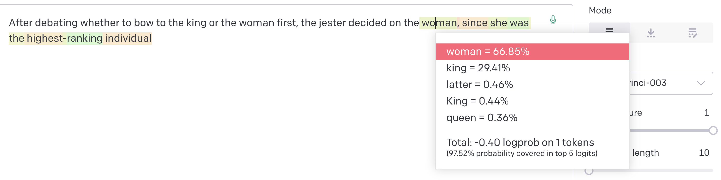
(a) The example where the next word should be either woman or king (or their synonym such as former and latter).

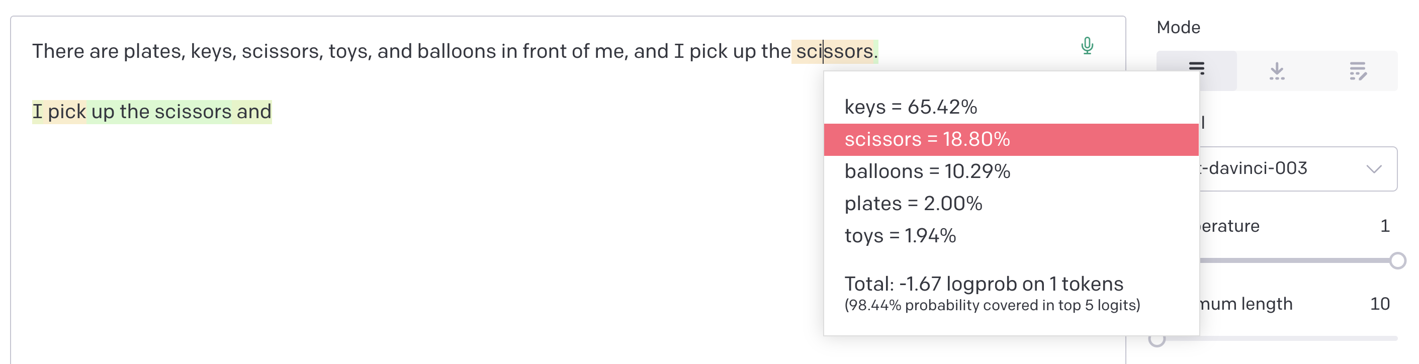
(b) The example where the next word plates, keys, scissors, toys, and balloons should receive similar probabilities.

(c) The example where the next word John, Alex, Mary, Kathryn, and Jack should receive similar probabilities.

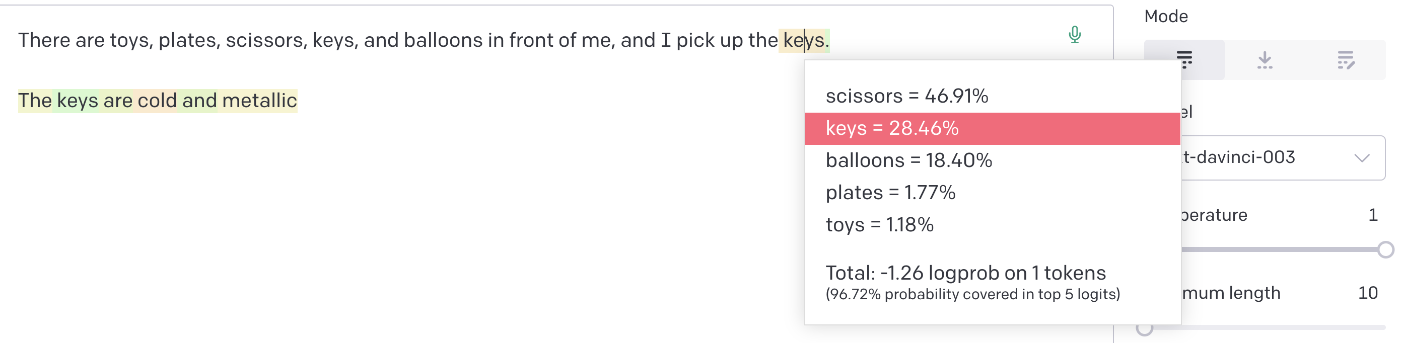
(d) Same as above except that the order of the objects in the context is different.

Figure 4: The next word probabilities outputted by GPT-3.5 (text-davinci-003).

8 Limitations

In our experiments, we find that the improvement of our methods tend to be larger in relatively smaller language models. Due to our limited access of computational resources, we are not able to try our methods on larger LMs. To know if a larger LM still suffers from the softmax bottleneck problem, we input the examples we used in Table 5 to GPT-3.5 and report their results in Figure 4.

We find that although GPT-3.5 greatly reduces the chance of hallucination compared to GPT-2, the next word distribution is still not ideal. For example, in 4(a), although the incorrect answer queen receives only a small probability, GPT-3.5 puts around 67% probability on woman. Similarly, even though GPT-3.5 is unlikely to hallucinate the sentence: There are plates, keys, scissors, toys, and balloons in front of me, and I pick up the phone as GPT-2, 4(b) and 4(d) show that the output distribution is still heavily biased toward one of the options and the most likely next word could change if the order of the options in the context changes. These results suggest that increasing model size indeed alleviates the softmax bottleneck problem but the problem is not completely solved even if a huge hidden state size (12k) and model size (175B) are used (Brown et al., 2020). We expect that adding our methods to the large LMs could rectify the biased distributions as shown in our experiments on smaller LMs (Table 5). Therefore, although improving smaller LMs has already had wide applications in practice, trying our methods on a larger LM is a promising next step, which we haven’t been able to do.

The current implementation of our methods also has some room for improvements. Our codes currently contain some unnecessary computation to circumvent the restrictions of PyTorch library, so we should be able to further accelerate it by writing CUDA code. Furthermore, our codes haven’t supported the pretraining of BART or T5. We expect that completing the future work could make our method faster and better.

Since the focus of this paper is improving the architecture of general transformer decoder, our evaluation of each application is not as comprehensive as the studies for a particular application. For example, although we test our methods using many metrics and the metrics show a consistent trend, there are many other factuality metrics we haven’t tried (Li et al., 2022). We also haven’t conducted human evaluation to further verify our conclusion because conducting human evaluation properly is challenging (Karpinska et al., 2021) and time-consuming. In addition, if we include more words in a context partition, the performance might be better at the cost of extra computational overhead. We leave the analyses of the tradeoff as future work.

9 Ethics Statement

In our experiments, we find that our methods usually copy more words from the context or encoder input. The tendency might have some potential issues. For example, our improvements might be reduced on the languages with more morphology. Furthermore, in some summarization applications, increasing the factuality by increasing the extractiveness might not be ideal (Ladhak et al., 2022; Goyal et al., 2022a).

As described in Section 2.1, one major limitation of the popular softmax layer is its global word embeddings. The problem would become more serious when there are more tokens whose meanings are locally defined (e.g., names in the BookSum dataset). Our methods would be more useful in those circumstances and might alleviate some biases described in Shwartz et al. (2020) and Ladhak et al. (2023). Moreover, the meaning of tokens are also locally defined in many other applications such as variables in code or math problems, the new terminologies in a scientific paper, or the products in a sequential recommendation problem. We believe that our methods could become an efficient alternative of reranker (Cobbe et al., 2021; Welleck et al., 2022) and create impacts in those areas.

Finally, our results show that when there are some uncertainties in the next word (e.g., could be king or woman), existing LMs could have some difficulties of copying the words from the context and our methods alleviate the problem. Thus, our methods should also be able to improve the lexically controllable language generation models that put the desired keywords into the context such as Goldfarb-Tarrant et al. (2019) and Lu et al. (2021).

Appendix A Appendix Overview

In the appendix, we first analyze our methods using more metrics in Appendix B and describe what we learn from the results. Next, we provide some details of our methods and baselines in Appendix C. Finally, we specify some experiment setups and hyperparameters in Appendix D.

	Diagonal (e.g., king or woman)					Edge (e.g., king or queen)
Analogy Relation Types $\rightarrow$		capital-	capital-	city-in-	family		capital-	capital-	city-in-	family
Models $\downarrow$	valid	common	world	state		valid	common	world	state
Softmax + Mi	2.27	3.36	1.94	2.32	3.09	2.13	2.61	1.90	2.21	2.49
MoS + Mi (Chang and McCallum, 2022)	1.86	2.62	1.66	1.86	3.59	1.87	2.24	1.66	1.90	3.10
Softmax + C + Mi	1.78	2.19	1.62	1.87	2.17	1.79	2.13	1.63	1.88	2.07
Softmax + CPR:20,100 + Mi	1.69	2.03	1.54	1.81	2.09	1.69	2.01	1.55	1.81	1.97

Table 7: Comparing the perplexity of different GPT-2 Small models using the synthetic dataset from Chang and McCallum (2022).

Appendix B More Results and Analysis

In this section, we will report more results and provide more detailed analyses accordingly to investigate the advantages of different methods.

Model Name	R1	R1C	R1P	R1PC	R2	P Ratio	CIDEr	NIST
Softmax (GPT-2)	22.668	23.548	7.323	14.340	3.219	0.885	0.182	1.792
Softmax + Mi	22.903	24.036	7.493	14.840	3.289	0.877	0.190	1.829
Mixture of Softmax (MoS) (Yang et al., 2018)	22.965	24.233	7.760	15.762	3.260	0.885	0.188	1.846
MoS + Mi (Chang and McCallum, 2022)	22.876	23.979	7.703	15.493	3.270	0.889	0.188	1.829
Pointer Generator (PG) (See et al., 2017)	23.055	24.872	8.052	17.830	3.311	0.889	0.193	1.856
Pointer Sentinel (PS) (Merity et al., 2017)	23.007	24.444	7.677	16.146	3.302	0.873	0.189	1.840
Softmax + R:20 + Mi	22.941	23.970	7.467	14.733	3.303	0.896	0.188	1.833
Softmax + R:20,100 + Mi	22.909	23.938	7.537	15.066	3.280	0.870	0.190	1.829
Softmax + C + Mi	23.116	25.027	7.894	17.048	3.372	0.917	0.197	1.873
Softmax + P + Mi	23.015	25.080	7.895	17.184	3.346	0.877	0.196	1.847
PG + Mi	22.827	24.759	8.049	17.874	3.289	0.914	0.191	1.819
PS + Mi	22.846	25.008	8.159	18.208	3.307	0.921	0.194	1.823
Softmax + CR:20,100 + Mi	23.017	25.056	8.089	17.798	3.328	0.894	0.198	1.858
Softmax + CPR:20,100 + Mi	23.053	25.361	8.160	17.921	3.363	0.882	0.197	1.863
MoS + CPR:20,100 + Mi	23.047	25.173	8.187	18.198	3.314	0.902	0.198	1.868

Table 8: Comparison of the continuation generated by GPT-2 Small in Wikipedia test data. Table 4 is a short summary of this table. The meaning of the metrics is described in Section B.1. Higher R1C and R1PC mean copying more words from the context. A higher P Ratio means generating more proper nouns. All ROUGE scores are percentages.

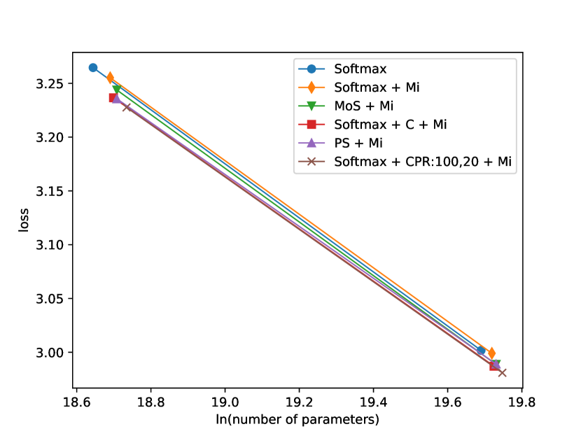
Figure 5: The model size versus the model loss in Wikipedia test data after training for 0.4 epochs. The left side points are the results from GPT-2 Small and the right side points come from GPT-2 Medium. The lower curves are better.

B.1 GPT-2 Experiments

Kaplan et al. (2020); Henighan et al. (2020) demonstrate that the loss decreases linearly as the log of the model size increases. Therefore, a new architecture needs to perform better than the old architecture with a similar model size to verify that the improvement does not come from memorizing more information through the extra parameters. From the loss versus log(model size) curve in Figure 5, we can see that our proposed methods are significantly better than MoS and slightly better than a pointer network baseline as the model becomes larger.

We use the following metrics to measure the text generated by GPT-2.

• ROUGE-1 (R1): The prediction F1 for unigram in the actual continuation.

• ROUGE-1 Context (R1C): The prediction F1 for unigram in the context.

• ROUGE-1 Proper (R1P): The same as ROUGE-1 except that only the proper nouns are considered. We measure this metric because the correctness of the entity name prediction is critical to the factuality of the generation.

• ROUGE-1 Proper Context (R1PC): The same as ROUGE-1 Context (R1C) except that only the proper nouns are considered.

• ROUGE-2 (R2): The prediction F1 for bigram in the actual continuation.

• Proper Noun Ratio (P Ratio): The average number of proper nouns in the generation divided by the average number of proper nouns in the actual continuation. The LMs usually generate fewer proper nouns compared to the actual continuation (See et al., 2019), so the values are usually lower than 1. The P Ratio closer to 1 is better.

• CIDEr (Vedantam et al., 2015): A metric for measuring the quality and specificity of the generation.

• NIST (Doddington, 2002): Similar to CIDEr. CIDEr uses tf-idf to weigh the n-gram while NIST measures the information gain.

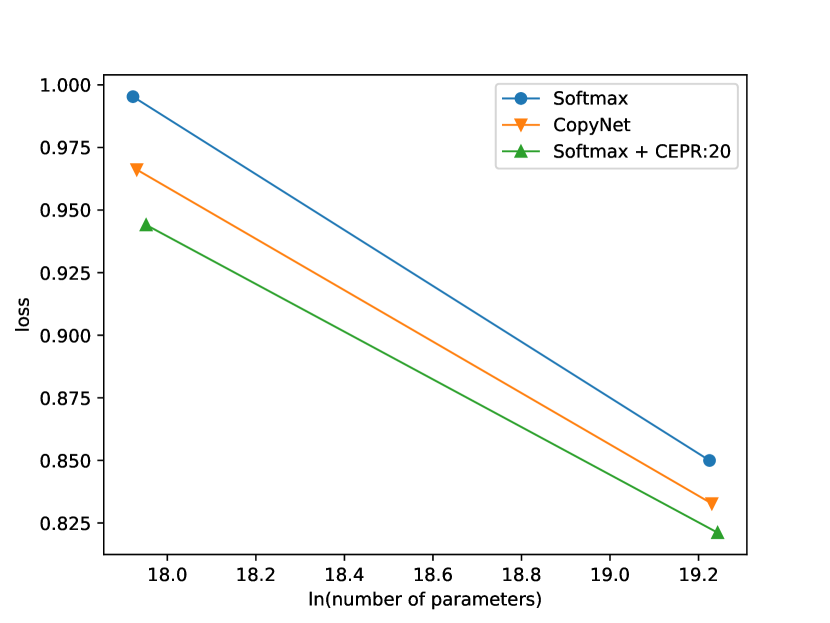
Figure 6: The model size versus the model loss in CNN/DM test set. The left side points are the results from T5-Small and the right side points come from T5-Base. The lower curves are better.

The results are reported in Table 8. In terms of R1, R2, CIDEr, and NIST, our proposed methods such as Softmax + C + Mi and Softmax + CPR:20,100 + Mi are significantly better than the pointer network baselines PS + Mi and PG + Mi. Comparing with Softmax + CPR:20,100 + Mi, PS + Mi has a significantly higher P Ratio and R1PC but similar R1P. This indicates that PS + Mi copies more proper nouns from the context while there is a similar number of proper nouns that are in actual continuation, so Softmax + CPR:20,100 + Mi actually has a higher accuracy on the proper noun prediction.

In text corpus such as Wikipedia, we do not know the ground truth next word distribution and which context leads to multiple probable next words, so we cannot quantitatively analyze the improvement on the ambiguous contexts. To alleviate the concern, we test our methods on the synthetic dataset constructed by Chang and McCallum (2022). The dataset is built using templates and Google analogy dataset (Mikolov et al., 2013), so we know the ground truth next word distribution. The dataset consists of the ambiguous contexts such as I went to Paris and Germany before, and I love one of the places more, which is, where the next word is either the diagonal words of the parallelogram such as Paris and Germany or the edge words such as Paris and France. For the details of the experimental setup, please refer to Chang and McCallum (2022).

In Table 7, we can see that Softmax + CPR:20,100 + Mi achieves the lowest perplexity in all subsets and outperforms the Softmax + Mi baseline by a large margin, especially in the diagonal subset where the ground truth word embedding distribution has multiple modes. Notice that the performance of MoS + Mi is worse than what reported in Chang and McCallum (2022) probably because we shared the input and output word embeddings.

		CNN/DM					XSUM
Models	Size	Loss ($\downarrow$)	R2	R1P	P Ratio	NIST	Loss ($\downarrow$)	R2	R1P	P Ratio	NIST
T5-Small
Softmax (S)	60.8M	0.995	15.147	0.462	0.915	4.650	0.538	7.098	0.292	0.853	2.738
CopyNet (Gu et al., 2016)	61.3M	0.966	14.942	0.458	0.985	4.607	0.533	7.055	0.286	0.865	2.742
PG (See et al., 2017)	61.3M	0.978	14.789	0.453	0.943	4.589	0.535	7.211	0.288	0.849	2.744
PS (Merity et al., 2017)	61.3M	0.970	14.866	0.455	0.946	4.629	0.535	7.000	0.283	0.853	2.718
S + R:20	61.0M	0.985	14.831	0.456	0.928	4.603	0.534	7.085	0.287	0.858	2.730
S + E	61.0M	0.956	14.935	0.457	0.950	4.629	0.530	7.152	0.292	0.864	2.759
S + CE	61.3M	0.954	15.124	0.462	0.956	4.691	0.528	7.304	0.297	0.873	2.815
S + CER:20	61.5M	0.953	14.996	0.463	0.953	4.667	0.527	7.194	0.296	0.871	2.800
S + CEPR:20	62.6M	0.944	15.194	0.476	0.971	4.739	0.525	7.363	0.305	0.878	2.844
S + CEPR:20 + Mi	65.5M	0.943	15.094	0.471	0.976	4.720	0.523	7.340	0.305	0.874	2.840
T5-Base
Softmax (S)	223.5M	0.850	16.410	0.491	0.959	4.948	0.417	10.773	0.386	0.910	3.454
CopyNet (Gu et al., 2016)	224.7M	0.833	16.253	0.486	0.979	4.915	0.416	10.804	0.387	0.915	3.467
PG (See et al., 2017)	224.7M	0.840	16.134	0.485	0.955	4.923	0.417	10.815	0.389	0.915	3.466
PS (Merity et al., 2017)	224.7M	0.836	16.275	0.490	0.978	4.908	0.417	10.838	0.386	0.915	3.473
S + CEPR:20	227.6M	0.821	16.292	0.497	0.990	4.966	0.412	10.778	0.389	0.930	3.477
S + CEPR:20 + Mi	234.1M	0.821	16.457	0.499	0.987	4.997	0.412	10.921	0.391	0.929	3.511
BART Base
Softmax (S)	140.0M	0.874	15.613	0.471	1.028	4.641	0.391	12.944	0.428	0.928	3.833
CopyNet (Gu et al., 2016)	141.2M	0.837	15.675	0.470	1.013	4.685	0.387	12.740	0.424	0.934	3.818
PG (See et al., 2017)	141.2M	0.845	15.485	0.465	1.018	4.669	0.389	12.849	0.425	0.928	3.827
PS (Merity et al., 2017)	141.2M	0.838	15.689	0.468	0.996	4.750	0.387	12.690	0.423	0.926	3.796
S + R:20	140.6M	0.863	15.486	0.468	1.028	4.655	0.389	12.804	0.426	0.941	3.824
S + E	140.6M	0.852	15.412	0.466	1.018	4.652	0.389	12.893	0.428	0.933	3.844
S + CE	141.2M	0.851	15.555	0.471	1.013	4.692	0.388	12.830	0.426	0.934	3.827
S + CER:20	141.8M	0.850	15.550	0.469	1.022	4.672	0.387	12.787	0.423	0.940	3.821
S + CEPR:20	144.1M	0.841	15.778	0.471	1.025	4.724	0.387	12.824	0.423	0.942	3.829
S + CEPR:20 + Mi	150.6M	0.843	15.632	0.472	1.027	4.700	0.387	12.969	0.426	0.939	3.847
BART Large
Softmax (S)	407.3M	0.794	16.386	0.488	1.091	4.654	0.359	15.386	0.476	1.006	4.136
CopyNet (Gu et al., 2016)	409.4M	0.774	16.268	0.485	1.113	4.619	0.358	15.293	0.473	0.995	4.144
PG (See et al., 2017)	409.4M	0.780	16.344	0.486	1.097	4.656	0.358	15.544	0.475	0.995	4.186
PS (Merity et al., 2017)	409.4M	0.774	16.142	0.484	1.099	4.654	0.358	15.547	0.475	1.000	4.227
S + CEPR:20	414.7M	0.780	16.394	0.488	1.073	4.767	0.359	15.466	0.476	0.982	4.240
S + CEPR:20 + Mi	426.2M	0.769	16.085	0.483	1.032	4.811	0.347	15.371	0.475	0.957	4.292

Table 9: Comparison of the summaries generated by different models in the test sets of CNN/DM and XSUM datasets. We also report the number of parameters of each model. From top to bottom, the four sections are the results of T5-Small, T5-Base, BART Base, and BART Large. The meaning of the metrics are described in Section B.1. R2 (ROUGE 2-F1) scores are percentages. Within each section, we highlight the smallest loss, the P Ratio that is closest to 1, and highest numbers in the other metrics.

		BookSum Paragraph					SAMSUM
Models	Time (ms)	Loss ($\downarrow$)	R2	R1P	P Ratio	NIST	Loss ($\downarrow$)	R2	R1P	P Ratio	NIST
T5-Small
Softmax (S)	30.1	0.654	1.673	0.149	0.589	1.383	0.383	13.806	0.605	0.873	3.945
CopyNet (Gu et al., 2016)	37.0	0.646	1.722	0.183	0.747	1.440	0.381	14.210	0.594	0.809	3.965
PG (See et al., 2017)	43.4	0.648	1.669	0.160	0.631	1.413	0.392	10.673	0.542	0.711	1.665
PS (Merity et al., 2017)	37.6	0.646	1.627	0.177	0.700	1.417	0.383	13.817	0.583	0.794	3.960
S + R:20	32.9	0.652	1.663	0.159	0.677	1.403	0.380	13.728	0.598	0.870	3.995
S + E	33.8	0.645	1.710	0.171	0.673	1.421	0.370	13.557	0.602	0.892	3.906
S + CE	34.0	0.644	1.734	0.173	0.680	1.436	0.368	14.136	0.619	0.892	3.971
S + CER:20	35.8	0.642	1.710	0.174	0.693	1.434	0.367	14.281	0.627	0.911	3.968
S + CEPR:20	38.4	0.641	1.768	0.184	0.725	1.461	0.365	14.451	0.639	0.909	4.034
S + CEPR:20 + Mi	41.7	0.641	1.733	0.185	0.721	1.458	0.365	14.193	0.630	0.922	4.011
T5-Base
Softmax (S)	102.4	0.587	1.876	0.160	0.650	1.443	0.308	17.662	0.672	0.915	4.559
CopyNet (Gu et al., 2016)	110.3	0.582	1.867	0.187	0.744	1.481	0.307	17.556	0.678	0.901	4.544
PG (See et al., 2017)	117.7	0.585	1.832	0.159	0.647	1.434	0.317	14.649	0.611	0.740	1.870
PS (Merity et al., 2017)	112.0	0.582	1.899	0.176	0.718	1.465	0.308	17.502	0.660	0.897	4.453
S + CEPR:20	115.3	0.580	1.842	0.191	0.771	1.482	0.300	18.082	0.677	0.950	4.553
S + CEPR:20 + Mi	116.3	0.584	1.860	0.187	0.770	1.477	0.301	17.617	0.677	0.938	4.521
BART Base
Softmax (S)	46.6	0.624	1.807	0.141	0.656	1.425	0.327	19.379	0.672	0.995	4.546
CopyNet (Gu et al., 2016)	57.8	0.613	1.866	0.166	0.728	1.454	0.326	18.227	0.662	0.944	4.535
PG (See et al., 2017)	64.8	0.624	1.864	0.140	0.668	1.428	0.328	18.791	0.673	0.963	4.537
PS (Merity et al., 2017)	57.9	0.613	1.867	0.163	0.723	1.461	0.324	18.367	0.674	0.951	4.573
S + R:20	50.5	0.627	1.807	0.154	0.720	1.430	0.326	19.022	0.671	0.971	4.608
S + E	54.2	0.620	1.825	0.150	0.688	1.429	0.324	18.902	0.680	0.970	4.501
S + CE	56.5	0.619	1.847	0.153	0.685	1.441	0.323	18.739	0.672	0.949	4.537
S + CER:20	57.2	0.618	1.834	0.156	0.727	1.444	0.321	19.267	0.678	0.981	4.561
S + CEPR:20	58.8	0.618	1.865	0.157	0.742	1.457	0.321	18.631	0.670	0.992	4.516
S + CEPR:20 + Mi	63.2	0.620	1.827	0.158	0.733	1.442	0.322	18.681	0.670	0.987	4.439
BART Large
Softmax (S)	143.5	0.554	2.094	0.171	0.722	1.472	0.303	20.848	0.711	1.006	4.621
CopyNet (Gu et al., 2016)	168.9	0.548	2.087	0.184	0.762	1.490	0.298	21.703	0.708	1.026	4.727
PG (See et al., 2017)	178.3	0.731	2.090	0.174	0.725	1.479	0.301	21.428	0.706	1.051	4.604
PS (Merity et al., 2017)	168.5	0.726	2.083	0.184	0.760	1.493	0.300	22.144	0.710	1.036	4.779
S + CEPR:20	169.9	0.552	2.069	0.178	0.763	1.505	0.302	21.326	0.691	1.017	4.595
S + CEPR:20 + Mi	177.4	0.544	2.024	0.175	0.737	1.500	0.294	21.244	0.713	0.959	4.746

Table 10: Comparison of the summaries generated by different models in the test sets of BookSum and SAMSUM datasets. We also report the inference time of one samples. The meaning of the metrics are described in Section B.1. R2 (ROUGE 2-F1) scores are percentages. Within each section, we highlight the smallest loss, the P Ratio that is closest to 1, and highest numbers in the other metrics.

B.2 Summarization

Compared to Figure 5, Figure 6 shows that our methods improve the loss of T5 in CNN/DM more than GPT-2 in Wikipedia.

In Table 9 and Table 10, we compare the different summarization models by their model size, evaluation losses, inference time, and other metrics which we use in subsection B.1. The pointer network baselines and our methods significantly improve most metrics over the softmax baseline, which is used ubiquitously in nearly all LMs. Although our method generally improves less on the T5-Base model, the percentages of additional parameters and inference time overhead are much smaller. Although our methods tend to improve less in larger language model, we still improve BART Large very significantly in NIST, CIDEr, and MAUVE, and Mi seems to become more effective in BART Large.

The testing set of SAMSUM dataset only has 819 samples, so some metrics such as R1 and R2 are not as stable as other three datasets. PG (See et al., 2017) for T5-Small and T5-Base perform much worse in SAMSUM dataset. We hypothesize that it is because the dialog input in SAMSUM dataset is very different from the pretraining data of T5, which makes training PG unstable.

In most datasets and models, the R Ratio from our method is significantly closer to 1 than the softmax baseline, which means the average number of proper nouns in our summaries is much closer to the average number of proper nouns in the human-written summary. For example, in BookSum Paragraph, we improve its R Ratio by 26%, which partially explains our large MAUVE improvement in Table 6. Notice that our methods do not always output more proper nouns. For example, for BART Base in CNN/DM dataset, our methods reduce the R Ratio of the softmax baseline, which is larger than 1. This shows that our methods could learn when we should copy the proper nouns according to the training data.

Appendix C Method Details

We describe some details of our methods and baselines in this section.

C.1 Proposed Methods

To allow us to start from existing LMs that are pretrained using softmax, we keep the modified softmax layer initially working almost the same as the original softmax layer. We initialize the linear transformation weights of $L_{PD}^{f}()$, $L_{LD}^{f}()$, $L_{PE}^{f}()$, and $L_{LE}^{f}()$ as $10^{-10}\cdot\mathbb{I}$. The other linear weights $L_{.}^{f}()$ are initialized as the identity matrix $\mathbb{I}$.

In the local decoder embedding method Softmax + P + Mi, the initialization would give the 0 logit to all context words. To solve the issue, we revise Equation 3 a little and compute $\text{Logit}_{P}(x,c_{t})$ by

$$\left\{\begin{matrix}[l]{\bm{f}}_{c_{t},V}^{T}{\bm{w}}_{x}+{\bm{f}}_{c_{t},PD}^{T}{\bm{f}}_{x,c_{t},LD}\;\;\text{if}\;x\in c_{t}\\ {\bm{f}}_{c_{t},V}^{T}{\bm{w}}_{x}\;\;\text{O/W}\end{matrix}\right..$$ (7)

That is, we initially rely on the original softmax layer to compute all the logits and let the term ${\bm{f}}_{c_{t},PD}^{T}{\bm{f}}_{x,c_{t},LD}$ gradually influences the logits of the context words.

In MoS + CPR:20,100 + Mi, our proposed method only revises the logit in one of the softmax.

C.2 Pointer Network Baselines

The pointer networks are originally designed for RNN, so we are unable to use exactly the same formula proposed in the papers. Nevertheless, we try our best to adapt the pointer networks for the transformer encoder while keeping the gist of the formulas. In all methods, to let the results more comparable to our methods, we use ${\bm{f}}_{c_{t},PE}$ and $L_{LE}^{f}$ to determine the probability of copying the words from the context, and use ${\bm{f}}_{c_{t},V}^{T}{\bm{w}}_{x}$ to determine the probability of generating all the words in the vocabulary.

In CopyNet (Gu et al., 2016), we compute the probability of outputting the word $x$ as

$$Prob(x|I,c_{t})\propto\text{exp}\left({\bm{f}}_{c_{t},V}^{T}{\bm{w}}_{x}\right)$$

$$+\sum_{j=1}^{|I|}\mathbbm{1}_{{I^{j}}=x}\text{exp}\left({\bm{f}}_{c_{t},PE}^{T}L_{LE}^{f}({\bm{h}}_{I^{j}}^{M})+b\right).$$ (8)

Notice that CopyNet needs to sum up the exponential of dot products, which often causes overflow problems in GPT-2. We can set $b$ to be a large negative value initially to solve the problem, but its perplexity is much worse than the other two pointer network variants. Thus, we choose to skip the CopyNet in the GPT-2 experiments.

In Pointer Generator (See et al., 2017), we compute the probability of $x$ using

$$Prob(x|I,c_{t})=p_{gen}\frac{\text{exp}\left({\bm{f}}_{c_{t},V}^{T}{\bm{w}}_{x}\right)}{Z_{V}}$$

$$+(1-p_{gen})\sum_{j=1}^{|I|}\mathbbm{1}_{{I^{j}}=x}P_{E}(j|I,c_{t}),$$ (9)

where $P_{E}(j|I,c_{t})=\frac{\text{exp}\left({\bm{v}}^{T}\text{tanh}({\bm{f}}_{c_{t},PE}+L_{LE}^{f}({\bm{h}}_{I^{j}}^{M})+{\bm{b}})\right)}{Z_{E}}$, $p_{gen}=\sigma({\bm{q}}^{T}{\bm{h}}_{c_{t}}^{M}+b_{ptr})$, the normalization term $Z_{V}=\sum_{x\in V}\text{exp}\left({\bm{f}}_{c_{t},V}^{T}{\bm{w}}_{x}\right)$, and $Z_{E}=\sum\limits_{j=1}^{|I|}\text{exp}\left({\bm{v}}^{T}\text{tanh}({\bm{f}}_{c_{t},PE}+L_{LE}^{f}({\bm{h}}_{I^{j}}^{M})+{\bm{b}})\right)$.

We skip the coverage mechanism in the pointer generator paper to make it more comparable to other methods. In T5 experiments, its training loss is sometimes very large, so we set $b_{ptr}$ as 3 initially to keep the $p_{gen}$ close to 1 (i.e., turn pointer part off initially). In other experiments, we set $b_{ptr}=0$.

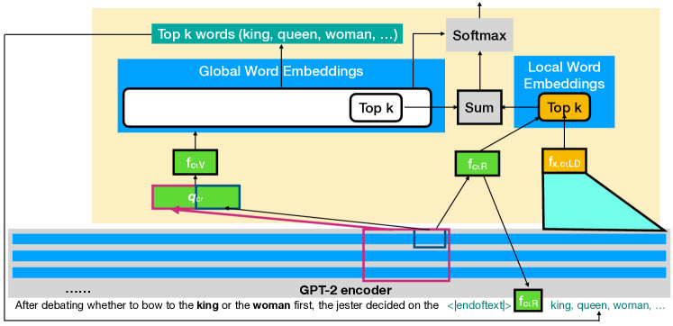
Figure 7: Word-by-word reranker architecture.

Figure 8: Our efficient implementation of word-by-word reranker. Ti is tokens and ki.j is top-k tokens for Ti.

In Pointer Sentinel (Merity et al., 2017), the probability of $x$ is computed by

$$Prob(x|I,c_{t})=g\frac{\text{exp}\left({\bm{f}}_{c_{t},V}^{T}{\bm{w}}_{x}\right)}{Z_{V}}$$

$$+\sum_{j=1}^{|I|}\mathbbm{1}_{{I^{j}}=x}\frac{\text{exp}\left({\bm{f}}_{c_{t},PE}^{T}\text{tanh}(L_{LE}^{f}({\bm{h}}_{I^{j}}^{M}))+b\right)}{Z_{p}},$$ (10)

$g=\frac{\text{exp}({\bm{q}}^{T}{\bm{h}}_{c_{t}}^{M})}{Z_{p}}$, and $Z_{p}=\text{exp}({\bm{q}}^{T}{\bm{h}}_{c_{t}}^{M})+\sum_{j=1}^{|I|}\text{exp}\left({\bm{f}}_{c_{t},PE}^{T}\text{tanh}(L_{LE}^{f}({\bm{h}}_{I^{j}}^{M}))+b\right)$.

In our experiments, we find that the pointer network variants usually have similar performance (except that PG sometimes performs much worse in summarization due to some training stability issues). This suggests that the differences in the pointer network variants often do not influence the performance significantly, which justifies our simplification of the formulas in the original paper and supports our conclusion that the improvement comes from breaking the softmax bottleneck.

Notice that in the above pointer network variants, the pointer part can only increase the probability of the context words from the generator part. As a result, it cannot alleviate the repetition problem in the last example of Table 5.

C.3 Word-by-word Reranker Baseline

We illustrate our word-by-word reranker (wbwR) in Figure 7. The method has two stages. In the first stage, we compute the logits using the projected hidden state ${\bm{f}}_{c_{t},V}$ and retrieve the top $k$ words. At the second stage, we append the top $k$ words to the input context along with the hidden state ${\bm{f}}_{c_{t},R}$ for reranking the context words. We use the same positional embeddings for all candidates to encourage the model to change the ranking of the words. Next, we use the hidden states corresponding to the candidates to compute their local word embeddings as ${\bm{f}}_{x,c_{t},LD}$. Finally, we re-estimate the probabilities of top $k$ words by

$$\left\{\begin{matrix}[l]{\bm{f}}_{c_{t},V}^{T}{\bm{w}}_{x}+{\bm{f}}_{c_{t},R}^{T}{\bm{f}}_{x,c_{t},LD}\;\;\text{if}\;x\in W(k)\\ {\bm{f}}_{c_{t},V}^{T}{\bm{w}}_{x}\;\;\text{O/W}\end{matrix}\right..$$ (11)

To improve the quality of our top k candidates, the final loss is the addition of the wbwR loss at the second stage and the loss of the original softmax layer that only uses the logits from ${\bm{f}}_{c_{t},V}^{T}{\bm{w}}_{x}$ at the first stage. When we combine the wbwR with Softmax + CPR:20,100 + Mi, we simply use Softmax + CPR:20,100 + Mi at the first stage and use the wbwR to overwrite the logits of Softmax + CPR:20,100 + Mi at the second stage.

Using this method, we can update the embeddings of the words that are not in the context and allow the candidates to interact with the input context to determine their probabilities as the classic two-stage reranker while keeping the model size roughly unchanged. Nevertheless, the method can only change the probability of the top $k$ words and its computational overhead and memory requirement prevents us from using a very large $k$.

Unlike the standard GPT-2, we cannot get the probability of all positions in one forward pass because the input contexts are different when computing the probability at each position and the input of the second stage reranker depends on the results of the previous forward pass at the first stage. To speed up, we reuse the computed hidden states and batchify the forward passes.

In our implementation, we first get the top $k$ candidates corresponding to all tokens in the stage1 (just original GPT2) as the input of stage2 reranker. To avoid recalculating the hidden states of the context at stage2, we store the hidden states using the past-key-value in Hugging Face and only compute the hidden states corresponding to the top $k$ candidate tokens at stage2.

We divide the computation of the whole input sequence into several blocks as shown in Figure 8. In each block, we input a batch containing the last few tokens and top $k$ candidates into the GPT-2 while reusing the hidden states of their common contexts from stage1. In this way, we can increase parallelism by increasing the block size if the GPU memory allows it.

Even though we spent substantial effort on optimizing the wbwR, the method is still too slow to be practically useful. Even if we use four RTX 8000 (a faster GPU with a larger memory), our wbwR implementation is still around 10 times slower than our proposed Softmax + CPR:20,100 + Mi that uses only one RTX 2080.

Appendix D Experiment Details

For the reproducibility, we provide some experimental configuration in this section. Please see our codes (https://github.com/iesl/Softmax-CPR) for more details.

D.1 GPT-2 Experimental Details

We mostly follow the experimental setup Chang and McCallum (2022) except that we share the input and output word embeddings as in the standard GPT-2 models. As in Chang and McCallum (2022), we use the last 2% of the corpus as the test set and the 2% before that as the validation set. In the word-by-word reranking experiment, we only use first 100k tokens in validation set to speed up the evaluation. To show that our model could be added to existing pretrained models, we continue training the pretrained GPT-2. For GPT-2 Small, we train for $1$ epoch, and for GPT-2 Medium, we train for $0.4$ epoch. We find that the performance improvements usually do not change significantly after training for $0.1$ epoch.

As in Chang and McCallum (2022), we set the sequence length as $200$, batch size as $4$, and learning rate for AdamW as $1e-5$. Our methods only have two hyperparameters, $k_{1}$ and $k_{2}$, and we try values $20$, $100$, $200$, $500$ and select $20$ and $100$ using the validation data.

In the text completion experiment, we generate $360$k continuations with a length of $50$ given the prompts in Wikipedia. We first sample $40$k sequences in the test data of Wikipedia 2021. Next, we use the first $20$, $70$, and $120$ words in the sequence as our context and let the different models generate the next $50$ words as continuations. The references are the actual next $50$ words. All the methods use Top-K sampling and K=$5$.

	Train	Val	Test
CNN/DM	287113	13368	11490
XSUM	204045	11332	11334
BookSum Paragraph	210931	27222	26025
SAMSUM	14732	818	819

Table 11: Dataset size of our four summarization tasks.

D.2 Summarization Experimental Details

BookSum dataset (Kryściński et al., 2021) includes three summarization tasks: Summarizing a book, a chapter, and a paragraph. We test our methods using the paragraph summarization task due to the input length restriction of BART and T5. The dataset is constructed by automatically aligning the paragraphs in a chapter with the sentences in a chapter summary, which introduces noise to the dataset. Similarly, XSUM uses the first sentence in news instead of manually-written summary as the ground truth reference. The relatively noisier datasets such as XSUM and BookSum Paragraph, and smaller dataset like SAMSUM could test the stability of the methods. The sizes of the summarization datasets could be found in Table 11.

We conduct the summarization experiments based on a summarization example code from Hugging Face. Most of our hyperparameters use the default value in the code. In our preliminary study, our improvement is not sensitive to the hyperparameter choice (e.g., the improvement gap is similar across different numbers of epochs). Thus, we do not tune the hyperparameters for each method or for each dataset unless we cannot reach a low training loss at the end.

In CNN/DM, XSUM, and SAMSUM datasets, We train models for $3$ epochs. In BookSum datasets, We trained models for $5$ epochs. The learning rate is set to be $5e-05$ except for BART Large model in BookSum, where we use $1e-05$ to stablize the training of all methods.

All the experiments use batch size 8 and AdamW with betas=($0.9$,$0.999$), epsilon=$1e-06$, weight-decay=$1.2e-6$. During the generation, we used Top-K sampling (K=$10$) as our decoding method. The maximum summary length is set as $128$ and maximum input length is $1024$. We use warmup for the first $1000$ steps in all the experiments, which allows us to change the architecture of T5 and BART more significantly (e.g., using Mi) without having a training stability issue.

The $k$ in the reranker partition and the block size of multiple input hidden states (Mi) is coarsely tuned based on validation performance of CNN/DM. Unlike considering the top $100$ words in the open-end text completion using GPT-2, we find that reranking the top $20$ words is sufficient for our summarization models, probably because next words are easier to predict in the summarization task.

For our evaluation metrics, we use the default setting for ROUGE and set use_stemmer=True. When reporting the ROUGE scores, we follow the conventions to show their percentages. We use the default setting for MAUVE, CIDER, NIST. For MAUVE, we insert a new line symbol after every sentence as in the original Hugging Face summarization example code. For factCC metric, we use the author-provided checkpoint to evaluate CNN/DM results since factCC is originally trained in CNN/DM. For the other three summarization datasets, we follow the author’s codes to constructed positive and negative data and continued training the CNN/DM factCC model on each dataset with one epoch respectively. Then we evaluate different summarization tasks with the corresponding factCC checkpoint.

D.3 Computational Environment and Software

We implement our methods by revising the Hugging Face library Wolf et al. (2020). From Hugging Face, we load the pretrained LMs including GPT-2 Small, GPT-2 Medium, T5-Small, T5-Base, BART Base, and BART Large. We use SpaCy (Honnibal et al., 2020) to detect the proper nouns.

For GPT-2 Medium, T5-Base, and BART Large, we use NVIDIA GeForce RTX 8000 to train the model and for other smaller models, we use NVIDIA GeForce RTX 2080. Most of experiments could be done within one week. In all the inference time experiments, we use NVIDIA GeForce GTX TITAN X, batch size 4 for GPT-2, and batch size 8 for BART and T5.

References

- Adolphs et al. (2022) Leonard Adolphs, Tianyu Gao, Jing Xu, Kurt Shuster, Sainbayar Sukhbaatar, and Jason Weston. 2022. The cringe loss: Learning what language not to model. ArXiv preprint, abs/2211.05826.
- An et al. (2022) Chenxin An, Jiangtao Feng, Kai Lv, Lingpeng Kong, Xipeng Qiu, and Xuanjing Huang. 2022. Cont: Contrastive neural text generation. ArXiv preprint, abs/2205.14690.
- Arora et al. (2022) Kushal Arora, Kurt Shuster, Sainbayar Sukhbaatar, and Jason Weston. 2022. Director: Generator-classifiers for supervised language modeling. In Proceedings of the 2nd Conference of the Asia-Pacific Chapter of the Association for Computational Linguistics and the 12th International Joint Conference on Natural Language Processing, pages 512–526.
- Brown et al. (2020) Tom B. Brown, Benjamin Mann, Nick Ryder, Melanie Subbiah, Jared Kaplan, Prafulla Dhariwal, Arvind Neelakantan, Pranav Shyam, Girish Sastry, Amanda Askell, Sandhini Agarwal, Ariel Herbert-Voss, Gretchen Krueger, Tom Henighan, Rewon Child, Aditya Ramesh, Daniel M. Ziegler, Jeffrey Wu, Clemens Winter, Christopher Hesse, Mark Chen, Eric Sigler, Mateusz Litwin, Scott Gray, Benjamin Chess, Jack Clark, Christopher Berner, Sam McCandlish, Alec Radford, Ilya Sutskever, and Dario Amodei. 2020. Language models are few-shot learners. In Advances in Neural Information Processing Systems 33: Annual Conference on Neural Information Processing Systems 2020, NeurIPS 2020, December 6-12, 2020, virtual.
- Cao and Wang (2021) Shuyang Cao and Lu Wang. 2021. CLIFF: Contrastive learning for improving faithfulness and factuality in abstractive summarization. In Proceedings of the 2021 Conference on Empirical Methods in Natural Language Processing, pages 6633–6649, Online and Punta Cana, Dominican Republic. Association for Computational Linguistics.
- Chang and McCallum (2022) Haw-Shiuan Chang and Andrew McCallum. 2022. Softmax bottleneck makes language models unable to represent multi-mode word distributions. In Proceedings of the 60th Annual Meeting of the Association for Computational Linguistics (Volume 1: Long Papers), pages 8048–8073, Dublin, Ireland. Association for Computational Linguistics.
- Cobbe et al. (2021) Karl Cobbe, Vineet Kosaraju, Mohammad Bavarian, Mark Chen, Heewoo Jun, Lukasz Kaiser, Matthias Plappert, Jerry Tworek, Jacob Hilton, Reiichiro Nakano, et al. 2021. Training verifiers to solve math word problems. ArXiv preprint, abs/2110.14168.
- Deng et al. (2020) Yuntian Deng, Anton Bakhtin, Myle Ott, Arthur Szlam, and Marc’Aurelio Ranzato. 2020. Residual energy-based models for text generation. In 8th International Conference on Learning Representations, ICLR 2020, Addis Ababa, Ethiopia, April 26-30, 2020. OpenReview.net.
- Doddington (2002) George Doddington. 2002. Automatic evaluation of machine translation quality using n-gram co-occurrence statistics. In Proceedings of the second international conference on Human Language Technology Research, pages 138–145.
- Gabriel et al. (2021) Saadia Gabriel, Antoine Bosselut, Jeff Da, Ari Holtzman, Jan Buys, Kyle Lo, Asli Celikyilmaz, and Yejin Choi. 2021. Discourse understanding and factual consistency in abstractive summarization. In Proceedings of the 16th Conference of the European Chapter of the Association for Computational Linguistics: Main Volume, pages 435–447, Online. Association for Computational Linguistics.
- Glass et al. (2022) Michael Glass, Gaetano Rossiello, Md Faisal Mahbub Chowdhury, Ankita Naik, Pengshan Cai, and Alfio Gliozzo. 2022. Re2G: Retrieve, rerank, generate. In Proceedings of the 2022 Conference of the North American Chapter of the Association for Computational Linguistics: Human Language Technologies, pages 2701–2715, Seattle, United States. Association for Computational Linguistics.
- Gliwa et al. (2019) Bogdan Gliwa, Iwona Mochol, Maciej Biesek, and Aleksander Wawer. 2019. SAMSum corpus: A human-annotated dialogue dataset for abstractive summarization. In Proceedings of the 2nd Workshop on New Frontiers in Summarization, pages 70–79, Hong Kong, China. Association for Computational Linguistics.
- Goldfarb-Tarrant et al. (2019) Seraphina Goldfarb-Tarrant, Haining Feng, and Nanyun Peng. 2019. Plan, write, and revise: an interactive system for open-domain story generation. In Proceedings of the 2019 Conference of the North American Chapter of the Association for Computational Linguistics (Demonstrations), pages 89–97, Minneapolis, Minnesota. Association for Computational Linguistics.
- Goyal et al. (2022a) Tanya Goyal, Junyi Jessy Li, and Greg Durrett. 2022a. News summarization and evaluation in the era of gpt-3. arXiv preprint arXiv:2209.12356.
- Goyal et al. (2022b) Tanya Goyal, Junyi Jessy Li, and Greg Durrett. 2022b. Snac: Coherence error detection for narrative summarization. ArXiv preprint, abs/2205.09641.
- Gu et al. (2016) Jiatao Gu, Zhengdong Lu, Hang Li, and Victor O.K. Li. 2016. Incorporating copying mechanism in sequence-to-sequence learning. In Proceedings of the 54th Annual Meeting of the Association for Computational Linguistics (Volume 1: Long Papers), pages 1631–1640, Berlin, Germany. Association for Computational Linguistics.
- Guan et al. (2022) Jian Guan, Zhenyu Yang, Rongsheng Zhang, Zhipeng Hu, and Minlie Huang. 2022. Generating coherent narratives by learning dynamic and discrete entity states with a contrastive framework. ArXiv preprint, abs/2208.03985.
- Henighan et al. (2020) Tom Henighan, Jared Kaplan, Mor Katz, Mark Chen, Christopher Hesse, Jacob Jackson, Heewoo Jun, Tom B Brown, Prafulla Dhariwal, Scott Gray, et al. 2020. Scaling laws for autoregressive generative modeling. ArXiv preprint, abs/2010.14701.
- Hochreiter and Schmidhuber (1997) Sepp Hochreiter and Jürgen Schmidhuber. 1997. Long short-term memory. Neural computation, 9(8):1735–1780.
- Honnibal et al. (2020) Matthew Honnibal, Ines Montani, Sofie Van Landeghem, and Adriane Boyd. 2020. spaCy: Industrial-strength Natural Language Processing in Python.
- Jiang et al. (2022a) Dongfu Jiang, Bill Yuchen Lin, and Xiang Ren. 2022a. Pairreranker: Pairwise reranking for natural language generation. arXiv preprint arXiv:2212.10555.
- Jiang et al. (2022b) Shaojie Jiang, Ruqing Zhang, Svitlana Vakulenko, and Maarten de Rijke. 2022b. A simple contrastive learning objective for alleviating neural text degeneration. ArXiv preprint, abs/2205.02517.
- Kaplan et al. (2020) Jared Kaplan, Sam McCandlish, Tom Henighan, Tom B Brown, Benjamin Chess, Rewon Child, Scott Gray, Alec Radford, Jeffrey Wu, and Dario Amodei. 2020. Scaling laws for neural language models. ArXiv preprint, abs/2001.08361.
- Karpinska et al. (2021) Marzena Karpinska, Nader Akoury, and Mohit Iyyer. 2021. The perils of using Mechanical Turk to evaluate open-ended text generation. In Proceedings of the 2021 Conference on Empirical Methods in Natural Language Processing, pages 1265–1285, Online and Punta Cana, Dominican Republic. Association for Computational Linguistics.
- King et al. (2022) Daniel King, Zejiang Shen, Nishant Subramani, Daniel S Weld, Iz Beltagy, and Doug Downey. 2022. Don’t say what you don’t know: Improving the consistency of abstractive summarization by constraining beam search. ArXiv preprint, abs/2203.08436.
- Krishna et al. (2022) Kalpesh Krishna, Yapei Chang, John Wieting, and Mohit Iyyer. 2022. Rankgen: Improving text generation with large ranking models. ArXiv preprint, abs/2205.09726.
- Kryscinski et al. (2020) Wojciech Kryscinski, Bryan McCann, Caiming Xiong, and Richard Socher. 2020. Evaluating the factual consistency of abstractive text summarization. In Proceedings of the 2020 Conference on Empirical Methods in Natural Language Processing (EMNLP), pages 9332–9346, Online. Association for Computational Linguistics.
- Kryściński et al. (2021) Wojciech Kryściński, Nazneen Rajani, Divyansh Agarwal, Caiming Xiong, and Dragomir Radev. 2021. BookSum: A collection of datasets for long-form narrative summarization.
- Kumar et al. (2022) Sachin Kumar, Biswajit Paria, and Yulia Tsvetkov. 2022. Gradient-based constrained sampling from language models. ArXiv preprint, abs/2205.12558.
- Ladhak et al. (2022) Faisal Ladhak, Esin Durmus, He He, Claire Cardie, and Kathleen McKeown. 2022. Faithful or extractive? on mitigating the faithfulness-abstractiveness trade-off in abstractive summarization. In Proceedings of the 60th Annual Meeting of the Association for Computational Linguistics (Volume 1: Long Papers), pages 1410–1421, Dublin, Ireland. Association for Computational Linguistics.
- Ladhak et al. (2023) Faisal Ladhak, Esin Durmus, Mirac Suzgun, Tianyi Zhang, Dan Jurafsky, Kathleen Mckeown, and Tatsunori B Hashimoto. 2023. When do pre-training biases propagate to downstream tasks? a case study in text summarization. In Proceedings of the 17th Conference of the European Chapter of the Association for Computational Linguistics, pages 3198–3211.
- Lewis et al. (2020) Mike Lewis, Yinhan Liu, Naman Goyal, Marjan Ghazvininejad, Abdelrahman Mohamed, Omer Levy, Veselin Stoyanov, and Luke Zettlemoyer. 2020. BART: Denoising sequence-to-sequence pre-training for natural language generation, translation, and comprehension. In Proceedings of the 58th Annual Meeting of the Association for Computational Linguistics, pages 7871–7880, Online. Association for Computational Linguistics.
- Li et al. (2021) Haoran Li, Song Xu, Peng Yuan, Yujia Wang, Youzheng Wu, Xiaodong He, and Bowen Zhou. 2021. Learn to copy from the copying history: Correlational copy network for abstractive summarization. In Proceedings of the 2021 Conference on Empirical Methods in Natural Language Processing, pages 4091–4101.
- Li et al. (2022) Wei Li, Wenhao Wu, Moye Chen, Jiachen Liu, Xinyan Xiao, and Hua Wu. 2022. Faithfulness in natural language generation: A systematic survey of analysis, evaluation and optimization methods. ArXiv preprint, abs/2203.05227.
- Lin (2004) Chin-Yew Lin. 2004. ROUGE: A package for automatic evaluation of summaries. In Text Summarization Branches Out, pages 74–81, Barcelona, Spain. Association for Computational Linguistics.
- Lu et al. (2021) Ximing Lu, Peter West, Rowan Zellers, Ronan Le Bras, Chandra Bhagavatula, and Yejin Choi. 2021. NeuroLogic decoding: (un)supervised neural text generation with predicate logic constraints. In Proceedings of the 2021 Conference of the North American Chapter of the Association for Computational Linguistics: Human Language Technologies, pages 4288–4299, Online. Association for Computational Linguistics.
- Ma et al. (2023) Xinbei Ma, Yeyun Gong, Pengcheng He, Hai Zhao, and Nan Duan. 2023. Prom: A phrase-level copying mechanism with pre-training for abstractive summarization. arXiv preprint arXiv:2305.06647.
- Meng et al. (2022) Tao Meng, Sidi Lu, Nanyun Peng, and Kai-Wei Chang. 2022. Controllable text generation with neurally-decomposed oracle. ArXiv preprint, abs/2205.14219.
- Merity et al. (2017) Stephen Merity, Caiming Xiong, James Bradbury, and Richard Socher. 2017. Pointer sentinel mixture models. In 5th International Conference on Learning Representations, ICLR 2017, Toulon, France, April 24-26, 2017, Conference Track Proceedings. OpenReview.net.
- Mikolov et al. (2013) Tomás Mikolov, Ilya Sutskever, Kai Chen, Gregory S. Corrado, and Jeffrey Dean. 2013. Distributed representations of words and phrases and their compositionality. In Advances in Neural Information Processing Systems 26: 27th Annual Conference on Neural Information Processing Systems 2013. Proceedings of a meeting held December 5-8, 2013, Lake Tahoe, Nevada, United States, pages 3111–3119.
- Mireshghallah et al. (2022) Fatemehsadat Mireshghallah, Kartik Goyal, and Taylor Berg-Kirkpatrick. 2022. Mix and match: Learning-free controllable text generationusing energy language models. In Proceedings of the 60th Annual Meeting of the Association for Computational Linguistics (Volume 1: Long Papers), pages 401–415, Dublin, Ireland. Association for Computational Linguistics.
- Narayan et al. (2018) Shashi Narayan, Shay B. Cohen, and Mirella Lapata. 2018. Don’t give me the details, just the summary! topic-aware convolutional neural networks for extreme summarization. In Proceedings of the 2018 Conference on Empirical Methods in Natural Language Processing, pages 1797–1807, Brussels, Belgium. Association for Computational Linguistics.
- Papalampidi et al. (2022) Pinelopi Papalampidi, Kris Cao, and Tomas Kocisky. 2022. Towards coherent and consistent use of entities in narrative generation. ArXiv preprint, abs/2202.01709.
- Pillutla et al. (2021) Krishna Pillutla, Swabha Swayamdipta, Rowan Zellers, John Thickstun, Sean Welleck, Yejin Choi, and Zaid Harchaoui. 2021. MAUVE: Measuring the gap between neural text and human text using divergence frontiers. Advances in Neural Information Processing Systems, 34:4816–4828.
- Radford et al. (2019) Alec Radford, Jeffrey Wu, Rewon Child, David Luan, Dario Amodei, and Ilya Sutskever. 2019. Language models are unsupervised multitask learners.
- Raffel et al. (2020) Colin Raffel, Noam Shazeer, Adam Roberts, Katherine Lee, Sharan Narang, Michael Matena, Yanqi Zhou, Wei Li, and Peter J. Liu. 2020. Exploring the limits of transfer learning with a unified text-to-text transformer. Journal of Machine Learning Research, 21(140):1–67.
- Ravaut et al. (2022) Mathieu Ravaut, Shafiq Joty, and Nancy Chen. 2022. SummaReranker: A multi-task mixture-of-experts re-ranking framework for abstractive summarization. In Proceedings of the 60th Annual Meeting of the Association for Computational Linguistics (Volume 1: Long Papers), pages 4504–4524, Dublin, Ireland. Association for Computational Linguistics.
- See et al. (2017) Abigail See, Peter J. Liu, and Christopher D. Manning. 2017. Get to the point: Summarization with pointer-generator networks. In Proceedings of the 55th Annual Meeting of the Association for Computational Linguistics (Volume 1: Long Papers), pages 1073–1083, Vancouver, Canada. Association for Computational Linguistics.
- See et al. (2019) Abigail See, Aneesh Pappu, Rohun Saxena, Akhila Yerukola, and Christopher D. Manning. 2019. Do massively pretrained language models make better storytellers? In Proceedings of the 23rd Conference on Computational Natural Language Learning (CoNLL), pages 843–861, Hong Kong, China. Association for Computational Linguistics.
- Shuster et al. (2022) Kurt Shuster, Jack Urbanek, Arthur Szlam, and Jason Weston. 2022. Am I me or you? state-of-the-art dialogue models cannot maintain an identity. In Findings of the Association for Computational Linguistics: NAACL 2022, pages 2367–2387, Seattle, United States. Association for Computational Linguistics.
- Shwartz et al. (2020) Vered Shwartz, Rachel Rudinger, and Oyvind Tafjord. 2020. “you are grounded!”: Latent name artifacts in pre-trained language models. In Proceedings of the 2020 Conference on Empirical Methods in Natural Language Processing (EMNLP), pages 6850–6861, Online. Association for Computational Linguistics.
- Su et al. (2022) Yixuan Su, Tian Lan, Yan Wang, Dani Yogatama, Lingpeng Kong, and Nigel Collier. 2022. A contrastive framework for neural text generation. ArXiv preprint, abs/2202.06417.
- Vaswani et al. (2017) Ashish Vaswani, Noam Shazeer, Niki Parmar, Jakob Uszkoreit, Llion Jones, Aidan N. Gomez, Lukasz Kaiser, and Illia Polosukhin. 2017. Attention is all you need. In Advances in Neural Information Processing Systems 30: Annual Conference on Neural Information Processing Systems 2017, December 4-9, 2017, Long Beach, CA, USA, pages 5998–6008.
- Vedantam et al. (2015) Ramakrishna Vedantam, C. Lawrence Zitnick, and Devi Parikh. 2015. Cider: Consensus-based image description evaluation. In IEEE Conference on Computer Vision and Pattern Recognition, CVPR 2015, Boston, MA, USA, June 7-12, 2015, pages 4566–4575. IEEE Computer Society.
- Wan and Bansal (2022) David Wan and Mohit Bansal. 2022. Factpegasus: Factuality-aware pre-training and fine-tuning for abstractive summarization. arXiv preprint arXiv:2205.07830.
- Wan et al. (2023) David Wan, Shiyue Zhang, and Mohit Bansal. 2023. Histalign: Improving context dependency in language generation by aligning with history. arXiv preprint arXiv:2305.04782.
- Wang et al. (2020) Lingxiao Wang, Jing Huang, Kevin Huang, Ziniu Hu, Guangtao Wang, and Quanquan Gu. 2020. Improving neural language generation with spectrum control. In 8th International Conference on Learning Representations, ICLR 2020, Addis Ababa, Ethiopia, April 26-30, 2020. OpenReview.net.
- Welleck et al. (2020) Sean Welleck, Ilia Kulikov, Stephen Roller, Emily Dinan, Kyunghyun Cho, and Jason Weston. 2020. Neural text generation with unlikelihood training. In 8th International Conference on Learning Representations, ICLR 2020, Addis Ababa, Ethiopia, April 26-30, 2020. OpenReview.net.
- Welleck et al. (2022) Sean Welleck, Jiacheng Liu, Ximing Lu, Hannaneh Hajishirzi, and Yejin Choi. 2022. Naturalprover: Grounded mathematical proof generation with language models. ArXiv preprint, abs/2205.12910.
- Wolf et al. (2020) Thomas Wolf, Lysandre Debut, Victor Sanh, Julien Chaumond, Clement Delangue, Anthony Moi, Pierric Cistac, Tim Rault, Remi Louf, Morgan Funtowicz, Joe Davison, Sam Shleifer, Patrick von Platen, Clara Ma, Yacine Jernite, Julien Plu, Canwen Xu, Teven Le Scao, Sylvain Gugger, Mariama Drame, Quentin Lhoest, and Alexander Rush. 2020. Transformers: State-of-the-art natural language processing. In Proceedings of the 2020 Conference on Empirical Methods in Natural Language Processing: System Demonstrations, pages 38–45, Online. Association for Computational Linguistics.
- Yang et al. (2018) Zhilin Yang, Zihang Dai, Ruslan Salakhutdinov, and William W. Cohen. 2018. Breaking the softmax bottleneck: A high-rank RNN language model. In 6th International Conference on Learning Representations, ICLR 2018, Vancouver, BC, Canada, April 30 - May 3, 2018, Conference Track Proceedings. OpenReview.net.
- Zhang et al. (2022) Haopeng Zhang, Semih Yavuz, Wojciech Kryscinski, Kazuma Hashimoto, and Yingbo Zhou. 2022. Improving the faithfulness of abstractive summarization via entity coverage control. In Findings of the Association for Computational Linguistics: NAACL 2022, pages 528–535, Seattle, United States. Association for Computational Linguistics.
- Zhong et al. (2022) Zexuan Zhong, Tao Lei, and Danqi Chen. 2022. Training language models with memory augmentation. In Proceedings of the 2022 Conference on Empirical Methods in Natural Language Processing, EMNLP 2022, Abu Dhabi, United Arab Emirates, December 7-11, 2022, pages 5657–5673. Association for Computational Linguistics.