Loss Spike in Training Neural Networks

Abstract

In this work, we study the mechanism underlying loss spikes observed during neural network training. When the training enters a region, which has a smaller-loss-as-sharper (SLAS) structure, the training becomes unstable and loss exponentially increases once it is too sharp, i.e., the rapid ascent of the loss spike. The training becomes stable when it finds a flat region. The deviation in the first eigen direction (with maximum eigenvalue of the loss Hessian ($\lambda_{\mathrm{max}}$) is found to be dominated by low-frequency. Since low-frequency is captured very fast (frequency principle), the rapid descent is then observed. Inspired by our analysis of loss spikes, we revisit the link between $\lambda_{\mathrm{max}}$ flatness and generalization. For real datasets, low-frequency is often dominant and well-captured by both the training data and the test data. Then, a solution with good generalization and a solution with bad generalization can both learn low-frequency well, thus, they have little difference in the sharpest direction. Therefore, although $\lambda_{\mathrm{max}}$ can indicate the sharpness of the loss landscape, deviation in its corresponding eigen direction is not responsible for the generalization difference. We also find that loss spikes can facilitate condensation, i.e., input weights evolve towards the same, which may be the underlying mechanism for why the loss spike improves generalization, rather than simply controlling the value of $\lambda_{\mathrm{max}}$.

1 Introduction

Many experiments have observed a phenomenon, called the edge of stability (EoS) (Wu et al., 2018; Cohen et al., 2021; Arora et al., 2022), that during the neural network (NN) training, the maximum eigenvalue of the loss Hessian, $\lambda_{\rm max}$, progressively increases until it reaches $2/\eta$ ($\eta$ is learning rate), and then $\lambda_{\rm max}$ stays around $2/\eta$. At the EoS stage, the loss would continuously decrease, sometimes with slight oscillation. Training with a larger learning rate leads to a solution with smaller $\lambda_{\rm max}$. Since $\lambda_{\rm max}$ is often used to indicate the sharpness of the loss landscape, a larger learning rate results in a flatter solution. Intuitively as shown in Fig. 1, the flat solution is more robust to perturbation and has better generalization performance (Keskar et al., 2016; Hochreiter and Schmidhuber, 1997). Therefore, training with a larger learning rate would achieve better generalization performance. In this work, we argue this intuitive analysis in Fig. 1 with $\lambda_{\rm max}$ as the sharpness measure, which encounters difficulty in NNs through the study of loss spikes.

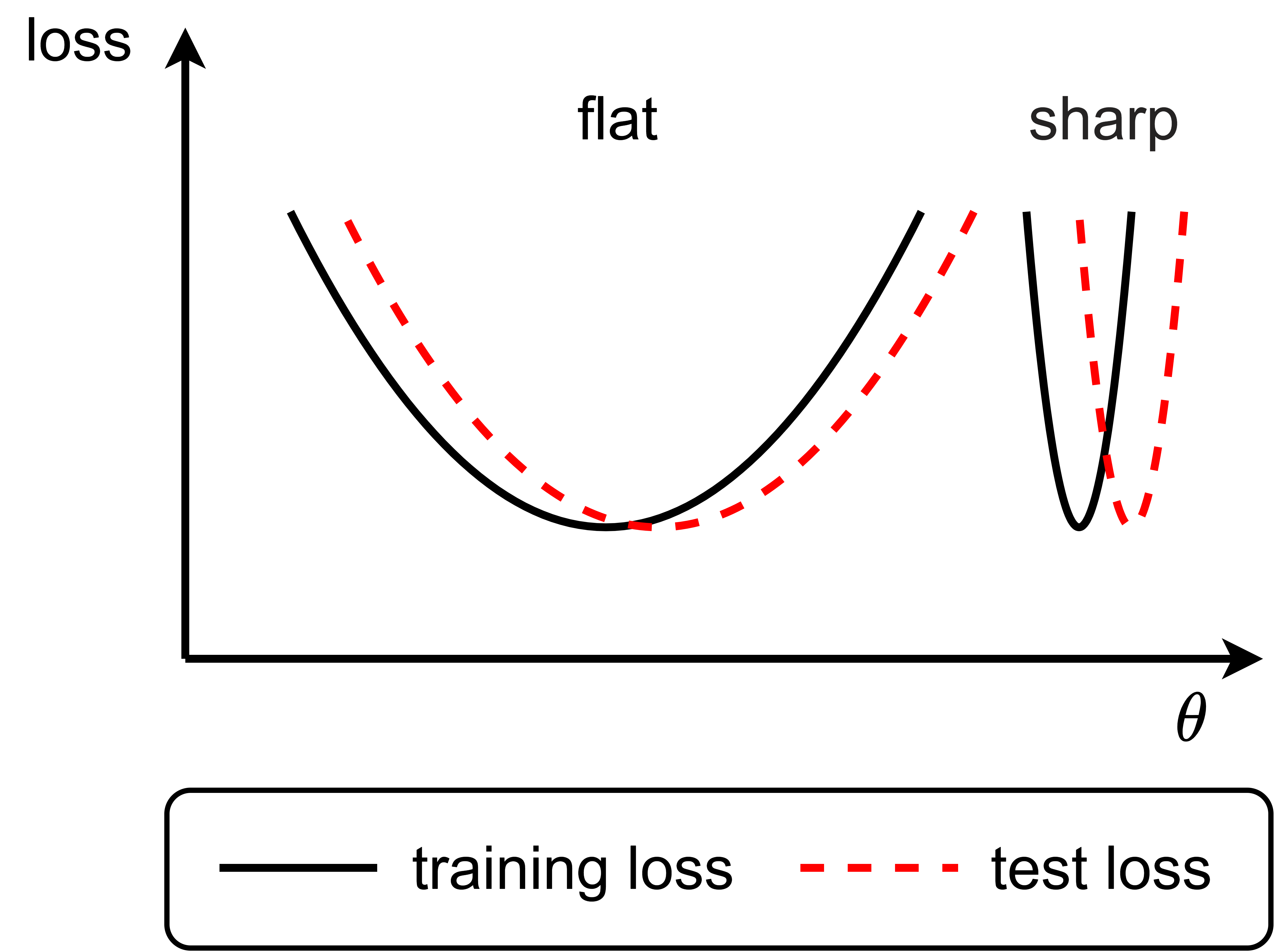
Figure 1: Schematic illustration of an ideal explanation for why flat solutions generalize well (Keskar et al., 2016).

In a neural network training process, one may sometimes observe a phenomenon of loss spike, where the loss rapidly ascends and then descends to the value before the ascent. Typical examples are shown in Fig. 2. We show a special loss landscape structure underlying the loss spike, which is called a smaller-loss-as-sharper (SLAS) structure. In the SLAS structure, the training is driven by descending the loss while entering an increasingly sharp region. Once the sharpness is too large, the loss would ascend exponentially fast. To explain why the loss can descend so fast, we provide a frequency perspective analysis. We find that the deviation in the ascending stage is dominated by low-frequency components. Based on the frequency principle (Xu et al., 2019, 2020) that low-frequency converges faster than high-frequency, we rationalize the fast descent.

The study of loss spike provides an important information that the deviation at the first eigen direction is dominated by low-frequency. We then further argue the link between $\lambda_{\mathrm{max}}$ flatness and generalization. In practical datasets, low-frequency information is often dominant and shared by both the training and the test datasets. Therefore, the training can learn low-frequency well. Since the sharpest direction, indicated by the maximum eigenvalue of the loss Hessian, relates more to the low-frequency, a solution with good generalization and a solution with bad generalization have little difference in the sharpest direction, verified by a series of experiments. Hence, $\lambda_{\mathrm{max}}$ with the intuitive explanation in Fig. 1 encounters difficulty in understanding the generalization of neural networks, such as why a larger learning rate results in better generalization for networks with EoS training.

We also find that a loss spike can facilitate condensation, that is, the input weights of different neurons in the same layer evolve towards the same, which would reduce the network’s effective size. Condensation is a non-linear feature learning phenomenon in neural networks, which may be the underlying mechanism for why the loss spike improves generalization (He et al., 2019; Jastrzebski et al., 2017), rather than simply controlling the value of $\lambda_{\mathrm{max}}$.

This work studies the loss spike from the landscape perspective and the frequency perspective, and revisits the relation between the generalization and the flatness, defined by the maximum eigenvalue of the loss Hessian. This work also conjectures the loss spike may improve generalization via the facilitation of condensation.

2 Related works

Previous works (Cohen et al., 2021; Wu et al., 2018; Xing et al., 2018; Ahn et al., 2022; Lyu et al., 2022; Wang et al., 2022) conduct an extensive study of the EoS phenomenon under various settings. Lewkowycz et al. (2020) observe that when the initial sharpness exceeds $2/\eta$, gradient descent “catapults” into a stable region and converges. Arora et al. (2022) analyze progressive sharpening and the edge of stability phenomenon under specific settings, such as normalized gradient descent. Damian et al. (2022) show that the third-order terms bias towards flatter minima to understand EoS.

Ma et al. (2022) attribute the progressive sharpening to a subquadratic structure of the loss landscape, i.e., the maximum eigenvalue of the loss Hessian is larger when the loss is smaller in a direction. They also propose a flatness-driven motion to study the EoS stage, that is, the training would move towards a flatter minimum, such that the fixed flatness can correspond to points with smaller and smaller loss values due to the subquadratic property. We call this structure a smaller-loss-as-flatter (SLAF) structure. The SLAF structure should expect a continuous decrease in the loss rather than a loss spike. Agarwala et al. (2022) use a quadratic regression model with MSE to study EoS. Similarly, in their model, the loss spike can not happen. Ma et al. (2022) study the loss spike from the perspective of adaptive gradient optimization algorithms, while we focus on the loss landscape structure and use gradient descent training in this paper.

A series of works link the generalization performance of solutions to the landscape of loss functions through the observation that flat minima tend to generalize better (Hochreiter and Schmidhuber, 1997; Wu et al., 2017; Ma and Ying, 2021). Algorithms that favor flat solutions are designed to improve the generalization of the model (Izmailov et al., 2018; Chaudhari et al., 2019; Lin et al., 2018; Zheng et al., 2021; Foret et al., 2020). On the other hand, Dinh et al. (2017) show that sharp minimum can also generalize well by rescaling the parameters at a flat minimum with ReLU activation. In this work, we study the relationship between flatness and generalization from a new perspective, i.e., the frequency perspective, without the limitation of the activation function.

Luo et al. (2021); Zhou et al. (2022) mainly identify the linear regime and the condensed regime of the parameter initialization for two-layer and three-layer wide ReLU NNs, which determines the final fitting result of the network. In the linear regime (Jacot et al., 2018; Arora et al., 2019), the training dynamics of NNs are approximately linear and similar to a random feature model. On the contrary, in the condensed regime, active neurons are condensed at several discrete orientations. At this point, the network is equivalent to another network with a reduced width, which may explain why NNs outperform traditional algorithms (Breiman, 1995; Zhang et al., 2021). For the initial stage of training, A series of works (Zhou et al., 2021; Chen et al., 2023; Maennel et al., 2018; Pellegrini and Biroli, 2020) study the characteristics of the initial condensation for different activation functions. Andriushchenko et al. (2022) find that stochastic gradient descent (SGD) with a large learning rate can facilitate sparse solutions and attributes it to the noise structure of SGD. In our work, we find that for the noise-free full-batch gradient descent algorithm, the loss spike can also facilitate the condensation phenomenon, implying that the noise structure is not the intrinsic cause of condensation.

The frequency principle is examined in extensive datasets and deep neural network models (Xu et al., 2019; Xu and Zhou, 2021; Rahaman et al., 2019). Subsequent theoretical studies show that the frequency principle holds in the general setting with infinite samples (Luo et al., 2021). An overview for frequency principle is referred to Xu et al. (2022). Based on the theoretical understanding, the frequency principle inspires the design of deep neural networks to learn a function with high-frequency fast (Liu et al., 2020; Jagtap et al., 2020; Biland et al., 2019).

3 Preliminary: Linear stability in training quadratic model

We consider a simple quadratic model with the loss $R(\theta)=\lambda\theta^{2}/2$ trained by gradient descent with learning rate $\eta$, $\theta(t+1)=\theta(t)-\eta\cdot dR(\theta)/d\theta$. To ensure the linear stability of the training, it requires $|\theta(t+1)|<|\theta(t)|$, which implies $|1-\lambda\eta|<1$, i.e., otherwise, the training will diverge. Note that $\lambda$ is the Hessian of $R(\theta)$. Similarly, to ensure the linear stability of training a neural network, it requires that the maximum eigenvalue of the loss Hessian is smaller than $2/\eta$, i.e., 2 over the learning rate. Therefore, the maximum eigenvalue of the loss Hessian is often used as the measure of the sharpness of the loss landscape.

4 Loss spike

In this section, we study the phenomenon of loss spike, where the loss would suddenly increase and decrease rapidly. For example, as shown in Fig. 2(a, d), we train a tanh fully-connected neural network (FNN) with 20 hidden neurons for a one-dimensional fitting problem, and a ReLU convolutional neural network (CNN) for the CIFAR10-1k classification problem with MSE. Both two models experience loss spikes. The red curves, i.e., the $\lambda_{\rm max}$ value, show that the loss spikes occur at the EoS stage.

4.1 Typical loss spike experiments

To observe the loss spike clearly, we zoom in on the training epochs around the spike, shown in Fig. 2(b, e). The selected epochs are marked green in Fig. 2(a, d). When the maximum eigenvalue of Hessian $\lambda_{\mathrm{max}}$ (red) exceeds $2/\eta$ (black dashed line), the loss increases, and when $\lambda_{\mathrm{max}}<2/\eta$, the loss decreases, which are consistent with the linear stability analysis.

We then study the parameter space for more detailed characterization. Given $t$ training epochs, and let $\bm{\theta}_{i}$ denote model parameters at epoch $i$, we apply PCA to the matrix $M=[\bm{\theta}_{1}-\bm{\theta}_{t},\cdots,\bm{\theta}_{t}-\bm{\theta}_{t}]$, and then select the first two eigen directions $\bm{e}_{1}$, $\bm{e}_{2}$. The two-dimensional loss surface based on $\bm{e}_{1}$ and $\bm{e}_{2}$ can be calculated by $R_{S}(\bm{\theta}_{t}+\alpha\bm{e}_{1}+\beta\bm{e}_{2})$, where $\alpha$, $\beta$ are the step sizes, and $R_{S}$ is the loss function under the dataset $S$. The trajectory point of parameter $\bm{\theta}_{i}$ can be calculated by the projection of $\bm{\theta}_{i}-\bm{\theta}_{t}$ in the PCA directions, i.e., $(\langle\bm{\theta}_{i}-\bm{\theta}_{t},\bm{e}_{1}\rangle,\langle\bm{\theta}_{i}-\bm{\theta}_{t},\bm{e}_{2}\rangle)$. Parameter trajectories (blue dots) and loss surfaces along PCA directions are shown in Fig. 2(c, f). In two distinct examples, they exhibit similar behaviors. At the beginning of the ascent stage of the spike, the parameter is at a small-loss region, where the opening of the contour lines is towards the left, indicating a leftward component of descent direction. In the left region, the contour lines are denser, implying a sharper loss surface. Once $\lambda_{\rm max}>2/\eta$, the parameters become unstable, and the loss value increases exponentially. In the large-loss region, the opening of the contour shifts to the right, indicating a rightward component of the descent direction, resulting in a sparser contour, i.e., a flatter loss surface. After several steps, when $\lambda_{\rm max}<2/\eta$, the training returns to the stable stage.

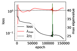
(a) FNN, full loss

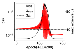
(b) FNN, loss

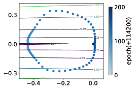
(c) FNN, trajectory

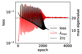
(d) CNN, full loss

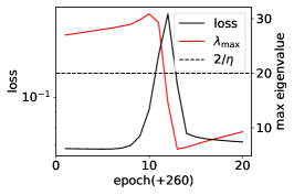
(e) CNN, loss

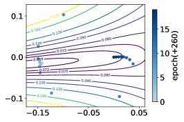
(f) CNN, trajectory

Figure 2: (a, d) The loss value (black) and $\lambda_{\rm max}$ (red) vs. training epoch, where the $\lambda_{\rm max}$ is calculated every 100 epoch. (b, e) The loss value and $\lambda_{\rm max}$ of a specific epoch interval, which is marked green in (a, d), respectively. (c, f) The loss surface and the trajectory of the model parameters along the first two PCA directions. (a, b, c) Two-layer tanh NN with width 20. The sum of the explained variance ratios of the first two PCA directions is 0.9895. (d, e, f) Two-layer ReLU CNN with Max Pooling. The sum of the explained variance ratios of the first two PCA directions is 0.9882.

4.2 Smaller-loss-as-sharper (SLAS) structure

The above experiments reveal a common structure that causes a loss spike, namely, the $\lambda_{\mathrm{max}}$ sharpness increases in the direction of decreasing loss. We call this structure smaller-loss-as-sharper (SLAS) structure. The SLAS structure differs from the SLAF (smaller-loss-as-flatter) structure studied in Ma et al. (2022), which is also common in the EoS stage as shown in Fig. 3(a). A toy example of the SLAS structure is shown in Fig. 3(b). The left cross-section of the loss landscape has a flatter curvature while the right one has a sharper curvature. At the minimum of the left cross-section (the $L_{1}$ dashed line), the opening of the contour lines towards the right and the parameter point will also move right, which makes the curvature sharper. Once $\eta>2/\lambda_{\rm max}$, it starts to diverge to a large-loss region and the opening of the contour turns left (the $L_{2}$ dashed line), which makes the curvature flatter.

The following quadratic model is a simple example of SLAS structure,

$$f(x,y)=(50x+200)y^{2}-x+5,$$ (1)

where $(x,y)\in(-4,+\infty)\times\mathbb{R}$. For any constant $C$, $y=0$ is the minimum point of $f(C,y)$, and the larger $x$ is, the sharper the loss landscape in the $y$-direction. As shown in Fig. 3(c, d), the loss curve and the trajectory of parameters are similar to the realistic example above, where the parameters move toward the sharp direction at the beginning of the loss spike, and then move toward the flat direction. The intuitive explanation for the above phenomenon is that as $x$ increases, $f(x,0)$ decreases, which means that $f(x,0)$ has a smaller value at the sharp region, i.e., the SLAS structure, which makes the opening of the contour lines towards different directions at different loss levels.

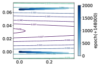
(a) SLAF example

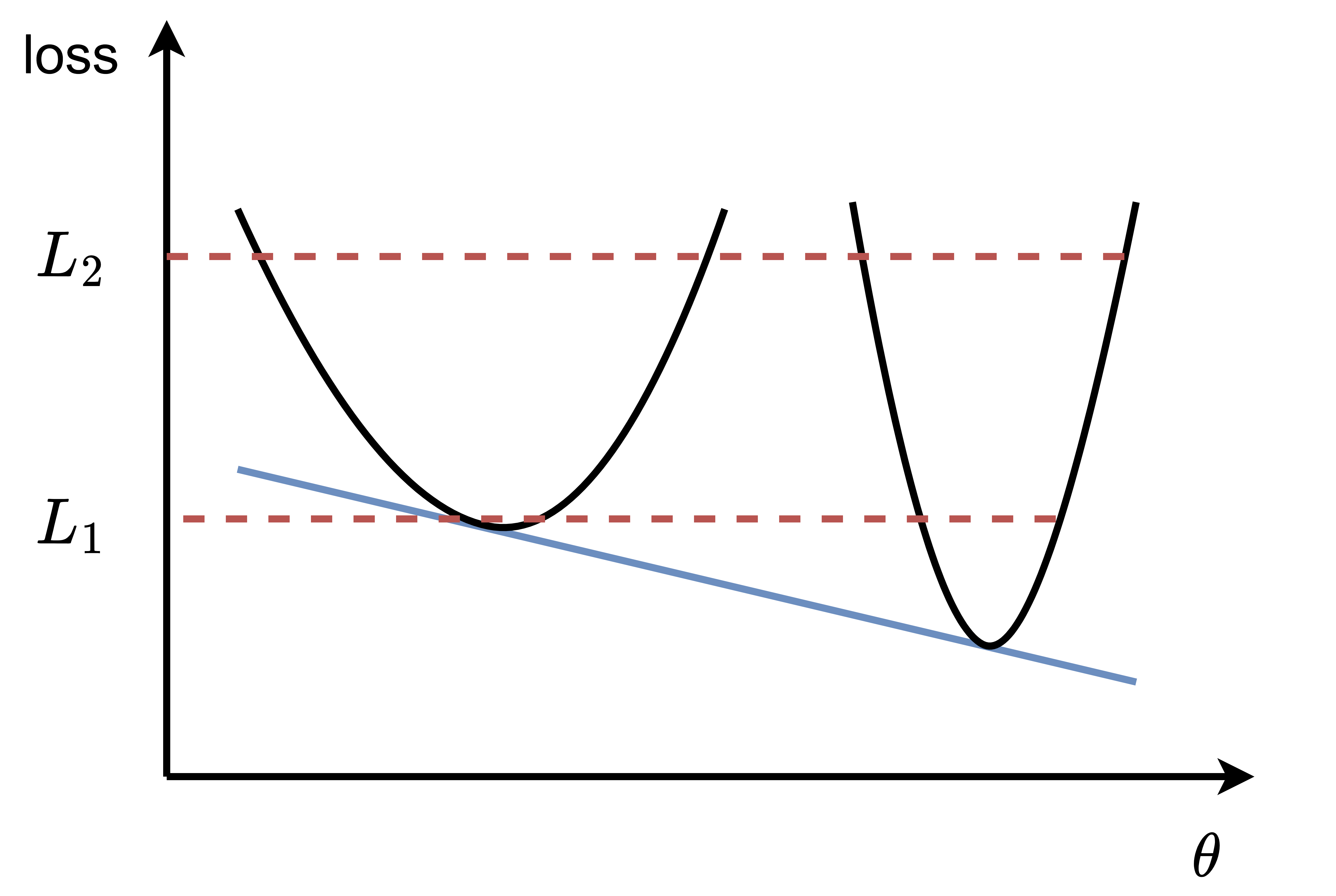
(b) schematic illustration

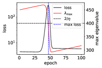
(c) toy model, loss

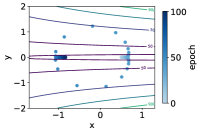
(d) toy model, trajectory

Figure 3: (a) The loss surface and the trajectory of the model parameters along the first two PCA directions in the EoS stage. (b) Schematic illustration of SLAS structure. (c) The loss value and the maximum eigenvalue of the Hessian matrix of a loss spike process of the toy model. (d) The loss surface and the GD trajectory of the two-dimensional parameters of the toy model.

For this example, we can exactly compute the derivative of Eq. (1) as follows:

$$\frac{\partial f(x,y)}{\partial x}=50y^{2}-1.$$

Thus we have

$$\frac{\partial f(x,y)}{\partial x}\begin{cases}>0&\text{ if }f(x,y)<9\\ =0&\text{ if }f(x,y)=9\\ <0&\text{ if }f(x,y)>9\end{cases},$$

which indicates that the toy model has a positive gradient component in the $x$ direction when the parameters are in the small-loss region ($f(x,y)<9$), while a negative gradient component in the $x$ direction when the parameters are in the large-loss region ($f(x,y)>9$).

Although the SLAS structure can explain the mechanism of the ascent stage based on the toy model, it can not explain the reason for the rapid descent of the loss in the descent phase of the loss spike, which takes much fewer steps than the training from the same level loss at the initialization. For instance, for the quadratic model in the Preliminary section, the descent would be very slow if the learning rate is slightly smaller than $2/\lambda_{\mathrm{max}}$. Moreover, due to the high dimensionality of the parameter space, the parameter trajectory does not always align with the first eigen direction, otherwise, as shown in the toy model, the loss would not decrease continuously. In the following, we take a step toward understanding the rapid decrease from the frequency perspective.

4.3 Frequency perspective for understanding descent stage

In this subsection, we study the mechanism of the rapid loss descent during the descent stage in a loss spike from the perspective of frequency.

We base our analysis on a common phenomenon of frequency principle (Xu et al., 2019, 2020; Zhang et al., 2021; Luo et al., 2021; Rahaman et al., 2019; Ronen et al., 2019), which states that deep NNs often fit target functions from low to high frequencies during the training. A series of frequency principle works show that low-frequency can converge faster than high-frequency. Compared to the peak point of the loss spike with the point with the same loss value at the initial training, the descent during the spike should eliminate more low-frequency with a fast speed while the descent from the initial model should eliminate more high-frequency with a slow speed. To verify this conjecture, we study the frequency distribution of the converged part during the descent stage.

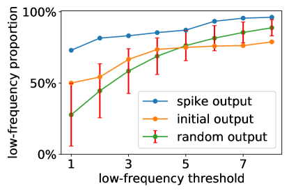
Figure 4: Low-frequency proportion for different low-frequency thresholds. The NN we used is a two-layer tanh NN with width 20. For the random output difference, we calculate the mean value and the error bar with 100 random samples.

The peak of the loss spike is denoted as $\bm{\theta}_{\mathrm{max}}$, the initial point which has the similar loss of $\bm{\theta}_{\mathrm{max}}$ is denoted as $\bm{\theta}_{\mathrm{ini,m}}$, the parameter at the end of the loss spike (a point is roughly selected when the descent is slow) is denoted as $\bm{\theta}_{\mathrm{end}}$. We then study the frequency distribution of spike output difference $f_{\rm peak,diff}:=f_{\bm{\theta}_{\mathrm{max}}}-f_{\bm{\theta}_{\mathrm{end}}}$ and initial output difference $f_{\rm ini,diff}:=f_{\bm{\theta}_{\mathrm{ini,m}}}-f_{\bm{\theta}_{\mathrm{end}}}$.

For comparison, we also randomly select parameter $\bm{\theta}_{\mathrm{rnd}}:=\bm{\theta}_{\mathrm{end}}+(\lVert\bm{\theta}_{\mathrm{end}}-\bm{\theta}_{\mathrm{max}}\rVert_{2}/\lVert\varepsilon\rVert_{2})\varepsilon$, where $\varepsilon\sim N(0,I)$ is a random variable. We then study the frequency distribution of random output difference $f_{\rm rnd,diff}:=f_{\bm{\theta}_{\mathrm{rnd}}}-f_{\bm{\theta}_{\mathrm{end}}}$.

We characterize the frequency distribution by taking different low-frequency thresholds to study low-frequency proportion. For a low-frequency threshold $K$, a low-frequency proportion (LFP) is defined as follows to characterize the power proportion of the low-frequency component over the whole spectrum,

$$\mathrm{LFP}(K)=\frac{\sum_{k\leq K}\lVert\hat{f}_{\bm{\theta}}(k)\rVert^{2}}{\sum_{k}\lVert\hat{f}_{\bm{\theta}}(k)\rVert^{2}},$$ (2)

where $\hat{f}_{\bm{\theta}}$ indicates the Fourier transform of function $f_{\bm{\theta}}$.

As shown in Fig. 4, the low-frequency proportion of the spike output difference is significantly larger than the low-frequency proportion of the initial output difference and the random output difference, where we take 100 samples of random variable $\varepsilon$ for the mean value and the error bar for each low-frequency threshold. The large low-frequency proportion of the spike output difference is the key reason for the rapid drop in the loss value during the descent stage, as suggested by the frequency principle.

5 Revisit the flatness-generalization picture

Motivated by the loss spike analysis from the frequency perspective, we further revisit the common flatness-generalization picture. A series of previous works (Hochreiter and Schmidhuber, 1997; Li et al., 2017) attempt to link the flatness of the loss landscape with generalization, so as to characterize the model through flatness conveniently. A classic empirical illustration is shown in Fig. 1, which vividly expresses the reason why flat solutions tend to have better generalization. Usually, the training loss landscape and the test landscape do not exactly coincide due to sampling noise. A flat solution would be robust to the perturbation while a sharp solution would not. For such a one-dimensional case, this analysis is valid, but the loss landscape of a NN case is very high-dimensional, and such simple visualization or explanation is yet to be validated.

The first eigen direction of the loss Hessian, i.e., the eigen direction corresponding to the maximum eigenvalue, is the sharpest direction. Based on the flatness-generalization picture, it is natural to use the maximum eigenvalue as the measure for the flatness, which can also indicate generalization. However, this naive analysis is not always correct for neural networks.

5.1 Frequency perspective

Since the maximum eigenvalue of the loss Hessian can indicate the linear stability of the training, it is often used as a measure for flatness/sharpness, that is, a larger maximum eigenvalue indicates a sharper loss landscape. As shown by the linear stability analysis, once the maximum eigenvalue is larger than $2/\eta$, the training would oscillate and diverge along the first eigen direction. Meanwhile, as the parameter moves away from the minimum point along the first eigen direction, the loss spike is mainly due to the large low-frequency difference as shown in Fig. 4. Therefore, the deviation in the first eigen direction of the loss Hessian mainly leads to the deviation of low-frequency components.

In order to examine the above analysis, we first obtain the model parameter $\bm{\theta}_{\rm train}$ with poor generalization by training the model initialized in the linear regime (Luo et al., 2021), and then further train the model parameter $\bm{\theta}_{\rm train}$ on the test dataset with a small learning rate to obtain the model parameter $\bm{\theta}_{\rm test}$.

We study the impact of each eigen direction on the test loss by eliminating the difference between $\bm{\theta}_{\rm train}$ and $\bm{\theta}_{\rm test}$ in the $i$-th eigen direction $\bm{\nu}_{i}$, where $i$ is the index of eigenvalues. As shown in Fig. 5(a), we study the change of the test loss $L(i)$ with the eigenvalue index $i$ as follows to study the effect of eigenvectors on generalization,

$$L(i)=R_{S_{\rm test}}\left(\bm{\theta}_{\rm train}+\sum_{j=1}^{i}\langle\bm{\theta}_{\rm test}-\bm{\theta}_{\rm train},\bm{\nu}_{j}\rangle\bm{\nu}_{j}\right),$$

where $S_{\rm test}$ is the test dataset. The movement of parameters on the eigenvectors corresponding to large eigenvalues has a weak impact on the test loss, while the movement of parameters on the eigenvectors corresponding to small eigenvalues has a significant impact on the test loss.

A reasonable explanation from the perspective of frequency is as follows. In common datasets, low-frequency components often dominate over high-frequency ones. For noisy sampling, the dominant low-frequency is shared by both the training and the test data. When the parameters move along the eigen directions corresponding to the large eigenvalues, the network output often changes at low-frequency, which is already captured by both $\bm{\theta}_{\rm train}$ and $\bm{\theta}_{\rm test}$. Therefore, the improvement of model generalization often requires certain high-frequency changes. As shown in Fig. 5(b), we move the corresponding $\bm{\theta}_{\rm train}$ along the first nine eigen directions, and show the difference between the network outputs before and after the movement, i.e., $f_{\bm{\theta}_{{\rm train}+\bm{\nu}_{i}/\sqrt{\lambda_{i}}}}-f_{\bm{\theta}_{\rm train}}$, where the $1/\sqrt{\lambda_{i}}$ item is to make the loss of the network moved in different eigen directions approximately the same. From the difference between the outputs before and after the movement, it can be seen that when the parameters move along the eigen direction corresponding to the larger eigenvalue, the change of the model output is often less oscillated, i.e., dominated by the lower-frequency. Since the low-frequency is captured by both $\bm{\theta}_{\rm train}$ and $\bm{\theta}_{\rm test}$, they should be close in the eigen directions corresponding to large eigenvalues, which is verified in the following subsection.

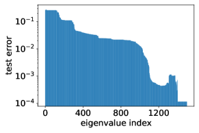
(a) FNN

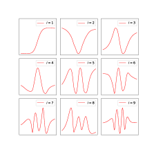
(b) output difference

Figure 5: Two-layer tanh FNN with a width of 500. (a) The variation of the test loss with the eigenvalue index $i$ when eliminating the difference between $\bm{\theta}_{\rm train}$ and $\bm{\theta}_{\rm test}$ in the first $i$ eigen directions. (b) The output difference before and after moving $\theta_{\rm train}$ in the first nine eigen directions of its Hessian matrix. Each subset corresponds to the case of one eigen direction.

5.2 Difference on each eigen direction

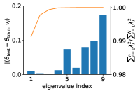
(a) FNN

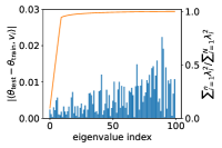
(b) Two-layer CNN

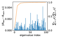
(c) Three-layer CNN

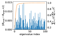
(d) Different batch sizes

Figure 6: Blue bar: (a, b, c) show the projection values of in each eigen direction of $H(\bm{\theta}_{\rm train})$ for $\bm{\theta}_{\rm test}-\bm{\theta}_{\rm train}$, and (d) for $\bm{\theta}_{\mathrm{large}}-\bm{\theta}_{\mathrm{small}}$. Orange line: the sum of the first $n$ eigenvalues over all eigenvalues. (a) Two-layer tanh FNN for the one-dimensional fitting problem. (b) Two-layer ReLU CNN with Max Pooling for the CIFAR10 classification problem. (c) Three-layer ReLU CNN with Max Pooling for the CIFAR10 classification problem. (d) Five-layer ReLU CNN with Max Pooling for the CIFAR10 classification problem.

We then examine the projection of $\bm{\theta}_{\rm test}-\bm{\theta}_{\rm train}$ in each eigen direction of $H(\bm{\theta}_{\rm train})$. As shown in Fig. 6, we show the projection of $\bm{\theta}_{\rm test}-\bm{\theta}_{\rm train}$ on each eigenvector $\bm{\nu}_{i}$ (blue bar) for the FNN on function fitting problem and the CNNs on CIFAR10 classification problem. Due to the high complexity of calculating the eigenvectors of the large-size Hessian matrix, we use the Lanczos method (Cullum and Willoughby, 2002) to numerically compute the first $N$ eigenvalues and their corresponding eigenvectors. For $n<N$, we use ${\sum}_{i=1}^{n}\lambda_{i}^{2}/{\sum}_{i=1}^{N}\lambda_{i}^{2}$ to represent the explained variance ratio, i.e., to measure how much flatness information the first $n$ eigen directions (orange line) can explain. For different network structures and model tasks, the projection value of $\bm{\theta}_{\rm test}-\bm{\theta}_{\rm train}$ on the eigenvector $\bm{\nu}_{i}$ has a positive correlation with the eigenvalue index $i$, which confirms that $\bm{\theta}_{\rm train}$ and $\bm{\theta}_{\rm test}$ have little difference on low-frequency part. Note that in Fig. 6(d), the two minima, $\bm{\theta}_{\mathrm{small}}$ and $\bm{\theta}_{\mathrm{large}}$, are found by small and large batch sizes, respectively, and they also have little difference in eigen directions corresponding to large eigenvalues.

5.3 Implications

The above analysis suggests the following implications: i) The maximum eigenvalue of the loss Hessian is a good measure of sharpness for whether the training is linearly stable but not a good measure for generalization; ii) The common low-dimensional flatness-generalization picture suffers difficulty in understanding the high-dimensional loss landscape of neural network. The generalization performance is a combined effect of most eigen directions, including those with small eigenvalues.

6 Loss spike facilitates condensation

From the analysis above, the restriction on $\lambda_{\rm max}$ does not seem to be the essential reason why loss spike affects the generalization of the model. In this section, we study the effect of loss spike on condensation, which may improve the model’s generalization in some situations (He et al., 2019; Jastrzebski et al., 2017). A condensed network, which refers to a network with neurons condensing in several discrete directions, is equivalent to another smaller network (Zhou et al., 2021; Luo et al., 2021). It has a lower effective complexity than it appears. The embedding principle (Zhang et al., 2021, 2022; Fukumizu et al., 2019; Simsek et al., 2021) shows that a condensed network, although equivalent to a smaller one in approximation, has more degeneracy and descent directions that may accelerate the training process. The low effective complexity and simple training process may be underlying reasons for good generalization. We show that the loss spike can facilitate the condensation phenomenon for the noise-free full-batch gradient descent algorithm.

As shown in Fig. 7, we train a tanh NN with 100 hidden neurons for the one-dimensional fitting problem to fit the data using MSE as the loss function. Additional experimental verification on ReLU NNs is provided in Appendix B.1. To clearly study the effect of loss spike on condensation, we take the parameter initialization distribution in the linear regime (Luo et al., 2021) that does not induce condensation without additional constraints. For NNs with identical initialization, we train the network separately with a small learning rate (blue) and a large learning rate (orange). For the left subfigure in Fig. 7, the loss value has a significant spike for the large learning rate, but not for the small one. At the same time, the middle subfigure reveals that the model output without a loss spike (blue) during the training process has more oscillation than the model output with a loss spike (orange). We study the features of parameters to understand the underlying effect of loss spike better.

To study the parameter features, we measure each parameter pair $(a_{j},\bm{w}_{j})$ by the feature direction $\hat{\bm{w}}_{j}=\bm{w}_{j}/\lVert\bm{w}_{j}\rVert_{2}$ and amplitude $A_{j}=|a_{j}|\lVert\bm{w}_{j}\rVert_{2}$. For a NN with one-dimensional input, after incorporating the bias term, $\bm{w}_{j}$ is two-dimensional, and we use the angle between $\bm{w}_{j}$ and the unit vector $(1,0)$ to indicate the orientation of each neuron. The scatter plots of $\{(\hat{\bm{w}}_{j},|a_{j}|)\}_{j=1}^{m}$ and $\{(\hat{\bm{w}}_{j},\lVert\bm{w}_{j}\rVert_{2})\}_{j=1}^{m}$ of tanh activation are presented in Appendix B to eliminate the impact of the non-homogeneity of tanh activation.

The scatter plots of $\{(\hat{\bm{w}}_{j},A_{j})\}_{j=1}^{m}$ of the NN is shown in the right subfigure of Fig. 7. Parameters without loss spikes (blue) are closer to the initial values (green) than those with loss spikes (orange). For the case with loss spikes, non-zero parameters tend to condense in several discrete orientations, showing a tendency to condensation.

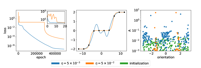
Figure 7: Comparison of two-layer tanh NNs with identical initialization but different learning rates $\eta$. The loss spike occurs at a large learning rate (orange), while not at a small learning rate (blue). Left: loss vs. epoch. The small picture in the upper right corner shows the occurrence of the loss spike in more detail. Middle: output. Right: The weight feature distribution of the trained models and the initial one.

7 Conclusion and discussion

In this work, we provide an explanation for loss spikes in neural network training. We explain the ascent stage based on the landscape structure, i.e., the SLAS structure, and for the descent stage, we explain it from the perspective of frequency. We revisit the common flatness-generalization picture based on the frequency analysis. We also find that noise-free gradient descent with loss spikes can facilitate condensation, which may be an underlying reason for the good generalization in some situations. Obviously, many questions remain open. For example, why the eigen direction corresponding to a large eigenvalue is dominated by low-frequency? Why the loss spike can facilitate the condensation? We leave the discussion of these important questions to future work.

Appendix A Experimental setups

For Fig. 2(a-c), Fig. 3(a), Fig. 4, we use the two-layer tanh FNN with a width of 20 to fit the target function using full-batch gradient descent as follows,

$$f(x)=\mathrm{sin}(x)+\mathrm{sin}(4x).$$

The initialization of the parameters $\bm{\theta}\sim N(0,m^{-1})$, where $m$ is the width of the NN, and the learning rate $\eta=0.05$. For Fig. 2(a), the $\lambda_{\rm max}$ is calculated every 100 epochs. Fig. 2(c) and Fig. 3(a) show the parameter trajectories of different epoch intervals, which are indicated on the label of the color bar. For Fig. 4, the $\bm{\theta}_{\rm max}$ is selected at epoch 114320, and the $\bm{\theta}_{\rm end}$ is selected at epoch 114400.

For Fig. 2(d-f), we use the two-layer ReLU CNN with a Max Pooling layer behind the activation function for the CIFAR10-1k classification problem, i.e., using the first 1000 training data of the CIFAR10 as the training data. The number of the convolution kernels is 16 and the size is $3\times 3$. We use the MSE as the loss function with learning rate $\eta=0.1$.

For Fig. 3, we use the following quadratic model as the toy model to illustrate the SLAS structure,

$$f(x,y)=(50x+200)y^{2}-x+5,$$

where $(x,y)\in(-4,+\infty)\times\mathbb{R}$. The training uses the gradient descent algorithm with learning rate $\eta=5\times 10^{-3}$ and the initial value $(x,y)=(0.5,0.00001)$.

For Fig. 5(a, b) and Fig. 6(a), we use the two-layer tanh FNN with a width of 500 to fit the target function using full-batch gradient descent as follows,

$$f(x)=\mathrm{tanh}(x-6)+\mathrm{tanh}(x+6).$$

The initialization of the parameters $\bm{\theta}\sim N(0,m^{-0.4})$, where $m$ is the width of the NN, and the learning rate $\eta=0.001$. The training dataset is obtained by sampling 15 points equidistantly in the $[-12,12]$ interval, and the test dataset is obtained by sampling 14 points equidistantly in the $[-11.14,11.14]$ interval, which is approximately the midpoint of the pairwise data of the training set.

For Fig. 6(b-c), we use the CNNs for the CIFAR10-1k classification problem with structures shown in Table 1-2, respectively. We use ReLU as the activation function, added behind each convolutional layer. We use the Xavier initialization and the MSE loss function. The learning rate is 0.005. For Fig. 6(d), we use the CNNs for the CIFAR10-2k classification problem with structures shown in Table 3. We use ReLU as the activation function, added behind each convolutional layer. We use the Xavier initialization and the cross-entropy loss function. The learning rate is 0.01. The large batch size we used is 1000, while the small one is 32.

Table 1: The architecture of the three-layer CNN used in Fig. 6(b).

Layer	Output size
input	$32\times 32\times 3$
$3\times 3\times 16$, conv	$32\times 32\times 16$
$2\times 2$, maxpool	$16\times 16\times 16$
flatten	$4096$
$4096\rightarrow 10$, linear	10

Table 2: The architecture of the three-layer CNN used in Fig. 6(c).

Layer	Output size
input	$32\times 32\times 3$
$3\times 3\times 16$, conv	$32\times 32\times 16$
$2\times 2$, maxpool	$16\times 16\times 16$
$3\times 3\times 32$, conv	$16\times 16\times 32$
$2\times 2$, maxpool	$8\times 8\times 32$
flatten	$2048$
$2048\rightarrow 10$, linear	10

Table 3: The architecture of the five-layer CNN used in Fig. 6(d).

Layer	Output size
input	$32\times 32\times 3$
$3\times 3\times 16$, conv	$32\times 32\times 16$
$2\times 2$, maxpool	$16\times 16\times 16$
$3\times 3\times 32$, conv	$16\times 16\times 32$
$2\times 2$, maxpool	$8\times 8\times 32$
$3\times 3\times 64$, conv	$8\times 8\times 64$
$2\times 2$, maxpool	$4\times 4\times 64$
flatten	$1024$
$2048\rightarrow 500$, linear	500
$500\rightarrow 10$, linear	10

For Fig. 7, Fig. 9, we use the two-layer tanh FNN with a width of 200 to fit the target function using full-batch gradient descent as follows,

$$f(x)=\mathrm{tanh}(x-6)+\mathrm{tanh}(x+6).$$

The initialization of the parameters $\bm{\theta}\sim N(0,m^{-1})$, where $m$ is the width of the NN. We train the NN with loss spikes using the learning rate $\eta=0.05$ while using $\eta=0.005$ for the training without loss spikes. The training dataset is obtained by sampling 10 points equidistantly in the $[-12,12]$ interval.

For Fig. 8, we use the two-layer ReLU FNN with a width of 500 to fit the target function using full-batch gradient descent as follows,

$$f(x)=\frac{1}{2}\mathrm{ReLU}(-x-\frac{1}{3})+\frac{1}{2}\mathrm{ReLU}(x-\frac{1}{3}).$$

The initialization of the parameters $\bm{\theta}\sim N(0,m^{-0.4})$, where $m$ is the width of the NN. We train the NN with loss spikes using the learning rate $\eta=0.05$ while using $\eta=0.0005$ for the training without loss spikes. The training dataset is obtained by sampling 6 points equidistantly in the $[-5/3,5/3]$ interval.

Appendix B Experimental results

B.1 Loss spikes facilitate condensation on ReLU NNs

In this subsection, We verify that the ReLU network facilitates condensation with loss spikes shown in Fig. 8, similar to the situation in the tanh NNs shown in Fig. 7 in the main text. We only plot the neurons with non-zero output value in the data interval $[x_{1},x_{n}]$ in the situation in the ReLU NNs. For the neurons with constant zero output value in the data interval, they will not affect the training process and the NN’s output.

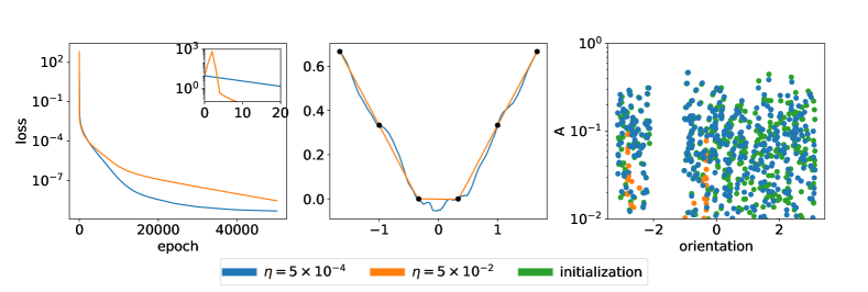
Figure 8: Comparison of two-layer ReLU NNs with the same initialization at different learning rates $\eta$. The loss spike occurs at a large learning rate, while does not occur at a small learning rate. Left: The loss value under different learning rates, $\eta=5\times 10^{-4}$ (blue) and $\eta=5\times 10^{-2}$ (orange). The small picture in the upper right corner shows the occurrence of the loss spike in more detail. Middle: The output of the model trained under different learning rates, $\eta=5\times 10^{-4}$ (blue) and $\eta=5\times 10^{-2}$ (orange). The black points are the target points. Right: The feature of the model trained under different learning rates, $\eta=5\times 10^{-4}$ (blue) and $\eta=5\times 10^{-2}$ (orange) and the initialization (green).

B.2 Detailed Features of Tanh NNs

In order to eliminate the influence of the inhomogeneity of the tanh activation function on the parameter features of Fig. 7, we plot the normalized scatter figures between $\lVert a_{j}\rVert$, $\lVert\bm{w}_{j}\rVert$ and the orientation, as shown in Fig. 9. Obviously, for the network with loss spikes, both the input weight and the output weight have weight condensation, while the network without loss spikes does not have weight condensation.

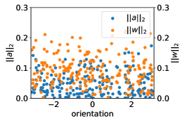
(a) initialization

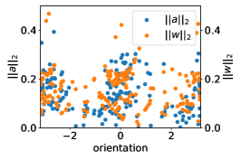
(b) $\eta=5\times 10^{-3}$

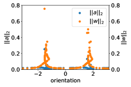
(c) $\eta=5\times 10^{-2}$

Figure 9: The normalized scatter diagrams between $\lVert a_{j}\rVert$, $\lVert\bm{w}_{j}\rVert$ and the orientation of tanh NNs for the initialization parameters and the parameters trained with and without loss spikes. Blue dots and orange dots are the output weight distribution and the input weight distribution, respectively.

References

- Wu et al. (2018) L. Wu, C. Ma, W. E, How sgd selects the global minima in over-parameterized learning: A dynamical stability perspective, Advances in Neural Information Processing Systems 31 (2018).
- Cohen et al. (2021) J. M. Cohen, S. Kaur, Y. Li, J. Z. Kolter, A. Talwalkar, Gradient descent on neural networks typically occurs at the edge of stability, arXiv preprint arXiv:2103.00065 (2021).
- Arora et al. (2022) S. Arora, Z. Li, A. Panigrahi, Understanding gradient descent on the edge of stability in deep learning, in: International Conference on Machine Learning, PMLR, 2022, pp. 948–1024.
- Keskar et al. (2016) N. S. Keskar, D. Mudigere, J. Nocedal, M. Smelyanskiy, P. T. P. Tang, On large-batch training for deep learning: Generalization gap and sharp minima, arXiv preprint arXiv:1609.04836 (2016).
- Hochreiter and Schmidhuber (1997) S. Hochreiter, J. Schmidhuber, Flat minima, Neural computation 9 (1997) 1–42.
- Xu et al. (2019) Z.-Q. J. Xu, Y. Zhang, Y. Xiao, Training behavior of deep neural network in frequency domain, in: International Conference on Neural Information Processing, Springer, 2019, pp. 264–274.
- Xu et al. (2020) Z.-Q. J. Xu, Y. Zhang, T. Luo, Y. Xiao, Z. Ma, Frequency principle: Fourier analysis sheds light on deep neural networks, Communications in Computational Physics 28 (2020) 1746–1767.
- He et al. (2019) F. He, T. Liu, D. Tao, Control batch size and learning rate to generalize well: Theoretical and empirical evidence, Advances in Neural Information Processing Systems 32 (2019).
- Jastrzebski et al. (2017) S. Jastrzebski, Z. Kenton, D. Arpit, N. Ballas, A. Fischer, Y. Bengio, A. Storkey, Three factors influencing minima in sgd, arXiv preprint arXiv:1711.04623 (2017).
- Xing et al. (2018) C. Xing, D. Arpit, C. Tsirigotis, Y. Bengio, A walk with sgd, arXiv preprint arXiv:1802.08770 (2018).
- Ahn et al. (2022) K. Ahn, J. Zhang, S. Sra, Understanding the unstable convergence of gradient descent, in: International Conference on Machine Learning, PMLR, 2022, pp. 247–257.
- Lyu et al. (2022) K. Lyu, Z. Li, S. Arora, Understanding the generalization benefit of normalization layers: Sharpness reduction, arXiv preprint arXiv:2206.07085 (2022).
- Wang et al. (2022) Z. Wang, Z. Li, J. Li, Analyzing sharpness along gd trajectory: Progressive sharpening and edge of stability, Advances in Neural Information Processing Systems 35 (2022) 9983–9994.
- Lewkowycz et al. (2020) A. Lewkowycz, Y. Bahri, E. Dyer, J. Sohl-Dickstein, G. Gur-Ari, The large learning rate phase of deep learning: the catapult mechanism, arXiv preprint arXiv:2003.02218 (2020).
- Damian et al. (2022) A. Damian, E. Nichani, J. D. Lee, Self-stabilization: The implicit bias of gradient descent at the edge of stability, arXiv preprint arXiv:2209.15594 (2022).
- Ma et al. (2022) C. Ma, D. Kunin, L. Wu, L. Ying, Beyond the quadratic approximation: The multiscale structure of neural network loss landscapes, Journal of Machine Learning 1 (2022) 247–267. URL: http://global-sci.org/intro/article_detail/jml/21028.html. doi:https://doi.org/10.4208/jml.220404.
- Agarwala et al. (2022) A. Agarwala, F. Pedregosa, J. Pennington, Second-order regression models exhibit progressive sharpening to the edge of stability, arXiv preprint arXiv:2210.04860 (2022).
- Ma et al. (2022) C. Ma, L. Wu, E. Weinan, A qualitative study of the dynamic behavior for adaptive gradient algorithms, in: Mathematical and Scientific Machine Learning, PMLR, 2022, pp. 671–692.
- Wu et al. (2017) L. Wu, Z. Zhu, et al., Towards understanding generalization of deep learning: Perspective of loss landscapes, arXiv preprint arXiv:1706.10239 (2017).
- Ma and Ying (2021) C. Ma, L. Ying, On linear stability of sgd and input-smoothness of neural networks, Advances in Neural Information Processing Systems 34 (2021) 16805–16817.
- Izmailov et al. (2018) P. Izmailov, A. Wilson, D. Podoprikhin, D. Vetrov, T. Garipov, Averaging weights leads to wider optima and better generalization, in: 34th Conference on Uncertainty in Artificial Intelligence 2018, UAI 2018, 2018, pp. 876–885.
- Chaudhari et al. (2019) P. Chaudhari, A. Choromanska, S. Soatto, Y. LeCun, C. Baldassi, C. Borgs, J. Chayes, L. Sagun, R. Zecchina, Entropy-sgd: Biasing gradient descent into wide valleys, Journal of Statistical Mechanics: Theory and Experiment 2019 (2019) 124018.
- Lin et al. (2018) T. Lin, S. U. Stich, K. K. Patel, M. Jaggi, Don’t use large mini-batches, use local sgd, arXiv preprint arXiv:1808.07217 (2018).
- Zheng et al. (2021) Y. Zheng, R. Zhang, Y. Mao, Regularizing neural networks via adversarial model perturbation, in: Proceedings of the IEEE/CVF Conference on Computer Vision and Pattern Recognition, 2021, pp. 8156–8165.
- Foret et al. (2020) P. Foret, A. Kleiner, H. Mobahi, B. Neyshabur, Sharpness-aware minimization for efficiently improving generalization, arXiv preprint arXiv:2010.01412 (2020).
- Dinh et al. (2017) L. Dinh, R. Pascanu, S. Bengio, Y. Bengio, Sharp minima can generalize for deep nets, in: International Conference on Machine Learning, PMLR, 2017, pp. 1019–1028.
- Luo et al. (2021) T. Luo, Z.-Q. J. Xu, Z. Ma, Y. Zhang, Phase diagram for two-layer relu neural networks at infinite-width limit, Journal of Machine Learning Research 22 (2021) 1–47.
- Zhou et al. (2022) H. Zhou, Q. Zhou, Z. Jin, T. Luo, Y. Zhang, Z.-Q. J. Xu, Empirical phase diagram for three-layer neural networks with infinite width, Advances in Neural Information Processing Systems (2022).
- Jacot et al. (2018) A. Jacot, C. Hongler, F. Gabriel, Neural tangent kernel: Convergence and generalization in neural networks, in: Advances in Neural Information Processing Systems, 2018, pp. 8580–8589.
- Arora et al. (2019) S. Arora, S. S. Du, W. Hu, Z. Li, R. R. Salakhutdinov, R. Wang, On exact computation with an infinitely wide neural net, Advances in neural information processing systems 32 (2019).
- Breiman (1995) L. Breiman, Reflections after refereeing papers for nips, The Mathematics of Generalization XX (1995) 11–15.
- Zhang et al. (2021) C. Zhang, S. Bengio, M. Hardt, B. Recht, O. Vinyals, Understanding deep learning (still) requires rethinking generalization, Communications of the ACM 64 (2021) 107–115.
- Zhou et al. (2021) H. Zhou, Q. Zhou, T. Luo, Y. Zhang, Z.-Q. J. Xu, Towards understanding the condensation of neural networks at initial training, arXiv preprint arXiv:2105.11686 (2021).
- Chen et al. (2023) Z. Chen, Y. Li, T. Luo, Z. Zhou, Z.-Q. J. Xu, Phase diagram of initial condensation for two-layer neural networks, arXiv preprint arXiv:2303.06561 (2023).
- Maennel et al. (2018) H. Maennel, O. Bousquet, S. Gelly, Gradient descent quantizes relu network features, arXiv preprint arXiv:1803.08367 (2018).
- Pellegrini and Biroli (2020) F. Pellegrini, G. Biroli, An analytic theory of shallow networks dynamics for hinge loss classification, Advances in Neural Information Processing Systems 33 (2020).
- Andriushchenko et al. (2022) M. Andriushchenko, A. Varre, L. Pillaud-Vivien, N. Flammarion, Sgd with large step sizes learns sparse features, arXiv preprint arXiv:2210.05337 (2022).
- Xu and Zhou (2021) Z. J. Xu, H. Zhou, Deep frequency principle towards understanding why deeper learning is faster, in: Proceedings of the AAAI Conference on Artificial Intelligence, volume 35, 2021, pp. 10541–10550.
- Rahaman et al. (2019) N. Rahaman, D. Arpit, A. Baratin, F. Draxler, M. Lin, F. A. Hamprecht, Y. Bengio, A. Courville, On the spectral bias of deep neural networks, International Conference on Machine Learning (2019).
- Luo et al. (2021) T. Luo, Z. Ma, Z.-Q. J. Xu, Y. Zhang, Theory of the frequency principle for general deep neural networks, CSIAM Transactions on Applied Mathematics 2 (2021) 484–507.
- Xu et al. (2022) Z.-Q. J. Xu, Y. Zhang, T. Luo, Overview frequency principle/spectral bias in deep learning, arXiv preprint arXiv:2201.07395 (2022).
- Liu et al. (2020) Z. Liu, W. Cai, Z.-Q. J. Xu, Multi-scale deep neural network (mscalednn) for solving poisson-boltzmann equation in complex domains, Communications in Computational Physics 28 (2020) 1970–2001.
- Jagtap et al. (2020) A. D. Jagtap, K. Kawaguchi, G. E. Karniadakis, Adaptive activation functions accelerate convergence in deep and physics-informed neural networks, Journal of Computational Physics 404 (2020) 109136.
- Biland et al. (2019) S. Biland, V. C. Azevedo, B. Kim, B. Solenthaler, Frequency-aware reconstruction of fluid simulations with generative networks, arXiv preprint arXiv:1912.08776 (2019).
- Zhang et al. (2021) Y. Zhang, T. Luo, Z. Ma, Z.-Q. J. Xu, A linear frequency principle model to understand the absence of overfitting in neural networks, Chinese Physics Letters 38 (2021) 038701.
- Ronen et al. (2019) B. Ronen, D. Jacobs, Y. Kasten, S. Kritchman, The convergence rate of neural networks for learned functions of different frequencies, Advances in Neural Information Processing Systems 32 (2019) 4761–4771.
- Li et al. (2017) H. Li, Z. Xu, G. Taylor, C. Studer, T. Goldstein, Visualizing the loss landscape of neural nets, arXiv preprint arXiv:1712.09913 (2017).
- Cullum and Willoughby (2002) J. K. Cullum, R. A. Willoughby, Lanczos algorithms for large symmetric eigenvalue computations: Vol. I: Theory, SIAM, 2002.
- Zhang et al. (2021) Y. Zhang, Z. Zhang, T. Luo, Z. J. Xu, Embedding principle of loss landscape of deep neural networks, Advances in Neural Information Processing Systems 34 (2021) 14848–14859.
- Zhang et al. (2022) Y. Zhang, Y. Li, Z. Zhang, T. Luo, Z.-Q. J. Xu, Embedding principle: a hierarchical structure of loss landscape of deep neural networks, Journal of Machine Learning vol 1 (2022) 1–45.
- Fukumizu et al. (2019) K. Fukumizu, S. Yamaguchi, Y.-i. Mototake, M. Tanaka, Semi-flat minima and saddle points by embedding neural networks to overparameterization, Advances in neural information processing systems 32 (2019).
- Simsek et al. (2021) B. Simsek, F. Ged, A. Jacot, F. Spadaro, C. Hongler, W. Gerstner, J. Brea, Geometry of the loss landscape in overparameterized neural networks: Symmetries and invariances, in: International Conference on Machine Learning, PMLR, 2021, pp. 9722–9732.