Stability, Generalization and Privacy:
Precise Analysis for Random and NTK Features

Abstract

Deep learning models can be vulnerable to recovery attacks, raising privacy concerns to users, and widespread algorithms such as empirical risk minimization (ERM) often do not directly enforce safety guarantees. In this paper, we study the safety of ERM-trained models against a family of powerful black-box attacks. Our analysis quantifies this safety via two separate terms: (i) the model stability with respect to individual training samples, and (ii) the feature alignment between the attacker query and the original data. While the first term is well established in learning theory and it is connected to the generalization error in classical work, the second one is, to the best of our knowledge, novel. Our key technical result provides a precise characterization of the feature alignment for the two prototypical settings of random features (RF) and neural tangent kernel (NTK) regression. This proves that privacy strengthens with an increase in the generalization capability, unveiling also the role of the activation function. Numerical experiments show a behavior in agreement with our theory not only for the RF and NTK models, but also for deep neural networks trained on standard datasets (MNIST, CIFAR-10).

1 Introduction

Developing competitive deep learning models can generate a conflict between generalization performance and privacy guarantees [22]. In fact, over-parameterized networks are able to memorize the training dataset [45], which becomes concerning if sensitive information can be extracted by adversarial users. Thus, a thriving research effort has aimed at addressing this issue, with differential privacy [19] emerging as a safety criterion. The workhorse of this framework is the differentially private stochastic gradient descent (DPSGD) algorithm [1], which exploits a perturbation of the gradients to reduce the influence of a single sample on the final trained model. Despite numerous improvements and provable privacy guarantees [5], this approach still comes at a significant performance cost [47], creating a difficult trade-off for users and developers. For this reason, many popular applications still rely on empirical risk minimization (ERM), which however offers no theoretical guarantee for privacy protection. This state of affairs leads to the following critical question:

Are privacy guarantees of ERM-trained models at odds with their generalization performance?

In this work, we focus on a family of powerful black-box attacks [40] in which the attacker has partial knowledge about a training sample $z_{1}$ and aims to recover information about the rest, without access to the model weights. This setting is of particular interest when the training samples contain both public and private information, and it is considered in [10], under the name of relational privacy. For concreteness, one can think of $z_{1}$ as an image with an individual in the foreground and a compromising background, or the combination of the name of a person with the relative phone number. Designing the attack might be as easy as querying the right prompt in the language model fine-tuned over sensitive data (as empirically shown in [10] on question answering tasks), and it does not require additional information, such as the rest of the dataset [34] or the model weights [31].

Formally, we let the samples be modeled by two distinct components, i.e., $z\equiv[x,y]$. Given knowledge on $y$, the attacker aims to retrieve information about $x$ by querying the trained model with the masked sample $z^{m}:=[-,y]$ (see Figure 2 for an illustration). We will focus on formally characterizing this attack, over generalized linear models trained with ERM, when the training algorithm completely fits the dataset. It turns out that the power of this black-box attack can be exactly analyzed through two distinct components:

1. The feature alignment $\mathcal{F}(z^{m},z)$ between $z^{m}$ and $z$, see (4.1). This captures the similarity in feature space between the training sample $z$ and its masked counterpart $z^{m}$, and as such it depends on the feature map of the model. To the best of our knowledge, this is the first time that attention is raised over such an object.

2. The stability $\mathcal{S}_{z}$ of the model with respect to $z$, see Definition 3.1. Similar notions of stability are provided in the seminal work [13], which draws a connection to the generalization error. Our perspective is complementary, as it links stability to privacy.

Our technical contributions can be summarized as follows:

• We connect the stability of generalized linear models to the feature alignment between samples, see Lemma 4.1. Then, we show that this connection makes the privacy of the model a natural consequence of its generalization capability, when $\mathcal{F}(z^{m},z)$ can be well approximated by a constant $\gamma>0$, independent of the original sample $z$.

• We focus on two settings widely analyzed in the theoretical literature, i.e., (i) random features (RF) [41], and (ii) the neural tangent kernel (NTK) [26]. Here, under a natural scaling of the models, we prove the concentration of $\mathcal{F}(z^{m},z)$ to a positive constant $\gamma$, see Theorems 1 and 2. For the NTK, we obtain a closed-form expression for $\gamma$, which connects the power of the attack to the activation function.

Taken all together, our results characterize quantitatively how the accuracy of the attack grows with the generalization error of the target model. Finally, we experimentally show that the behavior of both synthetic and standard datasets (MNIST, CIFAR-10) agrees well with our theoretical results. Remarkably, Figure 1 demonstrates that a similar proportionality between generalization and privacy against the attack is displayed by different neural network architectures. This provides an empirical evidence of the wider generality of our results, which appears to go beyond the RF and NTK models.

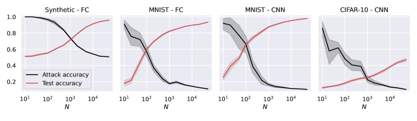
Figure 1: Test and attack accuracies as a function of the number of training samples $N$, for fully connected (FC, first two plots) and small convolutional neural networks (CNN, last two plots). In the first plot, we use synthetic (Gaussian) data with $d=1000$, and the labeling function is $g(x)=\textup{sign}(u^{\top}x)$ for a given $u\in\mathbb{R}^{d_{x}}$. As we are considering binary classification, the accuracy of random guessing is $0.5$. The other plots use subsets of the MNIST and CIFAR-10 datasets, with an external layer of noise added to the images (see Figure 2). The reconstruction attack queries the model only with the noise background, replacing all the other pixels with $0$. As we are considering $10$ classes, the accuracy of random guessing is $0.1$. We plot the average over 10 independent trials and the confidence band at 1 standard deviation.

2 Related Work

Private machine learning.

The phenomenon of information retrieval through partial knowledge of the data has been observed in question answering tasks in [10], where the approach is information theoretic. This setting is very natural in language models, as they are prone to memorize training set content [16, 15], and to hallucinate it at test time [52, 42]. Differential privacy [19] is a well established protocol that enables training deep learning models while maintaining privacy guarantees. This is achieved through the DPSGD [1] algorithm, which, despite continuous improvements [51, 5], still comes at a steep performance cost [1, 47]. Replacing sensitive data with suitably designed synthetic datasets can be a way to circumvent this problem. A recent line of work [8, 29, 9, 25] discusses efficient algorithms to succeed in this task, exploiting tools from high dimensional probability.

Stability.

The concept of algorithmic stability can be summarized as the influence of a single sample on the final trained model. The leave-one-out (error) stability has been formally linked to the generalization error in [28, 20, 33]. A wide range of variations on this object is discussed in the classical work [13], where the implications to generalization are demonstrated. A probabilistic point of view on this quantity has been named memorization in the related literature [22, 23], which emphasizes the non-privatized state of samples for which the algorithm is not stable. Specifically, [22] theoretically proposes that stability might be detrimental for learning, in settings where the data distribution is heavy-tailed. This hypothesis is then supported empirically in [23]. In contrast, [33] proves that, if the generalization gap vanishes with the number of samples, the learning algorithm has to be leave-one-out stable.

Random Features and Neural Tangent Kernel.

The RF model introduced by [41] can be regarded as a two-layer neural network with random first layer weights. This model is theoretically appealing, as it is analytically tractable and offers deep-learning-like behaviours, such as double descent [30]. Our analysis relies on the spectral properties of the kernel induced by random features, in particular on its smallest eigenvalue, which was studied for deep networks with a single wide layer [38] and in the context of robustness [12]. The NTK can be regarded as the kernel obtained by linearizing a neural network around the initialization [26]. A popular line of work has analyzed its spectrum [21, 3, 50] and bounded its smallest eigenvalue [46, 38, 32, 11]. The behavior of the NTK is closely related to memorization [32], optimization [4, 18], generalization [6] and robustness [12] properties of deep neural networks.

3 Preliminaries

Notation.

Given a vector $v$, we denote by $\left\|v\right\|_{2}$ its Euclidean norm. Given $v\in\mathbb{R}^{d_{v}}$ and $u\in\mathbb{R}^{d_{u}}$, we denote by $v\otimes u\in\mathbb{R}^{d_{v}d_{u}}$ their Kronecker product. Given a matrix $A\in\mathbb{R}^{m\times n}$, we denote by $P_{A}\in\mathbb{R}^{n\times n}$ the projector over $\textrm{Span}\{\operatorname{rows}(A)\}$. All the complexity notations $\Omega(\cdot)$, $\mathcal{O}(\cdot)$, $o(\cdot)$ and $\Theta(\cdot)$ are understood for sufficiently large data size $N$, input dimension $d$, number of neurons $k$, and number of parameters $p$. We indicate with $C,c>0$ numerical constants, independent of $N,d,k,p$.

Setting.

Let $(Z,G)$ be a labelled training dataset, where $Z=[z_{1},\ldots,z_{N}]^{\top}\in\mathbb{R}^{N\times d}$ contains the training data (sampled i.i.d. from a distribution $P_{Z}$) on its rows and $G=(g_{1},\ldots,g_{N})\in\mathbb{R}^{N}$ contains the corresponding labels. We assume the label $g_{i}$ to be a deterministic function of the sample $z_{i}$. Let $\varphi:\mathbb{R}^{d}\to\mathbb{R}^{p}$ be a generic feature map, from the input space to a feature space of dimension $p$. We consider the following generalized linear model

$$f(z,\theta)=\varphi(z)^{\top}\theta,$$ (3.1)

where $\varphi(z)\in\mathbb{R}^{p}$ is the feature vector associated with the input sample $z$, and $\theta\in\mathbb{R}^{p}$ is the set of the trainable parameters of the model. Our supervised learning setting involves minimizing the empirical risk, which, for a quadratic loss, can be formulated as

$$\mathop{\rm min}\nolimits_{\theta}\left\|\varphi(Z)^{\top}\theta-G\right\|_{2}^{2}.$$ (3.2)

Here, $\varphi(Z)\in\mathbb{R}^{N\times p}$ is the feature matrix, containing $\varphi(z_{i})$ in its $i$-th row. From now on, we use the shorthands $\Phi:=\varphi(Z)$ and $K:=\Phi\Phi^{\top}\in\mathbb{R}^{N\times N}$, where $K$ denotes the kernel associated with the feature map. If we assume $K$ to be invertible (i.e., the model is able to fit any set of labels $G$), it is well known that gradient descent converges to the interpolator which is the closest in $\ell_{2}$ norm to the initialization, see e.g. [24]. In formulas,

$$\theta^{*}=\theta_{0}+\Phi^{+}(G-f(Z,\theta_{0})),$$ (3.3)

where $\theta^{*}$ is the gradient descent solution, $\theta_{0}$ is the initialization, $f(Z,\theta_{0})=\Phi^{\top}\theta_{0}$ the output of the model (3.1) at initialization, and $\Phi^{+}:=\Phi^{\top}K^{-1}$ the Moore-Penrose inverse. Let $z\sim P_{Z}$ be an independent test sample. Then, we define the generalization error of the trained model as

$$\mathcal{R}=\mathbb{E}_{z\sim P_{Z}}\left[\left(f(z,\theta^{*})-g_{z}\right)^{2}\right],$$ (3.4)

where $g_{z}$ denotes the ground-truth label of the test sample $z$.

Stability.

For our discussion, it will be convenient to introduce quantities related to “incomplete” datasets. In particular, we indicate with $\Phi_{-1}\in\mathbb{R}^{(N-1)\times p}$ the feature matrix of the training set without the first sample $z_{1}$. In other words, $\Phi_{-1}$ is equivalent to $\Phi$, without the first row. Similarly, using (3.3), we indicate with $\theta_{-1}^{*}:=\theta_{0}+\Phi_{-1}^{+}\left(G_{-1}-f(Z_{-1},\theta_{0})\right)$ the set of parameters the algorithm would have converged to if trained over $(Z_{-1},G_{-1})$, the original dataset without the first pair sample-label $(z_{1},g_{1})$. We can now proceed with the definition of our notion of “stability”.

Definition 3.1.

Let $\theta^{*}$ ($\theta^{*}_{-1}$) be the parameters of the model $f$ given by (3.1) trained on the dataset $Z$ ($Z_{-1}$), as in (3.3). We define the stability $\mathcal{S}_{z_{1}}:\mathbb{R}^{d}\to\mathbb{R}$ with respect to the training sample $z_{1}$ as

$$\mathcal{S}_{z_{1}}:=f(\cdot,\theta^{*})-f(\cdot,\theta_{-1}^{*}).$$ (3.5)

This quantity indicates how the trained model changes if we add $z_{1}$ to the dataset $Z_{-1}$. Notice that, if the training algorithm completely fits the data (as in (3.3)), we have $\mathcal{S}_{z_{1}}(z_{1})=g_{1}-f(z_{1},\theta_{-1}^{*})$. This, readily implies that

$$\mathbb{E}_{z_{1}\sim P_{Z}}\left[\mathcal{S}^{2}_{z_{1}}(z_{1})\right]=\mathbb{E}_{z_{1}\sim P_{Z}}\left[\left(f(z_{1},\theta_{-1}^{*})-g_{1}\right)^{2}\right]=\mathbb{E}_{z\sim P_{Z}}\left[\left(f(z,\theta_{-1}^{*})-g_{z}\right)^{2}\right]=:\mathcal{R}_{Z_{-1}},$$ (3.6)

where the purpose of the second step is just to match the notation used in (3.4) and $\mathcal{R}_{Z_{-1}}$ denotes the generalization error of the algorithm that uses $Z_{-1}$ as training set.

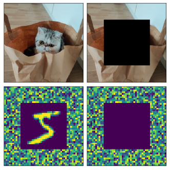
Figure 2: Example of a training sample $z$ (top-left) and its masked counterpart $z^{m}$ (top-right). In the experimental setting, we add a surrounding noise background ($y$) around the original images ($x$) before training (bottom-left). The attack consists in querying the trained model only with the noise component (bottom-right).

The connection between stability and generalization was thoroughly analyzed in the classical work [13], where different notions of stability are shown to imply upper bounds on the generalization gap of learning algorithms. In particular, if the cost function is limited from above, Theorem 11 of [13] proves that the condition $\mathbb{E}_{Z}\left[\mathcal{S}^{2}_{z_{1}}(z_{1})\right]\leq\beta$ (referred to as $\beta$-pointwise hypothesis stability in Definition 4) implies an upper bound on the generalization error. Our perspective is different, as we consider the trade-off between privacy and generalization. For this purpose, Definition 3.1 is convenient, as it makes stability the perfect bridge to draw the aforementioned trade-off.

Structure of the data and reconstruction attack.

Assume that the input samples can be decomposed in two independent components, i.e., $z\equiv[x,y]$. With this notation, we mean that the vector $z\in\mathbb{R}^{d}$ is the concatenation of $x\in\mathbb{R}^{d_{x}}$ and $y\in\mathbb{R}^{d_{y}}$, with $d_{x}+d_{y}=d$. Here, $x$ represents the part of the input that is useful to accomplish the task (e.g., the cat in top-left image of Figure 2), while $y$ can be regarded as noise (e.g., the background in the same image). Formally, we assume that, for $i\in\{1,\ldots,N\}$, $g_{i}=g(x_{i})$, where $g$ is a deterministic labelling function, which means that the label depends only on $x$ (and it is independent of $y$).

In practice, the noise component $y$ cannot be easily removed from the training dataset. Hence, the algorithm may overfit to it, thus learning the spurious correlations between the noise $y_{i}$ contained in the $i$-th sample and the corresponding label $g_{i}$. At this point, an attacker might exploit this phenomenon to reconstruct the label $g_{i}$, by simply querying the model with the noise component $y_{i}$. In our theoretical analysis, we assume the attacker to have access to a masked sample $z^{m}_{i}(x)=[x,y_{i}]$, i.e., a version of $z_{i}$ in which the component $x_{i}$ is replaced with an independent sample $x$ taken from the same distribution. We do the same in the synthetic setting of the numerical experiments, while for MNIST and CIFAR-10 we just set $x$ to $0$ for simplicity, see Figure 2 for an illustration. Our goal is to understand whether the output of the model evaluated on such query, i.e., $f(z^{m}_{i},\theta^{*})$, provides information about the ground-truth label $g(x_{i})$ of the $i$-th sample. From now on, we assume that the attack is aimed towards the first sample $z_{1}$. This is without loss of generality, as our setting is symmetric with respect to the ordering of the training data.

4 Stability, Generalization and Privacy

Stability and feature alignment.

Our goal is to quantify how much information about $g(x_{1})$ the attacker can recover through a generic query $z$. To do so, we relate $f(z,\theta^{*})$ to the model evaluated on the original sample $z_{1}$. It turns out that, for generalized linear regression, under mild conditions on the feature map $\varphi$, this can be elegantly done via the notion of stability of Definition 3.1.

Lemma 4.1.

Let $\varphi:\mathbb{R}^{d}\to\mathbb{R}^{p}$ be a generic feature map, such that the induced kernel $K\in\mathbb{R}^{N\times N}$ on the training set is invertible. Let $z_{1}\in\mathbb{R}^{d}$ be an element of the training dataset $Z$, and $z\in\mathbb{R}^{d}$ a generic test sample. Let $P_{\Phi_{-1}}$ be the projector over $\textrm{Span}\{\operatorname{rows}(\Phi_{-1})\}$, and $\mathcal{S}_{z_{1}}$ be the stability with respect to $z_{1}$, as in Definition 3.1. Let us denote by

$$\mathcal{F}_{\varphi}(z,z_{1}):=\frac{\varphi(z)^{\top}P_{\Phi_{-1}}^{\perp}\varphi(z_{1})}{\left\|P_{\Phi_{-1}}^{\perp}\varphi(z_{1})\right\|_{2}^{2}}$$ (4.1)

the feature alignment between $z$ and $z_{1}$. Then, we have

$$\mathcal{S}_{z_{1}}(z)=\mathcal{F}_{\varphi}(z,z_{1})\,\mathcal{S}_{z_{1}}(z_{1}).$$ (4.2)

The idea of the argument is to express $P_{\Phi}$ as $P_{\Phi_{-1}}$ plus the projector over the span of $P_{\Phi_{-1}}^{\perp}\varphi(z_{1})$, by leveraging the Gram-Schmidt decomposition of $P_{\Phi}$. The proof is deferred to Appendix B.

In words, Lemma 4.1 relates the stability with respect to $z_{1}$ evaluated on the two samples $z$ and $z_{1}$ through the quantity $\mathcal{F}_{\varphi}(z,z_{1})$, which captures the similarity between $z$ and $z_{1}$ in the feature space induced by $\varphi$. As a sanity check, the feature alignment between any sample and itself is equal to one, which trivializes (4.2). Then, as $z$ and $z_{1}$ become less aligned, the stability $\mathcal{S}_{z_{1}}(z)=f(z,\theta^{*})-f(z,\theta^{*}_{-1})$ starts to differ from $\mathcal{S}_{z_{1}}(z_{1})=f(z_{1},\theta^{*})-f(z_{1},\theta^{*}_{-1})$, as described quantitatively by (4.2). We note that the feature alignment also depends on the rest of the training set $Z_{-1}$, as $Z_{-1}$ implicitly appears in the projector $P_{\Phi_{-1}}^{\perp}$. We also remark that the invertibility of $K$ directly implies that the denominator in (4.1) is different from zero, see Lemma B.1.

Generalization and privacy.

Armed with Lemma 4.1, we now aim to characterize how powerful the attack query $f(z^{m}_{1},\theta^{*})$ can be. Let us replace $\mathcal{F}_{\varphi}(z^{m}_{1},z_{1})$ with a constant $\gamma_{\varphi}>0$, independent from $z_{1}$.This passage will be rigorously justified in the following Sections 5 and 6, where we prove the concentration of $\mathcal{F}_{\varphi}(z^{m}_{1},z_{1})$ for the RF and NTK model, respectively. By replacing $F_{\varphi}(z^{m}_{1},z_{1})$ with $\gamma_{\varphi}$ in (4.2) and using the definition of stability in (3.5), we get

$$f(z_{1}^{m},\theta^{*})=f(z_{1}^{m},\theta^{*}_{-1})+\gamma_{\varphi}\,\mathcal{S}_{z_{1}}(z_{1})=f(z_{1}^{m},\theta^{*}_{-1})+\gamma_{\varphi}\left(g_{1}-f(z_{1},\theta^{*}_{-1})\right).$$ (4.3)

Note that $f(z_{1}^{m},\theta^{*}_{-1})$ is independent from $g_{1}$, as it doesn’t depend on $x_{1}$. Therefore, if the algorithm is stable, in the sense that $\mathcal{S}_{z_{1}}(z_{1})$ is small, then it will also be private, as $f(z_{1}^{m},\theta^{*})$ has little dependence on $g_{1}$. Conversely, if $\mathcal{S}_{z_{1}}(z_{1})$ grows, then $f(z_{1}^{m},\theta^{*})$ will start picking up the correlation with $g_{1}$. More concretely, we can look at the covariance between $f(z_{1}^{m},\theta^{*})$ and $g_{1}$, in the probability space of $z_{1}$:

$$\textup{Cov}\left(f(z^{m}_{1},\theta^{*}),g_{1}\right)=\gamma_{\varphi}\,\textup{Cov}\left(S_{z_{1}}(z_{1}),g_{1}\right)\leq\gamma_{\varphi}\,\sqrt{\textup{Var}\left(S_{z_{1}}(z_{1})\right)\textup{Var}\left(g_{1}\right)}\leq\gamma_{\varphi}\,\sqrt{\mathcal{R}_{Z_{-1}}}\sqrt{\textup{Var}\left(g_{1}\right)}.$$ (4.4)

Here, the first step uses (4.3), and the independence between $f(z_{1}^{m},\theta^{*}_{-1})$ and $g_{1}$, the second step is an application of Cauchy-Schwarz inequality, and the last step follows from (3.6). Let us now focus on the RHS of (4.4). While $\sqrt{\textup{Var}\left(g_{1}\right)}$ is a simple scaling factor, $\gamma_{\varphi}$ and $\sqrt{\mathcal{R}_{Z_{-1}}}$ lead to an interesting interpretation: we expect the attack to become more powerful as the similarity between $z^{m}_{1}$ and $z_{1}$ – formalized by $\mathcal{F}_{\varphi}(z^{m}_{1},z_{1})$ – increases, and less effective as the generalization error of the model decreases. In fact, the potential threat hinges on the model overfitting the $y$-component at training time. This overfitting would both cause higher generalization error, and higher chances of recovering $g_{1}$ given only $y_{1}$.

5 Main Result for Random Features

The random features (RF) model takes the form

$$f_{\textup{RF}}(z,\theta)=\varphi_{\textup{RF}}(z)^{\top}\theta,\qquad\varphi_{\textup{RF}}(z)=\phi(Vz),$$ (5.1)

where $V$ is a $k\times d$ matrix, such that $V_{i,j}\mathbin{\overset{}{\sim}}_{\rm i.i.d.}\mathcal{N}(0,1/d)$, and $\phi$ is an activation function applied component-wise. The number of parameters of this model is $k$, as $V$ is fixed and $\theta\in\mathbb{R}^{k}$ contains the trainable parameters. We will make the following assumptions on the data and on the model.

Assumption 1 (Data distribution).

The input data $(z_{1},\ldots,z_{N})$ are $N$ i.i.d. samples from the distribution $P_{Z}=P_{X}\times P_{Y}$, such that every sample $z_{i}\in\mathbb{R}^{d}$ can be written as $z_{i}=[x_{i},y_{i}]$, with $x_{i}\in\mathbb{R}^{d_{x}}$, $y_{i}\in\mathbb{R}^{d_{y}}$ and $d=d_{x}+d_{y}$. We assume that $x_{i}\sim P_{X}$ is independent of $y_{i}\sim P_{Y}$, and the following properties hold:

1. $\left\|x\right\|_{2}=\sqrt{d_{x}}$, and $\left\|y\right\|_{2}=\sqrt{d_{y}}$, i.e., the data have normalized norm.

2. $\mathbb{E}[x]=0$, and $\mathbb{E}[y]=0$, i.e., the data are centered.

3. Both $P_{X}$ and $P_{Y}$ satisfy the Lipschitz concentration property.

The first two assumptions can be achieved by simply pre-processing the raw data, and they could potentially be relaxed as in Assumption 1 of [11] at the cost of a more involved argument. For the third assumption (formally defined and discussed in Appendix A), we remark that the family of Lipschitz concentrated distributions covers a number of important cases, e.g., standard Gaussian [49], uniform on the sphere/hypercube [49], or data obtained via a Generative Adversarial Network (GAN) [44]. This requirement is common in the related literature [11, 12, 14, 38] and, in fact, it is often replaced by a stronger requirement (e.g., data uniform on the sphere), see [32].

Assumption 2 (Over-parameterization and high-dimensional data).

$$N\log^{3}N=o(k),\qquad\sqrt{d}\log d=o(k),\qquad k\log^{4}k=o\left(d^{2}\right).$$ (5.2)

In words, the first condition in (5.2) requires the number of neurons $k$ to scale faster than the number of data points $N$. This over-parameterization leads to a lower bound on the smallest eigenvalue of the kernel induced by the feature map, which in turn implies that the model perfectly interpolates the data, as required to write (3.3). We note that this over-parameterized regime has also been shown to achieve minimum test error [30]. Combining the second and third conditions in (5.2), we have that $k$ can scale between $\sqrt{d}$ and $d^{2}$ (up to $\log$ factors). Finally, merging the first and third condition gives that $d^{2}$ scales faster than $N$. We notice that this holds for standard datasets, e.g., MNIST ($N=6\cdot 10^{4}$, $d=784$), CIFAR-10 ($N=5\cdot 10^{4}$, $d=3\cdot 32^{2}$), and ImageNet ($N=1.4\cdot 10^{7}$, $d=2\cdot 10^{5}$).

Assumption 3 (Activation function).

The activation function $\phi$ is a non-linear $L$-Lipschitz function.

This requirement is satisfied by common activations, e.g., ReLU, sigmoid, or $\tanh$.

We denote by $\mu_{l}$ the $l$-th Hermite coefficient of $\phi$ (see Appendix A.1 for details on Hermite expansions). We remark that the invertibility of the kernel $K_{\textup{RF}}$ induced by the feature map in (5.1), which is necessary to apply Lemma 4.1 and use (4.1), follows from Lemma D.2. At this point, we are ready to state our main result for the random features model, whose full proof is contained in Appendix D.

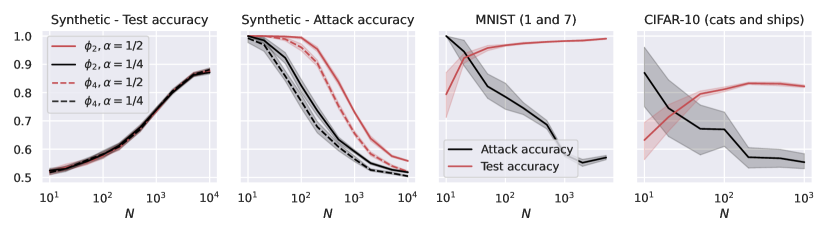
Figure 3: Test and attack accuracies as a function of the number of training samples $N$, for various binary classification tasks. In the first two plots, we consider the RF model in (5.1) with $k=10^{5}$ trained over Gaussian data with $d=1000$. The labeling function is $g(x)=\textup{sign}(u^{\top}x)$ for a given $u\in\mathbb{R}^{d_{x}}$. We repeat the experiments for $\alpha=\{0.25,0.5\}$, and for the two activations $\phi_{2}=h_{1}+h_{2}$ and $\phi_{4}=h_{1}+h_{4}$, where $h_{i}$ denotes the $i$-th Hermite polynomial (see Appendix A.1). In the last two plots, we consider the same model with ReLU activation, trained over two MNIST and CIFAR-10 classes. We add a noise background whose width is $10$ pixels for MNIST and $8$ pixels for CIFAR-10 (see Figure 2). The reconstruction attack queries the model only with the noise background, replacing all the other pixels with $0$, and takes the sign of the output. Note that, as we are considering binary classification, an accuracy of 0.5 is achieved by random guessing. We plot the average over 10 independent trials and the confidence band at 1 standard deviation.

Theorem 1.

Let Assumptions 1, 2, and 3 hold, and let $x\sim P_{X}$ be sampled independently from everything. Consider querying the trained RF model (5.1) with $z_{1}^{m}=[x,y_{1}]$. Let $\alpha=d_{y}/d$ and $\mathcal{F}_{\textup{RF}}(z_{1}^{m},z_{1})$ be the feature alignment between $z_{1}^{m}$ and $z_{1}$, as defined in (4.1). Then,

$$\left|\mathcal{F}_{\textup{RF}}(z_{1}^{m},z_{1})-\gamma_{\textup{RF}}\right|=o(1),$$ (5.3)

with probability at least $1-\exp(-c\log^{2}N)$ over $V$, $Z$ and $x$, where $c$ is an absolute constant, and $\gamma_{\textup{RF}}\leq 1$ does not depend on $z_{1}$ and $x$. Furthermore, we have

$$\gamma_{\textup{RF}}>\frac{\sum_{l=2}^{+\infty}\mu_{l}^{2}\alpha^{l}}{\sum_{l=1}^{+\infty}\mu_{l}^{2}}-o(1),$$ (5.4)

with probability at least $1-\exp(-c\log^{2}N)$ over $V$, and $Z_{-1}$, where $c$ is an absolute constant, i.e., $\gamma_{\textup{RF}}$ is bounded away from $0$ with high probability.

The combination of Theorem 1 and Lemma 4.1 unveils a remarkable proportionality relation between stability and privacy: the more the algorithm is stable (and, therefore, capable of generalizing), the smaller the effect of the reconstruction attack. The proportionality constant $\gamma_{\textup{RF}}$ is between $\frac{\sum_{l=2}^{+\infty}\mu_{l}^{2}\alpha^{l}}{\sum_{l=1}^{+\infty}\mu_{l}^{2}}>0$ and $1$. In particular, the lower bound increases with $\alpha$ – which is expected, since $\alpha$ represents the fraction of the input to which the attacker has access – and it depends in a non-trivial way on the activation function via its Hermite coefficients.

All these effects are clearly displayed in Figure 3 for binary classification tasks involving synthetic (first two plots) and standard (last two plots) datasets. Specifically, as the number of samples $N$ increases, the test accuracy increases and, correspondingly, the effect of the reconstruction attack decreases. Furthermore, for the synthetic dataset, while the test accuracy does not appear to depend on $\alpha$ and on the activation function, the success of the attack increases with $\alpha$ and by taking an activation function with dominant low-order Hermite coefficients, as predicted by (5.4).

Proof sketch.

We set $\gamma_{\textup{RF}}:=\mathbb{E}_{z_{1},z_{1}^{m}}[\varphi_{\textup{RF}}(z_{1}^{m})^{\top}P_{\Phi_{-1}}^{\perp}\varphi_{\textup{RF}}(z_{1})]/\mathbb{E}_{z_{1}}[\|P_{\Phi_{-1}}^{\perp}\varphi_{\textup{RF}}(z_{1})\|_{2}^{2}]$. Here, $P_{\Phi_{-1}}$ denotes the projector over $\textrm{Span}\{\operatorname{rows}(\Phi_{\textup{RF},-1})\}$ and $\Phi_{\textup{RF},-1}$ is the RF feature matrix after removing the first row. With this choice, the numerator and denominator of $\gamma_{\textup{RF}}$ equal the expectations of the corresponding quantities appearing in $\mathcal{F}_{\textup{RF}}(z_{1}^{m},z_{1})$. Thus, the concentration result in (5.3) can be obtained by applying the general form of the Hanson-Wright inequality in [2], see Lemma D.7.

The upper bound $\gamma_{\textup{RF}}\leq 1$ follows from an application of Cauchy-Schwarz inequality. In contrast, the lower bound is more involved and it is obtained via the following three steps:

Step 1: Centering the feature map $\varphi_{\textup{RF}}$. We extract the term $\mathbb{E}_{V}\left[\phi(Vz)\right]$ from the expression of $\mathcal{F}_{\textup{RF}}$ and we show that it can be neglected, due to the specific structure of $P_{\Phi_{-1}}^{\perp}$. Specifically, letting $\tilde{\varphi}_{\textup{RF}}(z):=\varphi_{\textup{RF}}(z)-\mathbb{E}_{V}\left[\varphi_{\textup{RF}}(z)\right]$, we have

$$\mathcal{F}_{\textup{RF}}(z_{1}^{m},z_{1})\simeq\frac{\tilde{\varphi}_{\textup{RF}}(z_{1}^{m})^{\top}P_{\Phi_{-1}}^{\perp}\tilde{\varphi}_{\textup{RF}}(z_{1})}{\left\|P_{\Phi_{-1}}^{\perp}\tilde{\varphi}_{\textup{RF}}(z_{1})\right\|_{2}^{2}}=\frac{\tilde{\varphi}_{\textup{RF}}(z_{1}^{m})^{\top}\tilde{\varphi}_{\textup{RF}}(z_{1})-\tilde{\varphi}_{\textup{RF}}(z_{1}^{m})^{\top}P_{\Phi_{-1}}\tilde{\varphi}_{\textup{RF}}(z_{1})}{\left\|P_{\Phi_{-1}}^{\perp}\tilde{\varphi}_{\textup{RF}}(z_{1})\right\|_{2}^{2}},$$ (5.5)

where $\simeq$ denotes an equality up to a $o(1)$ term. This is formalized in Lemma D.3.

Step 2: Linearization of the centered feature map $\tilde{\varphi}_{\textup{RF}}$. We consider the terms $\tilde{\varphi}_{\textup{RF}}(z_{1}^{m}),\tilde{\varphi}_{\textup{RF}}(z_{1})$ that multiply $P_{\Phi_{-1}}$ in the RHS of (5.5), and we show that they are well approximated by their first-order Hermite expansions ($\mu_{1}Vz_{1}^{m}$ and $\mu_{1}Vz_{1}$, respectively). In fact, the rest of the Hermite series scales at most as $N/d^{2}$, which is negligible due to Assumption 2. Specifically, Lemma D.4 implies

$$\frac{\tilde{\varphi}_{\textup{RF}}(z_{1}^{m})^{\top}\tilde{\varphi}_{\textup{RF}}(z_{1})-\tilde{\varphi}_{\textup{RF}}(z_{1}^{m})^{\top}P_{\Phi_{-1}}\tilde{\varphi}_{\textup{RF}}(z_{1})}{\left\|P_{\Phi_{-1}}^{\perp}\tilde{\varphi}_{\textup{RF}}(z_{1})\right\|_{2}^{2}}\simeq\frac{\tilde{\varphi}_{\textup{RF}}(z_{1}^{m})^{\top}\tilde{\varphi}_{\textup{RF}}(z_{1})-\mu_{1}^{2}(Vz_{1}^{m})^{\top}P_{\Phi_{-1}}(Vz_{1})}{\left\|P_{\Phi_{-1}}^{\perp}\tilde{\varphi}_{\textup{RF}}(z_{1})\right\|_{2}^{2}}.$$ (5.6)

Step 3: Lower bound in terms of $\alpha$ and $\{\mu_{l}\}_{l\geq 2}$. To conclude, we express the RHS of (5.6) as follows:

$$\frac{\tilde{\varphi}_{\textup{RF}}(z_{1}^{m})^{\top}\tilde{\varphi}_{\textup{RF}}(z_{1})-\mu_{1}^{2}(Vz_{1}^{m})^{\top}(Vz_{1})+\mu_{1}^{2}(Vz_{1}^{m})^{\top}P_{\Phi_{-1}}^{\perp}(Vz_{1})}{\left\|\tilde{\varphi}_{\textup{RF}}(z_{1})\right\|_{2}^{2}-\left\|P_{\Phi_{-1}}\tilde{\varphi}_{\textup{RF}}(z_{1})\right\|_{2}^{2}}$$ (5.7)

$$\hskip 80.00012pt\gtrsim\frac{\tilde{\varphi}_{\textup{RF}}(z_{1}^{m})^{\top}\tilde{\varphi}_{\textup{RF}}(z_{1})-\mu_{1}^{2}(Vz_{1}^{m})^{\top}(Vz_{1})}{\left\|\tilde{\varphi}_{\textup{RF}}(z_{1})\right\|_{2}^{2}}\simeq\frac{\sum_{l=2}^{+\infty}\mu_{l}^{2}\alpha^{l}}{\sum_{l=1}^{+\infty}\mu_{l}^{2}}>0,$$

where $\gtrsim$ denotes an inequality up to a $o(1)$ term. The expression in the first line equals the RHS of (5.6) as $P_{\Phi_{-1}}=I-P_{\Phi_{-1}}^{\perp}$. Next, we show that $\mu_{1}^{2}(Vz_{1}^{m})^{\top}P_{\Phi_{-1}}^{\perp}(Vz_{1})$ is equal to $\mu_{1}^{2}(V[y_{1},0])^{\top}P_{\Phi_{-1}}^{\perp}(V[y_{1},0])$ (which corresponds to the common noise part in the samples $z_{1},z_{1}^{m}$) plus a vanishing term, see Lemma D.5. As $\mu_{1}^{2}(V[y_{1},0])^{\top}P_{\Phi_{-1}}^{\perp}(V[y_{1},0])\geq 0$, the inequality in the second line follows. Finally, the last step is obtained by showing concentration over $V$ of the numerator and denominator. The expression on the RHS of (5.7) is strictly positive as $\alpha>0$ and $\phi$ is non-linear by Assumption 3.

6 Main Result for NTK Regression

We consider the following two-layer neural network

$$f_{\textup{NN}}(z,w)=\sum_{i=1}^{k}\phi\left(W_{i:}z\right).$$ (6.1)

Here, the hidden layer contains $k$ neurons; $\phi$ is an activation function applied component-wise; $W\in\mathbb{R}^{k\times d}$ denotes the weights of the hidden layer; $W_{i:}$ denotes the $i$-th row of $W$; and we set the $k$ weights of the second layer to $1$. We indicate with $w$ the vector containing the parameters of this model, i.e., $w=[\text{vec}(W)]\in\mathbb{R}^{p}$, with $p=kd$. We initialize the network with standard (e.g., He’s or LeCun’s) initialization, i.e., $[W_{0}]_{i,j}\mathbin{\overset{}{\sim}}_{\rm i.i.d.}\mathcal{N}(0,1/d)$. Now, the NTK regression model takes the form

$$f_{\textup{NTK}}(z,\theta)=\varphi_{\textup{NTK}}(z)^{\top}\theta,\qquad\varphi_{\textup{NTK}}(z)=\nabla_{w}f_{\textup{NN}}(z,w)|_{w=w_{0}}.$$ (6.2)

Here, the vector of trainable parameters is $\theta\in\mathbb{R}^{p}$, with $p=kd$, which is initialized with $\theta_{0}=w_{0}=[\text{vec}(W_{0})]$. We remark that this is the same model considered in [12, 17, 32], and $f_{\textup{NTK}}(z,\theta)$ corresponds to the linearization of $f_{\textup{NN}}(z,w)$ around the initial point $w_{0}$ [7, 26]. An application of the chain rule gives

$$\varphi_{\textup{NTK}}(z)=z\otimes\phi^{\prime}(W_{0}z).$$ (6.3)

Throughout this section, we make the following assumptions.

Assumption 4 (Over-parameterization and topology).

$$N\log^{8}N=o(kd),\qquad N>d,\qquad k=\mathcal{O}\left(d\right).$$ (6.4)

The first condition provides the weakest (up to $\log$ factors) possible requirement on the number of parameters of a model that guarantees interpolation for generic data points [11]. The second condition is rather mild (it is easily satisfied by standard datasets) and purely technical. The third condition is required to lower bound the smallest eigenvalue of the kernel induced by the feature map, and a stronger requirement, i.e., the strict inequality $k<d$, has appeared in prior work [35, 36, 37].

Assumption 5 (Activation function).

The activation function $\phi$ is a non-linear function with $L$-Lipschitz first order derivative $\phi^{\prime}$.

This requirements is satisfied by common activations, e.g. smoothed ReLU, sigmoid, or $\tanh$.

We denote by $\mu^{\prime}_{l}$ the $l$-th Hermite coefficient of $\phi^{\prime}$. We remark that the invertibility of the kernel $K_{\textup{NTK}}$ induced by the feature map (6.2) follows from Lemma E.1. At this point, we are ready to state our main result for the NTK model, whose full proof is contained in Appendix E.

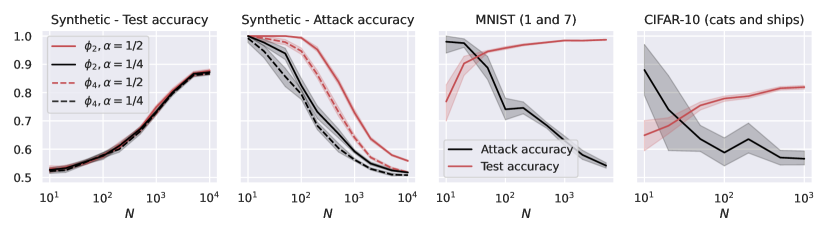
Figure 4: We consider the NTK model in (5.1) with $k=100$ and, in the first two plots, we repeat the experiments for activations whose derivatives are $\phi^{\prime}_{2}=h_{0}+h_{1}$ and $\phi^{\prime}_{4}=h_{0}+h_{3}$, where $h_{i}$ denotes the $i$-th Hermite polynomial (see Appendix A.1). The rest of the setup is similar to that of Figure 3.

Theorem 2.

Let Assumptions 1, 4, and 5 hold, and let $x\sim P_{X}$ be sampled independently from everything. Consider querying the trained NTK model (6.2) with $z_{1}^{m}=[x,y_{1}]$. Let $\alpha=d_{y}/d\in(0,1)$ and $\mathcal{F}_{\textup{NTK}}(z_{1}^{m},z_{1})$ be the feature alignment between $z_{1}^{m}$ and $z_{1}$, as defined in (4.1). Then,

$$\left|\mathcal{F}_{\textup{NTK}}(z_{1}^{m},z_{1})-\gamma_{\textup{NTK}}\right|=o(1),\qquad\mbox{where }\,\,\,0<\gamma_{\textup{NTK}}:=\alpha\,\frac{\sum_{l=1}^{+\infty}{\mu^{\prime}_{l}}^{2}\alpha^{l}}{\sum_{l=1}^{+\infty}{\mu^{\prime}_{l}}^{2}}<1,$$ (6.5)

with probability at least $1-N\exp(-c\log^{2}k)-\exp(-c\log^{2}N)$ over $Z$, $x$, and $W$, where $c$ is an absolute constant.

The combination of Theorem 2 and Lemma 4.1 describes a connection between stability and privacy, similar to that discussed for the RF model. In addition, for the NTK model, we are able to express the limit $\gamma_{\textup{NTK}}$ of the feature alignment in a closed form involving $\alpha$ and the Hermite coefficients of the derivative of the activation. The findings of Theorem 2 are clearly displayed in Figure 4: as $N$ increases, the test accuracy improves and the reconstruction attack becomes less effective; decreasing $\alpha$ or considering activations with dominant high-order Hermite coefficients also reduces the accuracy of the attack.

Proof sketch.

The argument is more direct than for the RF model since, in this case, we are able to express $\gamma_{\textup{NTK}}$ in closed form. We denote by $P_{\Phi_{-1}}$ the projector over the span of the rows of the NTK feature matrix $\Phi_{\textup{NTK},-1}$ without the first row. Then, the first step is to center the feature map $\varphi_{\textup{NTK}}$, which gives

$$\frac{\varphi_{\textup{NTK}}(z_{1}^{m})^{\top}P_{\Phi_{-1}}^{\perp}\varphi_{\textup{NTK}}(z_{1})}{\left\|P_{\Phi_{-1}}^{\perp}\varphi_{\textup{NTK}}(z_{1})\right\|_{2}^{2}}\simeq\frac{\tilde{\varphi}_{\textup{NTK}}(z_{1}^{m})^{\top}P_{\Phi_{-1}}^{\perp}\tilde{\varphi}_{\textup{NTK}}(z_{1})}{\left\|P_{\Phi_{-1}}^{\perp}\tilde{\varphi}_{\textup{NTK}}(z_{1})\right\|_{2}^{2}},$$ (6.6)

where $\tilde{\varphi}_{\textup{NTK}}(z):=z\otimes\left(\phi^{\prime}(W_{0}z)-\mathbb{E}_{W_{0}}\left[\phi^{\prime}(W_{0}z)\right]\right)$. While a similar step appeared in the analysis of the RF model, its implementation for NTK requires a different strategy. In particular, we exploit that the samples $z_{1}$ and $z_{1}^{m}$ are approximately contained in the span of the rows of $Z_{-1}$ (see Lemma E.4). As the rows of $Z_{-1}$ may not exactly span all $\mathbb{R}^{d}$, we resort to an approximation by adding a small amount of independent noise to every entry of $Z_{-1}$. The resulting perturbed dataset $\bar{Z}_{-1}$ satisfies $\textrm{Span}\{\operatorname{rows}(\bar{Z}_{-1})\}=\mathbb{R}^{d}$ (see Lemma E.3), and we conclude via a continuity argument with respect to the magnitude of the perturbation (see Lemmas E.2 and E.5).

The second step is to upper bound the terms $\left|\tilde{\varphi}_{\textup{NTK}}(z_{1}^{m})^{\top}P_{\Phi_{-1}}\tilde{\varphi}_{\textup{NTK}}(z_{1})\right|$ and $\left\|P_{\Phi_{-1}}\tilde{\varphi}_{\textup{NTK}}(z_{1})\right\|_{2}^{2}$, showing they have negligible magnitude, which gives

$$\frac{\tilde{\varphi}_{\textup{NTK}}(z_{1}^{m})^{\top}P_{\Phi_{-1}}^{\perp}\tilde{\varphi}_{\textup{NTK}}(z_{1})}{\left\|P_{\Phi_{-1}}^{\perp}\tilde{\varphi}_{\textup{NTK}}(z_{1})\right\|_{2}^{2}}\simeq\frac{\tilde{\varphi}_{\textup{NTK}}(z_{1}^{m})^{\top}\tilde{\varphi}_{\textup{NTK}}(z_{1})}{\left\|\tilde{\varphi}_{\textup{NTK}}(z_{1})\right\|_{2}^{2}}.$$ (6.7)

This is a consequence of the fact that, if $z\sim P_{Z}$ is independent from $Z_{-1}$, then $\tilde{\varphi}(z)$ is roughly orthogonal to $\textrm{Span}\{\operatorname{rows}(\Phi_{\textup{NTK},-1})\}$, see Lemma E.8.

Finally, the third step is to show the concentration over $W_{0}$ of the numerator and denominator of the RHS of (6.7), which allows us to conclude that

$$\frac{\tilde{\varphi}_{\textup{NTK}}(z_{1}^{m})^{\top}\tilde{\varphi}_{\textup{NTK}}(z_{1})}{\left\|\tilde{\varphi}_{\textup{NTK}}(z_{1})\right\|_{2}^{2}}\simeq\alpha\,\frac{\sum_{l=1}^{+\infty}{\mu^{\prime}_{l}}^{2}\alpha^{i}}{\sum_{l=1}^{+\infty}{\mu^{\prime}_{l}}^{2}}>0.$$ (6.8)

This is formalized in Lemma E.6, and the RHS of (6.8) is strictly positive as $\alpha>0$ and $\phi$ is non-linear by Assumption 5.

7 Conclusions

In this work, we provide a quantitative characterization of the accuracy of a family of powerful information recovery attacks. This characterization hinges on (i) the classical notion of stability of the model w.r.t. a training sample, and (ii) a novel notion of feature alignment $\mathcal{F}(z_{1},z_{1}^{m})$ between the target of the attack $z_{1}$ and the adversarial query $z_{1}^{m}$. By providing a precise analysis for this feature alignment, we unveil a rigorous connection between generalization and privacy (intended in terms of the protection against the aforementioned attacks). While the theoretical analysis focuses on generalized linear regression with random and NTK features, numerical results on different neural network architectures point to the generality of our findings, see Figure 1. Quantifying this generality – as well as going beyond the framework of empirical risk minimization (e.g., by considering differential privacy) – provides an exciting avenue for future work.

Appendix A Additional Notations and Remarks

Given a sub-exponential random variable $X$, let $\|X\|_{\psi_{1}}=\inf\{t>0\,\,:\,\,\mathbb{E}[\exp(|X|/t)]\leq 2\}$. Similarly, for a sub-Gaussian random variable, let $\|X\|_{\psi_{2}}=\inf\{t>0\,\,:\,\,\mathbb{E}[\exp(X^{2}/t^{2})]\leq 2\}$. We use the analogous definitions for vectors. In particular, let $X\in\mathbb{R}^{n}$ be a random vector, then $\left\|X\right\|_{\psi_{2}}:=\sup_{\left\|u\right\|_{2}=1}\left\|u^{\top}X\right\|_{\psi_{2}}$ and $\left\|X\right\|_{\psi_{1}}:=\sup_{\left\|u\right\|_{2}=1}\left\|u^{\top}X\right\|_{\psi_{1}}$. Notice that if a vector has independent, mean 0, sub-Gaussian (sub-exponential) entries, then it is sub-Gaussian (sub-exponential). This is a direct consequence of Hoeffding’s inequality and Bernstein’s inequality (see Theorems 2.6.3 and 2.8.2 in [49]).

We say that a random variable or vector respects the Lipschitz concentration property if there exists an absolute constant $c>0$ such that, for every Lipschitz continuous function $\tau:\mathbb{R}^{d}\to\mathbb{R}$, we have $\mathbb{E}|\tau(X)|<+\infty$, and for all $t>0$,

$$\mathbb{P}\left(\left|\tau(x)-\mathbb{E}_{X}[\tau(x)]\right|>t\right)\leq 2e^{-ct^{2}/\left\|\tau\right\|_{\mathrm{Lip}}^{2}}.$$ (A.1)

When we state that a random variable or vector $X$ is sub-Gaussian (or sub-exponential), we implicitly mean $\left\|X\right\|_{\psi_{2}}=\mathcal{O}\left(1\right)$, i.e. it doesn’t increase with the scalings of the problem. Notice that, if $X$ is Lipschitz concentrated, then $X-\mathbb{E}[X]$ is sub-Gaussian. If $X\in\mathbb{R}$ is sub-Gaussian and $\tau:\mathbb{R}\to\mathbb{R}$ is Lipschitz, we have that $\tau(X)$ is sub-Gaussian as well. Also, if a random variable is sub-Gaussian or sub-exponential, its $p$-th momentum is upper bounded by a constant (that might depend on $p$).

In general, we indicate with $C$ and $c$ absolute, strictly positive, numerical constants, that do not depend on the scalings of the problem, i.e. input dimension, number of neurons, or number of training samples. Their value may change from line to line.

Given a matrix $A$, we indicate with $A_{i:}$ its $i$-th row, and with $A_{:j}$ its $j$-th column. Given a square matrix $A$, we denote by $\lambda_{\rm min}\left(A\right)$ its smallest eigenvalue. Given a matrix $A$, we indicate with $\sigma_{\mathop{\rm min}\nolimits}(A)=\sqrt{\lambda_{\rm min}\left(A^{\top}A\right)}$ its smallest singular value, with $\left\lVert A\right\rVert_{\textup{op}}$ its operator norm (and largest singular value), and with $\left\|A\right\|_{F}$ its Frobenius norm ($\left\|A\right\|^{2}_{F}=\sum_{ij}A_{ij}^{2}$).

Given two matrices $A,B\in\mathbb{R}^{m\times n}$, we denote by $A\circ B$ their Hadamard product, and by $A\ast B=[(A_{1:}\otimes B_{1:}),\ldots,(A_{m:}\otimes B_{m:})]^{\top}\in\mathbb{R}^{m\times n^{2}}$ their row-wise Kronecker product (also known as Khatri-Rao product). We denote $A^{*2}=A\ast A$. We remark that $\left(A*B\right)\left(A*B\right)^{\top}=AA^{\top}\circ BB^{\top}$. We say that a matrix $A\in\mathbb{R}^{n\times n}$ is positive semi definite (p.s.d.) if it’s symmetric and for every vector $v\in\mathbb{R}^{n}$ we have $v^{\top}Av\geq 0$.

A.1 Hermite Polynomials

In this subsection, we refresh standard notions on the Hermite polynomials. For a more comprehensive discussion, we refer to [39]. The (probabilist’s) Hermite polynomials $\{h_{j}\}_{j\in\mathbb{N}}$ are an orthonormal basis for $L^{2}(\mathbb{R},\gamma)$, where $\gamma$ denotes the standard Gaussian measure. The following result holds.

Proposition A.1 (Proposition 11.31, [39]).

Let $\rho_{1},\rho_{2}$ be two standard Gaussian random variables, with correlation $\rho\in[-1,1]$. Then,

$$\mathbb{E}_{\rho_{1},\rho_{2}}\left[h_{i}(\rho_{1})h_{j}(\rho_{2})\right]=\delta_{ij}\rho^{i},$$ (A.2)

where $\delta_{ij}=1$ if $i=j$, and $0$ otherwise.

The first 5 Hermite polynomials are

$$h_{0}(\rho)=1,\quad h_{1}(\rho)=\rho,\quad h_{2}(\rho)=\frac{\rho^{2}-1}{\sqrt{2}},\quad h_{3}(\rho)=\frac{\rho^{3}-3\rho}{\sqrt{6}},\quad h_{4}(\rho)=\frac{\rho^{4}-6\rho^{2}+3}{\sqrt{24}}.$$ (A.3)

Proposition A.2 (Definition 11.34, [39]).

Every function $\phi\in L^{2}(\mathbb{R},\gamma)$ is uniquely expressible as

$$\phi(\rho)=\sum_{i\in\mathbb{N}}\mu^{\phi}_{i}h_{i}(\rho),$$ (A.4)

where the real numbers $\mu^{\phi}_{i}$’s are called the Hermite coefficients of $\phi$, and the convergence is in $L^{2}(\mathbb{R},\gamma)$. More specifically,

$$\lim_{n\to+\infty}\left\|\left(\sum_{i=0}^{n}\mu^{\phi}_{i}h_{i}(\rho)\right)-\phi(\rho)\right\|_{L^{2}(\mathbb{R},\gamma)}=0.$$ (A.5)

This readily implies the following result.

Proposition A.3.

Let $\rho_{1},\rho_{2}$ be two standard Gaussian random variables with correlation $\rho\in[-1,1]$, and let $\phi,\tau\in L^{2}(\mathbb{R},\gamma)$. Then,

$$\mathbb{E}_{\rho_{1},\rho_{2}}\left[\phi(\rho_{1})\tau(\rho_{2})\right]=\sum_{i\in\mathbb{N}}\mu^{\phi}_{i}\mu^{\tau}_{i}\rho^{i}.$$ (A.6)

Appendix B Proof of Lemma 4.1

We start by refreshing some useful notions of linear algebra. Let $A\in\mathbb{R}^{N\times p}$ be a matrix, with $p\geq N$, and $A_{-1}\in\mathbb{R}^{(N-1)\times p}$ be obtained from $A$ after removing the first row. We assume $AA^{\top}$ to be invertible, i.e., the rows of $A$ are linearly independent. Thus, also the rows of $A_{-1}$ are linearly independent, implying that $A_{-1}A_{-1}^{\top}$ is invertible as well. We indicate with $P_{A}\in\mathbb{R}^{p\times p}$ the projector over $\textrm{Span}\{\operatorname{rows}(A)\}$, and we correspondingly define $P_{A_{-1}}\in\mathbb{R}^{p\times p}$. As $AA^{\top}$ is invertible, we have that $\textrm{rank}(A)=N$.

By singular value decomposition, we have $A=UDO^{\top}$, where $U\in\mathbb{R}^{N\times N}$ and $O\in\mathbb{R}^{p\times p}$ are orthogonal matrices, and $D\in\mathbb{R}^{N\times p}$ contains the (all strictly positive) singular values of $A$ in its “left” diagonal, and is 0 in every other entry. Let us define $O_{1}\in\mathbb{R}^{N\times p}$ as the matrix containing the first $N$ rows of $O$. This notation implies that if $O_{1}u=0$ for $u\in\mathbb{R}^{p}$, then $Au=0$, i.e., $u\in\textrm{Span}\{\operatorname{rows}(A)\}^{\perp}$. The opposite implication is also true, which implies that $\textrm{Span}\{\operatorname{rows}(A)\}=\textrm{Span}\{\operatorname{rows}(O_{1})\}$. As the rows of $O_{1}$ are orthogonal, we can then write

$$P_{A}=O_{1}^{\top}O_{1}.$$ (B.1)

We define $D_{s}\in\mathbb{R}^{N\times N}$, as the square, diagonal, and invertible matrix corresponding to the first $N$ columns of $D$. Let’s also define $I_{N}\in\mathbb{R}^{p\times p}$ as the matrix containing 1 in the first $N$ entries of its diagonal, and 0 everywhere else. We have

$$P_{A}= O_{1}^{\top}O_{1}=OI_{N}O^{\top}$$ (B.2)

$$= OD^{\top}D_{s}^{-2}DO^{\top}=OD^{\top}U^{\top}UD_{s}^{-2}U^{\top}UDO^{\top}$$

$$= A^{\top}\left(UD_{s}^{2}U^{\top}\right)^{-1}A=A^{\top}\left(UDO^{\top}OD^{\top}U^{\top}\right)^{-1}A$$

$$= A^{\top}\left(AA^{\top}\right)^{-1}A\equiv A^{+}A,$$

where $A^{+}$ denotes the Moore-Penrose inverse.

Notice that this last form enables us to easily derive

$$P_{A_{-1}}A^{+}v=A_{-1}^{+}A_{-1}A^{+}v=A_{-1}^{+}I_{-1}AA^{+}v=A_{-1}^{+}I_{-1}v=A_{-1}^{+}v_{-1},$$ (B.3)

where $v\in\mathbb{R}^{N}$, $I_{-1}\in\mathbb{R}^{(N-1)\times N}$ is the $N\times N$ identity matrix without the first row, and $v_{-1}\in\mathbb{R}^{N-1}$ corresponds to $v$ without its first entry.

Lemma B.1.

Let $\Phi\in\mathbb{R}^{N\times k}$ be a matrix whose first row is denoted as $\varphi(z_{1})$. Let $\Phi_{-1}\in\mathbb{R}^{(N-1)\times k}$ be the original matrix without the first row, and let $P_{\Phi_{-1}}$ be the projector over the span of its rows. Then,

$$\left\|P_{\Phi_{-1}}^{\perp}\varphi(z_{1})\right\|^{2}_{2}\geq\lambda_{\rm min}\left(\Phi\Phi^{\top}\right).$$ (B.4)

Proof.

If $\lambda_{\rm min}\left(\Phi\Phi^{\top}\right)=0$, the thesis becomes trivial. Otherwise, we have that $\Phi\Phi^{\top}$, and therefore $\Phi_{-1}\Phi_{-1}^{\top}$, are invertible.

Let $u\in\mathbb{R}^{N}$ be a vector, such that its first entry $u_{1}=1$. We denote with $u_{-1}\in\mathbb{R}^{N-1}$ the vector $u$ without its first component, i.e. $u=[1,u_{-1}]$. We have

$$\left\|\Phi^{\top}u\right\|_{2}^{2}\geq\lambda_{\rm min}\left(\Phi\Phi^{\top}\right)\left\|u\right\|_{2}^{2}\geq\lambda_{\rm min}\left(\Phi\Phi^{\top}\right).$$ (B.5)

Setting $u_{-1}=-\left(\Phi_{-1}\Phi_{-1}^{\top}\right)^{-1}\Phi_{-1}\varphi(z_{1})$, we get

$$\Phi^{\top}u=\varphi(z_{1})+\Phi_{-1}^{\top}u_{-1}=\varphi(z_{1})-P_{\Phi_{-1}}\varphi(z_{1})=P_{\Phi_{-1}}^{\perp}\varphi(z_{1}).$$ (B.6)

Plugging this in (B.5), we get the thesis. ∎

At this point, we are ready to prove Lemma 4.1.

Proof of Lemma 4.1.

We indicate with $\Phi_{-1}\in\mathbb{R}^{(N-1)\times p}$ the feature matrix of the training set $\Phi\in\mathbb{R}^{N\times p}$ without the first sample $z_{1}$. In other words, $\Phi_{-1}$ is equivalent to $\Phi$, without the first row. Notice that since $K=\Phi\Phi^{\top}$ is invertible, also $K_{-1}:=\Phi_{-1}\Phi_{-1}^{\top}$ is.

We can express the projector over the span of the rows of $\Phi$ in terms of the projector over the span of the rows of $\Phi_{-1}$ as follows

$$P_{\Phi}=P_{\Phi_{-1}}+\frac{P_{\Phi_{-1}}^{\perp}\varphi(z_{1})\varphi(z_{1})^{\top}P_{\Phi_{-1}}^{\perp}}{\left\|P_{\Phi_{-1}}^{\perp}\varphi(z_{1})\right\|_{2}^{2}}.$$ (B.7)

The above expression is a consequence of the Gram-Schmidt formula, and the quantity at the denominator is different from zero because of Lemma B.1, as $K$ is invertible.

We indicate with $\Phi^{+}=\Phi^{\top}K^{-1}$ the Moore–Penrose pseudo-inverse of $\Phi$. Using (3.3), we can define $\theta_{-1}^{*}:=\theta_{0}+\Phi_{-1}^{+}\left(G_{-1}-f(Z_{-1},\theta_{0})\right)$, i.e., the set of parameters the algorithm would have converged to if trained over $(Z_{-1},G_{-1})$, the original data-set without the first pair sample-label $(z_{1},g_{1})$.

Notice that $P_{\Phi}\Phi^{\top}=\Phi^{\top}$, as a consequence of (B.2). Thus, again using (3.3), for any $z$ we can write

$$f(z,\theta^{*})-\varphi(z)^{\top}\theta_{0} =\varphi(z)^{\top}\Phi^{+}\left(G-f(Z,\theta_{0})\right)$$ (B.8)

$$=\varphi(z)^{\top}P_{\Phi}\Phi^{+}\left(G-f(Z,\theta_{0})\right)$$

$$=\varphi(z)^{\top}\left(P_{\Phi_{-1}}+\frac{P_{\Phi_{-1}}^{\perp}\varphi(z_{1})\varphi(z_{1})^{\top}P_{\Phi_{-1}}^{\perp}}{\left\|P_{\Phi_{-1}}^{\perp}\varphi(z_{1})\right\|_{2}^{2}}\right)\Phi^{+}\left(G-f(Z,\theta_{0})\right).$$

Notice that, thanks to (B.3), we can manipulate the first term in the bracket as follows

$$\varphi(z)^{\top}P_{\Phi_{-1}}\Phi^{+}\left(G-f(Z,\theta_{0})\right) =\varphi(z)^{\top}\Phi_{-1}^{+}\left(G_{-1}-f(Z_{-1},\theta_{0})\right)$$ (B.9)

$$=f(z,\theta_{-1}^{*})-\varphi(z)^{\top}\theta_{0}.$$

Thus, bringing the result of (B.9) on the LHS, (B.8) becomes

$$f(z,\theta^{*})-f(z,\theta_{-1}^{*}) =\frac{\varphi(z)^{\top}P_{\Phi_{-1}}^{\perp}\varphi(z_{1})}{\left\|P_{\Phi_{-1}}^{\perp}\varphi(z_{1})\right\|_{2}^{2}}\varphi(z_{1})^{\top}P_{\Phi_{-1}}^{\perp}\Phi^{+}\left(G-f(Z,\theta_{0})\right)$$ (B.10)

$$=\frac{\varphi(z)^{\top}P_{\Phi_{-1}}^{\perp}\varphi(z_{1})}{\left\|P_{\Phi_{-1}}^{\perp}\varphi(z_{1})\right\|_{2}^{2}}\varphi(z_{1})^{\top}\left(I-P_{\Phi_{-1}}\right)\Phi^{+}\left(G-f(Z,\theta_{0})\right)$$

$$=\frac{\varphi(z)^{\top}P_{\Phi_{-1}}^{\perp}\varphi(z_{1})}{\left\|P_{\Phi_{-1}}^{\perp}\varphi(z_{1})\right\|_{2}^{2}}\left(f(z_{1},\theta^{*})-f(z_{1},\theta_{-1}^{*})\right),$$

where in the last step we again used (3.3) and (B.9). ∎

Appendix C Useful Lemmas

Lemma C.1.

Let $x$ and $y$ be two Lipschitz concentrated, independent random vectors. Let $\zeta(x,y)$ be a Lipschitz function in both arguments, i.e., for every $\delta$,

$$|\zeta(x+\delta,y)-\zeta(x,y)| \leq L\left\|\delta\right\|_{2},$$ (C.1)

$$|\zeta(x,y+\delta)-\zeta(x,y)| \leq L\left\|\delta\right\|_{2},$$

for all $x$ and $y$. Then, $\zeta(x,y)$ is a Lipschitz concentrated random variable, in the joint probability space of $x$ and $y$.

Proof.

To prove the thesis, we need to show that, for every 1-Lipschitz function $\tau$, the following holds

$$\mathbb{P}_{xy}\left(\left|\tau\left(\zeta(x,y)\right)-\mathbb{E}_{xy}\left[\tau\left(\zeta(x,y)\right)\right]\right|>t\right)<e^{-ct^{2}},$$ (C.2)

where $c$ is a universal constant. An application of the triangle inequality gives

$$\left|\tau\left(\zeta(x,y)\right)-\mathbb{E}_{xy}\left[\tau\left(\zeta(x,y)\right)\right]\right|$$ (C.3)

$$\leq\left|\tau\left(\zeta(x,y)\right)-\mathbb{E}_{x}\left[\tau\left(\zeta(x,y)\right)\right]\right|+\left|\mathbb{E}_{x}\left[\tau\left(\zeta(x,y)\right)\right]-\mathbb{E}_{y}\mathbb{E}_{x}\left[\tau\left(\zeta(x,y)\right)\right]\right|=:A+B.$$

Thus, we can upper bound LHS of (C.2) as follows:

$$\mathbb{P}_{xy}\left(\left|\tau\left(\zeta(x,y)\right)-\mathbb{E}_{xy}\left[\tau\left(\zeta(x,y)\right)\right]\right|>t\right)\leq\mathbb{P}_{xy}\left(A+B>t\right).$$ (C.4)

If $A$ and $B$ are positive random variables, it holds that $\mathbb{P}(A+B>t)\leq\mathbb{P}(A>t/2)+\mathbb{P}(B>t/2)$. Then, the LHS of (C.2) is also upper bounded by

$$\mathbb{P}_{xy}\left(\left|\tau\left(\zeta(x,y)\right)-\mathbb{E}_{x}\left[\tau\left(\zeta(x,y)\right)\right]\right|>t/2\right)$$ (C.5)

$$+\mathbb{P}_{xy}\left(\left|\mathbb{E}_{x}\left[\tau\left(\zeta(x,y)\right)\right]-\mathbb{E}_{y}\mathbb{E}_{x}\left[\tau\left(\zeta(x,y)\right)\right]\right|>t/2\right).$$

Since $\tau\circ\zeta$ is Lipschitz with respect to $x$ for every $y$, we have

$$\mathbb{P}_{xy}\left(\left|\tau\left(\zeta(x,y)\right)-\mathbb{E}_{x}\left[\tau\left(\zeta(x,y)\right)\right]\right|>t/2\right)<e^{-c_{1}t^{2}},$$ (C.6)

for some absolute constant $c_{1}$. Furthermore, $\chi(y):=\mathbb{E}_{x}\left[\tau\left(\zeta(x,y)\right)\right]$ is also Lipschitz, as

$$|\chi(y+\delta)-\chi(y)|=|\mathbb{E}_{x}\left[\tau\left(\zeta(x,y+\delta)\right)-\tau\left(\zeta(x,y)\right)\right]|$$ (C.7)

$$\leq\mathbb{E}_{x}\left[|\tau\left(\zeta(x,y+\delta)\right)-\tau\left(\zeta(x,y)\right)|\right]\leq L\left\|\delta\right\|_{2}.$$

Then, we can write

$$\mathbb{P}_{xy}\left(\left|\mathbb{E}_{x}\left[\tau\left(\zeta(x,y)\right)\right]-\mathbb{E}_{y}\mathbb{E}_{x}\left[\tau\left(\zeta(x,y)\right)\right]\right|>t/2\right)$$ (C.8)

$$=\mathbb{P}_{y}\left(\left|\chi(y)-\mathbb{E}_{y}\left[\chi(y)\right]\right|>t/2\right)<e^{-c_{2}t^{2}},$$

for some absolute constant $c_{2}$. Thus,

$$\mathbb{P}_{xy}\left(\left|\tau\left(\zeta(x,y)\right)-\mathbb{E}_{xy}\left[\tau\left(\zeta(x,y)\right)\right]\right|>t\right)<e^{-c_{1}t^{2}}+e^{-c_{2}t^{2}}\leq e^{-ct^{2}},$$ (C.9)

for some absolute constant $c$, which concludes the proof. ∎

Lemma C.2.

Let $x\sim P_{X}$, $y\sim P_{Y}$ and $z=[x,y]\sim P_{Z}$. Let Assumption 1 hold. Then, $z$ is a Lipschitz concentrated random vector.

Proof.

We want to prove that, for every 1-Lipschitz function $\tau$, the following holds

$$\mathbb{P}_{z}\left(\left|\tau\left(z\right)-\mathbb{E}_{z}\left[\tau\left(z\right)\right]\right|>t\right)<e^{-ct^{2}},$$ (C.10)

for some universal constant $c$. As we can write $z=[x,y]$, defining $z^{\prime}=[x^{\prime},y]$, we have

$$\left|\tau\left(z\right)-\tau\left(z^{\prime}\right)\right|\leq\left\|z-z^{\prime}\right\|_{2}=\left\|x-x^{\prime}\right\|_{2},$$ (C.11)

i.e., for every $y$, $\tau$ is 1-Lipschitz with respect to $x$. The same can be shown for $y$, with an equivalent argument. Since $x$ and $y$ are independent random vectors, both Lipschitz concentrated, Lemma C.1 gives the thesis. ∎

Lemma C.3.

Let $\tau$ and $\zeta$ be two Lipschitz functions. Let $z,z^{\prime}\in\mathbb{R}^{d}$ be two fixed vectors such that $\left\|z\right\|_{2}=\left\|z^{\prime}\right\|_{2}=\sqrt{d}$. Let $V$ be a $k\times d$ matrix such that $V_{i,j}\mathbin{\overset{}{\sim}}_{\rm i.i.d.}\mathcal{N}(0,1/d)$. Then, for any $t>1$,

$$\left|\tau(Vz)^{\top}\zeta(Vz^{\prime})-\mathbb{E}_{V}\left[\tau(Vz)^{\top}\zeta(Vz^{\prime})\right]\right|=\mathcal{O}\left(\sqrt{k}\log t\right),$$ (C.12)

with probability at least $1-\exp(-c\log^{2}t)$ over $V$. Here, $\tau$ and $\zeta$ act component-wise on their arguments. Furthermore, by taking $\tau=\zeta$ and $z=z^{\prime}$, we have that

$$\mathbb{E}_{V}\left[\left\|\tau(Vz)\right\|_{2}^{2}\right]=k\mathbb{E}_{\rho}\left[\tau^{2}(\rho)\right],$$ (C.13)

where $\rho\sim\mathcal{N}(0,1)$. This implies that $\left\|\tau(Vz)\right\|_{2}^{2}=\mathcal{O}\left(k\right)$ with probability at least $1-\exp(-ck)$ over $V$.

Proof.

We have

$$\tau(Vz)^{\top}\zeta(Vz^{\prime})=\sum_{j=1}^{k}\tau(v_{j}^{\top}z)\zeta(v_{j}^{\top}z^{\prime}),$$ (C.14)

where we used the shorthand $v_{j}:=V_{j:}$. As $\tau$ and $\zeta$ are Lipschitz, $v_{j}\sim\mathcal{N}(0,I/d)$, and $\left\|z\right\|_{2}=\left\|z^{\prime}\right\|_{2}=\sqrt{d}$, we have that $\tau(Vz)^{\top}\zeta(Vz^{\prime})$ is the sum of $k$ independent sub-exponential random variables, in the probability space of $V$. Thus, by Bernstein inequality (cf. Theorem 2.8.1 in [49]), we have

$$\left|\tau(Vz)^{\top}\zeta(Vz^{\prime})-\mathbb{E}_{V}\left[\tau(Vz)^{\top}\zeta(Vz^{\prime})\right]\right|=\mathcal{O}\left(\sqrt{k}\log t\right).$$ (C.15)

with probability at least $1-\exp(-c\log^{2}t)$, over the probability space of $V$, which gives the thesis. The second statement is again implied by the fact that $v_{j}\sim\mathcal{N}(0,I/d)$ and $\left\|z\right\|_{2}=\sqrt{d}$. ∎

Lemma C.4.

Let $x,x_{1}\sim P_{X}$ and $y_{1}\sim P_{Y}$ be independent random variables, with $x,x_{1}\in\mathbb{R}^{d_{x}}$ and $y_{1}\in\mathbb{R}^{d_{y}}$, and let Assumption 1 hold. Let $d=d_{x}+d_{y}$, $V$ be a $k\times d$ matrix, such that $V_{i,j}\mathbin{\overset{}{\sim}}_{\rm i.i.d.}\mathcal{N}(0,1/d)$, and let $\tau$ be a Lipschitz function. Let $z_{1}:=[x_{1},y_{1}]$ and $z_{1}^{m}:=[x,y_{1}]$. Let $\alpha=d_{y}/d\in(0,1)$ and $\mu_{l}$ be the $l$-th Hermite coefficient of $\tau$. Then, for any $t>1$,

$$\left|\tau(Vz_{1}^{m})^{\top}\tau(Vz_{1})-k\sum_{l=0}^{+\infty}\mu_{l}^{2}\alpha^{l}\right|=\mathcal{O}\left(\sqrt{k}\left(\sqrt{\frac{k}{d}}+1\right)\log t\right),$$ (C.16)

with probability at least $1-\exp(-c\log^{2}t)-\exp(-ck)$ over $V$ and $x$, where $c$ is a universal constant.

Proof.

Define the vector $x^{\prime}$ as follows

$$x^{\prime}=\frac{\sqrt{d_{x}}\left(I-\frac{x_{1}x_{1}^{\top}}{d_{x}}\right)x}{\left\|\left(I-\frac{x_{1}x_{1}^{\top}}{d_{x}}\right)x\right\|_{2}}.$$ (C.17)

Note that, by construction, $x_{1}^{\top}x^{\prime}=0$ and $\left\|x^{\prime}\right\|_{2}=\sqrt{d_{x}}$. Also, consider a vector $y$ orthogonal to both $x_{1}$ and $x$. Then, a fast computation returns $y^{\top}x^{\prime}=0$. This means that $x^{\prime}$ is the vector on the $\sqrt{d_{x}}$-sphere, lying on the same plane of $x_{1}$ and $x$, orthogonal to $x_{1}$. Thus, we can easily compute

$$\frac{\left|x^{\top}x^{\prime}\right|}{d_{x}}=\sqrt{1-\left(\frac{x^{\top}x_{1}}{d_{x}}\right)^{2}}\geq 1-\left(\frac{x^{\top}x_{1}}{d_{x}}\right)^{2},$$ (C.18)

where the last inequality derives from $\sqrt{1-a}\geq 1-a$ for $a\in[0,1]$. Then,

$$\left\|x-x^{\prime}\right\|_{2}^{2}=\left\|x\right\|_{2}^{2}+\left\|x^{\prime}\right\|_{2}^{2}-2x^{\top}x^{\prime}\leq 2d_{x}\left(1-\left(1-\left(\frac{x^{\top}x_{1}}{d_{x}}\right)^{2}\right)\right)=2\frac{\left(x^{\top}x_{1}\right)^{2}}{d_{x}}.$$ (C.19)

As $x$ and $x_{1}$ are both sub-Gaussian, mean-0 vectors, with $\ell_{2}$ norm equal to $\sqrt{d_{x}}$, we have that

$$\mathbb{P}\left(\left\|x-x^{\prime}\right\|_{2}>t\right)\leq\mathbb{P}\left(|x^{\top}x_{1}|>\sqrt{d_{x}}t/\sqrt{2}\right)<\exp(-ct^{2}),$$ (C.20)

where $c$ is an absolute constant. Here the probability is referred to the space of $x$, for a fixed $x_{1}$. Thus, $\left\|x-x^{\prime}\right\|_{2}$ is sub-Gaussian.

We now define $z^{\prime}:=[x^{\prime},y_{1}]$. Notice that $z_{1}^{\top}z^{\prime}=\left\|y_{1}\right\|_{2}^{2}=d_{y}$ and $\left\|z_{1}^{m}-z^{\prime}\right\|_{2}=\left\|x-x^{\prime}\right\|_{2}$. We can write

$$\left|\tau(Vz_{1}^{m})^{\top}\tau(Vz_{1})-\tau(Vz^{\prime})^{\top}\tau(Vz_{1})\right| \leq\left\|\tau(Vz_{1}^{m})-\tau(Vz^{\prime})\right\|_{2}\left\|\tau(Vz_{1})\right\|_{2}$$ (C.21)

$$\leq C\left\lVert V\right\rVert_{\textup{op}}\left\|z_{1}^{m}-z^{\prime}\right\|_{2}\left\|\tau(Vz_{1})\right\|_{2}$$

$$\leq C_{1}\left(\sqrt{\frac{k}{d}}+1\right)\left\|x-x^{\prime}\right\|_{2}\sqrt{k}$$

$$=\mathcal{O}\left(\sqrt{k}\left(\sqrt{\frac{k}{d}}+1\right)\log t\right).$$

Here the second step holds as $\tau$ is Lipschitz; the third step holds with probability at least $1-\exp(-c_{1}\log^{2}t)-\exp(-c_{2}k)$, and it uses Theorem 4.4.5 of [49] and Lemma C.3; the fourth step holds with probability at least $1-\exp(-c\log^{2}t)$, and it uses (C.20). This probability is intended over $V$ and $x$. We further have

$$\left|\tau(Vz^{\prime})^{\top}\tau(Vz_{1})-\mathbb{E}_{V}\left[\tau(Vz^{\prime})^{\top}\tau(Vz_{1})\right]\right|=\mathcal{O}\left(\sqrt{k}\log t\right),$$ (C.22)

with probability at least $1-\exp(-c_{3}\log^{2}t)-\exp(-c_{2}k)$ over $V$, because of Lemma C.3.

We have

$$\mathbb{E}_{V}\left[\tau(Vz^{\prime})^{\top}\tau(Vz_{1})\right]=k\mathbb{E}_{\rho_{1}\rho_{2}}\left[\tau(\rho_{1})\tau(\rho_{2})\right],$$ (C.23)

where we indicate with $\rho_{1}$ and $\rho_{2}$ two standard Gaussian random variables, with correlation

$$\textup{corr}(\rho_{1},\rho_{2})=\frac{z_{1}^{\top}z}{\left\|z_{1}\right\|_{2}\left\|z^{\prime}\right\|_{2}}=\frac{d_{y}}{d}=\alpha.$$ (C.24)

Then, exploiting the Hermite expansion of $\tau$, we have

$$\mathbb{E}_{\rho_{1}\rho_{2}}\left[\tau(\rho_{1})\tau(\rho_{2})\right]=\sum_{l=0}^{+\infty}\mu_{l}^{2}\alpha^{l}.$$ (C.25)

Putting together (C.21), (C.22), (C.23), and (C.25) gives the thesis. ∎

Appendix D Proofs for Random Features

In this section, we indicate with $Z\in\mathbb{R}^{N\times d}$ the data matrix, such that its rows are sampled independently from $P_{Z}$ (see Assumption 1). We denote by $V\in\mathbb{R}^{k\times d}$ the random features matrix, such that $V_{ij}\mathbin{\overset{}{\sim}}_{\rm i.i.d.}\mathcal{N}(0,1/d)$. Thus, the feature map is given by (see (5.1))

$$\varphi(z):=\phi(Vz)\in\mathbb{R}^{k},$$ (D.1)

where $\phi$ is the activation function, applied component-wise to the pre-activations $Vz$. We use the shorthands $\Phi:=\phi(ZV^{\top})\in\mathbb{R}^{N\times k}$ and $K:=\Phi\Phi^{\top}\in\mathbb{R}^{N\times N}$, we indicate with $\Phi_{-1}\in\mathbb{R}^{(N-1)\times k}$ the matrix $\Phi$ without the first row, and we define $K_{-1}:=\Phi_{-1}\Phi_{-1}^{\top}$. We call $P_{\Phi}$ the projector over the span of the rows of $\Phi$, and $P_{\Phi_{-1}}$ the projector over the span of the rows of $\Phi_{-1}$. We use the notations $\tilde{\varphi}(z):=\varphi(z)-\mathbb{E}_{V}[\varphi(z)]$ and $\tilde{\Phi}_{-1}:=\Phi_{-1}-\mathbb{E}_{V}[\Phi_{-1}]$ to indicate the centered feature map and matrix respectively, where the centering is with respect to $V$. We indicate with $\mu_{l}$ the $l$-th Hermite coefficient of $\phi$. We use the notation $z_{1}^{m}=[x,y_{1}]$, where $x\sim P_{X}$ is sampled independently from $V$ and $Z$. We denote by $V_{x}$ ($V_{y}$) the first $d_{x}$ (last $d_{y}$) columns of $V$, i.e., $V=[V_{x},V_{y}]$. We define $\alpha=d_{y}/d$. Throughout this section, for compactness, we drop the subscripts “RF” from these quantities, as we will only treat the proofs related to Section 5. Again for the sake of compactness, we will not re-introduce such quantities in the statements or the proofs of the following lemmas.

The content of this section can be summarized as follows:

• In Lemma D.2 we prove a lower bound on the smallest eigenvalue of $K$, adapting to our settings Lemma C.5 of [12]. As our assumptions are less restrictive than those in [12], we will crucially exploit Lemma D.1.

• In Lemma D.3, we treat separately a term that derives from $\mathbb{E}_{V}\left[\phi(Vz)\right]=\mu_{0}\mathbf{1}_{k}$, showing that we can center the activation function, without changing our final statement in Theorem 1. This step is necessary only if $\mu_{0}\neq 0$.

• In Lemma D.4, we show that the non-linear component of the features $\tilde{\varphi}(z_{1})-\mu_{1}Vz_{1}$ and $\tilde{\varphi}(z_{1}^{m})-\mu_{1}Vz_{1}^{m}$ have a negligible component in the space spanned by the rows of $\Phi_{-1}$.

• In Lemma D.7, we provide concentration results for $\varphi(z_{1}^{m})^{\top}P_{\Phi_{-1}}^{\perp}\varphi(z_{1})$, and we lower bound this same term in Lemma D.6, exploiting also the intermediate result provided in Lemma D.5.

• Finally, we prove Theorem 1.

Lemma D.1.

Let $A:=\left(Z^{*m}\right)\in\mathbb{R}^{N\times d^{m}}$, for some natural $m\geq 2$, where $*$ refers to the Khatri-Rao product, defined in Appendix A. We have

$$\lambda_{\rm min}\left(AA^{\top}\right)=\Omega(d^{m}),$$ (D.2)

with probability at least $1-\exp(-c\log^{2}N)$ over $Z$, where $c$ is an absolute constant.

Proof.

As $m\geq 2$, we can write $A=\left(Z^{*2}\right)\ast\left(Z^{*(m-2)}\right)=:A_{2}\ast A_{m}$ (where $\left(Z^{*0}\right)$ is defined to be the vector full of ones $\mathbf{1}_{N}\in\mathbb{R}^{N}$). We can provide a lower bound on the smallest eigenvalue of such product through the following inequality [43]:

$$\lambda_{\rm min}\left(AA^{\top}\right)=\lambda_{\rm min}\left(A_{2}A_{2}^{\top}\circ A_{m}A_{m}^{\top}\right)\geq\lambda_{\rm min}\left(A_{2}A_{2}^{\top}\right)\mathop{\rm min}\nolimits_{i}\left\|(A_{m})_{i:}\right\|_{2}^{2}.$$ (D.3)

Note that the rows of $Z$ are mean-0 and Lipschitz concentrated by Lemma C.2. Then, by following the argument of Lemma C.3 in [12], we have

$$\lambda_{\rm min}\left(A_{2}A_{2}^{\top}\right)=\Omega(d^{2}),$$ (D.4)

with probability at least $1-\exp(-c\log^{2}N)$ over $Z$. We remark that, for the argument of Lemma C.3 in [12] to go through, it suffices that $N=o(d^{2}/\log^{4}d)$ and $N\log^{4}N=o(d^{2})$ (see Equations (C.23) and (C.26) in [12]), which is implied by Assumption2, despite it being milder than Assumption 4 in [12].

For the second term of (D.3), we have

$$\left\|(A_{m})_{i:}\right\|_{2}^{2}=\left\|z_{i}\right\|_{2}^{2(m-2)}=d^{m-2},$$ (D.5)

due to Assumption 1. Thus, the thesis readily follows. ∎

Lemma D.2.

We have that

$$\lambda_{\rm min}\left(K\right)=\Omega(k),$$ (D.6)

with probability at least $1-\exp\left(-c\log^{2}N\right)$ over $V$ and $Z$, where $c$ is an absolute constant. This implies that $\lambda_{\rm min}\left(K_{-1}\right)=\Omega(k)$.

Proof.

The proof follows the same path as Lemma C.5 of [12]. In particular, we define a truncated version of $\Phi$ as follows

$$\bar{\Phi}_{:j}=\phi(Zv_{j})\chi\left(\left\|\phi(Zv_{j})\right\|_{2}^{2}\leq R\right),$$ (D.7)

where $\chi$ is the indicator function and we introduce the shorthand $v_{i}:=V_{i:}$. In this case, $\chi=1$ if $\left\|\phi(Zv_{j})\right\|^{2}_{2}\leq R$, and $\chi=0$ otherwise. As this is a column-wise truncation, it’s easy to verify that $\Phi\Phi^{\top}\succeq\bar{\Phi}\bar{\Phi}^{\top}$. Over such truncated matrix, we can use Matrix Chernoff inequality (see Theorem 1.1 of [48]), which gives that $\lambda_{\rm min}\left(\bar{\Phi}\bar{\Phi}^{\top}\right)=\Omega(\lambda_{\rm min}\left(\bar{G}\right))$, where $\bar{G}:=\mathbb{E}_{V}\left[\bar{\Phi}\bar{\Phi}^{\top}\right]$. Finally, we prove closeness between $\bar{G}$ and $G$, which is analogously defined as $G:=\mathbb{E}_{V}\left[\Phi\Phi^{\top}\right]$.

To be more specific, setting $R=k/\log^{2}N$, we have

$$\lambda_{\rm min}\left(K\right)\geq\lambda_{\rm min}\left(\bar{\Phi}\bar{\Phi}^{\top}\right)\geq\lambda_{\rm min}\left(\bar{G}\right)/2\geq\lambda_{\rm min}\left(G\right)/2-o(k),$$ (D.8)

where the second inequality holds with probability at least $1-\exp(c_{1}\log^{2}N)$ over $V$, if $\lambda_{\rm min}\left(G\right)=\Omega(k)$ (see Equation (C.47) of [12]), and the third comes from Equation (C.45) in [12]. To perform these steps, our Assumptions 2 and 3 are enough, despite the second one being milder than Assumption 2 in [12].

To conclude the proof, we are left to prove that $\lambda_{\rm min}\left(G\right)=\Omega(k)$ with probability at least $1-\exp(-c_{2}\log^{2}N)$ over $V$ and $Z$.

We have that

$$G=\mathbb{E}_{V}\left[K\right]=\mathbb{E}_{V}\left[\sum_{i=1}^{k}\phi(ZV_{i:}^{\top})\phi(ZV_{i:}^{\top})^{\top}\right]=k\mathbb{E}_{v}\left[\phi(Zv)\phi(Zv)^{\top}\right]:=kM,$$ (D.9)

where we use the shorthand $v$ to indicate a random variable distributed as $V_{1:}$. We also indicate with $z_{i}$ the $i$-th row of $Z$. Exploiting the Hermite expansion of $\phi$, we can write

$$M_{ij}=\mathbb{E}_{v}\left[\phi(z_{i}^{\top}v)\phi(z_{j}^{\top}v)\right]=\sum_{l=0}^{+\infty}\mu_{l}^{2}\frac{\left(z_{i}^{\top}z_{j}\right)^{l}}{d^{l}}=\sum_{l=0}^{+\infty}\mu_{l}^{2}\frac{\left[\left(Z^{*l}\right)\left(Z^{*l}\right)^{\top}\right]_{ij}}{d^{l}},$$ (D.10)

where $\mu_{l}$ is the $l$-th Hermite coefficient of $\phi$. Note that the previous expansion was possible since $\left\|z_{i}\right\|=\sqrt{d}$ for all $i\in[N]$. As $\phi$ is non-linear, there exists $m\geq 2$ such that $\mu_{m}^{2}>0$. In particular, we have $M\succeq\frac{\mu_{m}^{2}}{d^{m}}AA^{\top}$ in a PSD sense, where we define

$$A:=\left(Z^{*m}\right).$$ (D.11)

By Lemma D.1, the desired result readily follows. ∎

Lemma D.3.

Let $\mu_{0}\neq 0$. Then,

$$\left\|P_{\Phi_{-1}}^{\perp}\mathbf{1}_{k}\right\|_{2}=o(\sqrt{k}),$$ (D.12)

with probability at least $1-e^{-cd}-e^{-cN}$ over $V$ and $Z$, where $c$ is an absolute constant.

Proof.

Note that $\Phi_{-1}^{\top}=\mu_{0}\mathbf{1}_{k}\mathbf{1}_{N-1}^{\top}+\tilde{\Phi}_{-1}^{\top}$. Here, $\tilde{\Phi}_{-1}^{\top}$ is a $k\times(N-1)$ matrix with i.i.d. and mean-0 rows, whose sub-Gaussian norm (in the probability space of $V$) can be bounded as

$$\left\|\tilde{\Phi}_{:i}\right\|_{\psi_{2}}=\left\|\phi(ZV_{i:})-\mathbb{E}_{V}[\phi(ZV_{i:})]\right\|_{\psi_{2}}\leq L\frac{\left\lVert Z\right\rVert_{\textup{op}}}{\sqrt{d}}=\mathcal{O}\left(\sqrt{N/d}+1\right),$$ (D.13)

where first inequality holds since $\phi$ is $L$-Lipschitz and $V_{i:}$ is a Gaussian (and hence, Lipschitz concentrated) vector with covariance $I/d$. The last step holds with probability at least $1-e^{-cd}$ over $Z$, because of Lemma B.7 in [11].

Thus, another application of Lemma B.7 in [11] gives

$$\left\lVert\tilde{\Phi}_{-1}^{\top}\right\rVert_{\textup{op}}=\mathcal{O}\left(\left(\sqrt{k}+\sqrt{N}\right)\left(\sqrt{N/d}+1\right)\right)=\mathcal{O}\left(\sqrt{k}\left(\sqrt{N/d}+1\right)\right),$$ (D.14)

where the first equality holds with probability at least $1-e^{-cN}$ over $V$, and the second is a direct consequence of Assumption 2.

We can write

$$\Phi_{-1}^{\top}\frac{\mathbf{1}_{N-1}}{\mu_{0}(N-1)}=\left(\mu_{0}\mathbf{1}_{k}\mathbf{1}_{N-1}^{\top}+\tilde{\Phi}_{-1}^{\top}\right)\frac{\mathbf{1}_{N-1}}{\mu_{0}(N-1)}=\mathbf{1}_{k}+\tilde{\Phi}_{-1}^{\top}\frac{\mathbf{1}_{N-1}}{\mu_{0}(N-1)}=:\mathbf{1}_{k}+v,$$ (D.15)

where

$$\left\|v\right\|_{2}\leq\frac{1}{\mu_{0}(N-1)}\left\lVert\tilde{\Phi}_{-1}^{\top}\right\rVert_{\textup{op}}\left\|\mathbf{1}_{N-1}\right\|_{2}=\mathcal{O}\left(\sqrt{\frac{k}{N}}\left(\sqrt{N/d}+1\right)\right)=o(\sqrt{k}).$$ (D.16)

Thus, we can conclude

$$\left\|P_{\Phi_{-1}}^{\perp}\mathbf{1}_{k}\right\|_{2} =\left\|P_{\Phi_{-1}}^{\perp}\left(\Phi_{-1}^{\top}\frac{\mathbf{1}_{N-1}}{\mu_{0}(N-1)}-v\right)\right\|_{2}$$ (D.17)

$$\leq\left\|P_{\Phi_{-1}}^{\perp}P_{\Phi_{-1}}\Phi_{-1}^{\top}\frac{\mathbf{1}_{N-1}}{\mu_{0}(N-1)}\right\|_{2}+\left\|v\right\|_{2}=o(\sqrt{k}),$$

where in the second step we use the triangle inequality, $\Phi_{-1}^{\top}=P_{\Phi_{-1}}\Phi_{-1}^{\top}$, and $\left\|P_{\Phi_{-1}}^{\perp}v\right\|_{2}\leq\left\|v\right\|_{2}$. ∎

Lemma D.4.

Let $z\sim P_{Z}$, sampled independently from $Z_{-1}$, and denote $\tilde{\phi}(x):=\phi(x)-\mu_{0}$. Then,

$$\left\|P_{\Phi_{-1}}\left(\tilde{\phi}(Vz)-\mu_{1}Vz\right)\right\|_{2}=o(\sqrt{k}),$$ (D.18)

with probability at least $1-\exp\left(-c\log^{2}N\right)$ over $V$, $Z_{-1}$ and $z$, where $c$ is an absolute constant.

Proof.

As $P_{\Phi_{-1}}=\Phi_{-1}^{+}\Phi_{-1}$, we have

$$\left\|P_{\Phi_{-1}}\left(\tilde{\phi}(Vz)-\mu_{1}Vz\right)\right\|_{2} \leq\left\lVert\Phi_{-1}^{+}\right\rVert_{\textup{op}}\left\|\Phi_{-1}\left(\tilde{\phi}(Vz)-\mu_{1}Vz\right)\right\|_{2}$$ (D.19)

$$=\mathcal{O}\left(\frac{\left\|\Phi_{-1}\left(\tilde{\phi}(Vz)-\mu_{1}Vz\right)\right\|_{2}}{\sqrt{k}}\right),$$

where the last equality holds with probability at least $1-\exp\left(-c\log^{2}N\right)$ over $V$ and $Z_{-1}$, because of Lemma D.2.

An application of Lemma C.3 with $t=N$ gives

$$\left|u_{i}-\mathbb{E}_{V}[u_{i}]\right|=\mathcal{O}\left(\sqrt{k}\log N\right),$$ (D.20)

where $u_{i}$ is the $i$-th entry of the vector $u:=\Phi_{-1}\left(\tilde{\phi}(Vz)-\mu_{1}Vz\right)$. This can be done since both $\phi$ and $\tilde{\phi}\equiv\phi-\mu_{0}$ are Lipschitz, $v_{j}\sim\mathcal{N}(0,I/d)$, and $\left\|z\right\|_{2}=\left\|z_{i+1}\right\|_{2}=\sqrt{d}$. Performing a union bound over all entries of $u$, we can guarantee that the previous equation holds for every $1\leq i\leq N-1$, with probability at least $1-(N-1)\exp(-c\log^{2}N)\geq 1-\exp(-c_{1}\log^{2}N)$. Thus, we have

$$\left\|u-\mathbb{E}_{V}[u]\right\|_{2}=\mathcal{O}\left(\sqrt{k}\sqrt{N}\log N\right)=o(k),$$ (D.21)

where the last equality holds because of Assumption 2.

Note that the function $f(x):=\tilde{\phi}(x)-\mu_{1}x$ has the first 2 Hermite coefficients equal to 0. Hence, as $v_{i}^{\top}z$ and $v_{i}^{\top}z_{i}$ are standard Gaussian random variables with correlation $\frac{z^{\top}z_{i}}{\left\|z\right\|_{2}\left\|z_{i}\right\|_{2}}$, we have

$$\left|\mathbb{E}_{V}\left[u_{i}\right]\right|\leq \,k\sum_{l=2}^{+\infty}\mu_{l}^{2}\left(\frac{\left|z^{\top}z_{i}\right|}{\left\|z\right\|_{2}\left\|z_{i}\right\|_{2}}\right)^{l}$$ (D.22)

$$\leq \,k\mathop{\rm max}\nolimits_{l}\mu_{l}^{2}\,\sum_{l=2}^{+\infty}\left(\frac{\left|z^{\top}z_{i}\right|}{\left\|z\right\|_{2}\left\|z_{i}\right\|_{2}}\right)^{l}$$

$$= \,k\mathop{\rm max}\nolimits_{l}\mu_{l}^{2}\left(\frac{z^{\top}z_{i}}{\left\|z\right\|_{2}\left\|z_{i}\right\|_{2}}\right)^{2}\frac{1}{1-\frac{\left|z^{\top}z_{i}\right|}{\left\|z\right\|_{2}\left\|z_{i}\right\|_{2}}}$$

$$\leq \,2k\mathop{\rm max}\nolimits_{l}\mu_{l}^{2}\left(\frac{z^{\top}z_{i}}{\left\|z\right\|_{2}\left\|z_{i}\right\|_{2}}\right)^{2}=\mathcal{O}\left(\frac{k\log^{2}N}{d}\right),$$

where the last inequality holds with probability at least $1-\exp\left(-c\log^{2}N\right)$ over $z$ and $z_{i}$, as they are two independent, mean-0, sub-Gaussian random vectors. Again, performing a union bound over all entries of $\mathbb{E}_{V}\left[u\right]$, we can guarantee that the previous equation holds for every $1\leq i\leq N-1$, with probability at least $1-(N-1)\exp(-c\log^{2}N)\geq 1-\exp(-c_{1}\log^{2}N)$. Then, we have

$$\left\|\mathbb{E}_{V}[u]\right\|_{2}=\mathcal{O}\left(\sqrt{N}\,\frac{k\log^{2}N}{d}\right)=o(k),$$ (D.23)

where the last equality is a consequence of Assumption 2.

Finally, (D.21) and (D.23) give

$$\left\|\Phi_{-1}\left(\tilde{\phi}(Vz)-\mu_{1}Vz\right)\right\|_{2}\leq\left\|\mathbb{E}_{V}[u]\right\|_{2}+\left\|u-\mathbb{E}_{V}[u]\right\|_{2}=o(k),$$ (D.24)

which plugged in (D.19) readily provides the thesis. ∎

Lemma D.5.

We have

$$\left|\left(Vz_{1}^{m}\right)^{\top}P_{\Phi_{-1}}^{\perp}Vz_{1}-\left\|P_{\Phi_{-1}}^{\perp}V_{y}y_{1}\right\|_{2}^{2}\right|=o(k),$$ (D.25)

with probability at least $1-\exp(-c\log^{2}N)$ over $x$, $z_{1}$ and $V$, where $c$ is an absolute constant.

Proof.

We have

$$Vz_{1}^{m}=V_{x}x+V_{y}y_{1},\qquad Vz_{1}=V_{x}x_{1}+V_{y}y_{1}.$$ (D.26)

Thus, we can write

$$\left|\left(Vz_{1}^{m}\right)^{\top}P_{\Phi_{-1}}^{\perp}Vz_{1}-\left\|P_{\Phi_{-1}}^{\perp}V_{y}y_{1}\right\|_{2}^{2}\right| =\left|\left(V_{x}x\right)^{\top}P_{\Phi_{-1}}^{\perp}Vz_{1}+\left(V_{y}y_{1}\right)^{\top}P_{\Phi_{-1}}^{\perp}V_{x}x_{1}\right|$$ (D.27)

$$\leq\left|x^{\top}V_{x}^{\top}P_{\Phi_{-1}}^{\perp}Vz_{1}\right|+\left|y_{1}^{\top}V_{y}^{\top}P_{\Phi_{-1}}^{\perp}V_{x}x_{1}\right|.$$

Let’s look at the first term of the RHS of the previous equation. Notice that $\left\lVert V\right\rVert_{\textup{op}}=\mathcal{O}\left(\sqrt{k/d}+1\right)$ with probability at least $1-2e^{-cd}$, because of Theorem 4.4.5 of [49]. We condition on such event until the end of the proof, which also implies having the same bound on $\left\lVert V_{x}\right\rVert_{\textup{op}}$ and $\left\lVert V_{y}\right\rVert_{\textup{op}}$. Since $x$ is a mean-0 sub-Gaussian vector, independent from $V_{x}^{\top}P_{\Phi_{-1}}^{\perp}Vz_{1}$, we have

$$\left|x^{\top}V_{x}^{\top}P_{\Phi_{-1}}^{\perp}Vz_{1}\right| \leq\log N\left\|V_{x}^{\top}P_{\Phi_{-1}}^{\perp}Vz_{1}\right\|_{2}$$ (D.28)

$$\leq\log N\left\lVert V_{x}\right\rVert_{\textup{op}}\left\lVert P_{\Phi_{-1}}^{\perp}\right\rVert_{\textup{op}}\left\lVert V\right\rVert_{\textup{op}}\left\|z_{1}\right\|$$

$$=\mathcal{O}\left(\log N\left(\frac{k}{d}+1\right)\sqrt{d}\right)=o(k),$$

where the first inequality holds with probability at least $1-\exp(-c\log^{2}N)$ over $x$, and the last line holds because $\left\lVert P_{\Phi_{-1}}^{\perp}\right\rVert_{\textup{op}}\leq 1$, $\left\|z_{1}\right\|=\sqrt{d}$, and because of Assumption 2.

Similarly, exploiting the independence between $x_{1}$ and $y_{1}$, we can prove that $\left|y_{1}^{\top}V_{y}^{\top}P_{\Phi_{-1}}^{\perp}V_{x}x_{1}\right|=o(k)$, with probability at least $1-\exp(-c\log^{2}N)$ over $y_{1}$. Plugging this and (D.28) in (D.27) readily gives the thesis. ∎

Lemma D.6.

We have

$$\left|\varphi(z_{1}^{m})^{\top}P_{\Phi_{-1}}^{\perp}\varphi(z_{1})-\left(k\left(\sum_{l=2}^{+\infty}\mu_{l}^{2}\alpha^{l}\right)+\mu_{1}^{2}\left\|P_{\Phi_{-1}}^{\perp}V_{y}y_{1}\right\|_{2}^{2}\right)\right|=o(k),$$ (D.29)

with probability at least $1-\exp(-c\log^{2}N)$ over $V$ and $Z$, where $c$ is an absolute constant.

Proof.

An application of Lemma C.3 and Assumption 2 gives

$$\left\|\varphi(z_{1})\right\|_{2} =\mathcal{O}\left(\sqrt{k}\right),\qquad\left\|\varphi(z_{1}^{m})\right\|_{2}=\mathcal{O}\left(\sqrt{k}\right),$$ (D.30)

$$\left\|Vz_{1}\right\|_{2} =\mathcal{O}\left(\sqrt{k}\right),\qquad\left\|Vz_{1}^{m}\right\|_{2}=\mathcal{O}\left(\sqrt{k}\right),$$

with probability at least $1-\exp(-c_{1}\log^{2}N)$ over $V$, where $c_{1}$ is an absolute constant. We condition on such high probability event until the end of the proof.

Let’s suppose $\mu_{0}\neq 0$. Then, we have

$$\left|\varphi(z_{1}^{m})^{\top}P_{\Phi_{-1}}^{\perp}\varphi(z_{1})-\tilde{\phi}(Vz_{1}^{m})^{\top}P_{\Phi_{-1}}^{\perp}\tilde{\phi}(Vz_{1})\right|=o(k),$$ (D.31)

with probability at least $1-\exp(c_{2}\log^{2}N)$ over $V$ and $Z$, because of (D.30) and Lemma D.3. Note that (D.31) trivially holds even when $\mu_{0}=0$, as $\phi\equiv\tilde{\phi}$. Thus, (D.31) is true in any case with probability at least $1-\exp(c_{2}\log^{2}N)$ over $V$ and $Z$.

Furthermore, because of (D.30) and Lemma D.4, we have

$$\left|\tilde{\phi}(Vz_{1}^{m})^{\top}P_{\Phi_{-1}}\tilde{\phi}(Vz_{1})-\mu_{1}^{2}(Vz_{1}^{m})^{\top}P_{\Phi_{-1}}(Vz_{1})\right|=o(k),$$ (D.32)

with probability at least $1-\exp(-c_{3}\log^{2}N)$ over $V$ and $Z$.

Thus, putting (D.31) and (D.32) together, and using Lemma D.5, we get

$$\left|\varphi(z_{1}^{m})^{\top}P_{\Phi_{-1}}^{\perp}\varphi(z_{1})-\left(\tilde{\phi}(Vz_{1}^{m})^{\top}\tilde{\phi}(Vz_{1})-\mu_{1}^{2}(Vz_{1}^{m})^{\top}(Vz_{1})+\mu_{1}^{2}\left\|P_{\Phi_{-1}}^{\perp}V_{y}y_{1}\right\|_{2}^{2}\right)\right|$$ (D.33)

$$\qquad\leq\left|\varphi(z_{1}^{m})^{\top}P_{\Phi_{-1}}^{\perp}\varphi(z_{1})-\tilde{\phi}(Vz_{1}^{m})^{\top}P_{\Phi_{-1}}^{\perp}\tilde{\phi}(Vz_{1})\right|$$

$$\qquad\quad+\left|-\tilde{\phi}(Vz_{1}^{m})^{\top}P_{\Phi_{-1}}\tilde{\phi}(Vz_{1})+\mu_{1}^{2}(Vz_{1}^{m})^{\top}P_{\Phi_{-1}}(Vz_{1})\right|$$

$$\qquad\quad+\left|\mu_{1}^{2}(Vz_{1}^{m})^{\top}P_{\Phi_{-1}}^{\perp}(Vz_{1})-\mu_{1}^{2}\left\|P_{\Phi_{-1}}^{\perp}V_{y}y_{1}\right\|_{2}^{2}\right|=o(k),$$

with probability at least $1-\exp(-c_{4}\log^{2}N)$ over $V$ and $X$ and $x$. To conclude we apply Lemma C.4 setting $t=N$, together with Assumption 2, to get

$$\left|\tilde{\phi}(Vz_{1}^{m})^{\top}\tilde{\phi}(Vz_{1})-k\left(\sum_{l=1}^{+\infty}\mu_{l}^{2}\alpha^{l}\right)\right|=\mathcal{O}\left(\sqrt{k}\left(\sqrt{\frac{k}{d}}+1\right)\log N\right)=o(k),$$ (D.34)

and

$$\left|\mu_{1}^{2}(Vz_{1}^{m})^{\top}(Vz_{1})-k\mu_{1}^{2}\alpha\right|=\mathcal{O}\left(\sqrt{k}\left(\sqrt{\frac{k}{d}}+1\right)\log N\right)=o(k),$$ (D.35)

which jointly hold with probability at least $1-\exp(-c_{5}\log^{2}N)$ over $V$ and $x$.

Applying the triangle inequality to (D.33), (D.34), and (D.35), we get the thesis. ∎

Lemma D.7.

We have that

$$\left|\left\|P_{\Phi_{-1}}^{\perp}\varphi(z_{1})\right\|_{2}^{2}-\mathbb{E}_{z_{1}}\left[\left\|P_{\Phi_{-1}}^{\perp}\varphi(z_{1})\right\|_{2}^{2}\right]\right|=o(k),$$ (D.36)

$$\left|\varphi(z_{1}^{m})^{\top}P_{\Phi_{-1}}^{\perp}\varphi(z_{1})-\mathbb{E}_{z_{1},z_{1}^{m}}\left[\varphi(z_{1}^{m})^{\top}P_{\Phi_{-1}}^{\perp}\varphi(z_{1})\right]\right|=o(k),$$ (D.37)

jointly hold with probability at least $1-\exp(-c\log^{2}N)$ over $z_{1}$, $V$ and $x$, where $c$ is an absolute constant.

Proof.

Let’s condition until the end of the proof on both $\left\lVert V_{x}\right\rVert_{\textup{op}}$ and $\left\lVert V_{y}\right\rVert_{\textup{op}}$ to be $\mathcal{O}\left(\sqrt{k/d}+1\right)$, which happens with probability at least $1-e^{-c_{1}d}$ by Theorem 4.4.5 of [49]. This also implies that $\left\lVert V\right\rVert_{\textup{op}}=\mathcal{O}\left(\sqrt{k/d}+1\right)$.

We indicate with $\nu:=\mathbb{E}_{z_{1}}\left[\varphi(z_{1})\right]=\mathbb{E}_{z_{1}^{m}}\left[\varphi(z_{1}^{m})\right]\in\mathbb{R}^{k}$, and with $\hat{\varphi}(z):=\varphi(z)-\nu$. Note that, as $\varphi$ is a $C\left(\sqrt{k/d}+1\right)$-Lipschitz function, for some constant $C$, and as $z_{1}$ is Lipschitz concentrated, by Assumption2, we have

$$\left|\left\|\varphi(z_{1})\right\|_{2}-\mathbb{E}_{z_{1}}\left[\left\|\varphi(z_{1})\right\|_{2}\right]\right|=o\left(\sqrt{k}\right),$$ (D.38)

with probability at least $1-\exp(-c_{2}\log^{2}N)$ over $z_{1}$ and $V$. In addition, by the last statement of Lemma C.3 and Assumption 2, we have that $\left\|\varphi(z_{1})\right\|_{2}=\mathcal{O}\left(\sqrt{k}\right)$ with probability $1-\exp(-c_{3}\log^{2}N)$ over $V$. Thus, taking the intersection between these two events, we have

$$\mathbb{E}_{z_{1}}\left[\left\|\varphi(z_{1})\right\|_{2}\right]=\mathcal{O}\left(\sqrt{k}\right),$$ (D.39)

with probability at least $1-\exp(-c_{4}\log^{2}N)$ over $z_{1}$ and $V$. As this statement is independent of $z_{1}$, it holds with the same probability just over the probability space of $V$. Then, by Jensen inequality, we have

$$\left\|\nu\right\|_{2}=\left\|\mathbb{E}_{z_{1}}\left[\varphi(z_{1})\right]\right\|_{2}\leq\mathbb{E}_{z_{1}}\left[\left\|\varphi(z_{1})\right\|_{2}\right]=\mathcal{O}\left(\sqrt{k}\right).$$ (D.40)

We can now rewrite the LHS of the first statement as

$$\left|\left\|P_{\Phi_{-1}}^{\perp}\varphi(z_{1})\right\|_{2}^{2}-\mathbb{E}_{z_{1}}\left[\left\|P_{\Phi_{-1}}^{\perp}\varphi(z_{1})\right\|_{2}^{2}\right]\right|$$ (D.41)

$$=\left|\left\|P_{\Phi_{-1}}^{\perp}\left(\hat{\varphi}(z_{1})+\nu\right)\right\|_{2}^{2}-\mathbb{E}_{z_{1}}\left[\left\|P_{\Phi_{-1}}^{\perp}\left(\hat{\varphi}(z_{1})+\nu\right)\right\|_{2}^{2}\right]\right|$$

$$=\left|\hat{\varphi}(z_{1})^{\top}P_{\Phi_{-1}}^{\perp}\hat{\varphi}(z_{1})+2\nu^{\top}P_{\Phi_{-1}}^{\perp}\hat{\varphi}(z_{1})-\mathbb{E}_{z_{1}}\left[\hat{\varphi}(z_{1})^{\top}P_{\Phi_{-1}}^{\perp}\hat{\varphi}(z_{1})\right]\right|$$

$$\leq\left|\hat{\varphi}(z_{1})^{\top}P_{\Phi_{-1}}^{\perp}\hat{\varphi}(z_{1})-\mathbb{E}_{z_{1}}\left[\hat{\varphi}(z_{1})^{\top}P_{\Phi_{-1}}^{\perp}\hat{\varphi}(z_{1})\right]\right|+2\left|\nu^{\top}P_{\Phi_{-1}}^{\perp}\hat{\varphi}(z_{1})\right|.$$

The second term is the inner product between $\hat{\varphi}(z_{1})$, a mean-0 sub-Gaussian vector (in the probability space of $z_{1}$) such that $\left\|\hat{\varphi}(z_{1})\right\|_{\psi_{2}}=\mathcal{O}\left(\sqrt{k/d}+1\right)$, and the independent vector $P_{\Phi_{-1}}^{\perp}\nu$, such that $\left\|P_{\Phi_{-1}}^{\perp}\nu\right\|_{2}\leq\left\|\nu\right\|_{2}=\mathcal{O}\left(\sqrt{k}\right)$, because of (D.40). Thus, by Assumption2, we have that

$$\left|\nu^{\top}P_{\Phi_{-1}}^{\perp}\hat{\varphi}(z_{1})\right|=o(k),$$ (D.42)

with probability at least $1-\exp(-c_{5}\log^{2}N)$ over $z_{1}$ and $V$. Then, as $\left(\sqrt{k/d}+1\right)^{-1}\hat{\varphi}(z_{1})$ is a mean-0, Lipschitz concentrated random vector (in the probability space of $z_{1}$), by the general version of the Hanson-Wright inequality given by Theorem 2.3 in [2], we can write

$$\mathbb{P} \left(\left|\left\|P_{\Phi_{-1}}^{\perp}\hat{\varphi}(z_{1})\right\|_{2}^{2}-\mathbb{E}_{z_{1}}\left[\left\|P_{\Phi_{-1}}^{\perp}\hat{\varphi}(z_{1})\right\|_{2}^{2}\right]\right|\geq k/\log N\right)$$ (D.43)

$$\leq 2\exp\left(-c_{6}\mathop{\rm min}\nolimits\left(\frac{k^{2}}{\log^{2}N\left((k/d)^{2}+1\right)\left\|P_{\Phi_{-1}}^{\perp}\right\|^{2}_{F}},\frac{k}{\log N\left(k/d+1\right)\left\lVert P_{\Phi_{-1}}^{\perp}\right\rVert_{\textup{op}}}\right)\right)$$

$$\leq 2\exp\left(-c_{6}\mathop{\rm min}\nolimits\left(\frac{k}{\log^{2}N\left((k/d)^{2}+1\right)},\frac{k}{\log N\left(k/d+1\right)}\right)\right)$$

$$\leq\exp\left(-c_{7}\log^{2}N\right),$$

where the last inequality comes from Assumption 2.This, together with (D.41) and (D.42), proves the first part of the statement.

For the second part of the statement, we have

$$\left|\varphi(z_{1}^{m})^{\top}P_{\Phi_{-1}}^{\perp}\varphi(z_{1})-\mathbb{E}_{z_{1},z_{1}^{m}}\left[\varphi(z_{1}^{m})^{\top}P_{\Phi_{-1}}^{\perp}\varphi(z_{1})\right]\right|$$ (D.44)

$$\leq\left|\hat{\varphi}(z_{1}^{m})^{\top}P_{\Phi_{-1}}^{\perp}\hat{\varphi}(z_{1})-\mathbb{E}_{z_{1},z_{1}^{m}}\left[\hat{\varphi}(z_{1}^{m})^{\top}P_{\Phi_{-1}}^{\perp}\hat{\varphi}(z_{1})\right]\right|+\left|\nu^{\top}P_{\Phi_{-1}}^{\perp}\hat{\varphi}(z_{1})\right|+\left|\nu^{\top}P_{\Phi_{-1}}^{\perp}\hat{\varphi}(z_{1}^{m})\right|.$$

Following the same argument that led to (D.42), we obtain

$$\left|\nu^{\top}P_{\Phi_{-1}}^{\perp}\hat{\varphi}(z_{1}^{m})\right|=o(k),$$ (D.45)

with probability at least $1-\exp(-c_{8}\log^{2}N)$ over $z_{1}^{m}$ and $V$. Let us set

$$P_{2}:=\frac{1}{2}\left(\begin{array}[]{@{}c|c@{}}0&P_{\Phi_{-1}}^{\perp}\\ \hline\cr P_{\Phi_{-1}}^{\perp}&0\end{array}\right),\qquad V_{2}:=\left(\begin{array}[]{@{}c|c|c@{}}V_{x}&V_{y}&0\\ \hline\cr 0&V_{y}&V_{x}\end{array}\right),$$ (D.46)

and

$$\hat{\varphi}_{2}:=\phi\left(V_{2}[x_{1},y_{1},x]^{\top}\right)-\mathbb{E}_{x_{1},y_{1},x}\left[\phi\left(V_{2}[x_{1},y_{1},x]^{\top}\right)\right]\equiv[\hat{\varphi}(z_{1}),\hat{\varphi}(z_{1}^{m})]^{\top}.$$ (D.47)

We have that $\left\lVert P_{2}\right\rVert_{\textup{op}}\leq 1$, $\left\|P_{2}\right\|_{F}^{2}\leq k$, $\left\lVert V_{2}\right\rVert_{\textup{op}}\leq 2\left\lVert V_{x}\right\rVert_{\textup{op}}+2\left\lVert V_{y}\right\rVert_{\textup{op}}=\mathcal{O}\left(\sqrt{k/d}+1\right)$, and that $[x_{1},y_{1},x]^{\top}$ is a Lipschitz concentrated random vector in the joint probability space of $z_{1}$ and $z_{1}^{m}$, which follows from applying Lemma C.2 twice. Also, we have

$$\hat{\varphi}(z_{1}^{m})^{\top}P_{\Phi_{-1}}^{\perp}\hat{\varphi}(z_{1})=\hat{\varphi}_{2}^{\top}P_{2}\hat{\varphi}_{2}.$$ (D.48)

Thus, as $\left(\sqrt{k/d}+1\right)^{-1}\hat{\varphi}_{2}$ is a mean-0, Lipschitz concentrated random vector (in the probability space of $z_{1}$ and $z_{1}^{m}$), again by the general version of the Hanson-Wright inequality given by Theorem 2.3 in [2], we can write

$$\mathbb{P} \left(\left|\hat{\varphi}_{2}^{\top}P_{2}\hat{\varphi}_{2}-\mathbb{E}_{z_{1},z_{1}^{m}}\left[\hat{\varphi}_{2}^{\top}P_{2}\hat{\varphi}_{2}\right]\right|\geq k/\log N\right)$$ (D.49)

$$\leq 2\exp\left(-c_{9}\mathop{\rm min}\nolimits\left(\frac{k^{2}}{\log^{2}N\left((k/d)^{2}+1\right)\left\|P_{2}\right\|^{2}_{F}},\frac{k}{\log N\left(k/d+1\right)\left\lVert P_{2}\right\rVert_{\textup{op}}}\right)\right)$$

$$\leq 2\exp\left(-c_{9}\mathop{\rm min}\nolimits\left(\frac{k}{\log^{2}N\left((k/d)^{2}+1\right)},\frac{k}{\log N\left(k/d+1\right)}\right)\right)$$

$$\leq\exp\left(-c_{10}\log^{2}N\right),$$

where the last inequality comes from Assumption 2. This, together with (D.44), (D.42), (D.45), and (D.48), proves the second part of the statement, and therefore the desired result.

∎

Finally, we are ready to give the proof of Theorem 1.

Proof of Theorem 1.

We will prove the statement for the following definition of $\gamma_{\textup{RF}}$, independent from $z_{1}$ and $z_{1}^{m}$,

$$\gamma_{\textup{RF}}:=\frac{\mathbb{E}_{z_{1},z_{1}^{m}}\left[\varphi(z_{1}^{m})^{\top}P_{\Phi_{-1}}^{\perp}\varphi(z_{1})\right]}{\mathbb{E}_{z_{1}}\left[\left\|P_{\Phi_{-1}}^{\perp}\varphi(z_{1})\right\|_{2}^{2}\right]}.$$ (D.50)

By Lemma B.1 and D.2, we have

$$\left\|P_{\Phi_{-1}}^{\perp}\varphi(z)\right\|_{2}^{2}=\Omega(k)$$ (D.51)

with probability at least $1-\exp(-c_{1}\log^{2}N)$ over $V$, $Z_{-1}$ and $z$. This, together with Lemma D.7, gives

$$\left|\frac{\varphi(z_{1}^{m})^{\top}P_{\Phi_{-1}}^{\perp}\varphi(z_{1})}{\left\|P_{\Phi_{-1}}^{\perp}\varphi(z_{1})\right\|_{2}^{2}}-\frac{\mathbb{E}_{z_{1},z_{1}^{m}}\left[\varphi(z_{1}^{m})^{\top}P_{\Phi_{-1}}^{\perp}\varphi(z_{1})\right]}{\mathbb{E}_{z_{1}}\left[\left\|P_{\Phi_{-1}}^{\perp}\varphi(z_{1})\right\|_{2}^{2}\right]}\right|=o(1),$$ (D.52)

with probability at least $1-\exp(-c_{2}\log^{2}N)$ over $V$, $Z$ and $x$, which proves the first part of the statement.

The upper-bound on $\gamma_{\textup{RF}}$ can be obtained applying Cauchy-Schwarz twice

$$\frac{\mathbb{E}_{z_{1},z_{1}^{m}}\left[\varphi(z_{1}^{m})^{\top}P_{\Phi_{-1}}^{\perp}\varphi(z_{1})\right]}{\mathbb{E}_{z_{1}}\left[\left\|P_{\Phi_{-1}}^{\perp}\varphi(z_{1})\right\|_{2}^{2}\right]} \leq\frac{\mathbb{E}_{z_{1},z_{1}^{m}}\left[\left\|P_{\Phi_{-1}}^{\perp}\varphi(z_{1}^{m})\right\|_{2}\left\|P_{\Phi_{-1}}^{\perp}\varphi(z_{1})\right\|_{2}\right]}{\mathbb{E}_{z_{1}}\left[\left\|P_{\Phi_{-1}}^{\perp}\varphi(z_{1})\right\|_{2}^{2}\right]}$$ (D.53)

$$\leq\frac{\sqrt{\mathbb{E}_{z_{1}^{m}}\left[\left\|P_{\Phi_{-1}}^{\perp}\varphi(z_{1}^{m})\right\|_{2}^{2}\right]}\sqrt{\mathbb{E}_{z_{1}}\left[\left\|P_{\Phi_{-1}}^{\perp}\varphi(z_{1})\right\|^{2}_{2}\right]}}{\mathbb{E}_{z_{1}}\left[\left\|P_{\Phi_{-1}}^{\perp}\varphi(z_{1})\right\|_{2}^{2}\right]}=1.$$

Let’s now focus on the lower bound. By Assumption2 and Lemma C.4 (in which we consider the degenerate case $\alpha=1$ and set $t=N$), we have

$$\left|\left\|\tilde{\phi}\left(Vz_{1}\right)\right\|_{2}^{2}-k\sum_{l=1}^{+\infty}{\mu^{2}_{l}}\right|=o(k),$$ (D.54)

with probability at least $1-\exp(-c_{3}\log^{2}N)$ over $V$ and $z_{1}$. Then, a few applications of the triangle inequality give

$$\frac{\mathbb{E}_{z_{1},z_{1}^{m}}\left[\varphi(z_{1}^{m})^{\top}P_{\Phi_{-1}}^{\perp}\varphi(z_{1})\right]}{\mathbb{E}_{z_{1}}\left[\left\|P_{\Phi_{-1}}^{\perp}\varphi(z_{1})\right\|_{2}^{2}\right]} \geq\frac{\varphi(z_{1}^{m})^{\top}P_{\Phi_{-1}}^{\perp}\varphi(z_{1})}{\left\|P_{\Phi_{-1}}^{\perp}\varphi(z_{1})\right\|_{2}^{2}}-o(1)$$ (D.55)

$$\geq\frac{\varphi(z_{1}^{m})^{\top}P_{\Phi_{-1}}^{\perp}\varphi(z_{1})}{\left\|P_{\Phi_{-1}}^{\perp}\tilde{\varphi}(z_{1})\right\|_{2}^{2}}-o(1)$$

$$\geq\frac{k\left(\sum_{l=2}^{+\infty}\mu_{l}^{2}\alpha^{l}\right)+\mu_{1}^{2}\left\|P_{\Phi_{-1}}^{\perp}V_{y}y_{1}\right\|_{2}^{2}}{\left\|\tilde{\varphi}(z_{1})\right\|_{2}^{2}}-o(1)$$

$$\geq\frac{k\left(\sum_{l=2}^{+\infty}\mu_{l}^{2}\alpha^{l}\right)+\mu_{1}^{2}\left\|P_{\Phi_{-1}}^{\perp}V_{y}y_{1}\right\|_{2}^{2}}{k\sum_{l=1}^{+\infty}\mu_{l}^{2}}-o(1)$$

$$\geq\frac{\sum_{l=2}^{+\infty}\mu_{l}^{2}\alpha^{l}}{\sum_{l=1}^{+\infty}\mu_{l}^{2}}-o(1),$$

where the first inequality is a consequence of (D.52), the second of Lemma D.3 and (D.51), the third of Lemma D.6 and again (D.51), and the fourth of (D.54), and they jointly hold with probability $1-\exp(-c_{4}\log^{2}N)$ over $V$, $Z_{-1}$ and $z_{1}$. Again, as the statement does not depend on $z_{1}$, we can conclude that it holds with the same probability only over the probability spaces of $V$ and $Z_{-1}$, and the thesis readily follows. ∎

Appendix E Proofs for NTK Regression

In this section, we will indicate with $Z\in\mathbb{R}^{N\times d}$ the data matrix, such that its rows are sampled independently from $P_{Z}$ (see Assumption 1). We denote by $W\in\mathbb{R}^{k\times d}$ the weight matrix at initialization, such that $W_{ij}\mathbin{\overset{}{\sim}}_{\rm i.i.d.}\mathcal{N}(0,1/d)$. Thus, the feature map is given by (see (6.3))

$$\varphi(z):=z\otimes\phi^{\prime}(Wz)\in\mathbb{R}^{dk},$$ (E.1)

where $\phi^{\prime}$ is the derivative of the activation function $\phi$, applied component-wise to the vector $Wz$. We use the shorthands $\Phi:=Z*\phi^{\prime}(ZW^{\top})\in\mathbb{R}^{N\times p}$ and $K:=\Phi\Phi^{\top}\in\mathbb{R}^{N\times N}$, where $*$ denotes the Khatri-Rao product, defined in Appendix A. We indicate with $\Phi_{-1}\in\mathbb{R}^{(N-1)\times k}$ the matrix $\Phi$ without the first row, and we define $K_{-1}:=\Phi_{-1}\Phi_{-1}^{\top}$. We call $P_{\Phi}$ the projector over the span of the rows of $\Phi$, and $P_{\Phi_{-1}}$ the projector over the span of the rows of $\Phi_{-1}$. We use the notations $\tilde{\varphi}(z):=\varphi(z)-\mathbb{E}_{W}[\varphi(z)]$ and $\tilde{\Phi}_{-1}:=\Phi_{-1}-\mathbb{E}_{W}[\Phi_{-1}]$ to indicate the centered feature map and matrix respectively, where the centering is with respect to $W$. We indicate with $\mu^{\prime}_{l}$ the $l$-th Hermite coefficient of $\phi^{\prime}$. We use the notation $z_{1}^{m}=[x,y_{1}]$, where $x\sim P_{X}$ is sampled independently from $V$ and $Z$. We define $\alpha=d_{y}/d$. Throughout this section, for compactness, we drop the subscripts “NTK” from these quantities, as we will only treat the proofs related to Section 6. Again for the sake of compactness, we will not re-introduce such quantities in the statements or the proofs of the following lemmas.

The content of this section can be summarized as follows:

• In Lemma E.1, we prove the lower bound on the smallest eigenvalue of $K$, adapting to our settings the main result of [11].

• In Lemma E.5, we treat separately a term that derives from $\mathbb{E}_{W}\left[\phi^{\prime}(Wz)\right]=\mu^{\prime}_{0}\mathbf{1}_{k}$, showing that we can center the derivative of the activation function (Lemma E.9), without changing our final statement in Theorem 2. This step is necessary only if $\mu^{\prime}_{0}\neq 0$. Our proof tackles the problem proving the thesis on a set of “perturbed” inputs $\bar{Z}_{-1}(\delta)$ (Lemma E.4), critically exploiting the non degenerate behaviour of their rows (Lemma E.3), and transfers the result on the original term, using continuity arguments with respect to the perturbation (Lemma E.2).

• In Lemma E.8, we show that the centered features $\tilde{\varphi}(z_{1})$ and $\tilde{\varphi}(z_{1}^{m})$ have a negligible component in the space spanned by the rows of $\Phi_{-1}$. To achieve this, we exploit the bound proved in Lemma E.7.

• To conclude, we prove Theorem 2, exploiting also the concentration result provided in Lemma E.6.

Lemma E.1.

We have that

$$\lambda_{\rm min}\left(K\right)=\Omega(kd),$$ (E.2)

with probability at least $1-Ne^{-c\log^{2}k}-e^{-c\log^{2}N}$ over $Z$ and $W$, where $c$ is an absolute constant.

Proof.

The result follows from Theorem 3.1 of [11]. Notice that our assumptions on the data distribution $P_{Z}$ are stronger, and that our initialization of the very last layer (which differs from the Gaussian initialization in [11]) does not change the result. Assumption 4, i.e., $k=\mathcal{O}\left(d\right)$, satisfies the loose pyramidal topology condition (cf. Assumption 2.4 in [11]), and Assumption 4 is the same as Assumption 2.5 in [11]. An important difference is that we do not assume the activation function $\phi$ to be Lipschitz anymore. This, however, stops being a necessary assumption since we are working with a 2-layer neural network, and $\phi$ doesn’t appear in the expression of NTK. ∎

Lemma E.2.

Let $A\in\mathbb{R}^{(N-1)\times d}$ be a generic matrix, and let $\bar{Z}_{-1}(\delta)$ and $\bar{\Phi}_{-1}(\delta)$ be defined as

$$\bar{Z}_{-1}(\delta):=Z_{-1}+\delta A,$$ (E.3)

$$\bar{\Phi}_{-1}(\delta):=\bar{Z}_{-1}(\delta)*\phi^{\prime}\left(Z_{-1}W^{\top}\right).$$ (E.4)

Let $\bar{P}_{\Phi_{-1}}(\delta)\in\mathbb{R}^{dk\times dk}$ be the projector over the Span of the rows of $\bar{\Phi}_{-1}(\delta)$. Then, we have that $\bar{P}^{\perp}_{\Phi_{-1}}(\delta)$ is continuous in $\delta=0$ with probability at least $1-Ne^{-c\log^{2}k}-e^{-c\log^{2}N}$ over $Z$ and $W$, where $c$ is an absolute constant and where the continuity is with respect to $\left\lVert\cdot\right\rVert_{\textup{op}}$.

Proof.

In this proof, when we say that a matrix is continuous with respect to $\delta$, we always intend with respect to the operator norm $\left\lVert\cdot\right\rVert_{\textup{op}}$. Then, $\bar{\Phi}_{-1}(\delta)$ is continuous in $0$, as

$$\left\lVert\bar{\Phi}_{-1}(\delta)-\bar{\Phi}_{-1}(0)\right\rVert_{\textup{op}}=\left\lVert\delta A*\phi^{\prime}\left(Z_{-1}W^{\top}\right)\right\rVert_{\textup{op}}\leq\delta\left\lVert A\right\rVert_{\textup{op}}\mathop{\rm max}\nolimits_{2\leq i\leq N}\left\|\phi^{\prime}\left(Wz_{i}\right)\right\|_{2},$$ (E.5)

where the second step follows from Equation (3.7.13) in [27].

By Weyl’s inequality, this also implies that $\lambda_{\rm min}\left(\bar{\Phi}_{-1}(\delta)\bar{\Phi}_{-1}(\delta)^{\top}\right)$ is continuous in $\delta=0$. Recall that, by Lemma E.1, $\mathop{\rm det}\nolimits\left(\bar{\Phi}_{-1}(0)\bar{\Phi}_{-1}(0)^{\top}\right)\equiv\mathop{\rm det}\nolimits\left(\Phi_{-1}\Phi_{-1}^{\top}\right)\neq 0$ with probability at least $1-Ne^{-c\log^{2}k}-e^{-c\log^{2}N}$ over $Z$ and $W$. This implies that $\left(\bar{\Phi}_{-1}(\delta)\bar{\Phi}_{-1}(\delta)^{\top}\right)^{-1}$ is also continuous, as for every invertible matrix $M$ we have $M^{-1}=\textup{Adj}(M)/\mathop{\rm det}\nolimits(M)$ (where $\textup{Adj}(M)$ denotes the Adjugate of the matrix $M$), and both $\textup{Adj}(\cdot)$ and $\mathop{\rm det}\nolimits(\cdot)$ are continuous mappings. Thus, as $\bar{P}_{\Phi_{-1}}(0)=\bar{\Phi}_{-1}(0)^{\top}\left(\bar{\Phi}_{-1}(0)\bar{\Phi}_{-1}(0)^{\top}\right)^{-1}\bar{\Phi}_{-1}(0)$ (see (B.2)), we also have the continuity of $\bar{P}_{\Phi_{-1}}(\delta)$ in $\delta=0$, which gives the thesis. ∎

Lemma E.3.

Let $A\in\mathbb{R}^{(N-1)\times d}$ be a matrix with entries sampled independently (between each other and from everything else) from a standard Gaussian distribution. Then, for every $\delta>0$, with probability 1 over $A$, the rows of $\bar{Z}_{-1}:=Z_{-1}+\delta A$ span $\mathbb{R}^{d}$.

Proof.

As $N-1\geq d$, by Assumption 4,negating the thesis would imply that the rows of $\bar{Z}_{-1}$ are linearly dependent, and that they belong to a subspace with dimension at most $d-1$. This would imply that there exists a row of $\bar{Z}_{-1}$, call it $\bar{z}_{j}$, such that $\bar{z}_{j}$ belongs to the space spanned by all the other rows of $\bar{Z}_{-1}$, with dimension at most $d-1$. This means that $A_{j:}$ has to belong to an affine space with the same dimension, which we can consider fixed, as it’s not a function of the random vector $A_{j:}$, but only of $Z_{-1}$ and $\{A_{i:}\}_{i\neq j}$. As the entries of $A_{j:}$ are sampled independently from a standard Gaussian distribution, this happens with probability 0. ∎

Lemma E.4.

Let $A\in\mathbb{R}^{(N-1)\times d}$ be a matrix with entries sampled independently (between each other and from everything else) from a standard Gaussian distribution. Let $\bar{Z}_{-1}(\delta):=Z_{-1}+\delta A$ and $\bar{\Phi}_{-1}(\delta):=\bar{Z}_{-1}(\delta)*\phi^{\prime}\left(Z_{-1}W^{\top}\right)$. Let $\bar{P}_{\Phi_{-1}}(\delta)\in\mathbb{R}^{dk\times dk}$ be the projector over the Span of the rows of $\bar{\Phi}_{-1}(\delta)$. Let $\mu^{\prime}_{0}\neq 0$. Then, for $z\sim P_{Z}$, and for any $\delta>0$, we have,

$$\left\|\bar{P}^{\perp}_{\Phi_{-1}}(\delta)\left(z\otimes\mathbf{1}_{k}\right)\right\|_{2}=o(\sqrt{dk}),$$ (E.6)

with probability at least $1-\exp(-c\log^{2}N)$ over $Z$, $W$, and $A$, where $c$ is an absolute constant.

Proof.

Let $B_{-1}:=\phi^{\prime}(Z_{-1}W^{\top})\in\mathbb{R}^{(N-1)\times k}$. Notice that, for any $\zeta\in\mathbb{R}^{N-1}$, the following identity holds

$$\bar{\Phi}_{-1}^{\top}(\delta)\zeta=\left(\bar{Z}_{-1}(\delta)\ast B_{-1}\right)^{\top}\zeta=\left(\bar{Z}_{-1}^{\top}(\delta)\zeta\right)\otimes\left(B_{-1}^{\top}\mathbf{1}_{N-1}\right).$$ (E.7)

Note that $B_{-1}^{\top}=\mu^{\prime}_{0}\mathbf{1}_{k}\mathbf{1}_{N-1}^{\top}+\tilde{B}_{-1}^{\top}$, where $\tilde{B}_{-1}^{\top}=\phi^{\prime}(WZ_{-1}^{\top})-\mathbb{E}_{W}\left[\phi^{\prime}(WZ_{-1}^{\top})\right]$ is a $k\times(N-1)$ matrix with i.i.d. and mean-0 rows. For an argument equivalent to the one used for (D.13) and (D.14), we have

$$\left\lVert\tilde{B}_{-1}^{\top}\right\rVert_{\textup{op}}=\mathcal{O}\left(\left(\sqrt{k}+\sqrt{N}\right)\left(\sqrt{N/d}+1\right)\right),$$ (E.8)

with probability at least $1-\exp(-c\log^{2}N)$ over $Z_{-1}$ and $W$. Thus, we can write

$$B_{-1}^{\top}\frac{\mathbf{1}_{N-1}}{\mu^{\prime}_{0}(N-1)}=\left(\mu^{\prime}_{0}\mathbf{1}_{k}\mathbf{1}_{N-1}^{\top}+\tilde{B}_{-1}^{\top}\right)\frac{\mathbf{1}_{N-1}}{\mu^{\prime}_{0}(N-1)}=\mathbf{1}_{k}+\tilde{B}_{-1}^{\top}\frac{\mathbf{1}_{N-1}}{\mu^{\prime}_{0}(N-1)}=:\mathbf{1}_{k}+v,$$ (E.9)

where we have

$$\left\|v\right\|_{2}\leq\left\lVert\tilde{B}_{-1}^{\top}\right\rVert_{\textup{op}}\left\|\frac{\mathbf{1}_{N-1}}{\mu^{\prime}_{0}(N-1)}\right\|_{2}=\mathcal{O}\left(\left(\sqrt{k/N}+1\right)\left(\sqrt{N/d}+1\right)\right)=o(\sqrt{k}),$$ (E.10)

where the last step is a consequence of Assumption 4. Plugging (E.9) in (E.7) we get

$$\frac{1}{\mu^{\prime}_{0}(N-1)}\bar{\Phi}_{-1}^{\top}(\delta)\zeta=\frac{1}{\mu^{\prime}_{0}(N-1)}\left(\bar{Z}_{-1}(\delta)\ast B_{-1}\right)^{\top}\zeta=\left(\bar{Z}_{-1}^{\top}(\delta)\zeta\right)\otimes\left(\mathbf{1}_{k}+v\right).$$ (E.11)

By Lemma E.3, we have that the rows of $\bar{Z}_{-1}(\delta)$ span $\mathbb{R}^{d}$, with probability 1 over $A$. Thus, conditioning on this event, we can set $\zeta$ to be a vector such that $z=\bar{Z}_{-1}^{\top}(\delta)\zeta$. We can therefore rewrite the previous equation as

$$\frac{1}{\mu^{\prime}_{0}(N-1)}\bar{\Phi}_{-1}^{\top}(\delta)\zeta=z\otimes\mathbf{1}_{k}+z\otimes v.$$ (E.12)

Thus, we can conclude

$$\left\|\bar{P}^{\perp}_{\Phi_{-1}}(\delta)\left(z\otimes\mathbf{1}_{k}\right)\right\|_{2} =\left\|P_{\Phi_{-1}}^{\perp}\left(\frac{\Phi_{-1}^{\top}(\delta)\zeta}{\mu^{\prime}_{0}(N-1)}-z\otimes v\right)\right\|_{2}$$ (E.13)

$$\leq\left\|\bar{P}^{\perp}_{\Phi_{-1}}(\delta)\Phi_{-1}^{\top}(\delta)\frac{\zeta}{\mu^{\prime}_{0}(N-1)}\right\|_{2}+\left\|z\otimes v\right\|_{2}$$

$$=\left\|z\right\|_{2}\left\|v\right\|_{2}=o(\sqrt{dk}),$$

where in the second step we use the triangle inequality, in the third step we use that $\Phi_{-1}^{\top}(\delta)=\bar{P}_{\Phi_{-1}}(\delta)\Phi_{-1}^{\top}(\delta)$, and in the last step we use (E.10). The desired result readily follows. ∎

Lemma E.5.

Let $\mu^{\prime}_{0}\neq 0$. Then, for any $z\in\mathbb{R}^{d}$, we have,

$$\left\|P_{\Phi_{-1}}^{\perp}\left(z\otimes\mathbf{1}_{k}\right)\right\|_{2}=o(\sqrt{dk}),$$ (E.14)

with probability at least $1-Ne^{-c\log^{2}k}-e^{-c\log^{2}N}$ over $Z$ and $W$, where $c$ is an absolute constant.

Proof.

Let $A\in\mathbb{R}^{(N-1)\times d}$ be a matrix with entries sampled independently (between each other and from everything else) from a standard Gaussian distribution. Let $\bar{Z}_{-1}(\delta):=Z_{-1}+\delta A$ and $\bar{\Phi}_{-1}(\delta):=\bar{Z}_{-1}(\delta)*\phi^{\prime}\left(Z_{-1}W^{\top}\right)$. Let $\bar{P}_{\Phi_{-1}}(\delta)\in\mathbb{R}^{dk\times dk}$ be the projector over the Span of the rows of $\bar{\Phi}_{-1}(\delta)$.

By triangle inequality, we can write

$$\left\|P_{\Phi_{-1}}^{\perp}\left(z\otimes\mathbf{1}_{k}\right)\right\|_{2}\leq\left\lVert P_{\Phi_{-1}}^{\perp}-\bar{P}_{\Phi_{-1}}^{\perp}(\delta)\right\rVert_{\textup{op}}\left\|z\otimes\mathbf{1}_{k}\right\|_{2}+\left\|\bar{P}_{\Phi_{-1}}^{\perp}(\delta)\left(z\otimes\mathbf{1}_{k}\right)\right\|_{2}.$$ (E.15)

Because of Lemma E.2, with probability at least $1-Ne^{-c\log^{2}k}-e^{-c\log^{2}N}$ over $Z$ and $W$, $\bar{P}^{\perp}_{\Phi_{-1}}(\delta)$ is continuous in $\delta=0$, with respect to $\left\lVert\cdot\right\rVert_{\textup{op}}$. Thus, there exists $\delta^{*}>0$ such that, for every $\delta\in[0,\delta^{*}]$,

$$\left\lVert P_{\Phi_{-1}}^{\perp}-\bar{P}_{\Phi_{-1}}^{\perp}(\delta)\right\rVert_{\textup{op}}\equiv\left\lVert\bar{P}_{\Phi_{-1}}^{\perp}(0)-\bar{P}_{\Phi_{-1}}^{\perp}(\delta)\right\rVert_{\textup{op}}<\frac{1}{N}.$$ (E.16)

Hence, setting $\delta=\delta^{*}$ in (E.15), we get

$$\left\|P_{\Phi_{-1}}^{\perp}\left(z\otimes\mathbf{1}_{k}\right)\right\|_{2} \leq\left\lVert P_{\Phi_{-1}}^{\perp}-\bar{P}_{\Phi_{-1}}^{\perp}(\delta^{*})\right\rVert_{\textup{op}}\left\|z\otimes\mathbf{1}_{k}\right\|_{2}+\left\|\bar{P}_{\Phi_{-1}}^{\perp}(\delta^{*})\left(z\otimes\mathbf{1}_{k}\right)\right\|_{2}$$ (E.17)

$$\leq\left\|z\right\|_{2}\left\|\mathbf{1}_{k}\right\|_{2}/N+\left\|\bar{P}_{\Phi_{-1}}^{\perp}(\delta^{*})\left(z\otimes\mathbf{1}_{k}\right)\right\|_{2}$$

$$=o(\sqrt{dk}),$$

where the last step is a consequence of Lemma E.4, and it holds with probability at least $1-\exp(-c\log^{2}N)$ over $Z$, $W$, and $A$. As the LHS of the previous equation doesn’t depend on $A$, the statements holds with the same probability, just over the probability spaces of $Z$ and $W$, which gives the desired result. ∎

Lemma E.6.

We have

$$\left|\frac{\tilde{\varphi}(z_{1}^{m})^{\top}\tilde{\varphi}(z_{1})}{\left\|\tilde{\varphi}(z_{1})\right\|_{2}^{2}}-\alpha\,\frac{\sum_{l=1}^{+\infty}{\mu^{\prime}_{l}}^{2}\alpha^{i}}{\sum_{l=1}^{+\infty}{\mu^{\prime}_{l}}^{2}}\right|=o(1),$$ (E.18)

with probability at least $1-\exp(-c\log^{2}N)-\exp(-c\log^{2}k)$ over $W$ and $z_{1}$, where $c$ is an absolute constant. With the same probability, we also have

$$\tilde{\varphi}(z_{1}^{m})^{\top}\tilde{\varphi}(z_{1})=\Theta(dk),\qquad\left\|\tilde{\varphi}(z_{1})\right\|_{2}^{2}=\Theta(dk).$$ (E.19)

Proof.

We have

$$\left\|\tilde{\varphi}(z_{1})\right\|_{2}^{2}=\left\|z_{1}\otimes\tilde{\phi}^{\prime}\left(Wz_{1}\right)\right\|_{2}^{2}=\left\|z_{1}\right\|_{2}^{2}\left\|\tilde{\phi}^{\prime}\left(Wz_{1}\right)\right\|_{2}^{2}=d\left\|\tilde{\phi}^{\prime}\left(Wz_{1}\right)\right\|_{2}^{2}.$$ (E.20)

By Assumption 4 and Lemma C.4 (in which we consider the degenerate case $\alpha=1$ and set $t=k$), we have

$$\left|\left\|\tilde{\phi}^{\prime}\left(Wz_{1}\right)\right\|_{2}^{2}-k\sum_{l=1}^{+\infty}{\mu^{\prime}_{l}}^{2}\right|=o(k),$$ (E.21)

with probability at least $1-\exp(-c\log^{2}k)$ over $W$ and $z_{1}$. Thus, we have

$$\left|\left\|\tilde{\varphi}(z_{1})\right\|_{2}^{2}-dk\sum_{l=1}^{+\infty}{\mu^{\prime}_{l}}^{2}\right|=o(dk).$$ (E.22)

Notice that the second term in the modulus is $\Theta(dk)$, since the $\mu^{\prime}_{l}$-s cannot be all 0, because of Assumption 5; this shows that $\left\|\tilde{\varphi}(z_{1})\right\|_{2}^{2}=\Theta(dk)$.

Similarly, we can write

$$\tilde{\varphi}(z_{1}^{m})^{\top}\tilde{\varphi}(z_{1})=\left(z_{1}^{\top}z_{1}^{m}\right)\left(\tilde{\phi}^{\prime}\left(Wz_{1}\right)^{\top}\tilde{\phi}^{\prime}\left(Wz_{1}^{m}\right)\right).$$ (E.23)

We have

$$\left|z_{1}^{\top}z_{1}^{m}-\alpha d\right|=\left|x_{1}^{\top}x\right|\leq\sqrt{d_{x}}\log d=o(d),$$ (E.24)

where the inequality holds with probability at least $1-\exp(-c_{1}\log^{2}d)\geq 1-\exp(-c_{2}\log^{2}N)$ over $x_{1}$, as we are taking the inner product of two independent and sub-Gaussian vectors with norm $\sqrt{d_{x}}$. Furthermore, again by Assumption4 and Lemma C.4, we have

$$\left|\tilde{\phi}^{\prime}\left(Wz_{1}\right)^{\top}\tilde{\phi}^{\prime}\left(Wz_{1}^{m}\right)-k\sum_{l=1}^{+\infty}{\mu^{\prime}_{l}}^{2}\alpha^{l}\right|=o(k),$$ (E.25)

with probability at least $1-\exp(-c_{3}\log^{2}k)$ over $W$ and $z_{1}$. Notice that the second term in the modulus is $\Theta(k)$, because of Assumption 5.

Thus, putting (E.23), (E.24) and (E.25) together, we get

$$\left|\tilde{\varphi}(z_{1}^{m})^{\top}\tilde{\varphi}(z_{1})-dk\alpha\sum_{l=1}^{+\infty}{\mu^{\prime}_{l}}^{2}\alpha^{l}\right|=o(dk),$$ (E.26)

with probability at least $1-\exp(-c_{3}\log^{2}k)-\exp(-c_{2}\log^{2}N)$ over $W$ and $z_{1}$; this shows that $\tilde{\varphi}(z_{1}^{m})^{\top}\tilde{\varphi}(z_{1})=\Theta(dk)$.

Finally, merging (E.26) with (E.22) and applying triangle inequality, (E.18) follows and the proof is complete. ∎

Lemma E.7.

Let $z\sim P_{Z}$ be sampled independently from $Z_{-1}$. Then,

$$\left\|\Phi_{-1}\tilde{\varphi}(z)\right\|_{2}=o\left(dk\right),$$ (E.27)

with probability at least $1-\exp(-c\log^{2}N)$ over $W$ and $z$, where $c$ is an absolute constant.

Proof.

Let’s look at the $i$-th entry of the vector $\Phi_{-1}\tilde{\varphi}(z)$, i.e.,

$$\varphi(z_{i+1})^{\top}\tilde{\varphi}(z)=\left(z_{i+1}^{\top}z\right)\left(\phi^{\prime}(Wz_{i+1})^{\top}\tilde{\phi}^{\prime}(Wz)\right).$$ (E.28)

As $z$ and $z_{i+1}$ are sub-Gaussian and independent with norm $\sqrt{d}$, we can write $\left|z^{\top}z_{i+1}\right|=\mathcal{O}\left(\sqrt{d}\log N\right)$ with probability at least $1-\exp(-c\log^{2}N)$ over $z$. We will condition on such high probability event until the end of the proof.

By Lemma C.3, setting $t=N$, we have

$$\left|\phi^{\prime}(Wz_{i+1})^{\top}\tilde{\phi}^{\prime}(Wz)-\mathbb{E}_{W}\left[\phi^{\prime}(Wz_{i+1})^{\top}\tilde{\phi}^{\prime}(Wz)\right]\right|=\mathcal{O}\left(\sqrt{k}\log N\right),$$ (E.29)

with probability at least $1-\exp(-c_{1}\log^{2}N)$ over $W$. Exploiting the Hermite expansion of $\phi^{\prime}$ and $\tilde{\phi}^{\prime}$, we have

$$\left|\mathbb{E}_{W}\left[\phi^{\prime}(Wz_{i+1})^{\top}\tilde{\phi}^{\prime}(Wz)\right]\right|\leq \,k\sum_{l=1}^{+\infty}{\mu^{\prime}_{l}}^{2}\left(\frac{\left|z_{i+1}^{\top}z\right|}{\left\|z_{i+1}\right\|_{2}\left\|z\right\|_{2}}\right)^{l}$$ (E.30)

$$\leq \,k\mathop{\rm max}\nolimits_{l}{\mu^{\prime}_{l}}^{2}\,\sum_{l=1}^{+\infty}\left(\frac{\left|z_{i+1}^{\top}z\right|}{\left\|z_{i+1}\right\|_{2}\left\|z\right\|_{2}}\right)^{l}$$

$$= \,k\mathop{\rm max}\nolimits_{l}{\mu^{\prime}_{l}}^{2}\frac{\left|z_{i+1}^{\top}z\right|}{\left\|z_{i+1}\right\|_{2}\left\|z\right\|_{2}}\frac{1}{1-\frac{\left|z_{i+1}^{\top}z\right|}{\left\|z_{i+1}\right\|_{2}\left\|z\right\|_{2}}}$$

$$\leq \,2k\mathop{\rm max}\nolimits_{l}{\mu^{\prime}_{l}}^{2}\frac{\left|z_{i+1}^{\top}z\right|}{\left\|z_{i+1}\right\|_{2}\left\|z\right\|_{2}}=\mathcal{O}\left(\frac{k\log N}{\sqrt{d}}\right).$$

Putting together (E.29) and (E.30), and applying triangle inequality, we get

$$\left|\phi^{\prime}(Wz_{i+1})^{\top}\tilde{\phi}^{\prime}(Wz)\right|=\mathcal{O}\left(\sqrt{k}\log N+\frac{k\log N}{\sqrt{d}}\right)=\mathcal{O}\left(\sqrt{k}\log N\right),$$ (E.31)

where the last step is a consequence of Assumption 4.Comparing this last result with (E.28), we obtain

$$\left|\varphi(z_{i+1})^{\top}\tilde{\varphi}(z)\right|=\mathcal{O}\left(\sqrt{dk}\log^{2}N\right),$$ (E.32)

with probability at least $1-\exp(-c_{2}\log^{2}N)$ over $W$ and $z$.

We want the previous equation to hold for all $1\leq i\leq N-1$. Performing a union bound, we have that this is true with probability at least $1-(N-1)\exp(-c_{2}\log^{2}N)\geq 1-\exp(-c_{3}\log^{2}N)$ over $W$ and $z$. Thus, with such probability, we have

$$\left\|\Phi_{-1}\tilde{\varphi}(z)\right\|_{2}\leq \sqrt{N-1}\mathop{\rm max}\nolimits_{i}\left|\varphi(z_{i+1})^{\top}\tilde{\varphi}(z)\right|$$ (E.33)

$$= \mathcal{O}\left(\sqrt{dk}\sqrt{N}\log^{2}N\right)=o(dk),$$

where the last step follows from Assumption 4. ∎

Lemma E.8.

We have

$$\left|\frac{\tilde{\varphi}(z_{1}^{m})^{\top}\tilde{\varphi}(z_{1})-\tilde{\varphi}(z_{1}^{m})^{\top}P_{\Phi_{-1}}\tilde{\varphi}(z_{1})}{\left\|\tilde{\varphi}(z_{1})-P_{\Phi_{-1}}\tilde{\varphi}(z_{1})\right\|_{2}^{2}}-\frac{\tilde{\varphi}(z_{1}^{m})^{\top}\tilde{\varphi}(z_{1})}{\left\|\tilde{\varphi}(z_{1})\right\|_{2}^{2}}\right|=o(1),$$ (E.34)

with probability at least $1-N\exp(-c\log^{2}k)-\exp(-c\log^{2}N)$ over $Z$, $x$ and $W$, where $c$ is an absolute constant. With the same probability, we also have

$$\tilde{\varphi}(z_{1}^{m})^{\top}\tilde{\varphi}(z_{1})-\tilde{\varphi}(z_{1}^{m})^{\top}P_{\Phi_{-1}}\tilde{\varphi}(z_{1})=\Theta(dk),\qquad\left\|\tilde{\varphi}(z_{1})-P_{\Phi_{-1}}\tilde{\varphi}(z_{1})\right\|_{2}^{2}=\Theta(dk).$$ (E.35)

Proof.

Notice that, with probability at least $1-\exp(-c\log^{2}N)-\exp(-c\log^{2}k)$ over $W$ and $z_{1}$, we have both

$$\tilde{\varphi}(z_{1}^{m})^{\top}\tilde{\varphi}(z_{1})=\Theta(dk)\qquad\left\|\tilde{\varphi}(z_{1})\right\|_{2}^{2}=\Theta(dk).$$ (E.36)

by the second statement of Lemma E.6. Furthermore,

$$\left|\tilde{\varphi}(z_{1}^{m})^{\top}P_{\Phi_{-1}}\tilde{\varphi}(z_{1})\right|= \left|\tilde{\varphi}(z_{1}^{m})^{\top}\Phi_{-1}^{\top}K^{-1}_{-1}\Phi_{-1}\tilde{\varphi}(z_{1})\right|$$ (E.37)

$$\leq \left\|\Phi_{-1}\tilde{\varphi}(z_{1}^{m})\right\|_{2}\lambda_{\rm min}\left(K_{-1}\right)^{-1}\left\|\Phi_{-1}\tilde{\varphi}(z_{1})\right\|_{2}$$

$$= o(dk)\mathcal{O}\left(\frac{1}{dk}\right)o(dk)=o(dk),$$

where the third step is justified by Lemmas E.1 and E.7, and holds with probability at least $1-Ne^{-c\log^{2}k}-e^{-c\log^{2}N}$ over $Z$, $x$, and $W$. A similar argument can be used to show that $\left\|P_{\Phi_{-1}}\tilde{\varphi}(z_{1})\right\|_{2}^{2}=o(dk)$, which, together with (E.37) and (E.36), and a straightforward application of the triangle inequality, provides the thesis. ∎

Lemma E.9.

We have

$$\left|\frac{\varphi(z_{1}^{m})^{\top}P_{\Phi_{-1}}^{\perp}\varphi(z_{1})}{\left\|P_{\Phi_{-1}}^{\perp}\varphi(z_{1})\right\|_{2}^{2}}-\frac{\tilde{\varphi}(z_{1}^{m})^{\top}P_{\Phi_{-1}}^{\perp}\tilde{\varphi}(z_{1})}{\left\|P_{\Phi_{-1}}^{\perp}\tilde{\varphi}(z_{1})\right\|_{2}^{2}}\right|=o(1),$$ (E.38)

with probability at least $1-N\exp(-c\log^{2}k)-\exp(-c\log^{2}N)$ over $Z$, $x$ and $W$, where $c$ is an absolute constant.

Proof.

If $\mu^{\prime}_{0}=0$, the thesis is trivial, as $\varphi\equiv\tilde{\varphi}$. If $\mu^{\prime}_{0}\neq 0$, we can apply Lemma E.5, and the proof proceeds as follows.

First, we notice that the second term in the modulus in the statement corresponds to the first term in the statement of Lemma E.8. We will condition on the result of Lemma E.8 to hold until the end of the proof. Notice that this also implies

$$\tilde{\varphi}(z_{1}^{m})^{\top}P_{\Phi_{-1}}^{\perp}\tilde{\varphi}(z_{1})=\Theta(dk),\qquad\left\|P_{\Phi_{-1}}^{\perp}\tilde{\varphi}(z_{1})\right\|_{2}^{2}=\Theta(dk),$$ (E.39)

with probability at least $1-N\exp(-c\log^{2}k)-\exp(-c\log^{2}N)$ over $Z$, $x$, and $W$. Due to Lemma E.5, we jointly have

$$\left\|P_{\Phi_{-1}}^{\perp}\left(z_{1}\otimes\mathbf{1}_{k}\right)\right\|_{2}=o(\sqrt{dk}),\qquad\left\|P_{\Phi_{-1}}^{\perp}\left(z_{1}^{m}\otimes\mathbf{1}_{k}\right)\right\|_{2}=o(\sqrt{dk}),$$ (E.40)

with probability at least $1-\exp(c\log^{2}N)$ over $Z_{-1}$ and $W$. Also, by Lemma C.3 and Assumption 2, we jointly have

$$\left\|P_{\Phi_{-1}}^{\perp}\varphi(z_{1}^{m})\right\|_{2}\leq\left\|\varphi(z_{1}^{m})\right\|_{2}=\left\|z_{1}^{m}\right\|_{2}\left\|\phi^{\prime}(Wz_{1}^{m})\right\|_{2}=\mathcal{O}\left(\sqrt{dk}\right),$$ (E.41)

and

$$\left\|P_{\Phi_{-1}}^{\perp}\tilde{\varphi}(z_{1})\right\|_{2}\leq\left\|\tilde{\varphi}(z_{1})\right\|_{2}=\left\|z_{1}\right\|_{2}\left\|\tilde{\phi}^{\prime}(Wz_{1})\right\|_{2}=\mathcal{O}\left(\sqrt{dk}\right),$$ (E.42)

with probability at least $1-\exp(-c_{1}\log^{2}N)$ over $W$. We will condition also on such high probability events ((E.40), (E.41), (E.42)) until the end of the proof. Thus, we can write

$$\left|\varphi(z_{1}^{m})^{\top}P_{\Phi_{-1}}^{\perp}\varphi(z_{1})-\tilde{\varphi}(z_{1}^{m})^{\top}P_{\Phi_{-1}}^{\perp}\tilde{\varphi}(z_{1})\right|$$ (E.43)

$$\leq\left|\varphi(z_{1}^{m})^{\top}P_{\Phi_{-1}}^{\perp}\left(\varphi(z_{1})-\tilde{\varphi}(z_{1})\right)\right|+\left|\left(\varphi(z_{1}^{m})-\tilde{\varphi}(z_{1}^{m})\right)^{\top}P_{\Phi_{-1}}^{\perp}\tilde{\varphi}(z_{1})\right|$$

$$\leq\left\|P_{\Phi_{-1}}^{\perp}\varphi(z_{1}^{m})\right\|_{2}\left\|P_{\Phi_{-1}}^{\perp}\left(z_{1}\otimes\mu_{0}\mathbf{1}_{k}\right)\right\|_{2}+\left\|P_{\Phi_{-1}}^{\perp}\tilde{\varphi}(z_{1})\right\|_{2}\left\|P_{\Phi_{-1}}^{\perp}\left(z_{1}^{m}\otimes\mu_{0}\mathbf{1}_{k}\right)\right\|_{2}=o(dk),$$

where in the last step we use (E.40), (E.41), and (E.42). Similarly, we can show that

$$\left|\left\|P_{\Phi_{-1}}^{\perp}\varphi(z_{1})\right\|_{2}-\left\|P_{\Phi_{-1}}^{\perp}\tilde{\varphi}(z_{1})\right\|_{2}\right| \leq\left\|P_{\Phi_{-1}}^{\perp}\varphi(z_{1})-P_{\Phi_{-1}}^{\perp}\tilde{\varphi}(z_{1})\right\|_{2}$$ (E.44)

$$\leq\left\|P_{\Phi_{-1}}^{\perp}\left(z_{1}\otimes\mu_{0}\mathbf{1}_{k}\right)\right\|_{2}=o(\sqrt{dk}).$$

By combining (E.39), (E.43), and (E.44), the desired result readily follows. ∎

Finally, we are ready to give the proof of Theorem 2.

Proof of Theorem 2.

We have

$$\left|\frac{\varphi(z_{1}^{m})^{\top}P_{\Phi_{-1}}^{\perp}\varphi(z_{1})}{\left\|P_{\Phi_{-1}}^{\perp}\varphi(z_{1})\right\|_{2}^{2}}-\alpha\,\frac{\sum_{l=1}^{+\infty}{\mu^{\prime}_{l}}^{2}\alpha^{i}}{\sum_{l=1}^{+\infty}{\mu^{\prime}_{l}}^{2}}\right| \leq\left|\frac{\varphi(z_{1}^{m})^{\top}P_{\Phi_{-1}}^{\perp}\varphi(z_{1})}{\left\|P_{\Phi_{-1}}^{\perp}\varphi(z_{1})\right\|_{2}^{2}}-\frac{\tilde{\varphi}(z_{1}^{m})^{\top}P_{\Phi_{-1}}^{\perp}\tilde{\varphi}(z_{1})}{\left\|P_{\Phi_{-1}}^{\perp}\tilde{\varphi}(z_{1})\right\|_{2}^{2}}\right|$$ (E.45)

$$+\left|\frac{\tilde{\varphi}(z_{1}^{m})^{\top}\tilde{\varphi}(z_{1})-\tilde{\varphi}(z_{1}^{m})^{\top}P_{\Phi_{-1}}\tilde{\varphi}(z_{1})}{\left\|\tilde{\varphi}(z_{1})-P_{\Phi_{-1}}\tilde{\varphi}(z_{1})\right\|_{2}^{2}}-\frac{\tilde{\varphi}(z_{1}^{m})^{\top}\tilde{\varphi}(z_{1})}{\left\|\tilde{\varphi}(z_{1})\right\|_{2}^{2}}\right|$$

$$+\left|\frac{\tilde{\varphi}(z_{1}^{m})^{\top}\tilde{\varphi}(z_{1})}{\left\|\tilde{\varphi}(z_{1})\right\|_{2}^{2}}-\alpha\,\frac{\sum_{l=1}^{+\infty}{\mu^{\prime}_{l}}^{2}\alpha^{i}}{\sum_{l=1}^{+\infty}{\mu^{\prime}_{l}}^{2}}\right|$$

$$=o(1),$$

where the first step is justified by the triangle inequality, and the second by Lemmas E.9, E.8, and E.6, and it holds with probability at least $1-N\exp(-c\log^{2}k)-\exp(-c\log^{2}N)$ over $Z$, $x$, and $W$. ∎

References

- [1] Martin Abadi, Andy Chu, Ian Goodfellow, H. Brendan McMahan, Ilya Mironov, Kunal Talwar, and Li Zhang. Deep learning with differential privacy. In ACM SIGSAC Conference on Computer and Communications Security, page 308–318, 2016.
- [2] Radoslaw Adamczak. A note on the Hanson-Wright inequality for random vectors with dependencies. Electronic Communications in Probability, 20:1–13, 2015.
- [3] Ben Adlam and Jeffrey Pennington. The neural tangent kernel in high dimensions: Triple descent and a multi-scale theory of generalization. In International Conference on Machine Learning (ICML), 2020.
- [4] Zeyuan Allen-Zhu, Yuanzhi Li, and Zhao Song. A convergence theory for deep learning via over-parameterization. In International Conference on Machine Learning (ICML), 2019.
- [5] Galen Andrew, Om Thakkar, Hugh Brendan McMahan, and Swaroop Ramaswamy. Differentially private learning with adaptive clipping. In Advances in Neural Information Processing Systems (NeurIPS), 2021.
- [6] Sanjeev Arora, Simon Du, Wei Hu, Zhiyuan Li, and Ruosong Wang. Fine-grained analysis of optimization and generalization for overparameterized two-layer neural networks. In International Conference on Machine Learning (ICML), 2019.
- [7] Peter L Bartlett, Andrea Montanari, and Alexander Rakhlin. Deep learning: a statistical viewpoint. Acta numerica, 30:87–201, 2021.
- [8] March Boedihardjo, Thomas Strohmer, and Roman Vershynin. Private sampling: A noiseless approach for generating differentially private synthetic data. SIAM Journal on Mathematics of Data Science, 4(3):1082–1115, 2022.
- [9] March Boedihardjo, Thomas Strohmer, and Roman Vershynin. Privacy of synthetic data: A statistical framework. IEEE Transactions on Information Theory, 69(1):520–527, 2023.
- [10] Simone Bombari, Alessandro Achille, Zijian Wang, Yu-Xiang Wang, Yusheng Xie, Kunwar Yashraj Singh, Srikar Appalaraju, Vijay Mahadevan, and Stefano Soatto. Towards differential relational privacy and its use in question answering. arXiv preprint arXiv:2203.16701, 2022.
- [11] Simone Bombari, Mohammad Hossein Amani, and Marco Mondelli. Memorization and optimization in deep neural networks with minimum over-parameterization. In Advances in Neural Information Processing Systems (NeurIPS), 2022.
- [12] Simone Bombari, Shayan Kiyani, and Marco Mondelli. Beyond the universal law of robustness: Sharper laws for random features and neural tangent kernels. arXiv preprint arXiv:2302.01629, 2023.
- [13] Olivier Bousquet and André Elisseeff. Stability and generalization. The Journal of Machine Learning Research, 2:499–526, 2002.
- [14] Sebastien Bubeck and Mark Sellke. A universal law of robustness via isoperimetry. In Advances in Neural Information Processing Systems (NeurIPS), 2021.
- [15] Nicholas Carlini, Chang Liu, Úlfar Erlingsson, Jernej Kos, and Dawn Song. The secret sharer: Evaluating and testing unintended memorization in neural networks. In USENIX Conference on Security Symposium, page 267–284, 2019.
- [16] Nicholas Carlini, Florian Tramèr, Eric Wallace, Matthew Jagielski, Ariel Herbert-Voss, Katherine Lee, Adam Roberts, Tom B. Brown, Dawn Xiaodong Song, Úlfar Erlingsson, Alina Oprea, and Colin Raffel. Extracting training data from large language models. In USENIX Conference on Security Symposium, 2021.
- [17] Elvis Dohmatob and Alberto Bietti. On the (non-)robustness of two-layer neural networks in different learning regimes. arXiv preprint arXiv:2203.11864, 2022.
- [18] Simon S. Du, Jason D. Lee, Haochuan Li, Liwei Wang, and Xiyu Zhai. Gradient descent finds global minima of deep neural networks. In International Conference on Machine Learning (ICML), 2019.
- [19] Cynthia Dwork and Aaron Roth. The algorithmic foundations of differential privacy. Foundations and Trends® in Theoretical Computer Science, 9(3–4):211–407, 2014.
- [20] André Elisseeff and Massimiliano Pontil. Leave-one-out error and stability of learning algorithms with applications stability of randomized learning algorithms source. International Journal of Systems Science (IJSySc), 6, 2002.
- [21] Zhou Fan and Zhichao Wang. Spectra of the conjugate kernel and neural tangent kernel for linear-width neural networks. In Advances in Neural Information Processing Systems (NeurIPS), 2020.
- [22] Vitaly Feldman. Does learning require memorization? A short tale about a long tail. In Proceedings of the 52nd Annual ACM SIGACT Symposium on Theory of Computing, pages 954–959, 2020.
- [23] Vitaly Feldman and Chiyuan Zhang. What neural networks memorize and why: Discovering the long tail via influence estimation. In Advances in Neural Information Processing Systems (NeurIPS), 2020.
- [24] Suriya Gunasekar, Blake E. Woodworth, Srinadh Bhojanapalli, Behnam Neyshabur, and Nati Srebro. Implicit regularization in matrix factorization. In Advances in Neural Information Processing Systems (NeurIPS), 2017.
- [25] Yiyun He, Roman Vershynin, and Yizhe Zhu. Algorithmically effective differentially private synthetic data. arXiv preprint arXiv:2302.05552, 2023.
- [26] Arthur Jacot, Franck Gabriel, and Clément Hongler. Neural tangent kernel: Convergence and generalization in neural networks. In Advances in Neural Information Processing Systems (NeurIPS), 2018.
- [27] Charles R. Johnson. Matrix Theory and Applications. American Mathematical Society, 1990.
- [28] Michael Kearns and Dana Ron. Algorithmic stability and sanity-check bounds for leave-one-out cross-validation. In Proceedings of the Tenth Annual Conference on Computational Learning Theory, page 152–162, 1997.
- [29] March Boedihardjo, Thomas Strohmer, and Roman Vershynin. Private measures, random walks, and synthetic data. arXiv preprint arXiv:2204.09167, 2022.
- [30] Song Mei and Andrea Montanari. The generalization error of random features regression: Precise asymptotics and the double descent curve. Communications on Pure and Applied Mathematics, 75(4):667–766, 2022.
- [31] Nasr Milad, Shokri Reza, and Houmansadr Amir. Comprehensive privacy analysis of deep learning: Passive and active white-box inference attacks against centralized and federated learning. In 2019 IEEE Symposium on Security and Privacy, pages 739–753, 2019.
- [32] Andrea Montanari and Yiqiao Zhong. The interpolation phase transition in neural networks: Memorization and generalization under lazy training. The Annals of Statistics, 50(5):2816–2847, 2022.
- [33] Sayan Mukherjee, Partha Niyogi, Tomaso Poggio, and Ryan Rifkin. Learning theory: Stability is sufficient for generalization and necessary and sufficient for consistency of empirical risk minimization. Adv. Comput. Math., 25:161–193, 2006.
- [34] Milad Nasr, Reza Shokri, and Amir Houmansadr. Machine learning with membership privacy using adversarial regularization. In Proceedings of the 2018 ACM SIGSAC Conference on Computer and Communications Security, 2018.
- [35] Quynh Nguyen and Matthias Hein. The loss surface of deep and wide neural networks. In International Conference on Machine Learning (ICML), 2017.
- [36] Quynh Nguyen and Matthias Hein. Optimization landscape and expressivity of deep CNNs. In International Conference on Machine Learning (ICML), 2018.
- [37] Quynh Nguyen and Marco Mondelli. Global convergence of deep networks with one wide layer followed by pyramidal topology. In Advances in Neural Information Processing Systems (NeurIPS), 2020.
- [38] Quynh Nguyen, Marco Mondelli, and Guido Montufar. Tight bounds on the smallest eigenvalue of the neural tangent kernel for deep ReLU networks. In International Conference on Machine Learning (ICML), 2021.
- [39] Ryan O’Donnell. Analysis of Boolean Functions. Cambridge University Press, 2014.
- [40] Nicolas Papernot, Patrick McDaniel, Ian Goodfellow, Somesh Jha, Z. Berkay Celik, and Ananthram Swami. Practical black-box attacks against machine learning. In Proceedings of the 2017 ACM on Asia Conference on Computer and Communications Security, 2017.
- [41] Ali Rahimi and Benjamin Recht. Random features for large-scale kernel machines. In Advances in Neural Information Processing Systems (NIPS), 2007.
- [42] Vikas Raunak, Arul Menezes, and Marcin Junczys-Dowmunt. The curious case of hallucinations in neural machine translation. In Proceedings of the 2021 Conference of the North American Chapter of the Association for Computational Linguistics: Human Language Technologies, pages 1172–1183, 2021.
- [43] Jssai Schur. Bemerkungen zur theorie der beschränkten bilinearformen mit unendlich vielen veränderlichen. Journal für die reine und angewandte Mathematik (Crelles Journal), 1911(140):1–28, 1911.
- [44] Mohamed El Amine Seddik, Cosme Louart, Mohamed Tamaazousti, and Romain Couillet. Random matrix theory proves that deep learning representations of GAN-data behave as gaussian mixtures. In International Conference on Machine Learning (ICML), 2020.
- [45] Reza Shokri, Marco Stronati, Congzheng Song, and Vitaly Shmatikov. Membership inference attacks against machine learning models. In IEEE Symposium on Security and Privacy (SP), pages 3–18, 2017.
- [46] Mahdi Soltanolkotabi, Adel Javanmard, and Jason D Lee. Theoretical insights into the optimization landscape of over-parameterized shallow neural networks. IEEE Transactions on Information Theory, 65(2):742–769, 2018.
- [47] Florian Tramer and Dan Boneh. Differentially private learning needs better features (or much more data). In International Conference on Learning Representations (ICLR), 2021.
- [48] Joel Tropp. User-friendly tail bounds for sums of random matrices. Foundations of Computational Mathematics, page 389–434, 2012.
- [49] Roman Vershynin. High-dimensional probability: An introduction with applications in data science. Cambridge university press, 2018.
- [50] Zhichao Wang and Yizhe Zhu. Deformed semicircle law and concentration of nonlinear random matrices for ultra-wide neural networks. arXiv preprint arXiv:2109.09304, 2021.
- [51] Da Yu, Huishuai Zhang, Wei Chen, Jian Yin, and Tie-Yan Liu. Large scale private learning via low-rank reparametrization. In International Conference on Machine Learning (ICML), 2021.
- [52] Zheng Zhao, Shay B. Cohen, and Bonnie Webber. Reducing the frequency of hallucinated quantities in abstractive summaries. In Findings of the Association for Computational Linguistics (EMNLP), 2020.