Fast equilibrium reconstruction by deep learning on EAST tokamak

Abstract

A deep neural network is developed and trained on magnetic measurements (input) and EFIT poloidal magnetic flux (output) on the EAST tokamak. In optimizing the network architecture, we use automatic optimization in searching for the best hyperparameters, which helps the model generalize better. We compare the inner magnetic surfaces and last-closed-flux surfaces (LCFSs) with those from EFIT. We also calculated the normalized internal inductance, which is completely determined by the poloidal magnetic flux and can further reflect the accuracy of the prediction. The time evolution of the internal inductance in full discharges is compared with that provided by EFIT. All of the comparisons show good agreement, demonstrating the accuracy of the machine learning model, which has the high spatial resolution as the off-line EFIT while still meets the time constraint of real-time control.

I Introduction

Reconstructing magnetic configuration using magnetic measurements is a routine task of tokamak operation. There are many equilibrium solvers, e.g., EFITLao_1985 (1, 2, 3, 4, 5, 6), that can do this kind of reconstruction by solving the Grad-Shafranov equation under the constraint of magnetic measurements. In recent years, accumulation of data resulting from these reconstruction practices, along with the development of machine learning algorithms, software frameworks and computing power, have made it possible to train deep neural networks to provide reconstructions as accurate as those by EFIT. This has been demonstrated on KSTARKSTAR_2020 (7) and DIII-DDIII-D_2022 (8).

On the EAST tokamakWan_2017 (9), EFIT has been routinely used in tokamak operations for more than ten years and substantial equilibrium data have been accumulatedQian2009 (10, 11, 12, 13). In this paper, we report the results of magnetic reconstruction by a deep neural network trained on the magnetic measurements and EFIT reconstructed 2D magnetic poloidal flux.

There are two versions of EFIT used on EAST, one is for real-time control and one for off-line analysis. The former is often restricted to lower accuracy due to the time constraint of real time control, while the latter is of higher accuracy. In this work, we use the off-line EFIT data in training the neural network. The model trained this way have the higher accuracy as the off-line EFIT while still meets the time constraint of the real-time control.

There are many hyperparameters in a neural network that usually need to be set manually, such as number of hidden layers, units per layer, mini-batch size, learning rate, number of epochs of training. In recent years, there appear optimization libraries that can automatically set the values of these hyperparameters. In this work, we use the Optuna optimization frameworkoptuna_2019 (14) in setting the hyperparameters. The hyperparameters found this way turn out to be much better than our previously manually set ones in terms of the model accuracy. The size of the network architecture found by the automatic hyperparameter tuning turns out to be relatively small (with less than 2 million parameters). This small size allows for very fast equilibrium construction that can be easily deployed.

The input to the network is limited to only the magnetic measurements. The output of the network is the 2D poloidal magnetic flux function, $\Psi(R,Z)\equiv A_{\phi}R$, which is related to the poloidal magnetic field, $B_{R}$ and $B_{Z}$, by

$$B_{R}=-\frac{1}{R}\frac{\partial\Psi}{\partial Z},$$ (1)

$$B_{Z}=\frac{1}{R}\frac{\partial\Psi}{\partial R},$$ (2)

where $(R,\phi,Z)$ are the cylindrical coordinates. The 2D contours of $\Psi$ in $(R,Z)$ plane correspond to the magnetic surfaces. We compare the inner magnetic surfaces and the LCFSs with those given by EFIT, in order to evaluate the accuracy of $\Psi$ predicted by the network. We also calculate the normalized internal inductance, $l_{i}$, which is a quantity that is solely determined by $\Psi$ and thus can reflect how accuracy the predicted $\Psi$ is. The time evolution of the internal inductance in full discharges is compared with that provided by EFIT. All of the comparisons show good agreement, demonstrating the accuracy of the machine learning model, which has the high spatial resolution as the off-line EFIT while still meets the time constraint of real-time control.

The rest of this paper is organized as follows. Section II presents how the data are collected and normalized. Sec. III explains the structure of our neural network and how the hyperparameters are chosen by automatic optimization. In section IV, we test the predicting capability of the trained network. Section V discusses a small network used to predict some volume-averaged quantities, namely the plasma stored energy $W_{\operatorname{mhd}}$, normalized toroidal beta $\beta_{N}$, and edge safety factor $q_{95}$. A brief summary is given in section VI.

II Data collection and normalization

Figure 1a illustrates the poloidal locations of the magnetic measurements used as inputs to our model. A typical time evolution of some of the magnetic measurements from EAST discharge 113019 are plotted in Figure 1b-f.

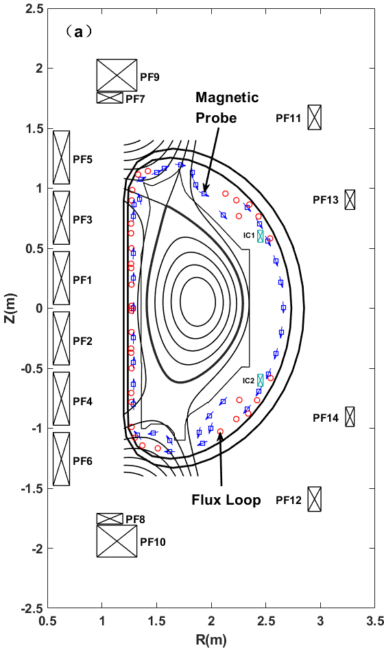
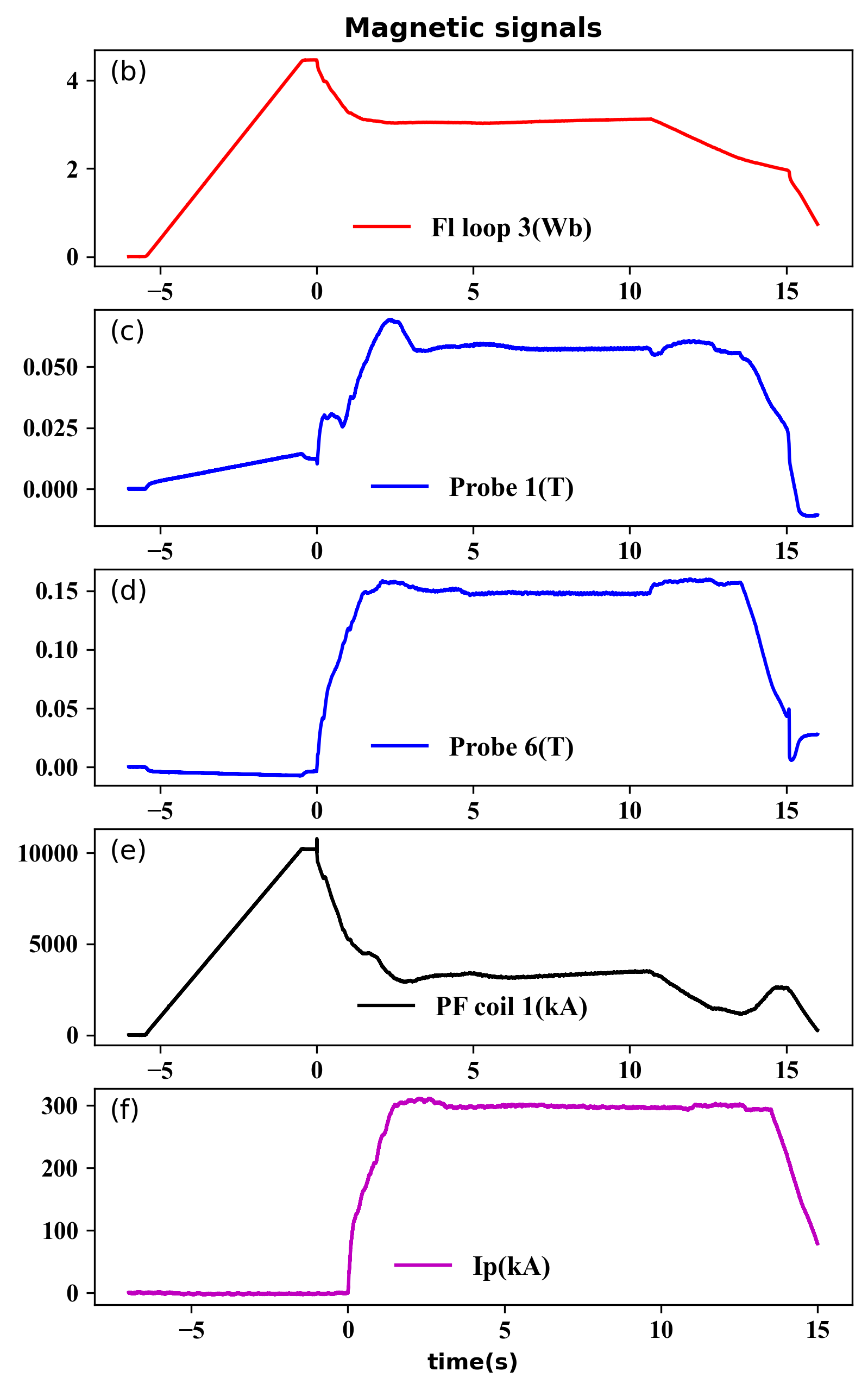
Figure 1:  Left: location of the magnetic probes, flux loops, and poloidal coils on EAST. A typical time evolution of some of the magnetic measurements from EAST discharge 113019 are plotted in the right panel. There are total 38 magnetic probes measuring the equilibrium poloidal magnetic field, and only 34 of them are working and are used in this work.

The inputs (features) to the neutral network (NN) are 84 magnetic measurements: 35 poloidal magnetic flux ($\Psi_{\operatorname{FL}}$) values measured by flux loops, 34 equilibrium poloidal magnetic field (MP) values measured by magnetic probes, 14 poloidal field (PF) coil currents and 1 plasma current (I_p) measured by a Rogowski loop.

The outputs (targets) of the neutral network are the values of the poloidal magnetic flux $\Psi$ at $R\times Z=129\times 129=16641$ spatial locations. The $\Psi$ used in the training process is computed by off-line EFIT and are downloaded from EAST MDSplus server (mds.ipp.ac.cn). The input and the output signals are interpolated to the same time slices before they are fed to the NN.

The inputs and outputs are summarized in Table 1.

Signal	Measure method	Signal meaning	Num. of values
Input			84
$\Psi_{\operatorname{FL}}$	Flux loop	Poloidal magnetic flux	35
MP	Magnetic probe	Poloidal magnetic field	34
PF	Rogowski loop	Poloidal field coil current	14
Ip	Rogowski loop	Plasma current	1
Output			16641
$\Psi$(R,Z)	EFIT	Poloidal magnetic flux	16641

Table 1:  The inputs and outputs of the model.

The data used in training, validation and testing process were downloaded from the EAST MDSplus server by using Python API, which scans a series of discharges and automatically skips discharges where necessary signals are missing. Specifically, we scan every 5 discharges among all the discharges spanning from #114000 to #117000, resulting in total 45,544 equilibria (time slices). These discharges are from experiments performed in one EAST campaign from June to July in 2022. This range is casually chosen with no particular criterion, except that we prefer recent discharges and avoid old discharges because locations of some magnetic probes were changed in previous campaigns. The auxiliary heating methods on EAST used in this campaign include neutral beam injection (50-70keV Deuterium beam), lower-hybrid waves (2.45GHz and 4.6GHz), electron cyclotron waves (140GHz), and ion cyclotron waves (25-70MHz). Typical values of total heating source power are between 4-10MW.

Figure 2 is the distribution of the EFIT equilibrium data in $(l_{i},\beta_{N})$ plane, where $l_{i}$ is the normalized internal induction and $\beta_{N}$ is the normalized plasma beta.

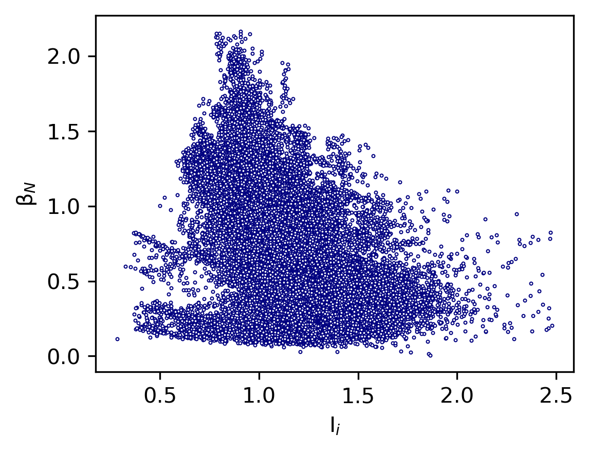
Figure 2: Distribution of the EFIT equilibrium data (training set + validation set+ testing set ) in $(l_{i},\beta_{N})$ plane.

The collected data are split into three sets: training set (81%), validation set (9%), and testing set (10%), where training set is used in training the NN, validation set is used in monitoring potential overfitting and tuning hyperparameters, and testing set is used in testing the predicting capability of the trained model.

Figure 1b-f shows that there is a difference of up to six orders of magnitude in the values of the input signals. In order to eliminate scale differences among features, we use the min-max normalization method to normalize the input data. The general formula is given by

$$x^{\prime}=\frac{x-x_{\min}}{x_{\max}-x_{\min}}$$ (3)

where $x$ is the original value of the feature, $x^{\prime}$ is the normalized value, $x_{\min}$ and $x_{\max}$ are respectively the minimal and maximal value of a feature in the data sets excluding the testing set. The $x_{\min}$ and $x_{\max}$ obtained here are then used to normalize the input data in the testing set when doing prediction using the trained NN.

Figure 3 plots the time evolution of the normalized input signals corresponding to those in Fig. 1b-f.

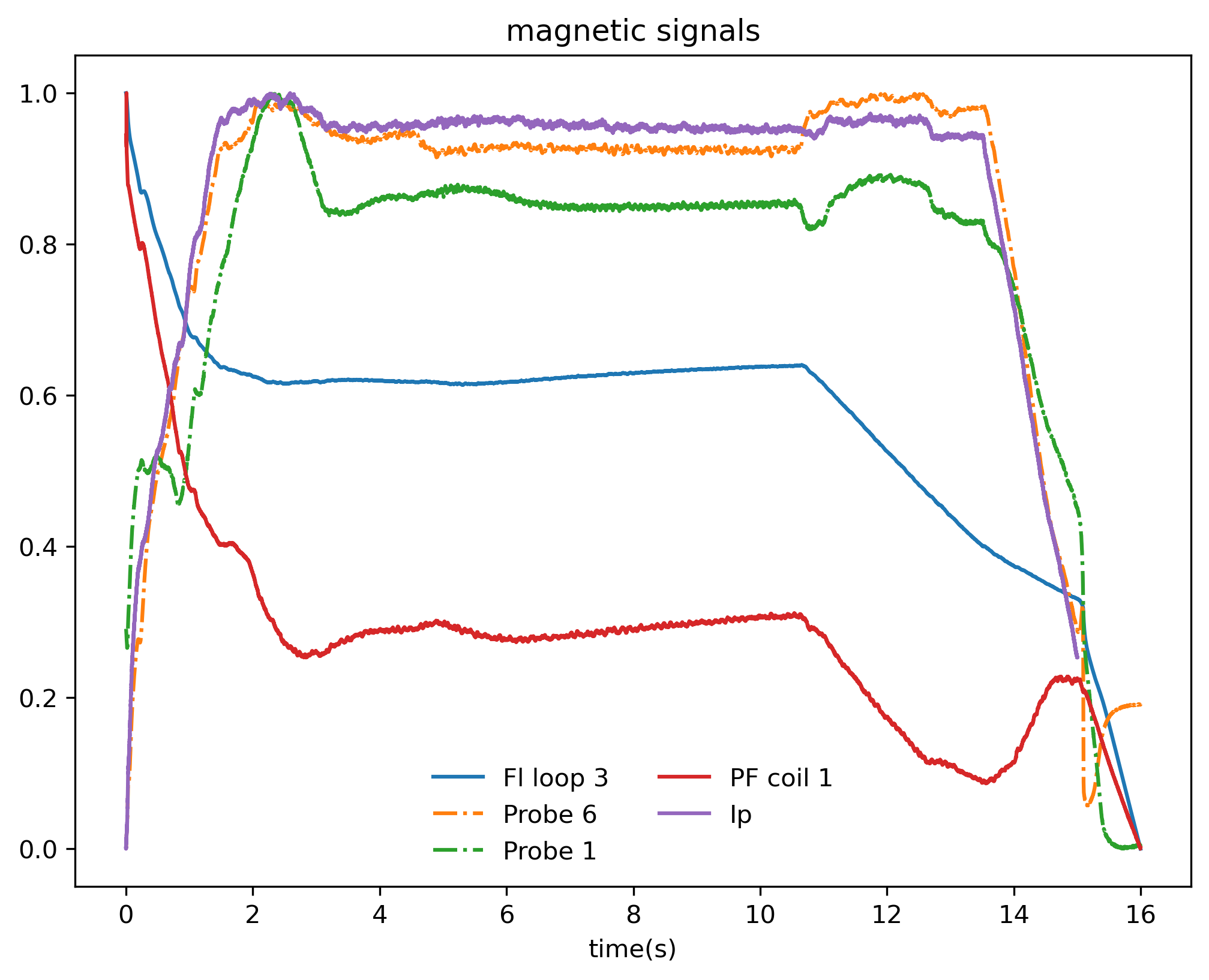
Figure 3: Normalized signals corresponding to those in Fig. 1b-f. The sudden change in the poloidal magnetic flux (Fl Loop 3) after 10s is brought about by the PF1 coil current, which is actively adjusted by the plasma control system to provide Ohm field to maintain a constant plasma current.

The magnitude of the output ($\Psi$ in SI units) is near 1, so no normalization is applied to it.

III Model architecture and automatic hyperparameter tuning

An artificial neural network is a kind of computational network, which usually consists of multiple layers: input layer, one or more inner layers (known as hidden layers), and a layer of outputs. Each layer is made of units. Each unit in the computing layers (hidden and output layers) receives information and process the information using some linear transform (matrix multiplication) and some nonlinear transform (activation function).

A fully-connected feed-forward network showed in figure 4 is used here to predict the poloidal magnetic flux $\Psi$ based on the magnetic measurements. Here “fully-connected” means that each unit of a computing layer receives information from all the units of the previous layer. “Feed-forward” means that information move in only one direction (from the input layer to the hidden layers, and to the output layers), no cycles or loops, and no intra-layer connections.

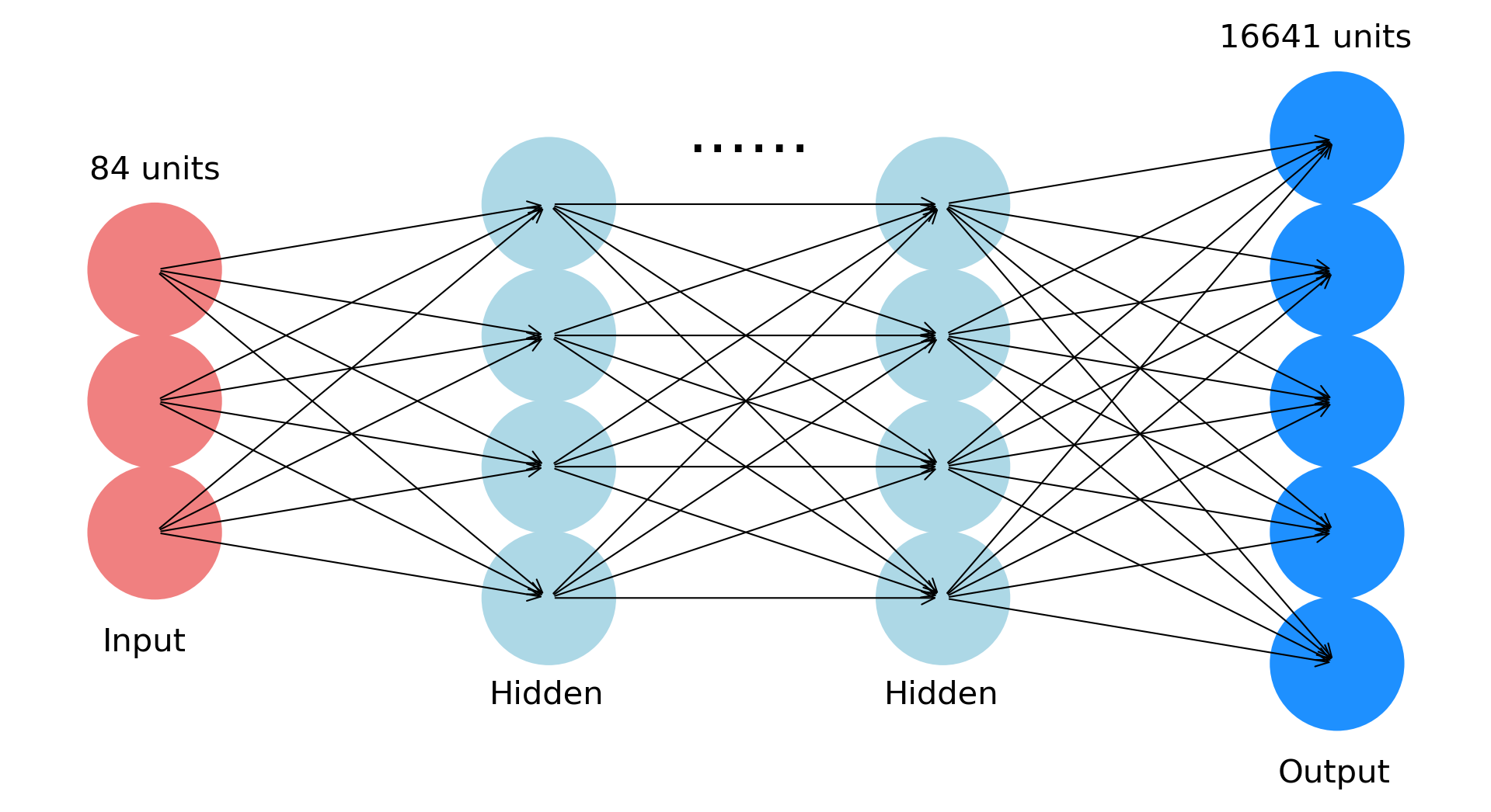
Figure 4: Fully connected feed-forward neural network used in this work.

Each unit (neuron or node) in the computing layers has trainable parameters, often called weights and biases. Denote the output of the $j^{\operatorname{th}}$ neuron in $l^{\operatorname{th}}$ layer by $a_{j}^{l}$, then a neural network model assumes that $a_{j}^{l}$ is related to the $a^{l-1}$ (output of the previous layer) via

$$a^{l}_{j}=\sigma\left(\sum_{k}w_{jk}^{l}a^{l-1}_{k}+b^{l}_{j}\right),$$ (4)

where $w^{l}_{jk}$ and $b_{j}^{l}$ are the weight and bias, the summation is over all neurons in the $(l-1)^{\operatorname{th}}$ layer, and $\sigma$ is a function called activation function. The weights and biases will be adjusted in the training process by gradient descent methods to reduce the loss (cost or error) function, which is defined in this work as

$$L(\mathbf{w},\mathbf{b})\equiv\frac{1}{2n}\sum_{i=1}^{n}\|\mathbf{y}_{i}-\hat{\mathbf{y}}_{i}\|^{2},$$ (5)

where $\mathbf{y}_{i}$ is the EFIT poloidal magnetic flux and $\hat{\mathbf{y}}_{i}$ is the NN output, and the summation is over all the samples in the training set. The loss function in Eq. (5) is the mean squared error (MSE). The loss function measures the derivation of the approximate solution away from the desired exact solution. So the goal of a learning algorithm is to find weights and biases that minimize the loss function. To minimize the loss function over $(\mathbf{w},\mathbf{b})$ using the gradient descent method, we need to compute the partial derivatives $\partial L/\partial w^{l}_{jk}$ and $\partial L/\partial b^{l}_{j}$, which can be efficiently computed by the well known back-propagating methodRumelhart1986 (15, 16). The back-propagating algorithm and the corresponding gradient descent method are the core algorithms in all deep learning software frameworks.

Besides the trainable parameters, there are various hyperparameters in a NN that usually need to be set manually, such as number of hidden layers, units per layer, activation function, NN optimizers, learning rate, batch size, number of epochs of training. In recent years, there appear automatic optimization libraries that can search for the best combination of hyperparameters. In this work, we use the Optuna optimization frameworkoptuna_2019 (14) in setting the hyperparameters. Optuna automates the hyperparameter optimization process by defining a search space of hyperparameters and exploring the space using efficient searching algorithms. The tree-structured Parzen estimator (TPE) algorithm is used in this work. This algorithm models the relationship between hyperparameters and their corresponding performance metrics and makes efficient decisions on which hyperparameters to try next.

Optuna automate the selection of the best hyperparameter combination. After multiple experiments, we have found that the model accuracy is not sensitive to the number of hidden layers, activation functions, and optimizers (an example showing the relative importance of these hyperparameters is given in Fig. 5). Therefore, these hyperparameters are fixed in the fine tuning step, in order to improve the speed of the model selection process, and explore more hyperparameter regimes to which the model may be sensitive. For other hyperparameters, we use Optuna framework to find the optimal combination of hyperparameters. Relative importance of these hyperparameters are shown in Fig. 6. The above results indicate that learning rate is the dominant factor that determines the model performance.

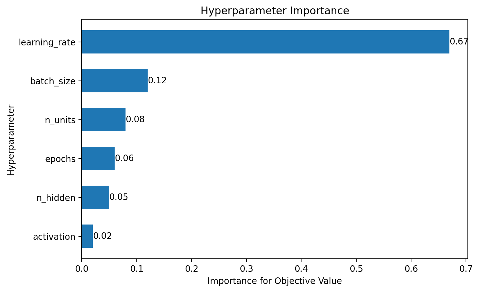
Figure 5: Hyperparameter importance distribution. Model accuracy is not sensitive to activation functions for this case.

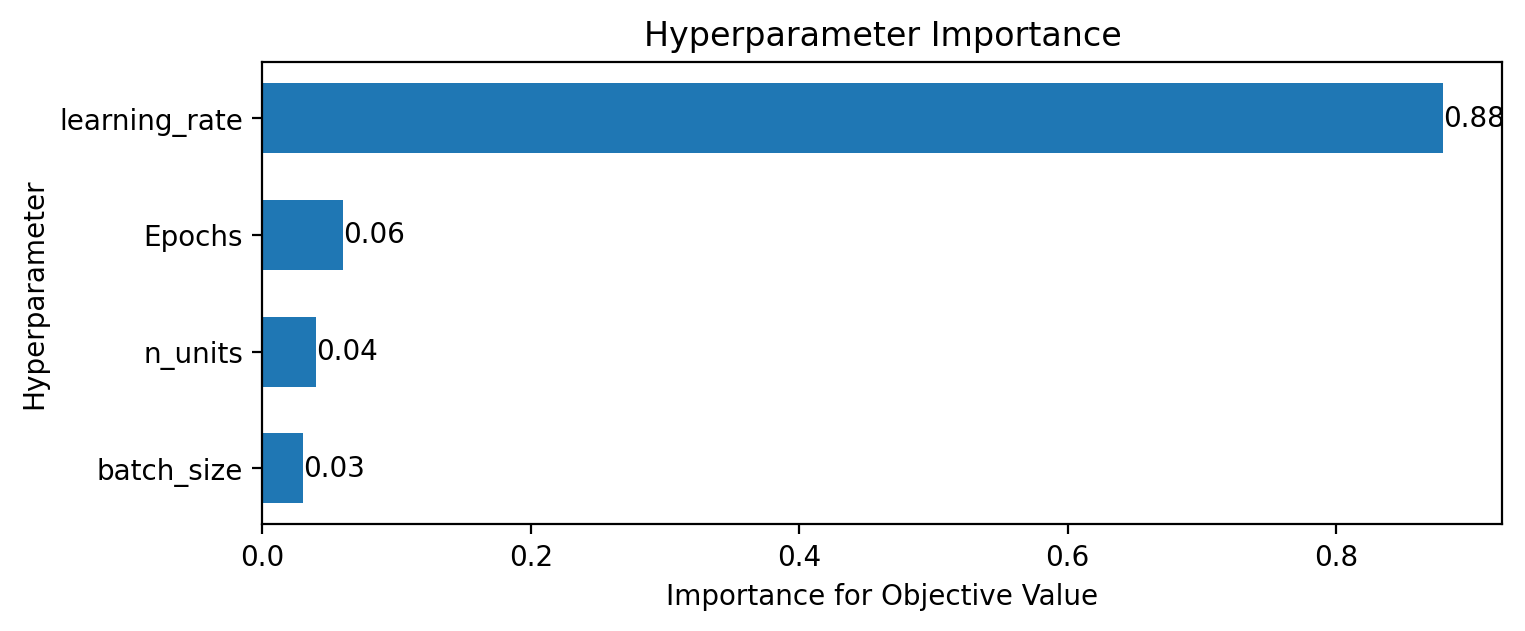
Figure 6:  Relative importance of the hyperparameters in determining the model accuracy in the fine tuning.

The final values of the hyperparameters used in the model are shown in Table 2.

Hyperparameter	Meaning	Final values
n_layers*	Number of hidden layers	4
n_units	Number of nodes per hidden layer	86
Activation*	Activation function	tanh
Optimizer*	Optimizer type	Adam
$\eta$	Learning rate	$2.26\times 10^{-5}$
Loss*	Loss function	MSE
batch_size	Number of samples used in a step	16
Epochs	Number of epochs	97

* Fixed hyperparameters during fine tuning

Table 2:  Final values of hyperparameters of the model. The hyperparameters with an asterisk (*) are fixed during the fine tuning. The above activation function refers to that used in the hidden layers. For the output layer, the linear activation function is used.

The network are constructed and trained using Keras & TensorFlow2 chollet2015keras (17, 18), which is a broadly adopted open source deep learning framework in industry and research community. Figure. 7 plots loss function values as a function of the training epochs. The loss function is also evaluated on the validation set, which serves as a monitor for the possible overfitting. The validation loss follows the same trend as the training loss, indicating no overfitting.

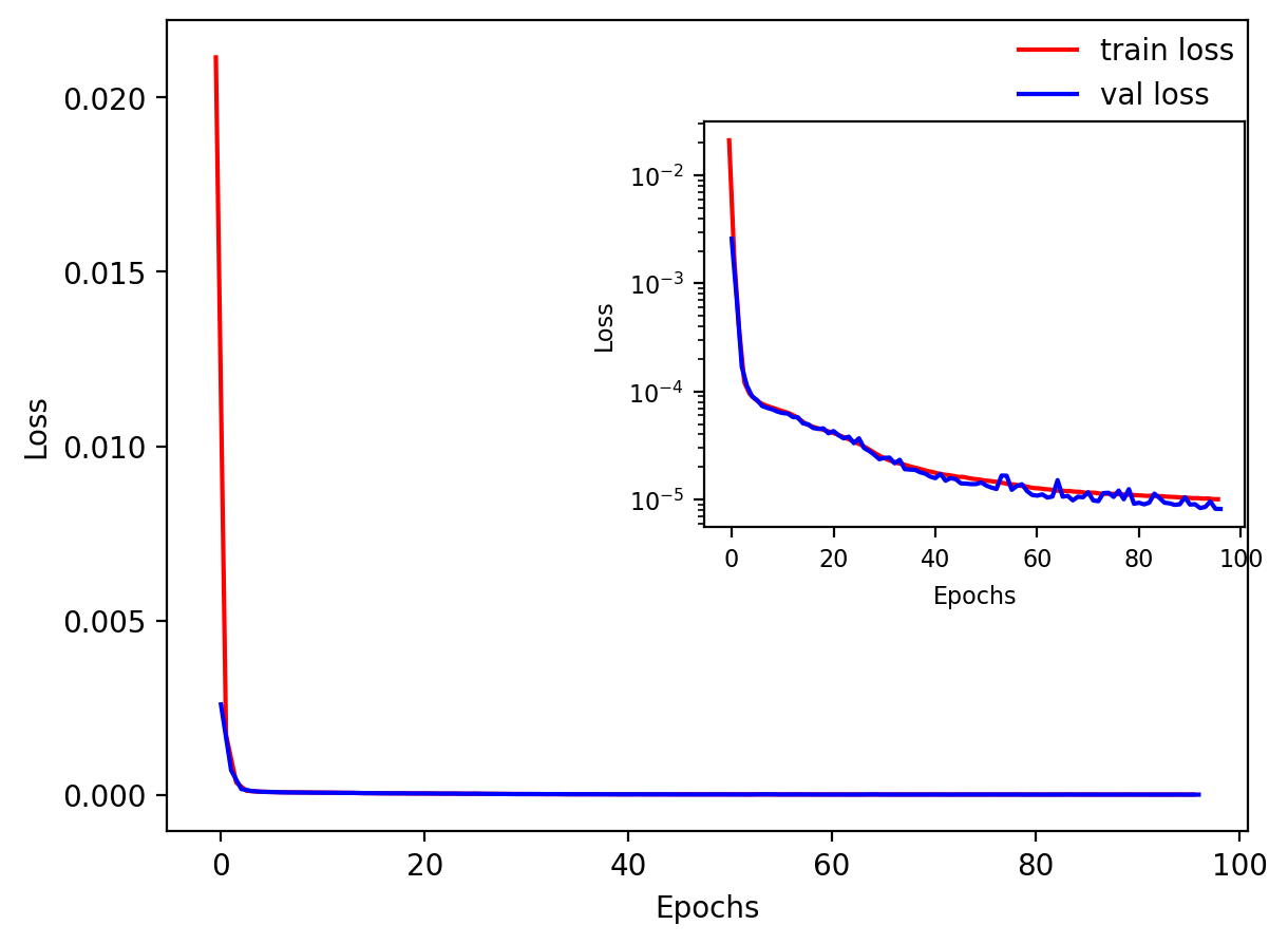
Figure 7: Training history showing the training and validation loss function values versus the training epochs. One epoch corresponds to go through all the samples in the training set. In the mini-batch stochastic gradient descent method used here, each gradient descent step uses randomly selected 16 samples (a mini batch), and the loss function values shown here are obtained by summation over a mini batch of samples in the training set or validation set.

IV Performance of the neural network

IV.1 Performance of the model on testing set

After the model is trained on the training set, we assess its prediction capability on the data that are not seen by the training process. To evaluate the reconstruction quality, we employ three widely adopted metrics: the Pearson correlation coefficient $r$ (definition is given in appendix A), the coefficient of determination $R^{2}$ (definition is given in appendix B), and the peak signal-to-noise ratio (PSNR) (definition is given in appendix C).

Figure 8a plots the NN prediction of the poloidal flux $\Psi_{NN}$ vs. EFIT results $\Psi_{\operatorname{EFIT}}$ for the testing set (total 4555 equilibria, each with 16641 values). The Pearson correlation coefficient $r$ and the coefficient of determination $R^{2}$ are also shown in the figure, which are very close to 1, indicating a strong predictive capability. Figure 8b plots the distribution of the correlation coefficient $r$ between NN predictions and EFIT results for each equilibrium of the 4555 equilibria in the testing set. The results indicate that the majority of the values are greater than 0.998, indicating good correlation between NN prediction and EFIT result for each equilibrium.

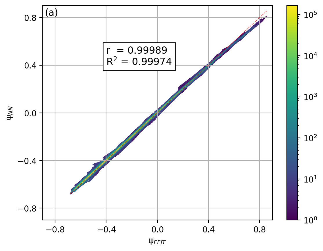
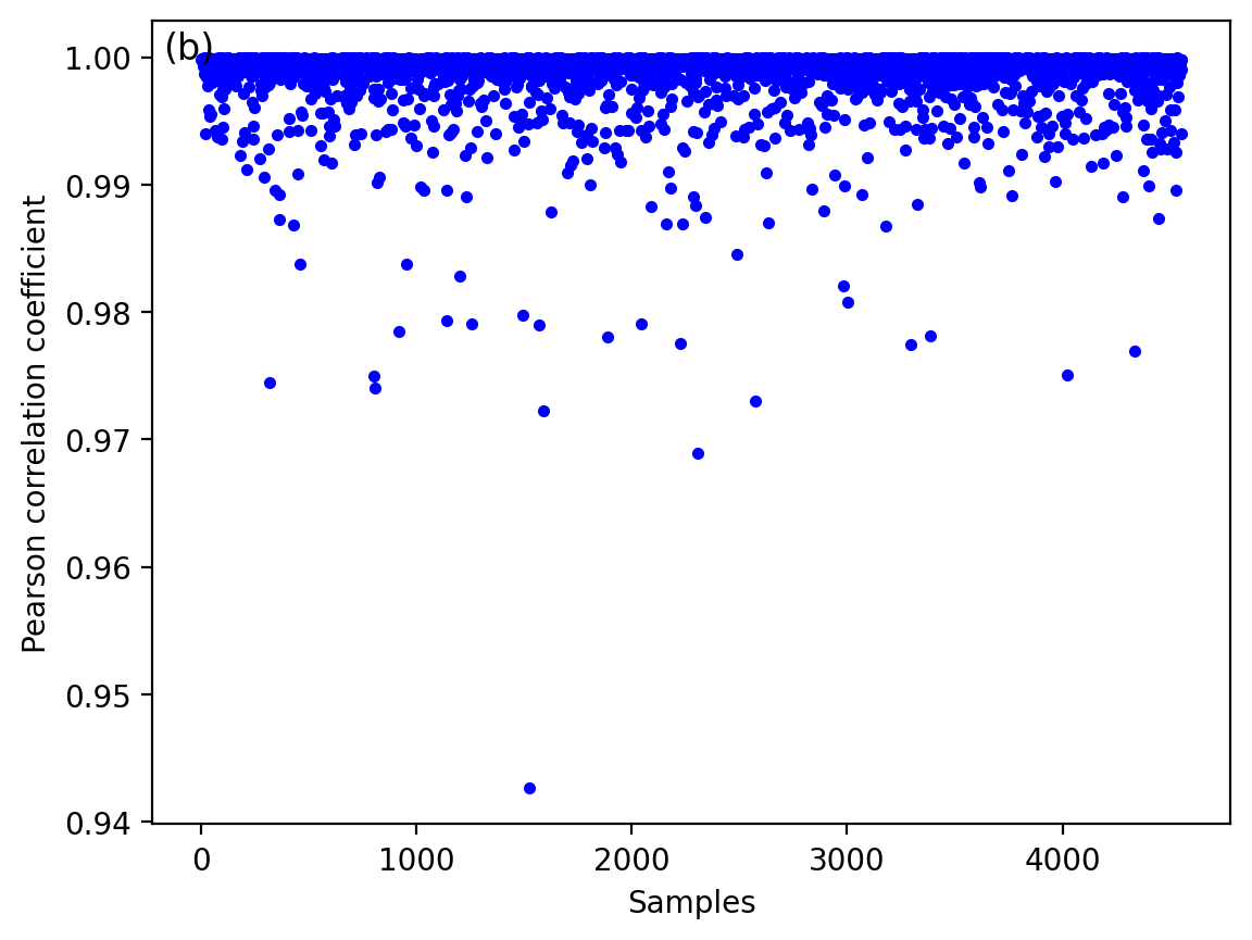
Figure 8: (a) Neural network prediction of the poloidal flux $\Psi_{NN}$ vs. EFIT results $\Psi_{\operatorname{EFIT}}$ for the testing set (total 4555 equilibria). Red dashed line is the $y=x$ line. The total number of points shown here is $4555\times 129\times 129$. Color represents density of data points. (b) The distribution of the correlation coefficient for each equilibrium of the 4555 equilibria in the testing set.

To test the accuracy of the model in predicting the plasma magnetic surface, we compare the 2D contours of the poloidal magnetic flux predicted by the NN with those given by EFIT. The results are shown in figures 9(a), (c), (e) and (g), where the NN predictions of $\Psi$ contours are overlaid on the $\Psi$ contours of EFIT. It displays four randomly selected samples from the 4555 equilibria in the testing set (the four displayed samples may not necessarily come from the same discharge). Since our reconstruction results take the form of images with resolution determined by the spatial grid points, it is also useful to use $\operatorname{PSNR}$ in evaluating the reconstruction quality of the magnetic surface. The values of PSNR for the four equilibrium are shown in the figure.

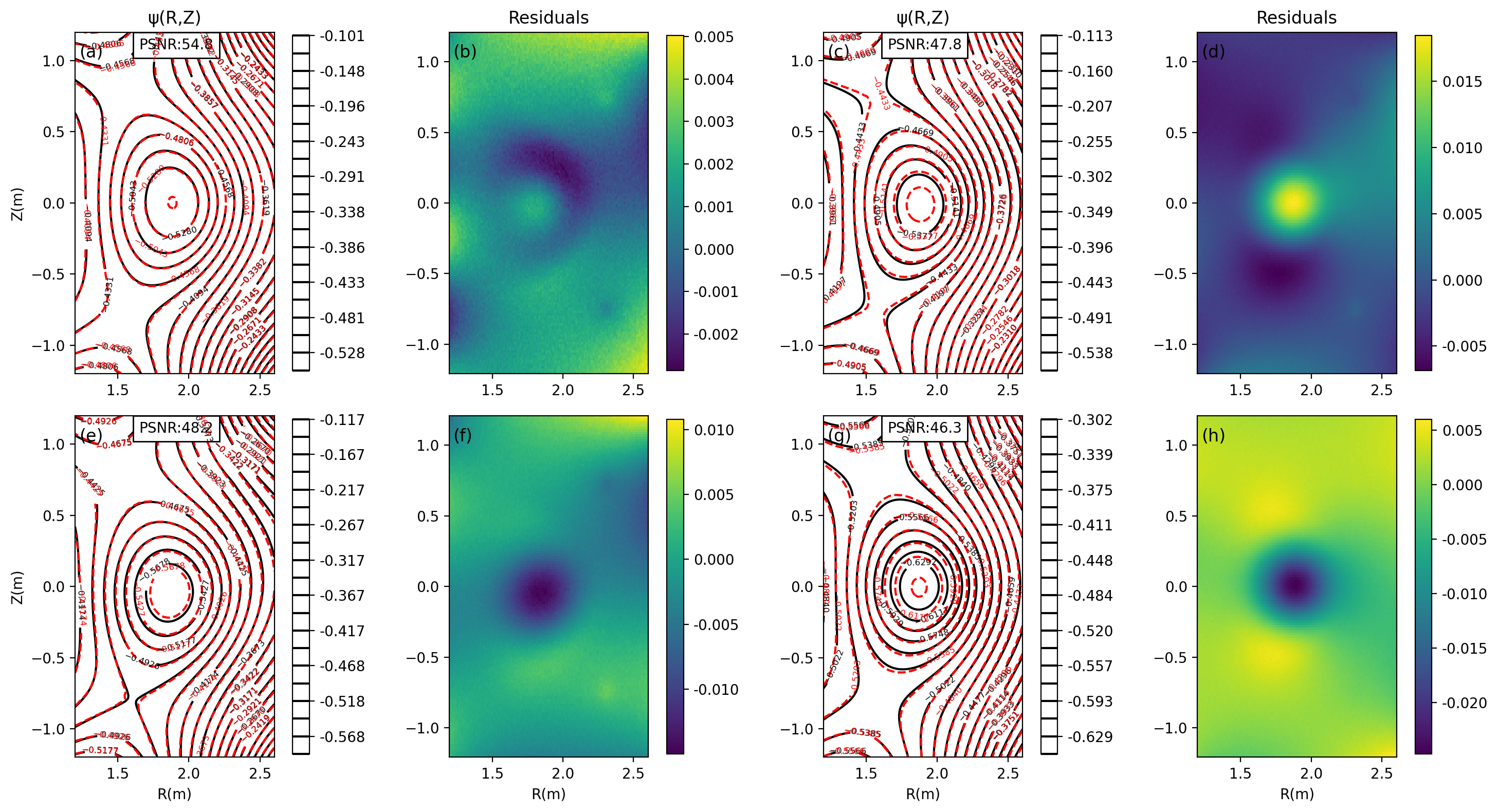
Figure 9: Panels (a), (c), (e) and (g) compare the magnetic surfaces from EFIT (solid black lines) with those from the NN (dashed red lines) for four randomly selected time slices from the 4555 testing samples. Panels (b), (d,) (f) and (h) show the corresponding normalized residua [$\Psi$(R,Z) $\Psi^{\operatorname{NN}}$(R,Z)]/max(|$\Psi$ (R,Z)|).

To further assess the accuracy of the mode, we locate the LCFSs predicted by the NN model and compare them with those given by EFIT. The LCFSs corresponding to the four equilibrium of Fig. 9 are shown in Fig. 10, which indicates that the NN and EFIT results are in good agreement. Minor discrepancies appear near the X points.

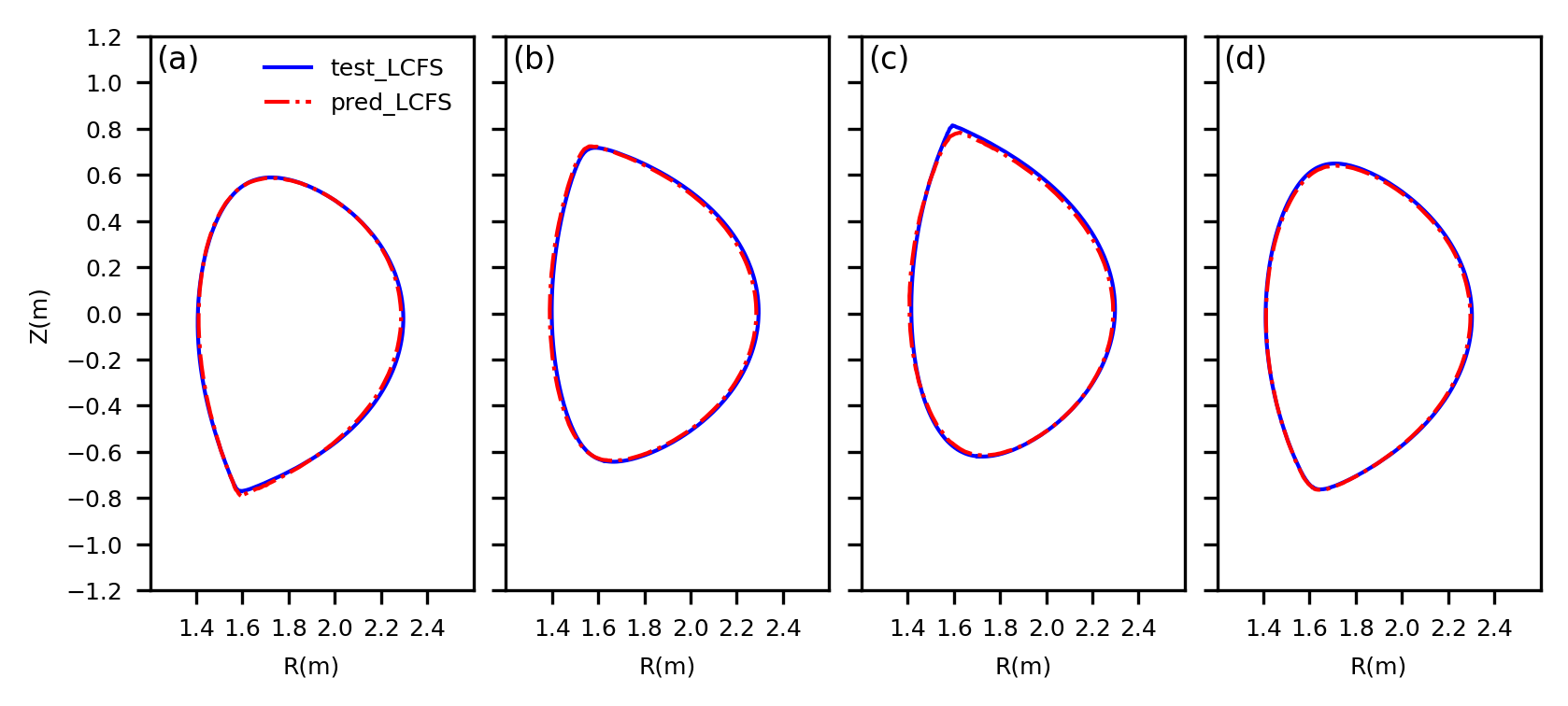
Figure 10: Comparison of LCFS between the NN prediction and EFIT result. The four panel correspond to the four equilibria shown in fig. 9. In locating the LCFS from the NN prediction, we analyze a series of $\Psi$ contours and determine the outermost contour that are near the magnetic separatrix.

IV.2 Performance of the model on four complete discharges

In this section, we arbitrarily select 3 full discharges that are not in the dataset used above to examine the time evolution of the magnetic configuration during an entire discharge (from ramp-up to flat-top then to ramp-down).

Besides the plasma currents $I_{p}$, we also calculate the normalized internal inductance $l_{i}$ (definition is given in Appendix D), which is a quantity that is solely determined by $\Psi$ and thus can further reflect how accuracy the predicted $\Psi$ is. We plot the time evolution of $l_{i}$ and compare it with the EFIT results. By doing this, we can assess the accuracy of the NN in predicting the time evolution of some key volume-integrated quantities characterizing magnetic configuration.

Figure 11 compares the time evolution of $I_{p}$ and $l_{i}$ predicted by the NN and that by EFIT for discharge #113388.

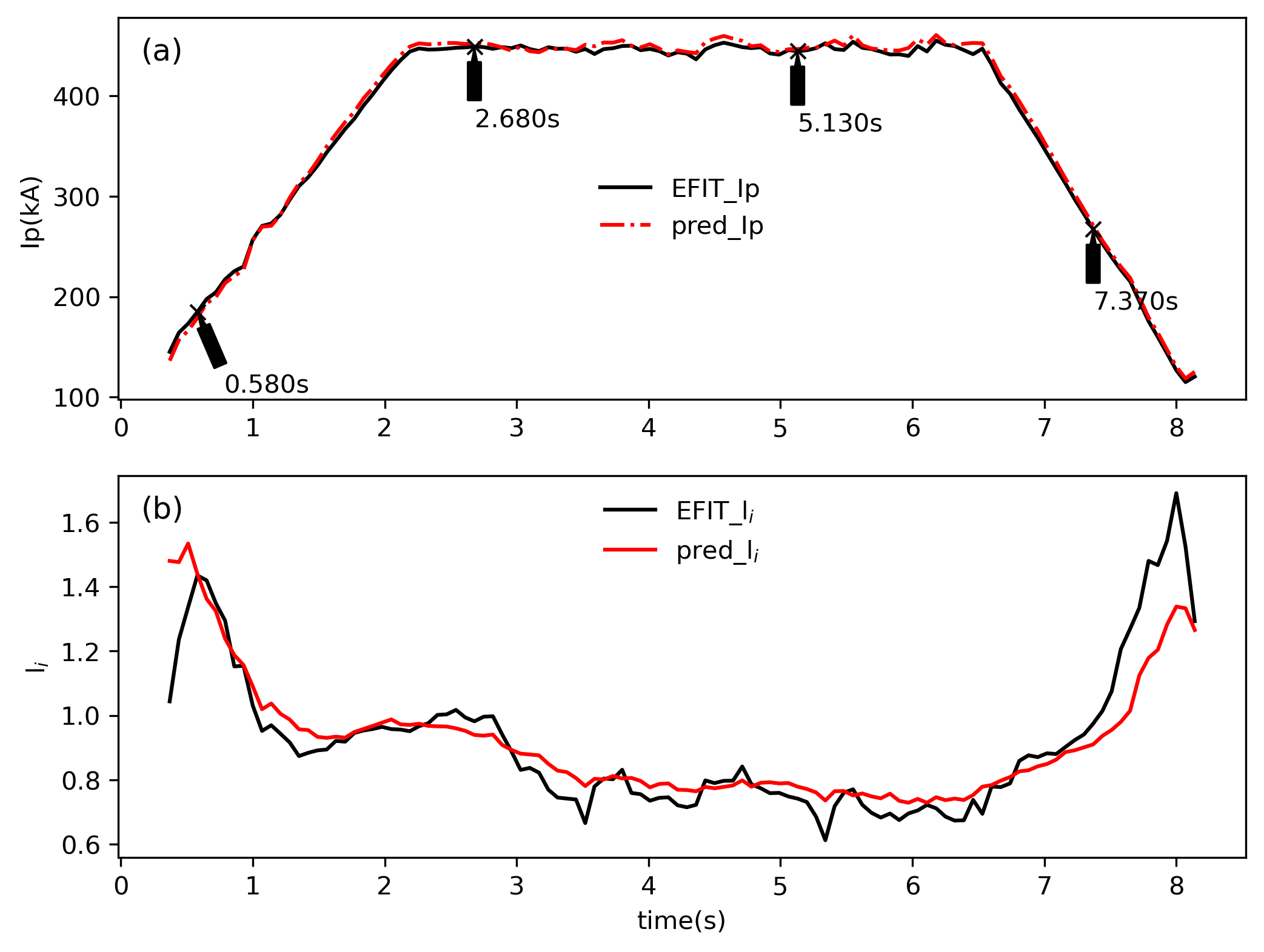
Figure 11: (a) Comparison of time evolution of plasma current given by the NN and EFIT. (b) Comparison of time evolution of $l_{i}$ given by the NN and EFIT. Four time slices are indicated on the graph, which are time slices selected for the magnetic configuration comparison shown in Figs. 12-13.

Figure 12 compares the contours of $\Psi$ given by the NN model and that given by EFIT at 4 time slices (indicated in Fig. 11) in discharge #113388. The results indicate the relative error between the NN and EFIT results is less than $2\%$.

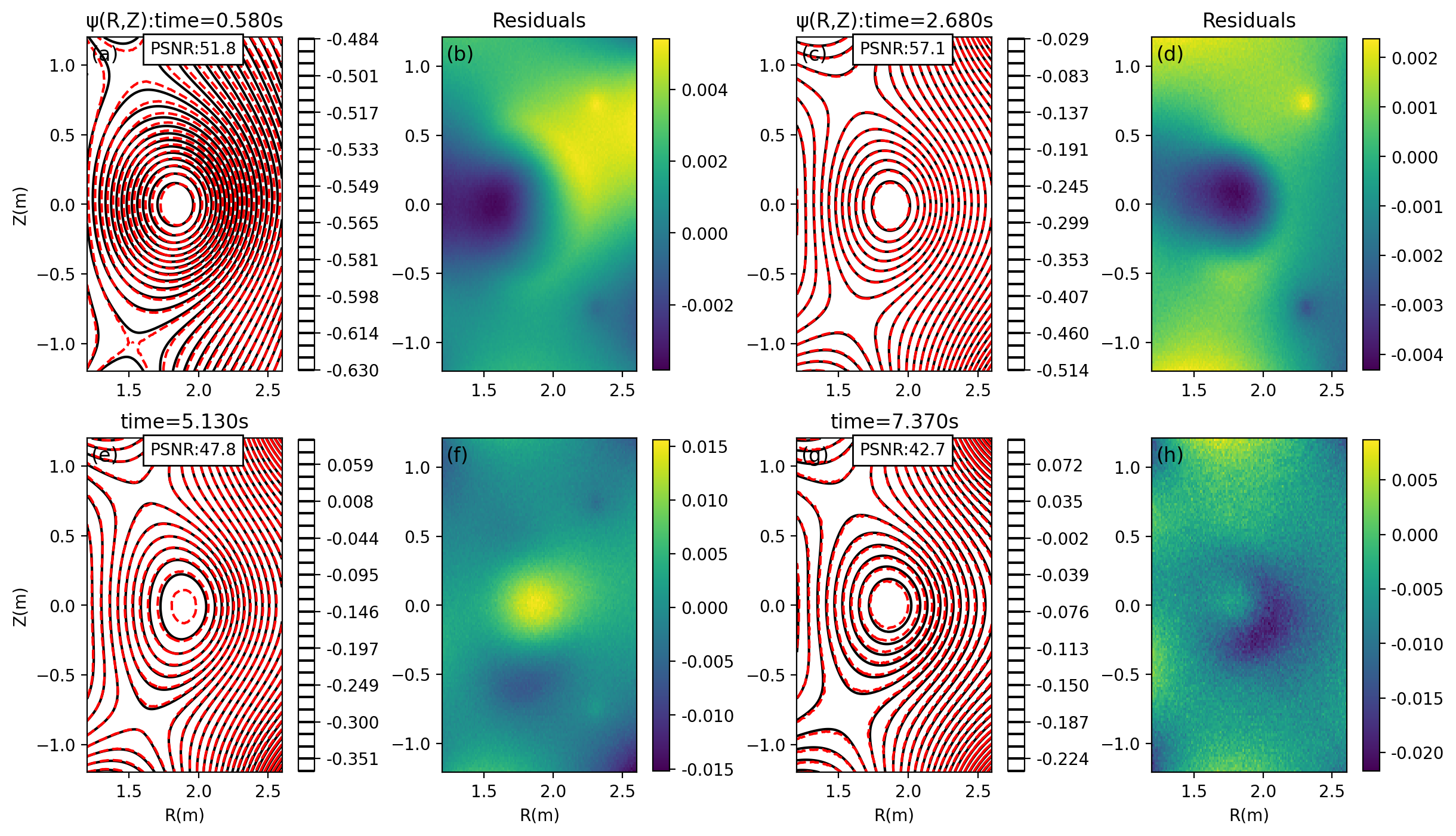
Figure 12: Panels (a), (c), (e) and (g) compare the magnetic surfaces from EFIT (solid black lines) with those from the NN (dashed red lines) for discharge #113388. $\Psi$ at four different time slices during the discharge, 0.580s (early ramp-up), 2.680s,, 5.130s (flat top), 7.370s (ramp-down)  are shown. Panels (b), (d,) (f) and (h) show the corresponding relative error  $(\Psi_{\operatorname{EFIT}}-\Psi_{\operatorname{NN}})/\max(|\Psi_{\operatorname{EFIT}}|)$.

Figure 13 compares the LCFSs given by the NN model and that given by EFIT at 4 time slices in discharge #113388. The results show good agreement between the two models. Minor differences usually appear in the ramp up/down phase, and near the X-points.

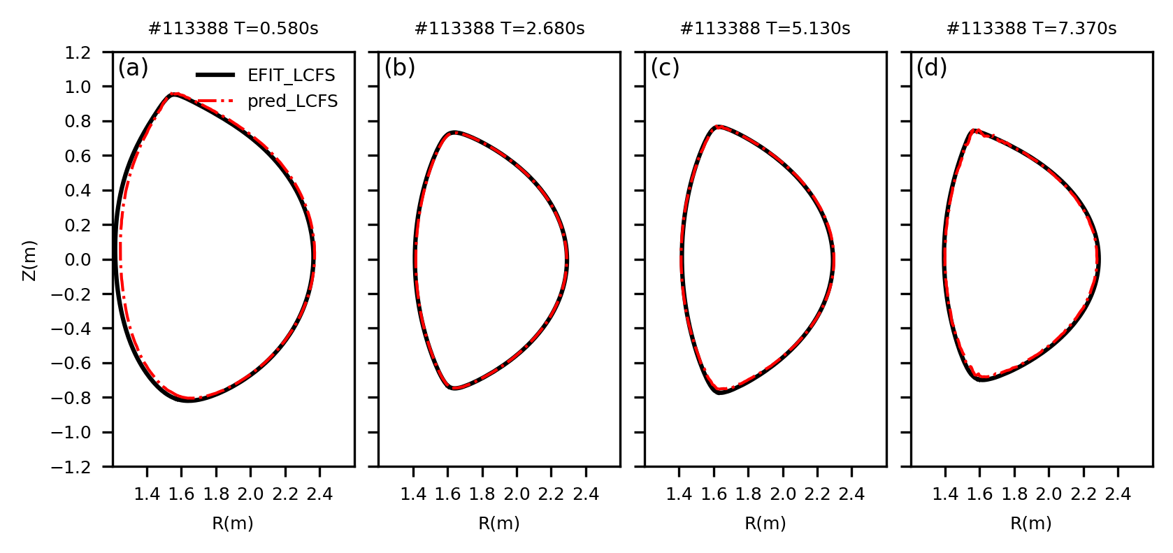
Figure 13: NN reconstructions of the LCFS (dotted-dashed red) for EAST shot #113388 overlaid against the EFIT LCFS (solid black). LCFSs from four different times in the discharge #113388 are shown.

Similar results for discharge  #117016 are shown in Fig. 14-16.

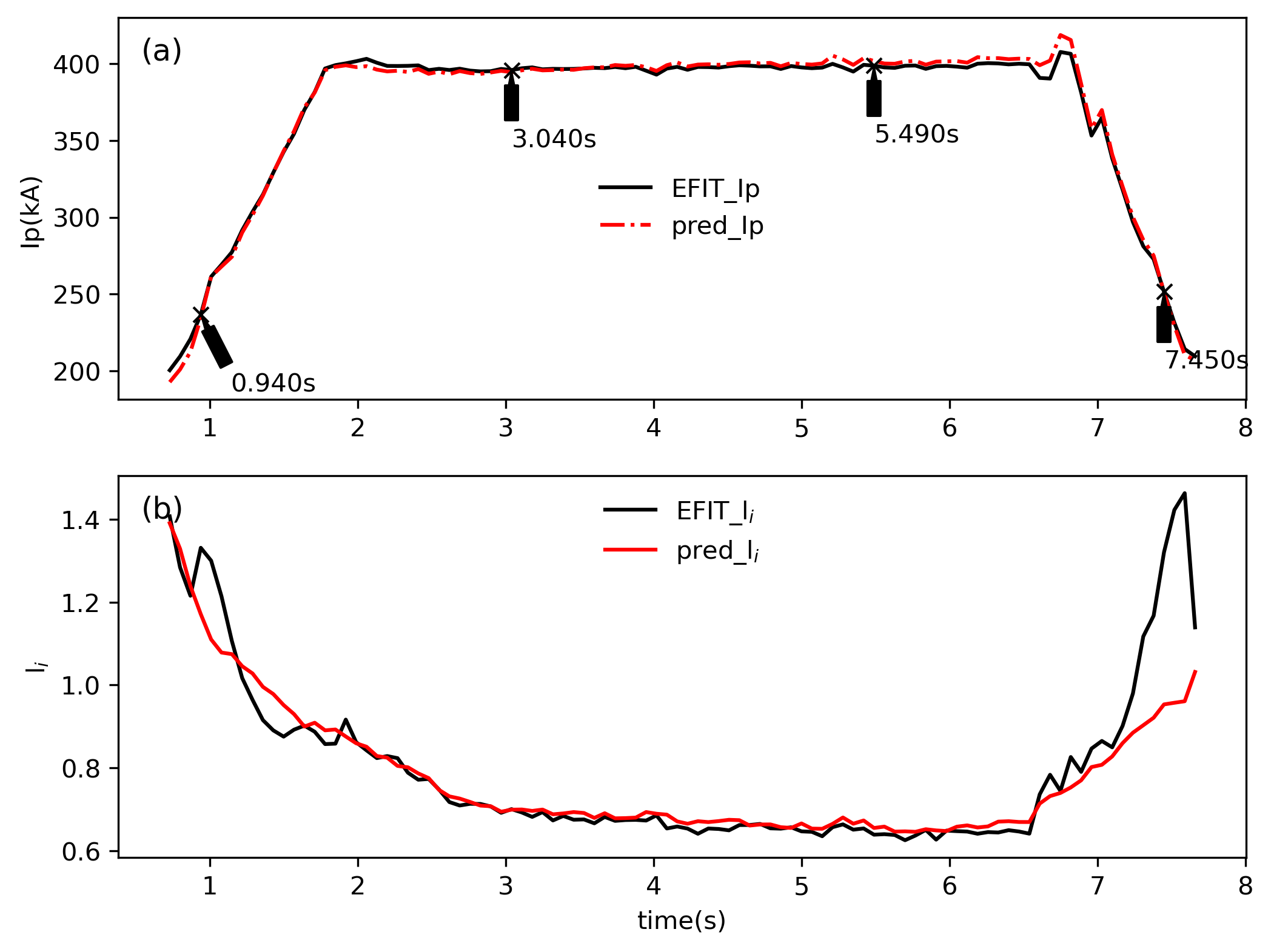
Figure 14: Same as figure 11, except that the discharge is #117016.

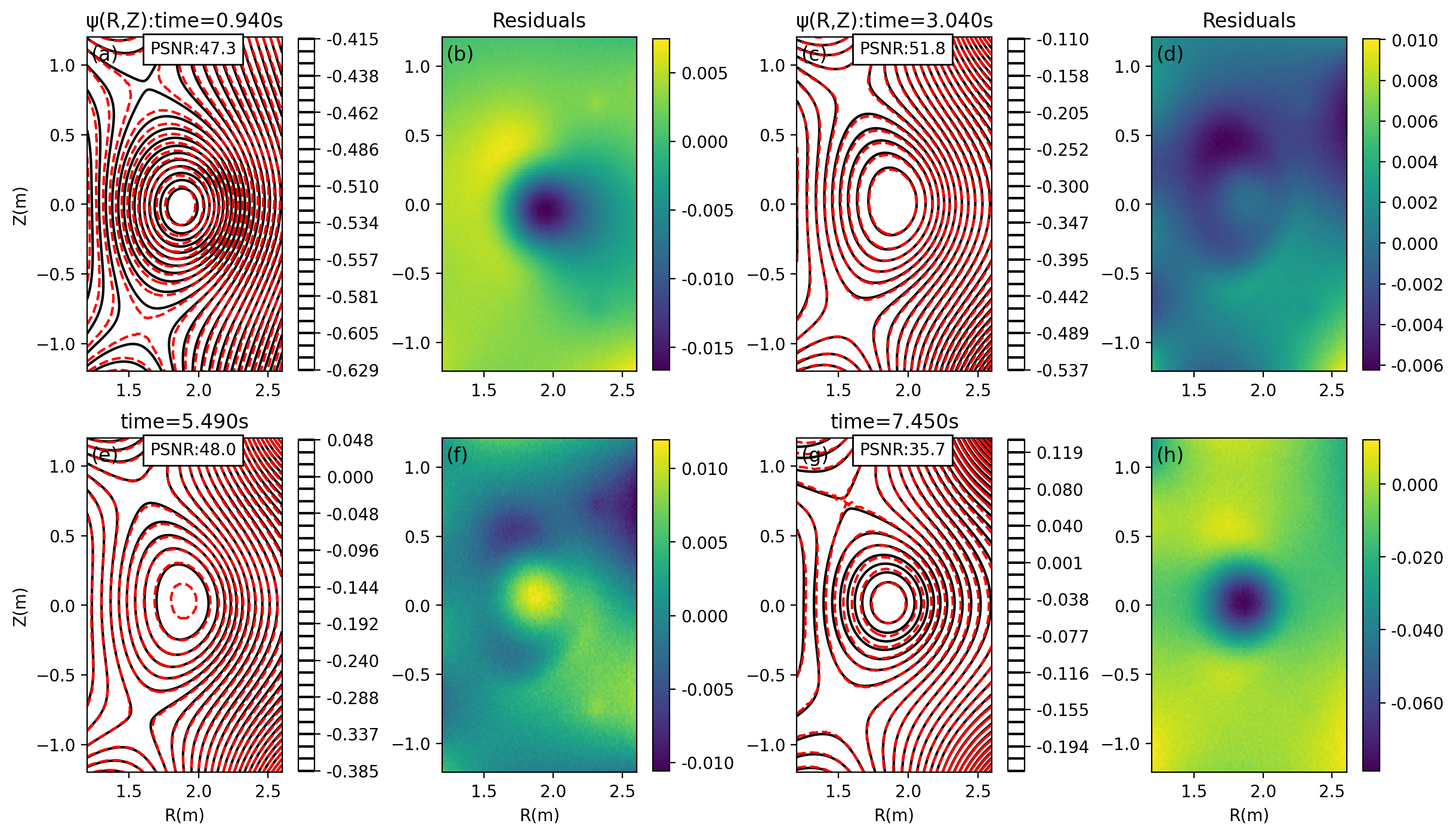
Figure 15: Same as figure 12, except that the discharge is #117016.

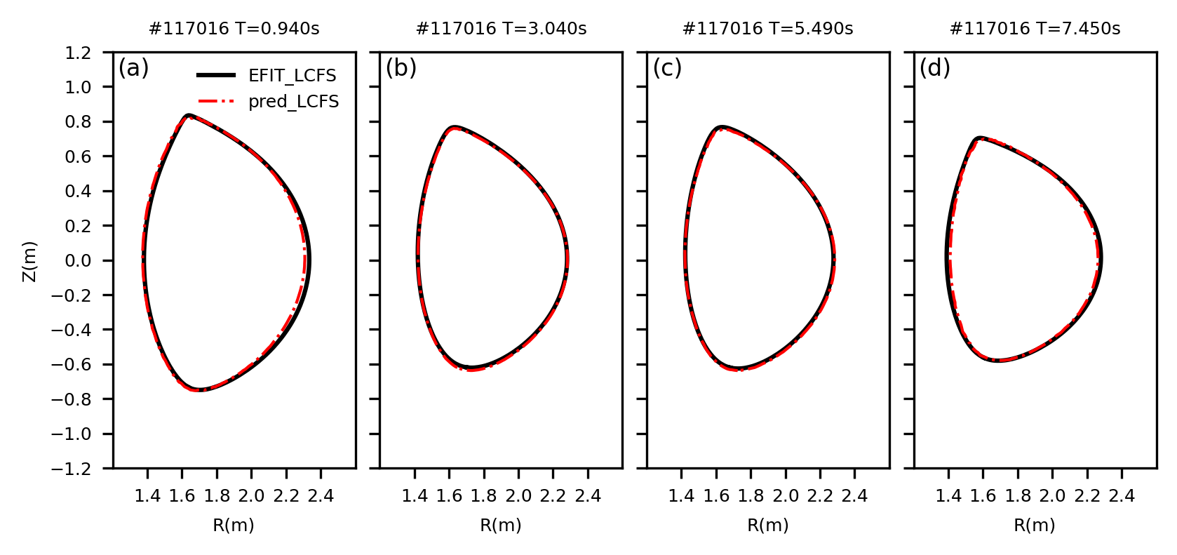
Figure 16: Same as figure 13, except that the discharge is #117016.

Similar results for discharge  #113019 are shown in Fig. 17-19.

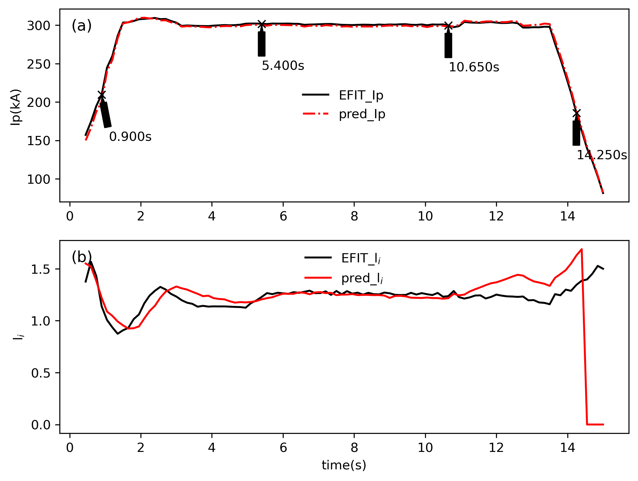
Figure 17: Same as figure 11, except that the discharge is #113019.

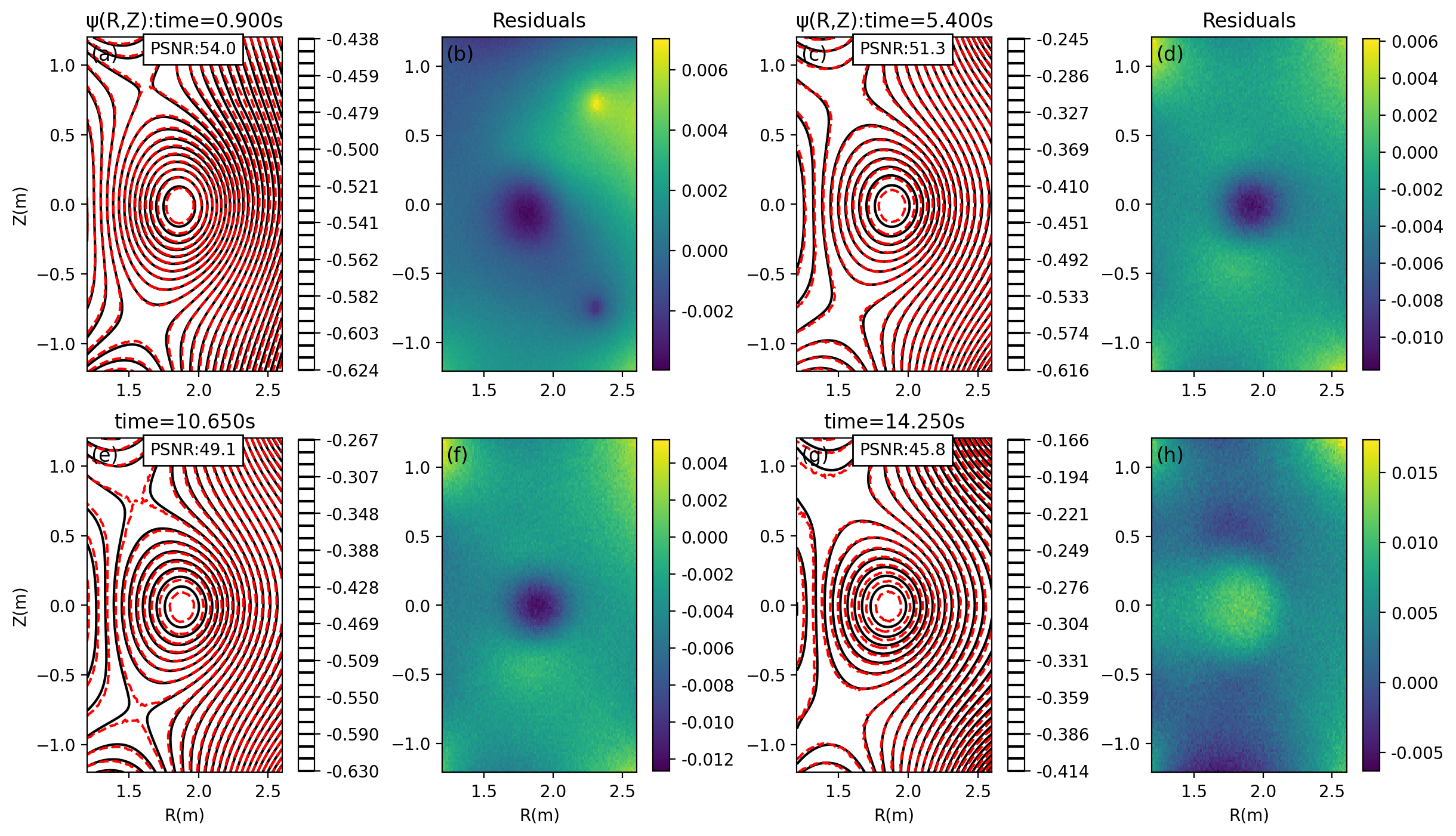
Figure 18: Same as figure 12, except that the discharge is #113019.

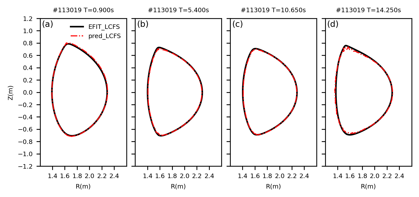
Figure 19: Same as figure 13, except that the discharge is #113019.

V Neural network prediction of $W_{\operatorname{mhd}}$, $\beta_{N}$, and $q_{95}$

Besides the $l_{i}$ discussed above, there are some other global parameters that can be constructed from the magnetic measurements, namely the plasma stored energy $W_{\operatorname{mhd}}$, normalized plasma beta $\beta_{N}$, and edge safety factor $q_{95}$. These parameters depend on information beyond the poloidal magnetic flux, namely the toroidal magnetic field and plasma pressure. Therefore they can not be fully determined by using only the poloidal magnetic flux predicted from the above network.  Following Ref. DIII-D_2022 (8), we construct a new NN for predicting these parameters (called NN2 in the following; the previous one will be called NN1), where the network has only 3 output values, namely $W_{\operatorname{mhd}}$, $\beta_{N}$, $q_{95}$. The input to NN2 includes a new signal, the current in the toroidal field (TF) coils, which determines the toroidal field. (In the NN1, this signal is not included because it has negligible effect on the prediction of the poloidal magnetic flux.) The NN2 has only one hidden layer consisting of 16 units, and uses the sigmoid as the activation function for both the hidden and output layers. The input and output signals of NN2 are normalized by using the same min-max scalar as used for NN1.

The training data consist of about $1/4$ randomly selected part of the data used for NN1. We found that using larger dataset makes this small network prone to overfitting. The testing set consists of 1000 time slices. Figure 20 plots the NN2 predictions against the EFIT values for the testing set. The results indicate that the NN2 predictions are in reasonable agreement with the EFIT values for all the 3 parameters. The NN2 predictions of $q_{95}$ are a little worse than those of the other two parameters, judging from the values of $r$ and $R^{2}$.

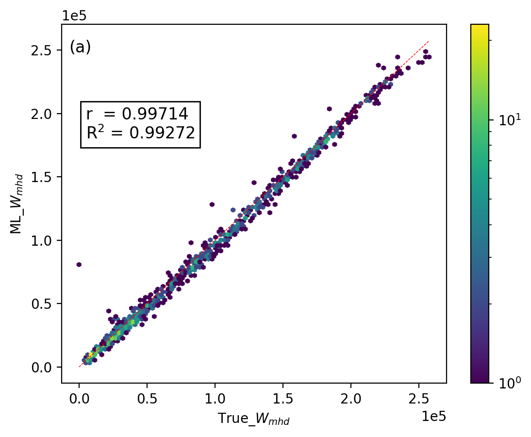
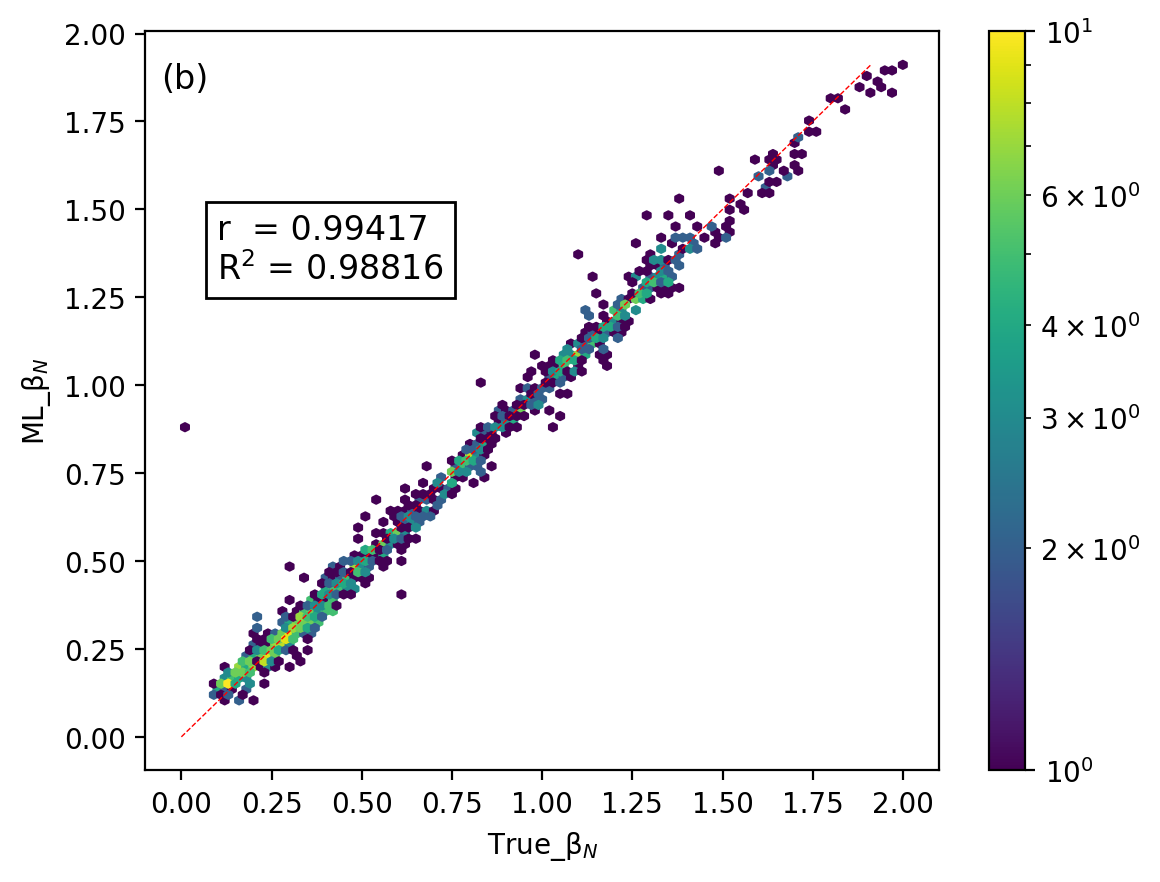
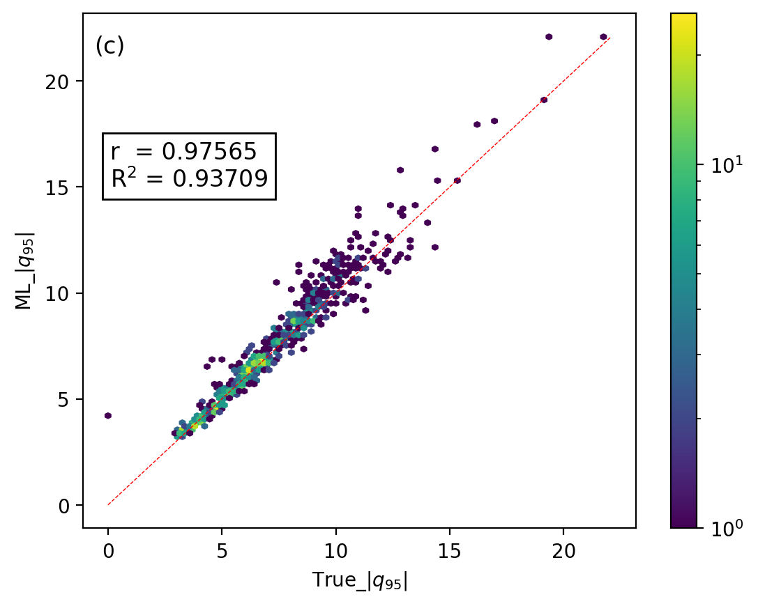
Figure 20: NN2 predictions of $W_{\operatorname{mhd}}$, $\beta_{N}$, and $q_{95}$ against the EFIT values for the testing set.

To evaluate the accuracy of NN2 prediction for a full discharge, we arbitrarily chosen a discharge and compare the time evolution of $W_{\operatorname{mhd}}$, $\beta_{N}$, and $q_{95}$ between the NN2 predictions and EFIT values. The results are shown in Fig. 21, which shows good agreement between the network predictions and EFIT values.

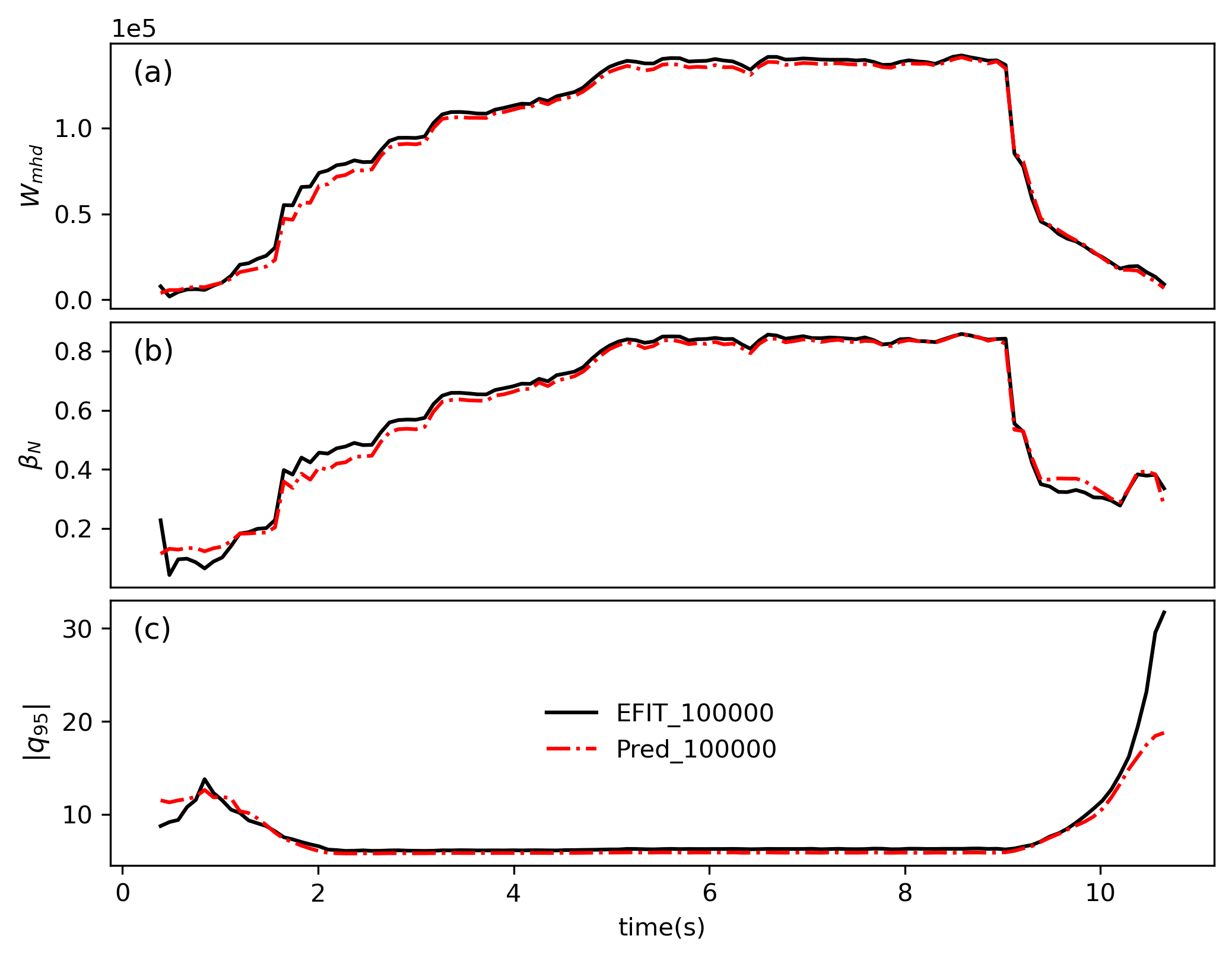
Figure 21: Time evolution of plasma stored energy $W_{\operatorname{mhd}}(J)$, normalized beta $\beta_{N}$, and edge safety factor $q_{95}$ in EAST discharge #100000. Solid lines are EFIT values and dash-dot lines are network predictions.

VI Summary and discussion

In this work, we train a multiply-layer neural network on the magnetic measurements (input) and EFIT poloidal magnetic flux (output) on EAST tokamak. The prediction capability of the network is examined by comparing the reconstructed magnetic surfaces, last closed flux surfaces, plasma current, and normalized internal inductance with those of EFIT. The neural network shows good agreement with EFIT for the data unseen in the training process.

In constructing the neural network, we use automatic optimization in searching for the best hyperparameters of the model. The hyperparameters found this way turn out to be better than our previously manually set hyperparameters in terms of the model accuracy.

Based on the model’s good prediction capability and efficiency in terms of computational time (about 0.5ms per equilibrium on a desktop computer, using an 11th Gen Intel(R) Core(TM) i5-11500@2.70GHz CPU with a single thread), it looks promising to apply the neural network to real-time magnetic configuration control. The above computational time does not include the time used for tracing boundary/internal magnetic surfaces, and other related calculations to obtain $l_{i}$. These computations (not optimized in this work) seem too inefficient to be used in real-time control. The purpose of computing $l_{i}$ for the NN1 model is to evaluate the accuracy of the predicted $\Psi$. To predict these volume-integrated parameters, one usually uses an additional small network, as we did in Sec. V, which is efficient enough for real-time control because the network size is usually very small.

This work is limited to magnetic measurements. We plan to add more diagnostics relating to the inner safety factor profiles and pressure profiles into the model, in order to construct more realistic equilibria. This will rely on the kinetic EFIT output. We are accumulating these kind of training data.

VII Data availability

The data that supports the findings of this study are available from the corresponding author upon reasonable request.

VIII Acknowledgments

The authors thank Ting Lan, Tonghui Shi, Chengguang Wan, Zhengping Luo, Yao Huang, Guoqiang Li, and Jingping Qian for useful discussions. This work was supported by Comprehensive Research Facility for Fusion Technology Program of China under Contract No. 2018-000052-73-01-001228, by Users with Excellence Program of Hefei Science Center CAS under Grant No. 2021HSC-UE017, and by the National Natural Science Foundation of China under Grant No. 11575251.

VIII.1 Conflict of interest

The authors have no conflicts to disclose.

Appendix A Pearson correlation coefficient $r$

The Pearson correlation coefficient $r$ is a statistical measure used to assess the strength and direction of a linear relationship between the predicted and true values of the data. It ranges from -1 to 1, where 1 indicates a perfect positive correlation, 0 indicates no correlation, and -1 indicates a perfect negative correlation. The formula for $r$ is

$$r=\frac{\sum^{n}_{i=1}(y_{i}-\bar{y})(\hat{y}_{i}-\overline{\hat{y}})}{\sqrt{\sum^{n}_{i=1}(y_{i}-\bar{y})^{2}}\sqrt{\sum^{n}_{i=1}(\hat{y}_{i}-\overline{\hat{y}})^{2}}},$$ (6)

where $n$ is the number of data in the testing set, $y_{i}$ is the value given by EFIT, $\hat{y}_{i}$the prediction by the NN, $\bar{y}=\frac{1}{n}\sum^{n}_{i=1}y_{i}$ is the mean value of the values given by EFIT, and $\overline{\hat{y}}=\frac{1}{n}\sum_{i=1}^{n}\hat{y}_{i}$is the mean value predicted by the NN.

Appendix B Coefficient of determination $R^{2}$

Another relevant metric used to assess how well a model fits the data is the coefficient of determination $R^{2}$, which is defined by

$$R^{2}=1-\frac{\sum_{i=1}^{n}(y_{i}-\hat{y}_{i})^{2}}{\sum_{i=1}^{n}(y_{i}-\bar{y})^{2}},$$ (7)

where $n,y_{i}$, $\hat{y}_{i}$and $\bar{y}$  mean the same as in section 6. The value of $R^{2}$ ranges from arbitrary negative values to 1, where 1 represents a perfect fit between the model predictions and the actual data points. A higher value of $R^{2}$ suggests that the model is a better fit for the data. The coefficient of determination $R^{2}$ is usually not equal to the squared Pearson correlation coefficient except in some specific cases.

Appendix C Peak signal-to-noise ratio (PSNR)

The PSNR is a metric that measures the quality of an image by comparing the original image to a reconstructed version. A higher PSNR value indicates a higher quality reconstruction. It is defined by

$$\operatorname{PSNR} = 10\times\log_{10}\left(\frac{\max(y_{i})^{2}}{\operatorname{MSE}}\right)$$ (8)

$$= 10\times\log_{10}\left(\frac{\max(y_{i})^{2}}{\frac{1}{M}\sum^{M}_{i=1}(y_{i}-\hat{y}_{i})^{2}}\right)$$

where $\max(y_{i})$ is the maximum value of $\Psi$ given by EFIT in $(R,Z)$ plane, and MSE is the mean squared error between the EFIT and NN.

Appendix D Normalized internal inductance

The normalized internal inductance $l_{i}$ is defined by

$$l_{i}=\frac{\langle B^{2}_{\theta}\rangle_{P}}{\langle B^{2}_{\theta}\rangle_{S}},$$ (9)

where $P$ is the integration over the plasma volume, $\langle B^{2}_{\theta}\rangle_{S}$ is the surface average of poloidal field over the plasma boundary. $l_{i}$ reflects the peakness of the plasma current density profile: a small value of $l_{i}$ corresponds to a broad current profile.

For circular cross section with minor radius $a$ and assuming $B_{\theta}$ is independent of the poloidal angle, then, Ampere’s law gives $B_{\theta}(a)=\mu_{0}I/(2\pi a)$. Then $\langle B^{2}_{\theta}\rangle_{S}$ is approximated as

$$\langle B^{2}_{\theta}\rangle_{S}\approx B^{2}_{0}(a)=\frac{{\mu^{2}_{0}}I^{2}}{4\pi^{2}a^{2}},$$ (10)

Using this and noting $V\approx\pi a^{2}2\pi R_{0}$, where $R_{0}$ is the major radius of the device, Eq. (9) is written as

$$l_{i}=\frac{4\pi^{2}a^{2}}{{\mu^{2}_{0}}I^{2}}\langle B^{2}_{\theta}\rangle_{P}=\frac{4\pi^{2}a^{2}R_{0}}{{\mu^{2}_{0}}I^{2}R_{0}}\langle B^{2}_{\theta}\rangle_{P}=\frac{2V}{{\mu^{2}_{0}}I^{2}R_{0}}\langle B^{2}_{\theta}\rangle_{P}.$$ (11)

Eq. (11) is used in this work to calculate $l_{i}$.

References

- (1) L. Lao, H. S. John, R. Stambaugh, A. Kellman, and W. Pfeiffer, Nuclear Fusion 25, 1611 (1985).
- (2) L. Lao, J. Ferron, R. Groebner, W. Howl, H. S. John, E. Strait, and T. Taylor, Nuclear Fusion 30, 1035 (1990).
- (3) L. L. Lao, H. E. St John, Q. Peng, J. R. Ferron, E. J. Strait, T. S. Taylor, W. H. Meyer, C. Zhang, and K. I. You, Fusion Science and Technology 48 (2005).
- (4) Q. Jinping, W. Baonian, L. L. Lao, S. Biao, S. A. Sabbagh, S. Youwen, L. Dongmei, X. Bingjia, R. Qilong, G. Xianzu, and L. Jiangang, Plasma Science and Technology 11, 142 (2009).
- (5) D. O’Brien, L. Lao, E. Solano, M. Garribba, T. Taylor, J. Cordey, and J. Ellis, Nuclear Fusion 32, 1351 (1992).
- (6) Y. Park, S. Sabbagh, J. Berkery, J. Bialek, Y. Jeon, S. Hahn, N. Eidietis, T. Evans, S. Yoon, J.-W. Ahn, et al., Nuclear Fusion 51, 053001 (2011).
- (7) S. Joung, J. Kim, S. Kwak, J. Bak, S. Lee, H. Han, H. Kim, G. Lee, D. Kwon, and Y.-C. Ghim, Nuclear Fusion 60, 016034 (2019).
- (8) L. L. Lao, S. Kruger, C. Akcay, P. Balaprakash, T. A. Bechtel, E. Howell, J. Koo, J. Leddy, M. Leinhauser, Y. Q. Liu, S. Madireddy, J. McClenaghan, D. Orozco, A. Pankin, D. Schissel, S. Smith, X. Sun, and S. Williams, Plasma Physics and Controlled Fusion 64, 074001 (2022).
- (9) B. Wan, Y. Liang, X. Gong, J. Li, N. Xiang, G. Xu, Y. Sun, L. Wang, J. Qian, H. Liu, X. Zhang, L. Hu, J. Hu, F. Liu, C. Hu, Y. Zhao, L. Zeng, M. Wang, H. Xu, G. Luo, A. Garofalo, A. Ekedahl, L. Zhang, X. Zhang, J. Huang, B. Ding, Q. Zang, M. Li, F. Ding, S. Ding, B. Lyu, Y. Yu, T. Zhang, Y. Zhang, G. Li, T. Xia, the EAST team, and Collaborators, Nuclear Fusion 57, 102019 (2017).
- (10) Q. Jinping, W. Baonian, L. L. Lao, S. Biao, S. A. Sabbagh, S. Youwen, L. Dongmei, X. Bingjia, R. Qilong, G. Xianzu, and L. Jiangang, Plasma Science and Technology 11, 142 (2009).
- (11) G. Q. Li, Q. L. Ren, J. P. Qian, L. L. Lao, S. Y. Ding, Y. J. Chen, Z. X. Liu, B. Lu, and Q. Zang, Plasma Physics and Controlled Fusion 55, 125008 (2013).
- (12) L. Zhengping, X. Bingjia, Z. Yingfei, and Y. Fei, Plasma Science and Technology 12, 412 (2010).
- (13) C. Wan, Z. Yu, A. Pau, O. Sauter, X. Liu, Q. Yuan, and J. Li, Nuclear Fusion 63, 056019 (2023).
- (14) T. Akiba, S. Sano, T. Yanase, T. Ohta, and M. Koyama, CoRR abs/1907.10902 (2019).
- (15) D. E. Rumelhart, G. E. Hinton, and R. J. Williams, Nature 323, 533 (1986).
- (16) M. A. Nielsen, Neural networks and deep learning, volume 25, Determination press San Francisco, CA, USA, 2015.
- (17) F. Chollet et al., Keras, https://keras.io, 2015.
- (18) M. Abadi, A. Agarwal, P. Barham, E. Brevdo, Z. Chen, C. Citro, G. S. Corrado, A. Davis, J. Dean, M. Devin, S. Ghemawat, I. Goodfellow, A. Harp, G. Irving, M. Isard, Y. Jia, R. Jozefowicz, L. Kaiser, M. Kudlur, J. Levenberg, D. Mané, R. Monga, S. Moore, D. Murray, C. Olah, M. Schuster, J. Shlens, B. Steiner, I. Sutskever, K. Talwar, P. Tucker, V. Vanhoucke, V. Vasudevan, F. Viégas, O. Vinyals, P. Warden, M. Wattenberg, M. Wicke, Y. Yu, and X. Zheng, TensorFlow: Large-scale machine learning on heterogeneous systems, 2015, Software available from tensorflow.org.