Cutoff phenomenon and entropic uncertainty for random quantum circuits

Abstract

How fast a state of a system converges to a stationary state is one of the fundamental questions in science. Some Markov chains and random walks on finite groups are known to exhibit the non-asymptotic convergence to a stationary distribution, called the cutoff phenomenon. Here, we examine how quickly a random quantum circuit could transform a quantum state to a Haar-measure random quantum state. We find that random quantum states, as stationary states of random walks on a unitary group, are invariant under the quantum Fourier transform. Thus the entropic uncertainty of random quantum states has balanced Shannon entropies for the computational bases and the quantum Fourier transform bases. By calculating the Shannon entropy for random quantum states and the Wasserstein distances for the eigenvalues of random quantum circuits, we show that the cutoff phenomenon occurs for the random quantum circuit. It is also demonstrated that the Dyson-Brownian motion for the eigenvalues of a random unitary matrix as a continuous random walk exhibits the cutoff phenomenon. The results here imply that random quantum states could be generated with shallow random circuits.

Keywords: Random circuits, quantum computing, cutoff phenomenon, random walks

1 Introduction

How many shuffles are enough to ensure that a deck of 52 cards is mixed randomly? The answer is $\tfrac{3}{2}\log_{2}52$, approximately 8.55, for the riffle shuffling case, as shown by Aldous and Diaconis [1] and by Bayer and Diaconis [2]. Fewer than this number are not enough to mix the deck of cards and more do not significantly improve the randomness. This non-asymptotic convergence to a steady or equilibrium state is called the cutoff phenomenon [3] and has been discovered in various fields. Some finite Markov chains exhibit the cutoff phenomenon. These include the Ehrenfest urn model as a simplified diffusion model [4], random walks on a hypercube [5], some Metropolis algorithms [3], Glauber dynamics of Ising models [6], and certain quantum Markov chains [7].

The card shuffling problem is considered a random walk on the symmetric group $S_{52}$. The cutoff phenomenon occurs also for random walks on a compact Lie group. Rosenthal [8] considered that random walk on the special orthogonal group ${\rm SO}(N)$ given by repeated rotations by a fixed angle through randomly chosen planes. Rosenthal showed that the random walk on ${\rm SO}(N)$, after $1/(2(1-\cos\theta))N\log N+cN$ rotations with a fixed angle $\theta$ and a constant $c$, converges rapidly to the Haar measure in total variation distance. Porod [9, 10] showed that random walks on ${\rm O}(N)$, ${\rm U}(N)$, and ${\rm Sp}(N)$ given by random reflections converge to Haar measure in the total variation distances and the cutoff phenomena occurs at $\frac{1}{2}N\log N$ steps.

Random circuit sampling is a task to sample bit-strings from a probability distribution defined by random quantum circuits, and considered a good candidate to demonstrate quantum advantage with noisy-intermediate scale quantum computers. In 2019, it was implemented on the Sycamore processor with 53 qubits [11] and recently on the Zuchongzhi processor with 56 and 60 qubits [12, 13]. In both quantum computations, the random circuit was implemented by applying repeatedly, up to 20 and 24 cycles, randomly-chosen single qubit gates and the two-qubit gate acting on the nearest neighbor qubits. The number of cycles plays the same role as the number of times a deck of cards is shuffled or the number of random rotations on Lie groups. So it is natural to ask the same questions which have been answered for the card shuffling problem. How many depths of random quantum circuits, i.e., the number of cycles, are needed to obtain a Haar-measure random unitary operator or to transform an initial quantum state into a pure random quantum state? Does the cutoff phenomenon occur? What is going on in a system after a steady state has been reached? Is there any tool to measure the closeness to a steady state in addition to the total variance distance? In this paper, we present partial answers to these questions using the random circuit implemented on the Sycamore processor and a time-dependent random Hamiltonian model. The former is considered a discrete random walk on a unitary group and the latter a continuous random walk called the Dyson-Brownian motion for eigenvalues of a unitary operator. A pure random quantum state at the steady state will be analyzed with the Shannon entropy. Instead of the total variation distance $||\mu_{k}-\mu_{\rm Haar}||_{\rm TV}$ between the probability distribution $\mu_{k}$ at the $k$-th time step and the Haar measure distribution $\mu_{\rm Haar}$, we employ the Wasserstein distance for the distribution of eigenvalues of a unitary operator.

The paper is organized as follows. In Sec. 2, we will discuss the cutoff phenomenon for random quantum circuits by calculating the Shannon entropy and the Wasserstein distance. We show that the Shannon entropy of a random quantum state is invariant under the quantum Fourier transform. We discuss the entropic uncertainty relation of random quantum states for the computational bases and the quantum Fourier transform bases. In Sec. 3, we investigate the cutoff phenomenon of the Dyson-Brownian motion generated by a time-dependent random Hamiltonian. Finally, in Sec. 4, we will summarize the result and present the discussion.

2 Cutoff Phenomenon for Random Quantum Circuits

Let us begin with the introduction to the random quantum sampling implemented on the Sycamore quantum processor and on the Zuchongzhi quantum processor [11, 12]. The task is to sample bit-strings $x=a_{1}a_{2}\cdots a_{n}\in\{0,1\}^{n}$ from the probability $p(x)=|\left\langle{x}\right|U\left|{0}\right\rangle^{\otimes n}|^{2}$ given by a random quantum circuit $U$ acting on $n$ qubits where $\left|{0}\right\rangle^{\otimes n}=\left|{0_{1}\cdots 0_{n}}\right\rangle$ is the initial state and $\left|{x}\right\rangle\equiv\left|{a_{1}a_{2}\cdots a_{n}}\right\rangle$ is a computational basis. The random quantum circuit $U$ implemented on both the Sycamore and Zuchongzhi processors is given by repeatedly applying random unitary operators $U_{k}$ and finally the single-qubit gates $S$ before the measurement

$$U=SU_{m}\cdots U_{2}U_{1}\,,$$ (1)

where each random quantum circuit $U_{k}$ is composed of single-qubit gates $S$ chosen randomly from the set $\{\sqrt{X},\sqrt{Y},\sqrt{W}\}$ on all qubits and two-qubit gates on the pair of qubits selected in the sequence of the coupler activation patterns of a 2-dimensional array of qubits. Millions of bit-strings were sampled from the Sycamore and Zuchongzhi processors. The distributions of bit strings obtained from these noisy quantum processors are deviated from the ideal distribution. Oh and Kais [14, 15, 16] investigated this deviation using the random matrix theory and the Wasserstein distances.

Eq. (1) is considered random walks or random rotations on a unitary group. If the number of cycles $k$ is large, $U^{(k)}\equiv U_{k}\cdots U_{1}$ would approach a random unitary operator $U_{\rm Haar}$ sampled from the Haar probability measure on a unitary group ${\rm U}(2^{n})$. Typically, the convergence to a stationary state is measured by the total variation distance $||v^{*(k)}-\mu_{\rm Haar}||_{\rm TV}$ where $v^{*(k)}$ is the distribution of the random walk at step $k$ and $\mu_{\rm Haar}$ is the Haar measure [8, 9, 10]. For the Sycamore processor, the sub-linear convergence, the depth proportional to $\sqrt{n}$, was claimed by calculating the average entropy of random quantum states [17]. Emerson et al. [18] studied a pseudo-random circuit given by repeated applications of $n$ single-qubit random gates sampled from the Haar measure on ${\rm U}(2)$ and simultaneous two-qubit interactions. Moreover, Emerson et al. employed the measure of entanglement for a multipartite system as the measure of the convergence. It was shown that this random quantum circuit converges to the Haar measure if the circuit depth $m$ is larger than $m_{c}\equiv{\cal O}(n^{3}N^{2})$ with $N=2^{n}$. This is larger than the cutoff step $k_{c}\equiv\frac{1}{2}N\ln N={\cal O}(nN)$ for random rotations or random reflections on Lie groups shown by Rosenthal [8] and Porod [9, 10].

Different measures have been used to quantify the convergence to the Haar measure distribution, and give rise to the different cutoff steps. Here, we employ the Shannon entropy for quantum states and the Wasserstein distance between the eigenvalue distribution of a random unitary operator sampled from the Haar measure and those of random quantum circuits. Random unitary matrices drawn from the Haar measure on a unitary group are called the circular unitary ensemble. The properties of random quantum states and the eigenvalue distribution of the circular unitary ensemble are well known from the random matrix theory [19].

Let us first investigate how close a quantum state at the $k$-th step, $\left|{\psi^{(k)}}\right\rangle=R^{(k)}\left|{0}\right\rangle=U_{k}\cdots U_{1}\left|{0}\right\rangle$, is to a random quantum state, a stationary state of random walks on a unitary group. An immediate question is what a pure random quantum state is and how to generate it. A random pure state can be generated in several ways, that is, there are several ways of drawing a random unitary operator from the Haar measure [20, 21, 22]. A random unitary operator could be sampled from the Haar measure through the Euler angle method or the QR decomposition of a complex Gaussian random matrix. Basically, a random quantum state $\left|{\psi}\right\rangle=\sum_{i=0}^{N-1}a_{i}\left|{i}\right\rangle$ can be viewed as a random vector on the $(2N-1)$ sphere and expansion coefficients $a_{i}=x_{i}+iy_{i}$ are drawn from the normal distributions, i.e., $x_{i},y_{i}\sim{\cal N}(0,1)$. The distribution $P=\{p_{1},p_{2},\dots,p_{N-1}\}$ of probabilities $p_{i}=|a_{i}|^{2}$ of a random quantum state obeys the $\chi^{2}$ distribution with 2 degree of freedom [19]

$${\rm Pr}(p)=(N-1)(1-p)^{N-2}\,.$$ (2)

The $\chi^{2}$ distribution for $P$ of $p_{i}$ of random quantum states makes it possible to calculate the average Shannon entropy. The Shannon entropy for the probability distribution $P=\{p_{1},p_{2},\dots,p_{N-1}\}$ is

$$H(P)=H(\left|{\psi}\right\rangle)=-\sum_{i=0}^{N-1}p_{i}\ln p_{i}\,,$$ (3)

where $\sum_{i}p_{i}=1$ and $p_{i}=|a_{i}|^{2}$. The Shannon entropy $H(\left|{\psi}\right\rangle)$ for a quantum state measures the amount of uncertainty or the concentration of $P=(p_{0},\dots,p_{N-1})$. The average Shannon entropy over random quantum states can be calculated with Eqs. (2) and (3) and is given by

$$\langle H(\left|{\psi}\right\rangle)\rangle=\ln N-1+\gamma\,,$$ (4)

where $\gamma\approx 0.5772$ is the Euler constant and $\langle\cdots\rangle$ is the average over random quantum states. So the Shannon entropy of a quantum state could be used as a measure of convergence of random walks on a unitary group.

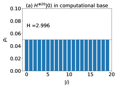
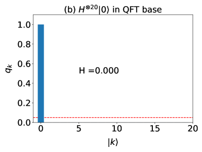
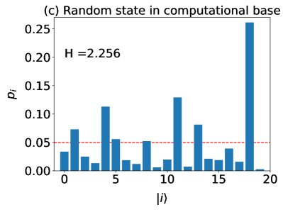
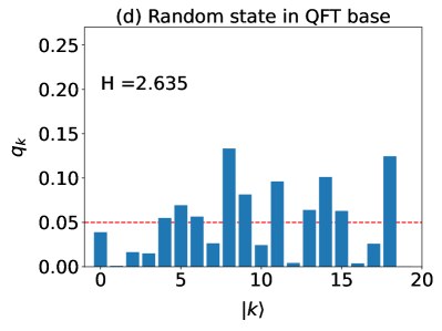
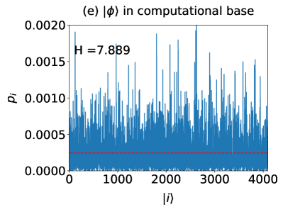
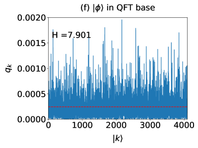
Figure 1: The distributions of $p_{i}$ for (a) a uniform superposition of all basis states $N=20$, (c) a random quantum state generated by a random unitary matrix ${\rm U}(N)$ with $N=20$, and (e) a random quantum state of $n=14$ qubits generated by a random quantum circuit implemented on the Sycamore processor [11, 23]. Plots (b), (d), and (f) are the distributions of $p_{k}$ after the quantum Fourier transform of (a), (b), and (c), respectively. The red lines indicate $p=1/N$ and the Shannon entropy $H$ for each state is labeled by $H$.

Note that the Shannon entropy $H(\left|{\psi}\right\rangle)$ is defined with respect to a specific basis set $\{\left|{i}\right\rangle\}$. If the same quantum state is expanded in terms of another basis set $\{\left|{k}\right\rangle\}$, $\left|{\psi}\right\rangle=\sum_{k=0}^{N-1}b_{k}\left|{k}\right\rangle$, its Shannon entropy $H(\left|{\psi}\right\rangle)$ will change. For two orthonormal basis sets, $\{\left|{i}\right\rangle\}$ and $\{\left|{k}\right\rangle\}$, the entropic uncertainty relation [24, 25, 26, 27] is written as

$$H(P)+H(Q)\geq-2\ln c$$ (5)

where $c=\max|\langle i|k\rangle|$, $P=(p_{0},\dots,p_{N-1})$ with $p_{i}=|a_{i}|^{2}$, and $Q=(q_{0},\dots,q_{N-1})$ with $q_{k}=|b_{k}|^{2}$. We consider the computational basis and the quantum Fourier transformed basis, which are mutually unbiased. The quantum Fourier transform (QFT) is the discrete Fourier transform of the amplitude vector $(x_{0},x_{1},\dots,x_{N-1})$ to another amplitude vector $(y_{0},y_{1},\dots,y_{N-1})$, defined by

$$y_{k}=\frac{1}{\sqrt{N}}\sum_{j=0}^{N-1}e^{i2\pi\frac{jk}{N}}\,x_{j}\,.$$ (6)

The QFT acting on $\left|{\psi_{P}}\right\rangle$ is written as

$$\left|{\psi_{P}}\right\rangle=\sum_{i=0}^{N-1}x_{i}\left|{i}\right\rangle\quad\longrightarrow\quad\left|{\psi_{Q}}\right\rangle=\sum_{k=0}^{N-1}y_{k}\left|{k}\right\rangle\,.$$ (7)

Fig. 1 illustrates the distributions of probabilities $p_{i}$ for two kinds of quantum states in the computational basis and probabilities $q_{k}$ in the QFT basis. First, consider a uniform superposition of all possible basis states in the computational basis that is given by $\left|{\psi}\right\rangle=\frac{1}{\sqrt{N}}(\left|{0}\right\rangle+\left|{1}\right\rangle+\cdots+\left|{N-1}\right\rangle)$. As shown in Fig. 1 (a), its $p_{i}$ is distributed uniformly, $p_{i}={1}/{N}$ with $i=0,1,\dots,N-1$ and its Shannon entropy has the maximum value, $H(P)=\ln(N)$. The equally-likely distribution among $N$ possible states implies the largest randomness, and the greatest entropy [28]. However, $\left|{\psi}\right\rangle$ in the QFT basis set is localized at one site, so its entropy $H(Q)$ is zero, as depicted in Fig. 1 (d). The entropic uncertainty is given by $H(P)+H(Q)=\ln(N)$. Next, consider a random quantum state $\left|{\phi}\right\rangle=U_{\rm Haar}\left|{0}\right\rangle$. Fig. 1 (b) plots the distribution of $p_{i}$ of a random quantum state where $U_{\rm Haar}$ is generated by the QR decomposition of an $N\times N$ complex Gaussian random matrix. The entropy of a random quantum state is approximately given by $H(P)=\ln N-1+\gamma\approx 2.302$ for $N=10$. Fig. 1 (e) plots the distribution of $q_{k}$ in the QFT basis. Interestingly, the entropy $H(P)$ of a random quantum state in the computational basis is almost equal to its entropy $H(Q)$ in its QFT basis. We observe that the average entropy for all random quantum states in the computational basis, generated by a random circuit $U$, is equal to that in the QFT basis. A random quantum state may have the balanced entropic uncertainty, $H(P)=H(Q)=\ln N-1+\gamma$. It is analogous to a coherent state in the sense that the latter has balanced or symmetric minimum uncertainty: $\Delta x=\Delta p$. It may be interesting to understand why a random quantum state is invariant under the QFT. Fig. 1 (c) depicts the distribution of $p_{i}$ for a random quantum state generated by a random quantum circuit implemented on the Sycamore processor for $n=12$ and the cycles $m=14$ [23]. Fig. 1 (f) plots the distribution of $q_{k}$ in the QFT basis. One can see that the Shannon entropy of a random quantum state in the computational basis is almost same as that of its QFT state. Note that the random circuit here is implemented on a classical computer without any noise. The Shannon entropy in Fig. 1 e is close to the theoretical value, $H=\ln N-1+\gamma\approx 7.8949$. The Shannon entropy calculated from the Sycamore data for $n=12$ and $m=14$ is $H\approx 8.217$ and close to $\ln(4096)\approx 8.31$ [29].

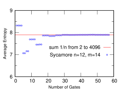
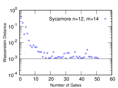
Figure 2: For a random quantum circuit for $n=14$ qubits and up to $m=14$ cycles [11], (a) Shannon entropy of the average of quantum states and (b) Wasserstein distance between the eigenvalues of random circuits and the Haar random unitary operator are plotted as a function of the number of gates applied, i.e., the depth of a quantum circuit.

Since a random quantum state is characterized by its Shannon entropy, $H(P)\approx\ln N-(1-\gamma)$, the Shannon entropy $H(\left|{\psi^{(k)}}\right\rangle)$ of a quantum state $\left|{\psi^{(k)}}\right\rangle=U_{k}\dots U_{1}\left|{0}\right\rangle$ at the $k$-th step of random walks could be used as a convergence measure to see whether the cutoff phenomenon happens. The sub-linear convergence proportional to $\sqrt{n}$ was claimed by calculating the average entropy of quantum states [17]. As shown in Fig. 2 (a), the Shannon entropy of a quantum state converges to $\ln N-(1-\gamma)$ as the number of gates increases and remains there. An interesting question is what happens to a quantum state after the Shannon entropy converges.

The eigenvalue distribution for random unitary operators drawn from the Haar measure is well known [21], so the distance between the eigenvalue distributions could be used to measure the convergence of a random walk. We consider the Wasserstein distance defined by

$$W_{p}(P,Q)=\left(\inf_{J\in J(P,Q)}\int||x-y||^{p}\,dJ(x,y)\right)^{1/p}\,,$$ (8)

where ${\cal J}(P,Q)$ denotes all joint distributions $J(P,Q)$. If $P$ and $Q$ are the empirical distributions of a data set $\{x_{1},\dots,x_{n}\}$ and $\{y_{1},\dots,y_{n}\}$ respectively, then the Wasserstein distance is given by the distance between order statistics

$$W_{p}(P,Q)=\left(\sum_{i=1}^{n}||x_{(i)}-y_{(i)}||^{p}\right)^{1/p}\,,$$ (9)

where $x_{(i)}$ is the $i$-th order statistic of a samples, i.e., its $i$-th smallest value. Fig. 2 (b) plots the Wasserstein distance of order 1 between the eigenvalue distribution of the circular unitary ensemble and that of a random quantum circuit as a function of the number of quantum gates applied. The calculation of the Wasserstein distance supports the cutoff phenomenon for random quantum circuits as the Shannon entropy does.

3 Dyson-Brownian Motions on a Unitary Group

In Sec. 2, the random walk on the unitary group is implemented by applying the sequence of random quantum circuits, $\{U_{1},U_{2},\dots\}$. A random quantum state after the $k$-th step is $\left|{\psi}\right\rangle=U_{k}\dots U_{1}\left|{0}\right\rangle$. This may be considered as a discrete process. In this section, we consider a continuous random walk given by a time-dependent random Hamiltonian to see how quickly a quantum state converges to a random quantum state. The time evolution operator at $t+\delta t$ is given by

$$U(t+\delta t) =e^{i\frac{\delta t}{\hbar}H(t)}\,U(t)$$ (10)

$$\approx\Bigl{[}1+i\frac{\delta t}{\hbar}H(t)-\frac{1}{2}\left(\frac{\delta t}{\hbar}\right)^{2}H^{2}(t)\Bigr{]}U(t)\,,$$ (11)

where $U(0)=I$. The time dependent random Hamiltonian $H(t)$ at time $t$ is obtained as follows. We draw a complex random matrix $A$ whose real and imaginary parts of a matrix element $A_{ij}$ are sampled independently from the normal distribution ${\cal N}(0,\sigma^{2}/2N)$ with the variance $\sigma^{2}/2N$. The Hermitian property of the Hamiltonian $H$ is fulfilled by summing $A$ and its conjugate transpose $A^{\dagger}$, $H=\frac{1}{2}(A+A^{\dagger})$. $H$ is the elements of the Gaussian orthogonal ensemble.

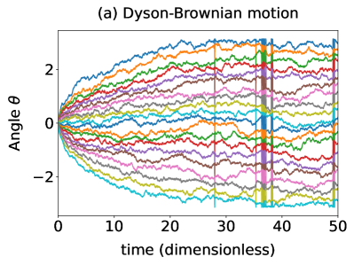
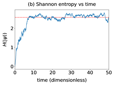
Figure 3: For the Dyson-Brownian random walk, (a) trajectories of eigenvalues of a random unitary operator and (b) the Shannon entropy $H(\left|{\psi}\right\rangle)$ of a quantum state are plotted. Here, we take $20\times 20$ random Hamiltonian matrices, i.e., $N=20$ and the time step $\delta t=0.01$. In (b) the red dotted horizontal line represents the Shannon entropy of a random quantum state, $\ln N-1+\gamma\approx 2.5572$ for $N=20$.

The trajectories of eigenvalues of a random unitary operator $U$ are known as the Dyson-Brownian motions and do not overlap with others. Eigenvalues repel each other. We simulate the time evolution with a time-dependent random Hamiltonian for $N=20$ and $\sigma=1$ so $\sigma^{2}/2N=1/2N$. For simplicity, we take $\hbar=1$. We set the time step $\delta t=0.01$. The eigenvalues of $U(t)$ from Eq. (11) are obtained by diagonalizing it and their trajectories as a function of time are plotted in Fig. 3 (a). The time-evolution of the Shannon entropy of a quantum state $\left|{\psi(t)}\right\rangle=U(t)\left|{0}\right\rangle$ is shown in Fig. 3 (b). We observe the non-asymptotic convergence to $\ln N-1+\gamma\approx 2.5572$ for $N=20$. It is interesting to see the eigenvalues and the Shannon entropy fluctuate after arriving at the steady state. Particularly, the fluctuation in the Shannon entropy in Fig. 3 (b) is in contrast to no fluctuation in the Shannon entropy for a finite random walk of a random quantum circuit, shown in Fig. 1 (a).

4 Summary

In this paper, we examined some properties of random quantum states generated by discrete and continuous random walks on a unitary group. It is found that the Shannon entropy of a random quantum state generated by random quantum circuits is invariant under the QFT in the sense that the Shannon entropy does not change before and after applying the QFT. The entropic uncertainty relation of a random quantum state for the computational bases and the QFT bases is balanced, i.e., $H(P)=H(Q)$. This may remind us of the coherent state with the balanced minimum uncertainty relation, $\delta x=\delta p$. We showed that the cutoff phenomenon for a random quantum circuit occurs by calculating the Shannon entropy and the Wasserstein distance for the eigenvalue distributions. It is a open question whether the cutoff of random walks on a unitary group scales with the number of qubits $n$ as sub-linear ${\cal O}(\sqrt{n})$ or ${\cal O}({n}2^{n})$ while the numerical calculations here seem to support the sub-linear scaling of the cutoff.

In addition to the demonstration of quantum advantage, random quantum circuits may be applicable to solving interesting problems, for example, in randomized linear algebra. The set of random quantum states $\left|{\psi_{i}}\right\rangle=U_{\rm Haar}\left|{i}\right\rangle$ with $i=0,1,\dots,2^{n}-1$ form the orthonormal basis set. The trace of a matrix $A$ could be calculated using ${\rm Tr}(A)\approx\frac{1}{M}\sum_{i=1}^{M}\left\langle{\psi_{i}}\right|A\left|{\psi_{i}}\right\rangle$ where $\left|{\psi_{i}}\right\rangle$ is a random quantum state [30].

References

References

- [1] Aldous D and Diaconis P 1986 The American Mathematical Monthly 93 333–348 ISSN 00029890, 19300972 URL http://www.jstor.org/stable/2323590
- [2] Bayer D and Diaconis P 1992 The Annals of Applied Probability 2 294 – 313 URL https://doi.org/10.1214/aoap/1177005705
- [3] Diaconis P 1996 Proceedings of the National Academy of Sciences 93 1659–1664 URL https://www.pnas.org/doi/pdf/10.1073/pnas.93.4.1659
- [4] Ehrenfest P and Ehrenfest-Afanassjewa T 1907 Über zwei bekannte Einwände gegen das Boltzmannsche H-Theorem (Hirzel)
- [5] Diaconis P, Graham R L and Morrison J A 1990 Random Structures & Algorithms 1 51–72 (Preprint https://onlinelibrary.wiley.com/doi/pdf/10.1002/rsa.3240010105) URL https://onlinelibrary.wiley.com/doi/abs/10.1002/rsa.3240010105
- [6] Lubetzky E and Sly A 2013 Inventiones mathematicae 191 719–755 ISSN 1432-1297 URL https://doi.org/10.1007/s00222-012-0404-5
- [7] Kastoryano M J, Reeb D and Wolf M M 2012 Journal of Physics A: Mathematical and Theoretical 45 075307 URL https://dx.doi.org/10.1088/1751-8113/45/7/075307
- [8] Rosenthal J S 1994 The Annals of Probability 22 398 – 423 URL https://doi.org/10.1214/aop/1176988864
- [9] Porod U 1996 The Annals of Probability 24 74–96 ISSN 00911798 URL http://www.jstor.org/stable/2244833
- [10] Porod U 1996 Probability Theory and Related Fields 104 181–209 ISSN 1432-2064 URL https://doi.org/10.1007/BF01247837
- [11] Arute F, Arya K, Babbush R, Bacon D, Bardin J C, Barends R, Biswas R, Boixo S, Brandao F G S L, Buell D A, Burkett B, Chen Y, Chen Z, Chiaro B, Collins R, Courtney W, Dunsworth A, Farhi E, Foxen B, Fowler A, Gidney C, Giustina M, Graff R, Guerin K, Habegger S, Harrigan M P, Hartmann M J, Ho A, Hoffmann M, Huang T, Humble T S, Isakov S V, Jeffrey E, Jiang Z, Kafri D, Kechedzhi K, Kelly J, Klimov P V, Knysh S, Korotkov A, Kostritsa F, Landhuis D, Lindmark M, Lucero E, Lyakh D, Mandrà S, McClean J R, McEwen M, Megrant A, Mi X, Michielsen K, Mohseni M, Mutus J, Naaman O, Neeley M, Neill C, Niu M Y, Ostby E, Petukhov A, Platt J C, Quintana C, Rieffel E G, Roushan P, Rubin N C, Sank D, Satzinger K J, Smelyanskiy V, Sung K J, Trevithick M D, Vainsencher A, Villalonga B, White T, Yao Z J, Yeh P, Zalcman A, Neven H and Martinis J M 2019 Nature 574 505–510 ISSN 0028-0836, 1476-4687 URL http://www.nature.com/articles/s41586-019-1666-5
- [12] Wu Y, Bao W S, Cao S, Chen F, Chen M C, Chen X, Chung T H, Deng H, Du Y, Fan D, Gong M, Guo C, Guo C, Guo S, Han L, Hong L, Huang H L, Huo Y H, Li L, Li N, Li S, Li Y, Liang F, Lin C, Lin J, Qian H, Qiao D, Rong H, Su H, Sun L, Wang L, Wang S, Wu D, Xu Y, Yan K, Yang W, Yang Y, Ye Y, Yin J, Ying C, Yu J, Zha C, Zhang C, Zhang H, Zhang K, Zhang Y, Zhao H, Zhao Y, Zhou L, Zhu Q, Lu C Y, Peng C Z, Zhu X and Pan J W 2021 Phys. Rev. Lett. 127(18) 180501 URL https://link.aps.org/doi/10.1103/PhysRevLett.127.180501
- [13] Zhu Q, Cao S, Chen F, Chen M C, Chen X, Chung T H, Deng H, Du Y, Fan D, Gong M, Guo C, Guo C, Guo S, Han L, Hong L, Huang H L, Huo Y H, Li L, Li N, Li S, Li Y, Liang F, Lin C, Lin J, Qian H, Qiao D, Rong H, Su H, Sun L, Wang L, Wang S, Wu D, Wu Y, Xu Y, Yan K, Yang W, Yang Y, Ye Y, Yin J, Ying C, Yu J, Zha C, Zhang C, Zhang H, Zhang K, Zhang Y, Zhao H, Zhao Y, Zhou L, Lu C Y, Peng C Z, Zhu X and Pan J W 2022 Science Bulletin 67 240–245 ISSN 2095-9273 URL https://www.sciencedirect.com/science/article/pii/S2095927321006733
- [14] Oh S and Kais S 2022 The Journal of Physical Chemistry Letters 13 7469–7475 pMID: 35939529 URL https://doi.org/10.1021/acs.jpclett.2c02045
- [15] Oh S and Kais S 2022 Phys. Rev. A 106(3) 032433 URL https://link.aps.org/doi/10.1103/PhysRevA.106.032433
- [16] Oh S and Kais S 2023 Phys. Rev. A 107(2) 022610 URL https://link.aps.org/doi/10.1103/PhysRevA.107.022610
- [17] Boixo S, Isakov S V, Smelyanskiy V N, Babbush R, Ding N, Jiang Z, Bremner M J, Martinis J M and Neven H 2018 Nature Physics 14 595–600 ISSN 1745-2481 URL https://doi.org/10.1038/s41567-018-0124-x
- [18] Emerson J, Weinstein Y S, Saraceno M, Lloyd S and Cory D G 2003 Science 302 2098–2100 ISSN 0036-8075 URL https://science.sciencemag.org/content/302/5653/2098
- [19] Haake F, Gnutzmann S and Kuś M 2010 Quantum Signatures of Chaos (Springer-Verlag Berlin Heidelberg) ISBN 978-3-642-05428-0
- [20] Mezzadri F 2007 Notices of the American Mathematical Society 54 592 – 604 ISSN 0002-9920
- [21] Meckes E S 2019 The Random Matrix Theory of the Classical Compact Groups Cambridge Tracts in Mathematics (Cambridge University Press)
- [22] Ozols M 2009 unpublished essay on http://home. lu. lv/sd20008
- [23] Martinis et al J M 2022 Quantum supremacy using a programmable superconducting processor, Dryad, Dataset https://doi.org/10.5061/dryad.k6t1rj8
- [24] Deutsch D 1983 Phys. Rev. Lett. 50(9) 631–633 URL https://link.aps.org/doi/10.1103/PhysRevLett.50.631
- [25] Kraus K 1987 Phys. Rev. D 35(10) 3070–3075 URL https://link.aps.org/doi/10.1103/PhysRevD.35.3070
- [26] Maassen H and Uffink J B M 1988 Phys. Rev. Lett. 60(12) 1103–1106 URL https://link.aps.org/doi/10.1103/PhysRevLett.60.1103
- [27] Coles P J, Berta M, Tomamichel M and Wehner S 2017 Rev. Mod. Phys. 89(1) 015002 URL https://link.aps.org/doi/10.1103/RevModPhys.89.015002
- [28] Ambegaokar V and Clerk A A 1999 American Journal of Physics 67 1068–1073 ISSN 0002-9505 (Preprint https://pubs.aip.org/aapt/ajp/article-pdf/67/12/1068/10115996/1068_1_online.pdf) URL https://doi.org/10.1119/1.19084
- [29] Oh S and Kais S (unpublished)
- [30] Oh S and Kais S (in preparation) Estimating trace of a matrix with random quantum states