Accelerated DC Algorithms for the Asymmetric Eigenvalue Complementarity Problem

Abstract.

We are interested in solving the Asymmetric Eigenvalue Complementarity Problem (AEiCP) by accelerated Difference-of-Convex (DC) algorithms. Two novel hybrid accelerated DCA: the Hybrid DCA with Line search and Inertial force (HDCA-LI) and the Hybrid DCA with Nesterov’s extrapolation and Inertial force (HDCA-NI), are established. We proposed three DC programming formulations of AEiCP based on Difference-of-Convex-Sums-of-Squares (DC-SOS) decomposition techniques, and applied the classical DCA and 6 accelerated variants (BDCA with exact and inexact line search, ADCA, InDCA, HDCA-LI and HDCA-NI) to the three DC formulations. Numerical simulations of 7 DCA-type methods against state-of-the-art optimization solvers IPOPT, KNITRO and FILTERSD, are reported.

1. Introduction

Asymmetric Eigenvalue Complementarity Problem (AEiCP) consists of finding complementary eigenvectors $x\in\operatorname{\mathbb{R}}^{n}\setminus\{0\}$ and complementary eigenvalues $\lambda\in\operatorname{\mathbb{R}}$ such that

(AEiCP) $$\begin{cases}w=\lambda Bx-Ax,\\ x^{\top}w=0,\\ 0\neq x\geq 0,w\geq 0.\end{cases}$$

where $x^{\top}$ is the transpose of $x$, $A\in\operatorname{\mathbb{R}}^{n\times n}$ is an asymmetric real matrix, and $B$ is a positive definite ($\operatorname{PD}$) matrix (unnecessarily to be symmetric). If $A$ and $B$ are both symmetric, then the problem is called symmetric EiCP (SEiCP). Throughout the paper, we will denote the solution set of problem (AEiCP) (resp. SEiCP) by $\text{AEiCP}(A,B)$ (resp. $\text{SEiCP}(A,B)$). The Eigenvalue Complementarity Problem appeared in the study of static equilibrium states of mechanical systems with unilateral friction [38], and found interest in the Spectral Theory of Graphs [12, 41].

In [19, Theorem 2.1], it is known that (AEiCP) can be expressed as a finite variational inequality on the unit simplex $\Omega:=\{x\in\operatorname{\mathbb{R}}^{n}:e^{\top}x=1,x\geq 0\}$, which involves finding $\bar{x}\in\Omega$ satisfying:

$$\left\langle\left(\frac{x^{\top}Ax}{x^{\top}Bx}B-A\right)x,x-\bar{x}\right\rangle\geq 0,\quad\forall x\in\Omega.$$

If $B$ is a strictly copositive ($\operatorname{SC}$) matrix (i.e., $x^{\top}Bx>0$ for all $x\geq 0$ and $x\neq 0$), then the variational inequality is guaranteed to have a solution [10]. Hence, (AEiCP) has a solution since $B\in\operatorname{PD}$ (a special case of $B\in\operatorname{SC}$). Moreover, (AEiCP) has at most $n2^{n-1}$ distinct $\lambda$-solutions [39, Proposition 3], and it has a positive complementary eigenvalue if $A$ is a copositive matrix (i.e., $x^{\top}Ax\geq 0,\forall x\geq 0$) and $-A$ is a $R_{0}$ matrix (i.e., $M\in R_{0}$ if and only if $[x\geq 0,Mx\geq 0,x^{\top}Mx=0]\Rightarrow x=0$) [19, Theorem 2.2]. In particular, when both $A,B\in\operatorname{PD}$, then all complementary eigenvalues of (AEiCP) are positive. If $A$ is not $\operatorname{PD}$, then we can find some $\mu>0$ such that $A+\mu B\in\operatorname{PD}$ and, as shown in [25, Theorem 2.1], we have:

$$(x,\lambda)\in\text{EiCP}(A,B)\Leftrightarrow(x,\lambda+\mu)\in\text{EiCP}(A+\mu B,B).$$

Without loss of generality, throughout the paper, we assume that:

Hypothesis 1.1.

Both $A$ and $B$ are PD matrices for (AEiCP).

In fact, solving the SEiCP is much easier than the AEiCP. For the SEiCP, there are three well-known equivalent formulations (see e.g., [25]), namely the Rayleigh quotient formulation

(RP) $$\max\left\{\frac{x^{\top}Ax}{x^{\top}Bx}:x\in\Omega\right\},$$

the logarithmic formulation

(LnP) $$\max\left\{\ln(x^{\top}Ax)-\ln(x^{\top}Bx):x\in\Omega\right\},$$

and the quadratic formulation

(QP) $$\max\{x^{\top}Ax:x^{\top}Bx\leq 1,x\geq 0\}.$$

These formulations are equivalent to SEiCP in the sense that if $\bar{x}$ is a stationary point of (QP), (RP) or (LnP), then

$$(\bar{x},(\bar{x}^{\top}A\bar{x})/(\bar{x}^{\top}B\bar{x}))\in\text{SEiCP}(A,B).$$

However, they are no longer equivalent to (AEiCP). A simple convincing counterexample is given below: Let $n=2$, $B=I_{2}$ and

$$A=\begin{bmatrix}-1&1\\ -2&2\end{bmatrix}.$$

Then, the vector $\bar{x}=[0,1]^{\top}$ is a stationary point of (QP), (RP) and (LnP), but

$$(\bar{x},(\bar{x}^{\top}A\bar{x})/(\bar{x}^{\top}B\bar{x}))=([0,1]^{\top},2)\notin\text{AEiCP}(A,B)$$

because

$$\bar{w}=(\bar{x}^{\top}A\bar{x})/(\bar{x}^{\top}B\bar{x})B\bar{x}-A\bar{x}=\begin{bmatrix}-1\\ 0\end{bmatrix}\leq 0.$$

In fact $([0,1]^{\top},2)\in\text{SEiCP}(A+A^{\top},B+B^{\top})$, but $\text{SEiCP}(A+A^{\top},B+B^{\top})$ and $\text{AEiCP}(A,B)$ are not equivalent for (AEiCP). Hence, we can not get a solution of (AEiCP) by searching a stationary point of (QP), (RP) or (LnP).

Concerning solution algorithms for (AEiCP), a number of algorithms have been designed such as Enumerative method [19, 11], Semismooth Newton method [1], Descent algorithm for minimizing the regularized gap function [7], Difference-of-Convex (DC) algorithm [28, 26, 27, 25], Splitting algorithm [15], Active-set method [6], Projected-Gradient algorithm [17], and Alternating Direction Method of Multipliers (ADMM) [16]. Most of these methods can be applied to both AEiCP and SEiCP. However, despite the theoretical ability of the Enumerative method to always find a solution to (AEiCP), its practical application often proves computationally demanding or even intractable for larger instances within reasonable CPU time. The other algorithms face the same drawback, that is they attempt to solve nonconvex optimization formulations using local optimization approaches, which may fail for many instances in (AEiCP), particularly when solution accuracy is on demand and at least one of the matrices $A$ and $B$ is ill-conditioned.

In this paper, we will focus on solving three nonlinear programming (NLP) formulations of (AEiCP) via several accelerated DCA. First, we present in Section 2 the classical DCA and three accelerated variants of DCA (BDCA [3, 29], ADCA [36] and InDCA [9, 43]) for solving the convex constrained DC programming problem with polynomial objective function over a closed convex set. Then, the spotlight is on establishing two novel hybrid accelerated DCA, namely the Hybrid DCA with Line search and Inertial force (HDCA-LI) and the Hybrid DCA with Nesterov’s extrapolation and Inertial force (HDCA-NI). A rigorous convergence analysis for both HDCAs is furnished. In Section 3, we delve into establishing three DC programming formulations for (AEiCP) by leveraging the DC-SOS decomposition techniques [23], acclaimed for generating superior quality DC decompositions of polynomials. Following this, we discuss in Sections 4 and 5 the application of the aforementioned accelerated variants of DCA in solving the three DC formulations of (AEiCP). Finally, in Section 6, we report numerical simulations comparing the proposed $7$ DCA-type algorithms with cutting-edge NLP solvers, namely IPOPT, KNITRO, and FILTERSD, and demonstrate their numerical performance on some large-scale and ill-conditioned instances.

2. Accelerated DC Algorithms

Consider the convex constrained DC (Difference-of-Convex) program defined by

(P) $$\min_{x\in\operatorname{\mathcal{C}}}\{f(x):=g(x)-h(x)\},$$

where $\operatorname{\mathcal{C}}$ is a nonempty closed and convex subset of a finite dimensional Euclidean space endowed with an inner product $\langle\cdot,\cdot\rangle$ and an induced norm $\|\cdot\|$. Both $g$ and $h$ are convex polynomials such that $g$ (resp. $h$) is $\rho_{g}$-convex with $\rho_{g}\geq 0$ (resp. $\rho_{h}$-convex with $\rho_{g}\geq 0$) over $\operatorname{\mathcal{C}}$, i.e., $g(\cdot)-\frac{\rho_{g}}{2}\|\cdot\|^{2}$ (resp. $h(\cdot)-\frac{\rho_{h}}{2}\|\cdot\|^{2}$) is convex over $\operatorname{\mathcal{C}}$. If $\rho_{g}>0$ (resp. $\rho_{h}>0$), then $g$ (resp. $h$) is called $\rho_{g}$ (resp. $\rho_{h}$) strongly convex over $\operatorname{\mathcal{C}}$.

In this section, we briefly introduce the standard DCA and three existing accelerated variants of DCA, namely BDCA, ADCA, and InDCA, for solving (P). Following that, we propose two novel hybrid accelerated DCAs: the Hybrid DCA with Line search and Inertial force (HDCA-LI) and the Hybrid DCA with Nesterov’s extrapolation and Inertial force (HDCA-NI). We also provide their convergence analysis. Some characteristics of these DCA-type algorithms are summarized in Table 1, where the columns Linesearch, Inertial, and Nesterov indicate whether the algorithm requires a line search, heavy-ball inertial force, and Nesterov’s extrapolation, respectively. The monotone column represents the monotonicity of the generated sequence $\{f(x^{k})\}$.

Table 1. Some characteristics of the DCA-type algorithms.

Algorithm	Linesearch	Inertial	Nesterov	Monotone
DCA [32]	✗	✗	✗	✓
BDCA [29]	✓	✗	✗	✓
ADCA [36]	✗	✗	✓	✗
InDCA [9, 43]	✗	✓	✗	✗
HDCA-LI	✓	✓	✗	✗
HDCA-NI	✗	✓	✓	✗

2.1. DCA

One of the most renowned algorithm for solving (P) is called DCA, which is first introduced by Pham Dinh Tao in 1985 as an extension of the subgradient method [35], and extensively developed by Le Thi Hoai An and Pham Dinh Tao since 1994 (see [32, 33, 34, 22] and the references therein).

DCA applied to (P) consists of constructing a sequence $\{x^{k}\}$ by solving the convex subproblems:

(DCA) $$\boxed{x^{k+1}\in\operatorname{argmin}\{g(x)-\langle x,\nabla h(x^{k})\rangle:x\in\operatorname{\mathcal{C}}\},}$$

that is, minimizing the convex majorant (cf. surrogate) of the DC function $f$ at iterate $x^{k}$ in form of $g(x)-[h(x^{k})+\langle\nabla h(x^{k}),x-x^{k}\rangle]$ by linearizing $h$ at $x^{k}$.

DCA is a descent method enjoys the next convergence properties:

Theorem 2.1 (Convergence theorem of DCA for (P), see e.g., [32, 24, 29]).

Let $\{x^{k}\}$ be a well-defined sequence generated by DCA for problem (P) from an initial point $x^{0}\in\operatorname{\mathbb{R}}^{n}$. If $\inf\{f(x):x\in\operatorname{\mathcal{C}}\}>-\infty$ and the sequence $\{x^{k}\}$ is bounded, then

• (monotonicity and convergence of $\{f(x^{k})\}$) the sequence $\{f(x^{k})\}$ is non-increasing and convergent.

• (sufficiently descent property)

  $$f(x^{k})-f(x^{k+1})\geq\frac{\rho_{g}+\rho_{h}}{2}\|x^{k}-x^{k+1}\|^{2},\quad\forall k\geq 1.$$

• (square summable property) if $\rho_{g}+\rho_{h}>0$, then

  $$\sum_{k\geq 0}\|x^{k+1}-x^{k}\|^{2}<\infty.$$

• (subsequential convergence of $\{x^{k}\}$) any cluster point $x^{*}$ of the sequence $\{x^{k}\}$ is a critical point of (P), i.e., $\nabla h(x^{*})\in\partial(g+\chi_{\operatorname{\mathcal{C}}})(x^{*})$.

• (convergence of $\{x^{k}\}$) if $f$ is a KL function, $\rho_{g}+\rho_{h}>0$, $h$ has locally Lipschitz continuous gradient over $\operatorname{\mathcal{C}}$, and $\operatorname{\mathcal{C}}$ is a semi-algebraic set, then the sequence $\{x^{k}\}$ is convergent.

Remark 2.2.

• DCA is a monotone algorithm in the sequence $\{f(x^{k})\}$.

• The symbol $\partial$ denotes the subdifferential of the convex function [40] and $\chi_{\operatorname{\mathcal{C}}}$ is the indicator function defined as $\chi_{\operatorname{\mathcal{C}}}(x)=0$ if $x\in\operatorname{\mathcal{C}}$ and $\chi_{\operatorname{\mathcal{C}}}(x)=\infty$ otherwise.

• $\inf\{f(x):x\in\operatorname{\mathcal{C}}\}>-\infty$ does not necessarily imply that the sequence $\{x^{k}\}$ is bounded. For instance, consider $g(x)=e^{x}$, $h(x)=0$ and $\operatorname{\mathcal{C}}=\operatorname{\mathbb{R}}$. Clearly, $\inf\{f(x):x\in\operatorname{\mathcal{C}}\}=0>-\infty$. Then, DCA starting from any initial point $x^{0}\in\operatorname{\mathbb{R}}$ will generate a sequence $\{x^{k}\}$ that tends to $\infty.$ Conversely, it is obvious that the existence of a bounded sequence $\{x^{k}\}$ does not imply that $\inf_{x\in\operatorname{\mathcal{C}}}f(x)>-\infty$.

• Without the assumption $\inf_{x\in\operatorname{\mathcal{C}}}f(x)>-\infty$, then the convergence of $\{f(x^{k})\}$ may not be true; without the boundedness assumptions of $\{x^{k}\}$, then a cluster point of $\{x^{k}\}$ may not exist; without the assumption $\rho_{g}+\rho_{h}>0$, then $\|x^{k+1}-x^{k}\|\to 0$ may not be true, and thus a limit point of $\{x^{k}\}$ may not be a critical point of (P) (see the corresponding counterexamples in [24]).

• The strong convexity assumption in $g$ or $h$ is not restrictive and can be easily guaranteed in practice, since we can introduce the regularity term $\frac{\rho}{2}\|x\|^{2}$ (for any $\rho>0$) into $g$ and $h$ for getting a satisfactory DC decomposition as

  $$\underbrace{(g(x)+\frac{\rho}{2}\|x\|^{2})}_{=\tilde{g}(x)}-\underbrace{(h(x)+\frac{\rho}{2}\|x\|^{2})}_{=\tilde{h}(x)},$$

  where both $\tilde{g}$ and $\tilde{h}$ are $\rho$-strongly convex.

• The KL (Kurdyka-Łajasiewicz) assumption plays an important role to guarantee the convergence of the whole sequence $\{x^{k}\}$, which is an immediate consequence of [24, Theorem 5] (see also [21]). The KL function is a function satisfying the well-known KL property (see e.g., [24, Definition 3]), which is ubiquitous in optimization and its applications, e.g., the semialgebraic, subanalytic, log and exp are KL functions (see [20, 5, 4] and the references therein). In particular, for a closed convex semi-algebraic set $\operatorname{\mathcal{C}}$ (i.e., $\operatorname{\mathcal{C}}$ is a set of polynomial equations and inequalities) and the objective function $f$ has a polynomial DC decomposition $g-h$ where $g$ and $h$ are $\rho_{g}$- and $\rho_{h}$-convex polynomials over $\operatorname{\mathcal{C}}$ with $\rho_{g}+\rho_{h}>0$, then the convergence of $\{x^{k}\}$ is guaranteed.

2.2. BDCA

BDCA is an accelerated DCA by introducing the (exact or inexact) line search into DCA for acceleration. It was first proposed by Artacho et al. in 2018 [3] for unconstrained smooth DC program with the Armijo line search, then extended by Niu et al. in 2019 [29] for general convex constrained smooth and nonsmooth DC programs with both exact and inexact line searches.

The general idea of BDCA in [29] is to introduce a line search along the DC descent direction (a feasible and descent direction generated by two consecutive iterates of DCA) $d^{k}:=z^{k}-x^{k}$ to find a better candidate $x^{k+1}$, where

$$z^{k}\in\operatorname{argmin}\{g(x)-\langle y^{k},x\rangle\},\quad y^{k}\in\partial h(x^{k}).$$

The line search can be performed either exactly ($=$) or inexactly ($\approx$) to find an optimal solution or an approximate solution of the line search problem

$$\alpha_{k}=\text{or}\approx\operatorname{argmin}\{f(z^{k}+\alpha d^{k}):z^{k}+\alpha d^{k}\in\operatorname{\mathcal{C}},\alpha\geq 0\}$$

with $f(z^{k}+\alpha d^{k})\leq f(z^{k})$. Then we update $x^{k+1}$ by

$$x^{k+1}=x^{k}+\alpha_{k}d^{k}.$$

BDCA for problem (P) is summarized in Algorithm 1.

Algorithm 1 BDCA for (P)

0:  $x^{0}\in\operatorname{\mathbb{R}}^{n}$, $\bar{\alpha}>0$;

1:  for $k=0,1,\ldots$ do

2:     $z^{k}\in\operatorname{argmin}\{g(x)-\langle x,\nabla h(x^{k})\rangle:x\in\operatorname{\mathcal{C}}\}$;

3:     initialize $x^{k+1}\leftarrow z^{k}$;

4:     $d^{k}\leftarrow z^{k}-x^{k}$;

5:     if $\operatorname{\mathcal{A}}(z^{k})\subset\operatorname{\mathcal{A}}(x^{k})$ and $\langle\nabla f(z^{k}),d^{k}\rangle<0$ then

6:        $x^{k+1}\leftarrow\text{LineSearch}(z^{k},d^{k},\bar{\alpha})$;

7:     end if

8:  end for

Some comments regarding Algorithm 1 include:

• DCA for (P) is just BDCA without the codes between line 4 to 7.

• For proceeding the line search, we have to check the conditions $\operatorname{\mathcal{A}}(z^{k})\subset\operatorname{\mathcal{A}}(x^{k})$ and $\langle\nabla f(z^{k}),d^{k}\rangle<0$ in line 5, where $\operatorname{\mathcal{A}}(x^{k})$ is the active set of $\operatorname{\mathcal{C}}$ at $x^{k}$. These are sufficient conditions for a DC descent direction, but not necessary when $\operatorname{\mathcal{C}}$ is not a polyhedral set. In fact, it was proven in [29] that $d^{k}$ is a ‘potentially’ descent direction of $f$ at $z^{k}$ such that

  • if $f^{\prime}(z^{k};d^{k})<0$, then $d^{k}$ is a descent direction of $f$ at $z^{k}$;

  • if $\operatorname{\mathcal{C}}$ is polyhedral, then $\operatorname{\mathcal{A}}(z^{k})\subset\operatorname{\mathcal{A}}(x^{k})$ is a necessary and sufficient condition for $d^{k}$ to be a feasible direction at $z^{k}$;

  • if $\operatorname{\mathcal{C}}$ is not polyhedral, then $\operatorname{\mathcal{A}}(z^{k})\subset\operatorname{\mathcal{A}}(x^{k})$ is just a necessary (but not always sufficient) condition for $d^{k}$ to be a feasible direction at $z^{k}$.

• The line search procedure LineSearch($z^{k}$,$d^{k}$,$\bar{\alpha}$) in line 6 can be either exact or inexact, depending on the problem size and structure. Generally speaking, finding an exact solution for $\alpha_{k}$ is computationally expensive or intractable when the problem size is too large or the objective function $f$ is too complicated. In this case, we suggest finding an approximate solution for $\alpha_{k}$ using an inexact line search procedure such as Armijo-type, Goldstein-type, or Wolfe-type [30, Chapter 3]. The third parameter $\bar{\alpha}$ denotes a given upper bound for the line search stepsize such that $\alpha_{k}\in[0,\bar{\alpha}]$ verifying $f(x^{k+1})\leq f(z^{k})$ with

  $$x^{k+1}=z^{k}+\alpha_{k}d^{k},\quad k=0,1,2,\ldots.$$

  Note that for exact line search with unbounded set $\operatorname{\mathcal{C}}$, if without $\bar{\alpha}$ (i.e., $\bar{\alpha}=\infty$), then the sequence $\{\alpha_{k}\}$ may be unbounded. Consequently, we impose $\bar{\alpha}$ to ensure the boundedness of the sequence $\{\alpha_{k}\}$, which is crucial for the well-definedness of the sequence $\{x^{k}\}$ and the convergence of the algorithm BDCA. See successful examples of BDCA with inexact Armijo-type line search in [29] and with exact line search in [44] for higher-order moment portfolio optimization problem, as well as BDCA with exact line search in [25] for symmetric eigenvalue complementarity problem.

BDCA enjoys the next convergence theorem:

Theorem 2.3 (Convergence theorem of BDCA Algorithm 1, see [24, 29]).

Let $\{x^{k}\}$ be a well-defined and bounded sequence generated by BDCA Algorithm 1 for problem (P) from an initial point $x^{0}\in\operatorname{\mathbb{R}}^{n}$. If $\rho_{g}+\rho_{h}>0$ and the solution set of (P) is non-empty, then

• (monotonicity and convergence of $\{f(x^{k})\}$) the sequence $\{f(x^{k})\}$ is non-increasing and convergent.

• (convergence of $\{\|x^{k}-z^{k}\|\}$ and $\{\|x^{k}-x^{k-1}\|\}$)

  $$\|x^{k}-z^{k}\|\xrightarrow{k\to\infty}0\quad\text{ and }\quad\|x^{k}-x^{k-1}\|\xrightarrow{k\to\infty}0.$$

• (subsequential convergence of $\{x^{k}\}$) any cluster point of the sequence $\{x^{k}\}$ is a critical point of (P).

• (convergence of $\{x^{k}\}$) furthermore, if $f$ is a KL function, $\operatorname{\mathcal{C}}$ is a semi-algebraic set, and $h$ has locally Lipschitz continuous gradient over $\operatorname{\mathcal{C}}$, then the sequence $\{x^{k}\}$ is convergent.

Remark 2.4.

BDCA, like the standard DCA, is a descent method. Theorem 2.3 is an immediate consequence of the general convergence theorem of BDCA for convex constrained nonsmooth DC programs established in [29]. Remark 2.2 for standard DCA is adopted here as well.

2.3. ADCA

ADCA is an accelerated DCA by introducing the Nesterov’s acceleration into DCA, which is introduced by Phan et al. in 2018 [36].

The basic idea of ADCA is to compute $\nabla h(v^{k})$ instead of $\nabla h(x^{k})$ at iteration $k$, where $v^{k}$ is a more promising point than $x^{k}$ in the sense that $v^{k}$ is better than one of the last $q$ iterates $\{x^{k-q},\ldots,x^{k}\}$ in terms of objective function, i.e.,

(2.1) $$f(v^{k})\leq\max_{t=\max\{0,k-q\},\ldots,k}f(x^{t}).$$

The candidate $v^{k}$ is computed by Nesterov’s extrapolation:

$$v^{k}=x^{k}+\frac{\theta_{k}-1}{\theta_{k+1}}\left(x^{k}-x^{k-1}\right),$$

where

$$\theta_{0}=1,\quad\theta_{k+1}=\frac{1+\sqrt{1+4\theta_{k}^{2}}}{2},\quad\forall k\geq 1.$$

If the condition (2.1) is not satisfied, then we set $v^{k}=x^{k}$ as in DCA.

ADCA applied to problem (P) is described below:

Algorithm 2 ADCA for (P)

0:  $x^{0}\in\operatorname{\mathbb{R}}^{n}$, $q\in\operatorname{\mathbb{N}}$;

1:  Initialization: $x^{-1}=x^{0}$, $\theta_{0}=1$;

2:  for $k=0,1,\ldots$ do

3:     $\theta_{k+1}\leftarrow\frac{1+\sqrt{1+4\theta_{k}^{2}}}{2}$;

4:     $v^{k}\leftarrow x^{k}+\frac{\theta_{k}-1}{\theta_{k+1}}\left(x^{k}-x^{k-1}\right);$

5:     if $f(v^{k})>\max\{f(x^{t}):t=\max\{0,k-q\},\ldots,k\}$ then

6:        $v^{k}\leftarrow x^{k};$

7:     end if

8:     $x^{k+1}\in\operatorname{argmin}\{g(x)-\langle x,\nabla h(v^{k})\rangle:x\in\operatorname{\mathcal{C}}\}$;

9:  end for

Remark 2.5.

ADCA is a non-monotone algorithm due to the introduction of Nesterov’s extrapolation. It acts as a descent method when $q=0$. In this case, we choose a better candidate in terms of the objective value between $v^{k}$ and $x^{k}$ to compute $x^{k+1}$. If $q>0$, then ADCA can increase the objective function and consequently escape from a potential bad local minimum. A higher value of $q$ increases the chance of escaping bad local minima.

ADCA enjoys the next convergence theorem:

Theorem 2.6 (Convergence theorem of ADCA Algorithm 2, see [36]).

Let $\{x^{k}\}$ be the sequence generated by ADCA Algorithm 2 for problem (P) from any initial point $x^{0}\in\operatorname{\mathbb{R}}^{n}$ and with $q=0$. If $\rho_{g}+\rho_{h}>0$, $\inf\{f(x):x\in\operatorname{\mathcal{C}}\}>-\infty$ and the sequence $\{x^{k}\}$ is bounded, then any cluster point of $\{x^{k}\}$ is a critical point of (P).

2.4. InDCA

Inertial DCA (cf. InDCA) is an accelerated DCA by incorporating the momentum (heavy-ball type inertial force) into standard DCA. This method is first introduce by de Oliveira et al. in 2019 [9] and a refined version (RInDCA) is established by Niu et al. in [43] with enlarged inertial stepsize for faster convergence.

The basic idea of InDCA is to introduce an inertial force $\gamma(x^{k}-x^{k-1})$ (for some inertial stepsize $\gamma>0$) into $y^{k}\in\partial h(x^{k})$ to get the next convex subproblem:

$$x^{k+1}\in\operatorname{argmin}\{g(x)-\langle y^{k}+\gamma(x^{k}-x^{k-1}),x\rangle:x\in\operatorname{\mathcal{C}}\},\quad y^{k}\in\partial h(x^{k}).$$

InDCA applied to problem (P) is described below:

Algorithm 3 InDCA for (P)

0:  $x^{0}\in\operatorname{\mathbb{R}}^{n}$;

1:  Initialization: $x^{-1}=x^{0}$, $\gamma\in[0,\frac{\rho_{g}+\rho_{h}}{2})$;

2:  for $k=0,1,\ldots$ do

3:     $x^{k+1}\in\operatorname{argmin}\{g(x)-\langle\nabla h(x^{k})+\gamma(x^{k}-x^{k-1}),x\rangle:x\in\operatorname{\mathcal{C}}\}$;

4:  end for

Remark 2.7.

Compared to the stepsize interval $[0,\rho_{h}/2)$ for $\gamma$ suggested in [9], an enlarge stepsize interval $[0,(\rho_{g}+\rho_{h})/2)$ was proven to be adequate for the convergence of InDCA [43]. In practice, a larger stepsize leads to faster convergence.

Remark 2.8.

Like ADCA, the sequence $\{f(x^{k})\}$ generated by InDCA is not necessarily monotone. Numerical comparison between ADCA and InDCA has been performed on Image Denoising [43] and Nonnegative Matrix Factorization [37]. Both experiments showed that ADCA outperformed InDCA with smaller stepsize in $[0,\rho_{h}/2)$. But InDCA with an enlarged stepsize can outperform ADCA (both speed and quality) on some instances of the Image Denoising dataset (see [43]).

The convergence of InDCA to problem (P) is described below:

Theorem 2.9 (Convergence theorem of InDCA Algorithm 3, see [43, 9]).

Let $\{x^{k}\}$ be the sequence generated by InDCA Algorithm 3 for problem (P) from any initial point $x^{0}\in\operatorname{\mathbb{R}}^{n}$. If $\gamma\in[0,\frac{\rho_{g}+\rho_{h}}{2})$, $\rho_{g}+\rho_{h}>0$, $\inf\{f(x):x\in\operatorname{\mathcal{C}}\}>-\infty$ and the sequence $\{x^{k}\}$ is bounded, then

• (sufficiently descent property)

  $$f(x^{k+1})+\frac{\rho_{g}+\rho_{h}-\gamma}{2}\|x^{k+1}-x^{k}\|^{2}\leq f(x^{k})+\frac{\rho_{g}+\rho_{h}-\gamma}{2}\|x^{k}-x^{k-1}\|^{2}$$

  $$-\frac{\rho_{g}+\rho_{h}-2\gamma}{2}\|x^{k}-x^{k-1}\|^{2}.$$

• (convergence of $\{\|x^{k}-x^{k-1}\|\}$) $\|x^{k}-x^{k-1}\|\xrightarrow{k\to\infty}0.$

• (subsequential convergence of $\{x^{k}\}$) any cluster point of the sequence $\{x^{k}\}$ is a critical point of (P).

• (convergence of $\{x^{k}\}$) furthermore, if $f$ is a KL function and $\operatorname{\mathcal{C}}$ is a semi-algebraic set, then the sequence $\{x^{k}\}$ is convergent.

2.5. HDCA

We can combine the line search, the heavy-ball inertial force and the Nesterov’s extrapolation with DCA to obtain some enhanced hybrid accelerated DCA algorithms. Here, we propose two hybrid methods: the Hybrid DCA with Line search and Inertial force (HDCA-LI) and the Hybrid DCA with Nesterov’s extrapolation and Inertial force (HDCA-NI).

The reason to do so is that: the inertial force intends to accelerate the gradient $\nabla h(x^{k})$ by an inertial force $\gamma(x^{k}-x^{k-1})$; while both line search and Nesterov’s extraplation play a similar rule by accelerating $x^{k}$ using a ‘potentially’ better candidate in form of $x^{k}+\beta_{k}(x^{k}-x^{k-1})$ for some $\beta_{k}\geq 0$. Hence, by combining the inertial force with either line search or Nesterov’s extrapolation, we may enhance the acceleration of DCA.

HDCA-LI

The Hybrid DCA with Line search and Inertial force accelerations (HDCA-LI) is described below:

Algorithm 4 HDCA-LI for (P)

0:  $x^{0}\in\operatorname{\mathbb{R}}^{n}$, $\bar{\alpha}>0$;

1:  Initialization: $x^{-1}=x^{0}$, $\gamma\in[0,\frac{\rho_{g}+\rho_{h}}{1+(1+\bar{\alpha})^{2}})$;

2:  for $k=0,1,\ldots$ do

3:     $z^{k}\in\operatorname{argmin}\{g(x)-\langle\nabla h(x^{k})+\gamma(x^{k}-x^{k-1}),x\rangle:x\in\operatorname{\mathcal{C}}\}$;

4:     $d^{k}\leftarrow z^{k}-x^{k}$;

5:     if $\operatorname{\mathcal{A}}(z^{k})\subset\operatorname{\mathcal{A}}(x^{k})$ and $\langle\nabla f(z^{k}),d^{k}\rangle<0$ then

6:        $x^{k+1}\leftarrow\text{LineSearch}(z^{k},d^{k},\bar{\alpha})$;

7:     end if

8:  end for

Some comments on HDCA-LI include:

• HDCA-LI is non-monotone if $\gamma\neq 0$ and it reduces to BDCA if $\gamma=0$.

• The upper bound of the inertial stepsize $\gamma$ is set as $(\rho_{g}+\rho_{h})/(1+(1+\bar{\alpha})^{2})$, differing from $\rho_{h}/2$ in InDCA [9] and $(\rho_{g}+\rho_{h})/2$ in its refined version [43]. The computation of this upper bound will be discussed in the convergence analysis of HDCA-LI (Theorem 2.10). This upper bound also reveals a trade-off between the inertial stepsize and the line search stepsize, that is a larger upper bound for the line search stepsize leads to a smaller upper bound for the inertial stepsize.

Now, we establish the convergence theorem of HDCA-LI (similar to InDCA [43] and BDCA [29]) based on the Lyapunov analysis. The reader is also referred to [24] for a general framework to establish convergence analysis of DCA-type algorithm.

Theorem 2.10 (Convergence theorem of HDCA-LI Algorithm 4).

Let $\{x^{k}\}$ be the sequence generated by HDCA-LI Algorithm 4 for problem (P) from any initial point $x^{0}\in\operatorname{\mathbb{R}}^{n}$. Suppose that $\rho_{g}+\rho_{h}>0$, $\gamma\in[0,\frac{\rho_{g}+\rho_{h}}{1+(1+\bar{\alpha})^{2}})$, $\inf\{f(x):x\in\operatorname{\mathcal{C}}\}>-\infty$ and the sequence $\{x^{k}\}$ is bounded. Let

$$E_{k}:=f(x^{k})+\frac{\rho_{g}+\rho_{h}-\gamma}{2(1+\bar{\alpha})^{2}}\|x^{k}-x^{k-1}\|^{2},\forall k=1,2,\ldots.$$

Then

• (sufficiently descent property)

  $$E_{k+1}\leq E_{k}-\frac{\rho_{g}+\rho_{h}-\gamma(1+(1+\bar{\alpha})^{2})}{2(1+\bar{\alpha})^{2}}\|x^{k}-x^{k-1}\|^{2},\forall k=1,2,\ldots.$$

• (convergence of $\{\|x^{k}-x^{k-1}\|\}$ and $\{\|d^{k}\|\}$)

  $$\|x^{k}-x^{k-1}\|\to 0\quad\text{and}\quad\|d^{k}\|\to 0\text{ as }k\to\infty.$$

• (subsequential convergence of $\{x^{k}\}$) any cluster point $x^{*}$ of the sequence $\{x^{k}\}$ is a critical point of (P) (i.e., $\nabla h(x^{*})\in\nabla g(x^{*})+N_{\operatorname{\mathcal{C}}}(x^{*})$).

Proof.

(sufficiently descent property): By the first order optimality condition to the convex problem

$$z^{k}\in\operatorname{argmin}\{g(x)-\langle\nabla h(x^{k})+\gamma(x^{k}-x^{k-1}),x\rangle:x\in\operatorname{\mathcal{C}}\},$$

we get

$$\nabla h(x^{k})+\gamma(x^{k}-x^{k-1})\in\partial(g+\chi_{\operatorname{\mathcal{C}}})(z^{k})=\nabla g(z^{k})+N_{\operatorname{\mathcal{C}}}(z^{k}),$$

where $N_{\operatorname{\mathcal{C}}}(z^{k})$ stands for the normal cone of $\operatorname{\mathcal{C}}$ at $z^{k}$. Hence,

$$\nabla h(x^{k})+\gamma(x^{k}-x^{k-1})-\nabla g(z^{k})\in N_{\operatorname{\mathcal{C}}}(z^{k})$$

implies that

(2.2) $$\langle\nabla h(x^{k})+\gamma(x^{k}-x^{k-1})-\nabla g(z^{k}),x^{k}-z^{k}\rangle\leq 0.$$

Then by the $\rho_{g}$-convexity of $g$, we get

$$g(x^{k}) \geq g(z^{k})+\langle\nabla g(z^{k}),x^{k}-z^{k}\rangle+\frac{\rho_{g}}{2}\|z^{k}-x^{k}\|^{2}$$

$$\overset{\eqref{eq:ineq01}}{\geq} g(z^{k})+\langle\nabla h(x^{k})+\gamma(x^{k}-x^{k-1}),x^{k}-z^{k}\rangle+\frac{\rho_{g}}{2}\|z^{k}-x^{k}\|^{2},$$

that is

(2.3) $$g(x^{k})\geq g(z^{k})+\langle\nabla h(x^{k})+\gamma(x^{k}-x^{k-1}),x^{k}-z^{k}\rangle+\frac{\rho_{g}}{2}\|z^{k}-x^{k}\|^{2}.$$

On the other hand, it follows from the $\rho_{h}$-convexity of $h$ that

(2.4) $$h(z^{k})\geq h(x^{k})+\langle\nabla h(x^{k}),z^{k}-x^{k}\rangle+\frac{\rho_{h}}{2}\|z^{k}-x^{k}\|^{2}.$$

Summing (2.3) and (2.4), we get

(2.5) $$f(x^{k})\geq f(z^{k})+\gamma\langle x^{k}-x^{k-1},x^{k}-z^{k}\rangle+\frac{\rho_{g}+\rho_{h}}{2}\|z^{k}-x^{k}\|^{2}.$$

By applying $\langle x^{k}-x^{k-1},x^{k}-z^{k}\rangle\geq-(\|x^{k}-x^{k-1}\|^{2}+\|x^{k}-z^{k}\|^{2})/{2}$ to (2.5),

(2.6) $$f(z^{k})+\frac{\rho_{g}+\rho_{h}-\gamma}{2}\|z^{k}-x^{k}\|^{2}\leq f(x^{k})+\frac{\gamma}{2}\|x^{k}-x^{k-1}\|^{2}.$$

The (exact or inexact) line search procedure ensures that $f(z^{k})\geq f(x^{k+1})$ and

(2.7) $$x^{k+1}=z^{k}+\alpha_{k}(z^{k}-x^{k}),\forall k=1,2,\ldots,$$

under the assumption that $\alpha_{k}\in[0,\bar{\alpha}]$. Then

$$\|x^{k+1}-x^{k}\|\overset{\eqref{eq:updatexk1}}{=}\|z^{k}+\alpha_{k}(z^{k}-x^{k})-x^{k}\|=(1+\alpha_{k})\|z^{k}-x^{k}\|\leq(1+\bar{\alpha})\|z^{k}-x^{k}\|.$$

It follows from $\|x^{k+1}-x^{k}\|\leq(1+\bar{\alpha})\|z^{k}-x^{k}\|$, $f(z^{k})\geq f(x^{k+1})$ and $\rho_{g}+\rho_{h}>\gamma$ that

(2.8) $$f(z^{k})+\frac{\rho_{g}+\rho_{h}-\gamma}{2}\|z^{k}-x^{k}\|^{2}\geq f(x^{k+1})+\frac{\rho_{g}+\rho_{h}-\gamma}{2(1+\bar{\alpha})^{2}}\|x^{k+1}-x^{k}\|^{2}.$$

Therefore, we get from (2.6) and (2.8) that

$$f(x^{k+1})+\frac{\rho_{g}+\rho_{h}-\gamma}{2(1+\bar{\alpha})^{2}}\|x^{k+1}-x^{k}\|^{2}\leq f(x^{k})+\frac{\gamma}{2}\|x^{k}-x^{k-1}\|^{2}$$

$$= f(x^{k})+\frac{\rho_{g}+\rho_{h}-\gamma}{2(1+\bar{\alpha})^{2}}\|x^{k}-x^{k-1}\|^{2}$$

$$-\frac{\rho_{g}+\rho_{h}-\gamma(1+(1+\bar{\alpha})^{2})}{2(1+\bar{\alpha})^{2}}\|x^{k}-x^{k-1}\|^{2}.$$

Taking $E_{k}=f(x^{k})+\frac{\rho_{g}+\rho_{h}-\gamma}{2(1+\bar{\alpha})^{2}}\|x^{k}-x^{k-1}\|^{2}$. Then

(2.9) $$\boxed{E_{k+1}\leq E_{k}-\frac{\rho_{g}+\rho_{h}-\gamma(1+(1+\bar{\alpha})^{2})}{2(1+\bar{\alpha})^{2}}\|x^{k}-x^{k-1}\|^{2},\forall k=1,2,\ldots.}$$

(convergence of $\{\|x^{k}-x^{k+1}\|\}$): For all $\gamma\in[0,\frac{\rho_{g}+\rho_{h}}{1+(1+\bar{\alpha})^{2}})$, we have

$$\frac{\rho_{g}+\rho_{h}-\gamma(1+(1+\bar{\alpha})^{2})}{2(1+\bar{\alpha})^{2}}>0.$$

Then, it follows from (2.9) that the sequence $\{E_{k}\}$ is non-increasing. The assumption $\inf\{f(x):x\in\operatorname{\mathcal{C}}\}>-\infty$ and $E_{k}=f(x^{k})+\frac{\rho_{g}+\rho_{h}-\gamma}{2(1+\bar{\alpha})^{2}}\|x^{k}-x^{k-1}\|^{2}\geq f(x^{k})$ ensure that the sequence $\{E_{k}\}$ is lower bounded. Consequently, the non-increasing and lower bound of the sequence ${E_{k}}$ ensure its convergence. Let $E_{k}\to E^{*}$ as $k\to\infty$. Summing (2.9) for $k$ from $1$ to $\infty$, we get

$$\sum_{k=1}^{\infty}\|x^{k}-x^{k-1}\|^{2}\leq\frac{2(1+\bar{\alpha})^{2}}{\rho_{g}+\rho_{h}-\gamma(1+(1+\bar{\alpha})^{2})}(E^{1}-E^{*})<\infty.$$

Therefore,

$$\boxed{\|x^{k}-x^{k-1}\|\xrightarrow{k\to\infty}0.}$$

(convergence of $\{\|d^{k}\|\}$): It follows immediately from

$$0\leq\|d^{k}\|=\|z^{k}-x^{k}\|\leq(1+\alpha_{k})\|z^{k}-x^{k}\|=\|x^{k+1}-x^{k}\|\xrightarrow{k\to\infty}0$$

that

$$\boxed{\|d^{k}\|\xrightarrow{k\to\infty}0.}$$

(subsequential convergence of $\{x^{k}\}$): The boundedness of the sequence $\{x^{k}\}$ implies that the set of its cluster points is non-empty, and for any cluster point $x^{*}$ there exists a convergent subsequence denoted by $\{x^{k_{j}}\}_{j\in\operatorname{\mathbb{N}}}\subset\operatorname{\mathcal{C}}$ converging to $x^{*}$. The closedness of $\operatorname{\mathcal{C}}$ indicates that the limit point $x^{*}$ belongs to $\operatorname{\mathcal{C}}$. Then, we get from $x^{k_{j}}\to x^{*}$, $\|z^{k}-x^{k}\|\xrightarrow{k\to\infty}0$ and $\|x^{k}-x^{k-1}\|\xrightarrow{k\to\infty}0$ that

$$z^{k_{j}}\xrightarrow{j\to\infty}x^{*}\quad\text{ and }\quad x^{k_{j}-1}\xrightarrow{j\to\infty}x^{*}.$$

It follows from the first order optimality condition of the convex subproblem

$$\nabla h(x^{k})+\gamma(x^{k}-x^{k-1})\in\nabla g(z^{k})+N_{\operatorname{\mathcal{C}}}(z^{k}),$$

the closedness of the graph of $\partial\chi_{\mathcal{C}}=N_{\operatorname{\mathcal{C}}}$, and the continuity of $\nabla g$ and $\nabla h$ that

$$\lim_{j\to\infty}[\nabla h(x^{k_{j}})+\gamma(x^{k_{j}}-x^{k_{j}-1})]\in\nabla g(\lim_{j\to\infty}z^{k_{j}})+N_{\operatorname{\mathcal{C}}}(\lim_{j\to\infty}z^{k_{j}}).$$

That is,

$$\boxed{\nabla h(x^{*})\in\nabla g(x^{*})+N_{\operatorname{\mathcal{C}}}(x^{*}).}$$

Hence, any cluster point of the sequence $\{x^{k}\}$ is a critical point of (P). ∎

Remark 2.11.

The sequential convergence of the sequence $\{x^{k}\}$ can also be established under certain regularity conditions, notably the Łojasiewicz subgradient inequality or the Kurdyka-Łojasiewicz (KL) property. Gratifyingly, both of these conditions are naturally met for the DC program (P) with polynomial convex components $g$ and $h$, as well as a semi-algebraic convex set $\operatorname{\mathcal{C}}$. For specific examples illustrating the establishment of the convergence of $\{x^{k}\}$ and the rate of convergence of both $\{f(x^{k})\}$ and $\{x^{k}\}$, the reader is directed to [24, Theorem 2, Lemma 3, Theorem 7, Theorem 8]. Here, we admit theses results (i.e., the convergence of $\{x^{k}\}$ and the rate of convergence of $\{f(x^{k})\}$ and $\{x^{k}\}$ under the KL property) and omit their proofs.

HDCA-NI

The Hybrid DCA with Nesterov’s extrapolation and Inertial force accelerations (HDCA-NI) is described in Algorithm 5.

Algorithm 5 HDCA-NI for (P)

0:  $x^{0}\in\operatorname{\mathbb{R}}^{n}$, $q\in\operatorname{\mathbb{N}}$, $\bar{\beta}\in(0,1)$;

1:  Initialization: $x^{-1}=x^{0}$, $\theta_{0}=1$, $\beta_{0}=0$, $\delta=(1-\bar{\beta}^{2})(\rho_{g}+\rho_{h})/4$;

2:  for $k=0,1,\ldots$ do

3:     $\theta_{k+1}\leftarrow(1+\sqrt{1+4\theta_{k}^{2}})/2$;

4:     $\beta_{k}\leftarrow(\theta_{k}-1)/\theta_{k+1}$;

5:     if $\beta_{k}>\bar{\beta}$ then

6:        $\theta_{k}\leftarrow 1;$

7:        $\beta_{k}\leftarrow\bar{\beta};$

8:     end if

9:     $v^{k}\leftarrow x^{k}+\beta_{k}\left(x^{k}-x^{k-1}\right)$;

10:     $\gamma_{k}\in[0,((\rho_{g}+\rho_{h})(1-\beta_{k}^{2})-4\delta)/(3-\beta_{k}^{2})];$

11:     if $v^{k}\notin\operatorname{\mathcal{C}}$ or $f(v^{k})+\frac{\rho_{g}+\rho_{h}-\gamma_{k}}{4}\|x^{k}-x^{k-1}\|^{2}>\max\{f(x^{t})+\frac{\rho_{g}+\rho_{h}-\gamma_{t}}{4}\|x^{t}-x^{t-1}\|^{2}:t=\max\{0,k-q\},\ldots,k\}$ then

12:        $v^{k}\leftarrow x^{k};$

13:     end if

14:     $x^{k+1}\in\operatorname{argmin}\{g(x)-\langle\nabla h(v^{k})+\gamma_{k}(x^{k}-x^{k-1}),x\rangle:x\in\operatorname{\mathcal{C}}\}$;

15:  end for

It should be noted that if $\beta_{k}>\bar{\beta}$, we reset $\theta_{k}=1$ to ensure that the sequence $\{\beta_{k}\}_{k}\subset[0,\bar{\beta}]$ for any provided upper bound $\bar{\beta}<1$ (typically chosen close to 1, such as $\bar{\beta}=0.9$). The inertial stepsize $\gamma_{k}$ can be any value within $[0,\frac{(\rho_{g}+\rho_{h})(1-\beta_{k}^{2})-4\delta}{3-\beta_{k}^{2}}]$ and is suggested to be equal to $\frac{(\rho_{g}+\rho_{h})(1-\beta_{k}^{2})-4\delta}{3-\beta_{k}^{2}}$ for better inertial force acceleration.

The convergence analysis of HDCA-NI is established in a manner analogous to that of HDCA-LI (as seen in Theorem 2.10) and ADCA [36] as below:

Theorem 2.12 (Convergence theorem of HDCA-NI Algorithm 5).

Let $\{x^{k}\}$ be the sequence generated by HDCA-NI Algorithm 5 for problem (P) from any initial point $x^{0}\in\operatorname{\mathbb{R}}^{n}$. Let

$$\begin{cases}\phi(k):=\operatorname{argmin}\{\|x^{t}-x^{t-1}\|^{2}:t=k,\ldots,k+q\},\\ c_{k}:=\frac{(\beta_{k}^{2}-3)\gamma_{k}+(1-\beta_{k}^{2})(\rho_{g}+\rho_{h})}{4},\\ E_{k}:=\max\{f(x^{t})+\frac{\rho_{g}+\rho_{h}-\gamma_{t}}{4}\|x^{t}-x^{t-1}\|^{2}:t=\max\{0,k-q\},\ldots,k\},\end{cases}$$

for all $k\in\operatorname{\mathbb{N}}$. Suppose that $\rho_{g}+\rho_{h}>0$, $\bar{\beta}\in(0,1)$, $\delta=(1-\bar{\beta}^{2})(\rho_{g}+\rho_{h})/4>0$, $\inf\{f(x):x\in\operatorname{\mathcal{C}}\}>-\infty$ and the sequence $\{x^{k}\}$ is bounded. Then

• (sufficiently descent property)

  $$E_{k+1+q}\leq E_{k}-\delta\|x^{\phi(k)}-x^{\phi(k)-1}\|^{2},\forall k=0,1,2,\ldots.$$

• (convergence of $\{\|x^{\phi(k)}-x^{\phi(k)-1}\|\}$ and $\{\|v^{\phi(k)}-x^{\phi(k)-1}\|\}$)

  $$\|x^{\phi(k)}-x^{\phi(k)-1}\|\xrightarrow{k\to\infty}0\quad\text{ and }\quad\|v^{\phi(k)}-x^{\phi(k)-1}\|\xrightarrow{k\to\infty}0.$$

• (subsequential convergence of $\{x^{k}\}$) Let $q=0$. Then any cluster point $x^{*}$ of the sequence $\{x^{k}\}$ is a critical point of (P) (i.e., $\nabla h(x^{*})\in\nabla g(x^{*})+N_{\operatorname{\mathcal{C}}}(x^{*})$).

Proof.

(sufficiently descent property): By the first order optimality condition to the convex subproblem

$$x^{k+1}\in\operatorname{argmin}\{g(x)-\langle\nabla h(v^{k})+\gamma_{k}(x^{k}-x^{k-1}),x\rangle:x\in\operatorname{\mathcal{C}}\},$$

we get

$$\nabla h(v^{k})+\gamma_{k}(x^{k}-x^{k-1})\in\nabla g(x^{k+1})+N_{\operatorname{\mathcal{C}}}(x^{k+1}).$$

Hence,

$$\nabla h(v^{k})+\gamma_{k}(x^{k}-x^{k-1})-\nabla g(x^{k+1})\in N_{\operatorname{\mathcal{C}}}(x^{k+1}),$$

which implies that

(2.10) $$\langle\nabla h(v^{k})+\gamma_{k}(x^{k}-x^{k-1})-\nabla g(x^{k+1}),v^{k}-x^{k+1}\rangle\leq 0,$$

where $v^{k},x^{k+1}\in\operatorname{\mathcal{C}}$ by their definitions.
Then by the $\rho_{g}$-convexity of $g$ over $\operatorname{\mathcal{C}}$ and $v^{k},x^{k+1}\in\operatorname{\mathcal{C}}$, we get

$$g(v^{k}) \geq g(x^{k+1})+\langle\nabla g(x^{k+1}),v^{k}-x^{k+1}\rangle+\frac{\rho_{g}}{2}\|v^{k}-x^{k+1}\|^{2}$$

$$\overset{\eqref{eq:ineq01-bis}}{\geq} g(x^{k+1})+\langle\nabla h(v^{k})+\gamma_{k}(x^{k}-x^{k-1}),v^{k}-x^{k+1}\rangle+\frac{\rho_{g}}{2}\|v^{k}-x^{k+1}\|^{2},$$

that is

(2.11) $$g(v^{k})\geq g(x^{k+1})+\langle\nabla h(v^{k})+\gamma_{k}(x^{k}-x^{k-1}),v^{k}-x^{k+1}\rangle+\frac{\rho_{g}}{2}\|v^{k}-x^{k+1}\|^{2}.$$

On the other hand, it follows from the $\rho_{h}$-convexity of $h$ over $\operatorname{\mathcal{C}}$ that

(2.12) $$h(x^{k+1})\geq h(v^{k})+\langle\nabla h(v^{k}),x^{k+1}-v^{k}\rangle+\frac{\rho_{h}}{2}\|v^{k}-x^{k+1}\|^{2}.$$

Summing (2.11) and (2.12), we get

(2.13) $$f(v^{k})\geq f(x^{k+1})+\gamma_{k}\langle x^{k}-x^{k-1},v^{k}-x^{k+1}\rangle+\frac{\rho_{g}+\rho_{h}}{2}\|v^{k}-x^{k+1}\|^{2}.$$

By applying $\langle x^{k}-x^{k-1},v^{k}-x^{k+1}\rangle\geq-(\|x^{k}-x^{k-1}\|^{2}+\|v^{k}-x^{k+1}\|^{2})/{2}$ to (2.13), we obtain

(2.14) $$f(x^{k+1})+\frac{\rho_{g}+\rho_{h}-\gamma_{k}}{2}\|v^{k}-x^{k+1}\|^{2}\leq f(v^{k})+\frac{\gamma_{k}}{2}\|x^{k}-x^{k-1}\|^{2},\forall k=1,\ldots.$$

Let $\beta_{k}=\frac{\theta_{k}-1}{\theta_{k+1}}$. As $v^{k}$ can take either $x^{k}$ or $x^{k}+\beta_{k}(x^{k}-x^{k-1})$, then we have

$$\|v^{k}-x^{k+1}\|^{2}=\begin{cases}\|x^{k}-x^{k+1}\|^{2},&\text{if }v^{k}=x^{k};\\ \|x^{k}-x^{k+1}+\beta_{k}(x^{k}-x^{k-1})\|^{2},&\text{if }v^{k}=x^{k}+\beta_{k}(x^{k}-x^{k-1}).\end{cases}$$

We get from the inequalities

$$\|x^{k}-x^{k+1}+\beta_{k}(x^{k}-x^{k-1})\|^{2}\geq\frac{1}{2}\|x^{k}-x^{k+1}\|^{2}-\|\beta_{k}(x^{k}-x^{k-1})\|^{2}$$

and

$$\|x^{k}-x^{k+1}\|^{2}\geq\frac{1}{2}\|x^{k}-x^{k+1}\|^{2}-\|\beta_{k}(x^{k}-x^{k-1})\|^{2}$$

that

(2.15) $$\|v^{k}-x^{k+1}\|^{2}\geq\frac{1}{2}\|x^{k}-x^{k+1}\|^{2}-\beta_{k}^{2}\|x^{k}-x^{k-1}\|^{2}.$$

It follows from (2.14), (2.15) and $\rho_{g}+\rho_{h}-\gamma_{k}>0$ (see Lemma 2.15-(i)) that

$$f(x^{k+1})+\frac{\rho_{g}+\rho_{h}-\gamma_{k}}{4}\|x^{k+1}-x^{k}\|^{2}\leq f(v^{k})+\left(\frac{\gamma_{k}}{2}-\frac{\beta_{k}^{2}(\rho_{g}+\rho_{h}-\gamma_{k})}{4}\right)\|x^{k}-x^{k-1}\|^{2}$$

$$= f(v^{k})+\frac{\rho_{g}+\rho_{h}-\gamma_{k}}{4}\|x^{k}-x^{k-1}\|^{2}$$

$$-c_{k}\|x^{k}-x^{k-1}\|^{2},$$

where

(2.16) $$c_{k}:=\frac{(\beta_{k}^{2}-3)\gamma_{k}+(1-\beta_{k}^{2})(\rho_{g}+\rho_{h})}{4}\geq\delta>0$$

due to Lemma 2.15-(ii).
Observing that $E_{k}\geq f(v^{k})+\frac{\rho_{g}+\rho_{h}-\gamma_{k}}{4}\|x^{k}-x^{k-1}\|^{2}$ for all $k=0,1,2,\ldots$ (see Lemma 2.15-(v)) and $c_{k}\geq\delta$, we get for all $k=0,1,2,\ldots$,

(2.17) $$f(x^{k+1})+\frac{\rho_{g}+\rho_{h}-\gamma_{k}}{4}\|x^{k+1}-x^{k}\|^{2}\leq E_{k}-\delta\|x^{k}-x^{k-1}\|^{2}.$$

Now, we can prove by induction that for all $t=0,\ldots,q$, the next inequality holds

(2.18) $$f(x^{k+1+t})+\frac{\rho_{g}+\rho_{h}-\gamma_{k+t}}{4}\|x^{k+1+t}-x^{k+t}\|^{2}\leq E_{k}-\delta\|x^{k+t}-x^{k+t-1}\|^{2}.$$

First, it follows from (2.17) that the claim holds for $t=0$. Suppose that it holds for $t=0,\ldots,p-1$ with $1\leq p\leq q$. Then, we get from $\delta>0$ that

(2.19) $$f(x^{k+1+t})+\frac{\rho_{g}+\rho_{h}-\gamma_{k+t}}{4}\|x^{k+1+t}-x^{k+t}\|^{2}\leq E_{k},\forall t=0,\ldots,p-1.$$

Replacing $k$ by $k+p$ in (2.17), then

$$f(x^{k+1+p})+\frac{\rho_{g}+\rho_{h}-\gamma_{k+p}}{4}\|x^{k+1+p}-x^{k+p}\|^{2}\leq E_{k+p}-\delta\|x^{k+p}-x^{k+p-1}\|^{2}$$

$$\leq E_{k}-\delta\|x^{k+p}-x^{k+p-1}\|^{2},$$

where the second inequality is due to $E_{k+p}\leq E_{k}$ with $1\leq p\leq q$ and with (2.19) (see Lemma 2.15-(vi)). Hence, we proved by induction that (2.18) holds for all $t=0,\ldots,q$. Therefore,

$$E_{k+1+q} = \max\{f(x^{k+1+t})+\frac{\rho_{g}+\rho_{h}-\gamma_{k+t}}{4}\|x^{k+1+t}-x^{k+t}\|^{2}:t=0,\ldots,q\}$$

$$\overset{\eqref{eq:ineq*}}{\leq} E_{k}-\delta\min\left\{\|x^{k+t}-x^{k+t-1}\|^{2}:t=0,\ldots,q\right\}$$

$$= E_{k}-\delta\|x^{\phi(k)}-x^{\phi(k)-1}\|^{2},$$

That is the required inequality

(2.20) $$\boxed{E_{k+1+q}\leq E_{k}-\delta\|x^{\phi(k)}-x^{\phi(k)-1}\|^{2},\forall k=0,1,2,\ldots.}$$

(convergence of $\{\|x^{\phi(k)}-x^{\phi(k)-1}\|\}$): Summing (2.20) for $k$ from $0$ to $N$ (with $N\geq q+1$), we get

$$\sum_{k=0}^{N}\|x^{\phi(k)}-x^{\phi(k)-1}\|^{2} \leq \frac{1}{\delta}\sum_{t=0}^{q}(E_{t}-E_{N+t+1})$$

$$\leq \frac{q+1}{\delta}(E_{q}-\inf\{f(x):x\in\operatorname{\mathcal{C}}\}),$$

where the second inequality is derived from $E_{t}\leq E_{q},\forall t=0,\ldots,q$ (see Lemma 2.15-(iv)) and $E_{k}\geq\inf\{f(x):x\in\operatorname{\mathcal{C}}\}>-\infty,\forall k=1,2,\ldots$ (see Lemma 2.15-(iii)).
Passing $N$ to $\infty$, then

$$\sum_{k=1}^{\infty}\|x^{\phi(k)}-x^{\phi(k)-1}\|^{2}\leq\frac{q+1}{\delta}(E_{q}-\inf\{f(x):x\in\operatorname{\mathcal{C}}\})<\infty.$$

Therefore,

(2.21) $$\boxed{\|x^{\phi(k)}-x^{\phi(k)-1}\|\xrightarrow{k\to\infty}0.}$$

(convergence of $\{\|v^{\phi(k)}-x^{\phi(k)-1}\|\}$): By the definition of $v^{k}$, we have

(2.22) $$\|v^{k}-x^{k-1}\|^{2}=\begin{cases}\|x^{k}-x^{k-1}\|^{2},&\text{if }v^{k}=x^{k};\\ \left(1+\beta_{k}\right)^{2}\|x^{k}-x^{k-1}\|^{2},&\text{if }v^{k}=x^{k}+\beta_{k}(x^{k}-x^{k-1}).\end{cases}$$

Since

(2.23) $$\left(1+\beta_{k}\right)^{2}\leq(1+\bar{\beta})^{2}<4,\forall k=0,1,2,\ldots.$$

It follows from (2.21), (2.22) and (2.23) that

$$\boxed{\|v^{\phi(k)}-x^{\phi(k)-1}\|\xrightarrow{k\to\infty}0.}$$

(subsequential convergence of $\{x^{k}\}$): Let $q=0$. Then we have

$$\phi(k)=k\quad\text{ and }\quad E_{k}=f(x^{k})+\frac{\rho_{g}+\rho_{h}-\gamma_{k}}{4}\|x^{k}-x^{k-1}\|^{2}.$$

Hence, the previously established sufficiently descent property turns to

$$E_{k+1}\leq E_{k}-\delta\|x^{k}-x^{k-1}\|^{2},\quad k=0,1,2,\ldots,$$

and we have

$$\|x^{k}-x^{k-1}\|\xrightarrow{k\to\infty}0\quad\text{ and }\quad\|v^{k}-x^{k-1}\|\xrightarrow{k\to\infty}0.$$

The boundedness of the sequence $\{x^{k}\}_{k\geq 1}\subset\operatorname{\mathcal{C}}$ implies that its set of cluster points is nonempty. The closedness of $\operatorname{\mathcal{C}}$ indicates that all cluster points of $\{x^{k}\}$ belong to $\operatorname{\mathcal{C}}$. Then for any cluster point $x^{*}$ of the sequence $\{x^{k}\}$, there exists a convergent subsequence denoted by $\{x^{k_{j}}\}_{j\in\operatorname{\mathbb{N}}}$ converging to $x^{*}$. We get from $x^{k_{j}}\xrightarrow{j\to\infty}x^{*}$, $\|x^{k}-x^{k-1}\|\xrightarrow{k\to\infty}0$ and $\|v^{k}-x^{k-1}\|\xrightarrow{k\to\infty}0$ that

$$x^{k_{j}-1}\xrightarrow{j\to\infty}x^{*},\quad x^{k_{j}+1}\xrightarrow{j\to\infty}x^{*}\text{ and }v^{k_{j}}\xrightarrow{j\to\infty}x^{*}.$$

It follows from the first order optimality condition of the convex subproblem

$$\nabla h(v^{k})+\gamma_{k}(x^{k}-x^{k-1})\in\nabla g(x^{k+1})+N_{\operatorname{\mathcal{C}}}(x^{k+1}),$$

the closedness of the graph of $N_{\operatorname{\mathcal{C}}}$, the continuity of $\nabla g$ and $\nabla h$, and the boundedness of $\gamma_{k}$ ($0\leq\gamma_{k}<\rho_{g}+\rho_{h}$) that

$$\lim_{j\to\infty}\nabla h(v^{k_{j}})+\gamma_{k_{j}}(x^{k_{j}}-x^{k_{j}-1})\in\nabla g(\lim_{j\to\infty}x^{k_{j}+1})+N_{\operatorname{\mathcal{C}}}(\lim_{j\to\infty}x^{k_{j}+1}).$$

That is,

$$\boxed{\nabla h(x^{*})\in\nabla g(x^{*})+N_{\operatorname{\mathcal{C}}}(x^{*}).}$$

Hence, any cluster point $x^{*}$ of $\{x^{k}\}$ is a critical point of (P). ∎

Remark 2.13.

The convergence of $\{x^{k}\}$ and the rate of convergence for both $\{f(x^{k})\}$ and $\{x^{k}\}$ under the Kurdyka-Łojasiewicz property can be established in a similar way as in [24]. Therefore, we admit their results and omit their discussions.

Remark 2.14.

We only establish the subsequential convergence of $\{x^{k}\}$ for the case where $q=0$, however, we observe in practice that the sequence $\{x^{k}\}$ seems converges as well for $q>0$, and often benefits from a better acceleration and superior computed solutions compared to the case when $q=0$, despite the convergence analysis for $q>0$ remains an open challenge. Therefore, a pragmatic suggestion is to initially set $q>0$ to take advantage of better acceleration, then switch to $q=0$ after some iterations to ensure the convergence. For example, we can switch to $q=0$ when $\beta_{k}>\bar{\beta}$ (with $\bar{\beta}=0.9$) is met for the first time.

The next lemma is required in the proof of Theorem 2.12:

Lemma 2.15.

Under the assumptions of Theorem 2.12, we have

• $\gamma_{k}<\rho_{g}+\rho_{h}$ for all $k=0,1,2,\ldots$.

• $c_{k}\geq\delta>0$ for all $k=0,1,2,\ldots$.

• $E_{k}\geq\inf\{f(x):x\in\operatorname{\mathcal{C}}\}>-\infty,$ for all $k=1,2,\ldots.$

• $E_{k}\leq E_{q},$ for all $k=0,\ldots,q$.

• $E_{k}\geq f(v^{k})+\frac{\rho_{g}+\rho_{h}-\gamma_{k}}{4}\|x^{k}-x^{k-1}\|^{2},$ for all $k=0,1,2,\ldots$.

• Suppose that $E_{k}\geq f(x^{t})+\frac{\rho_{g}+\rho_{h}-\gamma_{t}}{4}\|x^{t}-x^{t-1}\|^{2}$ for all $t=k+1,\ldots,k+p$ with $1\leq p\leq q$. Then $E_{k+p}\leq E_{k}$.

Proof.

(i) For all $k=0,1,2,\ldots$, we get from the definition of $\delta=\frac{(1-\bar{\beta}^{2})(\rho_{g}+\rho_{h})}{4}$ and the inequalities $0\leq\beta_{k}\leq\bar{\beta}<1$ that

$$\gamma_{k}\leq\frac{(\rho_{g}+\rho_{h})(1-\beta_{k}^{2})-4\delta}{3-\beta_{k}^{2}}=\frac{(\rho_{g}+\rho_{h})(\bar{\beta}^{2}-\beta_{k}^{2})}{3-\beta_{k}^{2}}<\frac{(\rho_{g}+\rho_{h})(1-\beta_{k}^{2})}{3-\beta_{k}^{2}}<\rho_{g}+\rho_{h}.$$

(ii) For all $k=0,1,2,\ldots$, we get from the definition of $c_{k}$ that

$$c_{k}=\frac{(\beta_{k}^{2}-3)\gamma_{k}+(1-\beta_{k}^{2})(\rho_{g}+\rho_{h})}{4}.$$

Then, taking any $\gamma_{k}\in[0,\frac{(\rho_{g}+\rho_{h})(1-\beta_{k}^{2})-4\delta}{3-\beta_{k}^{2}}]$ and bearing in mind that $0\leq\beta_{k}\leq\bar{\beta}<1$, we have

$$\frac{(\beta_{k}^{2}-3)\gamma_{k}+(1-\beta_{k}^{2})(\rho_{g}+\rho_{h})}{4}\geq\frac{(\beta_{k}^{2}-3)\frac{(\rho_{g}+\rho_{h})(1-\beta_{k}^{2})-4\delta}{3-\beta_{k}^{2}}+(1-\beta_{k}^{2})(\rho_{g}+\rho_{h})}{4}=\delta>0.$$

Hence,

$$c_{k}\geq\delta>0,\quad k=0,1,2,\ldots.$$

(iii) For all $k=1,2,\ldots,$ we have

$$E_{k}= \max\{f(x^{t})+\frac{\rho_{g}+\rho_{h}-\gamma_{t}}{4}\|x^{t}-x^{t-1}\|^{2}:t=\max\{0,k-q\},\ldots,k\}$$

$$\geq \max\{f(x^{t}):t=\max\{0,k-q\},\ldots,k\}$$

$$\geq \inf\{f(x):x\in\operatorname{\mathcal{C}}\}>-\infty.$$

Note that $k=0$ is not considered because $x^{0}$ may not be a point in $\operatorname{\mathcal{C}}$. Hence the second-to-last inequality may not hold when $k=0$.
(iv) For all $k=0,\ldots,q$, we have

$$E_{q}= \max\{f(x^{t})+\frac{\rho_{g}+\rho_{h}-\gamma_{t}}{4}\|x^{t}-x^{t-1}\|^{2}:t=0,\ldots,q\}$$

$$\geq \max\{f(x^{t})+\frac{\rho_{g}+\rho_{h}-\gamma_{t}}{4}\|x^{t}-x^{t-1}\|^{2}:t=0,\ldots,k\}=E_{k}.$$

(v) There are two possible cases for $v^{k}$:
$\bullet$ $v^{k}=x^{k}$, then

$$f(v^{k})+\frac{\rho_{g}+\rho_{h}-\gamma_{k}}{4}\|x^{k}-x^{k-1}\|^{2}=f(x^{k})+\frac{\rho_{g}+\rho_{h}-\gamma_{k}}{4}\|x^{k}-x^{k-1}\|^{2}\leq E_{k}.$$

$\bullet$ $v^{k}=x^{k}+\frac{\theta_{k}-1}{\theta_{k+1}}\left(x^{k}-x^{k-1}\right)$, this will only occur when $f(v^{k})+\frac{\rho_{g}+\rho_{h}-\gamma_{k}}{4}\|x^{k}-x^{k-1}\|^{2}\leq E_{k}$.
(vi) For any $p=1,\ldots,q$, we get from the definition of $E_{k+p}$ that

$$E_{k+p}= \max\{f(x^{t})+\frac{\rho_{g}+\rho_{h}-\gamma_{t}}{4}\|x^{t}-x^{t-1}\|^{2}:t=\max\{0,k+p-q\},\ldots,k+p\}$$

$$\leq \max\{f(x^{t})+\frac{\rho_{g}+\rho_{h}-\gamma_{t}}{4}\|x^{t}-x^{t-1}\|^{2}:t=\max\{0,k-q\},\ldots,k+p\}$$

$$= \max\{E_{k},\max\{f(x^{t})+\frac{\rho_{g}+\rho_{h}-\gamma_{t}}{4}\|x^{t}-x^{t-1}\|^{2}:t=k+1,\ldots,k+p\}\}=E_{k},$$

where the last equality is due to the assumption that $E_{k}\geq f(x^{t})+\frac{\rho_{g}+\rho_{h}-\gamma_{t}}{4}\|x^{t}-x^{t-1}\|^{2}$ for all $t=k+1,\ldots,k+p$. ∎

3. DC formulations for (AEiCP)

In this section, we will present four equivalent DC formulations for (AEiCP) using a novel DC decomposition technique for polynomials, the difference-of-convex-sums-of-squares (DC-SOS) decomposition, introduced in [23]. This entails representing any polynomial as difference of convex sums-of-square polynomials.

3.1. First DC formulation

Consider the nonlinear programming (NLP) formulation of (AEiCP) presented in [19, 28] as

(NLP1) $$0=\min\{f_{1}(x,y,w,z):=\|y-zx\|^{2}+x^{\top}w:(x,y,w,z)\in\operatorname{\mathcal{C}}_{1}\},$$

where

$$\operatorname{\mathcal{C}}_{1}:=\{(x,y,w,z)\in\operatorname{\mathbb{R}}^{n}_{+}\times\operatorname{\mathbb{R}}^{n}_{+}\times\operatorname{\mathbb{R}}^{n}_{+}\times\operatorname{\mathbb{R}}_{+}:w=Bx-Ay,e^{\top}x=1,e^{\top}y=z\}$$

and $e$ denotes the vector of ones. The gradient of $f_{1}$ is computed by

(3.1) $$\begin{cases}\nabla_{x}f_{1}(x,y,w,z)=2z(zx-y)+w,\\ \nabla_{y}f_{1}(x,y,w,z)=2(y-zx),\\ \nabla_{w}f_{1}(x,y,w,z)=x,\\ \nabla_{z}f_{1}(x,y,w,z)=2x^{\top}(zx-y).\end{cases}$$

It is known in [19, Theorem 3.1] that for any global optimal solution $(\bar{x},\bar{y},\bar{w},\bar{z})$ of (NLP1) with zero optimal value, we have $\bar{y}=\bar{z}\bar{x}$ and

$$(\bar{x},\frac{1}{\bar{z}})\in\text{AEiCP}(A,B).$$

Unlike the SEiCP, a stationary point of (NLP1) is not necessarily to be a solution of $\text{AEiCP}(A,B)$. A further discussion in [19, Theorem 3.2] shows that a stationary point of (NLP1) is a solution of $\text{AEiCP}(A,B)$ if and only if the Lagrange multipliers associated with the linear equalities $e^{\top}x=1$ and $e^{\top}y=z$ equal $0$.

A DC-SOS decomposition for $\|y-zx\|^{2}$ is given by $g(x,y,z)-h(x,y,z)$ where

(3.2) $$\begin{cases}g(x,y,z)=&\|y\|^{2}+\frac{((z+1)^{2}+\|y-x\|^{2})^{2}+((z-1)^{2}+\|y+x\|^{2})^{2}}{16}+\frac{(z^{2}+\|x\|^{2})^{2}}{2},\\ h(x,y,z)=&\frac{((z+1)^{2}+\|y+x\|^{2})^{2}+((z-1)^{2}+\|y-x\|^{2})^{2}}{16}+\frac{z^{4}+\|x\|^{4}}{2},\end{cases}$$

and a DC-SOS decomposition for $x^{\top}w$ reads

$$x^{\top}w=\frac{\|x+w\|^{2}}{4}-\frac{\|x-w\|^{2}}{4}.$$

Hence, $f_{1}$ has a DC-SOS decomposition $G_{1}-H_{1}$ where

(3.3) $$\begin{cases}G_{1}(x,y,w,z)=&\|y\|^{2}+\frac{((z+1)^{2}+\|y-x\|^{2})^{2}+((z-1)^{2}+\|y+x\|^{2})^{2}}{16}+\frac{(z^{2}+\|x\|^{2})^{2}}{2}+\frac{\|x+w\|^{2}}{4},\\ H_{1}(x,y,w,z)=&\frac{((z+1)^{2}+\|y+x\|^{2})^{2}+((z-1)^{2}+\|y-x\|^{2})^{2}}{16}+\frac{z^{4}+\|x\|^{4}}{2}+\frac{\|x-w\|^{2}}{4}.\end{cases}$$

Thus, problem (NLP1) has a DC formulation as

(DCP1) $$0=\min\{G_{1}(x,y,w,z)-H_{1}(x,y,w,z):(x,y,w,z)\in\operatorname{\mathcal{C}}_{1}\}.$$

The gradient of $H_{1}$ is computed by

(3.4) $$\begin{cases}\nabla_{x}H_{1}(x,y,w,z)&=\frac{((z+1)^{2}+\|y+x\|^{2})(x+y)}{4}+\frac{((z-1)^{2}+\|y-x\|^{2})(x-y)}{4}+\frac{x-w}{2}+2\|x\|^{2}x,\\ \nabla_{y}H_{1}(x,y,w,z)&=\frac{((z+1)^{2}+\|y+x\|^{2})(x+y)}{4}-\frac{((z-1)^{2}+\|y-x\|^{2})(x-y)}{4},\\ \nabla_{w}H_{1}(x,y,w,z)&=\frac{w-x}{2},\\ \nabla_{z}H_{1}(x,y,w,z)&=\frac{((z+1)^{2}+\|y+x\|^{2})(z+1)}{4}+\frac{((z-1)^{2}+\|y-x\|^{2})(z-1)}{4}+2z^{3}.\end{cases}$$

3.2. Second DC formulation

Replacing $w$ by $Bx-Ay$ in (NLP1), we get another NLP formulation

(NLP2) $$0=\min\{f_{2}(x,y,z):=\|y-zx\|^{2}+x^{\top}(Bx-Ay):(x,y,z)\in\operatorname{\mathcal{C}}_{2}\},$$

where

$$\operatorname{\mathcal{C}}_{2}:=\{(x,y,z)\in\operatorname{\mathbb{R}}^{n}_{+}\times\operatorname{\mathbb{R}}^{n}_{+}\times\operatorname{\mathbb{R}}_{+}:Bx-Ay\geq 0,e^{\top}x=1,e^{\top}y=z\}.$$

The gradient of $f_{2}$ is computed by

(3.5) $$\begin{cases}\nabla_{x}f_{2}(x,y,z)=2z(zx-y)+(B+B^{\top})x-Ay,\\ \nabla_{y}f_{2}(x,y,z)=2(y-zx)-A^{\top}x,\\ \nabla_{z}f_{2}(x,y,z)=2x^{\top}(zx-y).\end{cases}$$

In virtue of the equivalence between (NLP1) and (NLP2), it follows immediately from [19, Theorem 3.1] that for any global optimal solution $(\bar{x},\bar{y},\bar{z})$ of (NLP2) with zero optimal value, we have $\bar{y}=\bar{z}\bar{x}$ and

$$(\bar{x},\frac{1}{\bar{z}})\in\text{AEiCP}(A,B).$$

A DC-SOS decomposition for $x^{\top}Ay$ reads

(3.6) $$x^{\top}Ay=\frac{\|x+Ay\|^{2}}{4}-\frac{\|x-Ay\|^{2}}{4},$$

a DC-SOS decomposition for $\|y-zx\|^{2}$ is given in (3.2), and $x^{\top}Bx$ is convex since $B\in\operatorname{PD}$. Hence, $f_{2}$ has a DC-SOS decomposition $G_{2}-H_{2}$ where

(3.7) $$\begin{cases}G_{2}(x,y,z)=&\|y\|^{2}+\frac{((z+1)^{2}+\|y-x\|^{2})^{2}+((z-1)^{2}+\|y+x\|^{2})^{2}}{16}+\frac{(z^{2}+\|x\|^{2})^{2}}{2}+x^{\top}Bx+\frac{\|x-Ay\|^{2}}{4},\\ H_{2}(x,y,z)=&\frac{((z+1)^{2}+\|y+x\|^{2})^{2}+((z-1)^{2}+\|y-x\|^{2})^{2}}{16}+\frac{z^{4}+\|x\|^{4}}{2}+\frac{\|x+Ay\|^{2}}{4}.\end{cases}$$

Then problem (NLP2) has a DC formulation as

(DCP2) $$0=\min\{G_{2}(x,y,z)-H_{2}(x,y,z):(x,y,z)\in\operatorname{\mathcal{C}}_{2}\}.$$

The gradient of $H_{2}$ is computed by

(3.8) $$\begin{cases}\nabla_{x}H_{2}(x,y,z)&=\frac{((z+1)^{2}+\|y+x\|^{2})(x+y)}{4}+\frac{((z-1)^{2}+\|y-x\|^{2})(x-y)}{4}+\frac{x+Ay}{2}+2\|x\|^{2}x,\\ \nabla_{y}H_{2}(x,y,z)&=\frac{((z+1)^{2}+\|y+x\|^{2})(x+y)}{4}-\frac{((z-1)^{2}+\|y-x\|^{2})(x-y)}{4}+\frac{A^{\top}(Ay+x)}{2},\\ \nabla_{z}H_{2}(x,y,z)&=\frac{((z+1)^{2}+\|y+x\|^{2})(z+1)}{4}+\frac{((z-1)^{2}+\|y-x\|^{2})(z-1)}{4}+2z^{3}.\end{cases}$$

3.3. Third DC formulation

An NLP formulation proposed in [28] reads

(NLP3) $$0=\min\{f_{3}(x,y,w):=\|y\|^{2}+x^{\top}w-\frac{(x^{\top}y)^{2}}{\|x\|^{2}}:(x,y,w)\in\operatorname{\mathcal{C}}_{3}\},$$

where

$$\operatorname{\mathcal{C}}_{3}:=\{(x,y,w)\in\operatorname{\mathbb{R}}^{n}_{+}\times\operatorname{\mathbb{R}}^{n}_{+}\times\operatorname{\mathbb{R}}^{n}_{+}:w=Bx-Ay,e^{\top}x=1\}.$$

The gradient of $f_{3}$ is computed by

(3.9) $$\begin{cases}\nabla_{x}f_{3}(x,y,w)=w-2\frac{x^{\top}y}{\|x\|^{2}}y+2\frac{(x^{\top}y)^{2}}{\|x\|^{4}}x,\\ \nabla_{y}f_{3}(x,y,w)=2y-2\frac{x^{\top}y}{\|x\|^{2}}x,\\ \nabla_{w}f_{3}(x,y,w)=x.\end{cases}$$

Theorem 3.1.

Under 1.1, let $(\bar{x},\bar{y},\bar{w})$ be a global optimal solution of (NLP3) with zero optimal value, then

$$(\bar{x},\frac{\|\bar{x}\|}{\|\bar{y}\|})\in\text{AEiCP}(A,B).$$

Proof.

Let $(\bar{x},\bar{y},\bar{w})$ be a global optimal solution of (NLP3) with zero optimal value, we have

(3.10) $$\begin{cases}\|\bar{y}\|^{2}+\bar{x}^{\top}\bar{w}-\frac{(\bar{x}^{\top}\bar{y})^{2}}{\|\bar{x}\|^{2}}=0,\\ \bar{w}=B\bar{x}-A\bar{y}\geq 0,e^{\top}\bar{x}=1,\bar{x}\geq 0,\bar{y}\geq 0.\end{cases}$$

Then

$$0=\|\bar{y}\|^{2}+\bar{x}^{\top}\bar{w}-\frac{(\bar{x}^{\top}\bar{y})^{2}}{\|\bar{x}\|^{2}}\geq\|\bar{y}\|^{2}+\bar{x}^{\top}\bar{w}-\frac{\|\bar{x}\|^{2}\|\bar{y}\|^{2}}{\|\bar{x}\|^{2}}=\bar{x}^{\top}\bar{w}\geq 0,$$

where the first inequality is due to Cauchy-Schwartz $|\bar{x}^{\top}\bar{y}|\leq\|\bar{x}\|\|\bar{y}\|$, and the last inequality is due to $\bar{x}\geq 0$ and $\bar{w}\geq 0$. Hence,

(3.11) $$\bar{x}^{\top}\bar{w}=0\quad\text{ and }\quad|\bar{x}^{\top}\bar{y}|=\|\bar{x}\|\|\bar{y}\|.$$

It follows from $|\bar{x}^{\top}\bar{y}|=\|\bar{x}\|\|\bar{y}\|,\bar{x}\geq 0$, $\bar{y}\geq 0$ and $e^{\top}\bar{x}=1$ that there exists a positive scalar $\bar{z}>0$ such that

(3.12) $$\bar{y}=\bar{z}\bar{x},\quad\bar{x}\neq 0.$$

Therefore,

(3.13) $$\bar{w}=B\bar{x}-A\bar{y}=B\bar{x}-\bar{z}A\bar{x}\geq 0.$$

Combining (3.10), (3.11) and (3.13), we proved that

$$(\bar{x},\frac{1}{\bar{z}})\in\text{AEiCP}(A,B).$$

$\bar{z}$ is computed by injecting (3.12) to $|\bar{x}^{\top}\bar{y}|=\|\bar{x}\|\|\bar{y}\|$ as $\bar{z}=\|\bar{y}\|/\|\bar{x}\|.$ ∎

Consider the objective function of (NLP3):

$$f_{3}(x,y,w)=\|y\|^{2}+x^{\top}w-\frac{(x^{\top}y)^{2}}{\|x\|^{2}}.$$

Let $\varphi(x,y):=(x^{\top}y)^{2}/\|x\|^{2}$. Then $\varphi$ is a smooth non-convex function over $\Omega\times\operatorname{\mathbb{R}}_{+}^{n}$, with its gradient and Hessian computed by

$$\nabla_{x}\varphi(x,y)=2\frac{x^{\top}y}{\|x\|^{2}}y-2\frac{(x^{\top}y)^{2}}{\|x\|^{4}}x,\quad\nabla_{y}\varphi(x,y)=2\frac{x^{\top}y}{\|x\|^{2}}x,$$

and

$$\nabla^{2}\varphi(x,y)=\begin{bmatrix}\nabla_{x,x}^{2}\varphi(x,y)&\nabla_{x,y}^{2}\varphi(x,y)\\ \nabla_{y,x}^{2}\varphi(x,y)&\nabla_{y,y}^{2}\varphi(x,y)\end{bmatrix},$$

where

$$\begin{cases}\nabla_{x,x}^{2}\varphi(x,y)=\frac{2}{\|x\|^{2}}(yy^{\top})+\frac{8(x^{\top}y)^{2}}{\|x\|^{6}}(xx^{\top})-\frac{2(x^{\top}y)^{2}}{\|x\|^{4}}I_{n}-\frac{4x^{\top}y}{\|x\|^{4}}(xy^{\top}+yx^{\top}),\\ \nabla_{x,y}^{2}\varphi(x,y)=(\nabla_{y,x}^{2}\varphi(x,y))^{\top}=\frac{2}{\|x\|^{2}}(xy^{\top})+\frac{2x^{\top}y}{\|x\|^{2}}I_{n}-\frac{4(x^{\top}y)}{\|x\|^{4}}(xx^{\top}),\\ \nabla_{y,y}^{2}\varphi(x,y)=\frac{2}{\|x\|^{2}}(xx^{\top}).\end{cases}$$

The next proposition gives a DC decomposition for $\varphi(x,y)$.

Proposition 3.2.

The function $\varphi(x,y)=(x^{\top}y)^{2}/\|x\|^{2}$ has a DC decomposition over $\operatorname{\mathcal{C}}_{3}$ as

$$\varphi(x,y)=\left[\frac{\eta}{2}\|(x,y)\|^{2}+\varphi(x,y)\right]-\frac{\eta}{2}\|(x,y)\|^{2},$$

for any

(3.14) $$\eta\geq 3.2+20nM^{2},$$

where $M$ is computed by solving the linear program

(3.15) $$M=\max\{e^{\top}y:(x,y,w)\in\operatorname{\mathcal{C}}_{3}\}.$$

Proof.

We can compute a large enough $\eta$ by estimating an upper bound of the spectral radius of $\nabla^{2}\varphi(x,y)$ over $\Omega\times\operatorname{\mathbb{R}}_{+}^{n}$. Since $(y^{\top}x)$ is the only possible nonzero eigenvalue of the rank-one matrix $xy^{\top}$ with the associated eigenvector $x$, and $\|xy^{\top}\|=\|x\|\|y\|$. Then

$$\|\nabla_{x,x}^{2}\varphi(x,y)\|\leq 20\frac{\|y\|^{2}}{\|x\|^{2}},\quad\|\nabla_{x,y}^{2}\varphi(x,y)\|\leq 8\frac{\|y\|}{\|x\|},\quad\|\nabla_{y,y}^{2}\varphi(x,y)\|=2.$$

Hence

$$\rho(\nabla^{2}\varphi(x,y)) =\|\nabla^{2}\varphi(x,y)\|$$

$$\leq\sqrt{\|\nabla_{x,x}^{2}\varphi(x,y)\|^{2}+2\|\nabla_{x,y}^{2}\varphi(x,y)\|^{2}+\|\nabla_{y,y}^{2}\varphi(x,y)\|^{2}}$$

$$\leq 20\frac{\|y\|^{2}}{\|x\|^{2}}+3.2.$$

The term $\|y\|/\|x\|$ over $\operatorname{\mathcal{C}}_{3}$ is upper bounded by

$$\frac{\|y\|}{\|x\|}\leq\frac{e^{\top}y}{\|x\|}\leq\sqrt{n}e^{\top}y\leq\sqrt{n}\max_{(x,y,z)\in\operatorname{\mathcal{C}}_{3}}e^{\top}y.$$

Then, taking any

$$\eta\geq 3.2+20n\left(\max_{(x,y,z)\in\operatorname{\mathcal{C}}_{3}}e^{\top}y\right)^{2},$$

we get the desired DC decomposition for $\varphi(x,y)$ over $\operatorname{\mathcal{C}}_{3}$. ∎

We derive from Proposition 3.2 a DC-SOS decomposition for $f_{3}$ as $G_{3}-H_{3}$:

(3.16) $$\begin{cases}G_{3}(x,y,w)=(1+\frac{\eta}{2})\|y\|^{2}+\frac{\eta}{2}\|x\|^{2}+\frac{\|x+w\|^{2}}{4},\\ H_{3}(x,y,w)=\frac{\eta}{2}\|(x,y)\|^{2}+\frac{(x^{\top}y)^{2}}{\|x\|^{2}}+\frac{\|x-w\|^{2}}{4}.\end{cases}$$

Then problem (NLP3) has a DC formulation as

(DCP3) $$0=\min\{G_{3}(x,y,w)-H_{3}(x,y,w):(x,y,w)\in\operatorname{\mathcal{C}}_{3}\}.$$

The gradient of $H_{3}$ is computed by

(3.17) $$\begin{cases}\nabla_{x}H_{3}(x,y,w)&=\eta x+2\frac{x^{\top}y}{\|x\|^{2}}y-2\frac{(x^{\top}y)^{2}}{\|x\|^{4}}x+\frac{(x-w)}{2},\\ \nabla_{y}H_{3}(x,y,w)&=\eta y+2\frac{x^{\top}y}{\|x\|^{2}}x,\\ \nabla_{w}H_{3}(x,y,w)&=\frac{w-x}{2}.\end{cases}$$

4. BDCA and DCA for solving (AEiCP)

The DC formulations proposed in the previous section, namely (DCP1), (DCP2) and (DCP3), belong to the convex constrained DC program (P). In this section, we will discuss how to apply BDCA and DCA for solving these DC formulations. The standard DCA is regarded as a special case of BDCA without line search. The solution methods for convex subproblems required in these DC algorithms and the line search procedure (exact and inexact) required in BDCA will be discussed.

4.1. BDCA and DCA for (DCP1)

BDCA for (DCP1) is summarized in Algorithm 6. Some comments are given below:

Algorithm 6 BDCA for (DCP1)

0:  $x^{0}\in\Omega$, $y^{0}\in\operatorname{\mathbb{R}}_{+}^{n}$, $\bar{\alpha}>0$;

1:  initialize $X^{0}\leftarrow(x^{0},y^{0},Bx^{0}-Ay^{0},e^{\top}y^{0})$;

2:  for $k=0,1,\ldots$ do

3:     solve (CP1) to get a solution $V^{k}$;

4:     initialize $X^{k+1}\leftarrow V^{k}$;

5:     set $D^{k}\leftarrow V^{k}-X^{k}$;

6:     if $\operatorname{\mathcal{A}}_{1}(V^{k})\subset\operatorname{\mathcal{A}}_{1}(X^{k})$ and $\langle\nabla f_{1}(V^{k}),D^{k}\rangle<0$ then

7:        set $X^{k+1}\leftarrow$LineSearch$(V^{k},D^{k},\bar{\alpha})$;

8:     end if

9:  end for

$\bullet$ DCA for (DCP1) is just BDCA without the codes between line 5 to 8.

$\bullet$ The convex subproblem in line 3 is defined by

(CP1) $$V^{k}\in\underset{(x,y,w,z)\in\operatorname{\mathcal{C}}_{1}}{\operatorname{argmin}}\{G_{1}(x,y,w,z)-\langle(x,y,w,z),\nabla H_{1}(x^{k},y^{k},w^{k},z^{k})\rangle\},$$

where $G_{1}$, $H_{1}$ and $\nabla H_{1}$ are given in (3.3) and (3.4) respectively. We can of course introduce a strongly quadratic term $\frac{\rho}{2}\|(x,y,w,z)\|^{2}$ (for any $\rho>0$) into both $G_{1}$ and $H_{1}$ to ensure that the DC components are $\rho$ strongly convex. The problem (CP1) can be obviously solved via many first- and second-order nonlinear optimization approaches such as gradient-type methods, Newton-type methods, interior-point methods. Some NLP solvers are available such as IPOPT, KNITRO, FILTERSD, CVX and MATLAB FMINCON, but these solvers may not be really efficient when dealing with some large-scale and ill-conditioned instances.

To enhance the efficiency of solving the subproblem, especially for better handling large-scale cases, we propose reformulating (CP1) as a quadratic programming (QP) problem, which can be addressed using more efficient QP or Second-Order Cone Programming (SOCP) solvers such as MOSEK [2], GUROBI [31] and CPLEX [14]. The QP formulation is presented below.
QP formulation for (CP1): By introducing the additional variable

(4.1) $$u:=(u_{x},u_{z},u_{z+1},u_{z-1},u_{y+x},u_{y-x})\in\operatorname{\mathbb{R}}^{6}$$

and $6$ associated quadratic constraints

(4.2) $$\operatorname{\mathcal{QC}}_{1}=\begin{cases}\|x\|^{2}\leq u_{x},\\ \|z\|^{2}\leq u_{z},\\ (z+1)^{2}\leq u_{z+1},\\ (z-1)^{2}\leq u_{z-1},\\ \|y+x\|^{2}\leq u_{y+x},\\ \|y-x\|^{2}\leq u_{y-x},\end{cases}$$

then (CP1) is formulated as the quadratic program:

(QP1) $$\underset{(x,y,w,z,u)\in\operatorname{\mathcal{C}}_{1}\cap\operatorname{\mathcal{QC}}_{1}}{\min}\bar{G}_{1}(x,y,w,u)-\langle(x,y,w,z),\nabla H_{1}(x^{k},y^{k},w^{k},z^{k})\rangle,$$

where

$$\bar{G}_{1}(x,y,w,u):=\|y\|^{2}+\frac{(u_{z+1}+u_{y-x})^{2}+(u_{z-1}+u_{y+x})^{2}}{16}+\frac{(u_{z}+u_{x})^{2}}{2}+\frac{\|x+w\|^{2}}{4}$$

is derived from $G_{1}$ by replacing some squares by the corresponding terms of $u$ in (4.2). For the strongly convex DC formulation with additional term $\frac{\rho}{2}\|(x,y,w,z)\|^{2}$ in both $G_{1}$ and $H_{1}$, its convex subproblem has a similar QP formulation as

(4.3) $$\underset{(x,y,w,z,u)\in\operatorname{\mathcal{C}}_{1}\cap\operatorname{\mathcal{QC}}_{1}}{\min}\bar{G}_{1}(x,y,w,u)+\frac{\rho}{2}\|(x,y,w,z)\|^{2}-\langle(x,y,w,z),\xi^{k}\rangle,$$

where $\xi^{k}=\rho(x^{k},y^{k},w^{k},z^{k})+\nabla H_{1}(x^{k},y^{k},w^{k},z^{k})$. Note that the constraint $\operatorname{\mathcal{C}}_{1}\cap\operatorname{\mathcal{QC}}_{1}$ and the function $\bar{G}_{1}$ in (QP1) and (4.3) does not depend on the iteration $k$. Hence, we can generate them before starting the first iteration.

The equivalence between (CP1) and (QP1) is established below:

Theorem 4.1.

Let $(\bar{x},\bar{y},\bar{w},\bar{z},\bar{u})$ be an optimal solution of (QP1), then $(\bar{x},\bar{y},\bar{w},\bar{z})$ is an optimal solution of (CP1). Conversely, let $(\bar{x},\bar{y},\bar{w},\bar{z})$ be an optimal solution of (CP1), then $(\bar{x},\bar{y},\bar{w},\bar{z},\bar{u})$ with

$$\bar{u}=(\|\bar{x}\|^{2},\|\bar{z}\|^{2},(\bar{z}+1)^{2},(\bar{z}-1)^{2},\|\bar{y}+\bar{x}\|^{2},\|\bar{y}-\bar{x}\|^{2})$$

is an optimal solution of (QP1).

Proof.

We just need to show that for any optimal solution of (QP1), we have equalities for all quadratic constraints in $\operatorname{\mathcal{QC}}_{1}$. By contradiction, let $(\bar{x},\bar{y},\bar{w},\bar{z},\bar{u})$ be an optimal solution of (QP1) such that there exists a constraint in $\operatorname{\mathcal{QC}}_{1}$ with strictly inequality, e.g., suppose that $\|\bar{x}\|^{2}<\bar{u}_{x}$, then we can take $\bar{u}_{x}=\|\bar{x}\|^{2}$ and keep the same values for all other variables, which leads to a better feasible solution with a smaller value of $\bar{G}_{1}$, hence the optimality assumption is violated. ∎

$\bullet$ $\operatorname{\mathcal{A}}_{1}(X)$ denotes the active set of $\operatorname{\mathcal{C}}_{1}$ at $X:=(x,y,w,z)$ defined as

$$\operatorname{\mathcal{A}}_{1}(X)=\{i\in\{1,\ldots,3n+1\}:X_{i}=0\}.$$

Since $\operatorname{\mathcal{C}}_{1}$ is polyhedral convex, then $\operatorname{\mathcal{A}}_{1}(V^{k})\subset\operatorname{\mathcal{A}}_{1}(X^{k})$ is a necessary and sufficient condition for $D^{k}$ to be a descent direction at $V^{k}$.

$\bullet$ LineSearch$(V^{k},D^{k},\bar{\alpha})$ in line 7 can be either exact or inexact. Let us denote

$$V^{k}=(V_{x}^{k},V_{y}^{k},V_{w}^{k},V_{z}^{k})\quad\text{ and }\quad D^{k}=(D_{x}^{k},D_{y}^{k},D_{w}^{k},D_{z}^{k}).$$

Exact line search: We can simplify

$$f_{1}(V^{k}+\alpha D^{k})=\frac{a_{1}}{4}\alpha^{4}+\frac{a_{2}}{3}\alpha^{3}+\frac{a_{3}}{2}\alpha^{2}+a_{4}\alpha+a_{5},$$

where

(4.4) $$\left\{\begin{aligned} a_{1}=&4(D_{z}^{k})^{2}\|D_{x}^{k}\|^{2},\\ a_{2}=&-6\langle D_{z}^{k}D_{x}^{k},D_{y}^{k}-D_{z}^{k}V_{x}^{k}-V_{z}^{k}D_{x}^{k}\rangle,\\ a_{3}=&2\left(\|D_{y}^{k}-D_{z}^{k}V_{x}^{k}-V_{z}^{k}D_{x}^{k}\|^{2}+\langle D_{w}^{k},D_{x}^{k}\rangle-2\langle D_{z}^{k}D_{x}^{k},V_{y}^{k}-V_{z}^{k}V_{x}^{k}\rangle\right),\\ a_{4}=&2\langle V_{y}^{k}-V_{z}^{k}V_{x}^{k},D_{y}^{k}-D_{z}^{k}V_{x}^{k}-V_{z}^{k}D_{x}^{k}\rangle+\langle V_{w}^{k},D_{x}^{k}\rangle+\langle V_{x}^{k},D_{w}^{k}\rangle,\\ a_{5}=&\langle V_{x}^{k},V_{w}^{k}\rangle+\|V_{y}^{k}-V_{z}^{k}V_{x}^{k}\|^{2}.\end{aligned}\right.$$

The exact line search (with upper bounded stepsize $\bar{\alpha}$) at $V^{k}$ along $D^{k}$ is to solve

(4.5) $$\alpha_{k}=\operatorname{argmin}\{f_{1}(V^{k}+\alpha D^{k}):0\leq\alpha\leq\bar{\alpha}\}.$$

This problem is equivalent to

(4.6) $$\alpha_{k}=\operatorname{argmin}\{f_{1}(V^{k}+\alpha D^{k}):\alpha\in\{0,\min\{\bar{\alpha}_{k},\bar{\alpha}\}\}\cup\mathcal{Z}\},$$

where

(4.7) $$\bar{\alpha}_{k}=\min\left\{-(V^{k})_{i}/(D^{k})_{i},i\in\mathcal{I}^{k}\right\}\text{ with }\mathcal{I}^{k}=\{i\in\{1,\ldots,3n+1\}:(D^{k})_{i}<0\}$$

under the assumption that $\min\emptyset=\infty$ where $(D^{k})_{i}$ is the $i$-th component of the vector $D^{k}$, and $\mathcal{Z}$ is the set of all real roots of the cubic polynomial

$$q(\alpha)=\frac{\mathrm{d}f_{1}(V^{k}+\alpha D^{k})}{\mathrm{d}\alpha}=a_{1}~{}\alpha^{3}+a_{2}~{}\alpha^{2}+a_{3}~{}\alpha+a_{4}.$$

Note that $\mathcal{Z}$ has at most $3$ distinct real roots which can be all computed by the renowned Cardano-Tartaglia formula. Hence problem (4.6) can be explicitly solved by computing all real roots of $q(\alpha)$ and checking the values of $f_{1}(V^{k}+\alpha D^{k})$ at $5$ different values of $\alpha$ at most (possibly three real roots of $q(\alpha)$, $0$ and $\min\{\bar{\alpha}_{k},\bar{\alpha}\}$).
Inexact line search: The Armijo-type inexact line search is described below, where the initial stepsize $\alpha$ is suggested to be $\min\{\bar{\alpha}_{k},\bar{\alpha}\}$ with $\bar{\alpha}_{k}$ defined in (4.7).

Procedure: Armijo Line Search

0:  $V$, $D$, $\bar{\alpha}$.

0:  $Z$.

1:  Initialization: reduction factor $\beta\in(0,1)$; initial stepsize $\alpha\in(0,\bar{\alpha}]$; parameter $\sigma\in(0,1)$; tolerance for line search $\varepsilon>0$;

2:  while $\alpha>\varepsilon/\|D\|$ do

3:     $Z\leftarrow V+\alpha D$;

4:     $\Delta\leftarrow f_{1}(V)-f_{1}(Z)-\sigma\alpha^{2}\|D\|^{2}$;

5:     if $\Delta\geq 0$ and $Z\in\operatorname{\mathcal{C}}_{1}$ then

6:        return  $Z$;

7:     end if

8:     $\alpha\leftarrow\beta\alpha$;

9:  end while

10:  $Z\leftarrow V$;

11:  return  $Z$.

4.2. BDCA and DCA for (DCP2)

BDCA for (DCP2) is very similar to Algorithm 6. We outline the differences as follows:

$\bullet$ The initialization in line 1 of Algorithm 6 is changed to

$$X^{0}\leftarrow(x^{0},y^{0},e^{\top}y^{0}).$$

$\bullet$ The convex subproblem in line 3 of Algorithm 6 is changed to

(CP2) $$V^{k}\in\underset{(x,y,z)\in\operatorname{\mathcal{C}}_{2}}{\operatorname{argmin}}\{G_{2}(x,y,z)-\langle(x,y,z),\nabla H_{2}(x^{k},y^{k},z^{k})\rangle\},$$

which has a similar structure as (CP1). So it can also be solved by QP approach. A QP formulation for (CP2) is given by

(QP2) $$\min\{\bar{G}_{2}(x,y,u)-\langle(x,y,z),\nabla H_{2}(x^{k},y^{k},z^{k})\rangle:(x,y,z,u)\in\operatorname{\mathcal{C}}_{2}\cap\operatorname{\mathcal{QC}}_{1}\},$$

where $u$ is defined in (4.1), $\operatorname{\mathcal{QC}}_{1}$ is given by (4.2), and

$$\bar{G}_{2}(x,y,u)=\|y\|^{2}+\frac{(u_{z+1}+u_{y-x})^{2}+(u_{z-1}+u_{y+x})^{2}}{16}+\frac{(u_{z}+u_{x})^{2}}{2}+x^{\top}Bx+\frac{\|x-Ay\|^{2}}{4}.$$

A similar QP formulation for the strongly convex DC decomposition by adding $\frac{\rho}{2}\|(x,y,z)\|^{2}$ into $G_{2}$ and $H_{2}$ can be established accordingly. The equivalence between (CP2) and (QP2) is described in Theorem 4.2, whose proof shares similarities with that of Theorem 4.1 and is therefore omitted.

Theorem 4.2.

Let $(\bar{x},\bar{y},\bar{z},\bar{u})$ be an optimal solution of (QP2), then $(\bar{x},\bar{y},\bar{z})$ is an optimal solution of (CP2). Conversely, let $(\bar{x},\bar{y},\bar{z})$ be an optimal solution of (CP2), then $(\bar{x},\bar{y},\bar{z},\bar{u})$ with

$$\bar{u}=(\|\bar{x}\|^{2},\|\bar{z}\|^{2},(\bar{z}+1)^{2},(\bar{z}-1)^{2},\|\bar{y}+\bar{x}\|^{2},\|\bar{y}-\bar{x}\|^{2})$$

is an optimal solution of (QP2).

$\bullet$ Two conditions checked in line 6 of Algorithm 6 are changed to

$$\operatorname{\mathcal{A}}_{2}(V^{k})\subset\operatorname{\mathcal{A}}_{2}(X^{k})\quad\text{and}\quad\langle\nabla f_{2}(V^{k}),D^{k}\rangle<0,$$

where the active set $\operatorname{\mathcal{A}}_{2}(X)$ of $\operatorname{\mathcal{C}}_{2}$ at $X:=(x,y,z)$ is defined by

$$\operatorname{\mathcal{A}}_{2}(X):=\{i\in\{1,\ldots,2n+1\}:X_{i}=0\}\cup\{2n+1+i:(Bx-Ay)_{i}=0,i\in\{1,\ldots,n\}\}.$$

$\bullet$ LineSearch$(V^{k},D^{k},\bar{\alpha})$ will be either exact or inexact. The exact line search is similarly computed as follows: Let $V^{k}=(V_{x}^{k},V_{y}^{k},V_{z}^{k})$ and $D^{k}=(D_{x}^{k},D_{y}^{k},D_{z}^{k})$. Then

(4.8) $$\alpha_{k}=\operatorname{argmin}_{\alpha}\{f_{2}(V^{k}+\alpha D^{k}):\alpha\in\{0,\min\{\bar{\alpha},\bar{\alpha}_{k}\}\}\cup\mathcal{Z}\},$$

where

(4.9) $$\bar{\alpha}_{k}=\min\left\{-(V^{k})_{i}/(D^{k})_{i},\forall i\in\mathcal{I}^{k},-(BV_{x}^{k}-AV_{y}^{k})_{j}/(BD_{x}^{k}-AD_{y}^{k})_{j},\forall j\in\mathcal{J}^{k}\right\}$$

with $\mathcal{I}^{k}=\{i\in\{1,\ldots,2n+1\}:(D^{k})_{i}<0\}$ and $\mathcal{J}^{k}=\{j\in\{1,\ldots,n\}:(BD_{x}^{k}-AD_{y}^{k})_{j}<0\}$, where the assumption $\min\emptyset=\infty$ is adopted and $\mathcal{Z}$ is the set of all real roots of the cubic polynomial

$$q(\alpha)=\frac{\mathrm{d}f_{2}(V^{k}+\alpha D^{k})}{\mathrm{d}\alpha}=a_{1}~{}\alpha^{3}+a_{2}~{}\alpha^{2}+a_{3}~{}\alpha+a_{4},$$

with coefficients $a_{1},a_{2},a_{3},a_{4}$ given in (4.4) by changing $D_{w}^{k}$ (resp. $V_{w}^{k}$) to $BD_{x}^{k}-AD_{y}^{k}$ (resp. $BV_{x}^{k}-AV_{y}^{k}$). The Armijo-type inexact line search is the same as for (DCP1) by changing all $f_{1}$ to $f_{2}$.

4.3. BDCA and DCA for (DCP3)

BDCA for (DCP3) is also similar to Algorithm 6. The differences are summarized below:

$\bullet$ The initialization in line 1 of Algorithm 6 is changed to

$$X^{0}\leftarrow(x^{0},y^{0},Bx^{0}-Ay^{0}).$$

$\bullet$ The convex subproblem in line 3 of Algorithm 6 is changed to

(CP3) $$V^{k}\in\underset{(x,y,w)\in\operatorname{\mathcal{C}}_{3}}{\operatorname{argmin}}\{G_{3}(x,y,w)-\langle(x,y,w),\nabla H_{3}(x^{k},y^{k},w^{k})\rangle\},$$

which is a convex QP and can be solved by some efficient QP solvers such as MOSEK, GUROBI and CPLEX.

$\bullet$ The parameter $\eta$ required in $G_{3}$ and $H_{3}$ verifies the inequality $\eta\geq 3.2+20nM^{2}$ where $M$ is computed by solving the linear program

$$M=\max\{e^{\top}y:(x,y,w)\in\operatorname{\mathcal{C}}_{3}\}$$

via a linear programming solver such as MOSEK, GUROBI and CPLEX.

$\bullet$ Two conditions checked in line 6 of Algorithm 6 are changed to

$$\operatorname{\mathcal{A}}_{3}(V^{k})\subset\operatorname{\mathcal{A}}_{3}(X^{k})\quad\text{and}\quad\langle\nabla f_{3}(V^{k}),D^{k}\rangle<0,$$

where the active set $\operatorname{\mathcal{A}}_{3}(X)$ of $\operatorname{\mathcal{C}}_{3}$ at $X:=(x,y,w)$ is defined by

$$\operatorname{\mathcal{A}}_{3}(X):=\{i\in\{1,\ldots,3n\}:X_{i}=0\}.$$

$\bullet$ LineSearch$(V^{k},D^{k},\bar{\alpha})$ is suggested to be the Armijo inexact line search by substituting $f_{1}$ with $f_{3}$. The exact line search is too complicated and thus not recommended due to the non-polynomial term $(x^{\top}y)^{2}/\|x\|^{2}$ in $f_{3}$ (In fact, performing the exact line search here amounts to finding all real roots of a quintic equation – a problem without closed-form formula due to the well-known Abel-Ruffini theorem).

5. ADCA, InDCA and HDCA for solving (AEiCP)

Comparing the convex subproblems required in BDCA and DCA Algorithm 1 line 2:

$$z^{k}\in\operatorname{argmin}\{g(x)-\langle x,\nabla h(x^{k})\rangle:x\in\operatorname{\mathcal{C}}\}$$

with ADCA Algorithm 2 line 8:

$$x^{k+1}\in\operatorname{argmin}\{g(x)-\langle x,\nabla h(v^{k})\rangle:x\in\operatorname{\mathcal{C}}\},$$

InDCA Algorithm 3 line 3:

$$x^{k+1}\in\operatorname{argmin}\{g(x)-\langle x,\nabla h(x^{k})+\gamma(x^{k}-x^{k-1})\rangle:x\in\operatorname{\mathcal{C}}\},$$

as well as HDCA-LI Algorithm 4 line 3:

$$z^{k}\in\operatorname{argmin}\{g(x)-\langle x,\nabla h(x^{k})+\gamma(x^{k}-x^{k-1})\rangle:x\in\operatorname{\mathcal{C}}\},$$

and HDCA-NI Algorithm 5 line 14:

$$x^{k+1}\in\operatorname{argmin}\{g(x)-\langle x,\nabla h(v^{k})+\gamma_{k}(x^{k}-x^{k-1})\rangle:x\in\operatorname{\mathcal{C}}\},$$

we can observe that the difference among these subproblems is only related to the coefficient vector of $x$ in the scalar product $\langle x,\cdot\rangle$. Hence, all of these subproblems can be solved using the same method previously discussed in Section 4.

Moreover, in each of these DCA-type algorithms (DCA, BDCA, ADCA, InDCA, HDCA-LI and HDCA-NI), solving the convex subproblem is the most computationally demanding step. Consequently, the computational time per iteration of these algorithms should be fairly comparable. Hence, in numerical simulations, we can focus on comparing the quality of solutions obtained by these methods for each DC formulation with a fixed number of iterations.

6. Numerical Simulations

In this section, we conduct numerical experiments for 7 DCA-type algorithms: the classical DCA, two BDCA variants (BDCAe with exact line search and BDCAa with Armijo inexact line search), ADCA, InDCA, HDCA-LI, and HDCA-NI, to solve three DC formulations (DCP1), (DCP2) and (DCP3) of (AEiCP). Our codes (available on GitHub) are implemented in MATLAB 2022b and tested on a laptop equipped with a 64-bit Windows 10, i7-10870H 2.20GHz CPU, and 32 GB of RAM.

We first compare the performance of these DCA-type algorithms. Then, we compare the best-performing DCA-type algorithm with the state-of-the-art optimization solvers IPOPT v3.12.9 [42], KNITRO v11.1.0 [8] and FILTERSD v1.0 [13] on three NLP formulations (NLP1), (NLP2) and (NLP3).

AEiCP datasets:

Two datasets are considered.

• In the first dataset, we generate random AEiCP test problems in a similar way to [18]. The matrix $A$ is asymmetric and positive definite, generated by

  $$A=T+\mu I_{n}$$

  where $T$ is randomly generated with elements uniformly distributed in the interval $[-1,1]$ and $\mu>|\min\{0,\lambda_{\min}(T+T^{\top})\}|.$ These matrices $A$ exhibit good conditioning, as their condition numbers are less than $4$. The matrix $B$ is a symmetric, strictly diagonally dominant matrix with elements of the form

  $$\begin{cases}B_{i,i}=10,i=1,\ldots,n\\ B_{i,j}=-1,i=1,\ldots,n,j=i+1,\ldots,\min\{i+4,n\},\\ B_{i,j}=-1,i=1,\ldots,n,j=\max\{1,i-4\},\ldots,i-1.\end{cases}$$

  We generate $10$ random problems for each $n\in\{10,100,500\}$ and denote RAND(n) as the set of $10$ problems.

• In the second dataset, the matrix $A$ is taken from the Matrix Market repository NEP (Non-Hermitian Eigenvalue Problem) collection. We choose 22 asymmetric matrices with orders $n$ ranging from 62 to 968, where $n$ is indicated in the problem name (e.g., $n=968$ for rdb968). These matrices originate from various fields of real applications, and most of them are ill-conditioned (see https://math.nist.gov/MatrixMarket for more information). The matrix $B$ is set as the identity matrix, and we transform $A$ to $\operatorname{PD}$ by adding $\mu B$ such that $A+\mu B\in\operatorname{PD}$ with $\mu=|\min\{0,\lambda_{\min}(A+A^{\top})\}|+1$.

Experimental setup:

The setups for DCA-type algorithms and the compared optimization solvers are summarized below:

• Initialization:

  • For DCA-type algorithms, we set $x^{0}=\verb|rand|(n,1)$ and normalize $x^{0}$ by $x^{0}=x^{0}/\verb|sum|(x^{0})$ to obtain a vector on the simplex $\Omega$. Then we set $y^{0}=\verb|rand|(n,1)$, $w^{0}=Bx^{0}-Ay^{0}$ and $z^{0}=\verb|sum|(y^{0})$. Note that all compared DCA-type algorithms use the same initial point for fairness.

  • The optimization solvers IPOPT, KNITRO, FILTERSD employ the same initial point as in DCA-type algorithms.

• Other settings:

  • We employ MOSEK to solve the convex subproblems and the linear problem (3.15) for computing $M$. MOSEK’s termination is achieved by setting the tolerances MSK_DPAR_INTPNT_QO_TOL_REL_GAP, MSK_DPAR_INTPNT_QO_TOL_PFEAS, and MSK_DPAR_INTPNT_QO_TOL_DFEAS to $10^{-8}$.

  • The parameter $\eta=3.2+20nM^{2}$ is used in (DCP3).

  • The parameter $q=10$ is used for both ADCA and HDCA-NI.

  • An additional strongly convex regularization, $\frac{\rho}{2}\|\cdot\|^{2}$, is introduced to each DC formulation. We set $\rho=0.1$ by default, ensuring that $\rho\leq\min\{\rho_{g},\rho_{h}\}$.

  • The parameter $\bar{\beta}=0.99$ for HDCA-NI, and thus $\delta=(1-\bar{\beta}^{2})\rho/2\approx 9.95\times 10^{-4}$.

  • The stepsize for the line search is upper bounded by $\bar{\alpha}=10$.

  • The stepsize for the inertial force is $\gamma=\rho$ for InDCA, $\gamma=2\rho/(1+(1+\bar{\alpha})^{2})$ for HDCA-LI and $\gamma_{k}=(2\rho(1-\beta_{k}^{2})-4\delta)/(3-\beta_{k}^{2})$ for HDCA-NI.

6.1. Numerical results of DCA-type algorithms

Tests on the RAND(n) dataset:

We terminate all DCA-type algorithms (DCA, BDCAe, BDCAa, InDCA, ADCA, HDCA-LI and HDCA-NI) for a fixed number of iterations MaxIT (say $200$), and evaluate each DC formulation and DCA-type algorithm by comparing the trend of the average objective value for $10$ test problems in each dataset RAND(n) where $n=10,100,500$. The numerical results are shown in Figures 1, 2 and 3. The left column depicts the trend of the average objective value versus the number of iterations, while the right column presents the average CPU time (in seconds) for each DCA-type algorithm. Note that the line search in HDCA-LI for (DCP1) and (DCP2) is exact, whereas the line search in HDCA-LI for (DCP3) is inexact. Next, we summarize some observations as follows:

• For the model (DCP1), we observe from Figure 1 that:

  

  

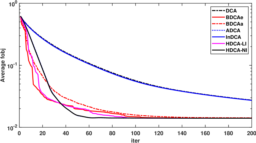
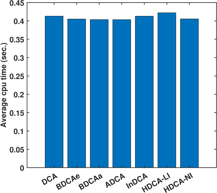
  (a) RAND(10)

  

  

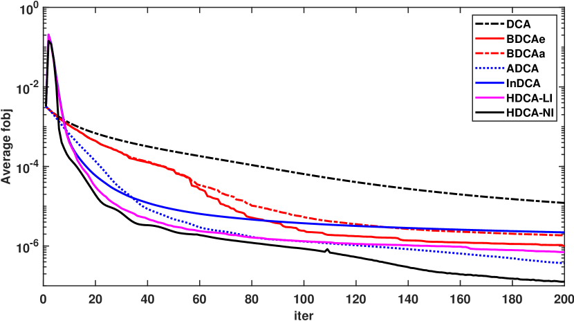
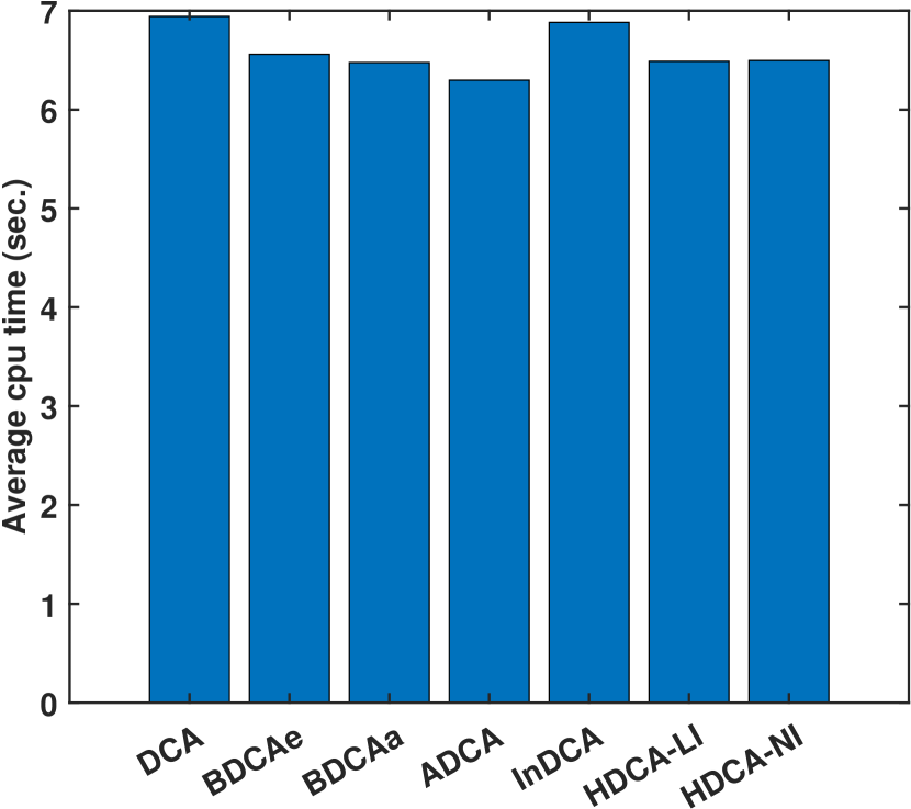
  (b) RAND(100)

  

  

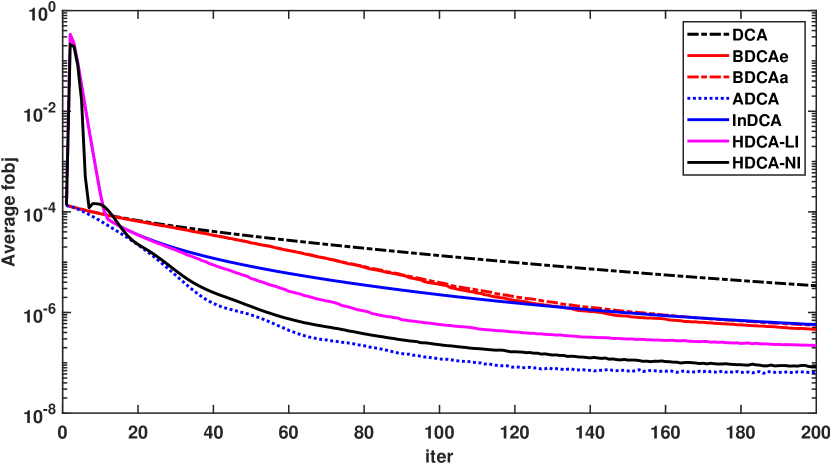
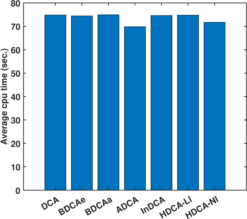
  (c) RAND(500)

  Figure 1. Numerical results of DCA, BDCAe, BDCAa, ADCA, InDCA, HDCA-LI and HDCA-NI for solving (DCP1) on the test datasets RAND(n) with $n\in\{10,100,500\}$.

  • The accelerated variants of DCA (HDCA-NI, HDCA-LI, BDCAe, BDCAa, ADCA, InDCA) consistently outperform the classical DCA.

  • The hybrid method HDCA-NI yields the best numerical result in terms of the average objective value for the majority of tested cases, with the exception on the dataset RAND(500), where ADCA emerges as the best performer.

  • HDCA-LI secures the second-best average objective value for the dataset RAND(10), while ADCA holds the position for the dataset RAND(100).

  • For accelerated DCA without hybridization (i.e., BDCAe, BDCAa, InDCA and ADCA), it appears that ADCA outperforms BDCAe, which in turn outperforms BDCAa, while InDCA ranks as the second-worst algorithm.

  • As anticipated, the average CPU time per iteration remains nearly identical for all tested DCA-type algorithms.

  

  

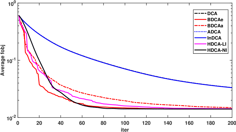
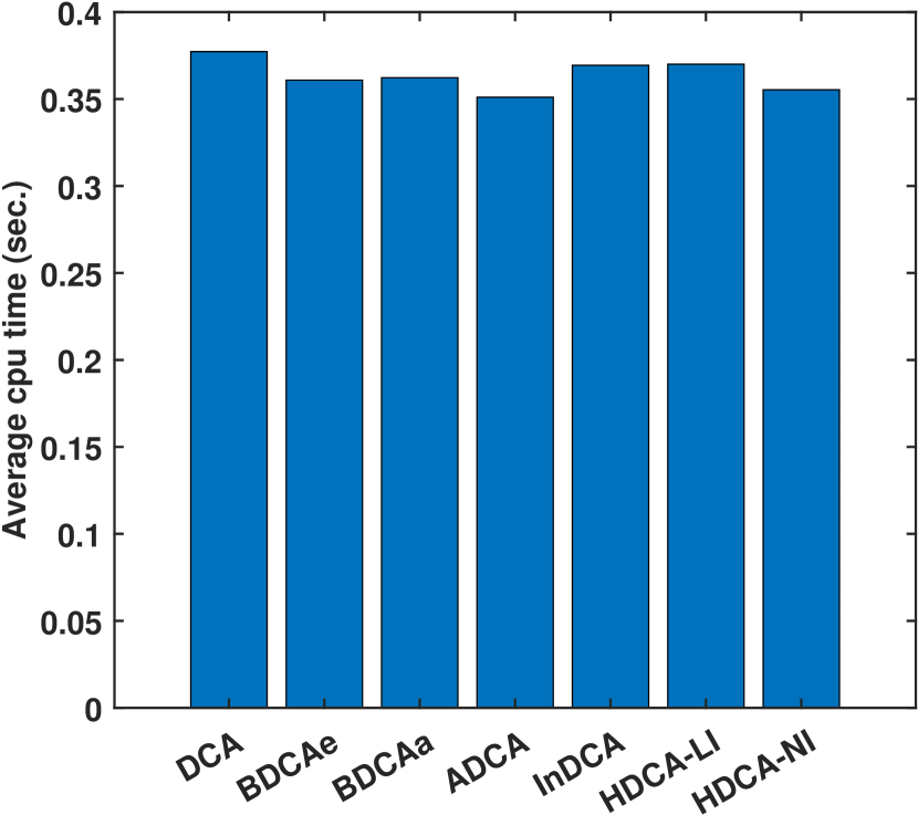
  (a) RAND(10)

  

  

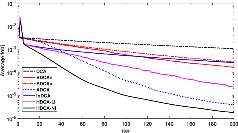
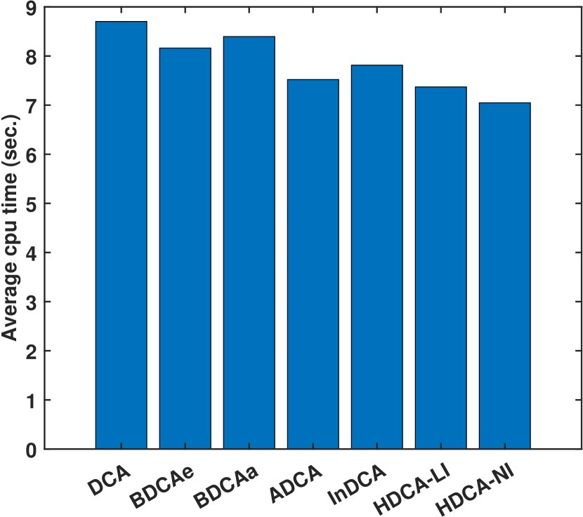
  (b) RAND(100)

  

  

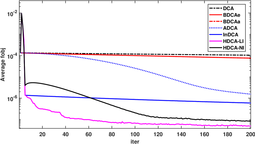
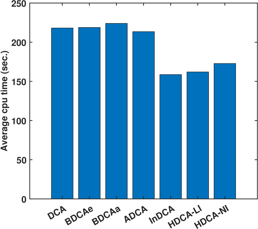
  (c) RAND(500)

  Figure 2. Numerical results of DCA, BDCAe, BDCAa, ADCA, InDCA, HDCA-LI and HDCA-NI for solving (DCP2) on the datasets RAND(n) with $n\in\{10,100,500\}$.

• For (DCP2), we once again observe in Figure 2 that all accelerated variants of DCA outshine the classical DCA in terms of the average objective value. Among the top performers, HDCA-NI, HDCA-LI and ADCA consistently stand out, then followed by BDCAe and BDCAa. The performance of InDCA, however, varies significantly, as illustrated by the contrasting performance of InDCA on RAND(10) and RAND(500), where it performs remarkably on RAND(500) but merely matches the classical DCA on RAND(10).

• 

  

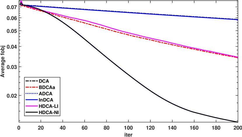
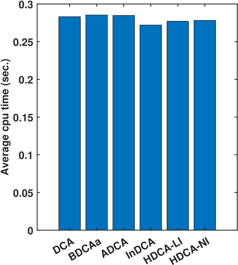
  (a) RAND(10)

  

  

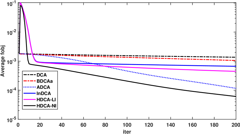
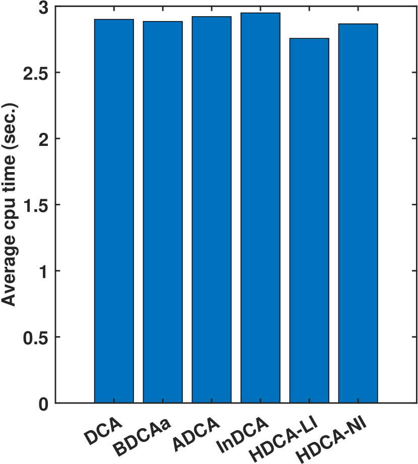
  (b) RAND(100)

  

  

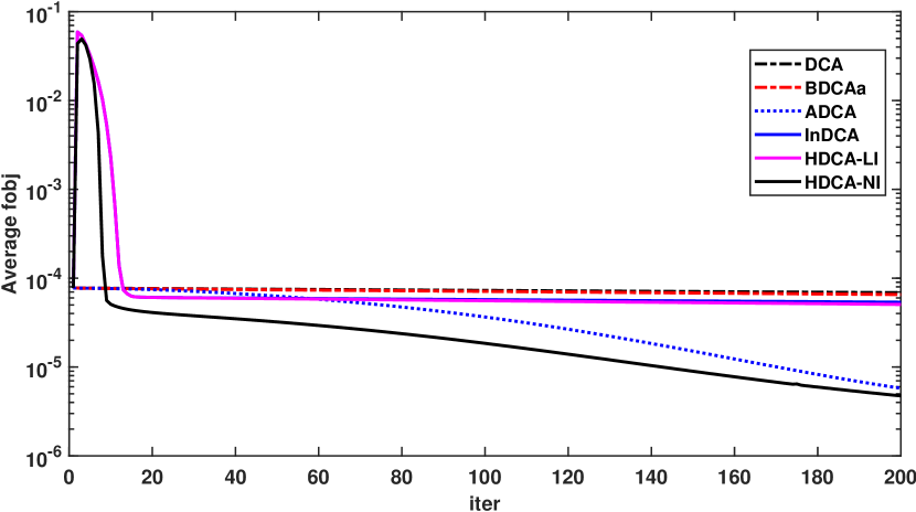
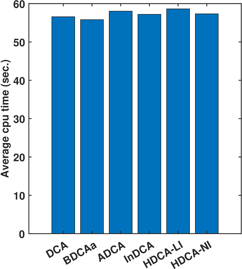
  (c) RAND(500)

  Figure 3. Numerical results of DCA, BDCAa, ADCA, InDCA, HDCA-LI and HDCA-NI for solving (DCP3) on the datasets RAND(n) with $n\in\{10,100,500\}$.

  For (DCP3), we observe a similar result in Figure 3, with all accelerated DCA variants outperforming the classical DCA. The best result is consistently provided by HDCA-NI, followed by ADCA, HDCA-LI, BDCAe, and InDCA. It is worth noting that the choice of parameter $\bar{\alpha}=10$ is a conservative setting; it seems that increasing this value often leads to better numerical results for BDCAe and BDCAa. Figure 4 illustrates an example of the impact of $\bar{\alpha}$ on the computed objective value for BDCAa when solving (DCP3) within 200 iterations on the dataset RAND(100). We observe that the optimal result is achieved with $\bar{\alpha}=200$. Beyond this value, the performance of BDCAa plateaus, as $\bar{\alpha}_{k}<200$ for all $k\in\operatorname{\mathbb{N}}$. Notably, this observation is consistent across all DC formulations.

  

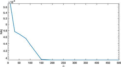
  Figure 4. Example to illustrate the influence of $\bar{\alpha}$ on the objective value for BDCAa.

Tests on the NEP dataset:

The numerical results of the DCA-type algorithms on the NEP dataset are summarized in Tables 2, 3 and 4 for the three DC formulations. In these tables, we adopt the following notations:

• cond($A$) - the condition number of the matrix $A$;

• $f$ - the objective value; The smaller the value of $f$, the higher the quality of the computed solution;

• $c$ - the feasibility measure of the computed solution defined by

  $$c:=-\log(\|[x]_{-}\|+\|[w]_{-}\|+|w^{\top}x|),$$

  where $[x]_{-}=\min\{x,0\}$ and $w=\frac{x^{\top}Ax}{x^{\top}Bx}Bx-Ax$. The larger the value of $c$, the higher the quality of the computed solution;

• avg - average results regarding to $f$ and $c$.

Remark 6.1.

The reasoning behind reporting both $f$ and $c$ is that a small value in $f$ may not necessarily imply a large value in $c$, especially if either the matrix $A$ or $B$ is ill-conditioned. For example, in (DCP1), let’s assume that we obtain an approximate solution $x+\Delta x$ for the exact solution $x$. When the value of $f$ is small, then the error $\Delta x$ is also small. We get from the relation

$$w=\frac{x^{\top}Ax}{x^{\top}Bx}Bx-Ax$$

for the exact solution $(x,w)$ that, if $A$ is ill-conditioned and $B$ is well-conditioned, then $B(x+\Delta x)\approx Bx$ and

$$\frac{(x+\Delta x)^{\top}A(x+\Delta x)}{(x+\Delta x)^{\top}B(x+\Delta x)}B(x+\Delta x)-A(x+\Delta x)\approx w+\underbrace{\frac{2x^{\top}A\Delta x+\Delta x^{\top}A\Delta x}{x^{\top}Bx}Bx-A\Delta x}_{\approx\Delta w}.$$

Consequently, when dealing with an ill-conditioned $A$, we will get a large $A\Delta x$, indicating that $\Delta w$ could be substantial as well. This, in turn, could result in a considerable $\|[w+\Delta w]_{-}\|$ and ultimately lead to a small $c$.

Table 2. Numerical results of DCA, BDCAe, BDCAa, ADCA, InDCA, HDCA-LI and HDCA-NI for solving (DCP1) on the NEP dataset with MaxIT=200.

Prob	cond($A$)	DCA		BDCAe		BDCAa		ADCA		InDCA		HDCA-LI		HDCA-NI
		$f$	$c$	$f$	$c$	$f$	$c$	$f$	$c$	$f$	$c$	$f$	$c$	$f$	$c$
bfw398a	7.58e+03	1.30e-04	1.32	7.86e-05	1.40	1.13e-04	1.34	1.42e-06	2.35	1.88e-06	1.93	8.87e-07	2.20	9.42e-07	2.21
bfw62a	1.48e+03	4.30e-06	1.55	1.57e-06	1.80	3.26e-06	1.61	9.88e-07	2.20	8.85e-07	1.94	6.42e-07	2.10	4.06e-07	2.23
bfw782a	4.62e+03	1.98e-04	0.94	1.27e-04	1.04	1.83e-04	0.96	3.45e-06	2.00	2.77e-06	1.77	1.30e-06	1.89	3.59e-07	2.04
bwm200	2.93e+03	2.21e-08	-2.47	2.09e-08	-2.47	3.08e-08	-2.47	3.07e-08	-2.47	2.35e-08	-2.47	3.03e-08	-2.47	2.01e-08	-2.36
dwa512	3.72e+04	4.65e-04	0.57	2.12e-05	1.02	3.79e-04	0.60	1.94e-06	1.44	2.43e-06	1.42	1.59e-06	1.49	8.21e-08	2.44
dwb512	4.50e+00	3.56e-04	1.65	2.20e-05	2.15	3.53e-04	1.65	7.63e-05	1.91	1.64e-05	2.35	2.34e-06	2.67	1.17e-07	3.01
lop163	3.42e+07	3.06e-04	0.94	4.59e-06	1.92	2.78e-04	0.96	2.42e-06	2.04	3.47e-05	1.58	1.62e-05	1.68	2.98e-07	2.32
mhd416a	2.41e+25	1.80e-09	0.18	4.55e-09	0.18	3.62e-09	0.18	4.56e-09	0.18	8.75e-09	0.24	3.34e-10	0.27	1.67e-08	1.62
mhd416b	5.05e+09	9.55e-08	3.57	9.04e-08	3.57	9.72e-08	3.57	1.20e-07	3.57	5.67e-05	2.57	2.71e-08	5.04	3.29e-09	5.05
odep400a	8.31e+05	3.50e-04	0.10	2.53e-04	0.15	3.35e-04	0.10	1.17e-05	0.74	9.26e-05	0.41	4.41e-05	0.54	2.98e-08	1.97
olm100	2.78e+04	2.00e-08	-1.20	1.65e-08	-1.20	2.82e-08	-1.20	2.38e-08	-1.20	4.31e-08	-1.49	4.42e-08	-1.49	3.41e-08	-1.55
olm500	7.65e+05	1.85e-08	-2.80	3.14e-07	-2.80	2.02e-08	-2.80	1.41e-08	-2.81	2.61e-08	-2.86	4.38e-06	-2.91	1.12e-08	-2.81
rbs480a	1.35e+05	2.74e-08	-1.17	2.83e-08	-1.17	2.84e-08	-1.17	3.10e-08	-1.17	6.81e-08	-2.09	5.38e-08	-2.09	1.48e-08	-1.85
rbs480b	1.63e+05	4.01e-08	-1.57	3.96e-08	-1.57	3.99e-08	-1.57	3.81e-08	-1.57	-4.37e-08	-2.08	3.81e-08	-2.08	9.70e-08	-1.98
rdb200	8.32e+02	1.24e-05	-0.78	1.23e-05	-0.78	1.24e-05	-0.78	1.22e-05	-0.78	3.48e-07	-0.11	2.46e-07	-0.11	2.46e-07	-0.15
rdb450	1.64e+03	2.49e-06	-1.01	2.47e-06	-1.01	2.52e-06	-1.01	2.49e-06	-1.01	8.67e-08	-0.49	8.44e-08	-0.49	1.21e-07	-0.55
rdb968	2.91e+01	9.80e-06	-0.41	8.82e-06	-0.41	9.48e-06	-0.41	7.74e-06	-0.40	3.13e-06	-0.23	2.68e-06	-0.21	3.41e-07	0.05
rw136	1.49e+05	2.96e-05	1.48	2.95e-05	1.48	2.95e-05	1.48	2.77e-05	1.48	2.26e-05	1.68	5.52e-06	1.89	1.29e-06	2.01
rw496	1.14e+10	6.59e-06	1.78	6.62e-06	1.78	7.31e-06	1.78	6.59e-06	1.78	1.99e-05	1.86	3.42e-06	2.13	1.67e-08	2.85
tols340	2.35e+05	2.35e-08	4.44	1.08e-07	0.50	3.22e-08	1.92	5.78e-08	-3.26	1.02e-08	0.97	1.73e-08	0.81	1.57e-08	2.58
tols90	2.49e+04	1.87e-08	-2.05	1.83e-08	-2.05	1.98e-08	-2.05	2.71e-08	-2.05	3.00e-08	-2.29	3.14e-08	-2.28	2.25e-08	-2.31
tub100	2.36e+04	1.54e-08	-2.67	2.17e-08	-2.67	1.24e-08	-2.67	1.41e-08	-2.67	2.51e-08	-2.67	9.46e-09	-2.67	1.90e-08	-2.56
avg		8.49e-05	0.11	2.58e-05	0.04	7.76e-05	0.00	7.06e-06	0.01	1.16e-05	0.09	3.80e-06	0.27	2.05e-07	0.65

Table 3. Numerical results of DCA, BDCAe, BDCAa, ADCA, InDCA, HDCA-LI and HDCA-NI for solving (DCP2) on the NEP dataset with MaxIT=200.

Prob	cond($A$)	DCA		BDCAe		BDCAa		ADCA		InDCA		HDCA-LI		HDCA-NI
		$f$	$c$	$f$	$c$	$f$	$c$	$f$	$c$	$f$	$c$	$f$	$c$	$f$	$c$
bfw398a	7.58e+03	1.73e-04	1.28	1.32e-04	1.32	1.52e-04	1.30	7.13e-06	1.96	1.53e-06	1.99	1.00e-06	2.12	4.40e-07	2.20
bfw62a	1.48e+03	1.59e-06	1.82	2.53e-07	2.31	9.28e-07	1.95	6.10e-07	2.11	3.69e-07	2.24	2.32e-07	2.49	1.49e-07	2.63
bfw782a	4.62e+03	2.33e-04	0.92	1.84e-04	0.98	2.19e-04	0.93	1.92e-05	1.50	2.96e-06	1.83	1.36e-06	1.96	5.71e-07	2.11
bwm200	2.93e+03	3.44e-06	-2.46	3.96e-06	-2.45	3.47e-06	-2.46	4.09e-06	-2.46	3.34e-06	-2.46	4.34e-06	-2.46	2.87e-06	-2.45
dwa512	3.72e+04	5.87e-04	0.55	2.37e-05	1.02	3.74e-04	0.60	3.01e-06	1.35	5.54e-05	0.98	2.08e-05	1.08	5.46e-08	2.14
dwb512	4.50e+00	3.60e-04	1.65	2.25e-05	2.13	3.49e-04	1.65	9.88e-05	1.86	7.15e-05	1.99	2.49e-05	2.16	7.21e-06	2.23
lop163	3.42e+07	3.24e-04	0.93	1.68e-05	1.54	2.56e-04	0.98	3.75e-06	1.91	7.21e-05	1.35	2.79e-05	1.51	1.66e-06	2.09
mhd416a	2.41e+25	1.01e-06	1.00	7.37e-07	1.07	1.02e-06	1.00	1.10e-06	0.98	1.03e-06	0.99	1.04e-06	0.99	3.39e-06	0.74
mhd416b	5.05e+09	1.24e-07	3.57	1.35e-07	3.57	1.29e-07	3.57	1.64e-07	3.57	2.37e-04	1.80	1.33e-07	4.32	6.28e-09	5.42
odep400a	8.31e+05	3.68e-04	0.09	4.16e-05	0.47	3.25e-04	0.11	2.23e-05	0.57	1.76e-04	0.28	4.63e-05	0.50	1.64e-06	1.12
olm100	2.78e+04	9.22e-07	-1.18	1.95e-06	-1.17	9.27e-07	-1.18	1.73e-06	-1.17	2.89e-06	-1.17	2.89e-06	-1.18	3.19e-06	-1.17
olm500	7.65e+05	6.61e-06	-2.85	6.61e-06	-2.85	6.61e-06	-2.85	6.87e-06	-2.85	6.45e-06	-2.85	6.45e-06	-2.85	1.02e-05	-2.89
rbs480a	1.35e+05	-6.50e-07	-1.17	-7.77e-07	-1.16	-1.14e-06	-1.16	-9.94e-07	-1.16	-7.38e-08	-1.18	-7.38e-08	-1.18	-5.44e-07	-1.20
rbs480b	1.63e+05	-1.69e-06	-1.56	-3.85e-07	-1.56	-6.90e-07	-1.55	-8.60e-07	-1.55	-5.78e-07	-1.50	-5.78e-07	-1.50	-9.76e-07	-1.50
rdb200	8.32e+02	1.25e-05	-0.78	1.23e-05	-0.78	1.25e-05	-0.78	1.25e-05	-0.78	1.21e-05	-0.78	1.21e-05	-0.78	1.21e-05	-0.77
rdb450	1.64e+03	2.60e-06	-1.01	2.59e-06	-1.01	2.61e-06	-1.01	2.60e-06	-1.01	2.91e-06	-1.01	2.75e-06	-1.00	3.09e-06	-1.00
rdb968	2.91e+01	9.01e-06	-0.41	8.61e-06	-0.41	8.85e-06	-0.41	8.40e-06	-0.40	6.30e-06	-0.25	4.56e-06	-0.25	4.92e-06	-0.29
rw136	1.49e+05	2.97e-05	1.48	2.95e-05	1.48	2.95e-05	1.48	2.91e-05	1.48	5.22e-05	1.56	2.12e-05	1.62	2.49e-06	1.91
rw496	1.14e+10	6.75e-06	1.78	6.68e-06	1.78	6.67e-06	1.78	6.69e-06	1.78	4.18e-05	1.78	1.77e-05	1.85	7.17e-08	2.77
tols340	2.35e+05	5.10e-05	-0.57	-5.80e-06	-0.61	-8.79e-07	-0.85	1.30e-04	-1.10	5.83e-05	-0.67	-7.83e-06	-0.63	8.72e-05	-1.20
tols90	2.49e+04	2.07e-05	-2.28	2.34e-05	-2.28	1.08e-05	-2.27	2.46e-05	-2.24	1.88e-05	-2.29	2.16e-05	-2.25	2.32e-05	-2.18
tub100	2.36e+04	5.75e-06	-2.66	5.73e-06	-2.66	5.75e-06	-2.66	5.75e-06	-2.66	5.73e-06	-2.66	5.73e-06	-2.66	5.75e-06	-2.66
avg		9.98e-05	-0.08	2.34e-05	0.03	8.01e-05	-0.08	1.76e-05	0.08	3.76e-05	-0.00	9.75e-06	0.18	7.67e-06	0.37

Table 4. Numerical results of DCA, BDCAa, ADCA, InDCA, HDCA-LI and HDCA-NI for solving (DCP3) on the NEP dataset with MaxIT=200.

Prob	cond($A$)	DCA		BDCAa		ADCA		InDCA		HDCA-LI		HDCA-NI
		$f$	$c$	$f$	$c$	$f$	$c$	$f$	$c$	$f$	$c$	$f$	$c$
bfw398a	7.58e+03	1.18e-02	0.85	9.35e-03	0.85	2.03e-03	0.86	1.18e-02	0.85	9.24e-03	0.85	2.02e-03	0.86
bfw62a	1.48e+03	5.22e-03	0.78	1.54e-03	0.79	7.53e-04	0.88	4.98e-03	0.78	1.54e-03	0.79	7.65e-04	0.87
bfw782a	4.62e+03	1.36e-03	0.88	1.21e-03	0.88	6.29e-04	0.88	1.34e-03	0.88	1.24e-03	0.88	6.22e-04	0.88
bwm200	2.93e+03	1.39e-08	-2.47	1.38e-08	-2.47	1.69e-08	-2.47	1.40e-08	-2.47	1.38e-08	-2.47	1.25e-08	-2.31
dwa512	3.72e+04	2.16e-05	0.97	2.15e-05	0.97	2.15e-05	0.97	2.13e-05	0.98	2.15e-05	0.97	2.13e-05	0.98
dwb512	4.50e+00	3.74e-05	1.99	3.73e-05	1.99	3.75e-05	1.99	3.74e-05	1.99	3.78e-05	1.99	3.77e-05	1.99
lop163	3.42e+07	1.75e-04	0.94	1.65e-04	0.95	8.51e-05	1.03	1.72e-04	0.95	1.61e-04	0.96	8.27e-05	1.04
mhd416a	2.41e+25	4.30e-09	0.70	3.58e-09	0.70	1.36e-08	0.70	2.41e-08	0.23	3.18e-09	0.70	2.70e-11	-0.09
mhd416b	5.05e+09	9.95e-06	2.54	1.01e-05	2.54	1.01e-05	2.54	1.07e-05	2.54	1.04e-05	2.54	1.09e-05	2.54
odep400a	8.31e+05	9.86e-05	0.30	9.84e-05	0.30	5.28e-05	0.44	9.81e-05	0.30	9.81e-05	0.30	4.23e-05	0.48
olm100	2.78e+04	4.58e-09	-1.20	1.34e-08	-1.20	4.43e-09	-1.20	3.28e-09	-1.44	1.51e-08	-1.16	3.38e-09	-1.51
olm500	7.65e+05	1.44e-08	-2.81	1.82e-08	-2.81	1.28e-08	-2.81	9.81e-09	-2.82	2.04e-08	-2.66	1.52e-08	-2.78
rbs480a	1.35e+05	1.70e-08	-1.95	2.31e-08	-1.95	1.46e-08	-1.95	2.04e-08	-2.09	2.42e-08	-1.89	1.43e-08	-2.00
rbs480b	1.63e+05	3.55e-08	-2.01	2.05e-08	-2.01	2.41e-08	-2.01	3.11e-08	-2.08	1.99e-08	-1.95	1.82e-08	-2.01
rdb200	8.32e+02	4.97e-07	-0.49	5.00e-07	-0.49	5.12e-07	-0.49	7.61e-07	-0.33	5.77e-07	-0.49	4.79e-07	-0.18
rdb450	1.64e+03	2.11e-07	-0.86	2.16e-07	-0.86	2.22e-07	-0.86	1.95e-07	-0.74	2.95e-07	-0.85	9.34e-08	-0.59
rdb968	2.91e+01	5.61e-06	-0.47	5.62e-06	-0.47	4.80e-06	-0.44	5.37e-06	-0.46	5.61e-06	-0.47	3.48e-06	-0.37
rw136	1.49e+05	2.79e-04	0.84	2.73e-04	0.84	2.03e-04	0.90	2.72e-04	0.84	2.67e-04	0.84	1.97e-04	0.91
rw496	1.14e+10	1.85e-04	0.89	1.85e-04	0.89	1.67e-04	0.91	1.83e-04	0.89	1.81e-04	0.90	1.65e-04	0.92
tols340	2.35e+05	4.18e-08	4.79	4.81e-08	4.76	5.42e-09	5.26	2.00e-09	-2.90	1.46e-08	-0.48	2.13e-09	-2.85
tols90	2.49e+04	1.15e-08	-2.05	9.65e-09	-2.05	2.25e-08	-2.05	5.14e-09	-2.27	4.66e-09	-2.05	2.06e-08	-2.31
tub100	2.36e+04	5.71e-09	-2.67	4.84e-09	-2.67	5.57e-09	-2.67	9.87e-09	-2.67	5.16e-09	-2.67	3.54e-09	-2.50
avg		8.73e-04	-0.02	5.86e-04	-0.02	1.81e-04	0.02	8.59e-04	-0.41	5.82e-04	-0.25	1.81e-04	-0.36

Table 5. Numerical results of InDCA, HDCA-LI and HDCA-NI using the conservative inertial strategy for solving (DCP3) on the NEP dataset with MaxIT=200.

Prob	cond($A$)	InDCA		HDCA-LI		HDCA-NI
		$f$	$c$	$f$	$c$	$f$	$c$
bfw398a	7.58e+03	1.18e-02	0.85	9.29e-03	0.85	2.03e-03	0.86
bfw62a	1.48e+03	5.21e-03	0.78	1.72e-03	0.79	7.54e-04	0.88
bfw782a	4.62e+03	1.36e-03	0.87	1.20e-03	0.88	6.27e-04	0.88
bwm200	2.93e+03	1.37e-08	-2.47	1.45e-08	-2.47	3.25e-08	-2.47
dwa512	3.72e+04	2.16e-05	0.97	2.15e-05	0.97	2.15e-05	0.97
dwb512	4.50e+00	3.74e-05	1.99	3.76e-05	1.99	3.76e-05	1.99
lop163	3.42e+07	1.75e-04	0.94	1.63e-04	0.95	8.48e-05	1.03
mhd416a	2.41e+25	5.16e-09	0.70	5.49e-09	0.70	1.41e-08	0.70
mhd416b	5.05e+09	1.06e-05	2.54	9.73e-06	2.54	1.04e-05	2.54
odep400a	8.31e+05	9.87e-05	0.30	9.67e-05	0.30	5.29e-05	0.44
olm100	2.78e+04	1.74e-08	-1.20	1.75e-08	-1.20	1.31e-08	-1.20
olm500	7.65e+05	2.24e-08	-2.81	1.78e-08	-2.81	4.75e-07	-2.81
rbs480a	1.35e+05	2.78e-08	-1.95	1.48e-08	-1.95	1.85e-08	-1.95
rbs480b	1.63e+05	2.38e-08	-2.01	1.92e-08	-2.01	3.15e-08	-2.01
rdb200	8.32e+02	5.04e-07	-0.49	5.00e-07	-0.49	5.13e-07	-0.49
rdb450	1.64e+03	2.15e-07	-0.86	2.13e-07	-0.86	2.17e-07	-0.86
rdb968	2.91e+01	5.61e-06	-0.47	5.61e-06	-0.47	4.81e-06	-0.43
rw136	1.49e+05	2.79e-04	0.84	2.72e-04	0.84	2.02e-04	0.90
rw496	1.14e+10	1.85e-04	0.89	1.85e-04	0.89	1.69e-04	0.91
tols340	2.35e+05	1.50e-07	4.57	8.07e-09	5.06	5.21e-08	4.76
tols90	2.49e+04	1.76e-08	-2.05	7.84e-09	-2.05	2.14e-08	-2.05
tub100	2.36e+04	5.37e-09	-2.67	5.73e-09	-2.67	5.49e-09	-2.67
avg		8.73e-04	-0.03	5.91e-04	-0.01	1.82e-04	-0.00

As seen in Table 2 for (DCP1), the best average value in $f$ is achieved by HDCA-NI, followed by HDCA-LI, InDCA, BDCAe, BDCAa, and DCA. The best average value in $c$ is also obtained by HDCA-NI, with the subsequent ranking being HDCA-LI, DCA, InDCA, BDCAe, ADCA, and BDCAa. Similar results are observed in Table 3 for (DCP2). It is worth noting that the inertial-based methods (InDCA, HDCA-LI, and HDCA-NI) perform poorly for (DCP3) when $A$ is ill-conditioned, as seen in Table 4. For example, in the case tols340 where cond($A$)=2.35e+05, the value of $c$ is $-2.85$ for HDCA-NI, $-2.90$ for InDCA, $-0.48$ for HDCA-BI, $4.79$ for DCA, $4.76$ for BDCAa, and $5.26$ for ADCA. To some extent, this can be alleviated by using a ‘conservative’ inertial strategy, which introduces the inertial force $\gamma(x^{k}-x^{k-1})$ when $k\geq 2$ instead of $k\geq 0$. Then, we will get improvement in $c$ as $4.57$ for InDCA, $5.00$ for HDCA-LI, and $4.76$ for HDCA-NI. The numerical results of InDCA, HDCA-LI, and HDCA-NI using the conservative inertial strategy are summarized in Table 5, and we can observe that the average value of $c$ is greatly improved at the cost of a slight increase in the average value of $f$.

We conclude that the best DCA-type algorithm is always given by HDCA-NI, hence in the next subsection, we will compare it with other optimization solvers.

6.2. Numerical results of other optimization solvers

In this section, we present the numerical results of the optimization solvers IPOPT, KNITRO, and FILTERSD in comparison with HDCA-NI. Our primary focus is to evaluate their performance based on the objective value $f$, the feasibility measure $c$, and the CPU time (in seconds). To determine the CPU time for HDCA-NI, we employ the following stopping criteria:

$$|f^{k+1}-f^{k}|\leq(1+|f^{k+1}|)\varepsilon,$$

where the tolerance $\varepsilon$ is set to $10^{-8}$, and $f^{k}$ represents the objective value at the $k$-th iteration. The other solvers use their default termination settings. The numerical results for solving (NLP1),(NLP2), and (NLP3) are summarized in Tables 6, 7 and 8, respectively. Furthermore, instead of providing the results for all $10$ instances within each dataset RAND(n), we only present their averages.

• For the results of (NLP1) in Table 6, we observe that IPOPT performs best in terms of average values for $f$, $c$, and CPU time. HDCA-NI is the second-best method, followed by KNITRO and FILTERSD. It is important to note that, in contrast to IPOPT, FILTERSD and HDCA-NI, the solver KNITRO demonstrates considerable instability and frequently encounters “LCP solver problem” issues, in ill-conditioned NEP instances. This results in significantly different outcomes in each run. Therefore, we consider the best result for FILTERSD in terms of $f$ across three runs. Nevertheless, FILTERSD still exhibits poor performance in terms of average $f$, $c$, and CPU time.

• For the results of (NLP2) in Table 7 and (NLP3) in Table 8, IPOPT remains the best solver in terms of average $f$, $c$, and CPU time. HDCA-NI often yields good average values for $f$, but with poor average values for $c$. FILTERSD consistently provides the worst results for $f$.

Table 6. Numerical results of IPOPT, KNITRO, FILTERSD and HDCA-NI for solving (NLP1) on RAND(n) and NEP datasets.

Dataset	HDCA-NI			IPOPT			KNITRO			FILTERSD
	$f$	$c$	CPU	$f$	$c$	CPU	$f$	$c$	CPU	$f$	$c$	CPU
RAND(10)	1.40e-02	1.88	0.451	4.71e-03	6.19	0.022	9.14e-03	4.17	0.008	3.79e-03	3.17	0.006
RAND(100)	1.41e-03	1.03	2.793	4.71e-04	3.45	0.816	9.15e-04	2.32	1.646	2.81e+01	0.15	0.670
RAND(500)	1.41e-04	0.55	28.157	4.79e-05	1.50	5.854	6.61e-04	0.37	17.710	5.69e+03	-0.39	32.241
bfw398a	1.39e-06	2.14	8.173	1.68e-05	2.88	0.428	1.82e-03	1.39	0.856	6.08e+01	1.27	1.839
bfw62a	6.42e-07	2.03	0.533	3.82e-10	4.54	0.315	8.43e-07	2.52	0.602	1.88e-07	2.09	0.659
bfw782a	1.00e-06	1.86	11.712	3.36e-05	2.65	0.492	7.20e-04	1.16	6.106	1.25e+02	1.38	6.422
bwm200	1.07e-08	-2.45	0.408	3.98e-08	-0.79	0.029	5.50e-06	-2.01	0.855	3.13e+01	-1.23	0.091
dwa512	8.78e-07	1.74	4.129	1.69e-08	2.73	0.840	1.00e-04	1.93	2.908	8.21e-04	0.50	68.637
dwb512	2.50e-07	2.91	4.415	3.83e-08	3.60	0.647	1.85e-05	2.18	9.078	3.75e-04	1.65	4.769
lop163	6.59e-07	2.15	6.083	6.42e-13	4.99	0.790	8.13e-07	2.35	0.256	4.03e-04	0.89	2.824
mhd416a	-1.29e-09	1.67	0.256	1.10e-07	-1.11	0.092	1.75e-04	-0.46	6.693	6.57e+01	-0.37	0.787
mhd416b	2.06e-07	3.12	3.537	4.52e-07	3.42	0.681	1.51e-03	1.89	0.936	6.85e+01	1.79	0.522
odep400a	2.91e-07	1.54	4.077	3.71e-08	3.14	0.290	8.27e-05	1.78	1.087	4.16e-04	0.07	25.959
olm100	2.82e-09	-1.55	0.115	3.48e-09	-0.88	0.022	1.63e-05	-0.88	0.111	1.24e-09	-1.41	0.053
olm500	-5.14e-08	-2.91	3.567	1.62e-06	-1.73	0.081	1.10e-03	-2.11	14.042	1.03e-10	-3.68	18.787
rbs480a	2.52e-08	-1.92	2.548	7.03e-08	-0.73	0.455	1.17e-03	-0.72	6.043	8.18e+01	-0.85	6.370
rbs480b	2.40e-08	-2.03	1.933	8.32e-08	-1.17	0.719	1.18e-03	-1.19	6.771	4.79e+04	-2.01	25.796
rdb200	2.81e-07	-0.15	0.502	1.57e-08	0.30	0.125	1.61e-05	-0.75	0.413	5.78e+03	-0.79	0.187
rdb450	1.33e-07	-0.53	0.681	1.54e-08	0.50	0.065	5.00e-04	0.38	1.977	1.84e+04	-0.99	1.954
rdb968	4.46e-06	-0.28	2.027	8.28e-08	1.58	0.324	3.35e-04	1.19	18.358	1.43e+02	0.70	11.839
rw136	1.43e-06	2.00	4.554	1.54e-13	5.32	0.865	1.78e-07	2.57	4.571	2.97e-05	1.48	1.797
rw496	3.06e-07	2.27	5.993	1.44e-08	4.85	0.360	3.00e-05	2.22	3.469	6.60e-06	1.77	4.325
tols340	2.87e-06	-0.03	1.918	6.85e-06	-2.29	0.064	1.39e-03	-2.80	4.342	2.09e-01	-2.09	1.808
tols90	3.51e-09	-2.32	0.086	1.68e-07	-2.04	0.036	4.36e-05	-2.19	0.257	1.25e-15	-0.34	0.161
tub100	4.56e-09	-2.64	0.267	2.85e-08	-1.75	0.018	4.36e-07	-1.73	0.149	4.02e-09	-2.62	0.057
avg	6.24e-06	0.29	3.827	4.32e-06	1.18	0.544	4.35e-04	0.28	4.304	3.13e+03	-0.13	8.715

Table 7. Numerical results of IPOPT, KNITRO, FILTERSD and HDCA-NI for solving (NLP2) on RAND(n) and NEP datasets.

Dataset	HDCA-NI			IPOPT			KNITRO			FILTERSD
	$f$	$c$	CPU	$f$	$c$	CPU	$f$	$c$	CPU	$f$	$c$	CPU
RAND(10)	1.41e-02	2.00	0.594	3.27e-03	6.13	0.025	5.66e-03	5.13	0.009	6.95e-03	2.98	0.023
RAND(100)	1.41e-03	0.99	5.435	3.27e-04	3.19	0.726	5.66e-04	2.36	0.813	1.06e+01	0.13	0.780
RAND(500)	1.45e-04	0.24	30.844	3.36e-05	1.48	8.736	1.44e-03	0.48	3.801	1.35e+02	-0.21	6.294
bfw398a	9.86e-07	2.08	4.710	1.88e-08	3.63	2.405	8.69e-06	1.92	1.078	5.97e+01	1.27	0.850
bfw62a	9.22e-06	1.64	0.113	1.24e-08	3.52	0.230	1.88e-06	2.18	0.157	1.30e-06	1.95	0.764
bfw782a	1.53e-06	1.88	8.884	2.24e-05	2.73	1.318	5.85e-04	1.35	1.281	1.24e+02	1.38	6.211
bwm200	6.33e-08	-2.47	0.105	3.98e-08	-0.78	0.033	1.19e-05	-0.66	0.063	-1.23e+03	-1.23	0.082
dwa512	3.72e-07	1.79	2.908	1.70e-08	2.72	0.736	7.13e-04	1.98	0.411	8.21e-04	0.50	3.533
dwb512	1.70e-05	2.08	1.275	1.22e-07	3.45	1.051	1.60e-05	2.17	1.924	3.12e-08	3.59	33.208
lop163	3.48e-06	1.90	3.343	-7.70e-09	4.40	0.314	2.07e-03	1.93	0.030	4.03e-04	0.89	0.105
mhd416a	1.52e-08	2.99	0.142	1.10e-07	-0.07	0.091	3.23e-04	-0.55	0.202	-1.20e+03	-0.37	0.594
mhd416b	3.19e-07	2.63	2.249	9.96e-08	3.54	0.698	1.01e-05	2.35	1.132	6.79e+01	1.79	0.296
odep400a	1.54e-06	1.13	5.524	5.02e-09	3.30	0.605	8.33e-04	1.58	0.207	5.41e-08	1.81	23.659
olm100	8.65e-07	-1.17	0.206	2.48e-09	-1.03	0.026	3.63e-07	-0.82	0.017	1.98e-07	-2.24	0.040
olm500	8.16e-06	-2.88	1.119	1.62e-06	-1.38	0.077	5.00e-04	-1.60	0.425	-4.19e-12	-2.92	7.570
rbs480a	-8.66e-07	-1.20	17.931	7.02e-08	-0.61	0.313	7.25e-04	-0.73	0.311	-4.12e+02	-0.85	3.955
rbs480b	-4.15e-07	-1.50	8.610	4.66e-06	-1.18	0.845	1.29e-05	-1.15	0.478	-3.42e+02	-1.15	8.460
rdb200	1.23e-05	-0.78	1.111	6.56e-08	0.35	0.085	9.03e-07	0.31	0.050	7.25e-06	-0.67	0.323
rdb450	3.01e-06	-1.01	0.443	1.53e-08	0.49	0.078	9.54e-05	0.05	0.380	4.78e+04	-1.23	2.466
rdb968	5.36e-06	-0.29	24.240	8.22e-08	1.88	0.435	2.96e-04	1.46	1.914	1.20e+02	0.70	14.062
rw136	8.37e-06	1.66	2.067	-8.18e-09	4.40	0.487	1.26e-07	4.43	1.682	5.27e-07	2.18	1.883
rw496	3.57e-07	2.44	9.305	5.18e-06	3.68	0.322	2.80e-06	2.38	0.984	8.31e-08	2.56	47.600
tols340	1.15e-04	-2.31	17.904	6.86e-06	-2.85	0.049	8.59e-04	-2.55	0.217	2.20e-11	8.92	3.339
tols90	5.37e-06	-2.15	28.596	1.68e-07	-2.09	0.025	2.87e-05	-2.16	0.015	4.58e-09	-2.03	0.047
tub100	5.70e-06	-2.66	0.590	2.78e-08	-1.50	0.022	3.23e-06	-1.07	0.015	1.11e-09	-2.31	0.045
avg	1.37e-05	0.16	6.889	3.01e-06	1.12	0.759	3.41e-04	0.53	0.671	1.80e+03	0.49	6.615

Table 8. Numerical results of IPOPT, KNITRO, FILTERSD and HDCA-NI for solving (NLP3) on RAND(n) and NEP datasets.

Dataset	HDCA-NI			IPOPT			KNITRO			FILTERSD
	$f$	$c$	CPU	$f$	$c$	CPU	$f$	$c$	CPU	$f$	$c$	CPU
RAND(10)	6.86e-03	1.43	0.753	4.57e-03	6.23	0.018	4.72e-03	5.18	0.015	6.39e-03	2.41	0.008
RAND(100)	6.99e-04	0.62	3.267	4.57e-04	3.64	0.774	4.73e-04	3.11	1.606	3.02e+00	0.56	1.289
RAND(500)	7.37e-05	0.13	47.000	4.59e-05	1.60	6.789	4.73e-05	1.49	91.480	4.07e+01	-0.63	36.676
bfw398a	4.66e-04	0.87	9.086	4.64e-07	3.30	1.639	2.67e-07	3.17	37.139	5.43e+01	1.27	0.756
bfw62a	4.27e-05	1.51	3.626	1.92e-11	4.75	0.352	1.97e-06	2.24	2.598	4.02e-13	5.09	0.014
bfw782a	3.99e-04	0.89	13.881	4.05e-06	3.04	0.684	5.09e-08	3.54	120.165	1.11e+02	1.38	10.282
bwm200	4.78e-09	-2.41	0.074	3.95e-08	-0.26	0.028	1.78e-09	-2.09	0.505	3.68e-10	-1.94	0.352
dwa512	2.12e-05	0.98	0.580	1.02e-08	2.76	0.442	1.02e-07	2.43	370.415	5.61e-07	1.63	53.139
dwb512	3.74e-05	1.99	0.352	8.23e-07	3.23	0.307	1.84e-07	3.36	51.577	1.65e-05	2.06	57.646
lop163	5.15e-05	1.11	2.869	2.50e-12	4.74	0.611	1.20e-08	2.91	0.960	1.13e-05	1.40	2.412
mhd416a	5.23e-11	-0.01	0.149	1.06e-07	-0.54	0.076	9.23e-09	-0.17	3.203	5.76e+01	-0.37	1.237
mhd416b	1.01e-05	2.54	0.347	3.14e-08	3.87	0.284	6.63e-07	3.23	669.339	3.08e-06	2.75	2.933
odep400a	4.77e-05	0.46	2.541	3.80e-08	3.13	0.230	8.18e-08	1.90	17.341	7.84e-07	1.19	27.961
olm100	4.05e-08	-1.51	0.044	2.04e-09	-0.62	0.020	8.10e-08	-0.92	0.117	1.17e-10	-1.04	0.045
olm500	3.21e-08	-2.80	0.321	1.62e-06	-1.91	0.091	1.71e-05	-1.78	12.095	3.12e+03	-2.96	3.099
rbs480a	9.96e-09	-2.04	0.972	6.70e-08	-0.79	0.415	1.51e-05	-0.68	6.660	7.39e+01	-0.85	2.929
rbs480b	8.31e-09	-2.03	1.041	7.88e-08	-1.15	0.509	1.26e-05	-1.18	7.049	9.45e+01	-1.15	10.893
rdb200	5.54e-07	-0.20	0.176	1.11e-08	0.32	0.152	8.26e-08	0.17	0.275	2.94e+01	0.16	0.168
rdb450	1.02e-07	-0.62	0.288	1.27e-04	0.51	0.364	5.96e-06	0.40	2.293	6.48e+01	0.17	1.605
rdb968	3.49e-06	-0.37	1.896	6.32e-08	1.91	0.431	4.14e-06	1.08	17.603	1.28e+02	0.70	17.414
rw136	2.47e-05	1.30	4.793	1.58e-14	5.99	0.645	4.88e-08	2.60	4.538	1.31e-06	1.92	1.696
rw496	1.83e-04	0.89	1.213	7.88e-09	4.59	0.533	1.06e-08	3.03	12.119	1.56e-10	3.75	45.088
tols340	8.53e-10	-2.91	0.148	6.85e-06	-3.02	0.054	2.35e-04	-2.79	3.484	3.50e+04	-0.30	0.995
tols90	6.20e-09	-2.32	0.090	1.68e-07	-1.90	0.026	1.52e-04	-2.11	0.294	2.13e-14	-0.82	0.113
tub100	1.62e-10	-2.57	0.061	2.76e-08	-1.21	0.018	2.44e-09	-2.47	0.081	9.34e-10	-2.39	0.046
avg	5.44e-05	-0.28	3.662	7.49e-06	1.29	0.588	1.97e-05	0.69	57.253	1.55e+03	0.44	11.100

In conclusion, the best optimization solver for all NLP formulations of (AEiCP) among all compared methods is IPOPT. HDCA-NI is competitive with IPOPT and outperforms KNITRO and FILTERSD in terms of the objective value.

7. Conclusions

In this paper, we established three DC programming formulations of (AEiCP) based on the DC-SOS decomposition, which are numerically solved via several accelerated DC programming approaches, including BDCA with exact and inexact line search, ADCA, InDCA and two proposed novel hybrid accelerated DCA (HDCA-LI and HDCA-NI). Numerical simulations were carried out to compare the performance of the proposed DCA-type algorithms against the cutting-edge optimization solvers (IPOPT, KNITRO and FILTERSD). Numerical results indicated noteworthy performance, even on large-scale and ill-conditioned datasets.

Future work will prioritize multiple avenues for enhancement. We aim to refine these DCA-type algorithms to improve the quality of computed results in terms of $c$. A particular focus will be on improving the initialization process, possibly through insightful heuristics, to increase efficiency, especially for large-scale and ill-conditioned instances. Moreover, designing a more efficient algorithm to address the QP formulations of convex subproblems required in all DCA-type methods, instead of relying on a general QP solver will also be a key aspect of our upcoming research efforts.

References

- [1] Samir Adly and Alberto Seeger, A nonsmooth algorithm for cone-constrained eigenvalue problems, Computational Optimization and Applications 49 (2011), no. 2, 299–318.
- [2] Mosek ApS, Mosek optimization toolbox for matlab, User’s Guide and Reference Manual, Version 4 (2019).
- [3] Francisco J Aragón Artacho, Ronan MT Fleming, and Phan T Vuong, Accelerating the dc algorithm for smooth functions, Mathematical Programming 169 (2018), no. 1, 95–118.
- [4] Hedy Attouch, Jérôme Bolte, and Benar Fux Svaiter, Convergence of descent methods for semi-algebraic and tame problems: proximal algorithms, forward–backward splitting, and regularized gauss–seidel methods, Mathematical Programming 137 (2013), no. 1, 91–129.
- [5] Jérôme Bolte, Aris Daniilidis, and Adrian Lewis, The Łojasiewicz inequality for nonsmooth subanalytic functions with applications to subgradient dynamical systems, SIAM Journal on Optimization 17 (2007), no. 4, 1205–1223.
- [6] C. P. Brás, A. Fischer, J. J. Júdice, K. Schönefeld, and S. Seifert, A block active set algorithm with spectral choice line search for the symmetric eigenvalue complementarity problem, Applied Mathematics and Computation 294 (2017), 36–48.
- [7] C. P. Brás, M. Fukushima, J. J. Júdice, and S. Rosa, Variational inequality formulation for the asymmetric eigenvalue complementarity problem and its solution by means of a gap function, Pacific Journal of Optimization 8 (2012), 197–215.
- [8] Richard H Byrd, Jorge Nocedal, and Richard A Waltz, Knitro: An integrated package for nonlinear optimization, Large-scale nonlinear optimization, Springer, 2006, pp. 35–59.
- [9] Welington De Oliveira and Michel P. Tcheou, An inertial algorithm for dc programming, Set-Valued and Variational Analysis 27 (2019), 895–919.
- [10] Francisco Facchinei and Jong-Shi Pang, Finite-dimensional variational inequalities and complementarity problems, Springer, 2003.
- [11] Luís M Fernandes, Joaquim J Júdice, Hanif D Sherali, and Masao Fukushima, On the computation of all eigenvalues for the eigenvalue complementarity problem, Journal of Global Optimization 59 (2014), 307–326.
- [12] Rafael Fernandes, Joaquim Júdice, and Vilmar Trevisan, Complementary eigenvalues of graphs, Linear Algebra and its Applications 527 (2017), 216–231.
- [13] Roger Fletcher and Frank E. Curtis, Filtersd – a library for nonlinear optimization written in fortran.
- [14] IBM, Ibm ilog cplex optimization studio 12.7.
- [15] Alfredo N Iusem, Joaquim Júdice, Valentina Sessa, and Paula Sarabando, Splitting methods for the eigenvalue complementarity problem, Optimization Methods and Software 34 (2019), no. 6, 1184–1212.
- [16] Joaquim Júdice, Masao Fukushima, Alfredo Iusem, José Mario Martinez, and Valentina Sessa, An alternating direction method of multipliers for the eigenvalue complementarity problem, Optimization Methods and Software 36 (2021), no. 2-3, 337–370.
- [17] Joaquim Júdice, Marcos Raydan, Silvério S Rosa, and Sandra A Santos, On the solution of the symmetric eigenvalue complementarity problem by the spectral projected gradient algorithm, Numerical Algorithms 47 (2008), 391–407.
- [18] Joaquim Júdice, Valentina Sessa, and Masao Fukushima, Solution of fractional quadratic programs on the simplex and application to the eigenvalue complementarity problem, Journal of Optimization Theory and Applications 193 (2022), no. 1-3, 545–573.
- [19] Joaquim Júdice, Hanif D. Sherali, Isabel M. Ribeiro, and Silvério S. Rosa, On the asymmetric eigenvalue complementarity problem, Optimization Methods and Software 24 (2009), no. 4-5, 549–568.
- [20] Krzysztof Kurdyka, On gradients of functions definable in o-minimal structures, Annales de l’institut Fourier, vol. 48, 1998, pp. 769–783.
- [21] Hoai An Le Thi, Van Ngai Huynh, and Dinh Tao Pham, Convergence analysis of difference-of-convex algorithm with subanalytic data, Journal of Optimization Theory and Applications 179 (2018), no. 1, 103–126.
- [22] Hoai An Le Thi and Dinh Tao Pham, Dc programming and dca: thirty years of developments, Math. Program., Special Issue dedicated to : DC Programming - Theory, Algorithms and Applications 169 (2018), no. 1, 5–68.
- [23] Yi-Shuai Niu, On difference-of-sos and difference-of-convex-sos decompositions for polynomials, arXiv:1803.09900 (2018).
- [24] by same author, On the convergence analysis of dca, arXiv:2211.10942 (2022).
- [25] by same author, An accelerated dc programming approach with exact line search for the symmetric eigenvalue complementarity problem, arXiv:2301.09098 (2023).
- [26] Yi-Shuai Niu, Joaquim Júdice, Hoai An Le Thi, and Dinh Tao Pham, Solving the quadratic eigenvalue complementarity problem by dc programming, Modelling, Computation and Optimization in Information Systems and Management Sciences, Advances in Intelligent Systems and Computing 359 (2015), 203–214.
- [27] by same author, Improved dc programming approaches for solving the quadratic eigenvalue complementarity problem, Applied Mathematics and Computation 353 (2019), 95–113.
- [28] Yi-Shuai Niu, Hoai An Le Thi, Dinh Tao Pham, and Joaquim Júdice, Efficient dc programming approaches for the asymmetric eigenvalue complementarity problem, Optimization Methods and Software 28 (2013), 812–829.
- [29] Yi-Shuai Niu, Ya-Juan Wang, Hoai An Le Thi, and Dinh Tao Pham, High-order moment portfolio optimization via an accelerated difference-of-convex programming approach and sums-of-squares, arXiv:1906.01509 (2019).
- [30] Jorge Nocedal and Stephen J. Wright, Numerical optimization, Spinger, 2006.
- [31] Gurobi Optimization, Gurobi 7.0.
- [32] Dinh Tao Pham and Hoai An Le Thi, Convex analysis approach to d.c. programming: theory, algorithms and applications, Acta Math. Vietnam. 22 (1997), no. 1, 289–355. MR 1479751
- [33] by same author, Dc optimization algorithms for solving the trust region subproblem, SIAM Journal on Optimization 8 (1998), 476–507.
- [34] by same author, The dc programming and dca revisited with dc models of real world nonconvex optimization problems, Annals of Operations Research 133 (2005), 23–46.
- [35] Dinh Tao Pham and El Bernoussi Souad, Algorithms for solving a class of nonconvex optimization problems. methods of subgradients, Fermat days 85: Mathematics for Optimization, North-Holland Mathematics Studies, vol. 129, Elsevier, 1986, pp. 249–271.
- [36] Duy Nhat Phan, Hoai Minh Le, and Hoai An Le Thi, Accelerated difference of convex functions algorithm and its application to sparse binary logistic regression, IJCAI, 2018, pp. 1369–1375.
- [37] Duy Nhat Phan and Hoai An Le Thi, Dca based algorithm with extrapolation for nonconvex nonsmooth optimization, arXiv preprint arXiv:2106.04743 (2021).
- [38] António Pinto Da Costa, Isabel Narra Figueiredo, Joaquim Júdice, and J. A. C. Martins, A complementarity eigenproblem in the stability analysis of finite dimensional elastic systems with frictional contact, Complementarity: applications, algorithms and extensions, Springer, 2001, pp. 67–83.
- [39] Marcelo Queiroz, Joaquim Júdice, and Carlos Humes Jr., The symmetric eigenvalue complementarity problem, Mathematics of Computation 73 (2003), 1849–1863.
- [40] R. Tyrrell Rockafellar, Convex analysis, Princeton University Press, Princeton, NJ, 1970.
- [41] Alberto Seeger, Complementarity eigenvalue analysis of connected graphs, Linear Algebra and its Applications 543 (2018), 205–225.
- [42] Andreas Wächter and Lorenz T. Biegler, On the implementation of a primal-dual interior point filter line search algorithm for large-scale nonlinear programming, Mathematical Programming 106 (2006), no. 1, 25–57.
- [43] Yu You and Yi-Shuai Niu, A refined inertial dc algorithm for dc programming, Optimization and Engineering 24 (2023), 65–91.
- [44] Hu Zhang and Yi-Shuai Niu, A boosted-dca with power-sum-dc decomposition for linearly constrained polynomial program, arXiv:2205.02571 (2022).