Chest X-ray Image Classification:
A Causal Perspective

Abstract

The chest X-ray (CXR) is one of the most common and easy-to-get medical tests used to diagnose common diseases of the chest. Recently, many deep learning-based methods have been proposed that are capable of effectively classifying CXRs. Even though these techniques have worked quite well, it is difficult to establish whether what these algorithms actually learn is the cause-and-effect link between diseases and their causes or just how to map labels to photos. In this paper, we propose a causal approach to address the CXR classification problem, which constructs a structural causal model (SCM) and uses the backdoor adjustment to select effective visual information for CXR classification. Specially, we design different probability optimization functions to eliminate the influence of confounders on the learning of real causality. Experimental results demonstrate that our proposed method outperforms the open-source NIH ChestX-ray14 in terms of classification performance.

1 Introduction

As a non-invasive test, the chest X-ray (CXR) is often used by doctors to diagnose diseases of the thorax. In clinical practice, the acquisition of diagnostic results of CXR is always interpreted by professional radiologists, which is expensive in terms of time and easily affected by the individual’s medical abilities [1]. Thus, some researchers tend to find some automated and accurate CXR classification technology based on machine learning, which can help doctors to make better diagnoses [20, 6, 16, 7, 17]. However, there are some inherent problems with CXR images that are difficult to solve, such as high interclass similarity [15], dirty atypical data, complex symbiotic relationships between diseases [20], and long-tailed or imbalanced data distribution [21].

Some examples are shown in Fig. 1 from the NIH dataset, we can find previous methods performed not stable when dealing with some tough cases. For example, the label of Fig. 1(d) is cardiomegaly but the predicting results generated by a CNN-based model are infiltration, which fits the statistical pattern of symbiosis between these two pathologies [20]. To the black-box nature of deep learning, even if their proposed model has a decent performance, it is also difficult to determine whether what is learned is true causality. Unfortunately, some recent efforts such as [16, 9] already notice part of the above problems but only try to solve it by data pre-processing or designing complicated model, they fail to let the deep model capture real causality.

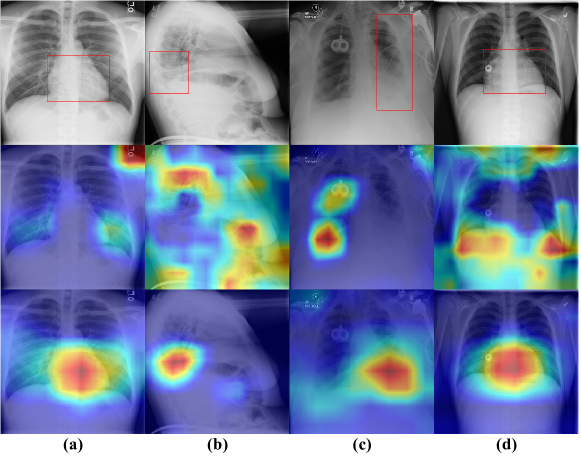
Figure 1: Some tough cases in the data set. Each column is the same CXR image, and each row from top to bottom shows the original image with a pathological bounding box, weighted heat maps of traditional CNN-based deep learning, and our proposed method, in that order. Four difficult situations such as (a): letters on images, (b): irregular images, (c): medical devices on images, and (d): easily confused between classes.

In order to effectively solve the above problems, we model the CXR image classification task from a causal perspective. We sort out the relationships among the causal feature, the confounding feature, and the classification result. In a nutshell, our basic idea is “borrow from others.” We also stick with letters in an image as an example. If part of the image is marked with letters, this situation affects the classification of the unmarked image, because we think of the letters as a confounding element, When we borrow the mark from the unmarked image, it is equivalent to eliminating the confounding effect. The same is true for other confounding assumptions we mentioned.

Towards this end, we utilize causal inference to minimize the confounding effect and maximize the causal effect while achieving stable and decent performance. Specifically, we first utilize traditional CNN-based modules to extract the feature from the input CXR images, and then apply Transformer decoder [19] based cross-attention mechanism to produce the estimations of the causal and latent confounding features from the feature maps. After that, we can parameterize the backdoor adjustment in the causal theory[14], which combines every causal estimation with different confounding estimations and encourages these combinations to remain a stable classification performance via the idea of “borrow from others”. It tends to facilitate the invariance between the causal patterns and the classification results.

We apply the method to different data sets and the experimental results demonstrate the performance and superiority of our approach. Our contributions can be summarized as follows:

• We take a casual look at the chest X-ray images’ multi-label classification problem and model the disordered or easily-confused part of an image as the confounder.

• We propose a framework based on the guideline of backdoor adjustment and presented a novel strategy for chest X-ray image classification. It allows a properly designed model to exploit real and stable causal features while removing the effects of filtrable confounding patterns.

• Extensive experiments on two large-scale public datasets justify the effectiveness of our proposed method. More visualizations with detailed analysis demonstrate the interpretability and rationalization of our proposed method.

2 Methodology

In this section, we first define the causal model, then identify the strategies to eliminate confounding effects.

2.1 A Causal View on CXR Images

From the above discussion, we construct a Structural Causal Model (SCM) [2]in Fig. 2(a) to solve the spurious correlation problems in CXR. It contains the causalities about four elements: Input CXR image data $D$, confounding feature $C$, causal feature $X$, and prediction $Y$, where the arrows between elements stand for cause and effect: cause $\rightarrow$ effect. We have the following explanations for the SCM in our task:

• $C\leftarrow D\rightarrow S$: $X$ denotes the causal feature which really contributes to the diagnosis, whereas $C$ denotes the confounding feature which may mislead the diagnosis and usually caused by data bias and other complex situations mentioned above. The two arrows can be seen as the feature extraction process. Apparently, $C$ and $X$ usually coexist in the medical image data $D$, these causal effects are built naturally.

• $C\rightarrow Y\leftarrow X$: We denote $Y$ as the classification result which should have been caused only by $X$ but inevitably disturbed by confounding features. The two arrows can be implemented by classifiers.

The goal of the classification model should capture the true causality between the causal feature $X$ and the diagnostic result $Y$, avoiding the influence of the confounding feature $C$. For example, we hope in some complex cases, the model will diagnose via real pathology features rather than letters or medical devices in the input CXR image. However, the conventional correlation $P(Y|X)$ fails to achieve that because of the backdoor path [13] $X\leftarrow D\rightarrow C\rightarrow Y$ between $X$ and $Y$. Therefore, we choose to apply the causal intervention to cut off the backdoor path and use $P(Y|do(X))$ to replace $P(Y|X)$, so the model has the ability to exploit causal features.

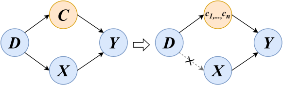
Figure 2: Structural causal model for CXR image classification. “D” is the input data, “C” denotes the confounding features, “X” is the causal features and “Y” is the prediction results.

2.2 Causal Intervention via Backdoor Adjustment

In this section, we propose to use the backdoor adjustment [2] to implement $P(Y|do(X))$ and eliminate the backdoor path, which is shown in Fig. 2(b). The backdoor adjustment assumes that we can observe and stratify the confounders, i.e., $C=\{c_{1},c_{2},...,c_{n}\}$, where each $c$ is a stratification of the confounder feature. We can then exploit the powerful do-calculus on causal feature $X$ by estimating $P_{b}(Y|X)=P(Y|do(X))$, where the subscript $b$ denotes the backdoor adjustment on the SCM.

Causal theory [14] provides us with three key conclusions:

• $P(c)=P_{b}(c)$: the marginal probability is invariant under the intervention, because $C$ will remain unchanged when cutting the link between $D$ and $X$ as shown in Fig. 2(b).

• $P_{b}(Y|X,c)=P(Y|X,c)$: $Y$’s response to $X$ and $C$ has no connection with the causal effect between $X$ and $C$.

• $P_{b}(c|X)=P_{b}(c)$: $X$ and $C$ are independent after backdoor adjustment.

Based on the conclusions, the backdoor adjustment for the SCM in Fig. 2(a) is:

$$P(Y|do(X)) =P_{b}(Y|X)=\sum_{c\in\mathcal{C}}P_{b}(Y|X,c)P_{b}(c|X)$$ (1)

$$=\sum_{c\in\mathcal{C}}P_{b}(Y|X,c)P_{b}(c)=\sum_{c\in\mathcal{C}}P(Y|X,c)P(c),$$

where $\mathcal{C}$ denotes the confounder set, $P(c)$ is the prior probability of $c$. Then, we approximate the formula by a random sample operation which will be detailed next.

2.3 Training Object

Till now, we need to provide the implementations of Eq.(1) in a parameterized method to fit the deep learning model. However, in the medical scenario, $\mathcal{C}$ is complicated and hard to obtain, so we simplify the problem and assume a uniform distribution of confounders. Traditionally, when we want to drive the deep model to learn useful knowledge, we are always extremely dependent on the properly designed loss function. Then, towards effective backdoor adjustment, we utilize different loss functions to drive our deep model to learn causal and spurious features respectively. Fig. 3 illustrates the proposed network. Note that the channel and position attention is implemented by adopting an efficient variant of self-attention [12]. We will break the whole framework down in detail below.

Given an image $x\in\mathbb{R}^{H_{0}\times W_{0}\times 3}$ as input, we extract its spatial feature $F\in\mathbb{R}^{H\times W\times d}$ using the backbone, where $H_{0}\times W_{0}$, $H\times W$ represent the height and width of the CXR image and the feature map respectively, and $d$ denotes the hidden dimension of the network. Then, we adopt zero-initialized $Q_{0}\in\mathbb{R}^{C\times d}$ as the queries in the cross-attention module inside the transformer, each decoder layer $l$ updates the queries $Q_{l-1}$ from its previous layer. Here, we denote $Q$ as the causal feature and $\overline{Q}$ as the confounding feature as follows:

$$Q_{l}=softmax(\widetilde{Q}_{l-1}\widetilde{F}/\sqrt{dim_{\widetilde{F}}})F,$$ (2)

$$\overline{Q}_{l}=(1-softmax(\widetilde{Q}_{l-1}\widetilde{F}/\sqrt{dim_{F}}))F,$$

where the tilde in $\widetilde{F}$ means the feature with position encodings, the disentangled features yield two branches, which can be fed separately into a point-wise Multi-layer perceptron (MLP) network and get corresponding classification logits via a sigmoid function.

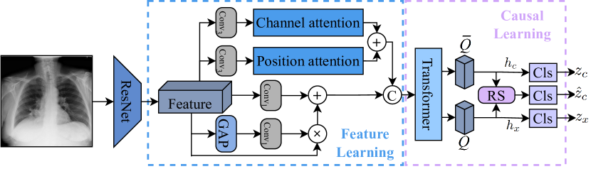
Figure 3: Overview of our network. Firstly, we apply CNN with modified attention to extract the image feature, where the $n$ in Conv_n denotes the kernel size of the convolutional operation, “+”, “$\times$”, and “C” denote add, multiply, and concatenate operations, respectively. “GAP” means global average pooling, “RS” is the random sample operation, and “Cls” denotes the classifier. The cross-attention module inside the transformer decoder disentangles the causal and confounding feature, then we can apply parameterized backdoor adjustment to achieve causal inference.

2.3.1 Disentanglement.

As shown in Fig. 3, we try to impel the model to learn both causal and confounding features via the designed model structure and loss function. Specifically, we adopt a CNN-based model to extract the feature of input images, then capture the causal feature and confounding feature by cross-attention mechanism. Thus we can make the prediction via MLP and classifiers:

$$h_{c}=MLP_{confounding}(\overline{Q_{l}}),z_{c}=\Phi_{c}(h_{c}),$$ (3)

$$h_{x}=MLP_{causal}(Q_{l}),z_{x}=\Phi_{x}(h_{x}),$$

where $h\in\mathbb{R}^{d\times C}$, $C$ is the number of categories, $\Phi(\cdot)$ represents classifier, $z$ denotes logits.

The causal part aims to estimate the really useful feature, so we apply the supervised classification loss in a cross-entropy format:

$$\mathcal{L}_{sl}=-\frac{1}{\lvert D\rvert}\sum_{d\in D}y^{\top}\log(z_{x}),$$ (4)

where $d$ is a sample and $D$ is the training data, $y$ is the corresponding label. The confounding part is unwanted for classification, so we follow the work in CAL [18] and push its prediction equally to all categories, then the confounding loss is defined as:

$$\mathcal{L}_{conf}=-\frac{1}{\lvert D\rvert}\sum_{d\in D}KL(y_{uniform},z_{c}),$$ (5)

where KL is the KL-Divergence, $y_{uniform}$ denotes a uniform distribution. We optimize the above two losses and can effectively disentangle causal and confounding features.

2.3.2 Causal intervention.

The idea of the backdoor adjustment formula in Eq.(1) is to stratify the confounder and combine confounding and causal features manually, which is also the implementation of the random sample in Fig. 3. For this propose, we stratify the extracted confounding feature and random add it to the other CXR images’ feature to be classified shown in Eq.(6), and get a “intervened graph”, then we have the following loss guided by causal inference:

$$\hat{z}_{c}=\Phi(h_{x}+\hat{h}_{c}),$$ (6)

$$\mathcal{L}_{bd}=-\frac{1}{\lvert D\rvert\cdot\lvert\hat{D}\rvert}\sum_{d\in D}\sum_{\hat{d}\in\hat{D}}y^{\top}\log(\hat{z}_{c}),$$ (7)

where $\hat{z}_{c}$ is the prediction from a classifier on the “intervened graph”, $\hat{h}_{c}$ is the stratification feature via Eq.(3), $\hat{D}$ is the estimated stratification set contains trivial features. The objective of our framework can be defined as the sum of the losses:

$$\mathcal{L}=\mathcal{L}_{sl}+\alpha_{1}\mathcal{L}_{conf}+\alpha_{2}\mathcal{L}_{bd},$$ (8)

where $\alpha_{1}$ and $\alpha_{2}$ are hyper-parameters, which decide how powerful disentanglement and backdoor adjustment are. It pushes the prediction stable because of the shared image features according to our detailed experimental results in the next section.

3 Experiments

3.1 Experimental Setup

We evaluate the common thoracic diseases classification performance on the NIH ChestX-ray14 [20] data set, which consists of 112,120 frontal-view CXR images with 14 diseases and we follow the official data split for a fair comparison.

In our experiments, we adopt ResNet101 [5] as the backbone. Our experiment is operated by using NVIDIA GeForce RTX 3090 with 24GB memory. We use the Adam [8] optimizer with a weight decay of 1$e$-2 and the max learning rate is 1$e$-3. On the NIH data set, we resize the original images to 512 $\times$ 512 as the input. We evaluate the classification performance of our method with the area under the ROC curve (AUC) for the whole test set.

3.2 Results and Analysis

Table. 1 illustrates the overall performance of the NIH Chest-Xray14 dataset of our proposed method compared with other previous state-of-art works, the best performance of each pathology is shown in bold. From the experiments on the NIH data set, we can conclude that we eliminate some spurious relationships inner and between CXR images from the classification results. Specifically, we can find that we are not only making progress in most categories but also dealing with some pathologies with high symbiotic dependence [20] such as cardiomegaly and infiltration. The visualization results in Fig. 1 prove that the issues raised were addressed.

Table 1: Comparation of AUC scores with previous SOTA works. We report the AUC with a 95% confidence interval (CI) of our method.

Abnormality	DNetLoc [4]	Xi et al. [11]	ImageGCN [10]	DGFN [3]	Ours
Atelectasis	0.77	0.77	0.80	0.82	0.81 (0.81, 0.82)
Cardiomegaly	0.88	0.87	0.89	0.93	0.94 (0.93, 0.95)
Effusion	0.83	0.83	0.87	0.88	0.91 (0.91, 0.92)
Infiltration	0.71	0.71	0.70	0.75	0.75 (0.74, 0.77)
Mass	0.82	0.83	0.84	0.88	0.89 (0.88, 0.90)
Nodule	0.76	0.79	0.77	0.79	0.76 (0.74, 0.79)
Pneumonia	0.73	0.82	0.72	0.78	0.82 (0.80, 0.83)
Pneumothorax	0.85	0.88	0.90	0.89	0.91 (0.91, 0.93)
Consolidation	0.75	0.74	0.80	0.81	0.82 (0.81, 0.83)
Edema	0.84	0.84	0.88	0.89	0.90 (0.89, 0.90)
Emphysema	0.90	0.94	0.92	0.94	0.94 (0.93, 0.95)
Fibrosis	0.82	0.83	0.83	0.82	0.84 (0.84, 0.85)
Pleural_Thicken	0.76	0.79	0.79	0.81	0.77 (0.75, 0.78)
Hernia	0.90	0.91	0.94	0.92	0.94 (0.92, 0.95)
Mean AUC	0.807	0.819	0.832	0.850	0.857 (0.849, 0.864)

Ablation studies on the NIH data set are shown in Table. 4. Where “+” denotes utilize the module whereas “-” denotes remove the module. We demonstrate the efficiency of our method from the ablation study, we can find that our feature extraction and causal learning module play significant roles, respectively. Besides, during the training process, Fig. 4 shows the fluctuation of the classification effect of three classifiers, where the three lines in the diagram correspond to the three classifiers in Fig. 3. We can find the performance of the confounding classifier goes up at first and then down. At the same time, the other two classifiers’ performance increased gradually, which is in line with our expectations. Our proposed causal learning framework successfully discards the adverse effect of confounding features and makes the prediction stable.

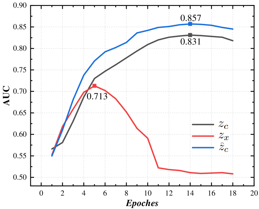
Figure 4: Fluctuation of classification effect of three classifiers.

Table 2: Ablation study on NIH data set.

Model	Feature Learning	Causal Learning	AUC
1	-	-	0.812
2	-	+	0.833
3	+	-	0.824
4	+	+	0.857

4 Conclusion

In conclusion, we present a novel causal inference-based chest X-ray image multi-label classification framework from a causal perspective, which comprising a feature learning module and a backdoor adjustment-based causal inference module. We find that previous deep learning based strategies are prone to make the final prediction via some spurious correlation, which plays a confounder role then damage the performance of the model. We evaluate our proposed method on the public data set, experimental results indicate that our proposed framework and method are superior to previous state-of-the-art methods.

References

- [1] Brady, A., Laoide, R.Ó., McCarthy, P., McDermott, R.: Discrepancy and error in radiology: concepts, causes and consequences. The Ulster medical journal 81(1), 3 (2012)
- [2] Glymour, M., Pearl, J., Jewell, N.P.: Causal inference in statistics: A primer. John Wiley & Sons (2016)
- [3] Gong, X., Xia, X., Zhu, W., Zhang, B., Doermann, D., Zhuo, L.: Deformable gabor feature networks for biomedical image classification. In: Proceedings of the IEEE/CVF Winter Conference on Applications of Computer Vision. pp. 4004–4012 (2021)
- [4] Guendel, S., Grbic, S., Georgescu, B., Liu, S., Maier, A., Comaniciu, D.: Learning to recognize abnormalities in chest x-rays with location-aware dense networks. In: Iberoamerican Congress on Pattern Recognition. pp. 757–765. Springer (2018)
- [5] He, K., Zhang, X., Ren, S., Sun, J.: Deep residual learning for image recognition. In: Proceedings of the IEEE conference on computer vision and pattern recognition. pp. 770–778 (2016)
- [6] Irvin, J., Rajpurkar, P., Ko, M., Yu, Y., Ciurea-Ilcus, S., Chute, C., Marklund, H., Haghgoo, B., Ball, R., Shpanskaya, K., et al.: Chexpert: A large chest radiograph dataset with uncertainty labels and expert comparison. In: Proceedings of the AAAI conference on artificial intelligence. vol. 33, pp. 590–597 (2019)
- [7] Ke, A., Ellsworth, W., Banerjee, O., Ng, A.Y., Rajpurkar, P.: Chextransfer: performance and parameter efficiency of imagenet models for chest x-ray interpretation. In: Proceedings of the Conference on Health, Inference, and Learning. pp. 116–124 (2021)
- [8] Kingma, D.P., Ba, J.: Adam: A method for stochastic optimization. arXiv preprint arXiv:1412.6980 (2014)
- [9] Liu, H., Wang, L., Nan, Y., Jin, F., Wang, Q., Pu, J.: Sdfn: Segmentation-based deep fusion network for thoracic disease classification in chest x-ray images. Computerized Medical Imaging and Graphics 75, 66–73 (2019)
- [10] Mao, C., Yao, L., Luo, Y.: Imagegcn: Multi-relational image graph convolutional networks for disease identification with chest x-rays. IEEE Transactions on Medical Imaging (2022)
- [11] Ouyang, X., Karanam, S., Wu, Z., Chen, T., Huo, J., Zhou, X.S., Wang, Q., Cheng, J.Z.: Learning hierarchical attention for weakly-supervised chest x-ray abnormality localization and diagnosis. IEEE Transactions on Medical Imaging (2020)
- [12] Pan, X., Ge, C., Lu, R., Song, S., Chen, G., Huang, Z., Huang, G.: On the integration of self-attention and convolution. In: Proceedings of the IEEE/CVF Conference on Computer Vision and Pattern Recognition. pp. 815–825 (2022)
- [13] Pearl, J.: Interpretation and identification of causal mediation. Psychological methods 19(4), 459 (2014)
- [14] Pearl, J., et al.: Models, reasoning and inference. Cambridge, UK: CambridgeUniversityPress 19(2) (2000)
- [15] Rajaraman, S., Antani, S.: Training deep learning algorithms with weakly labeled pneumonia chest x-ray data for covid-19 detection. MedRxiv (2020)
- [16] Rocha, J., Pereira, S.C., Pedrosa, J., Campilho, A., Mendonça, A.M.: Attention-driven spatial transformer network for abnormality detection in chest x-ray images. In: 2022 IEEE 35th International Symposium on Computer-Based Medical Systems (CBMS). pp. 252–257. IEEE (2022)
- [17] Saleem, H.N., Sheikh, U.U., Khalid, S.A.: Classification of chest diseases from x-ray images on the chexpert dataset. In: Innovations in Electrical and Electronic Engineering, pp. 837–850. Springer (2021)
- [18] Sui, Y., Wang, X., Wu, J., Lin, M., He, X., Chua, T.S.: Causal attention for interpretable and generalizable graph classification. In: Proceedings of the 28th ACM SIGKDD Conference on Knowledge Discovery and Data Mining. pp. 1696–1705 (2022)
- [19] Vaswani, A., Shazeer, N., Parmar, N., Uszkoreit, J., Jones, L., Gomez, A.N., Kaiser, Ł., Polosukhin, I.: Attention is all you need. Advances in neural information processing systems 30 (2017)
- [20] Wang, X., Peng, Y., Lu, L., Lu, Z., Bagheri, M., Summers, R.M.: Chestx-ray8: Hospital-scale chest x-ray database and benchmarks on weakly-supervised classification and localization of common thorax diseases. In: Proceedings of the IEEE conference on computer vision and pattern recognition. pp. 2097–2106 (2017)
- [21] Zhang, Y., Kang, B., Hooi, B., Yan, S., Feng, J.: Deep long-tailed learning: A survey. arXiv preprint arXiv:2110.04596 (2021)