YOLO: An Efficient Terahertz Band Integrated Sensing and Communications Scheme with
Beam Squint

Abstract

Using communications signals for dynamic target sensing is an important component of integrated sensing and communications (ISAC). In this paper, we propose to utilize the beam squint effect to realize fast non-cooperative dynamic target sensing in massive multiple input and multiple output (MIMO) Terahertz band communications systems. Specifically, we construct a wideband channel model of the echo signals, and design a beamforming strategy that controls the range of beam squint by adjusting the values of phase shifters and true time delay lines. With this design, beams at different subcarriers can be aligned along different directions in a planned way. Then the received echo signals at different subcarriers will carry target information in different directions, based on which the targets’ angles can be estimated through sophisticatedly designed algorithm. Moreover, we propose a supporting method based on extended array signal estimation, which utilizes the phase changes of different frequency subcarriers within different orthogonal frequency division multiplexing (OFDM) symbols to estimate the distances and velocities of dynamic targets. Interestingly, the proposed sensing scheme only needs to transmit and receive the signals once, which can be termed as You Only Listen Once (YOLO). Compared with the traditional ISAC methods that require time consuming beam sweeping, the proposed one greatly reduces the sensing overhead. Simulation results are provided to demonstrate the effectiveness of the proposed schemes.

I Introduction

Integrated sensing and communications (ISAC) is anticipated to be a key technology of sixth generation (6G) mobile communications [1, 2, 3]. Its basic idea is to use communication signals to sense various aspects of the real physical world, such as target’s position, architectural composition, human activity, etc. Once the ISAC system obtains such information, it can not only enhance the data transmission performance[4], but also support a variety of intelligent applications, such as connected vehicles and smart factory[5, 6].

As the decisive function of ISAC, the ultimate functionality of sensing is to construct a mapping relationship from the real physical world to the digital twin world. Note that the real physical world is composed of static environments (such as roads and buildings) and dynamic targets (such as pedestrians and vehicles). The changes of static environment are usually slow, and thus one can apply various environmental reconstruction technologies to sense the static environment[7, 8, 9]. However, since the changes of dynamic targets are rapid, it is necessary to update the parameters of dynamic targets in real-time. Generally, the dynamic targets sensing problem can be classified into two categories: (1) sensing cooperative communications users, e.g., mobile phones; and (2) sensing non-cooperative dynamic targets that are not communicating with the base station (BS), e.g., moving objects or users not in communications status.

In massive multiple input and multiple output (MIMO) arrays based ISAC systems, a series of signal processing algorithms can be implemented for sensing cooperative users. For example, by processing the pilot signals of the communications system, the time of arrival (TOA), and the angle of departure (AOD), etc., can be extracted to estimate a user’s position[10, 11, 12, 13]. The sensing of non-cooperative targets has traditionally been accomplished via radar systems[14, 15, 16]. Currently, there are many works focusing on non-cooperative target sensing under ISAC framework. For example, Z. Gao et. al. proposed an ISAC processing framework relying on MIMO systems, which applied compressed sampling to facilitate target sensing and other processing[17]. Z. Wang et. al. proposed a simultaneously transmitting and reflecting surface enabled ISAC framework, in which the two-dimensional maximum likelihood estimation was utilized to estimate the direction-of-arrival of the sensing target[18]. C. Mush et. al. studied the potential applications of autoencoders in ISAC systems and presented a novel perspective on target detection[19]. However, these works consider only the sensing of static targets, which entails difficulty in practical scenarios where static targets are coupled with static environments and are difficult to separate. In terms of non-cooperative dynamic target sensing, Y. Li et. al. proposed a two-stage algorithm using orthogonal frequency division multiplexing (OFDM) signals to estimate the parameters of targets[20]. P. Kumari et. al. proposed an ISAC system for the internet of vehicles, which realized vehicle to vehicle communications and full duplex radar sensing[21]. X. Chen et. al. proposed a multiple signal classification based ISAC system that can attain high estimation accuracy for dynamic target sensing[22]. Z. Wei et. al. proposed the use of the iterative two-dimensional fast Fourier transform and iterative cyclic cross-correlation methods to realize short distance and long distance dynamic target sensing, respectively[23]. Z. Han et. al. designed a novel multistatic MIMO-ISAC system in cellular networks, and made the use of widespread BSs to perform dynamic target sensing over a wide area[24]. Nevertheless, although these approaches consider the sensing of dynamic targets, they do not address the serious interference caused by static environmental clutter on dynamic target sensing, thus limiting the sensing performance in some practical scenarios.

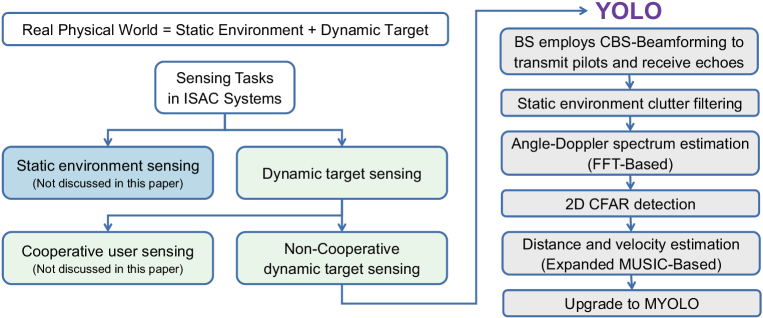
Figure 1: ISAC sensing task classification and flowchart of the proposed YOLO sensing scheme.

In addition, the aforementioned algorithms for dynamic target sensing consider only narrowband signals, while wideband signals from mmWave and Terahertz frequency bands are expected to dominate in 6G communications[25, 26]. Specially, Terahertz communications is recognized as a highly promising technology for the 6G and beyond era, due to its unique potential to support terabit-per-second transmission in emerging applications[27, 28]. Meanwhile, sensing in the Terahertz band with MIMO can achieve higher accuracy thanks to the corresponding high directivity and high temporal resolution[29, 30]. Nevertheless, it is by no means straightforward or may even be infeasible to extend narrowband sensing algorithms to wideband scenarios. For example, [31] and [32] showed that for a wideband Terahertz system, the beam squint phenomenon would appear, in which the beams from different subcarriers would disperse to different directions, making beam directions of some subcarriers deviate from the desired direction. Beam squint is usually considered to be a negative effect for communications and should be mitigated with the aid of true time delay lines[33, 34, 35]. Interestingly, some works have recently tried to enhance the sensing performance through reverse utilization of beam squint. For example, the authors of [36] proposed a user angle sensing scheme with low pilot overhead based on beam squint and beam split, but they did not consider distance and velocity estimation or more general non-cooperative dynamic target sensing tasks.

In this paper, we propose an efficient non-cooperative dynamic target sensing scheme for Terahertz ISAC systems with the aid of the beam squint effect, in which the BS can quickly sense the dynamic target’s position and velocity through frequency-domain estimation. The contributions of this paper are summarized as follows.

• We consider, for the first time, both the static environment and the dynamic targets in the ISAC scenario, and derive a corresponding wideband echo channel model in the time-frequency domain.

• We analyze the beam squint effect in wideband ISAC systems and propose a controllable beam squint strategy to assist sensing, which is termed CBS-Beamforming.

• We utilize the controllable beam squint to realize fast sensing of non-cooperative dynamic targets, in which the BS only needs to transmit and receive the OFDM signal once to obtain the positions and velocities of all targets in the entire area. This scheme is termed you only listen once (YOLO), and a flowchart of it is presented in Fig. 1.

• We improve the accuracy of sensing by performing YOLO multiple times with different beam squint ranges, which technique is termed Multiple YOLO (MYOLO).

• We provide various simulations to demonstrate the effectiveness of the proposed schemes.

The remainder of this paper is organized as follows. In Section II, we introduce the wideband channel model involving both the static environment and the dynamic targets. In Section III, the beam squint effect is analyzed and the beamforming strategy based on controllable beam squint is derived. Then we propose the dynamic target sensing algorithms in Section IV. Simulation results and conclusions are given in Section V and Section VI, respectively.

Notation: Lower-case and upper-case boldface letters $\mathbf{a}$ and $\mathbf{A}$ denote vectors and matrices; $\mathbf{a}^{T}$ and $\mathbf{a}^{H}$ denote the transpose and the conjugate transpose of $\mathbf{a}$; ${\rm diag}(\mathbf{a})$ denotes a diagonal matrix with the diagonal elements constructed from $\mathbf{a}$; $[\mathbf{a}]_{n}$ denotes the $n$-th element of $\mathbf{a}$; $[\mathbf{A}]_{i,j}$ denotes the $(i,j)$-th element of $\mathbf{A}$; $\mathbf{A}[i_{1}:i_{2},:]$ is the submatrix composed of all elements in rows $i_{1}$ to $i_{2}$ of matrix $\mathbf{A}$; $\mathbf{A}[:,j_{1}:j_{2}]$ is the submatrix composed of all elements in columns $j_{1}$ to $j_{2}$ of matrix $\mathbf{A}$; Symbol 1 represents the all-ones matrix or vector with compatible dimensions; $\left|\cdot\right|$ denotes the absolute operator; and ${\rm eig}(\cdot)$ represents the eigenvalue decomposition function.

II System Model

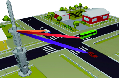
(a)

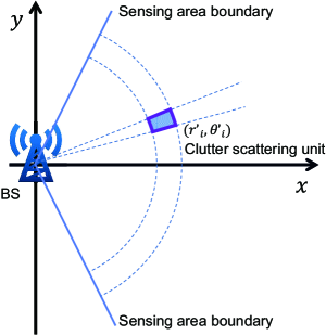
(b)

Figure 2: (a) System model. (b) Schematic diagram of clutter scattering unit.

Let us consider a massive MIMO system operating in the Terahertz frequency band with OFDM modulation. The BS is equipped with a uniform linear array (ULA) of $N$ antennas, where the antenna spacing is $d\leq\frac{\lambda}{2}$ and $\lambda$ is the wavelength. All antennas are located on the y-axis, and the position of the $n$-th antenna is $(0,nd)$, where $n=-\frac{N-1}{2},...,\frac{N-1}{2}$. Assume that the BS employs a single radio frequency (RF) chain for sensing. The carrier frequency and the transmission bandwidth are $f_{c}$ and $W$, respectively, and thus the passband frequency range is $[f_{c}-\frac{W}{2},f_{c}+\frac{W}{2}]$. Suppose there are $M+1$ subcarriers in total, where the $0$-th subcarrier has the lowest frequency $f_{0}=f_{c}-\frac{W}{2}$, and the $m$-th subcarrier frequency is $f_{m}=f_{0}+m\frac{W}{M}$. Let us denote the baseband frequency of the $m$-th subcarrier as $\widetilde{f}_{m}=m\frac{W}{M}$, where $m=0,1,2,...,M$. Obviously, there is $f_{m}=f_{0}+\widetilde{f}_{m}$. Assume that the BS works in full duplex mode and has perfect self-interference cancellation. We suppose that the BS enables an OFDM block containing $N_{s}$ consecutive OFDM symbols to realize dynamic target sensing, and the symbol duration is $T_{s}=\frac{1}{\Delta f}=\frac{1}{W/M}$, where $\Delta f=\frac{W}{M}$ is the subcarrier frequency spacing.

As shown in Fig. 2(a), the real physical world scene is typically composed of static environment and dynamic targets. When the BS sends the probing signal to the coverage area at the beginning of sensing, the receiving array will receive effective echoes caused by dynamic targets of interest (dynamic target echo) and undesired dense echoes caused by uninteresting background environments. In radar systems, the undesired dense echoes are usually referred to as “clutter”, including ground clutter, sea clutter, weather clutter, etc[37]. The key difference between dynamic target echoes and clutter lies in their different Doppler frequencies. That is, the Doppler frequency of a dynamic target echo is usually much higher than that of clutter, while the Doppler frequency of clutter is usually zero or a small non-zero value. Specifically, as the main component of urban environmental clutter, ground clutter is usually caused by static objects, such as land, mountains, roads, buildings, etc, and its signal power intensity is usually about $50$ dB higher than that of the dynamic target echo, but its Doppler frequency is almost zero. Based on the above analysis, a practical modeling of echo signals should include both dynamic target echoes and static environment echoes, and the BS needs to perform a series of signal processing to accurately detect and estimate the dynamic targets in a strong clutter background. However, some existing ISAC works[17, 18, 19] have not considered the objective existence of static environmental clutter and have instead directly assumed that the stationary targets could be observed. Although some other ISAC works[20, 21, 22, 23, 24] have focused on dynamic target sensing, they have not considered the serious interference caused by static environmental clutter.

Here we model the clutter of ISAC system based on a typical urban service scenario, in which the static environment can be divided into a finite number of grid units. That is, we divide the effective clutter area within the sensing range into equal intervals based on distance and angle dimensions, ultimately achieving a division of the static environment into a limited number of scattering units as illustrated by the blue grid in Fig. 2(b). The size of each clutter scattering unit is determined by the angle resolution and distance resolution of the system. Assume that the sensing range is divided into $I$ static clutter scattering units, where the position of the $i$-th static clutter scattering unit is denoted as $(r_{i}^{\prime},\theta_{i}^{\prime})$. Then the echo channel of this unit on the $m$-th subcarrier of the $n_{s}$-th OFDM symbol can be modeled as

$$\begin{split}\begin{aligned} \mathbf{H}_{i,n_{s},m}^{\prime}=\beta_{i}e^{-j2\pi f_{m}\frac{2r_{i}^{\prime}}{c}}\mathbf{a}_{m}(\theta_{i}^{\prime})\mathbf{a}_{m}^{T}(\theta_{i}^{\prime})\in\mathbb{C}^{N\times N},\end{aligned}\end{split}$$ (1)

where $\mathbf{a}_{m}(\theta)\in\mathbb{C}^{N\times 1}$ represents the steering vector of the antenna array towards the angle $\theta$ on the $m$-th subcarrier, the $n$-th element in $\mathbf{a}_{m}(\theta)$ is $[\mathbf{a}_{m}(\theta)]_{n}=e^{j\frac{2\pi f_{m}}{c}nd\sin\theta}$, $\beta_{i}=\sqrt{\frac{\lambda^{2}}{(4\pi)^{3}(r^{\prime}_{i})^{4}}}\sigma_{c,i}^{\prime}$, and $\sigma_{c,i}^{\prime}$ is the radar cross section (RCS) of the $i$-th static clutter scattering unit. The RCS of ground clutter can be modeled using the Swerling $\rm I$ model[38], in which the probability density function (PDF) of the RCS $\sigma$ satisfies

$$\begin{split}\begin{aligned} f(\sigma)=\frac{1}{\sigma_{0}}\exp(-\frac{\sigma}{\sigma_{0}}),\sigma\geq 0,\end{aligned}\end{split}$$ (2)

where $\sigma_{0}$ is the mean value of the RCS.

In addition, we assume that there are $K$ dynamic targets within the sensing range of the BS. The two-dimensional position of the $k$-th dynamic target is $(x_{k},y_{k})$, the corresponding polar coordinate is $(r_{k},\theta_{k})$, and the radial velocity of the $k$-th dynamic target is $v_{k}$. Then the distance between the $k$-th dynamic target and the $n$-th antenna of the BS is

$$\begin{split}\begin{aligned} r_{k,n}&=\sqrt{x_{k}^{2}\!+\!(y_{k}\!-\!nd)^{2}}\approx r_{k}-nd\sin\theta_{k}.\end{aligned}\end{split}$$ (3)

Then the echo channel corresponding to the $k$-th dynamic target on the $m$-th subcarrier of the $n_{s}$-th OFDM symbol is

$$\begin{split}\begin{aligned} \mathbf{H}_{k,n_{s},m}=\alpha_{k}e^{j2\pi f_{0}\frac{2v_{k}}{c}n_{s}T_{s}}e^{-j2\pi f_{m}\frac{2r_{k}}{c}}\mathbf{a}_{k,m}\mathbf{a}_{k,m}^{T},\end{aligned}\end{split}$$ (4)

where $\mathbf{a}_{k,m}\in\mathbb{C}^{N\times 1}$ represents the steering vector of the BS antennas with the $n$-th element $[\mathbf{a}_{k,m}]_{n}=e^{j\frac{2\pi f_{m}}{c}nd\sin\theta_{k}}$, $\alpha_{k}$ is modeled as $\alpha_{k}=\sqrt{\frac{\lambda^{2}}{(4\pi)^{3}r_{k}^{4}}}\sigma_{c,k}$, and $\sigma_{c,k}$ is the RCS of the $k$-th dynamic target, also following the Swerling $\rm I$ model.

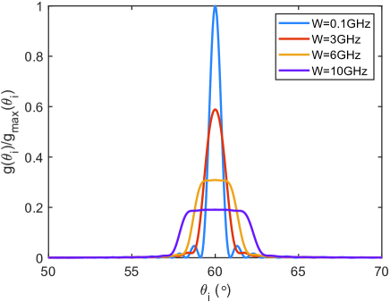
(a)

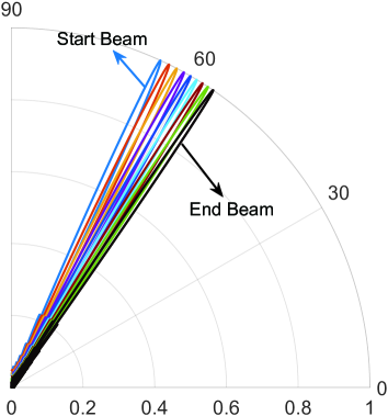
(b)

Figure 3: (a) An example of time-division beam sweeping, where the single target is located at $60^{\circ}$ and $f_{0}=220$ GHz. (b) Antenna array radiation pattern of BS under beam squint, where $f_{0}=220$ GHz, $W=22$ GHz and the central frequency subcarrier is focused at $60^{\circ}$.

Based on (1) and (4), the overall ISAC echo channel on the $m$-th subcarrier of the $n_{s}$-th symbol can be represented as

$$\begin{split}\begin{aligned} \mathbf{H}_{n_{s},m}=\sum_{k=1}^{K}\!\mathbf{H}_{k,n_{s},m}+\sum_{i=1}^{I}\!\mathbf{H}_{i,n_{s},m}^{\prime}.\end{aligned}\end{split}$$ (5)

Eq. (5) indicates that the echo channel of the ISAC system should be the sum of the background environment channel and the dynamic targets channel.

III Sensing Oriented Beamforming with Controllable Beam Squint

Massive MIMO systems are usually combined with beamforming technology to compensate for the high propagation loss of mmWave or Terahertz signals and enhance the directional communications and sensing performance[39, 40]. However, directly applying beamforming for sensing requires a long beam sweeping time as it did in existing ISAC or the conventional radar systems[41, 42]. Meanwhile, it has been shown in [31] and [43] that for a Terahertz communications system, the beam squint effect would appear, in which the beams from different subcarriers would point to different directions, making the signals on some subcarriers deviate from the desired direction.

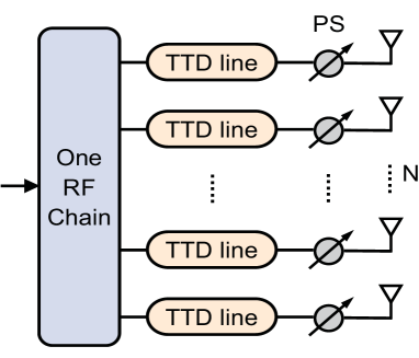
(a)

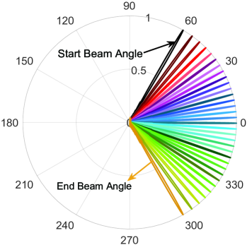
(b)

Figure 4: (a) TTDs-assisted BS antenna array links. (b) An example of controllable beam squint.

III-A The Influence of Beam Squint on Sensing

Suppose the beamforming vectors used during transmitting and receiving signals are $\mathbf{w}_{t}$ and $\mathbf{w}_{r}$, respectively. Assume that the frequency-domain probing data sent by the BS is $\mathbf{s}=\mathbf{1}\in\mathbb{C}^{(M+1)\times 1}$ and consider the noiseless case. Then the received echo signal on the $m$-th subcarrier of the $n_{s}$-th symbol is

$$\begin{split}\begin{aligned} y_{n_{s},m}=\mathbf{w}_{r}^{H}\mathbf{H}_{n_{s},m}(\mathbf{w}_{t}^{H})^{T}.\end{aligned}\end{split}$$ (6)

Since the receiving and transmitting antennas are at the same location, the directions of departure and arrival associated with the target are the same. Hence $\mathbf{w}_{r}$ is generally the same as $\mathbf{w}_{t}$. In the traditional sensing, the BS searches the entire angle space via time domain beam sweeping. Suppose the BS uses $L$ beam sweeps, where the $l$-th beam sweep points to angle $\theta_{l}$. Then the beamforming vector used for the $l$-th beam sweep is

$$\begin{split}\begin{aligned} &\mathbf{w}_{t,l}=\mathbf{w}_{r,l}=\frac{1}{\sqrt{N}}\mathbf{a}(\theta_{l})\\ &=\frac{1}{\sqrt{N}}[e^{j\frac{2\pi f_{c}}{c}(-\frac{N-1}{2})d\sin\theta_{l}},...,e^{j\frac{2\pi f_{c}}{c}(\frac{N-1}{2})d\sin\theta_{l}}]^{T}.\end{aligned}\end{split}$$ (7)

Thus the total power of echo signals from all subcarriers in the $l$-th beam sweep is

$$\begin{split}\begin{aligned} g(\theta_{l})&=\sum_{m=0}^{M}|y_{n_{s},m,l}|=\sum_{m=0}^{M}|\mathbf{w}_{r,l}^{H}\mathbf{H}_{n_{s},m}(\mathbf{w}_{t,l}^{H})^{T}|\\ &=\sum_{m=0}^{M}\left|\frac{1}{N}\mathbf{a}^{H}(\theta_{l})\mathbf{H}_{n_{s},m}(\mathbf{a}^{H}(\theta_{l}))^{T}\right|.\end{aligned}\end{split}$$ (8)

Assume that the static clutter filtering has been performed on $y_{n_{s},m,l}$. Then the targets’ angles can be estimated by finding the peak values of $g(\theta_{l})$ after $L$ beam sweeps.

Fig. 3(a) shows an example of the curve $g(\theta_{l})$ when a single target is fixed at $60^{\circ}$ and $f_{0}=220$ GHz. If the transmission bandwidth $W$ is small (i.e., the narrowband signal), then the angle of the target can be well distinguished from the peak of $g(\theta_{l})$. However, if $W$ is large (i.e., the wideband signal), then the peak in $g(\theta_{l})$ gradually disappears, which deteriorates the resolution of angle estimation. To explain this phenomenon, we plot the antenna array radiation patterns on different subcarriers in Fig. 3(b). It is seen that when the central frequency subcarrier points to $60^{\circ}$ with $\mathbf{w}=\frac{1}{\sqrt{N}}\mathbf{a}(60^{\circ})$, the beamforming directions of other subcarriers gradually squint to other angles. Clearly, the beam squint effect leads to energy leakage for sensing, which then causes the flattening of the peak in Fig. 3(a).

III-B Utilizing Beam Squint for Sensing

To deal with this harmful beam divergence problem, the traditional solutions adopt the true time delay lines (TTDs) to re-concentrate all subcarriers into one direction[43]. Nevertheless, we can actually take advantage of the beam squint effect to cover a wide area within one single OFDM symbol. As shown in Fig. 4(a), we assume that each antenna is configured with a phase shifter (PS) and a TTD. Denote the $n$-th phase shifter response as $e^{-j2\pi\phi_{n}}$. The time domain response of the $n$-th TTD is $\delta(t-t_{n})$, and its frequency domain response is $e^{-j2\pi\widetilde{f}t_{n}}$. Then, the array beamforming vector assisted by TTDs can be expressed as

$$\begin{split}\begin{aligned} [\widetilde{\mathbf{w}}]_{n}=\frac{1}{\sqrt{N}}e^{-j2\pi\phi_{n}}e^{-j2\pi\widetilde{f}t_{n}},\end{aligned}\end{split}$$ (9)

where $\phi_{n}$ denotes the phase shift of the $n$-th PS, $t_{n}$ denotes the time delay of the $n$-th TTD, and $\widetilde{f}$ is the baseband frequency.

The steering vector of any angle direction $\theta$ on the $m$-th subcarrier is $\mathbf{a}_{m}(\theta)\in\mathbb{C}^{N\times 1}$, where $[\mathbf{a}_{m}(\theta)]_{n}=e^{j\frac{2\pi f_{m}}{c}nd\sin\theta}.$ With TTDs, the array gain on the $m$-th subcarrier is

$$\begin{split}\begin{aligned} g_{m}&=\left|\widetilde{\mathbf{w}}^{H}\cdot\mathbf{a}_{m}(\theta)\right|\\ &=\frac{1}{\sqrt{N}}\left|\sum_{n=-\frac{N-1}{2}}^{\frac{N-1}{2}}e^{j2\pi\phi_{n}}e^{j2\pi\widetilde{f}_{m}t_{n}}e^{j\frac{2\pi f_{m}}{c}nd\sin\theta}\right|.\end{aligned}\end{split}$$ (10)

It is seen from (10) that $g_{m}$ reaches its maximum value when

$$\begin{split}\begin{aligned} \phi_{n}+\widetilde{f}_{m}t_{n}+f_{m}\frac{nd\sin\theta}{c}=0.\end{aligned}\end{split}$$ (11)

By adjusting the values of PSs, we can let the beamforming at the $0$-th subcarrier $f_{0}$ point to a start angle $\theta_{start}$. Specifically, we set ${f}_{m}={f}_{0}$, $\widetilde{f}_{m}=\widetilde{f}_{0}=0$, $\theta=\theta_{start}$ in (11), and derive $\phi_{n}=-\frac{f_{0}nd\sin{\theta_{start}}}{c}$. Then we set the phase shift of the $n$-th PS as $\phi_{n}$. On the other side, by adjusting the values of TTDs, we can let the beamforming at the $M$-th subcarrier $f_{M}$ point to an end angle $\theta_{end}$. Specifically, we set ${f}_{m}={f}_{M}$, $\widetilde{f}_{m}=\widetilde{f}_{M}=W$, $\theta=\theta_{end}$ in (11), and derive $t_{n}=-\frac{\phi_{n}}{W}-\frac{(f_{0}+W)nd\sin{\theta_{end}}}{Wc}$. Then we set the time delay of the $n$-th TTD line as $t_{n}$. Afterwards, the beams from the $0$-th subcarrier to the $M$-th subcarrier gradually squint from the start angle $\theta_{start}$ to the end angle $\theta_{end}$ in a controlled way. For subcarrier $f_{m}$, its beamforming angle $\theta_{m}$ still satisfies (11) and can be computed as follows. We substitute $\theta=\theta_{m}$, $\phi_{n}=-\frac{f_{0}nd\sin{\theta_{start}}}{c}$, $t_{n}=-\frac{\phi_{n}}{W}-\frac{(f_{0}+W)nd\sin{\theta_{end}}}{Wc}$ into (11), and then the beam squint angle ${\theta}_{m}$ should satisfy

$$\begin{split}\begin{aligned} \sin{\theta}_{m}\!=\!\frac{(W\!-\!\widetilde{f}_{m})f_{0}}{Wf_{m}}\sin\theta_{start}\!+\!\frac{(W\!+\!f_{0})\widetilde{f}_{m}}{Wf_{m}}\sin\theta_{end}.\end{aligned}\end{split}$$ (12)

An example of controllable beam squint is shown in Fig 4(b), where $M=32$. By adjusting PSs and TTDs, we successfully control the start angle of beam squint as $\theta_{start}=60^{\circ}$ and the end angle as $\theta_{end}=-60^{\circ}$. Then all subcarriers gradually squint from $60^{\circ}$ to $-60^{\circ}$, which covers the entire space. When $M$ is large enough, all subcarriers can cover the whole sensing area within one single OFDM symbol. When $M=2048$, the average interval between adjacent subcarriers, i.e., the resolution is $\frac{120^{\circ}}{2048}=0.059^{\circ}$. We term the above beamforming scheme Beamforming Strategy with Controllable Beam Squint, i.e., CBS-Beamforming for short.

IV Dynamic Target Sensing Scheme Based on CBS-Beamforming

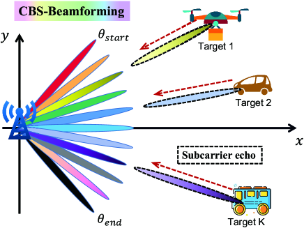
Figure 5: Dynamic target sensing system diagram based on CBS-Beamforming.

IV-A You Only Listen Once (YOLO): A Fast Sensing Scheme Based on CBS-Beamforming

Assume that the sensing range required by the BS is $[\theta_{start},\theta_{end}]$, and there are $K$ dynamic targets within the sensing range as shown in Fig. 5. Without loss of generality, we denote their positions as $(r_{1},\theta_{1}),(r_{2},\theta_{2}),...,(r_{K},\theta_{K})$, where $\theta_{start}>\theta_{1}>\theta_{2}>...>\theta_{K}>\theta_{end}$. According to (5), the echo channel matrix on the $m$-th subcarrier of the $n_{s}$-th symbol is $\mathbf{H}_{n_{s},m}$.

As illustrated in Fig. 5, the BS only needs one-time beam sweeping based on CBS-Beamforming to cover the whole sensing range, thanks to the dispersive effect of beam squint. With all $\mathbf{1}$ probing pilot, the received echo signal on the $m$-th subcarrier of the $n_{s}$-th symbol at the BS is

$$\begin{split}\begin{aligned} y_{n_{s},m}&=\widetilde{\mathbf{w}}^{H}\mathbf{H}_{n_{s},m}(\widetilde{\mathbf{w}}^{H})^{T}\\ &=\sum_{k=1}^{K}\alpha_{k}e^{j\frac{4\pi f_{0}v_{k}}{c}n_{s}T_{s}}e^{-j\frac{4\pi f_{m}r_{k}}{c}}\widetilde{\mathbf{w}}^{H}\mathbf{a}_{k,m}\mathbf{a}_{k,m}^{T}\widetilde{\mathbf{w}}^{*}\\ &\quad+\sum_{i=1}^{I}\beta_{i}e^{-j\frac{4\pi f_{m}r^{\prime}_{i}}{c}}\widetilde{\mathbf{w}}^{H}\mathbf{a}_{m}(\theta^{\prime}_{i})\mathbf{a}^{T}_{m}(\theta^{\prime}_{i})\widetilde{\mathbf{w}}^{*}.\end{aligned}\end{split}$$ (13)

Then the echo signals on all subcarriers and OFDM symbols can be combined into an echo signal matrix $\mathbf{Y}\in\mathbb{C}^{N_{s}\times(M+1)}$, and the $(n_{s},m)$-th element in $\mathbf{Y}$ is $[\mathbf{Y}]_{n_{s},m}=y_{n_{s},m}$, where $n_{s}=0,1,...,N_{s}-1$ and $m=0,1,2,...,M$.

For echo signal processing, some existing ISAC studies[17, 18, 19] only considered the sensing of static targets, and overlooked the widespread static environment. In fact, it is not easy to distinguish static targets from the static environment. Another part of ISAC studies [20, 21, 22, 23, 24] only considered the sensing of dynamic targets, and did not consider the serious interference caused by static environmental clutter on dynamic target sensing. In practice, it is difficult to directly detect and estimate dynamic targets in clutter backgrounds. Therefore, we must first filter out the dense echoes caused by static environments.

Considering that each scattering unit of the static environment does not cause significant Doppler frequency shift within $N$ consecutive OFDM symbols, we average each column of the echo signal matrix $\mathbf{Y}$ and obtain the echo signal vector caused by the static environment as $\mathbf{y}_{static}\in\mathbb{C}^{1\times(M+1)}$, whose $m$-th element is $[\mathbf{y}_{static}]_{m}=\frac{1}{N_{s}}\sum_{n_{s}=0}^{N_{s}-1}y_{n_{s},m}$. Note that $\mathbf{y}_{static}$ can be used to reconstruct the echo signal matrix caused by the static environment as $\mathbf{Y}_{static}=[\mathbf{y}^{T}_{static},...,\mathbf{y}^{T}_{static}]^{T}\in\mathbb{C}^{N_{s}\times(M+1)}$. Then the echo signal matrix caused by the dynamic targets can be extracted as $\mathbf{Y}_{dynamic}\!=\!\mathbf{Y}\!-\!\mathbf{Y}_{static}$, and we represent the $(n_{s},m)$-th element in $\mathbf{Y}_{dynamic}$ as

$$\begin{split}\begin{aligned} &\!\!\widetilde{y}_{n_{s},m}=\sum_{k=1}^{K}\alpha_{k}e^{j\phi{(\!k,\!n_{s},\!f_{m})}}\widetilde{\mathbf{w}}^{H}\mathbf{a}_{k,m}\mathbf{a}_{k,m}^{T}\widetilde{\mathbf{w}}^{*}-\mathcal{I}^{\prime}_{n_{s},m}\\ &\!\!\!\!\!\!=\!\!\sum_{k=1}^{K}\!\!\left\{\frac{\!\!\alpha_{k}e^{j\phi{(\!k\!,\!n_{s}\!,\!f_{m})}}}{N}\!\!\left[\!\sum_{n=-\frac{N-1}{2}}^{\frac{N-1}{2}}\!\!\!\!\!\!\!e^{\!j2\pi\phi_{n}}\!\!e^{j2\pi\widetilde{f}_{m}t_{n}}\!\!e^{\!j\!\frac{2\pi\!f_{m}}{c}\!n\!d\!\sin\!\theta_{k}}\!\!\right]^{2}\!\!\right\}\!-\!\!\mathcal{I}^{\prime}_{n_{s},m},\end{aligned}\end{split}$$ (14)

where $e^{j\phi{(k,n_{s},f_{m})}}=e^{j\frac{4\pi f_{0}v_{k}}{c}n_{s}T_{s}}e^{-j\frac{4\pi f_{m}r_{k}}{c}}$, $\mathcal{I}^{\prime}_{n_{s},m}$ is the remaining term introduced by clutter filtering. It is easy to prove that $\lim\limits_{N_{s}\to\infty}\mathcal{I}^{\prime}_{n_{s},m}=0$. In practical applications of radar systems, the term $\mathcal{I}^{\prime}_{n_{s},m}$ is usually ignored. Then we bring $\phi_{n}=-\frac{f_{0}nd\sin\theta_{start}}{c}$ and $t_{n}=-\frac{\phi_{n}}{W}-\frac{(f_{0}+W)nd\sin\theta_{end}}{Wc}$ into (14) and obtain

$$\begin{split}\begin{aligned} \widetilde{y}_{n_{s},m}\approx\!\!\frac{1}{N}\sum_{k=1}^{K}\left\{\alpha_{k}e^{j\phi{(k,n_{s},f_{m})}}\!\!\!\left[\frac{\sin(\frac{\beta(f_{m},\theta_{k})}{2}N)}{\sin(\frac{\beta(f_{m},\theta_{k})}{2})}\right]^{2}\right\},\end{aligned}\end{split}$$ (15)

where

$$\begin{split}\begin{aligned} &\!\!\!\!\beta(f_{m},\theta_{k})=\frac{2\pi d}{Wc}\times\\ &\!\!\!\![(W\!\!-\!\!\widetilde{f}_{m})\!f_{0}\!\sin\!\theta_{start}\!+\!(W\!\!+\!\!f_{0})\!\widetilde{f}_{m}\sin\!\theta_{end}\!-\!W\!f_{m}\sin\theta_{k}].\end{aligned}\end{split}$$ (16)

The detailed derivation of (15) can be found in Appendix A.

By taking the modulus of $\widetilde{y}_{n_{s},m}$, we can obtain the corresponding signal power as $g_{n_{s},m}=\left|\widetilde{y}_{n_{s},m}\right|$. Then the echo signal powers of all subcarriers and symbols can be pieced into a matrix $\mathbf{G}\in\mathbb{C}^{N_{s}\times(M+1)}$, which is called the power spectrum matrix of the echoes and satisfies $[\mathbf{G}]_{n_{s},m}=g_{n_{s},m}$. In addition, for the $n_{s}$-th OFDM symbol, the signal power of all subcarriers received during this symbol time can be pieced into a power spectrum vector $\mathbf{g}_{n_{s}}=[g_{n_{s},0},g_{n_{s},1},...,g_{n_{s},M}]^{T}\in\mathbb{C}^{(M+1)\times 1}$. Thus we have

$$\begin{split}\begin{aligned} \mathbf{G}=[\mathbf{g}_{0},\mathbf{g}_{1},...,\mathbf{g}_{N_{s}-1}]^{T}.\end{aligned}\end{split}$$ (17)

When $n_{s}$ is fixed, i.e., within the same OFDM symbol, it can be seen from (15) and (16) that $g_{n_{s},m}$ changes with the frequency $f_{m}$, and the powers of different subcarriers are different. In order to analyze the impacts from different targets, we designate a specific target as the $k^{*}$-th target, whose parameters are denoted as $r_{k^{*}}$, $\theta_{k^{*}}$ and $v_{k^{*}}$. For given $\theta_{k^{*}}$ in (16), $\beta(f_{m},\theta_{k^{*}})$ is a linear function of $f_{m}$, where $f_{m}=f_{0}+\widetilde{f}_{m}$ and $f_{0}\leq f_{m}\leq f_{M}=f_{0}+W$. Since $\theta_{k^{*}}$ belongs to $[\theta_{start},\theta_{end}]$, the product of the linear function’s terminal values is $\beta(f_{0},\theta_{k^{*}})\cdot\beta(f_{M},\theta_{k^{*}})=\frac{2\pi df_{0}}{c}(\sin\theta_{start}-\sin\theta_{k^{*}})\cdot\frac{2\pi df_{M}}{c}(\sin\theta_{end}-\sin\theta_{k^{*}})<0$. Hence there must exist an appropriate $f_{m}$ that makes $\beta(f_{m},\theta_{k^{*}})=0$ when the number of subcarriers $M+1$ is sufficiently large. Denote this frequency as $f^{d,k^{*}}_{m}$ and thus the constraint between $f^{d,k^{*}}_{m}$ and $\theta_{k^{*}}$ is $\beta(f^{d,k^{*}}_{m},\theta_{k^{*}})=0$. Let us then consider $2\ddot{M}+1$ subcarriers around the subcarrier $f^{d,k^{*}}_{m}$, whose frequencies can be denoted as $f^{d,k^{*}}_{m,-\ddot{M}},...,f^{d,k^{*}}_{m,0},...,f^{d,k^{*}}_{m,\ddot{M}}$ with $f^{d,k^{*}}_{m,\ddot{m}}=f^{d,k^{*}}_{m}+\ddot{m}\frac{W}{M}$, $\ddot{m}=-\ddot{M},...,\ddot{M}$ and $2\ddot{M}+1\ll M+1$. We record the beam squint angle corresponding to the subcarrier $f^{d,k^{*}}_{m,\ddot{m}}$ as $\theta^{d,k^{*}}_{m,\ddot{m}}$. It can be seen from (14) that $f^{d,k^{*}}_{m,\ddot{m}}$ and $\theta^{d,k^{*}}_{m,\ddot{m}}$ satisfy $\beta(f^{d,k^{*}}_{m,\ddot{m}},\theta^{d,k^{*}}_{m,\ddot{m}})=0$, i.e., $(W-\widetilde{f}^{d,k^{*}}_{m,\ddot{m}})f_{0}\sin\theta_{start}+(W+f_{0})\widetilde{f}^{d,k^{*}}_{m,\ddot{m}}\sin\theta_{end}=Wf^{d,k^{*}}_{m,\ddot{m}}\sin{\theta}^{d,k^{*}}_{m,\ddot{m}}$. Then we substitute $f_{m}=f^{d,k^{*}}_{m,\ddot{m}}$ and $\beta(f^{d,k^{*}}_{m,\ddot{m}},\theta^{d,k^{*}}_{m,\ddot{m}})=0$ into (16) and obtain

$$\begin{split}\begin{aligned} \beta(f^{d,k^{*}}_{m,\ddot{m}},\theta_{k})&=\frac{2\pi d}{Wc}[Wf^{d,k^{*}}_{m,\ddot{m}}\sin\theta^{d,k^{*}}_{m,\ddot{m}}\!-\!Wf^{d,k^{*}}_{m,\ddot{m}}\sin\theta_{k}]\\ &=\frac{2\pi df^{d,k^{*}}_{m,\ddot{m}}}{c}(\sin\theta^{d,k^{*}}_{m,\ddot{m}}-\sin\theta_{k}).\end{aligned}\end{split}$$ (18)

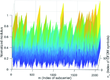
(a)

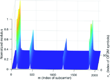
(b)

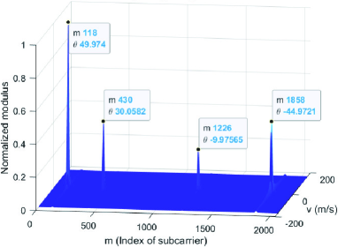
(c)

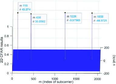
(d)

Figure 6: (a) Power spectrum of original echo signals. (b) Signal power spectrum after filtering out static environmental clutter. (c) The angle-Doppler spectrum after velocity FFT. (d) The detection results of 2D-CFAR on angle-Doppler spectrum. The four dynamic targets are set as $(50m,50^{\circ},10m/s)$, $(120m,30^{\circ},-5m/s)$, $(200m,-10^{\circ},15m/s)$ and $(80m,-45^{\circ},8m/s)$. $[\theta_{start},\theta_{end}]=[60^{\circ},-60^{\circ}]$, $N=128$ and $M+1=2048$.

Substituting (18) into (15), the echo signal of the subcarrier $f^{d,k^{*}}_{m,\ddot{m}}$ in the $n_{s}$-th OFDM symbol is

$$\begin{split}\begin{aligned} &\widetilde{y}^{d,k^{*}}_{n_{s},m,\ddot{m}}\!\!=\frac{1}{N}\sum_{k=1}^{K}\alpha_{k}e^{j\phi{(k,n_{s},f^{d,k^{*}}_{m,\ddot{m}})}}\left[\frac{\sin(\frac{\beta(f^{d,k^{*}}_{m,\ddot{m}},\theta_{k})}{2}N)}{\sin(\frac{\beta(f^{d,k^{*}}_{m,\ddot{m}},\theta_{k})}{2})}\right]^{2}\\ &\!\!\!\!=\!\!\frac{1}{N}\!\!\sum_{k=1}^{K}\!\!\alpha_{k}e^{j\phi{(k,n_{s},f^{d,k^{*}}_{m,\ddot{m}})}}\!\!\left\{\!\!\frac{\sin\left[\frac{\pi df^{d,k^{*}}_{m,\ddot{m}}}{c}(\sin\theta^{d,k^{*}}_{m,\ddot{m}}\!\!-\!\sin\theta_{k})N\right]}{\sin\left[\frac{\pi df^{d,k^{*}}_{m,\ddot{m}}}{c}(\sin\theta^{d,k^{*}}_{m,\ddot{m}}-\sin\theta_{k})\right]}\right\}^{2}\\ &\!\!\!\!=\!\!\frac{\!\alpha_{k^{*}}\!e^{\!j\!\phi{\!(k^{*}\!,\!n_{s}\!,\!f^{d,k^{*}}_{m,\ddot{m}}\!)}}}{N}\!\!\!\left\{\!\!\frac{\sin\!\!\left[\!\!\frac{\pi df^{d,k^{*}}_{m,\ddot{m}}}{c}\!(\sin\theta^{d,k^{*}}_{m,\ddot{m}}\!\!-\!\sin\!\theta_{k^{*}}\!\!)N\!\!\right]}{\sin\!\!\left[\!\!\frac{\pi df^{d,k^{*}}_{m,\ddot{m}}}{c}(\sin\theta^{d,k^{*}}_{m,\ddot{m}}\!\!-\!\sin\theta_{k^{*}})\!\right]}\!\!\!\right\}^{2}\!\!\!\!\!+\!\mathcal{\ddot{I}}(n_{s}\!,\!f^{d,k^{*}}_{m,\ddot{m}}),\end{aligned}\end{split}$$ (19)

where $e^{j\phi{(k,n_{s},f^{d,k^{*}}_{m,\ddot{m}})}}=e^{j\frac{4\pi f_{0}v_{k}}{c}n_{s}T_{s}}e^{-j\frac{4\pi f^{d,k^{*}}_{m,\ddot{m}}r_{k}}{c}}$, $e^{j\phi{(k^{*},n_{s},f^{d,k^{*}}_{m,\ddot{m}})}}=e^{j\frac{4\pi f_{0}v_{k^{*}}}{c}n_{s}T_{s}}e^{-j\frac{4\pi f^{d,k^{*}}_{m,\ddot{m}}r_{k^{*}}}{c}}$, and

$$\begin{split}\begin{aligned} &\mathcal{\ddot{I}}(n_{s},f^{d,k^{*}}_{m,\ddot{m}})\\ &=\!\!\frac{1}{N}\!\!\!\!\sum_{k=1,k\neq k^{*}}^{K}\!\!\!\!\!\!\!\!\!\alpha_{k}e^{j\phi{(k,n_{s},f^{d,k^{*}}_{m,\ddot{m}})}}\!\!\left\{\!\frac{\sin\!\!\left[\!\!\frac{\pi df^{d,k^{*}}_{m,\ddot{m}}}{c}(\sin\theta^{d,k^{*}}_{m,\ddot{m}}\!\!-\!\sin\theta_{k})N\right]}{\sin\left[\frac{\pi df^{d,k^{*}}_{m,\ddot{m}}}{c}(\sin\theta^{d,k^{*}}_{m,\ddot{m}}\!\!-\!\sin\theta_{k})\right]}\!\right\}^{2}\!\!\end{aligned}\end{split}$$ (20)

is the interference term of the other $K-1$ targets to the $k^{*}$-th target. For massive MIMO systems with sufficiently large $N$, we have $\mathcal{\ddot{I}}(n_{s},f^{d,k^{*}}_{m,\ddot{m}})\approx 0$, as long as $\theta^{d,k^{*}}_{m,\ddot{m}}\neq\theta_{k}$ in $\mathcal{\ddot{I}}(n_{s},f^{d,k^{*}}_{m,\ddot{m}})$[44]. In addition, noticing $\theta^{d,k^{*}}_{m,0}=\theta_{k^{*}}$ and $f^{d,k^{*}}_{m}=f^{d,k^{*}}_{m,0}$, we can obtain from (19) that

$$\widetilde{y}^{d,k^{*}}_{n_{s},m} =\widetilde{y}^{d,k^{*}}_{n_{s},m,0}\!\approx\!\alpha_{k^{*}}Ne^{\!j\!\frac{4\pi f_{0}v_{k^{*}}}{c}n_{s}T_{s}}e^{-j\frac{4\pi f^{d,k^{*}}_{m}r_{k^{*}}}{c}},$$ (21)

$$g^{d,k^{*}}_{n_{s},m} =\left|\widetilde{y}^{d,k^{*}}_{n_{s},m}\right|\approx\alpha_{k^{*}}N,$$ (22)

$$\varphi^{d,k^{*}}_{n_{s},m,\ddot{m}} =\!\arg\{\!\widetilde{y}^{d,k^{*}}_{n_{s},m,\ddot{m}}\}\!\approx\!\frac{4\pi\!f_{0}v_{k^{*}}n_{s}\!T_{s}}{c}\!-\!\frac{4\pi\!f^{d,k^{*}}_{m,\ddot{m}}r_{k^{*}}}{c},$$ (23)

where $\widetilde{y}^{d,k^{*}}_{n_{s},m}$ and $g^{d,k^{*}}_{n_{s},m}$ represent the complex echo signal and the echo signal power of the subcarrier $f^{d,k^{*}}_{m}$ in the $n_{s}$-th OFDM symbol respectively, while $\varphi^{d,k^{*}}_{n_{s},m,\ddot{m}}$ represents the theoretical phase of the subcarrier $f^{d,k^{*}}_{m,\ddot{m}}$ in the $n_{s}$-th symbol.

It is clear from (22) that the power of the subcarrier $f^{d,k^{*}}_{m}$ is a peak value in the power spectrum vector $\mathbf{g}_{n_{s}}$, and we call this subcarrier a peak power subcarrier. Under noiseless conditions, the frequency of the peak power subcarriers corresponding to the same target detected by the BS from $\mathbf{g}_{n_{s}}$ within each OFDM symbol ($n_{s}=0,1,2,...,N_{s}-1$) should be the same. Therefore, in noisy environments, the BS should detect a unique peak power subcarrier corresponding to a certain target from the dynamic echo matrix $\mathbf{Y}_{dynamic}$. For this effect, by performing an $N_{s}$-point Fast Fourier Transform (FFT), i.e., a velocity FFT, on each column of $\mathbf{Y}_{dynamic}$, and by moving the zero frequency component of the transformed spectrum to the center of the array, the Angle-Doppler spectrum of the echo signal can be obtained as ${\rm\mathbf{Y}}_{AD}={\rm FFTshift}\{{\rm FFT}\{\mathbf{Y}_{dynamic},N,1\},N,1\}$. The corresponding Angle-Doppler power spectrum is represented as ${\rm\mathbf{G}}_{AD}$, which satisfies $[{\rm\mathbf{G}}_{AD}]_{n_{s},m}=|[{\rm\mathbf{Y}}_{AD}]_{n_{s},m}|$. Then by performing two-dimensional Constant False Alarm Rate (CFAR) detection on ${\rm\mathbf{G}}_{AD}$, $K$ peak values can be detected corresponding to $K$ dynamic targets one by one, and the frequency of the unique peak power subcarrier corresponding to the $k^{*}$-th dynamic target can be obtained as $f^{d,k^{*}}_{m}$ from the 2D detection results. Therefore, when the BS receives the echo signal and detects the subcarrier with the peak power, the angle estimation result of the $k^{*}$-th dynamic target can be obtained by solving $\beta(f^{d,k^{*}}_{m},\theta_{k^{*}})=0$ as

$$\begin{split}\begin{aligned} \!\!\!\!\!\!\!\sin{\hat{\theta}}_{k^{*}}\!\!=\!\!\frac{(W\!\!-\!\widetilde{f}^{d,k^{*}}_{m})f_{0}}{Wf^{d,k^{*}}_{m}}\!\sin\theta_{start}\!+\!\frac{(W\!\!+\!f_{0})\widetilde{f}^{d,k^{*}}_{m}}{Wf^{d,k^{*}}_{m}}\!\sin\theta_{end}.\end{aligned}\end{split}$$ (24)

We record the frequencies of the peak power subcarriers corresponding to $K$ dynamic targets as $\{f^{d,1^{*}}_{m},f^{d,2^{*}}_{m},...,f^{d,K^{*}}_{m}\}$. Then the angle estimation of all the $K$ dynamic targets $\{\hat{\theta}_{1},\hat{\theta}_{2},...,\hat{\theta}_{K}\}$ can subsequently be determined through (24).

Fig. 6 shows an example of static clutter filtering, Angle-Doppler spectrum estimation, 2D-CFAR detection, and dynamic target angle estimation processes mentioned above, where four dynamic targets are set as $(50m,50^{\circ},10m/s)$, $(120m,30^{\circ},-5m/s)$, $(200m,-10^{\circ},15m/s)$ and $(80m,-45^{\circ},8m/s)$. It can be seen from Fig. 6(a) that the original echo signal carries a large amount of clutter caused by the static environment. After performing mean phasor cancellation, Fig. 6(b) retains almost only those echoes caused by the dynamic targets, and the angle information of the dynamic target is directly related to the frequency of the peak power subcarrier. After performing a velocity FFT on the complex signal in Fig. 6(b), four peaks corresponding to four dynamic targets can be clearly observed in the Angle-Doppler spectrum shown in Fig. 6(c), which can also be observed in the 2D-CFAR detection results shown in Fig. 6(d). According to the peak power subcarriers and (24), the angle estimates corresponding to the dynamic targets can be obtained as $49.974^{\circ}$, $30.0582^{\circ}$, $-9.97565^{\circ}$ and $-44.9721^{\circ}$.

Next, to estimate the distance and velocity of dynamic target, let us name the $2\ddot{M}+1$ subcarriers around the peak power subcarrier $f^{d,k^{*}}_{m}$ peak sidelobe subcarriers, mark the subcarrier with frequency $f^{d,k^{*}}_{m}$ as $m_{k^{*}}$, and regard $2\ddot{M}+1$ as the sidelobe window width. Then the echo signal matrix of the $2\ddot{M}+1$ peak sidelobe subcarriers corresponding to the $k^{*}$-th target within $N_{s}$ OFDM symbols can be extracted from $\mathbf{Y}_{dynamic}$ and are represented as $\mathbf{Y}_{RD,k^{*}}=\mathbf{Y}_{dynamic}[:,m_{k^{*}}-\ddot{M}:m_{k^{*}}+\ddot{M}]\in\mathbb{C}^{N_{s}\times(2\ddot{M}+1)}$. It is seen from (23) that the echo signals on these sidelobe subcarriers carry the distance and velocity information of the $k^{*}$-th dynamic target.

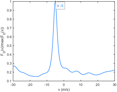
(a)

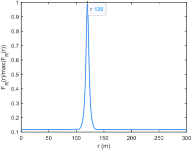
(b)

Figure 7: (a) An example of estimating dynamic target velocity based on the MUSIC algorithm. (b) An example of estimating dynamic target distance based on the MUSIC algorithm. The target is set as $(120m,30^{\circ},-5m/s)$ and SNR $=0$ dB.

Specifically, we normalize each element in $\mathbf{Y}_{RD,k^{*}}$ to obtain a new sidelobe subcarrier echo signal matrix $\mathbf{\bar{Y}}_{RD,k^{*}}$, which satisfies $[\mathbf{\bar{Y}}_{RD,k^{*}}]_{i,j}=\frac{[\mathbf{Y}_{RD,k^{*}}]_{i,j}}{|[\mathbf{Y}_{RD,k^{*}}]_{i,j}|}$. According to (19) and (23), $\mathbf{\bar{Y}}_{RD,k^{*}}$ can be represented in detail as

$$\begin{split}\begin{aligned} &\!\!\!\!\mathbf{\bar{Y}}_{RD,k^{*}}\!\!=\!e^{-j\frac{4\pi f^{d,k^{*}}_{m,-\ddot{M}}r_{k^{*}}}{c}}\times\\ &\begin{bmatrix}e^{\!j\frac{\!4\!\pi\!f_{0}v_{k^{*}}T_{s}}{c}0}e^{-j\frac{4\pi r_{k^{*}}\Delta f}{c}0}&\!\!\!\!\cdots\!\!\!\!&e^{\!j\!\frac{\!4\!\pi\!f_{0}\!v_{k^{*}}\!T_{s}}{c}0}e^{-j\frac{4\pi r_{k^{*}}\Delta f}{c}(2\ddot{M})}\\ \vdots&\ddots&\vdots\\ e^{\!j\!\frac{4\!\pi\!f_{0}\!v_{k^{*}}\!T_{s}}{c}\!(\!N_{s}\!-\!1\!)}\!e^{\!-\!j\!\frac{4\pi r_{k^{*}}\!\Delta\!f}{c}\!0}&\!\!\!\!\cdots\!\!\!\!&\!\!e^{\!j\!\frac{\!4\!\pi\!f_{0}\!v_{k^{*}}\!T_{s}}{c}\!(\!N_{s}\!-\!1\!)}\!e^{\!-\!j\frac{\!4\pi r_{k^{*}}\!\Delta\!f}{c}(2\ddot{M})}\\ \end{bmatrix}.\end{aligned}\end{split}$$ (25)

We define the Doppler steering vector in the $N_{s}$ dimensions and the distance steering vector in the $2\ddot{M}+1$ dimensions as $\mathbf{k}_{D}(v_{k^{*}})=[1,e^{j\frac{4\pi f_{0}v_{k^{*}}T_{s}}{c}},...,e^{j\frac{4\pi f_{0}v_{k^{*}}T_{s}}{c}(N_{s}-1)}]^{T}\in\mathbb{C}^{N_{s}\times 1}$ and $\mathbf{k}_{R}(r_{k^{*}})=[1,e^{-j\frac{4\pi r_{k^{*}}\Delta f}{c}},...,e^{-j\frac{4\pi r_{k^{*}}\Delta f}{c}(2\ddot{M})}]^{T}\in\mathbb{C}^{(2\ddot{M}+1)\times 1}$, respectively. Then $\mathbf{\bar{Y}}_{RD,k^{*}}$ and its transpose matrix can be further represented as

$$\begin{split}\begin{aligned} \mathbf{\bar{Y}}_{RD,k^{*}}=e^{-j\frac{4\pi f^{d,k^{*}}_{m,-\ddot{M}}r_{k^{*}}}{c}}\mathbf{k}_{D}(v_{k^{*}})\mathbf{k}^{T}_{R}(r_{k^{*}}),\end{aligned}\end{split}$$ (26)

$$\begin{split}\begin{aligned} \mathbf{\bar{Y}}^{T}_{RD,k^{*}}=e^{-j\frac{4\pi f^{d,k^{*}}_{m,-\ddot{M}}r_{k^{*}}}{c}}\mathbf{k}_{R}(r_{k^{*}})\mathbf{k}^{T}_{D}(v_{k^{*}}).\end{aligned}\end{split}$$ (27)

From (26) and (27), it can be seen that $\mathbf{\bar{Y}}_{RD,k^{*}}$ and $\mathbf{\bar{Y}}^{T}_{RD,k^{*}}$ are the generalized array signal forms for Doppler steering array and range steering array. Hence the velocity and distance of the $k^{*}$-th dynamic target can be estimated from the autocorrelation matrices of $\mathbf{\bar{Y}}_{RD,k^{*}}$ and $\mathbf{\bar{Y}}^{T}_{RD,k^{*}}$, as

$$\begin{split}\begin{aligned} \mathbf{R}^{X}_{D,k^{*}}=\frac{1}{2\ddot{M}+1}\mathbf{\bar{Y}}_{RD,k^{*}}(\mathbf{\bar{Y}}_{RD,k^{*}})^{H},\end{aligned}\end{split}$$ (28)

$$\begin{split}\begin{aligned} \mathbf{R}^{X}_{R,k^{*}}=\frac{1}{N_{s}}\mathbf{\bar{Y}}^{T}_{RD,k^{*}}(\mathbf{\bar{Y}}^{T}_{RD,k^{*}})^{H}.\end{aligned}\end{split}$$ (29)

We here adopt the reliable multiple signal classification (MUSIC) algorithm to solve the generalized array signal estimation problem. We decompose the eigenvalues of $\mathbf{R}^{X}_{D,k^{*}}$ and $\mathbf{R}^{X}_{R,k^{*}}$ to obtain the diagonal matrix with eigenvalues ranging from large to small ($\mathbf{\Sigma}_{D,k^{*}}$ and $\mathbf{\Sigma}_{R,k^{*}}$) and the corresponding eigenvector matrix ($\mathbf{U}_{D,k^{*}}$ and $\mathbf{U}_{R,k^{*}}$). That is

$$\begin{split}\begin{aligned} [\mathbf{U}_{D,k^{*}},\mathbf{\Sigma}_{D,k^{*}}]={\rm eig}(\mathbf{R}^{X}_{D,k^{*}}),\end{aligned}\end{split}$$ (30)

$$\begin{split}\begin{aligned} [\mathbf{U}_{R,k^{*}},\mathbf{\Sigma}_{R,k^{*}}]={\rm eig}(\mathbf{R}^{X}_{R,k^{*}}).\end{aligned}\end{split}$$ (31)

Then the Minimum Description Length (MDL) criterion is utilized to estimate the number of dynamic targets from $\mathbf{\Sigma}_{D,k^{*}}$ and $\mathbf{\Sigma}_{R,k^{*}}$ as $N_{k^{*},D}^{MDL}$ and $N_{k^{*},R}^{MDL}$ respectively, and we define $N_{k^{*}}^{MDL}={\rm min}\{N_{k^{*},D}^{MDL},N_{k^{*},R}^{MDL}\}$ as the number of dynamic targets to be estimated from $\mathbf{\bar{Y}}_{RD,k^{*}}$. Under normal circumstances, there is always $N_{k^{*},D}^{MDL}=N_{k^{*},R}^{MDL}$. Due to the assumption that the angles of each dynamic target are different from each other, there will be $N_{k^{*}}^{MDL}=1$. Therefore, the noise space related to the velocity array can be represented as $\mathbf{U}^{N}_{D,k^{*}}=\mathbf{U}_{D,k^{*}}[:,N_{k^{*}}^{MDL}+1:N_{s}]$, and the noise space related to the distance array can be represented as $\mathbf{U}^{N}_{R,k^{*}}=\mathbf{U}_{R,k^{*}}[:,N_{k^{*}}^{MDL}+1:2\ddot{M}+1]$. Then the Doppler spectral function with search velocity $v$ and the distance spectral function with search distance $r$ for the $k^{*}$-th dynamic target are

$$\begin{split}\begin{aligned} F_{D,k^{*}}(v)=\frac{1}{\mathbf{k}^{H}_{D}(v)\mathbf{U}^{N}_{D,k^{*}}(\mathbf{U}^{N}_{D,k^{*}})^{H}\mathbf{k}_{D}(v)},\end{aligned}\end{split}$$ (32)

$$\begin{split}\begin{aligned} F_{R,k^{*}}(r)=\frac{1}{\mathbf{k}^{H}_{R}(r)\mathbf{U}^{N}_{R,k^{*}}(\mathbf{U}^{N}_{R,k^{*}})^{H}\mathbf{k}_{R}(r)}.\end{aligned}\end{split}$$ (33)

Then the velocity and distance estimation results of the $k^{*}$-th target can be obtained by searching the maximum values of $F_{D,k^{*}}(v)$ and $F_{R,k^{*}}(r)$ , i.e,

$$\begin{split}\begin{aligned} \!\!\!\!\hat{v}_{k^{*}}\!=\!\mathop{\arg\max}\limits_{v}F_{D,k^{*}}(v),\end{aligned}\end{split}$$ (34)

$$\begin{split}\begin{aligned} \!\!\!\!\hat{r}_{k^{*}}\!=\!\mathop{\arg\max}\limits_{r}F_{R,k^{*}}(r).\end{aligned}\end{split}$$ (35)

Since the CBS-Beamforming can cover the entire sensing area in one beam sweep, the proposed dynamic target sensing scheme with (24), (34) and (35) only needs one beam sweep to obtain the angle, distance and velocity estimations for all the dynamic targets, which we term You Only Listen Once (YOLO for short).

Fig. 7 shows an example of the estimation of target velocity and distance with YOLO, in which the target is one of the four targets in Fig. 6 and is set as $(120m,30^{\circ},-5m/s)$. According to the frequency of the peak power subcarrier in Fig. 6 and (24), this target angle can be estimated as $30.0582^{\circ}$. Then according to (34) and (35), the velocity and distance estimates of this target can be clearly obtained from Fig. 7 as $-5m/s$ and $120m$, respectively.

IV-B Multiple YOLO: An Improved Localization Scheme

Although the proposed YOLO algorithm is theoretically valid, its performance under noise may not be satisfactory. The basic idea of target distance and velocity estimation in YOLO is to use the phase differences of the $2\ddot{M}+1$ sidelobe subcarriers with different frequencies and $N_{s}$ continuous OFDM symbols in only one beam sweep. However, it can be seen from (19) that the power of the $k^{*}$-th target’s sidelobe subcarriers is smaller than that of the peak power subcarrier. Hence the other $K-1$ targets will cause relatively higher interference to the $k^{*}$-th target’s sidelobe subcarriers than its peak power subcarrier, which may lead to a non-zero error floor for distance and velocity estimation. Conversely, the peak power subcarrier contains more pure and accurate target distance and velocity information than sidelobe subcarriers.

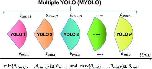
Figure 8: Schematic diagram of MYOLO scheme.

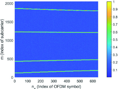
(a)

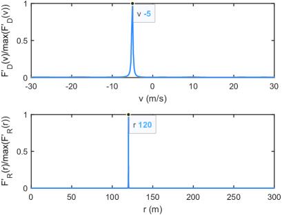
(b)

Figure 9: (a) An example of the power map in MYOLO, in which the four targets are set as $(50m,50^{\circ},10m/s)$, $(120m,30^{\circ},-5m/s)$, $(200m,-10^{\circ},15m/s)$ and $(80m,-45^{\circ},8m/s)$. (b) An example of velocity and distance estimation spectra in MYOLO, which refers to the dynamic target with parameter $(120m,30^{\circ},-5m/s)$. SNR $=0$ dB, $N=128$, $M=2048$ and $P=10$.

Hence we consider listening more times to improve the sensing performance. However, directly repeating YOLO for many times cannot improve the performance much, because of the interference of the sidelobe subcarriers in YOLO. We thus design a new method based on $P$-times beam sweeping with different CBS-Beamforming ranges to realize higher precision target sensing as shown in Fig. 8, in which we only retain the information of the peak power subcarrier while discarding the sidelobe subcarriers. By doing this, we set every time beam sweeping as a YOLO but with different beam squint range. Specifically, we set the start angle as $\theta_{start,p}$ and the end angle as $\theta_{end,p}$ for the $p$-th beam sweep, where $p=1,2,...,P$. Note that there should be $\min\{\theta_{start,1},\theta_{start,2},...,\theta_{start,P}\}\geq\theta_{start}$ and $\max\{\theta_{end,1},\theta_{end,2},...,\theta_{end,P}\}\leq\theta_{end}$, such that each beam sweep can cover the whole sensing range.

Within each beam sweep, the BS can always detect $K$ peak power subcarriers in the echo power spectrum matrix $\mathbf{G}_{p}$, whose frequencies are denoted by $\{f^{d,1^{*},p}_{m},f^{d,2^{*},p}_{m},...,f^{d,K^{*},p}_{m}\}$. The angle estimates of the $K$ targets can be calculated through (24) as $\{\hat{\theta}_{1^{*},p},\hat{\theta}_{2^{*},p},...,\hat{\theta}_{K^{*},p}\}$. In addition, the echo signal after mean phase cancellation of the peak power subcarrier $f^{d,k^{*},p}_{m}$ within the $n_{s}$-th OFDM symbol time can be written as $\widetilde{y}^{d,k^{*},p}_{n_{s},m}$, where ${\rm arg}\{\widetilde{y}^{d,k^{*},p}_{n_{s},m}\}\approx\frac{4\pi f_{0}v_{k^{*}}n_{s}T_{s}}{c}-\frac{4\pi f^{d,k^{*},p}_{m}r_{k^{*}}}{c}$ can be derived from (23). Then the received signals of all peak power subcarriers within all OFDM symbols can be represented as $\{\widetilde{y}^{d,1^{*},p}_{0,m},...,\widetilde{y}^{d,1^{*},p}_{(N_{s}-1),m};...;\widetilde{y}^{d,2^{*},p}_{0,m},...,\widetilde{y}^{d,2^{*},p}_{(N_{s}-1),m}\}$.

After $P$-times beam sweep, we can combine the power spectrum matrices $\left\{\mathbf{G}_{1},\mathbf{G}_{2},...,\mathbf{G}_{P}\right\}$ into a larger two-dimensional matrix, called the power map. Since the frequencies of the $P$ peak power subcarriers corresponding to the same target are adjacent, we can build the following three information vectors or matrix corresponding to the $k^{*}$-th target as

$$\mathbf{f}^{d}_{k^{*}} =[f^{d,k^{*},1}_{m},f^{d,k^{*},2}_{m},...,f^{d,k^{*},P}_{m}]^{T}\in\mathbb{C}^{P\times 1},$$ (36)

$$\bm{\hat{\theta}}^{d}_{k^{*}} =[\hat{\theta}_{k^{*},1},\hat{\theta}_{k^{*},2},...,\hat{\theta}_{k^{*},P}]^{T}\in\mathbb{C}^{P\times 1},$$ (37)

$$\mathbf{\widetilde{Y}}^{d}_{k^{*}} =\begin{bmatrix}\widetilde{y}^{d,k^{*},1}_{0,m}&\cdots&\widetilde{y}^{d,k^{*},P}_{0,m}\\ \vdots&\ddots&\vdots\\ \widetilde{y}^{d,k^{*},1}_{(N_{s}-1),m}&\cdots&\widetilde{y}^{d,k^{*},P}_{(N_{s}-1),m}\\ \end{bmatrix}\in\mathbb{C}^{N_{s}\times P}.$$ (38)

Fig. 9(a) shows an example of the power map, where the horizontal axis and the vertical axis are the indices of OFDM symbols and subcarriers respectively, and the dynamic targets’ parameters are consistent with the settings in Fig. 6. It is seen that the peak power subcarriers corresponding to the same target approximately formulate a line. Moreover, the number of the lines is $4$, which indicates that there are four dynamic targets within the sensing range.

For angle estimation, we can take the average value of $\bm{\hat{\theta}}^{d}_{k^{*}}$ as the final angle estimation of the $k^{*}$-th target, i.e.

$$\begin{split}\begin{aligned} \hat{\theta}_{k^{*}}=\frac{1}{P}\sum_{p=1}^{P}\hat{\theta}_{k^{*},p}.\end{aligned}\end{split}$$ (39)

In addition, note that the frequencies of the $P$ peak power subcarriers corresponding to the $k^{*}$-th target are different thanks to the slightly different range of beam squint at each time beam sweeping. Hence we can still estimate the distances and velocities of the dynamic targets using the phase differences of the echo signals from different frequency subcarriers within different OFDM symbols. Specifically, we normalize each element in $\mathbf{\widetilde{Y}}^{d}_{k^{*}}$ to obtain a new peak power subcarrier echo signal matrix $\mathbf{\bar{Y}}^{d}_{k^{*}}$, which satisfies $[\mathbf{\bar{Y}}^{d}_{k^{*}}]_{i,j}=\frac{[\mathbf{\widetilde{Y}}^{d}_{k^{*}}]_{i,j}}{|[\mathbf{\widetilde{Y}}^{d}_{k^{*}}]_{i,j}|}$. Since the phase of $\mathbf{\bar{Y}}^{d}_{k^{*}}$ in (38) is still linearly uniform in the Doppler dimension, the Doppler steering vector in the $N_{s}$ dimension is still defined as $\mathbf{k}_{D,k^{*}}(v)=[1,e^{j\frac{4\pi f_{0}vT_{s}}{c}},...,e^{j\frac{4\pi f_{0}vT_{s}}{c}(N_{s}-1)}]^{T}\in\mathbb{C}^{N_{s}\times 1}$. However, because the phase of $\mathbf{\bar{Y}}^{d}_{k^{*}}$ is non-uniform in the distance dimension, it is necessary to define the distance steering vector corresponding to the $k^{*}$-th target as $\mathbf{k}_{R,k^{*}}(r)=[1,e^{-j\frac{4\pi r}{c}(f_{m}^{d,k^{*},2}-f_{m}^{d,k^{*},1})},...,e^{-j\frac{4\pi r}{c}(f_{m}^{d,k^{*},P}-f_{m}^{d,k^{*},1})}]^{T}\in\mathbb{C}^{P\times 1}$. Then $\mathbf{\bar{Y}}^{d}_{k^{*}}$ and its transpose can be represented as $\mathbf{\bar{Y}}^{d}_{k^{*}}=e^{-j\frac{4\pi f_{m}^{d,k^{*},1}r_{k^{*}}}{c}}\mathbf{k}_{D,k^{*}}(v_{k^{*}})\mathbf{k}^{T}_{R,k^{*}}(r_{k^{*}})$ and $(\mathbf{\bar{Y}}^{d}_{k^{*}})^{T}=e^{-j\frac{4\pi f_{m}^{d,k^{*},1}r_{k^{*}}}{c}}\mathbf{k}_{R,k^{*}}(r_{k^{*}})\mathbf{k}^{T}_{D,k^{*}}(v_{k^{*}})$. Similar to (28) to (35), we calculate the covariance matrix of the peak power subcarrier signals as $\mathbf{R}^{X^{\prime}}_{D,k^{*}}$ and $\mathbf{R}^{X^{\prime}}_{R,k^{*}}$, perform eigenvalue decomposition to obtain $\mathbf{U}^{\prime}_{D,k^{*}}$, $\mathbf{\Sigma}^{\prime}_{D,k^{*}}$, $\mathbf{U}^{\prime}_{R,k^{*}}$ and $\mathbf{\Sigma}^{\prime}_{R,k^{*}}$, and extract the noise subspaces as $\mathbf{U}^{N^{\prime}}_{D,k^{*}}$ and $\mathbf{U}^{N^{\prime}}_{R,k^{*}}$. Then the velocity and distance estimates of the $k^{*}$-th target can be obtained as

$$\begin{split}\begin{aligned} \!\!\!\!\hat{v}_{k^{*}}\!&=\!\mathop{\arg\max}\limits_{v}F^{\prime}_{D,k^{*}}(v)\\ &=\mathop{\arg\max}\limits_{v}\frac{1}{\mathbf{k}^{H}_{D,k^{*}}(v)\mathbf{U}^{N^{\prime}}_{D,k^{*}}(\mathbf{U}^{N^{\prime}}_{D,k^{*}})^{H}\mathbf{k}_{D,k^{*}}(v)},\end{aligned}\end{split}$$ (40)

$$\begin{split}\begin{aligned} \!\!\!\!\hat{r}_{k^{*}}\!&=\!\mathop{\arg\max}\limits_{r}F^{\prime}_{R,k^{*}}(r)\\ &=\mathop{\arg\max}\limits_{r}\frac{1}{\mathbf{k}^{H}_{R,k^{*}}(r)\mathbf{U}^{N^{\prime}}_{R,k^{*}}(\mathbf{U}^{N^{\prime}}_{R,k^{*}})^{H}\mathbf{k}_{R,k^{*}}(r)}.\end{aligned}\end{split}$$ (41)

Different from YOLO, the steps from (39) to (41) utilize the correlation among the peak power subcarriers corresponding to the same target in $P$-times beam sweeping to sense the target, which is termed Multiple-YOLO (MYOLO for short). MYOLO greatly reduces the interference among multiple targets, which not only improves the sense accuracy, but also eliminates the need to allocate $2\ddot{M}+1$ sidelobe subcarriers for each target as did in YOLO. Hence MYOLO can support the sensing of more targets than YOLO under the same configuration. Meanwhile, the selection of $P$ provides a tradeoff between the time required for sensing and the sensing performance.

For example, Fig. 9(b) shows the $v$-$F^{\prime}_{D}(v)$ and $r$-$F^{\prime}_{R}(r)$ curves of searching the velocity and distance for the dynamic target with $(120m,30^{\circ},-5m/s)$. According to the peak value of each search curve, the estimation results of velocity and distance for this target can be seen as $-5m/s$ and $120m$. Comparing Fig. 9(b) and Fig. 7, we can see that the peak of the spectrum search curves in MYOLO are narrower than those of YOLO, which indicates that MYOLO can better isolate the mutual interference among multiple targets.

IV-C Complexity analysis

In the YOLO scheme, the computational complexity mainly comes from the eigenvalue decomposition of $\mathbf{R}^{X}_{D,k^{*}}$ and $\mathbf{R}^{X}_{R,k^{*}}$. Thus the total computational complexity of the YOLO scheme is $\mathcal{O}\left(N_{s}^{3}+(2\ddot{M}+1)^{3}\right)$. Similarly, the computational complexity of the MYOLO scheme mainly comes from the eigenvalue decomposition of $\mathbf{R}^{X^{\prime}}_{D,k^{*}}$ and $\mathbf{R}^{X^{\prime}}_{R,k^{*}}$. Thus the total computational complexity of the MYOLO scheme can be expressed as $\mathcal{O}\left(N_{s}^{3}+P^{3}\right)$.

V Simulation Results

In our simulations, we set the number of antennas as $N=128$, the lowest carrier frequency as $f_{0}$ = 220 GHz and $d=\frac{1}{2}\lambda$. We assume that the required sensing range of the BS is $[\theta_{start},\theta_{end}]=[60^{\circ},-60^{\circ}]$. The noise is assumed to obey the complex Gaussian distribution with mean $\mu=0$ and variance $\sigma_{n}^{2}=1$. The root mean square errors (RMSEs) of angle estimation, distance estimation, and velocity estimation are defined as ${\rm RMSE}_{\theta}=\sqrt{\frac{\sum_{i=1}^{Count}(\hat{\theta}_{s(i)}-\theta_{s})^{2}}{Count}}$, ${\rm RMSE}_{r}=\sqrt{\frac{\sum_{i=1}^{Count}(\hat{r}_{s(i)}-r_{s})^{2}}{Count}}$, and ${\rm RMSE}_{v}=\sqrt{\frac{\sum_{i=1}^{Count}(\hat{v}_{s(i)}-v_{s})^{2}}{Count}}$, where $Count$ is the number of repeated experiments, the true parameters of the dynamic target are $(r_{s},\theta_{s},v_{s})$, and $(\hat{r}_{s(i)},\hat{\theta}_{s(i)},\hat{v}_{s(i)})$ are the estimated parameters of the target.

V-A Dynamic Target Sensing Performance

Assume that the transmission bandwidth is $W=1$ GHz, the number of OFDM symbols is $N_{s}=32$, and the number of subcarriers is $M+1=2048$. In the YOLO scheme, we set the range of beam squint as $[\theta_{start},\theta_{end}]=[60^{\circ},-60^{\circ}]$ and the sidelobe window width as $2\ddot{M}+1=21$. In the MYOLO scheme, we set $P=8$, $\theta_{start,p}=60^{\circ},61^{\circ},62^{\circ},...,67^{\circ}$, and $\theta_{end,p}=-\theta_{start,p}=-60^{\circ},-61^{\circ},-62^{\circ},...,-67^{\circ}$. Fig. 10 shows the RMSEs of dynamic target sensing versus signal-to-noise ratio (SNR).

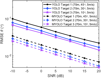
(a)

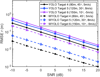
(b)

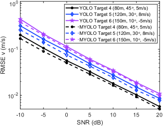
(c)

Figure 10: (a) Angle sensing RMSE performance results. (b) Distance sensing RMSE performance results. (c) Velocity sensing RMSE performance results.

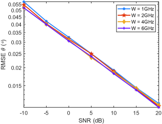
(a)

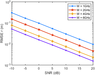
(b)

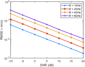
(c)

Figure 11: (a) The angle sensing RMSE for different bandwidths. (b) The distance sensing RMSE for different bandwidths. (c) The velocity sensing RMSE for different bandwidths. The single dynamic target is set as $(200m,10^{\circ},5m/s)$.

It can be seen from Fig. 10(a) that $\rm RMSE_{\theta}$ keeps decreasing as SNR increases. For the YOLO scheme, the average $\rm RMSE_{\theta}$ is $0.08^{\circ}$ when SNR is $-10$ dB, and reaches $0.02^{\circ}$ when SNR increases to $15$ dB. Comparing the curves corresponding to different targets, we find that the closer the target is to $0^{\circ}$, the lower the $\rm RMSE_{\theta}$ will be. This phenomenon is due to the non-uniformity of the angle distribution of the beam squint in CBS-beamforming as shown in Fig. 4(b). It can be seen from (12) that there are more subcarriers distributed around $0^{\circ}$, and thus the angle spacing between adjacent subcarriers is smaller, which means that the angle sensing error will also be smaller around $0^{\circ}$. In addition, by comparing the solid line and the dotted line, we see that MYOLO has better angle sensing performance than YOLO.

Fig. 10(b) and Fig. 10(c) show the ${\rm RMSE}_{r}$ and ${\rm RMSE}_{v}$ for different targets. It is seen from them that both the ${\rm RMSE}_{r}$ and ${\rm RMSE}_{v}$ decrease as the SNR increases, and the ${\rm RMSE}_{r}$ and ${\rm RMSE}_{v}$ of the target is larger if the target is father away. More importantly, by comparing the solid line and the dotted line, we can see that when other conditions are the same, the MYOLO scheme has higher distance estimation accuracy and velocity estimation accuracy than the YOLO scheme. This is because MYOLO reduces the mutual interference among multiple targets at the expense of more sensing time.

V-B Influence of Bandwidth $W$

In a practical Terahertz ISAC system, only partial spectrum resources are used for sensing, while other spectrum resources are used for communications. Therefore, we consider changing $W$ to explore the impact of bandwidth. Fig. 11 shows the sensing RMSEs of the YOLO scheme when a single dynamic target is set as $(200m,10^{\circ},5m/s)$, while the bandwidth varies. As $W$ decreases, the ${\rm RMSE}_{\theta}$ is almost unchanged, while the ${\rm RMSE}_{r}$ gradually increases. This is consistent with the basic intuition that the accuracy of distance estimation in radar system increases with the increase of system bandwidth, while the angle estimation accuracy is almost independent of the bandwidth. In addition, due to the fixed number of subcarriers $M+1$ in the experiment, as the bandwidth $W$ increases, the frequency interval between subcarriers $\Delta f$ gradually increases, leading to a decrease in velocity resolution, which explains the phenomenon of ${\rm RMSE}_{v}$ increasing as $W$ increasing in Fig. 11(c).

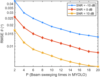
(a)

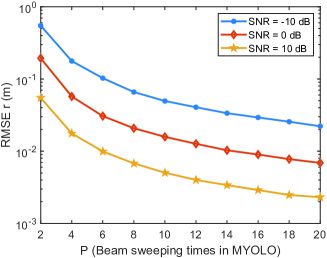
(b)

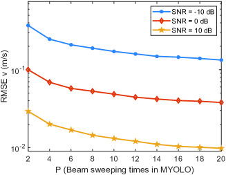
(c)

Figure 12: (a) The angle sensing MSE vs. the number of beam sweeps. (b)The distance sensing MSE vs. the number of beam sweeps. (c)The velocity sensing MSE vs. the number of beam sweeps.

V-C Influence of Beam Sweeping Times $P$

We study the effect of changing $P$ in the MYOLO sensing scheme. It can be seen from Fig. 12(a) that the ${\rm RMSE}_{\theta}$ decreases with the increase of $P$. When $P=4$ and SNR $=10$ dB, the ${\rm RMSE}_{\theta}$ is $0.011^{\circ}$, while when $P$ increases to $12$, the ${\rm RMSE}_{\theta}$ decreases to $0.007^{\circ}$. This is mainly because MYOLO’s angle estimation method, formula (39), takes the mean value of the angle estimation results obtained from $P$ times YOLO scheme. Therefore, the angle estimation accuracy will improve as $P$ increases.

It can be seen from Fig. 12(b) that the ${\rm RMSE}_{r}$ decreases with the increase of $P$. When $P=4$ and SNR $=10$ dB, the ${\rm RMSE}_{r}$ is $0.017m$, while when $P$ increases to $12$, the ${\rm RMSE}_{r}$ decreases to $0.005m$. This is mainly because in the MYOLO scheme, the distance array represented by the distance steering vector increases with the increase of $P$, and the larger distance arrays are more conducive to distance estimation.

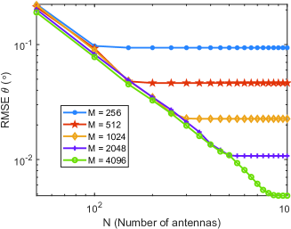
(a)

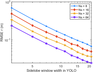
(b)

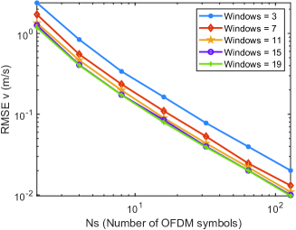
(c)

Figure 13: (a) Relationship between the angle sensing RMSE and the number of antennas $N$ and the number of subcarriers $M$. (b) Relationship between the distance sensing RMSE and the sidelobe window width $2\ddot{M}+1$ and the number of symbols $N_{s}$. (c) Relationship between the velocity sensing RMSE and the number of symbols $N_{s}$ and the sidelobe window width $2\ddot{M}+1$.

It can be seen from Fig. 12(c) that the ${\rm RMSE}_{v}$ decreases with the increase of $P$. When $P=4$ and SNR $=10$ dB, ${\rm RMSE}_{v}$ is $0.020m/s$, while when $P$ increases to $12$, the ${\rm RMSE}_{v}$ decreases to $0.012m/s$. This is mainly because in the MYOLO scheme, the number of observations on the velocity array represented by the velocity steering vector increases with the increase of $P$, and more observations make the covariance matrix calculation of the velocity array more accurate, thereby improving the accuracy of velocity estimation.

Since increasing $P$ requires more time to complete sensing, there is a tradeoff between the sensing accuracy and the acceptable sensing time.

V-D Influence of Other System Parameters

Fig. 13 shows the impact of some other system parameters on sensing performance. Fig. 13(a) shows the variation ${\rm RMSE}_{\theta}$ with the number of antennas and subcarriers. It is seen that the ${\rm RMSE}_{\theta}$ decreases with the increase of $N$. According to the theory of array signal processing, the beam width of the antenna array is inversely proportional to $2N$. Therefore, by increasing $N$, the BS can concentrate the energy in a narrower width to improve the angle sensing performance. However, it is seen that when $N$ is large enough, ${\rm RMSE}_{\theta}$ will converge to a non-zero error floor, which will decrease with the increase of the number of subcarriers $M$. The reason for this is that when $M$ is small, the distribution interval between subcarriers is large, which limits the angle sensing performance of the beams with very narrow beam width.

Fig. 13(b) shows the distance sensing RMSE in the YOLO scheme versus the sidelobe window width $2\ddot{M}+1$ and the number of OFDM symbols $N_{s}$. It can be seen from the figure that the distance RMSE gradually decreases as the width of the sidelobe window increases. This is because a larger sidelobe window width means a larger distance steering array, making distance sensing more accurate. In addition, it can be found that increasing the number of OFDM symbols can also improve the accuracy of distance sensing.

Fig. 13(c) shows the velocity sensing RMSE in the YOLO scheme versus the number of OFDM symbols $N_{s}$ and the sidelobe window width $2\ddot{M}+1$. From this figure, it can be seen that using more OFDM symbols can improve the accuracy of velocity sensing. In addition, increasing the width of the sidelobe window can also improve the accuracy of velocity sensing to a certain extent. But as the window width increases, the improvement gradually decreases.

VI Conclusions

In this paper, we have proposed the use of the beam squint effect in massive MIMO Terahertz wideband communications systems to realize non-cooperative dynamic target sensing. Specifically, we have constructed a wideband channel model for echo signals, and proposed a beamforming scheme that controls the range of beam squint by adjusting the values of PSs and TTDs, such that different subcarriers can point to different directions in a planned way. The echo signals of different subcarriers will carry target information in different directions, based on which the targets’ angles can be estimated through a sophisticatedly designed algorithm. Moreover, we have proposed a supporting method based on extended array signal estimation, which utilizes the phase changes of different frequency subcarriers within different OFDM symbols to estimate the distance and velocity of dynamic targets. Interestingly, the proposed method only needs the BS to transmit and receive the signals once to realize full spatial target localization, which means that You Only Listen Once (YOLO). In order to further improve the accuracy of sensing, we have proposed a high-precision sensing scheme based on multiple applications of YOLO, which utilized the mean estimation, non-uniform array signal estimation, and uniform array signal estimation to realize high-precision estimation of dynamic target angle, distance, and velocity, respectively. Compared with the traditional ISAC method that requires multiple beam sweeps, the proposed one can greatly reduce the sensing time overhead. Simulation results have demonstrated the effectiveness of the proposed scheme.

APPENDIX A
Proof of (15)

The echo signal after clutter filtering is $\widetilde{y}_{n_{s},m}$, which is given by (14) and the phase of the additive term in $\widetilde{y}_{n_{s},m}$ is $2\pi(\phi_{n}+\widetilde{f}_{m}t_{n}+\frac{f_{m}}{c}nd\sin\theta_{k})$. We set $\phi_{n}=-\frac{f_{0}nd\sin\theta_{start}}{c}$ and $t_{n}=-\frac{\phi_{n}}{W}-\frac{(f_{0}+W)nd\sin\theta_{end}}{Wc}$. Then we have $2\pi(\phi_{n}+\widetilde{f}_{m}t_{n}+\frac{f_{m}}{c}nd\sin\theta_{k})=-\frac{2\pi dn}{Wc}[(W\!-\!\widetilde{f}_{m})f_{0}\sin\theta_{start}+(W\!+\!f_{0})\widetilde{f}_{m}\sin\theta_{end}-Wf_{m}\sin\theta_{k}]=-n\beta(f_{m},\theta_{k})$, where $\beta(f_{m},\theta_{k})=\frac{2\pi d}{Wc}[(W-\widetilde{f}_{m})f_{0}\sin\theta_{start}+(W+f_{0})\widetilde{f}_{m}\sin\theta_{end}-Wf_{m}\sin\theta_{k}]$. Therefore (14) is simplified as

$$\begin{split}\begin{aligned} &\widetilde{y}_{n_{s},m}\\ &\approx\sum_{k=1}^{K}\!\!\left\{\!\!\frac{\alpha_{k}}{N}e^{j\phi{(k,n_{s},f_{m})}}\!\!\left[\!\!\sum_{n=-\frac{N-1}{2}}^{\frac{N-1}{2}}\!\!\!\!\!\!e^{j2\pi\phi_{n}}\!e^{j2\pi\widetilde{f}_{m}t_{n}}\!e^{j\frac{2\pi f_{m}}{c}nd\sin\theta_{k}}\right]^{2}\!\!\right\}\\ &=\sum_{k=1}^{K}\left\{\frac{\alpha_{k}}{N}e^{j\phi{(k,n_{s},f_{m})}}\times\left[\sum_{n=-\frac{N-1}{2}}^{\frac{N-1}{2}}e^{-jn\beta(f_{m},\theta_{k})}\right]^{2}\right\}\\ &=\sum_{k=1}^{K}\left\{\frac{\alpha_{k}}{N}e^{j\phi{(k,n_{s},f_{m})}}\left[\frac{\sin(\frac{\beta(f_{m},\theta_{k})}{2}N)}{\sin(\frac{\beta(f_{m},\theta_{k})}{2})}\right]^{2}\right\}.\end{aligned}\end{split}$$ (42)

This completes the proof of (15).

Hongliang Luo received the B.Eng. degree from Xidian University, Xi’an, China, in 2023. He is currently working toward the Ph.D. degree with the Department of Automation, Tsinghua University, Beijing, China. His research interests include integrated sensing and communications, wireless communications, radar sensing, array signal processing, massive MIMO and beamforimg design.

Feifei Gao (Fellow, IEEE) received the B.Eng. degree from Xi’an Jiaotong University, Xi’an, China in 2002, the M.Sc. degree from McMaster University, Hamilton, ON, Canada in 2004, and the Ph.D. degree from National University of Singapore, Singapore in 2007. Since 2011, he joined the Department of Automation, Tsinghua University, Beijing, China, where he is currently an Associate Professor. Prof. Gao’s research interests include signal processing for communications, array signal processing, convex optimizations, and artificial intelligence assisted communications. He has authored/coauthored more than 200 refereed IEEE journal papers and more than 150 IEEE conference proceeding papers that are cited more than 17000 times in Google Scholar. Prof. Gao has served as an Editor of IEEE Transactions on Wireless Communications, IEEE Journal of Selected Topics in Signal Processing (Lead Guest Editor), IEEE Transactions on Cognitive Communications and Networking, IEEE Signal Processing Letters (Senior Editor), IEEE Communications Letters (Senior Editor), IEEE Wireless Communications Letters, and China Communications. He has also served as the symposium co-chair for 2019 IEEE Conference on Communications (ICC), 2018 IEEE Vehicular Technology Conference Spring (VTC), 2015 IEEE Conference on Communications (ICC), 2014 IEEE Global Communications Conference (GLOBECOM), 2014 IEEE Vehicular Technology Conference Fall (VTC), as well as Technical Committee Members for more than 50 IEEE conferences.

Hai Lin (Senior Member, IEEE) received the B.E.degree from Shanghai Jiaotong University, China, in 1993, the M.E. degree from University of the Ryukyus, Japan, in 2000, and the Dr.Eng. degree from Osaka Prefecture University, Japan, in 2005. In 2000, he joined the Graduate School of Engineering, Osaka Prefecture University (renamed Osaka Metropolitan University, in 2022), where he is currently a Professor. His research interests include signal processing for communications, wireless communications, and statistical signal processing. He served several times as a Technical Program Co-Chair for the Signal Processing for Communications Symposium and the Wireless Communications Symposium of the IEEE International Conference on Communications (ICC) and IEEE Global Communications Conference (GLOBECOM). He was the Chair of the Signal Processing and Communications Electronics Technical Committee, IEEE Communications Society, from 2015 to 2016, and the Chair of the IEEE Communications Society Kansai Chapter from 2022 to 2023. He was an Associate Editor for the IEEE TRANSACTIONS ON WIRELESS COMMUNICATIONS. He is currently serving as an Associate Editor for the IEEE TRANSACTIONS ON COMMUNICATIONS and the IEEE TRANSACTIONS ON VEHICULAR TECHNOLOGY.

Shaodan Ma (Senior Member, IEEE) received the double Bachelor’s degrees in science and economics and the M.Eng. degree in electronic engineering from Nankai University, Tianjin, China, in 1999 and 2002, respectively, and the Ph.D. degree in electrical and electronic engineering from The University of Hong Kong, Hong Kong, in 2006. From 2006 to 2011, she was a post-doctoral fellow at The University of Hong Kong. Since August 2011, she has been with the University of Macau, where she is currently a Professor. Her research interests include array signal processing, transceiver design, localization, integrated sensing and communication, mmwave communications, massive MIMO, and machine learning for communications. She was a symposium co-chair for various conferences including IEEE ICC 2021, 2019 and 2016, IEEE GLOBECOM 2016, IEEE/CIC ICCC 2019, etc. She has served as an Editor for IEEE Transactions on Wireless Communications (2018-2023), IEEE Transactions on Communications (2018-2023), IEEE Wireless Communications Letters (2017-2022), IEEE Communications Letters (2023), and Journal of Communications and Information Networks (2021-present).

H. Vincent Poor (S’72, M’77, SM’82, F’87) received the Ph.D. degree in EECS from Princeton University in 1977. From 1977 until 1990, he was on the faculty of the University of Illinois at Urbana-Champaign. Since 1990 he has been on the faculty at Princeton, where he is currently the Michael Henry Strater University Professor. During 2006 to 2016, he served as the dean of Princeton’s School of Engineering and Applied Science. He has also held visiting appointments at several other universities, including most recently at Berkeley and Cambridge. His research interests are in the areas of information theory, machine learning and network science, and their applications in wireless networks, energy systems and related fields. Among his publications in these areas is the recent book Machine Learning and Wireless Communications. (Cambridge University Press, 2022). Dr. Poor is a member of the National Academy of Engineering and the National Academy of Sciences and is a foreign member of the Chinese Academy of Sciences, the Royal Society, and other national and international academies. He received the IEEE Alexander Graham Bell Medal in 2017.

References

- [1] D. K. Pin Tan, J. He, Y. Li, A. Bayesteh, Y. Chen, P. Zhu, and W. Tong, “Integrated sensing and communication in 6G: Motivations, use cases, requirements, challenges and future directions,” in Proc. 1st IEEE Int. Online Symp. Joint Commun. Sens. (JCS), Dresden, Germany, Feb. 2021, pp. 1–6.
- [2] C. D. Alwis, A. Kalla, Q.-V. Pham, P. Kumar, K. Dev, W.-J. Hwang, and M. Liyanage, “Survey on 6G frontiers: Trends, applications, requirements, technologies and future research,” IEEE Open J. Commun. Soc., vol. 2, pp. 836–886, Apr. 2021.
- [3] C. De Lima et al., “Convergent communication, sensing and localization in 6G systems: An overview of technologies, opportunities and challenges,” IEEE Access, vol. 9, pp. 26902–26925, Jan. 2021.
- [4] G. Kwon, A. Conti, H. Park, and M. Z. Win, “Joint communication and localization in millimeter wave networks,” IEEE J. Sel. Topics Signal Process., vol. 15, no. 6, pp. 1439–1454, Nov. 2021.
- [5] Q. Zhang, H. Sun, Z. Wei, and Z. Feng, “Sensing and communication integrated system for autonomous driving vehicles,” in Proc. IEEE Conf. Comput. Commun. Workshops (INFOCOM WKSHPS), Toronto, ON, Canada, Jul. 2020, pp. 1278–1279.
- [6] M. Giordani, M. Polese, M. Mezzavilla, S. Rangan, and M. Zorzi, “Toward 6G networks: Use cases and technologies,” IEEE Commun. Mag., vol. 58, no. 3, pp. 55–61, Mar. 2020.
- [7] J. Yang, C.-K. Wen, and S. Jin, “Hybrid active and passive sensing for SLAM in wireless communication systems,” IEEE J. Sel. Areas Commun., vol. 40, no. 7, pp. 2146–2163, Jul. 2022.
- [8] J. Yang and et al., “Enabling plug-and-play and crowdsourcing SLAM in wireless communication systems,” IEEE Trans. Wireless Commun., vol. 21, no. 3, pp. 1453–1468, Mar. 2022.
- [9] H. Que, J. Yang, C.-K. Wen, S. Xia, X. Li, and S. Jin, “Joint beam management and SLAM for mmWave communication systems,” IEEE Trans. Commun., pp. 1–1, Jul. 2023.
- [10] O. Kanhere and T. S. Rappaport, “Position location for futuristic cellular communications: 5G and beyond,” IEEE Commun. Mag., vol. 59, no. 1, pp. 70–75, Jan. 2021.
- [11] X. Ma, T. Ballal, H. Chen, O. Aldayel, and T. Y. Al-Naffouri, “A maximum-likelihood TDOA localization algorithm using difference-of-convex programming,” IEEE Signal Process. Lett., vol. 28, pp. 309–313, Jan. 2021.
- [12] H. Chen, T. Ballal, N. Saeed, M.-S. Alouini, and T. Y. Al-Naffouri, “A joint TDOA-PDOA localization approach using particle swarm optimization,” IEEE Wireless Commun. Lett., vol. 9, no. 8, pp. 1240–1244, Aug. 2020.
- [13] H. Chen, T. Ballal, and T. Y. Al-Naffouri, “DOA estimation with non-uniform linear arrays: A phase-difference projection approach,” IEEE Wireless Commun. Lett., vol. 10, no. 11, pp. 2435–2439, Nov. 2021.
- [14] R. Kumar, J.-C. Cousin, and B. Huyart, “2D indoor localization system using FMCW radars and DMTD technique,” in Proc. Int. Radar Conf., Lille, France, Oct. 2014, pp. 1–5.
- [15] X. Chen, B. Chen, J. Guan, Y. Huang, and Y. He, “Space-range-doppler focus-based low-observable moving target detection using frequency diverse array MIMO radar,” IEEE Access, vol. 6, pp. 43892–43904, Aug. 2018.
- [16] R. Amiri, F. Behnia, and H. Zamani, “Asymptotically efficient target localization from bistatic range measurements in distributed MIMO radars,” IEEE Signal Process. Lett., vol. 24, no. 3, pp. 299–303, Mar. 2017.
- [17] Z. Gao, Z. Wan, D. Zheng, S. Tan, C. Masouros, D. W. K. Ng, and S. Chen, “Integrated sensing and communication with mmwave massive MIMO: A compressed sampling perspective,” IEEE Trans. Wireless Commun., pp. 1–1, Sep. 2022.
- [18] Z. Wang, X. Mu, and Y. Liu, “STARS enabled integrated sensing and communications,” IEEE Trans. Wireless Commun., pp. 1–1, Feb. 2023.
- [19] C. Muth and L. Schmalen, “Autoencoder-based joint communication and sensing of multiple targets,” arXiv e-prints, p. arXiv:2301.09439, Jan. 2023.
- [20] Y. Li, X. Wang, and Z. Ding, “Multi-target position and velocity estimation using OFDM communication signals,” IEEE Trans. Commun., vol. 68, no. 2, pp. 1160–1174, Feb. 2020.
- [21] P. Kumari, J. Choi, N. González-Prelcic, and R. W. Heath, “IEEE 802.11ad-based radar: An approach to joint vehicular communication-radar system,” IEEE Trans. Veh. Technol., vol. 67, no. 4, pp. 3012–3027, Apr. 2018.
- [22] X. Chen, Z. Feng, Z. Wei, X. Yuan, P. Zhang, J. Andrew Zhang, and H. Yang, “Multiple signal classification based joint communication and sensing system,” IEEE Trans. Wireless Commun., pp. 1–1, 2023.
- [23] Z. Wei, H. Qu, W. Jiang, K. Han, H. Wu, and Z. Feng, “Iterative signal processing for integrated sensing and communication systems,” IEEE Trans. Green Commun. Netw., vol. 7, no. 1, pp. 401–412, Mar. 2023.
- [24] Z. Han, L. Han, X. Zhang, Y. Wang, L. Ma, M. Lou, J. Jin, and G. Liu, “Multistatic integrated sensing and communication system in cellular networks,” arXiv e-prints, p. arXiv:2305.12994, May 2023.
- [25] T. S. Rappaport, Y. Xing, O. Kanhere, S. Ju, A. Madanayake, S. Mandal, A. Alkhateeb, and G. C. Trichopoulos, “Wireless communications and applications above 100 GHz: Opportunities and challenges for 6G and beyond,” IEEE Access, vol. 7, pp. 78729–78757, Jun. 2019.
- [26] D. Serghiou, M. Khalily, T. W. C. Brown, and R. Tafazolli, “Terahertz channel propagation phenomena, measurement techniques and modeling for 6G wireless communication applications: A survey, open challenges and future research directions,” IEEE Commun. Surveys Tuts., vol. 24, no. 4, pp. 1957–1996, Sep. 2022.
- [27] A. Shafie, N. Yang, C. Han, J. M. Jornet, M. Juntti, and T. Kürner, “Terahertz communications for 6G and beyond wireless networks: Challenges, key advancements, and opportunities,” IEEE Network, vol. 37, no. 3, pp. 162–169, May 2023.
- [28] I. F. Akyildiz, C. Han, Z. Hu, S. Nie, and J. M. Jornet, “Terahertz band communication: An old problem revisited and research directions for the next decade,” IEEE Trans. Commun., vol. 70, no. 6, pp. 4250–4285, Jun. 2022.
- [29] H. Chen, H. Sarieddeen, T. Ballal, H. Wymeersch, M.-S. Alouini, and T. Y. Al-Naffouri, “A tutorial on terahertz-band localization for 6G communication systems,” IEEE Commun. Surveys Tuts., vol. 24, no. 3, pp. 1780–1815, May 2022.
- [30] Z. Lin, T. Lv, J. A. Zhang, and R. P. Liu, “3D wideband mmwave localization for 5G massive MIMO systems,” in Proc. IEEE Global Commun. Conf. (GLOBECOM), Waikoloa, HI, USA, Dec. 2019, pp. 1–6.
- [31] B. Wang, F. Gao, S. Jin, H. Lin, and G. Y. Li, “Spatial- and frequency-wideband effects in millimeter-wave massive MIMO systems,” IEEE Trans. Signal Process., vol. 66, no. 13, pp. 3393–3406, May 2018.
- [32] H. Luo and F. Gao, “Beam squint assisted user localization in near-field communications systems,” arXiv e-prints, p. arXiv:2205.11392, May 2022.
- [33] M. Cai, K. Gao, D. Nie, B. Hochwald, J. N. Laneman, H. Huang, and K. Liu, “Effect of wideband beam squint on codebook design in phased-array wireless systems,” in Proc. IEEE Global Commun. Conf. (GLOBECOM), Washington DC, USA, Dec. 2016, pp. 1–6.
- [34] K. Spoof, V. Unnikrishnan, M. Zahra, K. Stadius, M. Kosunen, and J. Ryynänen, “True-time-delay beamforming receiver with RF re-sampling,” IEEE Trans. Circuits Syst. I: Regular Papers, vol. 67, no. 12, pp. 4457–4469, Jul. 2020.
- [35] F. Gao, B. Wang, C. Xing, J. An, and G. Y. Li, “Wideband beamforming for hybrid massive MIMO terahertz communications,” IEEE J. Sel. Areas Commun., vol. 39, no. 6, pp. 1725–1740, Apr. 2021.
- [36] F. Gao, L. Xu, and S. Ma, “Integrated sensing and communications with joint beam-squint and beam-split for mmWave/THz massive MIMO,” IEEE Trans. Commun., vol. 71, no. 5, pp. 2963–2976, 2023.
- [37] D. Shnidman, “Generalized radar clutter model,” IEEE Trans. Aerosp. Electron. Syst., vol. 35, no. 3, pp. 857–865, Jul. 1999.
- [38] Z. Du, F. Liu, W. Yuan, C. Masouros, Z. Zhang, S. Xia, and G. Caire, “Integrated sensing and communications for V2I networks: Dynamic predictive beamforming for extended vehicle targets,” IEEE Trans. Wireless Commun., vol. 22, no. 6, pp. 3612–3627, Jun. 2023.
- [39] S. A. Busari, K. M. S. Huq, S. Mumtaz, J. Rodriguez, Y. Fang, D. C. Sicker, S. Al-Rubaye, and A. Tsourdos, “Generalized hybrid beamforming for vehicular connectivity using THz massive MIMO,” IEEE Trans. Veh. Technol., vol. 68, no. 9, pp. 8372–8383, Jun. 2019.
- [40] C. Lin, G. Y. Li, and L. Wang, “Subarray-based coordinated beamforming training for mmWave and sub-THz communications,” IEEE J. Sel. Areas Commun., vol. 35, no. 9, pp. 2115–2126, Jun. 2017.
- [41] J. Wang, Z. Lan, C.-W. Pyo, T. Baykas, C.-S. Sum, M. Rahman, J. Gao, R. Funada, F. Kojima, H. Harada, and S. Kato, “Beam codebook based beamforming protocol for multi-Gbps millimeter-wave WPAN systems,” IEEE J. Sel. Areas Commun., vol. 27, no. 8, pp. 1390–1399, Sep. 2009.
- [42] Z. Xiao, T. He, P. Xia, and X.-G. Xia, “Hierarchical codebook design for beamforming training in millimeter-wave communication,” IEEE Trans. Wireless Commun., vol. 15, no. 5, pp. 3380–3392, Jan. 2016.
- [43] Y. Wu, G. Song, H. Liu, L. Xiao, and T. Jiang, “3-D hybrid beamforming for terahertz broadband communication system with beam squint,” IEEE Trans. Broadcast., pp. 1–12, Sep. 2022.
- [44] H. Xie, F. Gao, S. Zhang, and S. Jin, “A unified transmission strategy for TDD/FDD massive MIMO systems with spatial basis expansion model,” IEEE Trans. Veh. Technol., vol. 66, no. 4, pp. 3170–3184, Jul. 2017.