Not All Semantics are Created Equal: Contrastive Self-supervised Learning with Automatic Temperature Individualization

Zi-Hao Qiu    Quanqi Hu    Zhuoning Yuan    Denny Zhou    Lijun Zhang    Tianbao Yang
Abstract

In this paper, we aim to optimize a contrastive loss with individualized temperatures in a principled and systematic manner for self-supervised learning. The common practice of using a global temperature parameter τ𝜏\tau ignores the fact that “not all semantics are created equal”, meaning that different anchor data may have different numbers of samples with similar semantics, especially when data exhibits long-tails. First, we propose a new robust contrastive loss inspired by distributionally robust optimization (DRO), providing us an intuition about the effect of τ𝜏\tau and a mechanism for automatic temperature individualization. Then, we propose an efficient stochastic algorithm for optimizing the robust contrastive loss with a provable convergence guarantee without using large mini-batch sizes. Theoretical and experimental results show that our algorithm automatically learns a suitable τ𝜏\tau for each sample. Specifically, samples with frequent semantics use large temperatures to keep local semantic structures, while samples with rare semantics use small temperatures to induce more separable features. Our method not only outperforms prior strong baselines (e.g., SimCLR, CLIP) on unimodal and bimodal datasets with larger improvements on imbalanced data but also is less sensitive to hyper-parameters. To our best knowledge, this is the first methodical approach to optimizing a contrastive loss with individualized temperatures.

Machine Learning, ICML

1 Introduction

Self-supervised learning (SSL) is a promising way to learn data representations that generalize across downstream tasks. Specifically, contrastive learning (CL) has laid the foundation for state-of-the-art SSL models due to its effectiveness (Chen et al., 2020; He et al., 2020; Tomasev et al., 2022; Huang et al., 2022). CL aims to push the similarity scores between “positive” pairs (e.g., augmented views of the same image) to be higher than that between “negative” pairs (e.g., augmented views from different images), which has great promises in leveraging large amount of unlabelled data (Goyal et al., 2021; Radford et al., 2021). Moreover, CL has been extended to a broader scope, e.g., bimodal image-text SSL (Zhang et al., 2020; Radford et al., 2021), where images and language text descriptions can be regarded as multi-modal views of the same underlying concept. The well-known CLIP (Radford et al., 2021) method shows that models learned from millions of image-text pairs can attain impressive recognition performance for a wide range of visual understanding tasks.
Refer to caption
Refer to caption
Refer to caption
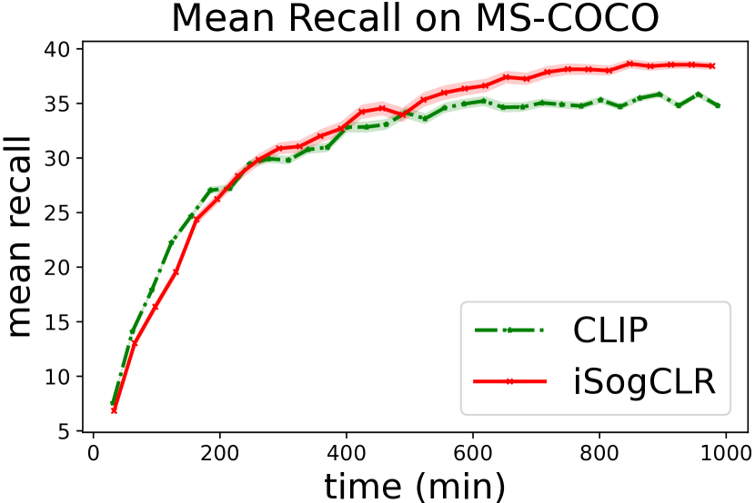
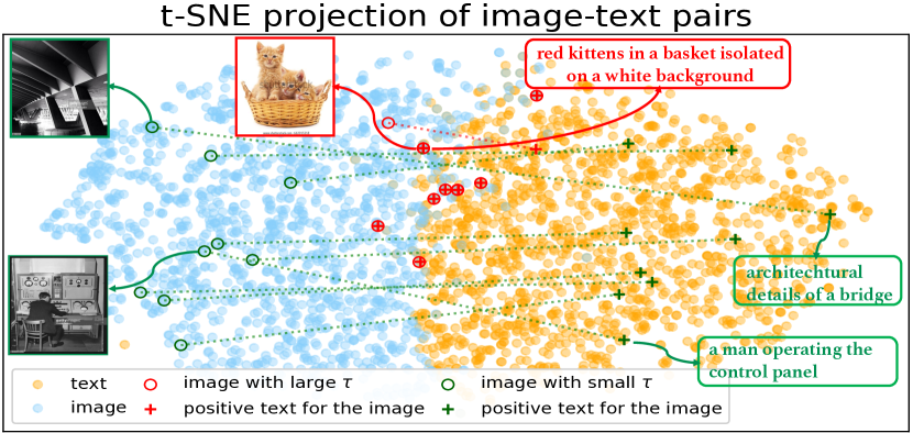
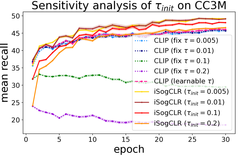
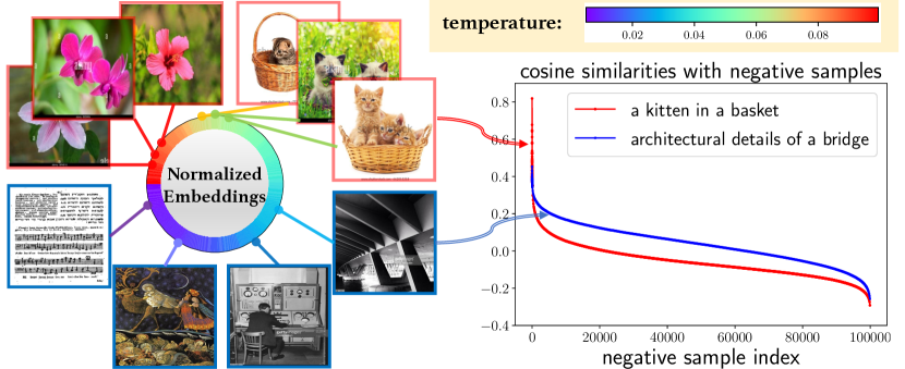
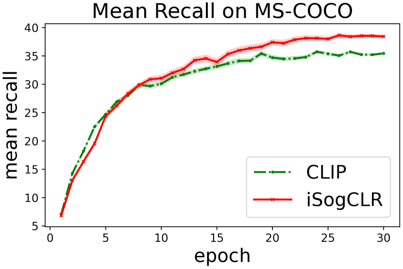
Figure 1: Left: Samples with frequent semantics (e.g., a kitten in a basket) have many more similar samples than that with rare semantics (e.g., architectural details of a bridge). Middle: An illustration of temperature individualization by our algorithm named iSogCLR, making “hot” images with frequent semantics use a higher temperature to keep semantic structures, and making “cold” images with rare semantics use a lower temperature for inducing more separable features. The circular heatmap is plotted using learned temperatures of 100 random images from the CC3M dataset. Right: Convergence curves of CLIP and iSogCLR, where we use the CLIP implementation and training settings from open-clip 222https://github.com/mlfoundations/open_clip. We train the models on CC3M and evaluate image retrieval performance on MS-COCO.

In general, contrastive methods share a common design of the softmax-based loss function, For a given anchor data i𝑖i, a contrastive loss can be written as:

coni=logexp(sim(zi,zi+)/τ)kiexp(sim(zi,zk)/τ),superscriptsubscriptcon𝑖simsubscript𝑧𝑖superscriptsubscript𝑧𝑖𝜏subscript𝑘𝑖simsubscript𝑧𝑖subscript𝑧𝑘𝜏\mathcal{L}_{\text{con}}^{i}=-\log\frac{\exp{(\text{sim}(z_{i},z_{i}^{+})}/\tau)}{\sum_{k\neq i}\exp{(\text{sim}(z_{i},z_{k})}/\tau)}, (1)

where zisubscript𝑧𝑖z_{i} is the feature of the anchor data, zi+superscriptsubscript𝑧𝑖z_{i}^{+} is the feature of a different ‘view’ of data i𝑖i and called a positive sample, zk(ki)subscript𝑧𝑘𝑘𝑖z_{k}(k\neq i) are the features of other samples and called negative samples, τ𝜏\tau is the temperature parameter, and sim(,)sim\text{sim}(\cdot,\cdot) measures the similarity between two input vectors. The positive pair can be also added to the denominator, which does not affect our discussion here. A significant property of the loss is the hardness-aware property (Wang & Liu, 2021; Zhang et al., 2022; Xia et al., 2022). Consider the gradient of τconi𝜏superscriptsubscriptcon𝑖\tau\mathcal{L}_{\text{con}}^{i} w.r.t. model parameters 𝐰𝐰\mathbf{w}, i.e., τ𝐰coni𝜏subscript𝐰superscriptsubscriptcon𝑖\tau\nabla_{\mathbf{w}}\mathcal{L}_{\text{con}}^{i}:

𝐰sim(zi,zi+)+kiexp(sim(zi,zk)/τ)kiexp(sim(zi,zk)/τ)𝐰sim(zi,zk).subscript𝐰simsubscript𝑧𝑖superscriptsubscript𝑧𝑖subscript𝑘𝑖simsubscript𝑧𝑖subscript𝑧𝑘𝜏𝑘𝑖simsubscript𝑧𝑖subscript𝑧𝑘𝜏subscript𝐰simsubscript𝑧𝑖subscript𝑧𝑘\displaystyle\small-\nabla_{\mathbf{w}}\text{sim}(z_{i},z_{i}^{+})\!+\!\sum_{k\neq i}\!\frac{\exp{(\text{sim}(z_{i},z_{k})}/\tau)}{\underset{k\neq i}{\sum}\exp{(\text{sim}(z_{i},z_{k})}/\tau)}\!\nabla_{\mathbf{w}}\text{sim}(z_{i},z_{k}).

Note that the weight for the gradient of a negative pair (zi,zk)subscript𝑧𝑖subscript𝑧𝑘(z_{i},z_{k}) is proportional to exp(sim(zi,zk)/τ)simsubscript𝑧𝑖subscript𝑧𝑘𝜏\exp{(\text{sim}(z_{i},z_{k})}/\tau). Thus, the contrastive loss automatically penalizes negative pairs according to their hardness (hard means sim(zi,zk)simsubscript𝑧𝑖subscript𝑧𝑘\text{sim}(z_{i},z_{k}) is large). The temperature τ𝜏\tau plays a critical role in controlling the penalty strength on negative samples (Wang & Liu, 2021; Zhang et al., 2022). Specifically, a small τ𝜏\tau penalizes much more on hard negative samples (i.e., the degree of hardness-awareness is high), causing separable embedding space. However, the excessive pursuit to the separability may break the underlying semantic structures because some negative samples with high similarity scores to the anchor data might indeed contain similar semantics, to which we refer as pseudo negatives. In contrast, a large τ𝜏\tau tends to treat all negative pairs equally (i.e., the degree of hardness-awareness is low) and is more tolerant to pseudo negative samples, which is beneficial for keeping local semantic structures.

Real-world data distributions always exhibit long tails (Zhu et al., 2014; Feldman, 2020) and the frequency of samples with different semantics can be extremely diverse. In Figure 2, we show some images with frequent or rare semantics from the CC3M dataset (Sharma et al., 2018). We further select two representative images, namely “a kitten in a basket” that contains frequent semantics and “architectural details of a bridge” that contains rare semantics, and present the cosine similarities between these two images and other 100,000 random texts from the same dataset. Note that images with frequent semantics have much more similar samples. To improve feature qualities, samples with frequent semantics should be assigned with a large τ𝜏\tau to better capture the local semantic structure, while using a small τ𝜏\tau will push semantically consistent samples away. On the other hand, samples with rare semantics should have a small τ𝜏\tau to make their features more discriminative and separable. We refer to these effects as semantics harmonizing. Unfortunately, most existing CL methods treat the temperature parameter as a global parameter, which does not accommodate different semantics and restricts their performance in real-world applications.

In this paper, we propose a provable stochastic algorithm for optimizing a contrastive loss with individualized temperatures. First, inspired by distributionally robust optimization (DRO) (Namkoong & Duchi, 2017; Duchi et al., 2021), we design a novel robust global contrastive loss (RGCL) for each anchor data. RGCL introduces a distributional variable for all negative samples of each anchor data (this explains “global” in RGCL), and a KL divergence constraint between the distributional variable and the uniform distribution. We show that RGCL is hardness-aware by optimizing the distributional variable, and the KL constraint affects the degree of hardness-awareness. We further demonstrate that the dual formulation of RGCL induces a loss function that can be solved efficiently and contains an individualized learnable temperature parameter. In a spirit of stochastic optimization of a global contrastive loss (SogCLR) (Yuan et al., 2022), we propose an efficient optimization algorithm named iSogCLR for solving the dual formulation of RGCL by synthesizing advanced techniques of compositional optimization (Wang & Yang, 2022) and of solving KL constrained DRO (Qi et al., 2022). We establish a convergence guarantee of our algorithm without large mini-batch sizes, which is similar to that of SogCLR for optimizing a global contrastive loss with a fixed τ𝜏\tau. Experiments on unimodal and bimodal datasets indicate that iSogCLR achieves superior performance, especially on imbalanced data. More in-depth analyses demonstrate the relationship between the semantics of data and their learned temperatures. An illustration of some images and their learned temperatures by our method is plotted in Figure 2. Besides, ablation studies show that iSogCLR is much less sensitive to its hyper-parameters. We summarize our contributions below:

  • We propose a new robust contrastive loss inspired by DRO, and study its properties and connections with existing softmax-based contrastive losses.

  • We propose a novel and provable stochastic algorithm called iSogCLR for optimizing the robust contrastive losses with automatic temperature individualization.

  • We conduct comprehensive experiments on unimodal and bimodal CL to demonstrate the superior performance of our method, and the relationship between the semantics of data and their learned temperatures.

2 Related Work

Self-supervised Learning. SSL methods can be divided into two main categories: CL methods and non-CL methods. Although non-CL methods do not rely on negative samples and achieve comparable performance to CL methods, they often require additional projector (Grill et al., 2020), stop gradient (Chen & He, 2021), or momentum encoder (Richemond et al., 2020). Several non-CL methods (Ermolov et al., 2021; Zbontar et al., 2021; Bardes et al., 2021) use information maximization techniques, which decorrelate the variables of each embedding to avoid an informational collapse. Nevertheless, CL methods remain a mainstream framework for SSL and are extended to many other fields (Khaertdinov et al., 2021; Aberdam et al., 2021; Eun et al., 2020), and are shown to be better than non-CL methods in the human learning setting (Zhuang et al., 2022).

CL Methods. Pioneering methods (Chen et al., 2020; He et al., 2020) construct pairs and optimize InfoNCE loss (Oord et al., 2018) in a direct way. Later, numerous works improve the performance by penalizing hard negatives (Wu et al., 2020; Kalantidis et al., 2020; Chen et al., 2021; Robinson et al., 2021; Xie et al., 2022; Zhang et al., 2022), generating better views (Tamkin et al., 2021; Tian et al., 2020; Ge et al., 2021; Wang & Qi, 2021), using prototypes (cluster centers) for contrasting (Caron et al., 2020; Li et al., 2020), and handling pseudo negative samples (Chuang et al., 2020; Dwibedi et al., 2021). Recently, HaoChen et al. (2021) propose a novel loss based on spectral decomposition on the population graph with accuracy guarantees. To address the issue that most CL methods rely on large batch sizes, Yuan et al. (2022) propose a provable algorithm named SogCLR for optimizing a global contrastive loss, and achieve promising results without large mini-batch sizes. Although great progress has been made, most methods ignore the imbalance of semantics in real-world data, and lack the ability to adapt to different types of semantics automatically.

Non-CL Methods. Non-CL methods employ the augmented-view-based paradigm as contrastive methods. But they only consider positive image view pairs, and use different methodologies to avoid all outputs of the network collapse to a constant. A representative class of methods aims to avoid collapse by using tricks inspired knowledge distillation (Hinton et al., 2015). Specifically, a student network is trained to predict the outputs of a teacher network, and the weights for the teacher network are updated by different strategies (Grill et al., 2020; Chen & He, 2021). An alternative class of methods (Ermolov et al., 2021; Zbontar et al., 2021; Bardes et al., 2021) relies on maximizing the information content of embeddings. They prevent informational collapse by decorrelating every pair of variables of the embedding vectors. Although these methods achieving promising results on popular tasks, theoretical studies for these methods are still lacking. Besides, it is difficulty to directly extend these methods in bimodal self-supervised learning tasks where the model architectures and data are completely different on different modalities.

Bimodal Contrastive Learning. Vision-and-language pretraining (VLP) is a rapidly growing field. Due to its effectiveness, CL has been extended to representative works such as CLIP (Radford et al., 2021) and ALIGN (Jia et al., 2021), which are pretrained on millions of web-crawled image-text pairs and achieve astounding results. Later, DeCLIP (Li et al., 2021b), FILIP (Yao et al., 2021), SLIP (Mu et al., 2022) and CyCLIP (Goel et al., 2022) improve CLIP by introducing more supervisions or bringing in fine-grained cross-modal interactions. Our algorithm tackles a fundamental problem on optimizing individualized temperatures for a contrastive loss. Thus it can be applied in bimodal setting seamlessly. Besides, because the web-crawled bimodal data often exhibits long tail distributions (Wang et al., 2022), we observe that our algorithm is more suitable in such scenario and achieves great improvements compared with baselines.

Optimizing τ𝜏\tau in CL. The impact of τ𝜏\tau on the success of CL is remarkable and noticed in prior works. Wang & Liu (2021) show that temperature controls the strength of penalties on hard negative samples and describe a uniformity-tolerance dilemma when choosing temperature parameter. Zhang et al. (2022); Khaertdinov et al. (2021) propose to improve negative mining in CL by using different temperatures for positive and negative samples, where temperatures can be fixed values or input-dependent functions.  In bimodal CL, CLIP (Radford et al., 2021) proposes to treat τ𝜏\tau as a learnable variable, which is adopted by later works (Goel et al., 2022; Li et al., 2021a). However, this approach was never rigorously justified. Zhang et al. (2021) show that input-dependent learnable τ𝜏\tau is effective to estimate the uncertainty in out-of-distribution detection, but with the cost of sacrificing the performance on downstream tasks. Different from previous methods that set or learn temperatures heuristically, we present a new view of the contrastive loss based on DRO, which explains the role of τ𝜏\tau mathematically, and enables automatic optimization of individualized temperatures.

Distributionally Robust Optimization. DRO has been extensively studied in machine learning and statistics (Bertsimas et al., 2018; Staib & Jegelka, 2019; Duchi et al., 2021). Mathematically, DRO seeks a model that performs well regardless of perturbing the sample distribution within an uncertainty set, which is specified by a divergence measure between the perturbed distribution and the observed empirical distribution (Ben-Tal et al., 2013; Blanchet et al., 2019; Duchi et al., 2021). Recent works (Qi et al., 2020, 2021, 2022; Levy et al., 2020; Jin et al., 2021; Gürbüzbalaban et al., 2022; Zhu et al., 2023) have proposed efficient stochastic algorithms for solving different DRO formulations. Our algorithm is inspired by that of Qi et al. (2022), which considers a similar DRO problem with the uncertainty set specified by a KL constraint, and proposes efficient dual-free algorithms with convergence guarantees. However, different from their work that considers an ordinary compositional objective with only one KL constraint, we deal with a more complex coupled compositional function (Wang & Yang, 2022) and many KL constraints for all anchor data, which complicate the convergence analysis.

3 Preliminaries

Let 𝒟={𝐱1,,𝐱n}𝒟subscript𝐱1subscript𝐱𝑛\mathcal{D}=\{\mathbf{x}_{1},\ldots,\mathbf{x}_{n}\} denote a set of training images with size n𝑛n. 𝒫𝒫\mathcal{P} denotes a set of data augmentation operators. Denoted by 𝒮i={𝒜(𝐱):𝒜𝒫,𝐱𝒟𝐱i}subscriptsuperscript𝒮𝑖conditional-set𝒜𝐱formulae-sequencefor-all𝒜𝒫for-all𝐱𝒟subscript𝐱𝑖\mathcal{S}^{-}_{i}=\{\mathcal{A}(\mathbf{x}):\forall\mathcal{A}\in\mathcal{P},\forall\mathbf{x}\in\mathcal{D}\setminus\mathbf{x}_{i}\} the set of negative data for the anchor image 𝐱isubscript𝐱𝑖\mathbf{x}_{i}. Let E()𝐸E(\cdot) denote the image encoder. For bimodal tasks, let 𝒟={(𝐱1,𝐭1),,(𝐱n,𝐭n)}superscript𝒟subscript𝐱1subscript𝐭1subscript𝐱𝑛subscript𝐭𝑛\mathcal{D}^{\prime}=\{(\mathbf{x}_{1},\mathbf{t}_{1}),\ldots,(\mathbf{x}_{n},\mathbf{t}_{n})\} denote n𝑛n image-text pairs. Let 𝒯i={𝐭j𝒟,ji}subscriptsuperscript𝒯𝑖formulae-sequencesubscript𝐭𝑗superscript𝒟𝑗𝑖\mathcal{T}^{-}_{i}=\{\mathbf{t}_{j}\in\mathcal{D}^{\prime},j\neq i\} be the set of negative texts for the anchor image 𝐱isubscript𝐱𝑖\mathbf{x}_{i}, and i={𝐱j𝒟,ji}subscriptsuperscript𝑖formulae-sequencesubscript𝐱𝑗superscript𝒟𝑗𝑖\mathcal{I}^{-}_{i}=\{\mathbf{x}_{j}\in\mathcal{D}^{\prime},j\neq i\} be the set of negative images for the anchor text 𝐭isubscript𝐭𝑖\mathbf{t}_{i}. Let EI()subscript𝐸𝐼E_{I}(\cdot) and ET()subscript𝐸𝑇E_{T}(\cdot) denote the encoder for images and texts in bimodal CL, respectively. Let 𝐰𝐰\mathbf{w} denote the model parameters. Denote by ΔnsubscriptΔ𝑛\Delta_{n} a simplex of dimension n𝑛n and by δΩ()subscript𝛿Ω\delta_{\Omega}(\cdot) a dirac function that returns zero if input belongs to the set ΩΩ\Omega or infinity otherwise. Let KL(,)KL\text{KL}(\cdot,\cdot) denote the KL divergence.

For unimodal CL, a global contrastive loss (GCL) (Yuan et al., 2022) for the i𝑖i-th image 𝐱isubscript𝐱𝑖\mathbf{x}_{i} can be defined as:

GCL(𝐱i)=τlogexp(E(𝒜(𝐱i))E(𝒜(𝐱i))/τ)𝐳𝒮iexp(E(𝒜(𝐱i))E(𝐳)/τ),subscriptGCLsubscript𝐱𝑖𝜏𝐸superscript𝒜subscript𝐱𝑖top𝐸superscript𝒜subscript𝐱𝑖𝜏subscript𝐳subscriptsuperscript𝒮𝑖𝐸superscript𝒜subscript𝐱𝑖top𝐸𝐳𝜏\ell_{\text{GCL}}(\mathbf{x}_{i})=-\tau\log\frac{\exp(E(\mathcal{A}(\mathbf{x}_{i}))^{\top}E(\mathcal{A}^{\prime}(\mathbf{x}_{i}))/\tau)}{\sum_{\mathbf{z}\in\mathcal{S}^{-}_{i}}\exp\left(E(\mathcal{A}(\mathbf{x}_{i}))^{\top}E(\mathbf{z})/\tau\right)}, (2)

where 𝒜,𝒜𝒫𝒜superscript𝒜𝒫\mathcal{A},\mathcal{A}^{\prime}\in\mathcal{P}. Compared with a contrastive loss defined over mini-batch samples (Chen et al., 2020; He et al., 2020), GCL multiplies τ𝜏\tau on the right side to ensure the gradient is not illy scaled. Besides, GCL considers all negative samples 𝒮isubscriptsuperscript𝒮𝑖\mathcal{S}^{-}_{i} for 𝐱isubscript𝐱𝑖\mathbf{x}_{i} in the denominator, enabling us to analyze the optimization error and design algorithms to control the error.

To simplify (2) and facilitate our statements, we define the following auxiliary function:

hi(𝐳):=E(𝒜(𝐱i))E(𝐳)E(𝒜(𝐱i))E(𝒜(𝐱i)).assignsubscript𝑖𝐳𝐸superscript𝒜subscript𝐱𝑖top𝐸𝐳𝐸superscript𝒜subscript𝐱𝑖top𝐸superscript𝒜subscript𝐱𝑖h_{i}(\mathbf{z})\!:=\!E(\mathcal{A}(\mathbf{x}_{i}))^{\top}\!E(\mathbf{z})\!-\!E(\mathcal{A}(\mathbf{x}_{i}))^{\top}\!E(\mathcal{A}^{\prime}(\mathbf{x}_{i})). (3)

In fact, hi(𝐳)subscript𝑖𝐳h_{i}(\mathbf{z}) measures the hardness score of 𝐳𝐳\mathbf{z} with respect to 𝐱isubscript𝐱𝑖\mathbf{x}_{i}. Then (2) can be rewritten as:

GCL(𝐱i)subscriptGCLsubscript𝐱𝑖\displaystyle\ell_{\text{GCL}}(\mathbf{x}_{i}) =τlog𝐳𝒮iexp(hi(𝐳)/τ).absent𝜏subscript𝐳subscriptsuperscript𝒮𝑖subscript𝑖𝐳𝜏\displaystyle=\tau\log\sum\nolimits_{\mathbf{z}\in\mathcal{S}^{-}_{i}}\exp(h_{i}(\mathbf{z})/\tau). (4)

For bimodal tasks, we consider the two-way GCL, which for the i𝑖i-th image-text pair is defined as

(𝐱i,𝐭i)=subscript𝐱𝑖subscript𝐭𝑖absent\displaystyle\ell(\mathbf{x}_{i},\mathbf{t}_{i})= τlogexp(EI(𝐱i)ET(𝐭i)/τ)𝐭𝒯iexp(EI(𝐱i)ET(𝐭)/τ)𝜏subscript𝐸𝐼superscriptsubscript𝐱𝑖topsubscript𝐸𝑇subscript𝐭𝑖𝜏subscript𝐭subscriptsuperscript𝒯𝑖subscript𝐸𝐼superscriptsubscript𝐱𝑖topsubscript𝐸𝑇𝐭𝜏\displaystyle-\tau\log\frac{\exp(E_{I}(\mathbf{x}_{i})^{\top}E_{T}(\mathbf{t}_{i})/\tau)}{\sum_{\mathbf{t}\in\mathcal{T}^{-}_{i}}\exp(E_{I}(\mathbf{x}_{i})^{\top}E_{T}(\mathbf{t})/\tau)}
τlogexp(EI(𝐱i)ET(𝐭i)/τ)𝐱iexp(EI(𝐱)ET(𝐭i)/τ),𝜏subscript𝐸𝐼superscriptsubscript𝐱𝑖topsubscript𝐸𝑇subscript𝐭𝑖𝜏subscript𝐱subscriptsuperscript𝑖subscript𝐸𝐼superscript𝐱topsubscript𝐸𝑇subscript𝐭𝑖𝜏\displaystyle-\tau\log\frac{\exp(E_{I}(\mathbf{x}_{i})^{\top}E_{T}(\mathbf{t}_{i})/\tau)}{\sum_{\mathbf{x}\in\mathcal{I}^{-}_{i}}\exp(E_{I}(\mathbf{x})^{\top}E_{T}(\mathbf{t}_{i})/\tau)},

where the first term is an image-to-text contrastive loss, i.e., try to predict 𝐭isubscript𝐭𝑖\mathbf{t}_{i} from 𝐭𝒟𝐭superscript𝒟\mathbf{t}\in\mathcal{D}^{\prime} based on 𝐱isubscript𝐱𝑖\mathbf{x}_{i}, and the second term is a symmetrical text-to-image contrastive loss.

Similar to (4), we can simplify (𝐱i,𝐭i)subscript𝐱𝑖subscript𝐭𝑖\ell(\mathbf{x}_{i},\mathbf{t}_{i}) as:

(𝐱i,𝐭i)=τlog𝐭𝒯iexp[h𝐱i(𝐭)τ]+τlog𝐱iexp[h𝐭i(𝐱)τ],subscript𝐱𝑖subscript𝐭𝑖𝜏𝐭subscriptsuperscript𝒯𝑖subscriptsubscript𝐱𝑖𝐭𝜏𝜏𝐱superscriptsubscript𝑖subscriptsubscript𝐭𝑖𝐱𝜏\small\ell(\mathbf{x}_{i},\mathbf{t}_{i})\!=\!\tau\log\!\underset{\mathbf{t}\in\mathcal{T}^{-}_{i}}{\sum}\!\exp\!\left[\!\frac{h_{\mathbf{x}_{i}}(\mathbf{t})}{\tau}\!\right]\!+\tau\!\log\!\underset{\mathbf{x}\in\mathcal{I}_{i}^{-}}{\sum}\!\exp\!\left[\!\frac{h_{\mathbf{t}_{i}}(\mathbf{x})}{\tau}\!\right],

where h𝐱i(𝐭)=EI(𝐱i)ET(𝐭)EI(𝐱i)ET(𝐭i)subscriptsubscript𝐱𝑖𝐭subscript𝐸𝐼superscriptsubscript𝐱𝑖topsubscript𝐸𝑇𝐭subscript𝐸𝐼superscriptsubscript𝐱𝑖topsubscript𝐸𝑇subscript𝐭𝑖h_{\mathbf{x}_{i}}(\mathbf{t})=E_{I}(\mathbf{x}_{i})^{\top}E_{T}(\mathbf{t})-E_{I}(\mathbf{x}_{i})^{\top}E_{T}(\mathbf{t}_{i}) and h𝐭i(𝐱)=EI(𝐱)ET(𝐭i)EI(𝐱i)ET(𝐭i)subscriptsubscript𝐭𝑖𝐱subscript𝐸𝐼superscript𝐱topsubscript𝐸𝑇subscript𝐭𝑖subscript𝐸𝐼superscriptsubscript𝐱𝑖topsubscript𝐸𝑇subscript𝐭𝑖h_{\mathbf{t}_{i}}(\mathbf{x})=E_{I}(\mathbf{x})^{\top}E_{T}(\mathbf{t}_{i})-E_{I}(\mathbf{x}_{i})^{\top}E_{T}(\mathbf{t}_{i}). Our algorithm is applicable to both unimodal and bimodal CL.

A general DRO formulation is given by (Levy et al., 2020):

min𝐰max𝐩𝒰i=1n𝐩ili(𝐰)λD(𝐩,𝟏/n),subscript𝐰subscript𝐩𝒰superscriptsubscript𝑖1𝑛subscript𝐩𝑖subscript𝑙𝑖𝐰𝜆𝐷𝐩1𝑛\min_{\mathbf{w}}\max_{\mathbf{p}\in\mathcal{U}}\sum\nolimits_{i=1}^{n}\mathbf{p}_{i}l_{i}(\mathbf{w})-\lambda D(\mathbf{p},\boldsymbol{1}/n), (5)

where 𝐩𝐩\mathbf{p} is a distributional variable, li(𝐰)subscript𝑙𝑖𝐰l_{i}(\mathbf{w}) is the loss on sample i𝑖i, 𝒰Δn𝒰subscriptΔ𝑛\mathcal{U}\subset\Delta_{n} is an uncertainty set of the distributional variable specified by some divergence constraint D(𝐩,𝟏/n)𝐷𝐩1𝑛D(\mathbf{p},\boldsymbol{1}/n). Maximizing the objective over 𝐩𝐩\mathbf{p} leads to larger weights on samples with larger losses, which actually finds the worst case loss. DRO then minimizes the worst-case loss to make models achieve the robustness against potential distribution shifts.

4 Robust Global Contrastive Objectives

We first introduce a novel robust global contrastive loss (RGCL), including its formulation and properties. Then we convert RGCL into a simpler equivalent minimization form with individualized temperatures by Lagrangian duality theory. We further give a theoretical explanation of our objective for optimizing temperatures. Due to the limited space, we describe our method in unimodal setting. For our method in bimodal setting, we present its final minimization form and defer detailed derivation to Appendix B.

4.1 Formulations

Motivated by DRO, we define the following loss for an anchor data 𝐱isubscript𝐱𝑖\mathbf{x}_{i} with a set of m𝑚m negative samples 𝒮isuperscriptsubscript𝒮𝑖\mathcal{S}_{i}^{-}:

RGCL(𝐱i):=assignsubscriptRGCLsubscript𝐱𝑖absent\displaystyle\ell_{\text{RGCL}}(\mathbf{x}_{i}):= max𝐩Δm𝐳j𝒮i𝐩jhi(𝐳j)τ0KL(𝐩,𝟏/m)subscript𝐩subscriptΔ𝑚subscriptsubscript𝐳𝑗subscriptsuperscript𝒮𝑖subscript𝐩𝑗subscript𝑖subscript𝐳𝑗subscript𝜏0KL𝐩1𝑚\displaystyle\max_{\mathbf{p}\in\Delta_{m}}\sum\nolimits_{\mathbf{z}_{j}\in\mathcal{S}^{-}_{i}}\mathbf{p}_{j}h_{i}(\mathbf{z}_{j})-\tau_{0}\text{KL}(\mathbf{p},\boldsymbol{1}/m)
s.t.KL(𝐩,𝟏/m)ρ,s.t.KL𝐩1𝑚𝜌\displaystyle\text{s.t.}\quad\text{KL}(\mathbf{p},\boldsymbol{1}/m)\leq\rho, (6)

where m=|𝒮i|𝑚superscriptsubscript𝒮𝑖m=|\mathcal{S}_{i}^{-}|, ρ>0𝜌0\rho>0 is a hyperparameter, and τ0subscript𝜏0\tau_{0} is a small positive value by default. There are several features of (6). (i) Similar to the GCL (2), we use all negative samples to define the loss. Hence our loss is referred to robust global contrastive loss. (ii) We mainly use the KL constraint KL(𝐩,𝟏/n)ρKL𝐩1𝑛𝜌\text{KL}(\mathbf{p},\boldsymbol{1}/n)\!\leq\!\rho to define an uncertainty set of 𝐩𝐩\mathbf{p}. The small KL regularization term τ0KL(𝐩,𝟏/n)subscript𝜏0KL𝐩1𝑛\tau_{0}\text{KL}(\mathbf{p},\boldsymbol{1}/n) is added to make the loss function smooth hence facilitate the optimization (Qi et al., 2022). (iii) Different from (5) that considers a distribution 𝐩𝐩\mathbf{p} over all samples, RGCL considers a distribution 𝐩𝐩\mathbf{p} over all negative samples for each anchor data.

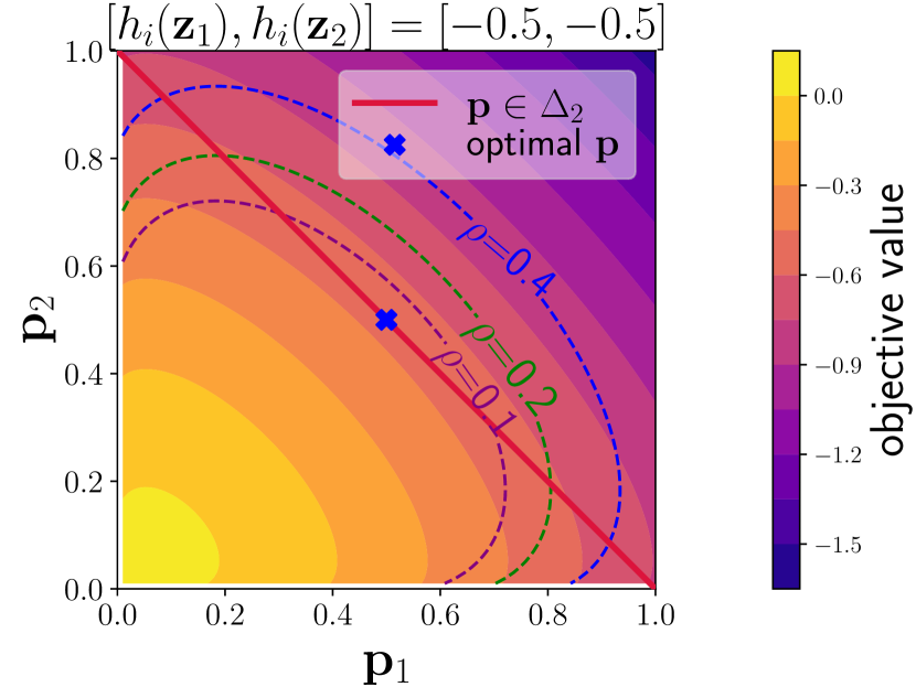
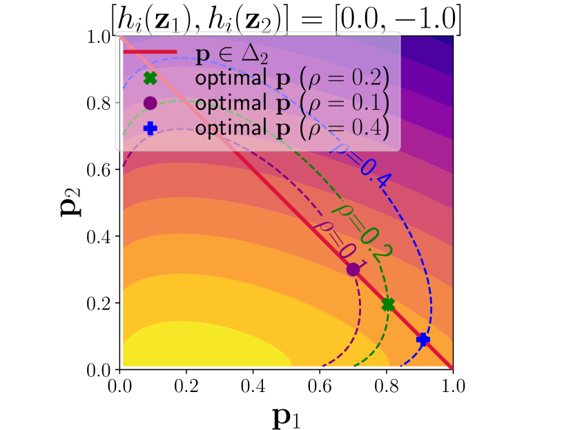
To better illustrate the key properties of RGCL, we plot the contours of RGCL(𝐱i)subscriptRGCLsubscript𝐱𝑖\ell_{\text{RGCL}}(\mathbf{x}_{i}) with two negative data in Figure 2. For [hi(𝐳1),hi(𝐳2)]subscript𝑖subscript𝐳1subscript𝑖subscript𝐳2[h_{i}(\mathbf{z}_{1}),h_{i}(\mathbf{z}_{2})] values in (6), we consider two settings, i.e., [0.0,1.0]0.01.0[0.0,-1.0] and [0.5,0.5]0.50.5[-0.5,-0.5], which represent 𝐳1subscript𝐳1\mathbf{z}_{1} is very similar to the anchor data, and two equally dissimilar negative samples, respectively. The dashed lines in Figure 2 are the boundaries of the KL constraints with different ρ𝜌\rho values, whose intersections with the red simplex lines define the feasible regions. From these figures, we observe that (i) RGCL(𝐱i)subscriptRGCLsubscript𝐱𝑖\ell_{\text{RGCL}}(\mathbf{x}_{i}) is also hardness-aware. By maximizing over 𝐩𝐩\mathbf{p}, harder negative samples will have larger weights (e.g., 𝐩=(0.8,0.2)superscript𝐩0.80.2\mathbf{p}^{*}=(0.8,0.2) for the first setting when ρ=0.2𝜌0.2\rho=0.2). (ii) If the hardness of two negative samples are similar, then their weights tend to be similar too (for the second setting). (iii) The constraint KL(𝐩,𝟏/m)ρKL𝐩1𝑚𝜌\text{KL}(\mathbf{p},\!\boldsymbol{1}/m)\!\leq\!\rho actually affects the degree of hardness-awareness. In the left of Figure 2, note that if ρ𝜌\rho gets larger, the optimal 𝐩𝐩\mathbf{p} will be more non-uniform, i.e., the degree of hardness-awareness will increase.
Refer to caption
Refer to caption
Figure 2: Contours of RGCL(𝐱i)(|𝒮i|=2)subscriptRGCLsubscript𝐱𝑖superscriptsubscript𝒮𝑖2\ell_{\text{RGCL}}(\mathbf{x}_{i})\ (|\mathcal{S}_{i}^{-}|=2) in (6) for two hi=[hi(𝐳1),hi(𝐳2)]subscript𝑖subscript𝑖subscript𝐳1subscript𝑖subscript𝐳2h_{i}=[h_{i}(\mathbf{z}_{1}),h_{i}(\mathbf{z}_{2})] vectors: [0.0,1.0]0.01.0[0.0,-1.0] and [0.5,0.5]0.50.5[-0.5,-0.5]. One can observe that RGCL(𝐱i)subscriptRGCLsubscript𝐱𝑖\ell_{\text{RGCL}}(\mathbf{x}_{i}) is hardness-aware, harder sample (hi(𝐳1)subscript𝑖subscript𝐳1h_{i}(\mathbf{z}_{1}) on the left) has larger weight (𝐩1=0.8subscript𝐩10.8\mathbf{p}_{1}=0.8). Moreover, ρ𝜌\rho affects the degree of hardness-awareness. Larger ρ𝜌\rho means higher degree of hardness-awareness.

Next, we induce an equivalent loss with an individualized learnable temperature parameter from (6) and show the intuition about the effect of τ𝜏\tau from the DRO view. Since directly optimizing (6) is challenging due to maintaining the high-dimensional distributional variable 𝐩𝐩\mathbf{p}, we follow Qi et al. (2022) and adopt the Lagrangian duality theory to convert RGCL(𝐱i)subscriptRGCLsubscript𝐱𝑖\ell_{\text{RGCL}}(\mathbf{x}_{i}) into its dual form (cf. Appendix A):

max𝐩Δmminλ0𝐳j𝒮ipjhi(𝐳j)τ0KL(𝐩,𝟏/m)λ(KL(𝐩,𝟏/m)ρ)subscript𝐩subscriptΔ𝑚subscript𝜆0subscriptsubscript𝐳𝑗subscriptsuperscript𝒮𝑖subscript𝑝𝑗subscript𝑖subscript𝐳𝑗subscript𝜏0KL𝐩1𝑚𝜆KL𝐩1𝑚𝜌\displaystyle\max_{\mathbf{p}\in\Delta_{m}}\min_{\lambda\geq 0}\!\sum_{\mathbf{z}_{j}\in\mathcal{S}^{-}_{i}}\!p_{j}h_{i}(\mathbf{z}_{j})\!-\!\tau_{0}\text{KL}(\mathbf{p},\!\boldsymbol{1}/m)\!-\!\lambda(\text{KL}(\mathbf{p},\!\boldsymbol{1}/m)\!-\!\rho)
minλ0(λ+τ0)log𝐳𝒮iexp(hi(𝐳)/λ)(λ+τ0)log(m)+λρabsentsubscript𝜆0𝜆subscript𝜏0subscript𝐳subscriptsuperscript𝒮𝑖subscript𝑖𝐳𝜆𝜆subscript𝜏0𝑚𝜆𝜌\displaystyle{\Leftrightarrow}\!\min_{\lambda\geq 0}\left(\lambda\!+\!\tau_{0}\right)\!\log\sum_{\mathbf{z}\in\mathcal{S}^{-}_{i}}\exp\!\left(h_{i}(\mathbf{z})/\lambda\right)\!-\!\left(\lambda+\tau_{0}\right)\log(m)\!+\!\lambda\rho
minττ0τlog𝔼𝐳𝒮iexp(hi(𝐳)/τ)+(ττ0)ρ,absentsubscript𝜏subscript𝜏0𝜏subscript𝔼𝐳subscriptsuperscript𝒮𝑖subscript𝑖𝐳𝜏𝜏subscript𝜏0𝜌\displaystyle\Leftrightarrow\!\min\nolimits_{\tau\geq\tau_{0}}\tau\log\mathbb{E}_{\mathbf{z}\in\mathcal{S}^{-}_{i}}\exp\!\left(h_{i}(\mathbf{z})/\tau\right)\!+\!(\tau-\tau_{0})\rho, (7)

where we first introduce a Lagrangian multiplier λ𝜆\lambda for the KL constraint, and the last equality is due to a variable change τ=λ+τ0𝜏𝜆subscript𝜏0\tau=\lambda+\tau_{0}. Notice that the Lagrangian multiplier λ𝜆\lambda for the KL constraint becomes a learnable parameter τ𝜏\tau for 𝐱isubscript𝐱𝑖\mathbf{x}_{i}. Interestingly, if we fix τ𝜏\tau (i.e., using a fixed KL regularization instead of the KL constraint in (6)), the above loss will reduce to GCL(𝐱i)subscriptGCLsubscript𝐱𝑖\ell_{\text{GCL}}\left(\mathbf{x}_{i}\right) in (2) up to a constant difference. Hence, RGCL introduces the flexibility to optimize individualized temperatures compared with the GCL.

Based on the dual form of RGCL in (7), we define a robust global contrastive objective (RGCO) for unimodal SSL :

min𝐰,𝝉τ0F(𝐰,𝝉):=1n𝐱i𝒟{𝝉ilog𝔼𝐳𝒮iexp(hi(𝐳)𝝉i)+𝝉iρ},assignsubscript𝐰𝝉subscript𝜏0𝐹𝐰𝝉1𝑛subscriptsubscript𝐱𝑖𝒟subscript𝝉𝑖subscript𝔼𝐳subscriptsuperscript𝒮𝑖subscript𝑖𝐳subscript𝝉𝑖subscript𝝉𝑖𝜌\displaystyle\small\min_{\mathbf{w},\boldsymbol{\tau}\geq\tau_{0}}\!F(\mathbf{w},\boldsymbol{\tau})\!:=\!\frac{1}{n}\!\sum_{\mathbf{x}_{i}\in\mathcal{D}}\!\left\{\!\boldsymbol{\tau}_{i}\log\!\mathop{\mathbb{E}}_{\mathbf{z}\in\mathcal{S}^{-}_{i}}\!\exp\!\left(\frac{h_{i}(\mathbf{z})}{\boldsymbol{\tau}_{i}}\right)\!+\!\boldsymbol{\tau}_{i}\rho\!\right\},

where 𝝉isubscript𝝉𝑖\boldsymbol{\tau}_{i} is the individualized temperature for 𝐱isubscript𝐱𝑖\mathbf{x}_{i}. The RGCO for bimodal SSL is defined similarly:

min𝐰,𝝉,𝝉τ0FB(𝐰,𝝉,𝝉):=1n(𝐱i,𝐭i)𝒟[(𝝉i+𝝉i)ρ+\displaystyle\min_{\mathbf{w},\boldsymbol{\tau},\boldsymbol{\tau}^{\prime}\geq\tau_{0}}\!F_{\text{B}}(\mathbf{w},\boldsymbol{\tau},\boldsymbol{\tau}^{\prime})\!:=\!\frac{1}{n}\sum\nolimits_{(\mathbf{x}_{i},\mathbf{t}_{i})\in\mathcal{D}^{\prime}}\Bigg{[}(\boldsymbol{\tau}_{i}+\boldsymbol{\tau}^{\prime}_{i})\rho+
𝝉ilog𝔼𝐭𝒯iexp(h𝐱i(𝐭)𝝉i)+𝝉ilog𝔼𝐱iexp(h𝐭i(𝐱)𝝉i)],\displaystyle\boldsymbol{\tau}_{i}\log{\mathbb{E}}_{\mathbf{t}\in\mathcal{T}_{i}^{-}}\exp\!\left(\frac{h_{\mathbf{x}_{i}}(\mathbf{t})}{\boldsymbol{\tau}_{i}}\right)\!+\!\boldsymbol{\tau}^{\prime}_{i}\log{\mathbb{E}}_{\mathbf{x}\in\mathcal{I}^{-}_{i}}\!\exp\!\left(\frac{h_{\mathbf{t}_{i}}(\mathbf{x})}{\boldsymbol{\tau}^{\prime}_{i}}\!\right)\!\Bigg{]},

with individualized temperatures 𝝉isubscript𝝉𝑖\boldsymbol{\tau}_{i} and 𝝉isuperscriptsubscript𝝉𝑖\boldsymbol{\tau}_{i}^{\prime} for images and texts, respectively. A small constant can be added inside the log to ensure its smoothness and Lipschitz continuity as in (Yuan et al., 2022), which is assumed for analysis.

4.2 An Intuitive Theoretical Explanation

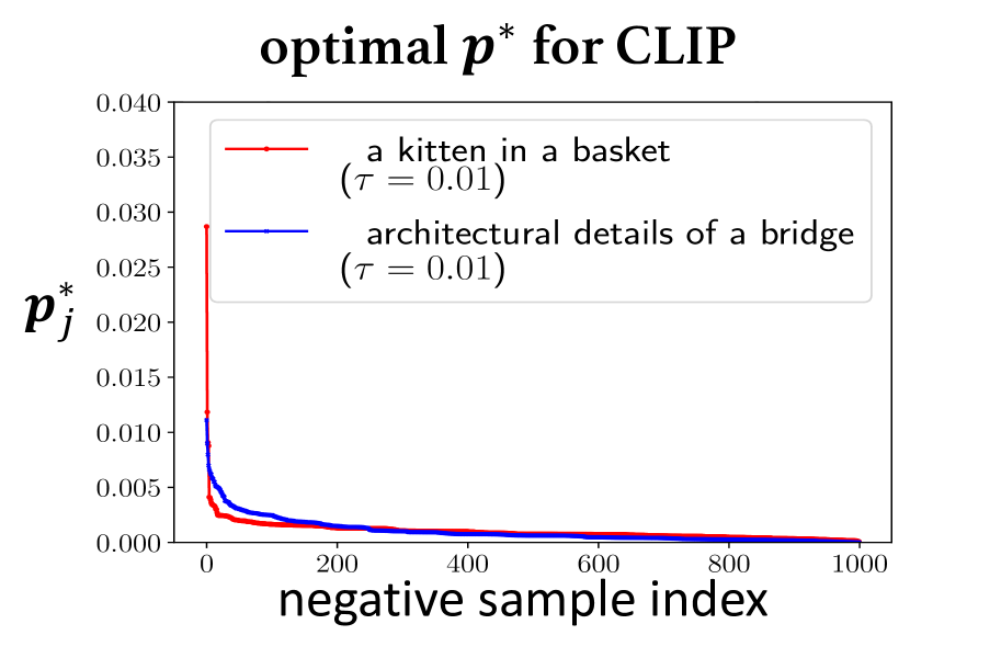
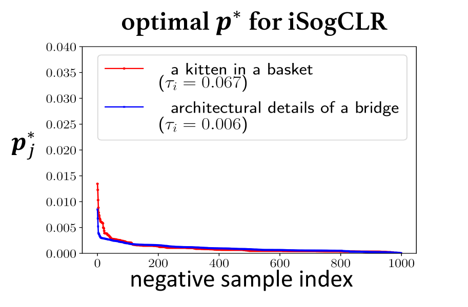
To answer why our RGCL can learn suitable temperatures for samples with different semantics intuitively, we compare our iSogCLR (the algorithm for optimizing RCGL) with CLIP, whose learned global τ𝜏\tau is 0.01 on CC3M. Considering the representative cat and bridge images, we extract the features of them and 1000 random samples as their negatives for each method. Then we substitute these features into (6) and solve the optimal 𝐩superscript𝐩\mathbf{p}^{*} (i.e., 𝐩j=exp(hi(𝐳j)/τ)𝐳𝒮iexp(hi(𝐳j)/τ)subscriptsuperscript𝐩𝑗subscript𝑖subscript𝐳𝑗𝜏subscript𝐳superscriptsubscript𝒮𝑖subscript𝑖subscript𝐳𝑗𝜏\mathbf{p}^{*}_{j}=\frac{\exp(h_{i}(\mathbf{z}_{j})/\tau)}{\sum_{\mathbf{z}\in\mathcal{S}_{i}^{-}}\exp(h_{i}(\mathbf{z}_{j})/\tau)}, cf. Appendix A) of each image for both methods. We plot the results in Figure 3. Combining these results with the formulation (7), we have the following explanation.
Refer to caption
Refer to caption
Figure 3: For the anchor images of cat and bridge, we select 1000 negative samples and solve (6) for the optimal 𝐩superscript𝐩\mathbf{p}^{*} by using hisubscript𝑖h_{i} values of iSogCLR with learned 𝝉isubscript𝝉𝑖\boldsymbol{\tau}_{i} and CLIP with learned τ𝜏\tau.

For samples with frequent semantics, due to the hardness-aware property of RGCL, their optimal 𝐩superscript𝐩\mathbf{p}^{*} in (6) tend to be more non-uniform, and KL(𝐩,𝟏/n)ρKL𝐩1𝑛𝜌\text{KL}(\mathbf{p},\boldsymbol{1}/n)\leq\rho is more likely to be violated. Therefore, their Lagrangian multipliers λ𝜆\lambda in (7) will be large to “push” 𝐩𝐩\mathbf{p} back to be closer to uniform. Due to τ=λ+τ0𝜏𝜆subscript𝜏0\tau=\lambda+\tau_{0}, their temperatures will be large. From Figure 3, it is notable that compared with the optimal 𝐩superscript𝐩\mathbf{p}^{*} of the cat image from CLIP (the red line in the right), that from our RGCL (the red line in the left) is more uniform.

For samples with rare semantics, their optimal distributional variables 𝐩𝐩\mathbf{p} in (6) tend to be more uniform, which makes KL(𝐩,𝟏/n)ρKL𝐩1𝑛𝜌\text{KL}(\mathbf{p},\boldsymbol{1}/n)\leq\rho being more likely to be satisfied. At this time, their Lagrangian multipliers λ𝜆\lambda are probably small, and thus their temperatures are small. For example, the learned τ𝜏\tau of the bridge image by iSogCLR is 0.006, which is smaller than the final learned τ=0.01𝜏0.01\tau\!=\!0.01 in CLIP.

5 iSogCLR for Stochastic Optimization

In this section, we design a provable algorithm for optimizing F(𝐰,𝝉)𝐹𝐰𝝉F(\mathbf{w},\boldsymbol{\tau}). The algorithm for FB(𝐰,𝝉,𝝉)subscript𝐹B𝐰𝝉superscript𝝉F_{\text{B}}(\mathbf{w},\boldsymbol{\tau},\boldsymbol{\tau}^{\prime}) is similar and deferred to Appendix B. The new objective functions F(𝐰,𝝉)𝐹𝐰𝝉F(\mathbf{w},\boldsymbol{\tau}) and FB(𝐰,𝝉,𝝉)subscript𝐹B𝐰𝝉superscript𝝉F_{\text{B}}(\mathbf{w},\boldsymbol{\tau},\boldsymbol{\tau}^{\prime}) are special cases of X-risks (Yang, 2022), making the optimization of them much more challenging than traditional empirical risk minimization. Nonetheless, existing algorithms for deep X-risk optimization are not directly applicable due to the optimization over many temperature variables.

Inspired by Yuan et al. (2022) for solving GCL, we cast F(𝐰,𝝉)𝐹𝐰𝝉F(\mathbf{w},\boldsymbol{\tau}) as a finite-sum coupled compositional optimization problem (Wang & Yang, 2022):

min𝐰,𝝉ΩF(𝐰,𝝉):=1n𝐱i𝒟fi(𝝉i,gi(𝐰,𝝉i;𝒮i))Fi(𝐰,𝝉i),assignsubscript𝐰𝝉Ω𝐹𝐰𝝉1𝑛subscriptsimilar-tosubscript𝐱𝑖𝒟subscriptsubscript𝑓𝑖subscript𝝉𝑖subscript𝑔𝑖𝐰subscript𝝉𝑖subscriptsuperscript𝒮𝑖subscript𝐹𝑖𝐰subscript𝝉𝑖\displaystyle\min_{\mathbf{w},\boldsymbol{\tau}\in\Omega}F(\mathbf{w},\boldsymbol{\tau}):=\frac{1}{n}\sum_{\mathbf{x}_{i}\sim\mathcal{D}}\underbrace{f_{i}\left(\boldsymbol{\tau}_{i},g_{i}(\mathbf{w},\boldsymbol{\tau}_{i};\mathcal{S}^{-}_{i})\right)}_{F_{i}(\mathbf{w},\boldsymbol{\tau}_{i})}, (8)

where 𝝉Ω𝝉Ω\boldsymbol{\tau}\in\Omega is to accommodate the constraint on 𝝉𝝉\boldsymbol{\tau} and

fi(𝝉i,)=𝝉ilog()+𝝉iρ,subscript𝑓𝑖subscript𝝉𝑖subscript𝝉𝑖subscript𝝉𝑖𝜌\displaystyle f_{i}(\boldsymbol{\tau}_{i},\cdot)=\boldsymbol{\tau}_{i}\log(\cdot)+\boldsymbol{\tau}_{i}\rho,
gi(𝐰,𝝉i;𝒮i)=𝔼𝐳𝒮iexp(hi(𝐳)/𝝉i).subscript𝑔𝑖𝐰subscript𝝉𝑖superscriptsubscript𝒮𝑖subscript𝔼𝐳subscriptsuperscript𝒮𝑖subscript𝑖𝐳subscript𝝉𝑖\displaystyle g_{i}(\mathbf{w},\boldsymbol{\tau}_{i};\mathcal{S}_{i}^{-})=\mathbb{E}_{\mathbf{z}\in\mathcal{S}^{-}_{i}}\exp\left(h_{i}(\mathbf{z})/{\boldsymbol{\tau}_{i}}\right).

The gradients of F𝐹F w.r.t. 𝐰𝐰\mathbf{w} and 𝝉isubscript𝝉𝑖\boldsymbol{\tau}_{i} can be computed by:

𝐰F(𝐰,𝝉)=1n𝐱i𝒟𝐰Fi(𝐰,𝝉i)subscript𝐰𝐹𝐰𝝉1𝑛subscriptsubscript𝐱𝑖𝒟subscript𝐰subscript𝐹𝑖𝐰subscript𝝉𝑖\displaystyle\nabla_{\mathbf{w}}F(\mathbf{w},\boldsymbol{\tau})=\frac{1}{n}\sum_{\mathbf{x}_{i}\in\mathcal{D}}\nabla_{\mathbf{w}}F_{i}(\mathbf{w},\boldsymbol{\tau}_{i}) (9)
=1n𝐱i𝒟gifi(𝝉i,gi(𝐰,𝝉i;𝒮i))𝐰gi(𝐰,𝝉i;𝒮i),absent1𝑛subscriptsubscript𝐱𝑖𝒟subscriptsubscript𝑔𝑖subscript𝑓𝑖subscript𝝉𝑖subscript𝑔𝑖𝐰subscript𝝉𝑖superscriptsubscript𝒮𝑖subscript𝐰subscript𝑔𝑖𝐰subscript𝝉𝑖superscriptsubscript𝒮𝑖\displaystyle=\frac{1}{n}\sum_{\mathbf{x}_{i}\in\mathcal{D}}\nabla_{g_{i}}f_{i}(\boldsymbol{\tau}_{i},g_{i}(\mathbf{w},\boldsymbol{\tau}_{i};\mathcal{S}_{i}^{-}))\nabla_{\mathbf{w}}g_{i}(\mathbf{w},\boldsymbol{\tau}_{i};\mathcal{S}_{i}^{-}),
𝝉iF(𝐰,𝝉)=1n𝐱j𝒟𝝉iFj(𝐰,𝝉j)=(a)1n𝝉iFi(𝐰,𝝉i)subscriptsubscript𝝉𝑖𝐹𝐰𝝉1𝑛subscriptsubscript𝐱𝑗𝒟subscriptsubscript𝝉𝑖subscript𝐹𝑗𝐰subscript𝝉𝑗superscript𝑎1𝑛subscriptsubscript𝝉𝑖subscript𝐹𝑖𝐰subscript𝝉𝑖\displaystyle\nabla_{\boldsymbol{\tau}_{i}}\!F(\mathbf{w},\boldsymbol{\tau})\!=\!\frac{1}{n}\!\sum_{\mathbf{x}_{j}\in\mathcal{D}}\!\nabla_{\boldsymbol{\tau}_{i}}\!F_{j}(\mathbf{w},\boldsymbol{\tau}_{j})\!\stackrel{{\scriptstyle(a)}}{{=}}\!\frac{1}{n}\!\nabla_{\boldsymbol{\tau}_{i}}\!F_{i}(\mathbf{w},\boldsymbol{\tau}_{i}) (10)
=1n(𝝉i𝝉igi(𝐰,𝝉i;𝒮i)gi(𝐰,𝝉i;𝒮i)+log(gi(𝐰,𝝉i;𝒮i))+ρ),absent1𝑛subscript𝝉𝑖subscriptsubscript𝝉𝑖subscript𝑔𝑖𝐰subscript𝝉𝑖superscriptsubscript𝒮𝑖subscript𝑔𝑖𝐰subscript𝝉𝑖superscriptsubscript𝒮𝑖subscript𝑔𝑖𝐰subscript𝝉𝑖superscriptsubscript𝒮𝑖𝜌\displaystyle=\frac{1}{n}\bigg{(}\frac{\boldsymbol{\tau}_{i}\nabla_{\boldsymbol{\tau}_{i}}g_{i}(\mathbf{w},\boldsymbol{\tau}_{i};\mathcal{S}_{i}^{-})}{g_{i}(\mathbf{w},\boldsymbol{\tau}_{i};\mathcal{S}_{i}^{-})}+\log(g_{i}(\mathbf{w},\boldsymbol{\tau}_{i};\mathcal{S}_{i}^{-}))+\rho\bigg{)},

where (a)𝑎(a) holds because for ji𝑗𝑖j\neq i, Fj(𝐰,𝝉j)subscript𝐹𝑗𝐰subscript𝝉𝑗F_{j}(\mathbf{w},\boldsymbol{\tau}_{j}) does not involve 𝝉isubscript𝝉𝑖\boldsymbol{\tau}_{i}. Note that the major cost for computing (9) and (10) lies at computing gi(𝐰,𝝉i;𝒮i)subscript𝑔𝑖𝐰subscript𝝉𝑖superscriptsubscript𝒮𝑖g_{i}(\mathbf{w},\boldsymbol{\tau}_{i};\mathcal{S}_{i}^{-}) and its gradients w.r.t. 𝐰𝐰\mathbf{w} and 𝝉isubscript𝝉𝑖\boldsymbol{\tau}_{i}, involving all samples in 𝒮isuperscriptsubscript𝒮𝑖\mathcal{S}_{i}^{-}. At each iteration, we only sample a random mini-batch of B𝐵B samples ={𝐱1,𝐱2,,𝐱B}subscript𝐱1subscript𝐱2subscript𝐱𝐵\mathcal{B}=\{\mathbf{x}_{1},\mathbf{x}_{2},\ldots,\mathbf{x}_{B}\}, and compute an unbiased estimator of gi(𝐰,𝝉i;𝒮i)subscript𝑔𝑖𝐰subscript𝝉𝑖superscriptsubscript𝒮𝑖g_{i}(\mathbf{w},\boldsymbol{\tau}_{i};\mathcal{S}_{i}^{-}) for each 𝐱isubscript𝐱𝑖\mathbf{x}_{i}\in\mathcal{B} by:

gi(𝐰,𝝉i;i)=1|i|𝐳iexp(hi(𝐳)/𝝉i),subscript𝑔𝑖𝐰subscript𝝉𝑖subscript𝑖1subscript𝑖subscript𝐳subscript𝑖subscript𝑖𝐳subscript𝝉𝑖g_{i}(\mathbf{w},\boldsymbol{\tau}_{i};\mathcal{B}_{i})=\frac{1}{|\mathcal{B}_{i}|}\!\sum\nolimits_{\mathbf{z}\in\mathcal{B}_{i}}\exp(h_{i}(\mathbf{z})/\boldsymbol{\tau}_{i}), (11)

where i={𝒜(𝐱),𝒜(𝐱):𝒜,𝒜𝒫,𝐱𝐱i}subscript𝑖conditional-set𝒜𝐱superscript𝒜𝐱formulae-sequence𝒜superscript𝒜𝒫𝐱subscript𝐱𝑖\mathcal{B}_{i}\!=\!\left\{\mathcal{A}(\mathbf{x}),\mathcal{A}^{\prime}(\mathbf{x})\!:\!\mathcal{A},\mathcal{A}^{\prime}\!\in\!\mathcal{P},\mathbf{x}\!\in\!\mathcal{B}\!\setminus\!\mathbf{x}_{i}\right\} contains the negative samples of 𝐱isubscript𝐱𝑖\mathbf{x}_{i} in \mathcal{B}. However, directly substituting gi(𝐰,𝝉i;i)subscript𝑔𝑖𝐰subscript𝝉𝑖subscript𝑖g_{i}(\mathbf{w},\boldsymbol{\tau}_{i};\mathcal{B}_{i}) as the estimator of gi(𝐰,𝝉i;𝒮i)subscript𝑔𝑖𝐰subscript𝝉𝑖superscriptsubscript𝒮𝑖g_{i}(\mathbf{w},\boldsymbol{\tau}_{i};\mathcal{S}_{i}^{-}) into (9) and (10) will yield biased estimators because (9) and (10) are non-linear w.r.t. gi(𝐰,𝝉i;𝒮i)subscript𝑔𝑖𝐰subscript𝝉𝑖superscriptsubscript𝒮𝑖g_{i}(\mathbf{w},\boldsymbol{\tau}_{i};\mathcal{S}_{i}^{-}). The optimization error will be large when the batch size is small (Yuan et al., 2022).

To control the approximation error and provide a convergence guarantee, we borrow a technique from Yuan et al. (2022) by using a moving average estimator to keep track of gi(𝐰,𝝉i;𝒮i)subscript𝑔𝑖𝐰subscript𝝉𝑖superscriptsubscript𝒮𝑖g_{i}(\mathbf{w},\boldsymbol{\tau}_{i};\mathcal{S}_{i}^{-}) for each 𝐱i𝒟subscript𝐱𝑖𝒟\mathbf{x}_{i}\in\mathcal{D}. To this end, we maintain a scalar 𝐬isubscript𝐬𝑖\mathbf{s}_{i} for each 𝐱isubscript𝐱𝑖\mathbf{x}_{i} and update it at the t𝑡t-th iteration by:

𝐬it+1=(1β0)𝐬it+β0gi(𝐰t,𝝉it;i),superscriptsubscript𝐬𝑖𝑡11subscript𝛽0superscriptsubscript𝐬𝑖𝑡subscript𝛽0subscript𝑔𝑖subscript𝐰𝑡superscriptsubscript𝝉𝑖𝑡subscript𝑖\mathbf{s}_{i}^{t+1}=(1-\beta_{0})\mathbf{s}_{i}^{t}+\beta_{0}g_{i}(\mathbf{w}_{t},\boldsymbol{\tau}_{i}^{t};\mathcal{B}_{i}), (12)

where β0(0,1)subscript𝛽001\beta_{0}\in(0,1). Intuitively, when t𝑡t increases, 𝐰t1subscript𝐰𝑡1\mathbf{w}_{t-1} and 𝝉t1superscript𝝉𝑡1\boldsymbol{\tau}^{t-1} are getting close to 𝐰tsubscript𝐰𝑡\mathbf{w}_{t} and 𝝉tsuperscript𝝉𝑡\boldsymbol{\tau}^{t}, hence the previous value of 𝐬itsuperscriptsubscript𝐬𝑖𝑡\mathbf{s}_{i}^{t} is useful for estimating gisubscript𝑔𝑖g_{i}. With these stochastic estimators, we compute the gradients of (8) in terms of 𝐰tsubscript𝐰𝑡\mathbf{w}_{t} and 𝝉itsuperscriptsubscript𝝉𝑖𝑡\boldsymbol{\tau}_{i}^{t} with controllable approximation error by:

G(𝝉it)=1n[𝝉it𝐬it𝝉igi(𝐰,𝝉i;i)+log(𝐬it)+ρ],𝐺superscriptsubscript𝝉𝑖𝑡1𝑛delimited-[]superscriptsubscript𝝉𝑖𝑡superscriptsubscript𝐬𝑖𝑡subscriptsubscript𝝉𝑖subscript𝑔𝑖𝐰subscript𝝉𝑖subscript𝑖superscriptsubscript𝐬𝑖𝑡𝜌\displaystyle G(\boldsymbol{\tau}_{i}^{t})=\frac{1}{n}\left[\frac{\boldsymbol{\tau}_{i}^{t}}{\mathbf{s}_{i}^{t}}\nabla_{\boldsymbol{\tau}_{i}}g_{i}(\mathbf{w},\boldsymbol{\tau}_{i};\mathcal{B}_{i})+\log(\mathbf{s}_{i}^{t})+\rho\right], (13)
G(𝐰t)=1B𝐱i𝝉it𝐬it𝐰gi(𝐰,𝝉i;i).𝐺subscript𝐰𝑡1𝐵subscriptsubscript𝐱𝑖superscriptsubscript𝝉𝑖𝑡superscriptsubscript𝐬𝑖𝑡subscript𝐰subscript𝑔𝑖𝐰subscript𝝉𝑖subscript𝑖\displaystyle G(\mathbf{w}_{t})=\frac{1}{B}\sum_{\mathbf{x}_{i}\in\mathcal{B}}\frac{\boldsymbol{\tau}_{i}^{t}}{\mathbf{s}_{i}^{t}}\nabla_{\mathbf{w}}g_{i}(\mathbf{w},\boldsymbol{\tau}_{i};\mathcal{B}_{i}). (14)

The complete procedure is presented in Algorithm 1, named iSogCLR with i standing for individualization of temperatures. In step 1, we initialize all 𝝉isubscript𝝉𝑖\boldsymbol{\tau}_{i} to τinitsubscript𝜏init\tau_{\text{init}}. We implement the momentum update for 𝝉it+1superscriptsubscript𝝉𝑖𝑡1\boldsymbol{\tau}_{i}^{t+1} and 𝐰t+1subscript𝐰𝑡1\mathbf{w}_{t+1} in Step 8, 9 and Step 12, 13, respectively, where β1(0,1)subscript𝛽101\beta_{1}\in(0,1) is the momentum parameter. The momentum-style update can be replaced by an Adam-style update using adaptive step sizes and the same convergence rate can be established (Guo et al., 2021).

In terms of the additional memory cost, while it scales with the number of samples, it typically is not a significant concern in practical applications. Firstly, the additional memory cost is still small compared with the number of model parameters. For example, the additional memory cost for 1 million samples is 2×106×410242=7.632superscript1064superscript102427.632\times\frac{10^{6}\times 4}{1024^{2}}=7.63MB. Secondly, the GPU memory usage can be optimized by storing variables 𝐬isubscript𝐬𝑖\mathbf{s}_{i}, 𝐮isubscript𝐮𝑖\mathbf{u}_{i} and 𝝉isubscript𝝉𝑖\boldsymbol{\tau}_{i} in the CPU memory. To further minimize the impact on training time, one can employ an asynchronous strategy to transfer data. Specifically, before the t𝑡t-th iteration, we can prefetch 𝐬itsuperscriptsubscript𝐬𝑖𝑡\mathbf{s}_{i}^{t}, 𝐮itsuperscriptsubscript𝐮𝑖𝑡\mathbf{u}_{i}^{t} and 𝝉itsuperscriptsubscript𝝉𝑖𝑡\boldsymbol{\tau}_{i}^{t} from the CPU and transfer them to the GPU. After forward propagation, we conduct back-propagation and asynchronously copy the updated 𝐬it+1superscriptsubscript𝐬𝑖𝑡1\mathbf{s}_{i}^{t+1}, 𝐮it+1superscriptsubscript𝐮𝑖𝑡1\mathbf{u}_{i}^{t+1} and 𝝉it+1superscriptsubscript𝝉𝑖𝑡1\boldsymbol{\tau}_{i}^{t+1} back to the CPU memory and fetch a new batch of them from CPU. By utilizing high-bandwidth CPU-GPU interconnects, such as PCIe4 or NVLink, the time required to transfer these variables can effectively overlap with the time of back-propagation. This approach facilitates fast training and reduces GPU memory consumption.

Algorithm 1 iSogCLR
0:  β0,β1,ηsubscript𝛽0subscript𝛽1𝜂\beta_{0},\beta_{1},\eta
1:  Initialize 𝐰1,𝐬1,𝐮1,𝐯1subscript𝐰1superscript𝐬1superscript𝐮1subscript𝐯1\mathbf{w}_{1},\mathbf{s}^{1},\mathbf{u}^{1},\mathbf{v}_{1}, 𝝉1=𝝉initsuperscript𝝉1subscript𝝉init\boldsymbol{\tau}^{1}=\boldsymbol{\tau_{\text{init}}}
2:  for t=1,2,,T𝑡12𝑇t=1,2,\dots,T do
3:     Draw a batch of B𝐵B samples denoted by 𝒟𝒟\mathcal{B}\subset\mathcal{D}
4:     for 𝐱isubscript𝐱𝑖\mathbf{x}_{i}\in\mathcal{B} do
5:        Compute gi(𝐰t,𝝉it;i)subscript𝑔𝑖subscript𝐰𝑡superscriptsubscript𝝉𝑖𝑡subscript𝑖g_{i}(\mathbf{w}_{t},\boldsymbol{\tau}_{i}^{t};\mathcal{B}_{i}) according to (11)
6:        Update 𝐬it+1superscriptsubscript𝐬𝑖𝑡1\mathbf{s}_{i}^{t+1} according to (12)
7:        Compute G(𝝉it)𝐺superscriptsubscript𝝉𝑖𝑡G(\boldsymbol{\tau}_{i}^{t}) according to (13)
8:        Update 𝐮it+1=(1β1)𝐮it+β1G(𝝉it)superscriptsubscript𝐮𝑖𝑡11subscript𝛽1superscriptsubscript𝐮𝑖𝑡subscript𝛽1𝐺superscriptsubscript𝝉𝑖𝑡\mathbf{u}_{i}^{t+1}=(1-\beta_{1})\mathbf{u}_{i}^{t}+\beta_{1}G(\boldsymbol{\tau}_{i}^{t})
9:        Update 𝝉it+1=ΠΩ[𝝉itη𝐮it+1]superscriptsubscript𝝉𝑖𝑡1subscriptΠΩdelimited-[]superscriptsubscript𝝉𝑖𝑡𝜂superscriptsubscript𝐮𝑖𝑡1\boldsymbol{\tau}_{i}^{t+1}=\Pi_{\Omega}\left[\boldsymbol{\tau}_{i}^{t}-\eta\mathbf{u}_{i}^{t+1}\right]
10:     end for
11:     Compute gradient estimator G(𝐰t)𝐺subscript𝐰𝑡G(\mathbf{w}_{t}) according to (14)
12:     Compute 𝐯t+1=(1β1)𝐯t+β1G(𝐰t)subscript𝐯𝑡11subscript𝛽1subscript𝐯𝑡subscript𝛽1𝐺subscript𝐰𝑡\mathbf{v}_{t+1}=(1-\beta_{1})\mathbf{v}_{t}+\beta_{1}G(\mathbf{w}_{t})
13:     Update 𝐰t+1=𝐰tη𝐯t+1subscript𝐰𝑡1subscript𝐰𝑡𝜂subscript𝐯𝑡1\mathbf{w}_{t+1}=\mathbf{w}_{t}-\eta\mathbf{v}_{t+1} (or Adam-style)
14:  end for

We highlight the differences between RGCO/iSogCLR and GCO/SogCLR (Yuan et al., 2022) and our contributions of analysis: (i) RGCO has additional n𝑛n temperature variables 𝝉isubscript𝝉𝑖\boldsymbol{\tau}_{i}; nevertheless we prove the same iteration complexity as SogCLR. (ii) the constraint 𝝉iτ0subscript𝝉𝑖subscript𝜏0\boldsymbol{\tau}_{i}\geq\tau_{0} makes the analysis more complicated. In particular, to show F(𝐰,𝝉)𝐹𝐰𝝉F(\mathbf{w},\boldsymbol{\tau}) is smooth in terms of (𝐰,𝝉)𝐰𝝉(\mathbf{w},\boldsymbol{\tau}), we follow Qi et al. (2022) to derive an upper bound τmaxsubscript𝜏\tau_{\max} for the optimal 𝝉subscript𝝉\boldsymbol{\tau}_{*} and use the constraint set Ω={τ0ττmax}Ωsubscript𝜏0𝜏subscript𝜏\Omega=\{\tau_{0}\leq\bf\tau\leq\tau_{\max}\} in the analysis. (iii) Due to the constraint on 𝝉𝝉\boldsymbol{\tau}, we employ a different notion of stationary point using the regular subgradient (cf. Appendix D) of the non-smooth extended objective F¯(𝐰,𝝉)=F(𝐰,𝝉)+δΩ(𝝉)¯𝐹𝐰𝝉𝐹𝐰𝝉subscript𝛿Ω𝝉\bar{F}(\mathbf{w},\boldsymbol{\tau})=F(\mathbf{w},\boldsymbol{\tau})+\delta_{\Omega}(\boldsymbol{\tau}), i.e., ^F¯(𝐰,𝝉)^¯𝐹𝐰𝝉\hat{\partial}\bar{F}(\mathbf{w},\boldsymbol{\tau}), which also complicates the analysis. Finally, the convergence guarantee of iSogCLR is:

Theorem 1.

Under appropriate conditions and settings of parameters β0,β1=𝒪(Bϵ2)subscript𝛽0subscript𝛽1𝒪superscript𝐵superscriptitalic-ϵ2\beta_{0},\beta_{1}\!=\!\mathcal{O}(B^{\prime}\epsilon^{2}), η=𝒪(BBϵ2n)𝜂𝒪𝐵superscript𝐵superscriptitalic-ϵ2𝑛\eta\!=\!\mathcal{O}\!\left(\!\frac{BB^{\prime}\epsilon^{2}}{n}\!\right), where B=||,B=|i|formulae-sequence𝐵superscript𝐵subscript𝑖B\!=\!|\mathcal{B}|,B^{\prime}\!=\!|\mathcal{B}_{i}|, after T=𝒪(nBBϵ4)𝑇𝒪𝑛𝐵superscript𝐵superscriptitalic-ϵ4T\!=\!\mathcal{O}\!\left(\!\frac{n}{BB^{\prime}\epsilon^{4}}\!\right) iterations Algorithm 1 finds an ϵitalic-ϵ\epsilon-stationary solution of the problem, i.e., 𝔼[dist(0,^F¯(𝐰t,𝛕t))2]ϵ2𝔼delimited-[]distsuperscript0^¯𝐹subscript𝐰𝑡subscript𝛕𝑡2superscriptitalic-ϵ2\mathbb{E}[\text{dist}(0,\hat{\partial}\bar{F}(\mathbf{w}_{t},\boldsymbol{\tau}_{t}))^{2}]\!\leq\!\epsilon^{2} for a random t{1,,T}𝑡1𝑇t\in\{1,\ldots,T\}.

Remark: The theorem indicates that iSogCLR has the same 𝒪(1ϵ4)𝒪1superscriptitalic-ϵ4\mathcal{O}\left(\frac{1}{\epsilon^{4}}\right) complexity as SogCLR (Yuan et al., 2022). We refer the interested readers to Appendix D for the proof, where we also exhibit the conditions similar to (Yuan et al., 2022).

6 Experiments

Table 1: Linear evaluation results with 400 pretraining epochs on six unimodal image datasets. We report the average top-1 accuracies (%) and standard deviation over 3 runs with different random seeds. Full results are provided in Table 3 and 4 in Appendix C.3.
Method CIFAR10 CIFAR100 ImageNet100 CIFAR10-LT CIFAR100-LT iNaturalist
SimCLR 88.74±plus-or-minus\pm0.18 62.34±plus-or-minus\pm0.09 79.96±plus-or-minus\pm0.20 77.09±plus-or-minus\pm0.13 49.33±plus-or-minus\pm0.12 91.52±plus-or-minus\pm0.17
Barlow Twins 87.39±plus-or-minus\pm0.14 62.28±plus-or-minus\pm0.13 79.16±plus-or-minus\pm0.13 75.94±plus-or-minus\pm0.08 48.39±plus-or-minus\pm0.14 91.89±plus-or-minus\pm0.21
FlatCLR 88.61±plus-or-minus\pm0.10 63.27±plus-or-minus\pm0.07 80.24±plus-or-minus\pm0.16 77.96±plus-or-minus\pm0.12 52.61±plus-or-minus\pm0.06 92.54±plus-or-minus\pm0.09
Spectral CL 88.77±plus-or-minus\pm0.09 63.06±plus-or-minus\pm0.18 80.48±plus-or-minus\pm0.08 76.38±plus-or-minus\pm0.21 51.86±plus-or-minus\pm0.16 92.13±plus-or-minus\pm0.16
SogCLR 88.93±plus-or-minus\pm0.11 63.14±plus-or-minus\pm0.12 80.54±plus-or-minus\pm0.14 77.70±plus-or-minus\pm0.07 52.35±plus-or-minus\pm0.08 92.60±plus-or-minus\pm0.08
VICReg 88.96±plus-or-minus\pm0.16 62.44±plus-or-minus\pm0.13 80.16±plus-or-minus\pm0.22 75.05±plus-or-minus\pm0.09 48.43±plus-or-minus\pm0.13 93.03±plus-or-minus\pm0.14
SimCo 88.86±plus-or-minus\pm0.12 62.67±plus-or-minus\pm0.06 79.73±plus-or-minus\pm0.17 77.71±plus-or-minus\pm0.13 51.06±plus-or-minus\pm0.09 92.10±plus-or-minus\pm0.12
iSogCLR 89.24±plus-or-minus\pm0.15 63.82±plus-or-minus\pm0.14 81.14±plus-or-minus\pm0.19 78.37±plus-or-minus\pm0.16 53.06±plus-or-minus\pm0.12 93.08±plus-or-minus\pm0.19

In this section, we conduct experiments on unimodal and bimodal datasets and observe that our algorithm outperforms prior strong baselines. Moreover, in-depth analyses show that the samples with different semantics are indeed assigned with suitable temperatures. We also perform ablation studies to better understand the behaviors of iSogCLR. The code to reproduce the results in this paper is available at https://github.com/zhqiu/contrastive-learning-iSogCLR/.

In unimodal setting, We compare our iSogCLR with five CL methods: SimCLR (Chen et al., 2020), FlatCLR (Chen et al., 2021), SimCo (Zhang et al., 2022), Spectral CL (HaoChen et al., 2021), SogCLR (Yuan et al., 2022), and two non-contrastive methods: Barlow Twins (Zbontar et al., 2021) and VICReg (Bardes et al., 2021). In bimodal setting, we compare with CLIP (Radford et al., 2021), CyCLIP (Goel et al., 2022), and SogCLR.

For fair comparison, we set the hyper-parameters of all methods using grid search. SimCLR, FlatCLR, and SogCLR contain τ𝜏\tau, which is tuned in a range of {0.1,0.3,0.5,0.7}0.10.30.50.7\{0.1,0.3,0.5,0.7\}. For other methods, we fine-tune their hyper-parameters around the recommended values in their papers. Following Radford et al. (2021); Goel et al. (2022), τ𝜏\tau is directly optimized in CLIP and CyCLIP. The detailed implementation and data information are in Appendix C.1 and C.2, respectively.

Table 2: Results on two bimodal downstream tasks. For image-text retrieval on Flickr30K and MSCOCO, we compute IR@111 and TR@111 for the Recall@111 on image-retrieval (IR) and text-retrieval (TR). For classification tasks, we compute top-111 accuracy (%). We report the average of scores and standard deviation over 3 runs with different random seeds. Full results are in Table 56, and 7 in Appendix C.3.

Method Flickr30K Retrieval MSCOCO Retrieval Zero-shot Classification top-1 Acc
IR@1 TR@1 IR@1 TR@1 CIFAR10 CIFAR100 ImageNet1K
CLIP 40.98±plus-or-minus\pm0.22 50.90±plus-or-minus\pm0.17 21.32±plus-or-minus\pm0.12 26.98±plus-or-minus\pm0.21 60.63±plus-or-minus\pm0.19 30.70±plus-or-minus\pm0.11 36.27±plus-or-minus\pm0.17
CyCLIP 42.46±plus-or-minus\pm0.13 51.70±plus-or-minus\pm0.23 21.58±plus-or-minus\pm0.19 26.18±plus-or-minus\pm0.24 57.19±plus-or-minus\pm0.20 33.11±plus-or-minus\pm0.14 36.75±plus-or-minus\pm0.21
SogCLR 43.32±plus-or-minus\pm0.18 57.18±plus-or-minus\pm0.20 22.43±plus-or-minus\pm0.13 30.08±plus-or-minus\pm0.22 61.09±plus-or-minus\pm0.24 33.26±plus-or-minus\pm0.12 37.46±plus-or-minus\pm0.19
iSogCLR 44.36±plus-or-minus\pm0.12 60.20±plus-or-minus\pm0.26 23.27±plus-or-minus\pm0.18 32.72±plus-or-minus\pm0.13 58.91±plus-or-minus\pm0.15 33.81±plus-or-minus\pm0.18 40.72±plus-or-minus\pm0.23

6.1 Unimodal Experiments

Data. We consider three balanced datasets: CIFAR10, CIFAR100, ImageNet100 (Wu et al., 2019), and three imbalanced datasets: CIFAR10-LT, CIFAR100-LT, iNaturalist2018 (Horn et al., 2018). ImageNet100 is a subset with 100 classes from ImageNet1K (Russakovsky et al., 2015). CIFAR10-LT and CIFAR100-LT are created following the Long-Tailed (LT) imbalance setting (Cui et al., 2019) and widely used (Cao et al., 2019; Cui et al., 2019; Qi et al., 2020). The iNaturalist dataset is a large-scale dataset with dramatically different number of images per category. We use its official training and validation splits.

Setup. The backbone network, initial learning rate and batch size are set to ResNet-18, 0.8, and 128 for CIFAR datasets. While for ImageNet100 and iNaturalist2018, they are set to ResNet-50, 1.2, and 256, respectively. The projection head has three linear layers, each with 8192 output units. The first two layers of the projector are followed by a BN layer and rectified linear units. We employ LARS optimizer (You et al., 2017) (with a momentum of 0.9 and weight decay of 1e-4) and cosine learning rate schedule. We also use learning rate warm-up for 10 epochs, i.e., learning rate is gradually increased to the maximum value. We resize input images to 224×\times224 and follow the same image augmentation strategies as in SimCLR (Chen et al., 2020) including random crop, color distortion, and Gaussian blur. For linear evaluation, we train the last classification layer using SGD with Nesterov momentum with a batch size of 256 for 100 epochs. The initial learning rate is set to 30.0 and decayed by 0.2 at 40, 60, and 80 epochs. We tune β0subscript𝛽0\beta_{0} and ρ𝜌\rho in our algorithm from {0.7,0.8,0.9}0.70.80.9\{0.7,0.8,0.9\} and {0.1,0.2,0.3,0.4}0.10.20.30.4\{0.1,0.2,0.3,0.4\}, respectively. τinitsubscript𝜏init\tau_{\text{init}} and τ0subscript𝜏0\tau_{0} are set to 0.7 and 0.05 by default.

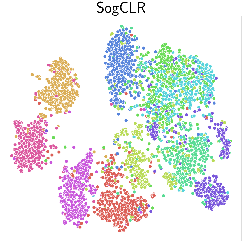
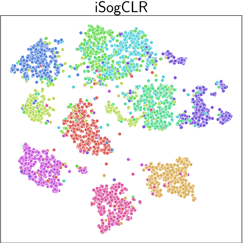
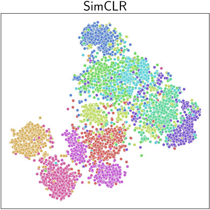
Results. We present partial results in Table 1 and full results in Table 34 in Appendix C.3. First, comparing iSogCLR, SogCLR and SimCLR, we observe that (i) SogCLR is generally better than SimCLR, showing the advantage of optimizing a GCL under limited mini-batch sizes; and (ii) iSogCLR outperforms SogCLR in all cases, confirming the effectiveness of individualized temperatures. In Figure 5, we visualize the learned embeddings from these three methods on CIFAR10, where each color represents a class. Note that the class boundaries of iSogCLR are more clear than that of others, indicating that iSogCLR indeed improves feature qualities. We also observe that iSogCLR outperforms prior strong baselines, e.g., VICReg, Spectral CL. Besides, iSogCLR achieves larger improvements on imbalanced data, e.g., has relative improvements of 2.37% and 7.56% over SimCLR on CIFAR100 and CIFAR100-LT, respectively.

6.2 Bimodal Experiments

Data. We adopt Conceptual Captions 3M (CC3M) (Sharma et al., 2018) dataset, which is widely used in vision-and-language pretraining (Li et al., 2021b; Mu et al., 2022; Goel et al., 2022). Because some links of the images in CC3M have expired, the number of pairs we downloaded is about 2.85M, which is smaller than 3.3M in original paper. During evaluation, we use two common bimodal datasets: Flickr30K (Plummer et al., 2015), MSCOCO (Lin et al., 2014), obtained from the well-known Karpathy split (Karpathy & Fei-Fei, 2015), and three standard image datasets: CIFAR10, CIFAR100, and ImageNet1K.

Setup. Following recent studies on bimodal SSL (Li et al., 2021a; Dou et al., 2022), we adopt ResNet-50 and DistilBert (Sanh et al., 2019) as the image and text encoder, which are initialized with weights from unimodal pretraining. Specifically, we use the ResNet-50 model pretrained on ImageNet from timm library (Wightman, 2019). The DistilBert model comes from huggingface library (Wolf et al., 2020), which is pretrained on BookCorpus (Zhu et al., 2015) and English Wikipedia. The output embedding of each encoder is then transformed to a lower-dimensional (256-d) representation by a linear layer and normalized for computing contrastive loss. We use a batch size of 512 for 30 epochs pre-training, where the image resolution is 256×\times256. We employ Adam-W optimizer (Loshchilov & Hutter, 2017) with cosine learning rate decay. The learning rate is warmed-up to 2e-4 in the first 1000 iterations and decayed to 1e-6 by a cosine decay scheduler. We employ Adam-W optimizer (Loshchilov & Hutter, 2017) with the weight decay of 0.02. We tune β0subscript𝛽0\beta_{0} and ρ𝜌\rho from {0.7,0.8,0.9}0.70.80.9\{0.7,0.8,0.9\} and {5.8,6.0,6.2,6.4}5.86.06.26.4\{5.8,6.0,6.2,6.4\}, respectively. τinitsubscript𝜏init\tau_{\text{init}} and τ0subscript𝜏0\tau_{0} are set to 0.01 and 0.005 by default. We evaluate models on two downstream tasks: cross-modal retrieval and image classification in zero-shot setting, following the widely-used evaluation protocol (Radford et al., 2021; Goel et al., 2022).
Refer to caption
Refer to caption
Refer to caption
Figure 4: The arrangement of features (projected using t-SNE) for CIFAR10 samples learned by SimCLR, SogCLR and iSogCLR.
Refer to caption
Refer to caption
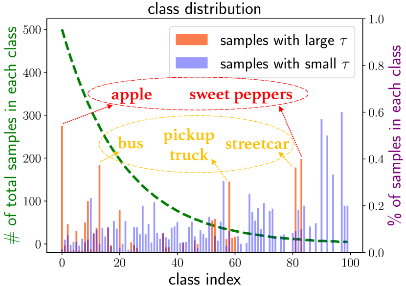
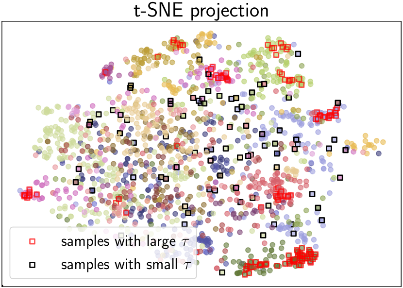
Figure 5: The class distributions and t-SNE projection for samples with large and small τ𝜏\tau values in CIFAR100-LT. Left: The green dashed line and left axis denote the number of samples in each class, the red/blue bars and right axis denote the proportions of samples with large/small τ𝜏\tau values in each class. Right: Each color represents a superclass in CIFAR100-LT.
Refer to caption
Refer to caption
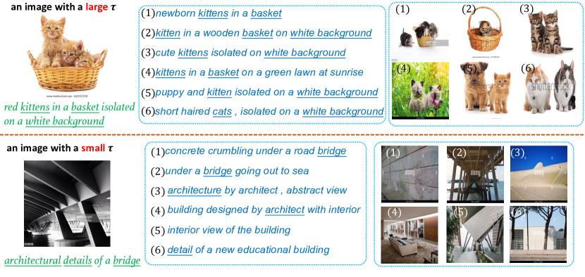
Figure 6: In-depth analyses on CC3M. Left: the contents of several hard negative image-text pairs of the cat and bridge images. Right: the tSNE of learned representations of sampled image-text pairs, with large and small temperatures marked by red and green, respectively.
Refer to caption
Refer to caption
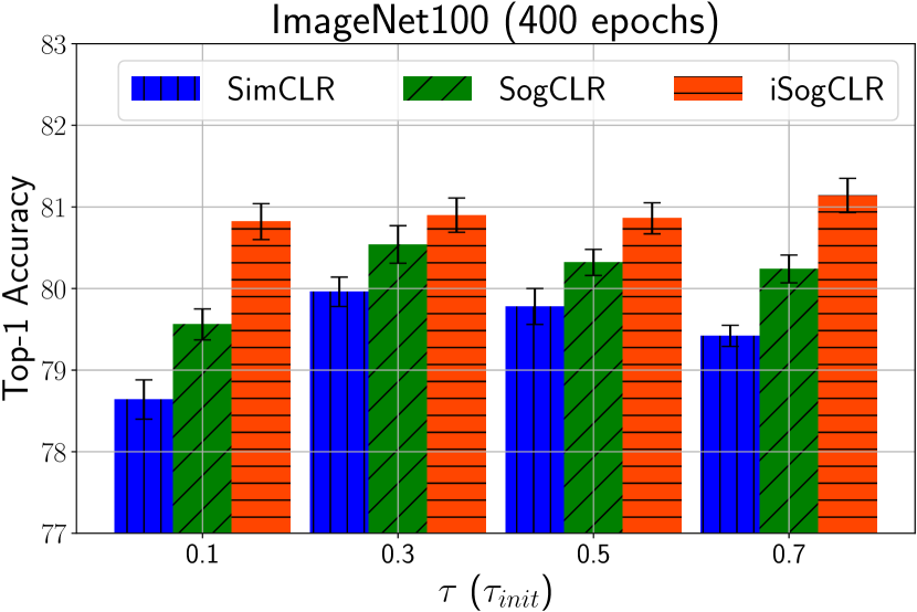
Figure 7: Effect of τ𝜏\tau and τinitsubscript𝜏init\tau_{\text{init}} on SimCLR/SogCLR and iSogCLR.

Results. We present partial results in Table 2 and full results in Table 567 in Appendix C.3. Compared with baselines, our algorithm achieves significant improvements on both downstream tasks. Specifically, iSogCLR improves CLIP by 4%similar-to\sim17% and 2%similar-to\sim8% on image-text retrieval and zero-short classification, respectively. Large-scale bimodal data always contain long-tail underlying semantics (Wang et al., 2022), thus the optimal τ𝜏\tau of different samples may vary greatly. Hence iSogCLR with individualized temperatures is much more suitable than the methods with a global τ𝜏\tau.

6.3 In-depth Analyses

Here, we demonstrate that iSogCLR indeed assigns suitable temperatures to samples with different types of semantics. Specifically, we consider the following two scenarios.

Unimodal data. We use CIFAR100-LT to study the characteristics of samples with different τ𝜏\tau values. First, we select top-600 samples with large temperatures and bottom-600 samples with small temperatures. The class distributions of these two groups of samples are in the left of Figure 5. We observe that samples with small τ𝜏\tau account for a higher proportion of tail classes. Interestingly, although some of samples belong to tail classes, e.g., ‘sweet peppers’, ‘streetcar’ and ‘pickup truck’, they are semantically similar to some head classes, e.g., ‘apple’, ‘bus’. Thus these samples actually have frequent semantics and iSogCLR correctly assigns them large τ𝜏\tau values. The right part of Figure 5 shows the projection of samples in these two groups. Note that most of samples with large τ𝜏\tau values are in the centers of clusters, while most of samples with small τ𝜏\tau values are separated from clusters. These results clearly show that iSogCLR makes samples with frequent semantics have large τ𝜏\tau values to keep semantic structures, and makes samples with rare semantics have small τ𝜏\tau values to be more discriminative.

Bimodal data. First, we use the data of “a kitten in a basket” and “architectural details of a bridge” for more illustrations. We show several hard negative pairs of the cat and bridge images in the left of Figure 6. One can observe that for the cat image, its hard negative pairs contain very similar semantics. For the bridge image, however, it has fewer hard negative pairs with similar semantics with it. We also present learned features of 1500 random image-text pairs with highlights on several pairs with large and small τ𝜏\tau values in Figure 6 (right). Notice that images with large τ𝜏\tau values are very close to their texts, while images with small τ𝜏\tau values are far from their texts. The reason is that pairs with large τ𝜏\tau values have frequent semantics, thus the model learns their patterns well and their features are well aligned. By contrast, the pairs with small τ𝜏\tau values have rare semantics and their features are not learned so well. These results show that iSogCLR learns suitable temperatures for samples with different semantics. More samples in CC3M data are provided in Figure 10 and 11 in Appendix C.3, showing that images with large τ𝜏\tau values are related to frequent human activities or life scenes, while images with small τ𝜏\tau values correspond to rare activities or scenes.

Refer to caption
Refer to caption
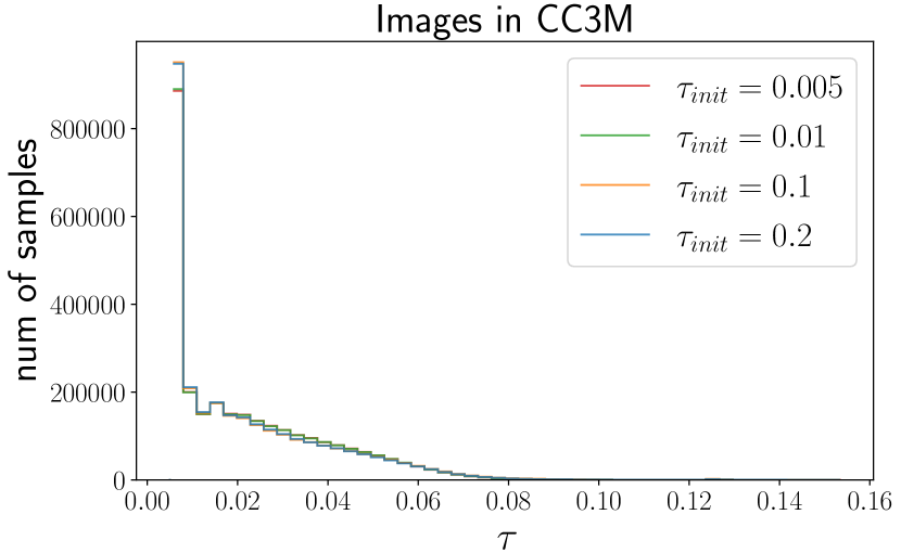
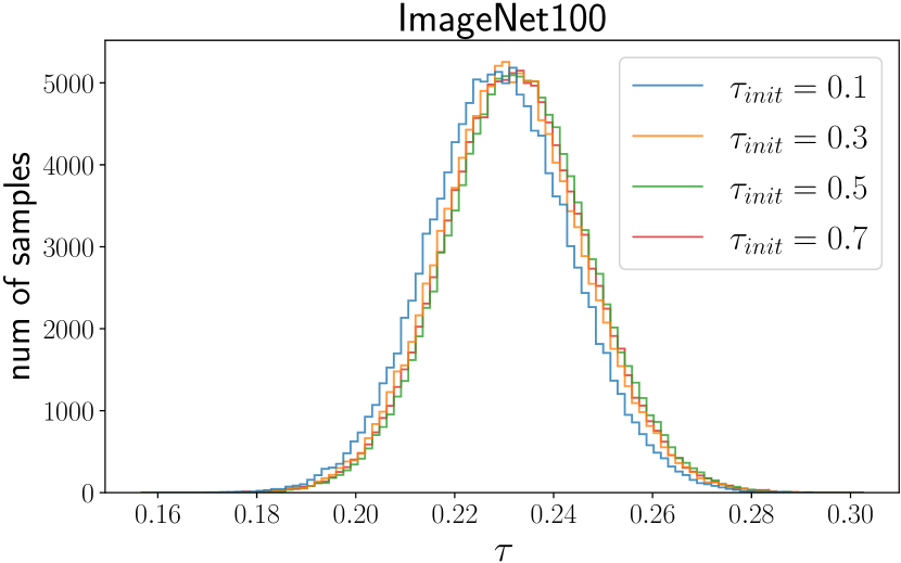
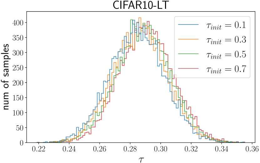
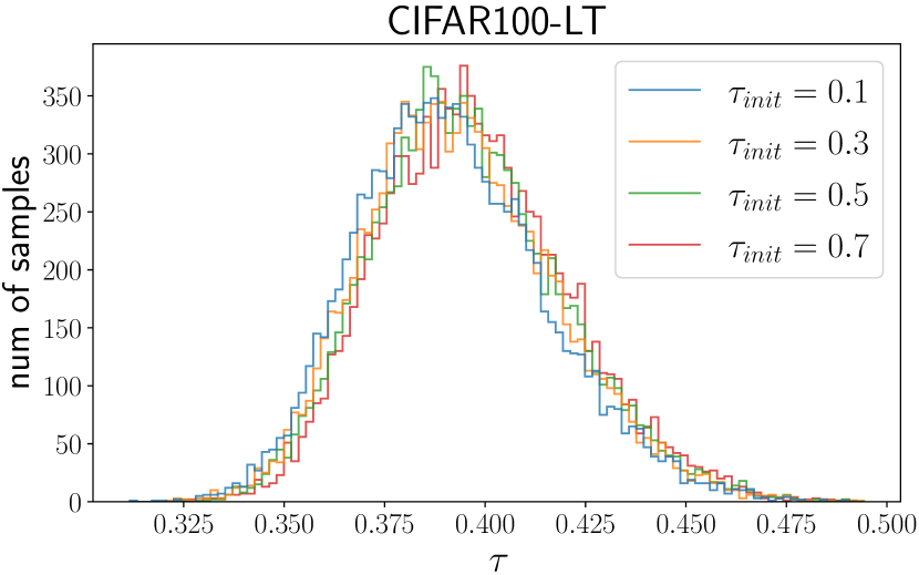
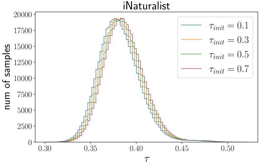
Figure 8: Final distributions of learned temperatures.

6.4 Ablation Studies

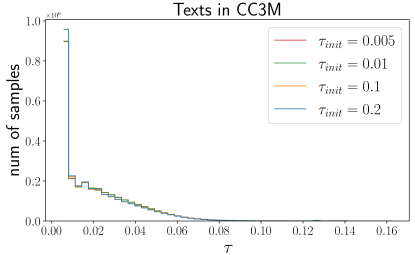
In this section, we conduct extensive ablation studies to shed light on the behaviors of iSogCLR. First, we study the effect of different τinitsubscript𝜏init\tau_{\text{init}} values on the final performance and convergence of iSogCLR, and provide the results in Figure 7. From the left part of Figure 7, one can observe that iSogCLR is not sensitive to τinitsubscript𝜏init\tau_{\text{init}} and always outperforms SimCLR/SogCLR with a tuned τ𝜏\tau. More results are in Table 8 in Appendix C.3. The results on CC3M in the right of Figure 7 indicate that CLIP fails to converge when τ𝜏\tau is fixed to a large value (e.g., 0.1, 0.2). On the contrary, regardless of the values of τinitsubscript𝜏init\tau_{\text{init}}, iSogCLR converges well and matches or outperforms CLIP with the tuned or learned τ𝜏\tau.

We further visualize the final distributions of learned temperatures on different datasets in Figure 8. Note that these distributions are similar regardless of τinitsubscript𝜏init\tau_{\text{init}} values. We also observe that the distributions on unimodal data usually follow a Gaussian distribution, while that on bimodal CC3M data has a long-tail (cf. Figure 9 in Appendix C.3 for more results). It is interesting to observe that the learned temperatures for bimodal dataset are smaller than those for image datasets, which is consistent with the literature found by manual tuning (Chen et al., 2020; Liang et al., 2022).

Due to the limited space, more studies are provided in Appendix C.3. In particular, the results about the effect of hyper-parameter ρ𝜌\rho in Table 9 indicate that iSogCLR is not sensitive to ρ𝜌\rho. We also compare with other heuristic baselines with individualized learnable temperatures in Appendix C.3, and show that our method is more advantageous for learning individualized temperatures (cf. Table 10).

7 Conclusion

In this work, we propose a novel method named iSogCLR for contrastive SSL with automatic temperature individualization. We first design a novel robust global contrastive objective based on DRO. Then we propose a provable stochastic algorithm. Theoretical and experimental results show that iSogCLR finds suitable temperatures for different samples. Comprehensive experiments demonstrate the effectiveness of iSogCLR on both unimodal and bimodal tasks.

References

  • Aberdam et al. (2021) Aberdam, A., Litman, R., Tsiper, S., Anschel, O., Slossberg, R., Mazor, S., Manmatha, R., and Perona, P. Sequence-to-sequence contrastive learning for text recognition. In Proceedings of the 34th IEEE/CVF Conference on Computer Vision and Pattern Recognition, pp.  15302–15312, 2021.
  • Bardes et al. (2021) Bardes, A., Ponce, J., and LeCun, Y. Vicreg: Variance-invariance-covariance regularization for self-supervised learning. arXiv preprint arXiv:2105.04906, 2021.
  • Ben-Tal et al. (2013) Ben-Tal, A., Den Hertog, D., De Waegenaere, A., Melenberg, B., and Rennen, G. Robust solutions of optimization problems affected by uncertain probabilities. Management Science, 59(2):341–357, 2013.
  • Bertsimas et al. (2018) Bertsimas, D., Gupta, V., and Kallus, N. Data-driven robust optimization. Mathematical Programming, 167(2):235–292, 2018.
  • Blanchet et al. (2019) Blanchet, J., Kang, Y., and Murthy, K. Robust wasserstein profile inference and applications to machine learning. Journal of Applied Probability, 56(3):830–857, 2019.
  • Cao et al. (2019) Cao, K., Wei, C., Gaidon, A., Arechiga, N., and Ma, T. Learning imbalanced datasets with label-distribution-aware margin loss. In Advances in Neural Information Processing Systems, volume 32, pp.  1565–1576, 2019.
  • Caron et al. (2020) Caron, M., Misra, I., Mairal, J., Goyal, P., Bojanowski, P., and Joulin, A. Unsupervised learning of visual features by contrasting cluster assignments. In Advances in Neural Information Processing Systems, volume 33, pp.  9912–9924, 2020.
  • Chen et al. (2021) Chen, J., Gan, Z., Li, X., Guo, Q., Chen, L., Gao, S., Chung, T., Xu, Y., Zeng, B., Lu, W., et al. Simpler, faster, stronger: Breaking the log-k curse on contrastive learners with flatnce. arXiv preprint arXiv:2107.01152, 2021.
  • Chen et al. (2020) Chen, T., Kornblith, S., Norouzi, M., and Hinton, G. A simple framework for contrastive learning of visual representations. In Proceedings of the 37th International Conference on Machine Learning, pp.  1597–1607, 2020.
  • Chen & He (2021) Chen, X. and He, K. Exploring simple siamese representation learning. In Proceedings of the 34th IEEE/CVF Conference on Computer Vision and Pattern Recognition, pp.  15750–15758, 2021.
  • Chuang et al. (2020) Chuang, C.-Y., Robinson, J., Lin, Y.-C., Torralba, A., and Jegelka, S. Debiased contrastive learning. In Advances in Neural Information Processing Systems, volume 33, pp.  8765–8775, 2020.
  • Cui et al. (2019) Cui, Y., Jia, M., Lin, T.-Y., Song, Y., and Belongie, S. Class-balanced loss based on effective number of samples. In Proceedings of the 32rd IEEE/CVF conference on computer vision and pattern recognition, pp.  9268–9277, 2019.
  • Dou et al. (2022) Dou, Z.-Y., Kamath, A., Gan, Z., Zhang, P., Wang, J., Li, L., Liu, Z., Liu, C., LeCun, Y., Peng, N., et al. Coarse-to-fine vision-language pre-training with fusion in the backbone. In Advances in Neural Information Processing Systems, volume 35, pp.  9694–9705, 2022.
  • Duchi et al. (2021) Duchi, J. C., Glynn, P. W., and Namkoong, H. Statistics of robust optimization: A generalized empirical likelihood approach. Mathematics of Operations Research, 46(3):946–969, 2021.
  • Dwibedi et al. (2021) Dwibedi, D., Aytar, Y., Tompson, J., Sermanet, P., and Zisserman, A. With a little help from my friends: Nearest-neighbor contrastive learning of visual representations. In Proceedings of the 34th IEEE/CVF International Conference on Computer Vision, pp.  9588–9597, 2021.
  • Ermolov et al. (2021) Ermolov, A., Siarohin, A., Sangineto, E., and Sebe, N. Whitening for self-supervised representation learning. In Proceedings of the 38th International Conference on Machine Learning, pp.  3015–3024, 2021.
  • Eun et al. (2020) Eun, H., Moon, J., Park, J., Jung, C., and Kim, C. Learning to discriminate information for online action detection. In Proceedings of the 33rd IEEE/CVF Conference on Computer Vision and Pattern Recognition, pp.  809–818, 2020.
  • Feldman (2020) Feldman, V. Does learning require memorization? a short tale about a long tail. In Proceedings of the 52nd Annual ACM SIGACT Symposium on Theory of Computing, pp.  954–959, 2020.
  • Ge et al. (2021) Ge, S., Mishra, S., Li, C.-L., Wang, H., and Jacobs, D. Robust contrastive learning using negative samples with diminished semantics. In Advances in Neural Information Processing Systems, volume 34, pp.  27356–27368, 2021.
  • Goel et al. (2022) Goel, S., Bansal, H., Bhatia, S., Rossi, R. A., Vinay, V., and Grover, A. Cyclip: Cyclic contrastive language-image pretraining. arXiv preprint arXiv:2205.14459, 2022.
  • Goyal et al. (2021) Goyal, P., Caron, M., Lefaudeux, B., Xu, M., Wang, P., Pai, V., Singh, M., Liptchinsky, V., Misra, I., Joulin, A., et al. Self-supervised pretraining of visual features in the wild. arXiv preprint arXiv:2103.01988, 2021.
  • Grill et al. (2020) Grill, J.-B., Strub, F., Altché, F., Tallec, C., Richemond, P., Buchatskaya, E., Doersch, C., Avila Pires, B., Guo, Z., Gheshlaghi Azar, M., et al. Bootstrap your own latent-a new approach to self-supervised learning. In Advances in Neural Information Processing Systems, volume 33, pp.  21271–21284, 2020.
  • Guo et al. (2021) Guo, Z., Xu, Y., Yin, W., Jin, R., and Yang, T. On stochastic moving-average estimators for non-convex optimization. arXiv preprint arXiv:2104.14840, 2021.
  • Gürbüzbalaban et al. (2022) Gürbüzbalaban, M., Ruszczyński, A., and Zhu, L. A stochastic subgradient method for distributionally robust non-convex and non-smooth learning. Journal of Optimization Theory and Applications, 194(3):1014–1041, 2022.
  • HaoChen et al. (2021) HaoChen, J. Z., Wei, C., Gaidon, A., and Ma, T. Provable guarantees for self-supervised deep learning with spectral contrastive loss. In Advances in Neural Information Processing Systems, volume 34, pp.  5000–5011, 2021.
  • He et al. (2020) He, K., Fan, H., Wu, Y., Xie, S., and Girshick, R. Momentum contrast for unsupervised visual representation learning. In Proceedings of the 33rd IEEE/CVF Conference on Computer Vision and Pattern Recognition, pp.  9729–9738, 2020.
  • Hinton et al. (2015) Hinton, G., Vinyals, O., Dean, J., et al. Distilling the knowledge in a neural network. arXiv preprint arXiv:1503.02531, 2(7), 2015.
  • Horn et al. (2018) Horn, G. V., Aodha, O. M., Song, Y., Cui, Y., Sun, C., Shepard, A., Adam, H., Perona, P., and Belongie, S. J. The inaturalist species classification and detection dataset. In Proceedings of the 31st IEEE/CVF Conference on Computer Vision and Pattern Recognition, pp.  8769–8778, 2018.
  • Huang et al. (2022) Huang, Z., Jin, X., Lu, C., Hou, Q., Cheng, M.-M., Fu, D., Shen, X., and Feng, J. Contrastive masked autoencoders are stronger vision learners. arXiv preprint arXiv:2207.13532, 2022.
  • Jia et al. (2021) Jia, C., Yang, Y., Xia, Y., Chen, Y.-T., Parekh, Z., Pham, H., Le, Q., Sung, Y.-H., Li, Z., and Duerig, T. Scaling up visual and vision-language representation learning with noisy text supervision. In Proceedings of the 38th International Conference on Machine Learning, pp.  4904–4916, 2021.
  • Jin et al. (2021) Jin, J., Zhang, B., Wang, H., and Wang, L. Non-convex distributionally robust optimization: Non-asymptotic analysis. In Advances in Neural Information Processing Systems, volume 34, pp.  2771–2782, 2021.
  • Kalantidis et al. (2020) Kalantidis, Y., Sariyildiz, M. B., Pion, N., Weinzaepfel, P., and Larlus, D. Hard negative mixing for contrastive learning. In Advances in Neural Information Processing Systems, volume 33, pp.  21798–21809, 2020.
  • Karpathy & Fei-Fei (2015) Karpathy, A. and Fei-Fei, L. Deep visual-semantic alignments for generating image descriptions. In Proceedings of the 28th IEEE/CVF Conference on Computer Vision and Pattern Recognition, pp.  3128–3137, 2015.
  • Khaertdinov et al. (2021) Khaertdinov, B., Ghaleb, E., and Asteriadis, S. Contrastive self-supervised learning for sensor-based human activity recognition. In 2021 IEEE International Joint Conference on Biometrics, pp.  1–8, 2021.
  • Levy et al. (2020) Levy, D., Carmon, Y., Duchi, J. C., and Sidford, A. Large-scale methods for distributionally robust optimization. In Advances in Neural Information Processing Systems, volume 33, pp.  8847–8860, 2020.
  • Li et al. (2020) Li, J., Zhou, P., Xiong, C., and Hoi, S. C. Prototypical contrastive learning of unsupervised representations. arXiv preprint arXiv:2005.04966, 2020.
  • Li et al. (2021a) Li, J., Selvaraju, R., Gotmare, A., Joty, S., Xiong, C., and Hoi, S. C. H. Align before fuse: Vision and language representation learning with momentum distillation. In Advances in Neural Information Processing Systems, volume 34, pp.  9694–9705, 2021a.
  • Li et al. (2021b) Li, Y., Liang, F., Zhao, L., Cui, Y., Ouyang, W., Shao, J., Yu, F., and Yan, J. Supervision exists everywhere: A data efficient contrastive language-image pre-training paradigm. arXiv preprint arXiv:2110.05208, 2021b.
  • Liang et al. (2022) Liang, W., Zhang, Y., Kwon, Y., Yeung, S., and Zou, J. Mind the gap: Understanding the modality gap in multi-modal contrastive representation learning. arXiv preprint arXiv:2203.02053, 2022.
  • Lin et al. (2014) Lin, T.-Y., Maire, M., Belongie, S., Hays, J., Perona, P., Ramanan, D., Dollár, P., and Zitnick, C. L. Microsoft coco: Common objects in context. In Proceedings of the 11th European Conference on Computer Vision, pp.  740–755, 2014.
  • Loshchilov & Hutter (2017) Loshchilov, I. and Hutter, F. Decoupled weight decay regularization. arXiv preprint arXiv:1711.05101, 2017.
  • Mu et al. (2022) Mu, N., Kirillov, A., Wagner, D., and Xie, S. Slip: Self-supervision meets language-image pre-training. In Proceedings of the 19th European Conference on Computer Vision, pp.  529–544, 2022.
  • Namkoong & Duchi (2017) Namkoong, H. and Duchi, J. C. Variance-based regularization with convex objectives. In Advances in Neural Information Processing Systems, volume 30, pp.  2450–2504, 2017.
  • Nedić & Ozdaglar (2009) Nedić, A. and Ozdaglar, A. Subgradient methods for saddle-point problems. Journal of Optimization Theory and Applications, 142(1):205–228, 2009.
  • Oord et al. (2018) Oord, A. v. d., Li, Y., and Vinyals, O. Representation learning with contrastive predictive coding. arXiv preprint arXiv:1807.03748, 2018.
  • Plummer et al. (2015) Plummer, B. A., Wang, L., Cervantes, C. M., Caicedo, J. C., Hockenmaier, J., and Lazebnik, S. Flickr30k entities: Collecting region-to-phrase correspondences for richer image-to-sentence models. In Proceedings of the IEEE International Conference on Computer Vision, pp.  2641–2649, 2015.
  • Qi et al. (2020) Qi, Q., Xu, Y., Jin, R., Yin, W., and Yang, T. Attentional biased stochastic gradient for imbalanced classification. arXiv preprint arXiv:2012.06951, 2020.
  • Qi et al. (2021) Qi, Q., Luo, Y., Xu, Z., Ji, S., and Yang, T. Stochastic optimization of areas under precision-recall curves with provable convergence. In Advances in Neural Information Processing Systems, volume 34, pp.  1752–1765, 2021.
  • Qi et al. (2022) Qi, Q., Lyu, J., Bai, E. W., Yang, T., et al. Stochastic constrained dro with a complexity independent of sample size. arXiv preprint arXiv:2210.05740, 2022.
  • Radford et al. (2021) Radford, A., Kim, J. W., Hallacy, C., Ramesh, A., Goh, G., Agarwal, S., Sastry, G., Askell, A., Mishkin, P., Clark, J., et al. Learning transferable visual models from natural language supervision. In Proceedings of the 38th International Conference on Machine Learning, pp.  8748–8763, 2021.
  • Richemond et al. (2020) Richemond, P. H., Grill, J.-B., Altché, F., Tallec, C., Strub, F., Brock, A., Smith, S., De, S., Pascanu, R., Piot, B., et al. Byol works even without batch statistics. arXiv preprint arXiv:2010.10241, 2020.
  • Robinson et al. (2021) Robinson, J. D., Chuang, C.-Y., Sra, S., and Jegelka, S. Contrastive learning with hard negative samples. In the 9th International Conference on Learning Representations, 2021.
  • Rockafellar & Wets (2009) Rockafellar, R. T. and Wets, R. J.-B. Variational analysis, volume 317. Springer Science & Business Media, 2009.
  • Russakovsky et al. (2015) Russakovsky, O., Deng, J., Su, H., Krause, J., Satheesh, S., Ma, S., Huang, Z., Karpathy, A., Khosla, A., Bernstein, M., et al. Imagenet large scale visual recognition challenge. International Journal of Computer Vision, 115(3):211–252, 2015.
  • Sanh et al. (2019) Sanh, V., Debut, L., Chaumond, J., and Wolf, T. Distilbert, a distilled version of bert: smaller, faster, cheaper and lighter. arXiv preprint arXiv:1910.01108, 2019.
  • Sharma et al. (2018) Sharma, P., Ding, N., Goodman, S., and Soricut, R. Conceptual captions: A cleaned, hypernymed, image alt-text dataset for automatic image captioning. In Proceedings of the 56th Annual Meeting of the Association for Computational Linguistics, pp.  2556–2565, 2018.
  • Sion (1958) Sion, M. On general minimax theorems. Pacific Journal of mathematics, 8(1):171–176, 1958.
  • Staib & Jegelka (2019) Staib, M. and Jegelka, S. Distributionally robust optimization and generalization in kernel methods. In Advances in Neural Information Processing Systems, volume 32, pp.  9134–9144, 2019.
  • Tamkin et al. (2021) Tamkin, A., Wu, M., and Goodman, N. Viewmaker networks: Learning views for unsupervised representation learning. In the 9th International Conference on Learning Representations, 2021.
  • Tian et al. (2020) Tian, Y., Sun, C., Poole, B., Krishnan, D., Schmid, C., and Isola, P. What makes for good views for contrastive learning? In Advances in Neural Information Processing Systems, volume 33, pp.  6827–6839, 2020.
  • Tomasev et al. (2022) Tomasev, N., Bica, I., McWilliams, B., Buesing, L., Pascanu, R., Blundell, C., and Mitrovic, J. Pushing the limits of self-supervised resnets: Can we outperform supervised learning without labels on imagenet? arXiv preprint arXiv:2201.05119, 2022.
  • Wang & Yang (2022) Wang, B. and Yang, T. Finite-sum compositional stochastic optimization: Theory and applications. In Proceedings of the 38th International Conference on Machine Learning, pp.  23292–23317, 2022.
  • Wang & Liu (2021) Wang, F. and Liu, H. Understanding the behaviour of contrastive loss. In Proceedings of the 34th IEEE/CVF Conference on Computer Vision and Pattern Recognition, pp.  2495–2504, 2021.
  • Wang et al. (2022) Wang, T., Jiang, W., Lu, Z., Zheng, F., Cheng, R., Yin, C., and Luo, P. Vlmixer: Unpaired vision-language pre-training via cross-modal cutmix. In Proceedings of the 39th International Conference on Machine Learning, pp.  22680–22690, 2022.
  • Wang & Qi (2021) Wang, X. and Qi, G.-J. Contrastive learning with stronger augmentations. arXiv preprint arXiv:2104.07713, 2021.
  • Wightman (2019) Wightman, R. Pytorch image models. https://github.com/rwightman/pytorch-image-models, 2019.
  • Wolf et al. (2020) Wolf, T., Debut, L., Sanh, V., Chaumond, J., Delangue, C., Moi, A., Cistac, P., Rault, T., Louf, R., Funtowicz, M., Davison, J., Shleifer, S., von Platen, P., Ma, C., Jernite, Y., Plu, J., Xu, C., Scao, T. L., Gugger, S., Drame, M., Lhoest, Q., and Rush, A. M. Transformers: State-of-the-art natural language processing. In Proceedings of the 2020 Conference on Empirical Methods in Natural Language Processing: System Demonstrations, pp.  38–45, 2020.
  • Wu et al. (2020) Wu, M., Mosse, M., Zhuang, C., Yamins, D., and Goodman, N. Conditional negative sampling for contrastive learning of visual representations. arXiv preprint arXiv:2010.02037, 2020.
  • Wu et al. (2019) Wu, Y., Chen, Y., Wang, L., Ye, Y., Liu, Z., Guo, Y., and Fu, Y. Large scale incremental learning. In Proceedings of the 32nd IEEE/CVF Conference on Computer Vision and Pattern Recognition, pp.  374–382, 2019.
  • Xia et al. (2022) Xia, J., Wu, L., Wang, G., Chen, J., and Li, S. Z. Progcl: Rethinking hard negative mining in graph contrastive learning. In Proceedings of the 38th International Conference on Machine Learning, pp.  24332–24346, 2022.
  • Xie et al. (2022) Xie, J., Zhan, X., Liu, Z., Ong, Y.-S., and Loy, C. C. Delving into inter-image invariance for unsupervised visual representations. International Journal of Computer Vision, 130(12):2994–3013, 2022.
  • Xu et al. (2019) Xu, Y., Jin, R., and Yang, T. Non-asymptotic analysis of stochastic methods for non-smooth non-convex regularized problems. In Advances in Neural Information Processing Systems, volume 32, pp.  2630–2640, 2019.
  • Yang (2022) Yang, T. Algorithmic foundation of deep x-risk optimization. CoRR, abs/2206.00439, 2022. doi: 10.48550/arXiv.2206.00439. URL https://doi.org/10.48550/arXiv.2206.00439.
  • Yao et al. (2021) Yao, L., Huang, R., Hou, L., Lu, G., Niu, M., Xu, H., Liang, X., Li, Z., Jiang, X., and Xu, C. Filip: Fine-grained interactive language-image pre-training. arXiv preprint arXiv:2111.07783, 2021.
  • You et al. (2017) You, Y., Gitman, I., and Ginsburg, B. Large batch training of convolutional networks. arXiv preprint arXiv:1708.03888, 2017.
  • Yuan et al. (2022) Yuan, Z., Wu, Y., Qiu, Z.-H., Du, X., Zhang, L., Zhou, D., and Yang, T. Provable stochastic optimization for global contrastive learning: Small batch does not harm performance. In Proceedings of the 39th International Conference on Machine Learning, pp.  25760–25782, 2022.
  • Zbontar et al. (2021) Zbontar, J., Jing, L., Misra, I., LeCun, Y., and Deny, S. Barlow twins: Self-supervised learning via redundancy reduction. In Proceedings of the 38th International Conference on Machine Learning, pp.  12310–12320, 2021.
  • Zhang et al. (2022) Zhang, C., Zhang, K., Pham, T. X., Niu, A., Qiao, Z., Yoo, C. D., and Kweon, I. S. Dual temperature helps contrastive learning without many negative samples: Towards understanding and simplifying moco. In Proceedings of the 35th IEEE/CVF Conference on Computer Vision and Pattern Recognition, pp.  14441–14450, 2022.
  • Zhang et al. (2021) Zhang, O., Wu, M., Bayrooti, J., and Goodman, N. Temperature as uncertainty in contrastive learning. arXiv preprint arXiv:2110.04403, 2021.
  • Zhang et al. (2020) Zhang, Y., Jiang, H., Miura, Y., Manning, C. D., and Langlotz, C. P. Contrastive learning of medical visual representations from paired images and text. arXiv preprint arXiv:2010.00747, 2020.
  • Zhu et al. (2023) Zhu, L., Gürbüzbalaban, M., and Ruszczyński, A. Distributionally robust learning with weakly convex losses: Convergence rates and finite-sample guarantees. arXiv preprint arXiv:2301.06619, 2023.
  • Zhu et al. (2014) Zhu, X., Anguelov, D., and Ramanan, D. Capturing long-tail distributions of object subcategories. In Proceedings of the 27th IEEE/CVF Conference on Computer Vision and Pattern Recognition, pp.  915–922, 2014.
  • Zhu et al. (2015) Zhu, Y., Kiros, R., Zemel, R., Salakhutdinov, R., Urtasun, R., Torralba, A., and Fidler, S. Aligning books and movies: Towards story-like visual explanations by watching movies and reading books. In The IEEE International Conference on Computer Vision (ICCV), December 2015.
  • Zhuang et al. (2022) Zhuang, C., Xiang, V., Bai, Y., Jia, X., Turk-Browne, N., Norman, K., DiCarlo, J. J., and Yamins, D. L. How well do unsupervised learning algorithms model human real-time and life-long learning? In Proceedings of the Neural Information Processing Systems Datasets and Benchmarks Track, 2022.

Appendix A Derivation of the Equivalent Minimization Form

In this section, we present the detailed steps for the derivation of (7). Recall the problem:

max𝐩Δminλ0𝐳j𝒮ipjhi(𝐳j)τ0KL(𝐩,𝟏/m)λ(KL(𝐩,𝟏/m)ρ).subscript𝐩Δsubscript𝜆0subscriptsubscript𝐳𝑗subscriptsuperscript𝒮𝑖subscript𝑝𝑗subscript𝑖subscript𝐳𝑗subscript𝜏0KL𝐩1𝑚𝜆KL𝐩1𝑚𝜌\max_{\mathbf{p}\in\Delta}\min_{\lambda\geq 0}\!\sum_{\mathbf{z}_{j}\in\mathcal{S}^{-}_{i}}\!p_{j}h_{i}(\mathbf{z}_{j})\!-\!\tau_{0}\text{KL}(\mathbf{p},\!\boldsymbol{1}/m)\!-\!\lambda(\text{KL}(\mathbf{p},\!\boldsymbol{1}/m)\!-\!\rho).

We first apply Sion’s minimax theorem (Sion, 1958) and have:

minλ0max𝐩Δ𝐳j𝒮ipjhi(𝐳j)τ0KL(𝐩,𝟏/m)λ(KL(𝐩,𝟏/m)ρ),subscript𝜆0subscript𝐩Δsubscriptsubscript𝐳𝑗subscriptsuperscript𝒮𝑖subscript𝑝𝑗subscript𝑖subscript𝐳𝑗subscript𝜏0KL𝐩1𝑚𝜆KL𝐩1𝑚𝜌\min_{\lambda\geq 0}\max_{\mathbf{p}\in\Delta}\!\sum_{\mathbf{z}_{j}\in\mathcal{S}^{-}_{i}}\!p_{j}h_{i}(\mathbf{z}_{j})\!-\!\tau_{0}\text{KL}(\mathbf{p},\!\boldsymbol{1}/m)\!-\!\lambda(\text{KL}(\mathbf{p},\!\boldsymbol{1}/m)\!-\!\rho),

which is equivalent to

minλ0max𝐩Δ𝐳j𝒮ipjhi(𝐳j)(λ+τ0)(KL(𝐩,𝟏/m)ρ)τ0ρ.subscript𝜆0subscript𝐩Δsubscriptsubscript𝐳𝑗subscriptsuperscript𝒮𝑖subscript𝑝𝑗subscript𝑖subscript𝐳𝑗𝜆subscript𝜏0KL𝐩1𝑚𝜌subscript𝜏0𝜌\min_{\lambda\geq 0}\max_{\mathbf{p}\in\Delta}\!\sum_{\mathbf{z}_{j}\in\mathcal{S}^{-}_{i}}\!p_{j}h_{i}(\mathbf{z}_{j})\!-\!(\lambda+\tau_{0})(\text{KL}(\mathbf{p},\!\boldsymbol{1}/m)-\rho)\!-\!\tau_{0}\rho.

Let τ=λ+τ0𝜏𝜆subscript𝜏0\tau=\lambda+\tau_{0}, then we have

minττ0max𝐩Δ𝐳j𝒮ipjhi(𝐳j)τ(KL(𝐩,𝟏/m)ρ)τ0ρ.subscript𝜏subscript𝜏0subscript𝐩Δsubscriptsubscript𝐳𝑗subscriptsuperscript𝒮𝑖subscript𝑝𝑗subscript𝑖subscript𝐳𝑗𝜏KL𝐩1𝑚𝜌subscript𝜏0𝜌\min_{\tau\geq\tau_{0}}\max_{\mathbf{p}\in\Delta}\!\sum_{\mathbf{z}_{j}\in\mathcal{S}^{-}_{i}}\!p_{j}h_{i}(\mathbf{z}_{j})\!-\!\tau(\text{KL}(\mathbf{p},\!\boldsymbol{1}/m)-\rho)\!-\!\tau_{0}\rho.

Then, the original problem is equivalent to the following problem:

min𝐰minττ0max𝐩Δ𝐳j𝒮ipjhi(𝐳j)τ(KL(𝐩,𝟏/m)ρ)τ0ρ.subscript𝐰subscript𝜏subscript𝜏0subscript𝐩Δsubscriptsubscript𝐳𝑗subscriptsuperscript𝒮𝑖subscript𝑝𝑗subscript𝑖subscript𝐳𝑗𝜏KL𝐩1𝑚𝜌subscript𝜏0𝜌\min_{\mathbf{w}}\min_{\tau\geq\tau_{0}}\max_{\mathbf{p}\in\Delta}\!\sum_{\mathbf{z}_{j}\in\mathcal{S}^{-}_{i}}\!p_{j}h_{i}(\mathbf{z}_{j})\!-\!\tau(\text{KL}(\mathbf{p},\!\boldsymbol{1}/m)-\rho)\!-\!\tau_{0}\rho.

Next, we fix 𝐱=(𝐰,τ)𝐱superscriptsuperscript𝐰top𝜏top\mathbf{x}=(\mathbf{w}^{\top},\tau)^{\top} and derive the optimal solution 𝐩(𝐱)superscript𝐩𝐱\mathbf{p}^{*}(\mathbf{x}) that depends on 𝐱𝐱\mathbf{x} and solves the inner maximization problem. To this end, we consider the following problem

min𝐩Δ𝐳j𝒮ipjhi(𝐳j)+τKL(𝐩,𝟏/m),subscript𝐩Δsubscriptsubscript𝐳𝑗subscriptsuperscript𝒮𝑖subscript𝑝𝑗subscript𝑖subscript𝐳𝑗𝜏KL𝐩1𝑚\min_{\mathbf{p}\in\Delta}\!\sum_{\mathbf{z}_{j}\in\mathcal{S}^{-}_{i}}\!-p_{j}h_{i}(\mathbf{z}_{j})\!+\!\tau\text{KL}(\mathbf{p},\!\boldsymbol{1}/m),

which has the same optimal solution as our original problem. There are actually three constraints to handle, i.e., pi0,isubscript𝑝𝑖0for-all𝑖p_{i}\geq 0,\forall{i}, pi1,isubscript𝑝𝑖1for-all𝑖p_{i}\leq 1,\forall{i} and i=1mpi=1superscriptsubscript𝑖1𝑚subscript𝑝𝑖1\sum_{i=1}^{m}p_{i}=1. Note that the constraint pi0,isubscript𝑝𝑖0for-all𝑖p_{i}\geq 0,\forall{i} is enforced by the term pilog(pi)subscript𝑝𝑖subscript𝑝𝑖p_{i}\log(p_{i}), otherwise the above objective will be infinity. Besides, the constraint pi1subscript𝑝𝑖1p_{i}\leq 1 is automatically satisfied due to i=1mpi=1superscriptsubscript𝑖1𝑚subscript𝑝𝑖1\sum_{i=1}^{m}p_{i}=1 and pi0,isubscript𝑝𝑖0for-all𝑖p_{i}\geq 0,\forall{i}. Hence, we only to explicitly tackle the constraint i=1mpi=1superscriptsubscript𝑖1𝑚subscript𝑝𝑖1\sum_{i=1}^{m}p_{i}=1. To this end, we define the following Lagrangian function:

L𝐱(𝐩,μ)=𝐳j𝒮ipjhi(𝐳j)+τ(logm+i=1mpilog(pi))+μ(i=1mpi1),subscript𝐿𝐱𝐩𝜇subscriptsubscript𝐳𝑗subscriptsuperscript𝒮𝑖subscript𝑝𝑗subscript𝑖subscript𝐳𝑗𝜏𝑚superscriptsubscript𝑖1𝑚subscript𝑝𝑖subscript𝑝𝑖𝜇superscriptsubscript𝑖1𝑚subscript𝑝𝑖1L_{\mathbf{x}}(\mathbf{p},\mu)=\!\sum_{\mathbf{z}_{j}\in\mathcal{S}^{-}_{i}}\!-p_{j}h_{i}(\mathbf{z}_{j})\!+\!\tau\left(\log m+\sum_{i=1}^{m}p_{i}\log(p_{i})\right)+\mu\left(\sum_{i=1}^{m}p_{i}-1\right),

where KL(𝐩,𝟏/m)=logm+i=1mpilog(pi)KL𝐩1𝑚𝑚superscriptsubscript𝑖1𝑚subscript𝑝𝑖subscript𝑝𝑖\text{KL}(\mathbf{p},\!\boldsymbol{1}/m)=\log m+\sum_{i=1}^{m}p_{i}\log(p_{i}), and μ𝜇\mu is the Lagrangian multiplier for the constraint i=1mpi=1superscriptsubscript𝑖1𝑚subscript𝑝𝑖1\sum_{i=1}^{m}p_{i}=1. The optimal solutions satisfy the KKT conditions:

hi(𝐳j)+τ(log(pj(𝐱))+1)+μ=0andi=1mpi(𝐱)=1.formulae-sequencesubscript𝑖subscript𝐳𝑗𝜏superscriptsubscript𝑝𝑗𝐱1𝜇0andsuperscriptsubscript𝑖1𝑚superscriptsubscript𝑝𝑖𝐱1-h_{i}(\mathbf{z}_{j})+\tau(\log(p_{j}^{*}(\mathbf{x}))+1)+\mu=0\quad\text{and}\quad\sum_{i=1}^{m}p_{i}^{*}(\mathbf{x})=1.

From the first equation, we can derive pj(𝐱)exp(hi(𝐳j)/τ)proportional-tosuperscriptsubscript𝑝𝑗𝐱subscript𝑖subscript𝐳𝑗𝜏p_{j}^{*}(\mathbf{x})\propto\exp(h_{i}(\mathbf{z}_{j})/\tau). Due to the second equation, we conclude that pj(𝐱)=exp(hi(𝐳j)/τ)𝐳j𝒮iexp(hi(𝐳j)/τ)superscriptsubscript𝑝𝑗𝐱subscript𝑖subscript𝐳𝑗𝜏subscriptsubscript𝐳𝑗subscriptsuperscript𝒮𝑖subscript𝑖subscript𝐳𝑗𝜏p_{j}^{*}(\mathbf{x})=\frac{\exp(h_{i}(\mathbf{z}_{j})/\tau)}{\sum_{\mathbf{z}_{j}\in\mathcal{S}^{-}_{i}}\exp(h_{i}(\mathbf{z}_{j})/\tau)}. Plugging this optimal 𝐩superscript𝐩\mathbf{p}^{*} into the inner maximization problem over 𝐩𝐩\mathbf{p}, we have

𝐳j𝒮ipj(𝐱)hi(𝐳j)τ(logm+i=1mpi(𝐱)log(pi(𝐱)))=τlog(1m𝐳j𝒮iexp(hi(𝐳j)τ))=τlog(𝔼𝐳j𝒮iexp(hi(𝐳j)τ)).subscriptsubscript𝐳𝑗subscriptsuperscript𝒮𝑖superscriptsubscript𝑝𝑗𝐱subscript𝑖subscript𝐳𝑗𝜏𝑚superscriptsubscript𝑖1𝑚superscriptsubscript𝑝𝑖𝐱superscriptsubscript𝑝𝑖𝐱𝜏1𝑚subscriptsubscript𝐳𝑗subscriptsuperscript𝒮𝑖subscript𝑖subscript𝐳𝑗𝜏𝜏subscript𝔼subscript𝐳𝑗subscriptsuperscript𝒮𝑖subscript𝑖subscript𝐳𝑗𝜏\sum_{\mathbf{z}_{j}\in\mathcal{S}^{-}_{i}}p_{j}^{*}(\mathbf{x})h_{i}(\mathbf{z}_{j})-\tau\left(\log m+\sum_{i=1}^{m}p_{i}^{*}(\mathbf{x})\log(p_{i}^{*}(\mathbf{x}))\right)\!=\!\tau\log\left(\frac{1}{m}\sum_{\mathbf{z}_{j}\in\mathcal{S}^{-}_{i}}\exp\left(\frac{h_{i}(\mathbf{z}_{j})}{\tau}\right)\right)\!=\!\tau\log\left(\mathbb{E}_{\mathbf{z}_{j}\in\mathcal{S}^{-}_{i}}\exp\left(\frac{h_{i}(\mathbf{z}_{j})}{\tau}\right)\right).

Therefore, we get the following equivalent problem:

minττ0τlog(𝔼𝐳j𝒮iexp(hi(𝐳j)τ))+(ττ0)ρ,subscript𝜏subscript𝜏0𝜏subscript𝔼subscript𝐳𝑗subscriptsuperscript𝒮𝑖subscript𝑖subscript𝐳𝑗𝜏𝜏subscript𝜏0𝜌\min_{\tau\geq\tau_{0}}\tau\log\left(\mathbb{E}_{\mathbf{z}_{j}\in\mathcal{S}^{-}_{i}}\exp\left(\frac{h_{i}(\mathbf{z}_{j})}{\tau}\right)\right)+(\tau-\tau_{0})\rho,

which is the dual form in (7) of the original RGCL. The dual form for RGCL in bimodal setting can be derived in a similar way.

Appendix B iSogCLR for Bimodal CL Setting

Recall the RGCO for bimodal SSL:

min𝐰,𝝉,𝝉τ0FB(𝐰,𝝉,𝝉):=1n(𝐱i,𝐭i)𝒟{(𝝉i+𝝉i)ρ+𝝉ilog𝔼𝐭𝒯iexp(h𝐱i(𝐭)𝝉i)+𝝉ilog𝔼𝐱iexp(h𝐭i(𝐱)𝝉i)},assignsubscript𝐰𝝉superscript𝝉subscript𝜏0subscript𝐹B𝐰𝝉superscript𝝉1𝑛subscriptsubscript𝐱𝑖subscript𝐭𝑖superscript𝒟subscript𝝉𝑖subscriptsuperscript𝝉𝑖𝜌subscript𝝉𝑖subscript𝔼𝐭superscriptsubscript𝒯𝑖subscriptsubscript𝐱𝑖𝐭subscript𝝉𝑖subscriptsuperscript𝝉𝑖subscript𝔼𝐱subscriptsuperscript𝑖subscriptsubscript𝐭𝑖𝐱subscriptsuperscript𝝉𝑖\min_{\mathbf{w},\boldsymbol{\tau},\boldsymbol{\tau}^{\prime}\geq\tau_{0}}\!F_{\text{B}}(\mathbf{w},\boldsymbol{\tau},\boldsymbol{\tau}^{\prime})\!:=\!\frac{1}{n}\sum\nolimits_{(\mathbf{x}_{i},\mathbf{t}_{i})\in\mathcal{D}^{\prime}}\Bigg{\{}(\boldsymbol{\tau}_{i}+\boldsymbol{\tau}^{\prime}_{i})\rho+\left.\boldsymbol{\tau}_{i}\log{\mathbb{E}}_{\mathbf{t}\in\mathcal{T}_{i}^{-}}\exp\!\left(\frac{h_{\mathbf{x}_{i}}(\mathbf{t})}{\boldsymbol{\tau}_{i}}\right)\!+\!\boldsymbol{\tau}^{\prime}_{i}\log{\mathbb{E}}_{\mathbf{x}\in\mathcal{I}^{-}_{i}}\!\exp\!\left(\frac{h_{\mathbf{t}_{i}}(\mathbf{x})}{\boldsymbol{\tau}^{\prime}_{i}}\!\right)\!\right\},

where

h𝐱i(𝐭)=EI(𝐱i)ET(𝐭)EI(𝐱i)ET(𝐭i),subscriptsubscript𝐱𝑖𝐭subscript𝐸𝐼superscriptsubscript𝐱𝑖topsubscript𝐸𝑇𝐭subscript𝐸𝐼superscriptsubscript𝐱𝑖topsubscript𝐸𝑇subscript𝐭𝑖\displaystyle h_{\mathbf{x}_{i}}(\mathbf{t})=E_{I}(\mathbf{x}_{i})^{\top}E_{T}(\mathbf{t})-E_{I}(\mathbf{x}_{i})^{\top}E_{T}(\mathbf{t}_{i}),
h𝐭i(𝐱)=EI(𝐱)ET(𝐭i)EI(𝐱i)ET(𝐭i).subscriptsubscript𝐭𝑖𝐱subscript𝐸𝐼superscript𝐱topsubscript𝐸𝑇subscript𝐭𝑖subscript𝐸𝐼superscriptsubscript𝐱𝑖topsubscript𝐸𝑇subscript𝐭𝑖\displaystyle h_{\mathbf{t}_{i}}(\mathbf{x})=E_{I}(\mathbf{x})^{\top}E_{T}(\mathbf{t}_{i})-E_{I}(\mathbf{x}_{i})^{\top}E_{T}(\mathbf{t}_{i}).

It is worth to mention that an image-text pair can be viewed as two views of the same underlying concept. So essentially, bimodal RGCO is consistent with unimodal RGCO because they all construct positive (resp. negative) pairs from the the different views of the same (resp. different) concepts, and pull close positive pairs and push away negative pairs. The only difference is the bimodal loss gets views from different modalities while the unimodal loss gets views from different augmentations. Our algorithm is general for softmax-base contrastive loss and does not mind how to extract the views. Therefore it is applicable to both unimodal and bimodal CL.

The algorithm for optimizing FB(𝐰,𝝉,𝝉)subscript𝐹B𝐰𝝉superscript𝝉F_{\text{B}}(\mathbf{w},\boldsymbol{\tau},\boldsymbol{\tau}^{\prime}) is very similar to that for optimizing unimodal RGCO F(𝐰,𝝉)𝐹𝐰𝝉F(\mathbf{w},\boldsymbol{\tau}) in Algorithm 1. Note that we employ the subscript ‘v’ and ‘t’ to represent variables for visual images and texts, respectively. At each iteration, we sample a random mini-batch of Bsuperscript𝐵B^{\prime} image-text pairs ={𝐱1,𝐭1,,𝐱B,𝐭B}superscriptsubscript𝐱1subscript𝐭1subscript𝐱superscript𝐵subscript𝐭superscript𝐵\mathcal{B}^{\prime}=\{\mathbf{x}_{1},\mathbf{t}_{1},\ldots,\mathbf{x}_{B^{\prime}},\mathbf{t}_{B^{\prime}}\}. Then we compute the stochastic estimators of g𝐱i(𝐰t,𝝉v,i;𝒯i)subscript𝑔subscript𝐱𝑖subscript𝐰𝑡subscript𝝉v𝑖subscriptsuperscript𝒯𝑖g_{\mathbf{x}_{i}}(\mathbf{w}_{t},\boldsymbol{\tau}_{\text{v},i};\mathcal{T}^{\prime}_{i}) and g𝐭i(𝐰t,𝝉t,i;i)subscript𝑔subscript𝐭𝑖subscript𝐰𝑡subscript𝝉t𝑖subscriptsuperscript𝑖g_{\mathbf{t}_{i}}(\mathbf{w}_{t},\boldsymbol{\tau}_{\text{t},i};\mathcal{I}^{\prime}_{i}) by

g𝐱i(𝐰t,𝝉v,i;𝒯i)=1|𝒯i|𝐭𝒯iexp(h𝐱i(𝐭)𝝉v,i),subscript𝑔subscript𝐱𝑖subscript𝐰𝑡subscript𝝉v𝑖subscriptsuperscript𝒯𝑖1subscriptsuperscript𝒯𝑖subscript𝐭subscriptsuperscript𝒯𝑖subscriptsubscript𝐱𝑖𝐭subscript𝝉v𝑖\displaystyle g_{\mathbf{x}_{i}}(\mathbf{w}_{t},\boldsymbol{\tau}_{\text{v},i};\mathcal{T}^{\prime}_{i})=\frac{1}{|\mathcal{T}^{\prime}_{i}|}\sum_{\mathbf{t}\in\mathcal{T}^{\prime}_{i}}\exp\left(\frac{h_{\mathbf{x}_{i}}(\mathbf{t})}{\boldsymbol{\tau}_{\text{v},i}}\right), (15)
g𝐭i(𝐰t,𝝉t,i;i)=1|i|𝐱iexp(h𝐭i(𝐱)𝝉t,i),subscript𝑔subscript𝐭𝑖subscript𝐰𝑡subscript𝝉t𝑖subscriptsuperscript𝑖1subscriptsuperscript𝑖subscript𝐱subscriptsuperscript𝑖subscriptsubscript𝐭𝑖𝐱subscript𝝉t𝑖\displaystyle g_{\mathbf{t}_{i}}(\mathbf{w}_{t},\boldsymbol{\tau}_{\text{t},i};\mathcal{I}^{\prime}_{i})=\frac{1}{|\mathcal{I}^{\prime}_{i}|}\sum_{\mathbf{x}\in\mathcal{I}^{\prime}_{i}}\exp\left(\frac{h_{\mathbf{t}_{i}}(\mathbf{x})}{\boldsymbol{\tau}_{\text{t},i}}\right), (16)

where i={𝐱1,,𝐱B}\{𝐱i}subscriptsuperscript𝑖\subscript𝐱1subscript𝐱superscript𝐵subscript𝐱𝑖\mathcal{I}^{\prime}_{i}=\{\mathbf{x}_{1},\ldots,\mathbf{x}_{B^{\prime}}\}\backslash\{\mathbf{x}_{i}\} and 𝒯i={𝐭1,,𝐭B}\{𝐭i}subscriptsuperscript𝒯𝑖\subscript𝐭1subscript𝐭superscript𝐵subscript𝐭𝑖\mathcal{T}^{\prime}_{i}=\{\mathbf{t}_{1},\ldots,\mathbf{t}_{B^{\prime}}\}\backslash\{\mathbf{t}_{i}\}. To control the approximation error, we maintain the following two moving average estimators:

𝐬v,it+1=(1β0)𝐬v,it+β0g𝐱i(𝐰t,𝝉v,i;𝒯i),superscriptsubscript𝐬v𝑖𝑡11subscript𝛽0superscriptsubscript𝐬v𝑖𝑡subscript𝛽0subscript𝑔subscript𝐱𝑖subscript𝐰𝑡subscript𝝉v𝑖subscriptsuperscript𝒯𝑖\displaystyle\mathbf{s}_{\text{v},i}^{t+1}=(1-\beta_{0})\mathbf{s}_{\text{v},i}^{t}+\beta_{0}g_{\mathbf{x}_{i}}(\mathbf{w}_{t},\boldsymbol{\tau}_{\text{v},i};\mathcal{T}^{\prime}_{i}), (17)
𝐬t,it+1=(1β0)𝐬t,it+β0g𝐭i(𝐰t,𝝉t,i;i).superscriptsubscript𝐬t𝑖𝑡11subscript𝛽0superscriptsubscript𝐬t𝑖𝑡subscript𝛽0subscript𝑔subscript𝐭𝑖subscript𝐰𝑡subscript𝝉t𝑖subscriptsuperscript𝑖\displaystyle\mathbf{s}_{\text{t},i}^{t+1}=(1-\beta_{0})\mathbf{s}_{\text{t},i}^{t}+\beta_{0}g_{\mathbf{t}_{i}}(\mathbf{w}_{t},\boldsymbol{\tau}_{\text{t},i};\mathcal{I}^{\prime}_{i}). (18)

where β0(0,1)subscript𝛽001\beta_{0}\in(0,1). With these estimators, we can compute the gradients of FB(𝐰,𝝉)subscript𝐹𝐵𝐰𝝉F_{B}(\mathbf{w},\boldsymbol{\tau}) w.r.t. 𝐰𝐰\mathbf{w}, 𝝉vsubscript𝝉v\boldsymbol{\tau}_{\text{v}}, and 𝝉tsubscript𝝉t\boldsymbol{\tau}_{\text{t}} by

G(𝝉v,it)=1n[𝝉v,it𝐬v,it𝝉v,ig𝐱i(𝐰t,𝝉v,i;𝒯i)+log(𝐬v,it)+ρ],𝐺superscriptsubscript𝝉v𝑖𝑡1𝑛delimited-[]superscriptsubscript𝝉v𝑖𝑡superscriptsubscript𝐬v𝑖𝑡subscriptsubscript𝝉v𝑖subscript𝑔subscript𝐱𝑖subscript𝐰𝑡subscript𝝉v𝑖subscriptsuperscript𝒯𝑖superscriptsubscript𝐬v𝑖𝑡𝜌\displaystyle G(\boldsymbol{\tau}_{\text{v},i}^{t})=\frac{1}{n}\left[\frac{\boldsymbol{\tau}_{\text{v},i}^{t}}{\mathbf{s}_{\text{v},i}^{t}}\nabla_{\boldsymbol{\tau}_{\text{v},i}}g_{\mathbf{x}_{i}}(\mathbf{w}_{t},\boldsymbol{\tau}_{\text{v},i};\mathcal{T}^{\prime}_{i})+\log(\mathbf{s}_{\text{v},i}^{t})+\rho\right], (19)
G(𝝉t,it)=1n[𝝉t,it𝐬t,it𝝉t,ig𝐭i(𝐰t,𝝉t,i;i)+log(𝐬t,it)+ρ],𝐺superscriptsubscript𝝉t𝑖𝑡1𝑛delimited-[]superscriptsubscript𝝉t𝑖𝑡superscriptsubscript𝐬t𝑖𝑡subscriptsubscript𝝉t𝑖subscript𝑔subscript𝐭𝑖subscript𝐰𝑡subscript𝝉t𝑖subscriptsuperscript𝑖superscriptsubscript𝐬t𝑖𝑡𝜌\displaystyle G(\boldsymbol{\tau}_{\text{t},i}^{t})=\frac{1}{n}\left[\frac{\boldsymbol{\tau}_{\text{t},i}^{t}}{\mathbf{s}_{\text{t},i}^{t}}\nabla_{\boldsymbol{\tau}_{\text{t},i}}g_{\mathbf{t}_{i}}(\mathbf{w}_{t},\boldsymbol{\tau}_{\text{t},i};\mathcal{I}^{\prime}_{i})+\log(\mathbf{s}_{\text{t},i}^{t})+\rho\right], (20)
G(𝐰t)=1||𝐱i,𝐭i(𝝉v,it𝐬v,it𝐰g𝐱i(𝐰t,𝝉v,i;𝒯i)+𝝉t,it𝐬t,it𝐰g𝐭i(𝐰t,𝝉t,i;i)).𝐺subscript𝐰𝑡1superscriptsubscriptsubscript𝐱𝑖subscript𝐭𝑖superscriptsuperscriptsubscript𝝉v𝑖𝑡superscriptsubscript𝐬v𝑖𝑡subscript𝐰subscript𝑔subscript𝐱𝑖subscript𝐰𝑡subscript𝝉v𝑖subscriptsuperscript𝒯𝑖superscriptsubscript𝝉t𝑖𝑡superscriptsubscript𝐬t𝑖𝑡subscript𝐰subscript𝑔subscript𝐭𝑖subscript𝐰𝑡subscript𝝉t𝑖subscriptsuperscript𝑖\displaystyle G(\mathbf{w}_{t})=\frac{1}{|\mathcal{B}^{\prime}|}\sum_{\mathbf{x}_{i},\mathbf{t}_{i}\in\mathcal{B}^{\prime}}\left(\frac{\boldsymbol{\tau}_{\text{v},i}^{t}}{\mathbf{s}_{\text{v},i}^{t}}\nabla_{\mathbf{w}}g_{\mathbf{x}_{i}}(\mathbf{w}_{t},\boldsymbol{\tau}_{\text{v},i};\mathcal{T}^{\prime}_{i})+\frac{\boldsymbol{\tau}_{\text{t},i}^{t}}{\mathbf{s}_{\text{t},i}^{t}}\nabla_{\mathbf{w}}g_{\mathbf{t}_{i}}(\mathbf{w}_{t},\boldsymbol{\tau}_{\text{t},i};\mathcal{I}^{\prime}_{i})\right). (21)

We present the detailed steps of using the momentum-style update in Algorithm 2. A similar convergence guarantee to Theorem 1 can be established for iSogCLR in bimodal setting. The momentum-style update can be replaced by an Adam-style update using adaptive step sizes, and the same convergence rate can be established.

Algorithm 2 iSogCLR for Bimodal SSL
0:  β0,β1,ηsubscript𝛽0subscript𝛽1𝜂\beta_{0},\beta_{1},\eta
1:  Initialize 𝐰1,𝐬v1,𝐬t1,𝐮v1,𝐮t1,𝐯1subscript𝐰1superscriptsubscript𝐬v1superscriptsubscript𝐬t1superscriptsubscript𝐮v1superscriptsubscript𝐮t1subscript𝐯1\mathbf{w}_{1},\mathbf{s}_{\text{v}}^{1},\mathbf{s}_{\text{t}}^{1},\mathbf{u}_{\text{v}}^{1},\mathbf{u}_{\text{t}}^{1},\mathbf{v}_{1}, 𝝉v1=𝝉t1=𝝉initsuperscriptsubscript𝝉v1superscriptsubscript𝝉t1subscript𝝉init\boldsymbol{\tau}_{\text{v}}^{1}=\boldsymbol{\tau}_{\text{t}}^{1}=\boldsymbol{\tau_{\text{init}}}
2:  for t=1,2,,T𝑡12𝑇t=1,2,\dots,T do
3:     Draw a batch of Bsuperscript𝐵B^{\prime} samples denoted by 𝒟superscriptsuperscript𝒟\mathcal{B}^{\prime}\subset\mathcal{D}^{\prime}
4:     for 𝐱isubscript𝐱𝑖superscript\mathbf{x}_{i}\in\mathcal{B}^{\prime} do
5:        Compute g𝐱i(𝐰t,𝝉v,i;𝒯i)subscript𝑔subscript𝐱𝑖subscript𝐰𝑡subscript𝝉v𝑖subscriptsuperscript𝒯𝑖g_{\mathbf{x}_{i}}(\mathbf{w}_{t},\boldsymbol{\tau}_{\text{v},i};\mathcal{T}^{\prime}_{i}) and g𝐭i(𝐰t,𝝉t,i;i)subscript𝑔subscript𝐭𝑖subscript𝐰𝑡subscript𝝉t𝑖subscriptsuperscript𝑖g_{\mathbf{t}_{i}}(\mathbf{w}_{t},\boldsymbol{\tau}_{\text{t},i};\mathcal{I}^{\prime}_{i}) according to (15) and (16), respectively
6:        Update 𝐬v,it+1superscriptsubscript𝐬v𝑖𝑡1\mathbf{s}_{\text{v},i}^{t+1} and 𝐬t,it+1superscriptsubscript𝐬t𝑖𝑡1\mathbf{s}_{\text{t},i}^{t+1} according to (17) and (18), respectively
7:        Compute G(𝝉v,it)𝐺superscriptsubscript𝝉v𝑖𝑡G(\boldsymbol{\tau}_{\text{v},i}^{t}) and G(𝝉i,it)𝐺superscriptsubscript𝝉i𝑖𝑡G(\boldsymbol{\tau}_{\text{i},i}^{t}) according to (19) and (20), respectively
8:        Update 𝐮v,it+1=(1β1)𝐮v,it+β1G(𝝉v,it)superscriptsubscript𝐮v𝑖𝑡11subscript𝛽1superscriptsubscript𝐮v𝑖𝑡subscript𝛽1𝐺superscriptsubscript𝝉v𝑖𝑡\mathbf{u}_{\text{v},i}^{t+1}=(1-\beta_{1})\mathbf{u}_{\text{v},i}^{t}+\beta_{1}G(\boldsymbol{\tau}_{\text{v},i}^{t}) and 𝐮t,it+1=(1β1)𝐮t,it+β1G(𝝉t,it)superscriptsubscript𝐮t𝑖𝑡11subscript𝛽1superscriptsubscript𝐮t𝑖𝑡subscript𝛽1𝐺superscriptsubscript𝝉t𝑖𝑡\mathbf{u}_{\text{t},i}^{t+1}=(1-\beta_{1})\mathbf{u}_{\text{t},i}^{t}+\beta_{1}G(\boldsymbol{\tau}_{\text{t},i}^{t})
9:        Update 𝝉v,it+1=ΠΩ[𝝉v,itη𝐮v,it+1]superscriptsubscript𝝉v𝑖𝑡1subscriptΠΩdelimited-[]superscriptsubscript𝝉v𝑖𝑡𝜂superscriptsubscript𝐮v𝑖𝑡1\boldsymbol{\tau}_{\text{v},i}^{t+1}=\Pi_{\Omega}\left[\boldsymbol{\tau}_{\text{v},i}^{t}-\eta\mathbf{u}_{\text{v},i}^{t+1}\right] and 𝝉t,it+1=ΠΩ[𝝉t,itη𝐮t,it+1]superscriptsubscript𝝉t𝑖𝑡1subscriptΠΩdelimited-[]superscriptsubscript𝝉t𝑖𝑡𝜂superscriptsubscript𝐮t𝑖𝑡1\boldsymbol{\tau}_{\text{t},i}^{t+1}=\Pi_{\Omega}\left[\boldsymbol{\tau}_{\text{t},i}^{t}-\eta\mathbf{u}_{\text{t},i}^{t+1}\right]
10:     end for
11:     Compute gradient estimator G(𝐰t)𝐺subscript𝐰𝑡G(\mathbf{w}_{t}) according to (21)
12:     Compute 𝐯t+1=(1β1)𝐯t+β1G(𝐰t)subscript𝐯𝑡11subscript𝛽1subscript𝐯𝑡subscript𝛽1𝐺subscript𝐰𝑡\mathbf{v}_{t+1}=(1-\beta_{1})\mathbf{v}_{t}+\beta_{1}G(\mathbf{w}_{t})
13:     Update 𝐰t+1=𝐰tη𝐯t+1subscript𝐰𝑡1subscript𝐰𝑡𝜂subscript𝐯𝑡1\mathbf{w}_{t+1}=\mathbf{w}_{t}-\eta\mathbf{v}_{t+1} (or Adam-style)
14:  end for

Appendix C Experiments

C.1 Details of Implementation

For experiments on unimodal image datasets, we compare our algorithm, iSogCLR, against the following methods. SimCLR (Chen et al., 2020) is a pioneering work that directly optimize InfoNCE loss (Oord et al., 2018). FlatCLR (Chen et al., 2021) employs a variant of InfoNCE loss for better performance in the small-batch-size regime. Spectral CL (HaoChen et al., 2021) is based on spectral decomposition on population graph and has provable accuracy guarantees. SogCLR (Yuan et al., 2022) utilizes variance reduction techniques to achieve promising performance and has provable convergence guarantees. SimCo (Zhang et al., 2022) improves negative mining in CL by using dual temperatures. Barlow Twins (Zbontar et al., 2021) and VICReg (Bardes et al., 2021) are non-contrastive methods and aim to maximize the information content of embeddings. On bimodal visual-language datasets, we consider the following baselines. CLIP (Radford et al., 2021) is one of the most popular VLP framework. CyCLIP (Goel et al., 2022) try to improve CLIP by optimizing the features to be geometrically consistent on image and text space. SogCLR can also be applied to solve bimodal SSL problems and is included in our comparison.

For unimodal experiments, we adopt a code base from GitHub333https://github.com/HobbitLong/SupContrast and implement the baseline methods in our experiments based on their open source implementations. The backbone networks we use are ResNet-18 and ResNet-50 for experiments on CIFAR dataset and ImageNet100/iNaturalist, respectively. For the projection head, we employ that used by VICReg (Bardes et al., 2021) for all methods. For bimodal experiments, we conduct experiments on the basis of ALBEF444https://github.com/salesforce/ALBEF (Li et al., 2021a). We also implement bimodal CL baselines, e.g., CLIP, CyCLIP, and SogCLR, in the code base. We adopt ResNet-50 as the image encoder and DistilBert (Sanh et al., 2019) as the text encoder. We train our models on Nvidia Tesla V100 GPU with 32GB memory and GTX 3090 GPU with 24GB memory.

C.2 Details of Datasets

CIFAR-10 and CIFAR-100 are two widely-used image datasets. Both of them contain 50,000 images for training and 10,000 images for test. The full version of ImageNet contains 1000 classes (about 1.2M images) and we denote it as ImageNet-1K (Russakovsky et al., 2015). ImageNet-100 (Wu et al., 2019) is a subset with randomly selected 100 classes (about 128K image) from ImageNet-1K. We also consider two imbalanced datasets: CIFAR100-LT and ImageNet-LT. We construct CIFAR100-LT following a widely-used strategy in the literature (Cao et al., 2019; Qi et al., 2022) with the imbalance ratio ρ𝜌\rho=100, and keep the test set unchanged. The imbalance ratio ρ𝜌\rho is defined as the ratio between sample sizes of the most frequent and least frequent classes. The LT imbalance follows the exponentially decayed sample size between different classes. The iNaturalist species classification and detection dataset (Horn et al., 2018) is a real-world large-scale dataset with 437,513 images from 8142 classes in its 2018 version.

Conceptual Captions 3M (CC3M) dataset (Sharma et al., 2018) contains about 2.9 million image-caption pairs crawled from the Internet. Note that as time goes by, some images are not available. Thus the number of image-caption pairs we use in our experiments is smaller than that in the original papers. Each image in MSCOCO and Flickr30K datasets has about 5 captions. MSCOCO dataset (Lin et al., 2014) contains 113K images and 567K captions, and Flickr30K dataset (Plummer et al., 2015) has 32K images and 158K captions. We employ the well-known Karpathy split (Karpathy & Fei-Fei, 2015) for these two datasets.

C.3 Additional Experimental Results

Table 3: Linear evaluation (top-1 accuracy (%)) under different training epochs on three balanced unimodal image datasets.
Method CIFAR10 CIFAR100 ImageNet100
400ep 800ep 400ep 800ep 200ep 400ep
SimCLR 88.74±plus-or-minus\pm0.18 89.64±plus-or-minus\pm0.12 62.34±plus-or-minus\pm0.09 64.78±plus-or-minus\pm0.14 78.84±plus-or-minus\pm0.18 79.96±plus-or-minus\pm0.20
Barlow Twins 87.39±plus-or-minus\pm0.14 88.39±plus-or-minus\pm0.16 62.28±plus-or-minus\pm0.13 64.33±plus-or-minus\pm0.13 77.02±plus-or-minus\pm0.14 79.16±plus-or-minus\pm0.13
FlatCLR 88.61±plus-or-minus\pm0.10 89.22±plus-or-minus\pm0.06 63.27±plus-or-minus\pm0.07 64.51±plus-or-minus\pm0.08 79.06±plus-or-minus\pm0.09 80.24±plus-or-minus\pm0.16
Spectral CL 88.77±plus-or-minus\pm0.09 90.30±plus-or-minus\pm0.11 63.06±plus-or-minus\pm0.18 64.32±plus-or-minus\pm0.17 78.38±plus-or-minus\pm0.17 80.48±plus-or-minus\pm0.08
SogCLR 88.93±plus-or-minus\pm0.11 90.07±plus-or-minus\pm0.10 63.14±plus-or-minus\pm0.12 65.18±plus-or-minus\pm0.10 79.12±plus-or-minus\pm0.07 80.54±plus-or-minus\pm0.14
VICReg 88.96±plus-or-minus\pm0.16 89.90±plus-or-minus\pm0.12 62.44±plus-or-minus\pm0.13 64.18±plus-or-minus\pm0.09 79.58±plus-or-minus\pm0.23 80.16±plus-or-minus\pm0.22
SimCo 88.86±plus-or-minus\pm0.12 89.79±plus-or-minus\pm0.15 62.67±plus-or-minus\pm0.06 64.74±plus-or-minus\pm0.12 77.36±plus-or-minus\pm0.16 79.73±plus-or-minus\pm0.17
iSogCLR 89.24±plus-or-minus\pm0.15 90.25±plus-or-minus\pm0.09 63.82±plus-or-minus\pm0.14 65.95±plus-or-minus\pm0.07 79.42±plus-or-minus\pm0.15 81.14±plus-or-minus\pm0.19
Table 4: Linear evaluation (top-1 accuracy (%)) under different training epochs on three imbalanced unimodal image datasets.
Method CIFAR10-LT CIFAR100-LT iNaturalist
400ep 800ep 400ep 800ep 200ep 400ep
SimCLR 77.09±plus-or-minus\pm0.13 78.36±plus-or-minus\pm0.07 49.33±plus-or-minus\pm0.12 51.89±plus-or-minus\pm0.09 90.79±plus-or-minus\pm0.14 91.52±plus-or-minus\pm0.17
Barlow Twins 75.94±plus-or-minus\pm0.08 77.12±plus-or-minus\pm0.14 48.39±plus-or-minus\pm0.14 50.74±plus-or-minus\pm0.15 90.57±plus-or-minus\pm0.22 91.89±plus-or-minus\pm0.21
FlatCLR 77.96±plus-or-minus\pm0.12 79.19±plus-or-minus\pm0.08 52.61±plus-or-minus\pm0.06 54.14±plus-or-minus\pm0.08 91.48±plus-or-minus\pm0.15 92.54±plus-or-minus\pm0.09
Spectral CL 76.38±plus-or-minus\pm0.21 78.63±plus-or-minus\pm0.13 51.86±plus-or-minus\pm0.16 53.46±plus-or-minus\pm0.17 91.28±plus-or-minus\pm0.11 92.13±plus-or-minus\pm0.16
SogCLR 77.70±plus-or-minus\pm0.07 79.16±plus-or-minus\pm0.09 52.35±plus-or-minus\pm0.08 53.58±plus-or-minus\pm0.13 91.89±plus-or-minus\pm0.18 92.60±plus-or-minus\pm0.08
VICReg 75.05±plus-or-minus\pm0.09 77.84±plus-or-minus\pm0.15 48.43±plus-or-minus\pm0.13 51.68±plus-or-minus\pm0.06 92.18±plus-or-minus\pm0.06 93.03±plus-or-minus\pm0.14
SimCo 77.71±plus-or-minus\pm0.13 78.56±plus-or-minus\pm0.19 51.06±plus-or-minus\pm0.09 52.31±plus-or-minus\pm0.14 91.03±plus-or-minus\pm0.18 92.10±plus-or-minus\pm0.12
iSogCLR 78.37±plus-or-minus\pm0.16 79.69±plus-or-minus\pm0.08 53.06±plus-or-minus\pm0.12 54.42±plus-or-minus\pm0.18 92.33±plus-or-minus\pm0.23 93.08±plus-or-minus\pm0.19

Unimodal experimental results. We present the full results on three balanced datasets and three imbalanced datasets in Table 3 and Table 4, respectively. One can observe than our iSogCLR matches or outperforms prior strong baselines.

Table 5: Zero-shot image-text retrieval (text-to-image and image-to-text) results (Recall@k𝑘k), where k{1,5,10}𝑘1510k\in\{1,5,10\}, on Flickr30K dataset.

Method Image retrieval Text retrieval
R@1 R@5 R@10 R@1 R@5 R@10
CLIP 40.98±plus-or-minus\pm0.22 69.60±plus-or-minus\pm0.19 79.22±plus-or-minus\pm0.08 50.90±plus-or-minus\pm0.17 81.00±plus-or-minus\pm0.16 87.90±plus-or-minus\pm0.22
CyCLIP 42.46±plus-or-minus\pm0.13 69.56±plus-or-minus\pm0.16 78.74±plus-or-minus\pm0.21 51.70±plus-or-minus\pm0.23 79.90±plus-or-minus\pm0.18 88.40±plus-or-minus\pm0.11
SogCLR 43.32±plus-or-minus\pm0.18 71.06±plus-or-minus\pm0.13 79.54±plus-or-minus\pm0.19 57.18±plus-or-minus\pm0.20 81.03±plus-or-minus\pm0.26 88.62±plus-or-minus\pm0.18
iSogCLR 44.36±plus-or-minus\pm0.12 72.64±plus-or-minus\pm0.17 80.92±plus-or-minus\pm0.13 60.20±plus-or-minus\pm0.26 84.60±plus-or-minus\pm0.21 90.50±plus-or-minus\pm0.14
Table 6: Zero-shot image-text retrieval (text-to-image and image-to-text) results (Recall@k𝑘k), where k{1,5,10}𝑘1510k\in\{1,5,10\}, on MSCOCO dataset.

Method Image retrieval Text retrieval
R@1 R@5 R@10 R@1 R@5 R@10
CLIP 21.32±plus-or-minus\pm0.12 45.52±plus-or-minus\pm0.17 57.30±plus-or-minus\pm0.16 26.98±plus-or-minus\pm0.21 54.86±plus-or-minus\pm0.15 66.86±plus-or-minus\pm0.19
CyCLIP 21.58±plus-or-minus\pm0.19 45.46±plus-or-minus\pm0.13 57.56±plus-or-minus\pm0.22 26.18±plus-or-minus\pm0.24 53.24±plus-or-minus\pm0.18 65.86±plus-or-minus\pm0.22
SogCLR 22.43±plus-or-minus\pm0.13 46.74±plus-or-minus\pm0.11 58.32±plus-or-minus\pm0.20 30.08±plus-or-minus\pm0.22 56.94±plus-or-minus\pm0.17 67.39±plus-or-minus\pm0.24
iSogCLR 23.27±plus-or-minus\pm0.18 47.23±plus-or-minus\pm0.24 59.07±plus-or-minus\pm0.19 32.72±plus-or-minus\pm0.13 59.52±plus-or-minus\pm0.11 70.78±plus-or-minus\pm0.21
Table 7: Zero-shot top-k𝑘k classification accuracy (%), where k{1,3,5}𝑘135k\in\{1,3,5\}.
Method CIFAR10 CIFAR100
top-1 top-3 top-5 top-1 top-3 top-5
CLIP 60.63±plus-or-minus\pm0.19 87.29±plus-or-minus\pm0.12 95.02±plus-or-minus\pm0.16 30.70±plus-or-minus\pm0.11 49.49±plus-or-minus\pm0.13 58.51±plus-or-minus\pm0.14
CyCLIP 57.19±plus-or-minus\pm0.20 85.02±plus-or-minus\pm0.14 93.94±plus-or-minus\pm0.23 33.11±plus-or-minus\pm0.14 52.99±plus-or-minus\pm0.17 61.01±plus-or-minus\pm0.22
SogCLR 61.09±plus-or-minus\pm0.24 88.12±plus-or-minus\pm0.19 94.92±plus-or-minus\pm0.18 33.26±plus-or-minus\pm0.12 52.46±plus-or-minus\pm0.22 60.71±plus-or-minus\pm0.15
iSogCLR 58.91±plus-or-minus\pm0.15 86.27±plus-or-minus\pm0.24 93.43±plus-or-minus\pm0.11 33.81±plus-or-minus\pm0.18 53.21±plus-or-minus\pm0.21 61.83±plus-or-minus\pm0.19
Method ImageNet1K
top-1 top-3 top-5
CLIP 36.27±plus-or-minus\pm0.17 51.03±plus-or-minus\pm0.17 56.84±plus-or-minus\pm0.22
CyCLIP 36.75±plus-or-minus\pm0.21 51.32±plus-or-minus\pm0.18 57.08±plus-or-minus\pm0.23
SogCLR 37.46±plus-or-minus\pm0.19 52.68±plus-or-minus\pm0.16 58.04±plus-or-minus\pm0.10
iSogCLR 40.72±plus-or-minus\pm0.23 54.38±plus-or-minus\pm0.14 59.11±plus-or-minus\pm0.17

Bimodal experimental results. We provide the full results of the zero-shot image-text retrieval tasks on Flickr30K and MSCOCO in Table 5 and Table 6, respectively. It is notable that our method has large improvements compared with baselines. We also present the full results of the zero-shot classification tasks on three standard image datasets in Table 7, and observe that our method achieves the best performance in most cases.

More ablation studies

Effect of τinitsubscript𝜏init\tau_{\text{init}}. We present more ablation studies on the hyper-parameters of iSogCLR. In Table 8, we first present the effect of τ𝜏\tau and τinitsubscript𝜏init\tau_{\text{init}} on the performance of SimCLR and iSogCLR, respectively. One can observe that τ𝜏\tau is an important hyper-parameter for SimCLR. SimCLR equiped with a tuned τ𝜏\tau can be a strong baseline on many dataset. Besides, we find that our iSogCLR is not sensitive to τinitsubscript𝜏init\tau_{\text{init}} in a range of 0.1similar-to\sim0.7. Moreover, iSogCLR with any τinitsubscript𝜏init\tau_{\text{init}} is this range can outperforms SimCLR with a tuned τ𝜏\tau. These results demonstrate the effectiveness of our method.

Table 8: The effect of τ𝜏\tau (τinitsubscript𝜏init\tau_{\text{init}}) to SimCLR (iSogCLR). We report top-1 accuracy after pretraining for 400 epochs.

Method CIFAR10 CIFAR100 ImageNet100
0.1 0.3 0.5 0.7 0.1 0.3 0.5 0.7 0.1 0.3 0.5 0.7
SimCLR 85.85 88.34 88.74 88.27 60.49 62.34 62.02 61.73 78.64 79.96 79.78 79.42
iSogCLR 89.00 89.17 89.24 89.23 63.30 63.73 63.41 63.50 80.82 80.90 80.86 81.14

Effect of ρ𝜌\rho. We provide the effect of ρ𝜌\rho on the performance of iSogCLR in Table 9. We observe that although the parameter ρ𝜌\rho in RGCL affects the degree of hardness-awareness, this parameter does not have a big impact on the performance of iSogCLR in most cases. We believe the reason is that we introduce a learnable Lagrangian multiplier λ𝜆\lambda for each KL constraint in our derivation. Thus the degree of hardness-awareness of each anchor data is largely affected by λ𝜆\lambda, i.e., the individualized temperature, which is flexible and updated during learning.

Table 9: Effect of ρ𝜌\rho on iSogCLR (τinitsubscript𝜏init\tau_{\text{init}} is set to 0.3). We report the average top-1 accuracies (%) for 400 epochs pretraining.

Data ρ𝜌\rho 0.1 0.2 0.3 0.4
CIFAR10 88.98 89.03 88.99 88.75
CIFAR100 63.02 63.12 63.27 63.82
ImageNet100 80.70 80.96 80.54 80.18
CIFAR10-LT 77.86 78.05 78.31 78.37
CIFAR100-LT 52.60 52.75 52.92 53.04
iNaturalist 92.13 92.30 92.79 92.66

Effect of β0subscript𝛽0\beta_{0}. Another hyper-parameter in iSogCLR is the moving average parameter β0subscript𝛽0\beta_{0} for updating 𝐬t+1superscript𝐬𝑡1\mathbf{s}^{t+1} in (12). Following Yuan et al. (2022) (cf. Table 8 in their paper), we tune this parameter in a range of {0.7,0.8,0.9}0.70.80.9\{0.7,0.8,0.9\}. We find that when β0subscript𝛽0\beta_{0} of iSogCLR is set in this range, the performance of the algorithm does not differ much in most cases.

Comparing with other baselines containing individualized learnable parameters.

Unimodal TaU+SimCLR. We first compare our method with TaU+SimCLR (Zhang et al., 2021), which adopts the framework of SimCLR and optimizes an input-dependent temperature as the uncertainty for the input. Specifically, for an input 𝐱𝐱\mathbf{x}Zhang et al. (2021) edit the encoder network to return d+1𝑑1d+1 entries, where the first d𝑑d entries are the embedding of 𝐱𝐱\mathbf{x}, and the last entry (let e𝑒e denote its value) is used to compute a temperature for the input by sigmoid(e)tsigmoid𝑒𝑡\frac{\text{sigmoid}(e)}{t} (t𝑡t is a fixed hyper-parameter). We implement TaU+SimCLR following the pseudo code in the paper (Zhang et al., 2021), and present the results on CIFAR dataset in Table 10. One can observe that iSogCLR outperforms TaU+SimCLR by large margins. TaU+SimCLR learns input-dependent τ𝜏\tau to estimate the uncertainty in out-of-distribution detection effectively, but with the cost of sacrificing the performance on downstream tasks.

Table 10: Comparison between TaU+SimCLR and iSogCLR. We report the top-1 accuracies (%) after 400 epochs pretraining on CIFAR datasets.
Method CIFAR10 CIFAR100 CIFAR10-LT CIFAR100-LT
Tau+SimCLR 86.80 59.35 76.41 49.62
iSogCLR 89.24 63.82 78.37 53.06

Directly Optimizing CLIP with individualized temperatures. Besides, we also try to implement a variant of CLIP with individualized learnable temperatures. Similar to the CLIP with a global learnable temperature, we construct a learnable temperature for each image or text, compute the loss on each pair using their own temperatures, and optimize them by the automatic differentiation in PyTorch. We initialize all temperature parameters to 0.01. However, we observe that this variant is hard to converge. Specifically, we observe that the average of learnable temperature parameters is getting larger and larger during training. We believe the reason is this. Let us consider the ordinary bimodal contrastive loss on a image-text pair (𝐱i,𝐭i)subscript𝐱𝑖subscript𝐭𝑖(\mathbf{x}_{i},\mathbf{t}_{i}):

(𝐱i,𝐭i)=log𝐭𝒯iexp(h𝐱i(𝐭)τ)+log𝐱iexp(h𝐭i(𝐱)τ),subscript𝐱𝑖subscript𝐭𝑖𝐭subscriptsuperscript𝒯𝑖subscriptsubscript𝐱𝑖𝐭𝜏𝐱superscriptsubscript𝑖subscriptsubscript𝐭𝑖𝐱𝜏\ell(\mathbf{x}_{i},\mathbf{t}_{i})\!=\log\!\underset{\mathbf{t}\in\mathcal{T}^{-}_{i}}{\sum}\!\exp\!\left(\!\frac{h_{\mathbf{x}_{i}}(\mathbf{t})}{\tau}\!\right)+\log\!\underset{\mathbf{x}\in\mathcal{I}_{i}^{-}}{\sum}\!\exp\!\left(\!\frac{h_{\mathbf{t}_{i}}(\mathbf{x})}{\tau}\!\right),

where h𝐱i(𝐭)=EI(𝐱i)ET(𝐭)EI(𝐱i)ET(𝐭i)subscriptsubscript𝐱𝑖𝐭subscript𝐸𝐼superscriptsubscript𝐱𝑖topsubscript𝐸𝑇𝐭subscript𝐸𝐼superscriptsubscript𝐱𝑖topsubscript𝐸𝑇subscript𝐭𝑖h_{\mathbf{x}_{i}}(\mathbf{t})=E_{I}(\mathbf{x}_{i})^{\top}E_{T}(\mathbf{t})-E_{I}(\mathbf{x}_{i})^{\top}E_{T}(\mathbf{t}_{i}) and h𝐭i(𝐱)=EI(𝐱)ET(𝐭i)EI(𝐱i)ET(𝐭i)subscriptsubscript𝐭𝑖𝐱subscript𝐸𝐼superscript𝐱topsubscript𝐸𝑇subscript𝐭𝑖subscript𝐸𝐼superscriptsubscript𝐱𝑖topsubscript𝐸𝑇subscript𝐭𝑖h_{\mathbf{t}_{i}}(\mathbf{x})=E_{I}(\mathbf{x})^{\top}E_{T}(\mathbf{t}_{i})-E_{I}(\mathbf{x}_{i})^{\top}E_{T}(\mathbf{t}_{i}). If 𝐱isubscript𝐱𝑖\mathbf{x}_{i} are very similar to 𝐭isubscript𝐭𝑖\mathbf{t}_{i} (e.g., a pair with frequent semantics, or the encoders are good), then h𝐱i(𝐭)subscriptsubscript𝐱𝑖𝐭h_{\mathbf{x}_{i}}(\mathbf{t}) and h𝐭i(𝐱)subscriptsubscript𝐭𝑖𝐱h_{\mathbf{t}_{i}}(\mathbf{x}) are always negative. At this time, the larger the temperature, the smaller the loss function. Hence naively optimizing contrastive loss with individualized temperatures probably does not work.
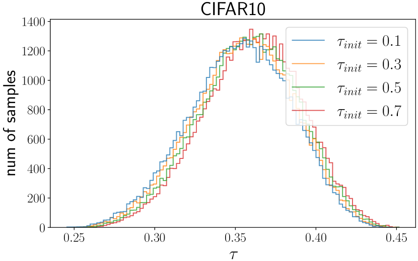
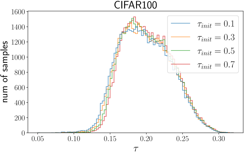
Refer to caption
Refer to caption
Refer to caption
Refer to caption
Refer to caption
Refer to caption
Refer to caption
Refer to caption
Figure 9: Distributions of the final learned temperatures with different τinitsubscript𝜏init\tau_{\text{init}} values on seven different datasets.

More results of the distributions of learned temperatures. We present the final distributions of the learned temperatures with different τinitsubscript𝜏init\tau_{\text{init}} values on all datasets in Figure 9. One can observe that the distributions for unimodal datasets are close to the Gaussian distribution. For CC3M dataset, we plot the distributions of learned temperatures of images and texts, respectively. We observe that these two distributions are very similar, and are close to the long-tail distribution with most samples have small temperatures.

More examples from CC3M dataset. We present more images and texts with large and small learned temperatures in Figure 10 and 11, respectively. One can observe that the images with large temperatures contain frequent semantics like person, house, animals, flowers, and natural landscape. While for images with small temperatures, their semantics could be abstract or rare in daily life.


Refer to caption
Figure 10: The images with large learned temperatures and their texts form CC3M. In general, they are very common in daily life, e.g., people, dogs, cats, flowers, houses, natural landscape, etc.
Refer to caption
Figure 11: The images with small learned temperatures and their texts form CC3M. Most of them are not common in our lives or contain abstract concepts.

Appendix D Convergence Analysis

We first introduce some notations. Let ||||||\cdot|| denote the Euclidean norm of a vector. We denote the combination of 𝐰𝐰\mathbf{w} and 𝝉𝝉\boldsymbol{\tau}, i.e., (𝐰,𝝉)d+nsuperscriptsuperscript𝐰topsuperscript𝝉toptopsuperscript𝑑𝑛(\mathbf{w}^{\top},\boldsymbol{\tau}^{\top})^{\top}\in\mathbb{R}^{d+n} by 𝐳𝐳\mathbf{z}. Recall that hi(𝐞)=E(𝒜(𝐱i))E(𝐞)E(𝒜(𝐱i))E(𝒜(𝐱i))subscript𝑖𝐞𝐸superscript𝒜subscript𝐱𝑖top𝐸𝐞𝐸superscript𝒜subscript𝐱𝑖top𝐸superscript𝒜subscript𝐱𝑖h_{i}(\mathbf{e})\!=\!E(\mathcal{A}(\mathbf{x}_{i}))^{\top}\!E(\mathbf{e})\!-\!E(\mathcal{A}(\mathbf{x}_{i}))^{\top}\!E(\mathcal{A}^{\prime}(\mathbf{x}_{i})), where we employ a new variable 𝐞𝐞\mathbf{e} in place of 𝐳𝐳\mathbf{z} used in (3) to avoid conflicts.

To simplify the notations, we use gi(𝐳)subscript𝑔𝑖𝐳g_{i}(\mathbf{z}) and gi(𝐳,)subscript𝑔𝑖𝐳g_{i}(\mathbf{z},\mathcal{B}) to represent gi(𝐰,𝝉i;𝒮i)subscript𝑔𝑖𝐰subscript𝝉𝑖superscriptsubscript𝒮𝑖g_{i}(\mathbf{w},\boldsymbol{\tau}_{i};\mathcal{S}_{i}^{-}) and gi(𝐰,𝝉i;i)subscript𝑔𝑖𝐰subscript𝝉𝑖subscript𝑖g_{i}(\mathbf{w},\boldsymbol{\tau}_{i};\mathcal{B}_{i}), respectively. We can see that 𝔼[gi(𝐳,)]=gi(𝐳)subscript𝔼delimited-[]subscript𝑔𝑖𝐳subscript𝑔𝑖𝐳\mathbb{E}_{\mathcal{B}}[g_{i}(\mathbf{z},\mathcal{B})]=g_{i}(\mathbf{z}). Then the objective (8) can be expressed as F(𝐳)=F(𝐰,𝝉)=1n𝐱i𝒟fi(𝝉i,gi(𝐳))𝐹𝐳𝐹𝐰𝝉1𝑛subscriptsubscript𝐱𝑖𝒟subscript𝑓𝑖subscript𝝉𝑖subscript𝑔𝑖𝐳F(\mathbf{z})=F(\mathbf{w},\boldsymbol{\tau})=\frac{1}{n}\sum_{\mathbf{x}_{i}\in\mathcal{D}}f_{i}(\boldsymbol{\tau}_{i},g_{i}(\mathbf{z})). We denote the batch sizes B=||𝐵B=|\mathcal{B}| and B=|i|superscript𝐵subscript𝑖B^{\prime}=|\mathcal{B}_{i}|.

Then we make the following standard assumptions regarding to problem (8).

Assumption 1.

There exists R,σ,Cg,Cf,Lf,Lg,C𝑅𝜎subscript𝐶𝑔subscript𝐶𝑓subscript𝐿𝑓subscript𝐿𝑔𝐶R,\sigma,C_{g},C_{f},L_{f},L_{g},C such that

  1. (i)

    The domain of model parameter 𝐰𝒲𝐰𝒲\mathbf{w}\in\mathcal{W} is bounded by R𝑅R, i.e., for all 𝐰𝒲𝐰𝒲\mathbf{w}\in\mathcal{W}, we have 𝐰Rnorm𝐰𝑅||\mathbf{w}||\leq R.

  2. (ii)

    𝔼[gi(𝐳)gi(𝐳,)2]σ2Bsubscript𝔼delimited-[]superscriptnormsubscript𝑔𝑖𝐳subscript𝑔𝑖𝐳2superscript𝜎2𝐵\mathbb{E}_{\mathcal{B}}[||g_{i}(\mathbf{z})-g_{i}(\mathbf{z},\mathcal{B})||^{2}]\leq\frac{\sigma^{2}}{B} and 𝔼[gi(𝐳)gi(𝐳,)2]σ2Bsubscript𝔼delimited-[]superscriptnormsubscript𝑔𝑖𝐳subscript𝑔𝑖𝐳2superscript𝜎2𝐵\mathbb{E}_{\mathcal{B}}[||\nabla g_{i}(\mathbf{z})-\nabla g_{i}(\mathbf{z},\mathcal{B})||^{2}]\leq\frac{\sigma^{2}}{B}.

  3. (iii)

    Functions gisubscript𝑔𝑖g_{i} and fisubscript𝑓𝑖f_{i} satisfy giCgnormsubscript𝑔𝑖subscript𝐶𝑔||\nabla g_{i}||\leq C_{g} and fiCfnormsubscript𝑓𝑖subscript𝐶𝑓||\nabla f_{i}||\leq C_{f} for all i𝑖i.

  4. (iv)

    Functions fi()subscript𝑓𝑖\nabla f_{i}(\cdot), gi()subscript𝑔𝑖\nabla g_{i}(\cdot) are Lfsubscript𝐿𝑓L_{f},Lgsubscript𝐿𝑔L_{g}-Lipschitz continuous for all i𝑖i.

  5. (v)

    Functions hi(𝐞)subscript𝑖𝐞h_{i}(\mathbf{e}) is bounded by C𝐶C for all i𝑖i, i.e., |hi(𝐞)|Csubscript𝑖𝐞𝐶|h_{i}(\mathbf{e})|\leq C.

Remark: Assumption 1(i)𝑖(i) is also assumed by Levy et al. (2020) and Qi et al. (2022), and is mainly used for convex analysis. Assumption 1(ii)𝑖𝑖(ii) assumes that the stochastic estimators of gi(𝐳)subscript𝑔𝑖𝐳g_{i}(\mathbf{z}) and gi(𝐳)subscript𝑔𝑖𝐳\nabla g_{i}(\mathbf{z}) have bounded variance. Assumption 1(iii)𝑖𝑖𝑖(iii) and (iv)𝑖𝑣(iv) are also standard for convergence analysis. Note that E(𝒜(𝐱i))𝐸𝒜subscript𝐱𝑖E\left(\mathcal{A}\left(\mathbf{x}_{i}\right)\right), E(𝒜(𝐱i))𝐸superscript𝒜subscript𝐱𝑖E\left(\mathcal{A}^{\prime}\left(\mathbf{x}_{i}\right)\right) and E(𝐞)𝐸𝐞E\left(\mathbf{e}\right) are all normalized vectors, thus their inner products are bounded and Assumption 1(v)𝑣(v) holds.

However, F(𝐰,𝝉)𝐹𝐰𝝉F(\mathbf{w},\boldsymbol{\tau}) is not necessarily smooth in terms of 𝐳=(𝐰,𝝉)𝐳superscriptsuperscript𝐰topsuperscript𝝉toptop\mathbf{z}=(\mathbf{w}^{\top},\boldsymbol{\tau}^{\top})^{\top} if 𝝉𝝉\boldsymbol{\tau} is unbounded. To address this concern, we have the following lemma:

Lemma 1.

The optimal solution of 𝛕i,i=1,2,,nformulae-sequencesuperscriptsubscript𝛕𝑖𝑖12𝑛\boldsymbol{\tau}_{i}^{*},i=1,2,\ldots,n to problem (8) is upper bounded by τ~=τ0+C/ρ~𝜏subscript𝜏0𝐶𝜌\tilde{\tau}=\tau_{0}+C/\rho, where C𝐶C is the upper bound for functions hi(𝐞)subscript𝑖𝐞h_{i}(\mathbf{e}) and ρ𝜌\rho is the constraint parameter.

Proof.

Recall the primal problem for each 𝐱i𝒟subscript𝐱𝑖𝒟\mathbf{x}_{i}\in\mathcal{D}:

𝐩=max{𝐩Δ,KL(𝐩,𝟏/m)ρ}𝐞j𝒮i𝐩jhi(𝐞j)τ0KL(𝐩,𝟏/m),superscript𝐩subscriptformulae-sequence𝐩ΔKL𝐩1𝑚𝜌subscriptsubscript𝐞𝑗superscriptsubscript𝒮𝑖subscript𝐩𝑗subscript𝑖subscript𝐞𝑗subscript𝜏0KL𝐩1𝑚\mathbf{p}^{*}=\max_{\{\mathbf{p}\in\Delta,\text{KL}(\mathbf{p},\boldsymbol{1}/m)\leq\rho\}}\sum_{\mathbf{e}_{j}\in\mathcal{S}_{i}^{-}}\mathbf{p}_{j}h_{i}(\mathbf{e}_{j})-\tau_{0}\text{KL}(\mathbf{p},\boldsymbol{1}/m),

where 𝐩superscript𝐩\mathbf{p}^{*} is the optimal value of the above problem.

Invoking dual variable λ¯isubscript¯𝜆𝑖\bar{\lambda}_{i}, we obtain the dual problem

𝐪=minλ¯0max𝐩Δ𝐞j𝒮i𝐩jhi(𝐞j)τ0KL(𝐩,𝟏/m)λ¯i(KL(𝐩,𝟏/m)ρ).superscript𝐪subscript¯𝜆0subscript𝐩Δsubscriptsubscript𝐞𝑗superscriptsubscript𝒮𝑖subscript𝐩𝑗subscript𝑖subscript𝐞𝑗subscript𝜏0KL𝐩1𝑚subscript¯𝜆𝑖KL𝐩1𝑚𝜌\mathbf{q}^{*}=\min_{\bar{\lambda}\geq 0}\max_{\mathbf{p}\in\Delta}\sum_{\mathbf{e}_{j}\in\mathcal{S}_{i}^{-}}\mathbf{p}_{j}h_{i}(\mathbf{e}_{j})-\tau_{0}\text{KL}(\mathbf{p},\boldsymbol{1}/m)-\bar{\lambda}_{i}\left(\text{KL}(\mathbf{p},\boldsymbol{1}/m)-\rho\right).

Set 𝐩¯=(1/m,,1/m)¯𝐩1𝑚1𝑚\bar{\mathbf{p}}=(1/m,\ldots,1/m), a Slater vector satisfying KL(𝐩¯,𝟏/m)ρ0KL¯𝐩1𝑚𝜌0\text{KL}(\bar{\mathbf{p}},\boldsymbol{1}/m)-\rho\leq 0. Applying Lemma 3 in (Nedić & Ozdaglar, 2009), we have

|λ¯i|1ρ(𝐪𝐞j𝒮i𝐩¯jhi(𝐞j)τ0KL(𝐩¯,𝟏/m)).superscriptsubscript¯𝜆𝑖1𝜌superscript𝐪subscriptsubscript𝐞𝑗superscriptsubscript𝒮𝑖subscript¯𝐩𝑗subscript𝑖subscript𝐞𝑗subscript𝜏0KL¯𝐩1𝑚|\bar{\lambda}_{i}^{*}|\leq\frac{1}{\rho}\left(\mathbf{q}^{*}-\sum_{\mathbf{e}_{j}\in\mathcal{S}_{i}^{-}}\bar{\mathbf{p}}_{j}h_{i}(\mathbf{e}_{j})-\tau_{0}\text{KL}(\bar{\mathbf{p}},\boldsymbol{1}/m)\right).

Since the primal problem is concave in terms of 𝐩𝐩\mathbf{p}, we have 𝐩=𝐪superscript𝐩superscript𝐪\mathbf{p}^{*}=\mathbf{q}^{*}. Therefore,

|λ¯i|superscriptsubscript¯𝜆𝑖\displaystyle|\bar{\lambda}_{i}^{*}| 1ρ(𝐩𝐞j𝒮i𝐩¯jhi(𝐞j))absent1𝜌superscript𝐩subscriptsubscript𝐞𝑗superscriptsubscript𝒮𝑖subscript¯𝐩𝑗subscript𝑖subscript𝐞𝑗\displaystyle\leq\frac{1}{\rho}\left(\mathbf{p}^{*}-\sum_{\mathbf{e}_{j}\in\mathcal{S}_{i}^{-}}\bar{\mathbf{p}}_{j}h_{i}(\mathbf{e}_{j})\right) (22)
1ρ(𝐞j𝒮i𝐩jhi(𝐞j)τ0D(𝐩,𝟏/m)𝐞j𝒮i𝐩¯jhi(𝐞j))absent1𝜌subscriptsubscript𝐞𝑗superscriptsubscript𝒮𝑖superscriptsubscript𝐩𝑗subscript𝑖subscript𝐞𝑗subscript𝜏0𝐷superscript𝐩1𝑚subscriptsubscript𝐞𝑗superscriptsubscript𝒮𝑖subscript¯𝐩𝑗subscript𝑖subscript𝐞𝑗\displaystyle\leq\frac{1}{\rho}\left(\sum_{\mathbf{e}_{j}\in\mathcal{S}_{i}^{-}}\mathbf{p}_{j}^{*}h_{i}(\mathbf{e}_{j})-\tau_{0}D(\mathbf{p}^{*},\boldsymbol{1}/m)-\sum_{\mathbf{e}_{j}\in\mathcal{S}_{i}^{-}}\bar{\mathbf{p}}_{j}h_{i}(\mathbf{e}_{j})\right)
Cρ,absent𝐶𝜌\displaystyle\leq\frac{C}{\rho},

where the last inequality is because |hi(𝐞j)|Csubscript𝑖subscript𝐞𝑗𝐶|h_{i}(\mathbf{e}_{j})|\leq C. Let 𝝉i=λ¯i+τ0subscript𝝉𝑖subscript¯𝜆𝑖subscript𝜏0\boldsymbol{\tau}_{i}=\bar{\lambda}_{i}+\tau_{0}, we have

𝐪=minττ0max𝐩Δ𝐞j𝒮i𝐩jhi(𝐞j)τ(KL(𝐩,𝟏/m)ρ)τ0ρ.superscript𝐪subscript𝜏subscript𝜏0subscript𝐩Δsubscriptsubscript𝐞𝑗superscriptsubscript𝒮𝑖subscript𝐩𝑗subscript𝑖subscript𝐞𝑗𝜏KL𝐩1𝑚𝜌subscript𝜏0𝜌\mathbf{q}^{*}=\min_{\tau\geq\tau_{0}}\max_{\mathbf{p}\in\Delta}\sum_{\mathbf{e}_{j}\in\mathcal{S}_{i}^{-}}\mathbf{p}_{j}h_{i}(\mathbf{e}_{j})-\tau\left(\text{KL}(\mathbf{p},\boldsymbol{1}/m)-\rho\right)-\tau_{0}\rho.

By (22), we know that the optimal solution for above problem |𝝉i||λ¯i|+τ0Cρ+τ0superscriptsubscript𝝉𝑖superscriptsubscript¯𝜆𝑖subscript𝜏0𝐶𝜌subscript𝜏0|\boldsymbol{\tau}_{i}^{*}|\leq|\bar{\lambda}_{i}^{*}|+\tau_{0}\leq\frac{C}{\rho}+\tau_{0}, which completes the proof.

Due the boundness of functions hi(𝐞)subscript𝑖𝐞h_{i}(\mathbf{e}) (cf. Assumption 1(v)𝑣(v)) and 𝝉isubscript𝝉𝑖\boldsymbol{\tau}_{i} (cf. Lemma 1), we have the following lemma:

Lemma 2.

Functions gi(𝐳t)subscript𝑔𝑖subscript𝐳𝑡g_{i}(\mathbf{z}_{t}) and gi(𝐳t,)subscript𝑔𝑖subscript𝐳𝑡g_{i}(\mathbf{z}_{t},\mathcal{B}) are lower bounded by g^=exp(C/τ~)^𝑔𝐶~𝜏\hat{g}=\exp(-C/\tilde{\tau}), where C𝐶-C is the lower bound for functions hi(𝐞)subscript𝑖𝐞h_{i}(\mathbf{e}) and τ~~𝜏\tilde{\tau} is the upper bound for 𝛕isuperscriptsubscript𝛕𝑖\boldsymbol{\tau}_{i}^{*}.

Proof.

Recall the definitions of hi(𝐞)subscript𝑖𝐞h_{i}(\mathbf{e}), gi(𝐳t)subscript𝑔𝑖subscript𝐳𝑡g_{i}(\mathbf{z}_{t}) and gi(𝐳t,)subscript𝑔𝑖subscript𝐳𝑡g_{i}(\mathbf{z}_{t},\mathcal{B}):

hi(𝐞)subscript𝑖𝐞\displaystyle h_{i}(\mathbf{e}) =E(𝒜(𝐱i))E(𝐞)E(𝒜(𝐱i))E(𝒜(𝐱i)),absent𝐸superscript𝒜subscript𝐱𝑖top𝐸𝐞𝐸superscript𝒜subscript𝐱𝑖top𝐸superscript𝒜subscript𝐱𝑖\displaystyle=\!E(\mathcal{A}(\mathbf{x}_{i}))^{\top}\!E(\mathbf{e})\!-\!E(\mathcal{A}(\mathbf{x}_{i}))^{\top}\!E(\mathcal{A}^{\prime}(\mathbf{x}_{i})),
gi(𝐳)subscript𝑔𝑖𝐳\displaystyle g_{i}(\mathbf{z}) =gi(𝐰,𝝉i;𝒮i)=1|𝒮i|𝐞𝒮iexp(hi(𝐞)𝝉i),absentsubscript𝑔𝑖𝐰subscript𝝉𝑖superscriptsubscript𝒮𝑖1superscriptsubscript𝒮𝑖subscript𝐞superscriptsubscript𝒮𝑖subscript𝑖𝐞subscript𝝉𝑖\displaystyle=g_{i}(\mathbf{w},\boldsymbol{\tau}_{i};\mathcal{S}_{i}^{-})=\frac{1}{|\mathcal{S}_{i}^{-}|}\sum_{\mathbf{e}\in\mathcal{S}_{i}^{-}}\exp\left(\frac{h_{i}(\mathbf{e})}{\boldsymbol{\tau}_{i}}\right),
gi(𝐳,)subscript𝑔𝑖𝐳\displaystyle g_{i}(\mathbf{z},\mathcal{B}) =gi(𝐰,𝝉i;i)=1i𝐞iexp(hi(𝐞)𝝉i).absentsubscript𝑔𝑖𝐰subscript𝝉𝑖subscript𝑖1subscript𝑖subscript𝐞subscript𝑖subscript𝑖𝐞subscript𝝉𝑖\displaystyle=g_{i}(\mathbf{w},\boldsymbol{\tau}_{i};\mathcal{B}_{i})=\frac{1}{\mathcal{B}_{i}}\sum_{\mathbf{e}\in\mathcal{B}_{i}}\exp\left(\frac{h_{i}(\mathbf{e})}{\boldsymbol{\tau}_{i}}\right).

Using 𝝉iτ~subscript𝝉𝑖~𝜏\boldsymbol{\tau}_{i}\leq\tilde{\tau} and hi(𝐞)Csubscript𝑖𝐞𝐶h_{i}(\mathbf{e})\geq-C, we have gi(𝐳)exp(Cτ~)subscript𝑔𝑖𝐳𝐶~𝜏g_{i}(\mathbf{z})\geq\exp\left(\frac{-C}{\tilde{\tau}}\right). Similarly, we have gi(𝐳,)exp(Cτ~)subscript𝑔𝑖𝐳𝐶~𝜏g_{i}(\mathbf{z},\mathcal{B})\geq\exp\left(\frac{-C}{\tilde{\tau}}\right), which completes the proof.

We will also see that the constraint on the domain of 𝝉𝝉\boldsymbol{\tau} guarantees the smoothness of F(𝐰,𝝉)𝐹𝐰𝝉F(\mathbf{w},\boldsymbol{\tau}), which is critical for the proposed algorithm to enjoy fast convergence rate.

Lemma 3.

For all 𝐰𝒲𝐰𝒲\mathbf{w}\in\mathcal{W}, 𝛕i[τ0,τ~]subscript𝛕𝑖subscript𝜏0~𝜏\boldsymbol{\tau}_{i}\in[\tau_{0},\tilde{\tau}], and i=1,2,,n𝑖12𝑛i=1,2,\dots,n, Fi(𝐳)=Fi(𝐰,𝛕i)=fi(𝛕i,gi(𝐳))subscript𝐹𝑖𝐳subscript𝐹𝑖𝐰subscript𝛕𝑖subscript𝑓𝑖subscript𝛕𝑖subscript𝑔𝑖𝐳F_{i}(\mathbf{z})=F_{i}(\mathbf{w},\boldsymbol{\tau}_{i})=f_{i}(\boldsymbol{\tau}_{i},g_{i}(\mathbf{z})) is LFsubscript𝐿𝐹L_{F}-smooth for some constant LFsubscript𝐿𝐹L_{F}.

Note that Lemma 3 naturally follows that function F(𝐳)𝐹𝐳F(\mathbf{z}) is also LFsubscript𝐿𝐹L_{F}-smooth.

Proof.

We have gradients

𝐰Fi(𝐰,𝝉i)subscript𝐰subscript𝐹𝑖𝐰subscript𝝉𝑖\displaystyle\nabla_{\mathbf{w}}F_{i}(\mathbf{w},\boldsymbol{\tau}_{i}) =𝐰gi(𝐰,𝝉i)gifi(𝝉i,gi(𝐰,𝝉i))absentsubscript𝐰subscript𝑔𝑖𝐰subscript𝝉𝑖subscriptsubscript𝑔𝑖subscript𝑓𝑖subscript𝝉𝑖subscript𝑔𝑖𝐰subscript𝝉𝑖\displaystyle=\nabla_{\mathbf{w}}g_{i}(\mathbf{w},\boldsymbol{\tau}_{i})\nabla_{g_{i}}f_{i}(\boldsymbol{\tau}_{i},g_{i}(\mathbf{w},\boldsymbol{\tau}_{i}))
=𝝉igi(𝐰,𝝉i)𝐰gi(𝐰,𝝉i)absentsubscript𝝉𝑖subscript𝑔𝑖𝐰subscript𝝉𝑖subscript𝐰subscript𝑔𝑖𝐰subscript𝝉𝑖\displaystyle=\frac{\boldsymbol{\tau}_{i}}{g_{i}(\mathbf{w},\boldsymbol{\tau}_{i})}\nabla_{\mathbf{w}}g_{i}(\mathbf{w},\boldsymbol{\tau}_{i})
𝝉Fi(𝐰,𝝉i)subscript𝝉subscript𝐹𝑖𝐰subscript𝝉𝑖\displaystyle\nabla_{\boldsymbol{\tau}}F_{i}(\mathbf{w},\boldsymbol{\tau}_{i}) =𝝉gi(𝐰,𝝉i)gifi(𝝉i,gi(𝐰,𝝉i))+𝝉fi(𝝉i,gi(𝐰,𝝉i))absentsubscript𝝉subscript𝑔𝑖𝐰subscript𝝉𝑖subscriptsubscript𝑔𝑖subscript𝑓𝑖subscript𝝉𝑖subscript𝑔𝑖𝐰subscript𝝉𝑖subscript𝝉subscript𝑓𝑖subscript𝝉𝑖subscript𝑔𝑖𝐰subscript𝝉𝑖\displaystyle=\nabla_{\boldsymbol{\tau}}g_{i}(\mathbf{w},\boldsymbol{\tau}_{i})\nabla_{g_{i}}f_{i}(\boldsymbol{\tau}_{i},g_{i}(\mathbf{w},\boldsymbol{\tau}_{i}))+\nabla_{\boldsymbol{\tau}}f_{i}(\boldsymbol{\tau}_{i},g_{i}(\mathbf{w},\boldsymbol{\tau}_{i}))
=𝝉igi(𝐰,𝝉i)𝝉gi(𝐰,𝝉i)+𝝉fi(𝝉i,gi(𝐰,𝝉i))absentsubscript𝝉𝑖subscript𝑔𝑖𝐰subscript𝝉𝑖subscript𝝉subscript𝑔𝑖𝐰subscript𝝉𝑖subscript𝝉subscript𝑓𝑖subscript𝝉𝑖subscript𝑔𝑖𝐰subscript𝝉𝑖\displaystyle=\frac{\boldsymbol{\tau}_{i}}{g_{i}(\mathbf{w},\boldsymbol{\tau}_{i})}\nabla_{\boldsymbol{\tau}}g_{i}(\mathbf{w},\boldsymbol{\tau}_{i})+\nabla_{\boldsymbol{\tau}}f_{i}(\boldsymbol{\tau}_{i},g_{i}(\mathbf{w},\boldsymbol{\tau}_{i}))
=𝝉igi(𝐰,𝝉i)(0𝝉igi(𝐰,𝝉i)0)+(0log(gi(𝐰,𝝉i))+ρ0)absentsubscript𝝉𝑖subscript𝑔𝑖𝐰subscript𝝉𝑖matrix0subscriptsubscript𝝉𝑖subscript𝑔𝑖𝐰subscript𝝉𝑖0matrix0subscript𝑔𝑖𝐰subscript𝝉𝑖𝜌0\displaystyle=\frac{\boldsymbol{\tau}_{i}}{g_{i}(\mathbf{w},\boldsymbol{\tau}_{i})}\begin{pmatrix}0\\ \vdots\\ \nabla_{\boldsymbol{\tau}_{i}}g_{i}(\mathbf{w},\boldsymbol{\tau}_{i})\\ \vdots\\ 0\\ \end{pmatrix}+\begin{pmatrix}0\\ \vdots\\ \log(g_{i}(\mathbf{w},\boldsymbol{\tau}_{i}))+\rho\\ \vdots\\ 0\\ \end{pmatrix}

For any arbitrary 𝐳,𝐳~𝐳~𝐳\mathbf{z},\tilde{\mathbf{z}}, we have

𝐳Fi(𝐳)𝐳Fi(𝐳~)2superscriptnormsubscript𝐳subscript𝐹𝑖𝐳subscript𝐳subscript𝐹𝑖~𝐳2\displaystyle\|\nabla_{\mathbf{z}}F_{i}(\mathbf{z})-\nabla_{\mathbf{z}}F_{i}(\tilde{\mathbf{z}})\|^{2}
=𝐰Fi(𝐳)𝐰Fi(𝐳~)2+𝝉Fi(𝐳)𝝉Fi(𝐳~)2absentsuperscriptnormsubscript𝐰subscript𝐹𝑖𝐳subscript𝐰subscript𝐹𝑖~𝐳2superscriptnormsubscript𝝉subscript𝐹𝑖𝐳subscript𝝉subscript𝐹𝑖~𝐳2\displaystyle=\|\nabla_{\mathbf{w}}F_{i}(\mathbf{z})-\nabla_{\mathbf{w}}F_{i}(\tilde{\mathbf{z}})\|^{2}+\|\nabla_{\boldsymbol{\tau}}F_{i}(\mathbf{z})-\nabla_{\boldsymbol{\tau}}F_{i}(\tilde{\mathbf{z}})\|^{2}
=𝝉igi(𝐰,𝝉i)𝐰gi(𝐰,𝝉i)𝝉~igi(𝐰~,𝝉~i)𝐰gi(𝐰~,𝝉~i)2absentsuperscriptnormsubscript𝝉𝑖subscript𝑔𝑖𝐰subscript𝝉𝑖subscript𝐰subscript𝑔𝑖𝐰subscript𝝉𝑖subscript~𝝉𝑖subscript𝑔𝑖~𝐰subscript~𝝉𝑖subscript𝐰subscript𝑔𝑖~𝐰subscript~𝝉𝑖2\displaystyle=\left\|\frac{\boldsymbol{\tau}_{i}}{g_{i}(\mathbf{w},\boldsymbol{\tau}_{i})}\nabla_{\mathbf{w}}g_{i}(\mathbf{w},\boldsymbol{\tau}_{i})-\frac{\tilde{\boldsymbol{\tau}}_{i}}{g_{i}(\tilde{\mathbf{w}},\tilde{\boldsymbol{\tau}}_{i})}\nabla_{\mathbf{w}}g_{i}(\tilde{\mathbf{w}},\tilde{\boldsymbol{\tau}}_{i})\right\|^{2}
+𝝉igi(𝐰,𝝉i)𝝉igi(𝐰,𝝉i)+log(gi(𝐰,𝝉i))(𝝉~igi(𝐰~,𝝉~i)𝝉igi(𝐰~,𝝉~i)+log(gi(𝐰~,𝝉~i)))2superscriptnormsubscript𝝉𝑖subscript𝑔𝑖𝐰subscript𝝉𝑖subscriptsubscript𝝉𝑖subscript𝑔𝑖𝐰subscript𝝉𝑖subscript𝑔𝑖𝐰subscript𝝉𝑖subscript~𝝉𝑖subscript𝑔𝑖~𝐰subscript~𝝉𝑖subscriptsubscript𝝉𝑖subscript𝑔𝑖~𝐰subscript~𝝉𝑖subscript𝑔𝑖~𝐰subscript~𝝉𝑖2\displaystyle\quad+\left\|\frac{\boldsymbol{\tau}_{i}}{g_{i}(\mathbf{w},\boldsymbol{\tau}_{i})}\nabla_{\boldsymbol{\tau}_{i}}g_{i}(\mathbf{w},\boldsymbol{\tau}_{i})+\log(g_{i}(\mathbf{w},\boldsymbol{\tau}_{i}))-\left(\frac{\tilde{\boldsymbol{\tau}}_{i}}{g_{i}(\tilde{\mathbf{w}},\tilde{\boldsymbol{\tau}}_{i})}\nabla_{\boldsymbol{\tau}_{i}}g_{i}(\tilde{\mathbf{w}},\tilde{\boldsymbol{\tau}}_{i})+\log(g_{i}(\tilde{\mathbf{w}},\tilde{\boldsymbol{\tau}}_{i}))\right)\right\|^{2}

Under assumption 1, we obtain

𝝉igi(𝐰,𝝉i)𝐰gi(𝐰,𝝉i)𝝉~igi(𝐰~,𝝉~i)𝐰gi(𝐰~,𝝉~i)2superscriptnormsubscript𝝉𝑖subscript𝑔𝑖𝐰subscript𝝉𝑖subscript𝐰subscript𝑔𝑖𝐰subscript𝝉𝑖subscript~𝝉𝑖subscript𝑔𝑖~𝐰subscript~𝝉𝑖subscript𝐰subscript𝑔𝑖~𝐰subscript~𝝉𝑖2\displaystyle\left\|\frac{\boldsymbol{\tau}_{i}}{g_{i}(\mathbf{w},\boldsymbol{\tau}_{i})}\nabla_{\mathbf{w}}g_{i}(\mathbf{w},\boldsymbol{\tau}_{i})-\frac{\tilde{\boldsymbol{\tau}}_{i}}{g_{i}(\tilde{\mathbf{w}},\tilde{\boldsymbol{\tau}}_{i})}\nabla_{\mathbf{w}}g_{i}(\tilde{\mathbf{w}},\tilde{\boldsymbol{\tau}}_{i})\right\|^{2}
2𝝉igi(𝐰,𝝉i)[𝐰gi(𝐰,𝝉i)𝐰gi(𝐰~,𝝉~i)]2+2[𝝉igi(𝐰,𝝉i)𝝉~igi(𝐰~,𝝉~i)]𝐰gi(𝐰~,𝝉~i)2absent2superscriptnormsubscript𝝉𝑖subscript𝑔𝑖𝐰subscript𝝉𝑖delimited-[]subscript𝐰subscript𝑔𝑖𝐰subscript𝝉𝑖subscript𝐰subscript𝑔𝑖~𝐰subscript~𝝉𝑖22superscriptnormdelimited-[]subscript𝝉𝑖subscript𝑔𝑖𝐰subscript𝝉𝑖subscript~𝝉𝑖subscript𝑔𝑖~𝐰subscript~𝝉𝑖subscript𝐰subscript𝑔𝑖~𝐰subscript~𝝉𝑖2\displaystyle\leq 2\left\|\frac{\boldsymbol{\tau}_{i}}{g_{i}(\mathbf{w},\boldsymbol{\tau}_{i})}\big{[}\nabla_{\mathbf{w}}g_{i}(\mathbf{w},\boldsymbol{\tau}_{i})-\nabla_{\mathbf{w}}g_{i}(\tilde{\mathbf{w}},\tilde{\boldsymbol{\tau}}_{i})\big{]}\right\|^{2}+2\left\|\left[\frac{\boldsymbol{\tau}_{i}}{g_{i}(\mathbf{w},\boldsymbol{\tau}_{i})}-\frac{\tilde{\boldsymbol{\tau}}_{i}}{g_{i}(\tilde{\mathbf{w}},\tilde{\boldsymbol{\tau}}_{i})}\right]\nabla_{\mathbf{w}}g_{i}(\tilde{\mathbf{w}},\tilde{\boldsymbol{\tau}}_{i})\right\|^{2}
2τ~Lgg^(𝐰𝐰~2+𝝉i𝝉~i2)+2τ~Cg2g^2(𝐰𝐰~2+𝝉i𝝉~i2)absent2~𝜏subscript𝐿𝑔^𝑔superscriptnorm𝐰~𝐰2superscriptnormsubscript𝝉𝑖subscript~𝝉𝑖22~𝜏superscriptsubscript𝐶𝑔2superscript^𝑔2superscriptnorm𝐰~𝐰2superscriptnormsubscript𝝉𝑖subscript~𝝉𝑖2\displaystyle\leq\frac{2\tilde{\tau}L_{g}}{\hat{g}}(\|\mathbf{w}-\tilde{\mathbf{w}}\|^{2}+\|\boldsymbol{\tau}_{i}-\tilde{\boldsymbol{\tau}}_{i}\|^{2})+\frac{2\tilde{\tau}C_{g}^{2}}{\hat{g}^{2}}(\|\mathbf{w}-\tilde{\mathbf{w}}\|^{2}+\|\boldsymbol{\tau}_{i}-\tilde{\boldsymbol{\tau}}_{i}\|^{2})

and

𝝉igi(𝐰,𝝉i)𝝉igi(𝐰,𝝉i)+log(gi(𝐰,𝝉i))(𝝉~igi(𝐰~,𝝉~i)𝝉igi(𝐰~,𝝉~i)+log(gi(𝐰~,𝝉~i)))2superscriptnormsubscript𝝉𝑖subscript𝑔𝑖𝐰subscript𝝉𝑖subscriptsubscript𝝉𝑖subscript𝑔𝑖𝐰subscript𝝉𝑖subscript𝑔𝑖𝐰subscript𝝉𝑖subscript~𝝉𝑖subscript𝑔𝑖~𝐰subscript~𝝉𝑖subscriptsubscript𝝉𝑖subscript𝑔𝑖~𝐰subscript~𝝉𝑖subscript𝑔𝑖~𝐰subscript~𝝉𝑖2\displaystyle\left\|\frac{\boldsymbol{\tau}_{i}}{g_{i}(\mathbf{w},\boldsymbol{\tau}_{i})}\nabla_{\boldsymbol{\tau}_{i}}g_{i}(\mathbf{w},\boldsymbol{\tau}_{i})+\log(g_{i}(\mathbf{w},\boldsymbol{\tau}_{i}))-\left(\frac{\tilde{\boldsymbol{\tau}}_{i}}{g_{i}(\tilde{\mathbf{w}},\tilde{\boldsymbol{\tau}}_{i})}\nabla_{\boldsymbol{\tau}_{i}}g_{i}(\tilde{\mathbf{w}},\tilde{\boldsymbol{\tau}}_{i})+\log(g_{i}(\tilde{\mathbf{w}},\tilde{\boldsymbol{\tau}}_{i}))\right)\right\|^{2}
4(Cgg^+τ~Cg2g^2+τ~Lgg^+Cgg^)(𝐰𝐰~2+𝝉i𝝉~i2)absent4subscript𝐶𝑔^𝑔~𝜏superscriptsubscript𝐶𝑔2superscript^𝑔2~𝜏subscript𝐿𝑔^𝑔subscript𝐶𝑔^𝑔superscriptnorm𝐰~𝐰2superscriptnormsubscript𝝉𝑖subscript~𝝉𝑖2\displaystyle\leq 4\left(\frac{C_{g}}{\hat{g}}+\frac{\tilde{\tau}C_{g}^{2}}{\hat{g}^{2}}+\frac{\tilde{\tau}L_{g}}{\hat{g}}+\frac{C_{g}}{\hat{g}}\right)(\|\mathbf{w}-\tilde{\mathbf{w}}\|^{2}+\|\boldsymbol{\tau}_{i}-\tilde{\boldsymbol{\tau}}_{i}\|^{2})

Define LF=2τ~Lgg^+2τ~Cg2g^2+4(Cgg^+τ~Cg2g^2+τ~Lgg^+Cgg^)subscript𝐿𝐹2~𝜏subscript𝐿𝑔^𝑔2~𝜏superscriptsubscript𝐶𝑔2superscript^𝑔24subscript𝐶𝑔^𝑔~𝜏superscriptsubscript𝐶𝑔2superscript^𝑔2~𝜏subscript𝐿𝑔^𝑔subscript𝐶𝑔^𝑔L_{F}=\frac{2\tilde{\tau}L_{g}}{\hat{g}}+\frac{2\tilde{\tau}C_{g}^{2}}{\hat{g}^{2}}+4\left(\frac{C_{g}}{\hat{g}}+\frac{\tilde{\tau}C_{g}^{2}}{\hat{g}^{2}}+\frac{\tilde{\tau}L_{g}}{\hat{g}}+\frac{C_{g}}{\hat{g}}\right), then 𝐳Fi(𝐳)𝐳Fi(𝐳~)2Lf𝐳𝐳~2superscriptnormsubscript𝐳subscript𝐹𝑖𝐳subscript𝐳subscript𝐹𝑖~𝐳2subscript𝐿𝑓superscriptnorm𝐳~𝐳2\|\nabla_{\mathbf{z}}F_{i}(\mathbf{z})-\nabla_{\mathbf{z}}F_{i}(\tilde{\mathbf{z}})\|^{2}\leq L_{f}\|\mathbf{z}-\tilde{\mathbf{z}}\|^{2}. ∎

Below, we let χ={𝐳|𝐰𝒲,τ0𝝉iτ~,i=1,2,,n}𝜒conditional-set𝐳formulae-sequenceformulae-sequence𝐰𝒲subscript𝜏0subscript𝝉𝑖~𝜏𝑖12𝑛\chi=\{\mathbf{z}|\mathbf{w}\in\mathcal{W},\tau_{0}\leq\boldsymbol{\tau}_{i}\leq\tilde{\tau},i=1,2,\ldots,n\}. δχ(𝐳)=0subscript𝛿𝜒𝐳0\delta_{\chi}(\mathbf{z})=0 if 𝐳χ𝐳𝜒\mathbf{z}\in\chi, and δχ(𝐳)=subscript𝛿𝜒𝐳\delta_{\chi}(\mathbf{z})=\infty if 𝐳χ𝐳𝜒\mathbf{z}\notin\chi. Then problem (8) is equivalent to:

min𝐳d+nF¯(𝐳):=F(𝐳)+δχ(𝐳).assignsubscript𝐳superscript𝑑𝑛¯𝐹𝐳𝐹𝐳subscript𝛿𝜒𝐳\min_{\mathbf{z}\in\mathbb{R}^{d+n}}\bar{F}(\mathbf{z}):=F(\mathbf{z})+\delta_{\chi}(\mathbf{z}). (23)

Now the update step of 𝐳tsubscript𝐳𝑡\mathbf{z}_{t} can be written as 𝐳t+1=Πχ(𝐳tη𝐝t+1)subscript𝐳𝑡1subscriptΠ𝜒subscript𝐳𝑡𝜂subscript𝐝𝑡1\mathbf{z}_{t+1}=\Pi_{\chi}(\mathbf{z}_{t}-\eta\mathbf{d}_{t+1}), where ΠχsubscriptΠ𝜒\Pi_{\chi} denotes the Euclidean projection onto the domain χ𝜒\chi, and 𝐝t+1=(𝐯t+1,𝐮t+1)subscript𝐝𝑡1superscriptsuperscriptsubscript𝐯𝑡1topsuperscriptsuperscript𝐮𝑡1toptop\mathbf{d}_{t+1}=(\mathbf{v}_{t+1}^{\top},{\mathbf{u}^{t+1}}^{\top})^{\top}.

Since F¯¯𝐹\bar{F} is non-smooth, we define the regular subgradients as follows.

Definition 1 (Regular Subgradient).

Consider a function Φ:n¯:Φsuperscript𝑛¯\Phi:\mathbb{R}^{n}\rightarrow\bar{\mathbb{R}} and Φ(𝐱¯)Φ¯𝐱\Phi(\bar{\mathbf{x}}) is finite. For a vector 𝐯n𝐯superscript𝑛\mathbf{v}\in\mathbb{R}^{n}, 𝐯𝐯\mathbf{v} is a regular subgradient of ΦΦ\Phi at 𝐱¯¯𝐱\bar{\mathbf{x}}, written 𝐯^Φ(𝐱¯)𝐯^Φ¯𝐱\mathbf{v}\in\hat{\partial}\Phi(\bar{\mathbf{x}}), if

lim inf𝐱𝐱¯Φ(𝐱)Φ(𝐱¯)𝐯(𝐱𝐱¯)𝐱𝐱¯0.subscriptlimit-infimum𝐱¯𝐱Φ𝐱Φ¯𝐱superscript𝐯top𝐱¯𝐱norm𝐱¯𝐱0\liminf_{\mathbf{x}\rightarrow\overline{\mathbf{x}}}\frac{\Phi(\mathbf{x})-\Phi(\overline{\mathbf{x}})-\mathbf{v}^{\top}(\mathbf{x}-\overline{\mathbf{x}})}{\|\mathbf{x}-\overline{\mathbf{x}}\|}\geq 0.

Since F(𝐳)𝐹𝐳F(\mathbf{z}) is differentiable, we use ^F¯(𝐳)=F(𝐳)+^δχ(𝐳)^¯𝐹𝐳𝐹𝐳^subscript𝛿𝜒𝐳\hat{\partial}\bar{F}(\mathbf{z})=\nabla F(\mathbf{z})+\hat{\partial}\delta_{\chi}(\mathbf{z}) (see Exercise 8.8 in Rockafellar & Wets (2009)) in the analysis. The dist(0,^F¯(𝐳))dist0^¯𝐹𝐳\text{dist}(0,\hat{\partial}\bar{F}(\mathbf{z})) measures the distance between the origin and the regular subgradient set of F¯¯𝐹\bar{F} at 𝐳𝐳\mathbf{z}. The oracle complexity is defined below:

Definition 2 (Oracle Complexity).

Let ϵ>0italic-ϵ0\epsilon>0 be a small constant, the oracle complexity is defined as the number of processing samples in order to achieve 𝔼[dist(0,^F¯(𝐳))]ϵ𝔼delimited-[]dist0^¯𝐹𝐳italic-ϵ\mathbb{E}[\text{dist}(0,\hat{\partial}\bar{F}(\mathbf{z}))]\leq\epsilon for a non-convex loss function or 𝔼[F(𝐳)F(𝐳)]ϵ𝔼delimited-[]𝐹𝐳𝐹subscript𝐳italic-ϵ\mathbb{E}[F(\mathbf{z})-F(\mathbf{z}_{*})]\leq\epsilon for a convex loss function.

To prove the main theorem, we present some required lemmas.

Lemma 4.

Under Assumption 1, run Algorithm 1 with ηLF14𝜂subscript𝐿𝐹14\eta L_{F}\leq\frac{1}{4}, and the output 𝐳Rsubscript𝐳𝑅\mathbf{z}_{R} of Algorithm 1 satisfies

𝔼[dist(0,^F¯(𝐳R))]2+40LFηTt=1T𝐝t+1F(𝐳t)2+2ΔηT+40LFΔT,𝔼delimited-[]𝑑𝑖𝑠𝑡0^¯𝐹subscript𝐳𝑅240subscript𝐿𝐹𝜂𝑇superscriptsubscript𝑡1𝑇superscriptnormsubscript𝐝𝑡1𝐹subscript𝐳𝑡22Δ𝜂𝑇40subscript𝐿𝐹Δ𝑇\mathbb{E}[dist(0,\hat{\partial}\bar{F}(\mathbf{z}_{R}))]\leq\frac{2+40L_{F}\eta}{T}\sum_{t=1}^{T}||\mathbf{d}_{t+1}-\nabla F(\mathbf{z}_{t})||^{2}+\frac{2\Delta}{\eta T}+\frac{40L_{F}\Delta}{T},

where Δ:=F¯(𝐳1)inf𝐳χF¯(𝐳)assignΔ¯𝐹subscript𝐳1subscriptinfimum𝐳𝜒¯𝐹𝐳\Delta:=\bar{F}(\mathbf{z}_{1})-\inf_{\mathbf{z}\in\chi}\bar{F}(\mathbf{z}).

Proof.

Recall the update of 𝐳t+1subscript𝐳𝑡1\mathbf{z}_{t+1} is

𝐳t+1subscript𝐳𝑡1\displaystyle\mathbf{z}_{t+1} =Πχ(𝐳tη𝐝t+1)absentsubscriptΠ𝜒subscript𝐳𝑡𝜂subscript𝐝𝑡1\displaystyle=\Pi_{\chi}(\mathbf{z}_{t}-\eta\mathbf{d}_{t+1})
=argmin𝐳d+n{δχ(𝐳)+𝐝t+1,𝐳𝐳t+12η𝐳𝐳t2}.absentsubscriptargmin𝐳superscript𝑑𝑛subscript𝛿𝜒𝐳subscript𝐝𝑡1𝐳subscript𝐳𝑡12𝜂superscriptnorm𝐳subscript𝐳𝑡2\displaystyle=\operatorname*{arg\,min}_{\mathbf{z}\in\mathbb{R}^{d+n}}\left\{\delta_{\chi}(\mathbf{z})+\langle\mathbf{d}_{t+1},\mathbf{z}-\mathbf{z}_{t}\rangle+\frac{1}{2\eta}||\mathbf{z}-\mathbf{z}_{t}||^{2}\right\}.

Then by Exercise 8.8 and Theorem 10.1 of Rockafellar & Wets (2009), we know

𝐝t+11η(𝐳t+1𝐳t)^δχ(𝐳t+1),subscript𝐝𝑡11𝜂subscript𝐳𝑡1subscript𝐳𝑡^subscript𝛿𝜒subscript𝐳𝑡1-\mathbf{d}_{t+1}-\frac{1}{\eta}(\mathbf{z}_{t+1}-\mathbf{z}_{t})\in\hat{\partial}\delta_{\chi}(\mathbf{z}_{t+1}),

which implies that

F(𝐳t+1)𝐝t+11η(𝐳t+1𝐳t)F(𝐳t+1)+^δχ(𝐳t+1)=^F¯(𝐳t+1).𝐹subscript𝐳𝑡1subscript𝐝𝑡11𝜂subscript𝐳𝑡1subscript𝐳𝑡𝐹subscript𝐳𝑡1^subscript𝛿𝜒subscript𝐳𝑡1^¯𝐹subscript𝐳𝑡1\nabla F(\mathbf{z}_{t+1})-\mathbf{d}_{t+1}-\frac{1}{\eta}(\mathbf{z}_{t+1}-\mathbf{z}_{t})\in\nabla F(\mathbf{z}_{t+1})+\hat{\partial}\delta_{\chi}(\mathbf{z}_{t+1})=\hat{\partial}\bar{F}(\mathbf{z}_{t+1}). (24)

By the update of 𝐳t+1subscript𝐳𝑡1\mathbf{z}_{t+1}, we also have

δχ(𝐳t+1)+𝐝t+1,𝐳t+1𝐳t+12η𝐳t+1𝐳t2δχ(𝐳t).subscript𝛿𝜒subscript𝐳𝑡1subscript𝐝𝑡1subscript𝐳𝑡1subscript𝐳𝑡12𝜂superscriptnormsubscript𝐳𝑡1subscript𝐳𝑡2subscript𝛿𝜒subscript𝐳𝑡\delta_{\chi}(\mathbf{z}_{t+1})+\langle\mathbf{d}_{t+1},\mathbf{z}_{t+1}-\mathbf{z}_{t}\rangle+\frac{1}{2\eta}||\mathbf{z}_{t+1}-\mathbf{z}_{t}||^{2}\leq\delta_{\chi}(\mathbf{z}_{t}).

Since F(𝐳)𝐹𝐳F(\mathbf{z}) is LFsubscript𝐿𝐹L_{F}-smooth, we have

F(𝐳t+1)F(𝐳t)+F(𝐳t),𝐳t+1𝐳t+LF2𝐳t+1𝐳t2.𝐹subscript𝐳𝑡1𝐹subscript𝐳𝑡𝐹subscript𝐳𝑡subscript𝐳𝑡1subscript𝐳𝑡subscript𝐿𝐹2superscriptnormsubscript𝐳𝑡1subscript𝐳𝑡2F(\mathbf{z}_{t+1})\leq F(\mathbf{z}_{t})+\langle\nabla F(\mathbf{z}_{t}),\mathbf{z}_{t+1}-\mathbf{z}_{t}\rangle+\frac{L_{F}}{2}||\mathbf{z}_{t+1}-\mathbf{z}_{t}||^{2}.

Combining the above two inequalities, we obtain

𝐝t+1F(𝐳t),𝐳t+1𝐳t+12(1ηLF)𝐳t+1𝐳t2F¯(𝐳t)F¯(𝐳t+1).subscript𝐝𝑡1𝐹subscript𝐳𝑡subscript𝐳𝑡1subscript𝐳𝑡121𝜂subscript𝐿𝐹superscriptnormsubscript𝐳𝑡1subscript𝐳𝑡2¯𝐹subscript𝐳𝑡¯𝐹subscript𝐳𝑡1\langle\mathbf{d}_{t+1}-\nabla F(\mathbf{z}_{t}),\mathbf{z}_{t+1}-\mathbf{z}_{t}\rangle+\frac{1}{2}\left(\frac{1}{\eta}-L_{F}\right)||\mathbf{z}_{t+1}-\mathbf{z}_{t}||^{2}\leq\bar{F}(\mathbf{z}_{t})-\bar{F}(\mathbf{z}_{t+1}).

Thus we have

12(1ηLF)𝐳t+1𝐳t2F¯(𝐳t)F¯(𝐳t+1)𝐝t+1F(𝐳t),𝐳t+1𝐳t,121𝜂subscript𝐿𝐹superscriptnormsubscript𝐳𝑡1subscript𝐳𝑡2¯𝐹subscript𝐳𝑡¯𝐹subscript𝐳𝑡1subscript𝐝𝑡1𝐹subscript𝐳𝑡subscript𝐳𝑡1subscript𝐳𝑡\frac{1}{2}\left(\frac{1}{\eta}-L_{F}\right)||\mathbf{z}_{t+1}-\mathbf{z}_{t}||^{2}\leq\bar{F}(\mathbf{z}_{t})-\bar{F}(\mathbf{z}_{t+1})-\langle\mathbf{d}_{t+1}-\nabla F(\mathbf{z}_{t}),\mathbf{z}_{t+1}-\mathbf{z}_{t}\rangle,

where the last inequality uses 𝐚,𝐛𝐚2+𝐛24𝐚𝐛superscriptnorm𝐚2superscriptnorm𝐛24\langle\mathbf{a},\mathbf{b}\rangle\leq||\mathbf{a}||^{2}+\frac{||\mathbf{b}||^{2}}{4}. Then by rearranging the above inequality and summing it across t=1,2,,T𝑡12𝑇t=1,2,\ldots,T, we have

t=1T12ηLF4η𝐳t+1𝐳t2superscriptsubscript𝑡1𝑇12𝜂subscript𝐿𝐹4𝜂superscriptnormsubscript𝐳𝑡1subscript𝐳𝑡2\displaystyle\sum_{t=1}^{T}\frac{1-2\eta L_{F}}{4\eta}||\mathbf{z}_{t+1}-\mathbf{z}_{t}||^{2} F¯(𝐳1)F¯(𝐳T+1)+t=1Tη𝐝t+1F(𝐳t)2absent¯𝐹subscript𝐳1¯𝐹subscript𝐳𝑇1superscriptsubscript𝑡1𝑇𝜂superscriptnormsubscript𝐝𝑡1𝐹subscript𝐳𝑡2\displaystyle\leq\bar{F}(\mathbf{z}_{1})-\bar{F}(\mathbf{z}_{T+1})+\sum_{t=1}^{T}\eta||\mathbf{d}_{t+1}-\nabla F(\mathbf{z}_{t})||^{2} (25)
F¯(𝐳1)inf𝐳χF¯(𝐳)+t=1Tη𝐝t+1F(𝐳t)2absent¯𝐹subscript𝐳1subscriptinfimum𝐳𝜒¯𝐹𝐳superscriptsubscript𝑡1𝑇𝜂superscriptnormsubscript𝐝𝑡1𝐹subscript𝐳𝑡2\displaystyle\leq\bar{F}(\mathbf{z}_{1})-\inf_{\mathbf{z}\in\chi}\bar{F}(\mathbf{z})+\sum_{t=1}^{T}\eta||\mathbf{d}_{t+1}-\nabla F(\mathbf{z}_{t})||^{2}
=Δ+t=1Tη𝐝t+1F(𝐳t)2absentΔsuperscriptsubscript𝑡1𝑇𝜂superscriptnormsubscript𝐝𝑡1𝐹subscript𝐳𝑡2\displaystyle=\Delta+\sum_{t=1}^{T}\eta||\mathbf{d}_{t+1}-\nabla F(\mathbf{z}_{t})||^{2}

Using the same method in the proof of Theorem 2 in (Xu et al., 2019), we obtain the following relationship:

t=1T𝐝t+1F(𝐳t+1)+1η(𝐳t+1𝐳t)2superscriptsubscript𝑡1𝑇superscriptnormsubscript𝐝𝑡1𝐹subscript𝐳𝑡11𝜂subscript𝐳𝑡1subscript𝐳𝑡2\displaystyle\sum_{t=1}^{T}||\mathbf{d}_{t+1}-\nabla F(\mathbf{z}_{t+1})+\frac{1}{\eta}(\mathbf{z}_{t+1}-\mathbf{z}_{t})||^{2} 2t=1T𝐝t+1F(𝐳t)2+2Δηabsent2superscriptsubscript𝑡1𝑇superscriptnormsubscript𝐝𝑡1𝐹subscript𝐳𝑡22Δ𝜂\displaystyle\leq 2\sum_{t=1}^{T}||\mathbf{d}_{t+1}-\nabla F(\mathbf{z}_{t})||^{2}+\frac{2\Delta}{\eta} (26)
+(2LF2+3LFη)t=1T𝐳t+1𝐳t22superscriptsubscript𝐿𝐹23subscript𝐿𝐹𝜂superscriptsubscript𝑡1𝑇superscriptnormsubscript𝐳𝑡1subscript𝐳𝑡2\displaystyle+\left(2L_{F}^{2}+\frac{3L_{F}}{\eta}\right)\sum_{t=1}^{T}||\mathbf{z}_{t+1}-\mathbf{z}_{t}||^{2}

Recalling ηLF14𝜂subscript𝐿𝐹14\eta L_{F}\leq\frac{1}{4} and combining (25) and (26), we have

t=1T𝐝t+1F(𝐳t+1)+1η(𝐳t+1𝐳t)2superscriptsubscript𝑡1𝑇superscriptnormsubscript𝐝𝑡1𝐹subscript𝐳𝑡11𝜂subscript𝐳𝑡1subscript𝐳𝑡2\displaystyle\sum_{t=1}^{T}||\mathbf{d}_{t+1}-\nabla F(\mathbf{z}_{t+1})+\frac{1}{\eta}(\mathbf{z}_{t+1}-\mathbf{z}_{t})||^{2} (27)
(a)2t=1T𝐝t+1F(𝐳t)2+2Δη+5LFη(412ηLF)(ηΔ+t=1Tη2𝐝t+1F(𝐳t)2)superscript𝑎absent2superscriptsubscript𝑡1𝑇superscriptnormsubscript𝐝𝑡1𝐹subscript𝐳𝑡22Δ𝜂5subscript𝐿𝐹𝜂412𝜂subscript𝐿𝐹𝜂Δsuperscriptsubscript𝑡1𝑇superscript𝜂2superscriptnormsubscript𝐝𝑡1𝐹subscript𝐳𝑡2\displaystyle\stackrel{{\scriptstyle(a)}}{{\leq}}2\sum_{t=1}^{T}||\mathbf{d}_{t+1}-\nabla F(\mathbf{z}_{t})||^{2}+\frac{2\Delta}{\eta}+\frac{5L_{F}}{\eta}\left(\frac{4}{1-2\eta L_{F}}\right)\left(\eta\Delta+\sum_{t=1}^{T}\eta^{2}||\mathbf{d}_{t+1}-\nabla F(\mathbf{z}_{t})||^{2}\right)
(b)2t=1T𝐝t+1F(𝐳t)2+2Δη+40LFΔ+40ηLFt=1T𝐝t+1F(𝐳t)2,superscript𝑏absent2superscriptsubscript𝑡1𝑇superscriptnormsubscript𝐝𝑡1𝐹subscript𝐳𝑡22Δ𝜂40subscript𝐿𝐹Δ40𝜂subscript𝐿𝐹superscriptsubscript𝑡1𝑇superscriptnormsubscript𝐝𝑡1𝐹subscript𝐳𝑡2\displaystyle\stackrel{{\scriptstyle(b)}}{{\leq}}2\sum_{t=1}^{T}||\mathbf{d}_{t+1}-\nabla F(\mathbf{z}_{t})||^{2}+\frac{2\Delta}{\eta}+40L_{F}\Delta+40\eta L_{F}\sum_{t=1}^{T}||\mathbf{d}_{t+1}-\nabla F(\mathbf{z}_{t})||^{2},

where (a) is due to (2LF2+3LFη)5LFη2superscriptsubscript𝐿𝐹23subscript𝐿𝐹𝜂5subscript𝐿𝐹𝜂(2L_{F}^{2}+\frac{3L_{F}}{\eta})\leq\frac{5L_{F}}{\eta} and (b) is due to 412ηLF8412𝜂subscript𝐿𝐹8\frac{4}{1-2\eta L_{F}}\leq 8.

Recalling (24) and the output rule of Algorithm 1, we have

𝔼[dist(0,^F¯(𝐳R))2]1Tt=1T𝔼[𝐝t+1F(𝐳t+1)+1η(𝐳t+1𝐳t)2].𝔼delimited-[]distsuperscript0^¯𝐹subscript𝐳𝑅21𝑇superscriptsubscript𝑡1𝑇𝔼delimited-[]superscriptnormsubscript𝐝𝑡1𝐹subscript𝐳𝑡11𝜂subscript𝐳𝑡1subscript𝐳𝑡2\mathbb{E}[\text{dist}(0,\hat{\partial}\bar{F}(\mathbf{z}_{R}))^{2}]\leq\frac{1}{T}\sum_{t=1}^{T}\mathbb{E}[||\mathbf{d}_{t+1}-\nabla F(\mathbf{z}_{t+1})+\frac{1}{\eta}(\mathbf{z}_{t+1}-\mathbf{z}_{t})||^{2}]. (28)

At last, we combine (27) and (28) and have

𝔼[dist(0,^F¯(𝐳R))2]2+40ηLFTt=1T𝔼[𝐝t+1F(𝐳t)2]+2ΔTη+40LFΔT.𝔼delimited-[]distsuperscript0^¯𝐹subscript𝐳𝑅2240𝜂subscript𝐿𝐹𝑇superscriptsubscript𝑡1𝑇𝔼delimited-[]superscriptnormsubscript𝐝𝑡1𝐹subscript𝐳𝑡22Δ𝑇𝜂40subscript𝐿𝐹Δ𝑇\mathbb{E}[\text{dist}(0,\hat{\partial}\bar{F}(\mathbf{z}_{R}))^{2}]\leq\frac{2+40\eta L_{F}}{T}\sum_{t=1}^{T}\mathbb{E}[||\mathbf{d}_{t+1}-\nabla F(\mathbf{z}_{t})||^{2}]+\frac{2\Delta}{T\eta}+\frac{40L_{F}\Delta}{T}. (29)

Lemma 5.

Under Assumption 1, run Algorithm 1 and we have

t=1T𝔼[𝐝t+1F(𝐳t)2]superscriptsubscript𝑡1𝑇𝔼delimited-[]superscriptnormsubscript𝐝𝑡1𝐹subscript𝐳𝑡2\displaystyle\sum_{t=1}^{T}\mathbb{E}[||\mathbf{d}_{t+1}-\nabla F(\mathbf{z}_{t})||^{2}] Δ𝐯+Δ𝐮+(4LF2β12+72n3LF2B2β2)t=1T𝔼[𝐳t𝐳t12]absentsubscriptΔ𝐯subscriptΔ𝐮4superscriptsubscript𝐿𝐹2superscriptsubscript𝛽1272superscript𝑛3superscriptsubscript𝐿𝐹2superscript𝐵2superscript𝛽2superscriptsubscript𝑡1𝑇𝔼delimited-[]superscriptnormsubscript𝐳𝑡subscript𝐳𝑡12\displaystyle\leq\Delta_{\mathbf{v}}+\Delta_{\mathbf{u}}+\left(\frac{4L_{F}^{2}}{\beta_{1}^{2}}+\frac{72n^{3}L_{F}^{2}}{B^{2}\beta^{2}}\right)\sum_{t=1}^{T}\mathbb{E}[||\mathbf{z}_{t}-\mathbf{z}_{t-1}||^{2}]
+C1t=1T𝔼[g(𝐳t)𝐬t+12]+C2β1BT+C3βBT,subscript𝐶1superscriptsubscript𝑡1𝑇𝔼delimited-[]superscriptnorm𝑔subscript𝐳𝑡superscript𝐬𝑡12subscript𝐶2subscript𝛽1𝐵𝑇subscript𝐶3𝛽𝐵𝑇\displaystyle\quad+C_{1}\sum_{t=1}^{T}\mathbb{E}[||g(\mathbf{z}_{t})-\mathbf{s}^{t+1}||^{2}]+\frac{C_{2}\beta_{1}}{B}T+\frac{C_{3}\beta}{B}T,

where Δ𝐯,Δ𝐮,C1,C2,C3subscriptΔ𝐯subscriptΔ𝐮subscript𝐶1subscript𝐶2subscript𝐶3\Delta_{\mathbf{v}},\Delta_{\mathbf{u}},C_{1},C_{2},C_{3} are constants defined in the proof.

Proof.

Recalling 𝐝t+1=(𝐯t+1,𝐮t+1)subscript𝐝𝑡1superscriptsuperscriptsubscript𝐯𝑡1topsuperscriptsuperscript𝐮𝑡1toptop\mathbf{d}_{t+1}=(\mathbf{v}_{t+1}^{\top},{\mathbf{u}^{t+1}}^{\top})^{\top} and F(𝐳t)=(𝐰F(𝐳t),𝝉F(𝐳t))𝐹subscript𝐳𝑡superscriptsubscript𝐰𝐹subscript𝐳𝑡subscript𝝉𝐹subscript𝐳𝑡top\nabla F(\mathbf{z}_{t})=(\nabla_{\mathbf{w}}F(\mathbf{z}_{t}),\nabla_{\boldsymbol{\tau}}F(\mathbf{z}_{t}))^{\top}, we have

𝐝t+1F(𝐳t)2=𝐯t+1𝐰F(𝐳t)2+𝐮t+1𝝉F(𝐳t)2superscriptnormsubscript𝐝𝑡1𝐹subscript𝐳𝑡2superscriptnormsubscript𝐯𝑡1subscript𝐰𝐹subscript𝐳𝑡2superscriptnormsuperscript𝐮𝑡1subscript𝝉𝐹subscript𝐳𝑡2||\mathbf{d}_{t+1}-\nabla F(\mathbf{z}_{t})||^{2}=||\mathbf{v}_{t+1}-\nabla_{\mathbf{w}}F(\mathbf{z}_{t})||^{2}+||\mathbf{u}^{t+1}-\nabla_{\boldsymbol{\tau}}F(\mathbf{z}_{t})||^{2}

We first establish the bound for 𝐯t+1𝐰F(𝐳t)2superscriptnormsubscript𝐯𝑡1subscript𝐰𝐹subscript𝐳𝑡2||\mathbf{v}_{t+1}-\nabla_{\mathbf{w}}F(\mathbf{z}_{t})||^{2}. Recall the define the following notations

F(𝐳t)=1n𝐱i𝒮𝐰fi(gi(𝐳t))𝐰gi(𝐳t),𝐹subscript𝐳𝑡1𝑛subscriptsubscript𝐱𝑖𝒮subscript𝐰subscript𝑓𝑖subscript𝑔𝑖subscript𝐳𝑡subscript𝐰subscript𝑔𝑖subscript𝐳𝑡\displaystyle\nabla F(\mathbf{z}_{t})=\frac{1}{n}\sum_{\mathbf{x}_{i}\in\mathcal{S}}\nabla_{\mathbf{w}}f_{i}(g_{i}(\mathbf{z}_{t}))\nabla_{\mathbf{w}}g_{i}(\mathbf{z}_{t}),
F(𝐳t,𝐬t)=1n𝐱i𝒮𝐰fi(𝐬it)𝐰gi(𝐳t),𝐹subscript𝐳𝑡superscript𝐬𝑡1𝑛subscriptsubscript𝐱𝑖𝒮subscript𝐰subscript𝑓𝑖superscriptsubscript𝐬𝑖𝑡subscript𝐰subscript𝑔𝑖subscript𝐳𝑡\displaystyle\nabla F(\mathbf{z}_{t},\mathbf{s}^{t})=\frac{1}{n}\sum_{\mathbf{x}_{i}\in\mathcal{S}}\nabla_{\mathbf{w}}f_{i}(\mathbf{s}_{i}^{t})\nabla_{\mathbf{w}}g_{i}(\mathbf{z}_{t}),
𝐯t+1=(1β1)𝐯t+β1G(𝐰t),subscript𝐯𝑡11subscript𝛽1subscript𝐯𝑡subscript𝛽1𝐺subscript𝐰𝑡\displaystyle\mathbf{v}_{t+1}=(1-\beta_{1})\mathbf{v}_{t}+\beta_{1}G(\mathbf{w}_{t}),
G(𝐰t)=1B𝐱i𝐰fi(𝐬it)𝐰gi(𝐳t,).𝐺subscript𝐰𝑡1𝐵subscriptsubscript𝐱𝑖subscript𝐰subscript𝑓𝑖superscriptsubscript𝐬𝑖𝑡subscript𝐰subscript𝑔𝑖subscript𝐳𝑡\displaystyle G(\mathbf{w}_{t})=\frac{1}{B}\sum_{\mathbf{x}_{i}\in\mathcal{B}}\nabla_{\mathbf{w}}f_{i}(\mathbf{s}_{i}^{t})\nabla_{\mathbf{w}}g_{i}(\mathbf{z}_{t},\mathcal{B}).

By expansion, we have

𝔼t[𝐰F(𝐳t)𝐯t+12]subscript𝔼𝑡delimited-[]superscriptnormsubscript𝐰𝐹subscript𝐳𝑡subscript𝐯𝑡12\displaystyle\mathbb{E}_{t}[||\nabla_{\mathbf{w}}F(\mathbf{z}_{t})-\mathbf{v}_{t+1}||^{2}] (30)
=\displaystyle= 𝔼t[𝐰F(𝐳t)(1β1)𝐯tβ1G(𝐰t)2]subscript𝔼𝑡delimited-[]superscriptnormsubscript𝐰𝐹subscript𝐳𝑡1subscript𝛽1subscript𝐯𝑡subscript𝛽1𝐺subscript𝐰𝑡2\displaystyle\mathbb{E}_{t}[||\nabla_{\mathbf{w}}F(\mathbf{z}_{t})-(1-\beta_{1})\mathbf{v}_{t}-\beta_{1}G(\mathbf{w}_{t})||^{2}]
=\displaystyle= 𝔼t[||(1β1)(𝐰F(𝐳t1)𝐯t)+(1β1)(𝐰F(𝐳t)𝐰F(𝐳t1))\displaystyle\mathbb{E}_{t}[||(1-\beta_{1})(\nabla_{\mathbf{w}}F(\mathbf{z}_{t-1})-\mathbf{v}_{t})+(1-\beta_{1})(\nabla_{\mathbf{w}}F(\mathbf{z}_{t})-\nabla_{\mathbf{w}}F(\mathbf{z}_{t-1}))
+β1(𝐰F(𝐳t)𝐰F(𝐳t,𝐬t))+β1(𝐰F(𝐳t,𝐬t)G(𝐰t))||2]\displaystyle\quad+\beta_{1}(\nabla_{\mathbf{w}}F(\mathbf{z}_{t})-\nabla_{\mathbf{w}}F(\mathbf{z}_{t},\mathbf{s}^{t}))+\beta_{1}(\nabla_{\mathbf{w}}F(\mathbf{z}_{t},\mathbf{s}^{t})-G(\mathbf{w}_{t}))||^{2}]
=(a)superscript𝑎\displaystyle\stackrel{{\scriptstyle(a)}}{{=}} ||(1β1)(𝐰F(𝐳t1)𝐯t)+(1β1)(𝐰F(𝐳t)𝐰F(𝐳t1))\displaystyle||(1-\beta_{1})(\nabla_{\mathbf{w}}F(\mathbf{z}_{t-1})-\mathbf{v}_{t})+(1-\beta_{1})(\nabla_{\mathbf{w}}F(\mathbf{z}_{t})-\nabla_{\mathbf{w}}F(\mathbf{z}_{t-1}))
+β1(𝐰F(𝐳t)𝐰F(𝐳t,𝐬t))||2+β12𝔼t[||𝐰F(𝐳t,𝐬t)G(𝐰t)||2]\displaystyle\quad+\beta_{1}(\nabla_{\mathbf{w}}F(\mathbf{z}_{t})-\nabla_{\mathbf{w}}F(\mathbf{z}_{t},\mathbf{s}^{t}))||^{2}+\beta_{1}^{2}\mathbb{E}_{t}[||\nabla_{\mathbf{w}}F(\mathbf{z}_{t},\mathbf{s}^{t})-G(\mathbf{w}_{t})||^{2}]
(b)superscript𝑏\displaystyle\stackrel{{\scriptstyle(b)}}{{\leq}} (1+β1)(1β1)2𝐰F(𝐳t1)𝐯t21subscript𝛽1superscript1subscript𝛽12superscriptnormsubscript𝐰𝐹subscript𝐳𝑡1subscript𝐯𝑡2\displaystyle(1+\beta_{1})(1-\beta_{1})^{2}||\nabla_{\mathbf{w}}F(\mathbf{z}_{t-1})-\mathbf{v}_{t}||^{2}
+2(1+1β1)[𝐰F(𝐳t)𝐰F(𝐳t1)2+β12𝐰F(𝐳t)𝐰F(𝐳t,𝐬t)2]211subscript𝛽1delimited-[]superscriptnormsubscript𝐰𝐹subscript𝐳𝑡subscript𝐰𝐹subscript𝐳𝑡12superscriptsubscript𝛽12superscriptnormsubscript𝐰𝐹subscript𝐳𝑡subscript𝐰𝐹subscript𝐳𝑡superscript𝐬𝑡2\displaystyle\quad+2\left(1+\frac{1}{\beta_{1}}\right)\left[||\nabla_{\mathbf{w}}F(\mathbf{z}_{t})-\nabla_{\mathbf{w}}F(\mathbf{z}_{t-1})||^{2}+\beta_{1}^{2}||\nabla_{\mathbf{w}}F(\mathbf{z}_{t})-\nabla_{\mathbf{w}}F(\mathbf{z}_{t},\mathbf{s}^{t})||^{2}\right]
+β12𝔼t[𝐰F(𝐳t,𝐬t)G(𝐰t)2]superscriptsubscript𝛽12subscript𝔼𝑡delimited-[]superscriptnormsubscript𝐰𝐹subscript𝐳𝑡superscript𝐬𝑡𝐺subscript𝐰𝑡2\displaystyle\quad+\beta_{1}^{2}\mathbb{E}_{t}[||\nabla_{\mathbf{w}}F(\mathbf{z}_{t},\mathbf{s}^{t})-G(\mathbf{w}_{t})||^{2}]
(c)superscript𝑐\displaystyle\stackrel{{\scriptstyle(c)}}{{\leq}} (1β1)𝐰F(𝐳t1)𝐯t2+4LF2β1𝐳t𝐳t12+4β1𝐰F(𝐳t)𝐰F(𝐳t,𝐬t)21subscript𝛽1superscriptnormsubscript𝐰𝐹subscript𝐳𝑡1subscript𝐯𝑡24superscriptsubscript𝐿𝐹2subscript𝛽1superscriptnormsubscript𝐳𝑡subscript𝐳𝑡124subscript𝛽1superscriptnormsubscript𝐰𝐹subscript𝐳𝑡subscript𝐰𝐹subscript𝐳𝑡superscript𝐬𝑡2\displaystyle(1-\beta_{1})||\nabla_{\mathbf{w}}F(\mathbf{z}_{t-1})-\mathbf{v}_{t}||^{2}+\frac{4L_{F}^{2}}{\beta_{1}}||\mathbf{z}_{t}-\mathbf{z}_{t-1}||^{2}+4\beta_{1}||\nabla_{\mathbf{w}}F(\mathbf{z}_{t})-\nabla_{\mathbf{w}}F(\mathbf{z}_{t},\mathbf{s}^{t})||^{2}
+β12𝔼t[𝐰F(𝐳t,𝐬t)G(𝐰t)2],superscriptsubscript𝛽12subscript𝔼𝑡delimited-[]superscriptnormsubscript𝐰𝐹subscript𝐳𝑡superscript𝐬𝑡𝐺subscript𝐰𝑡2\displaystyle\quad+\beta_{1}^{2}\mathbb{E}_{t}[||\nabla_{\mathbf{w}}F(\mathbf{z}_{t},\mathbf{s}^{t})-G(\mathbf{w}_{t})||^{2}],

where (a) is due to 𝔼t[G(𝐰t)]=𝐰F(𝐳t,𝐬t)subscript𝔼𝑡delimited-[]𝐺subscript𝐰𝑡subscript𝐰𝐹subscript𝐳𝑡superscript𝐬𝑡\mathbb{E}_{t}[G(\mathbf{w}_{t})]=\nabla_{\mathbf{w}}F(\mathbf{z}_{t},\mathbf{s}^{t}), (b) is due to Young’s inequality 𝐚+𝐛2(1+γ)𝐚2+(1+1γ)𝐛2superscriptnorm𝐚𝐛21𝛾superscriptnorm𝐚211𝛾superscriptnorm𝐛2||\mathbf{a}+\mathbf{b}||^{2}\leq(1+\gamma)||\mathbf{a}||^{2}+(1+\frac{1}{\gamma})||\mathbf{b}||^{2}, and (c) is due to β111+1β12β1subscript𝛽1111subscript𝛽12subscript𝛽1\beta_{1}\leq 1\rightarrow 1+\frac{1}{\beta_{1}}\leq\frac{2}{\beta_{1}}.

Furthermore, one may bound 𝔼t[𝐰F(𝐳t)𝐰F(𝐳t,𝐬t)2]subscript𝔼𝑡delimited-[]superscriptnormsubscript𝐰𝐹subscript𝐳𝑡subscript𝐰𝐹subscript𝐳𝑡superscript𝐬𝑡2\mathbb{E}_{t}[||\nabla_{\mathbf{w}}F(\mathbf{z}_{t})-\nabla_{\mathbf{w}}F(\mathbf{z}_{t},\mathbf{s}^{t})||^{2}] as follows:

𝔼t[𝐰F(𝐳t)𝐰F(𝐳t,𝐬t+1)2]subscript𝔼𝑡delimited-[]superscriptnormsubscript𝐰𝐹subscript𝐳𝑡subscript𝐰𝐹subscript𝐳𝑡superscript𝐬𝑡12\displaystyle\mathbb{E}_{t}[||\nabla_{\mathbf{w}}F(\mathbf{z}_{t})-\nabla_{\mathbf{w}}F(\mathbf{z}_{t},\mathbf{s}^{t+1})||^{2}] (31)
=\displaystyle= 𝔼t[1n𝐱i𝒟𝐰fi(gi(𝐳t))𝐰gi(𝐳t)1n𝐱i𝒟𝐰fi(𝐬it)𝐰gi(𝐳t)2]subscript𝔼𝑡delimited-[]superscriptnorm1𝑛subscriptsubscript𝐱𝑖𝒟subscript𝐰subscript𝑓𝑖subscript𝑔𝑖subscript𝐳𝑡subscript𝐰subscript𝑔𝑖subscript𝐳𝑡1𝑛subscriptsubscript𝐱𝑖𝒟subscript𝐰subscript𝑓𝑖superscriptsubscript𝐬𝑖𝑡subscript𝐰subscript𝑔𝑖subscript𝐳𝑡2\displaystyle\mathbb{E}_{t}\left[\left\|\frac{1}{n}\sum_{\mathbf{x}_{i}\in\mathcal{D}}\nabla_{\mathbf{w}}f_{i}(g_{i}(\mathbf{z}_{t}))\nabla_{\mathbf{w}}g_{i}(\mathbf{z}_{t})-\frac{1}{n}\sum_{\mathbf{x}_{i}\in\mathcal{D}}\nabla_{\mathbf{w}}f_{i}(\mathbf{s}_{i}^{t})\nabla_{\mathbf{w}}g_{i}(\mathbf{z}_{t})\right\|^{2}\right]
\displaystyle\leq 1n𝐱i𝒟Cg2Lf2𝔼t[gi(𝐳t)𝐬it2]1𝑛subscriptsubscript𝐱𝑖𝒟superscriptsubscript𝐶𝑔2superscriptsubscript𝐿𝑓2subscript𝔼𝑡delimited-[]superscriptnormsubscript𝑔𝑖subscript𝐳𝑡superscriptsubscript𝐬𝑖𝑡2\displaystyle\frac{1}{n}\sum_{\mathbf{x}_{i}\in\mathcal{D}}C_{g}^{2}L_{f}^{2}\mathbb{E}_{t}[||g_{i}(\mathbf{z}_{t})-\mathbf{s}_{i}^{t}||^{2}]
=\displaystyle= Cg2Lf2n𝔼t[g(𝐳t)𝐬t2].superscriptsubscript𝐶𝑔2superscriptsubscript𝐿𝑓2𝑛subscript𝔼𝑡delimited-[]superscriptnorm𝑔subscript𝐳𝑡superscript𝐬𝑡2\displaystyle\frac{C_{g}^{2}L_{f}^{2}}{n}\mathbb{E}_{t}[||g(\mathbf{z}_{t})-\mathbf{s}^{t}||^{2}].

On the other hand, 𝔼t[𝐰F(𝐳t,𝐬t)G(𝐰t)2]subscript𝔼𝑡delimited-[]superscriptnormsubscript𝐰𝐹subscript𝐳𝑡superscript𝐬𝑡𝐺subscript𝐰𝑡2\mathbb{E}_{t}[||\nabla_{\mathbf{w}}F(\mathbf{z}_{t},\mathbf{s}^{t})-G(\mathbf{w}_{t})||^{2}] can be bounded by some constants:

𝔼t[𝐰F(𝐳t,𝐬t)G(𝐰t)2]subscript𝔼𝑡delimited-[]superscriptnormsubscript𝐰𝐹subscript𝐳𝑡superscript𝐬𝑡𝐺subscript𝐰𝑡2\displaystyle\mathbb{E}_{t}[||\nabla_{\mathbf{w}}F(\mathbf{z}_{t},\mathbf{s}^{t})-G(\mathbf{w}_{t})||^{2}] (32)
=\displaystyle= 𝔼t[1n𝐱i𝒟𝐰fi(𝐬it)𝐰gi(𝐳t)1B𝐱i𝐰fi(𝐬it)𝐰gi(𝐳t,)2]subscript𝔼𝑡delimited-[]superscriptnorm1𝑛subscriptsubscript𝐱𝑖𝒟subscript𝐰subscript𝑓𝑖superscriptsubscript𝐬𝑖𝑡subscript𝐰subscript𝑔𝑖subscript𝐳𝑡1𝐵subscriptsubscript𝐱𝑖subscript𝐰subscript𝑓𝑖superscriptsubscript𝐬𝑖𝑡subscript𝐰subscript𝑔𝑖subscript𝐳𝑡2\displaystyle\mathbb{E}_{t}\left[\left\|\frac{1}{n}\sum_{\mathbf{x}_{i}\in\mathcal{D}}\nabla_{\mathbf{w}}f_{i}(\mathbf{s}_{i}^{t})\nabla_{\mathbf{w}}g_{i}(\mathbf{z}_{t})-\frac{1}{B}\sum_{\mathbf{x}_{i}\in\mathcal{B}}\nabla_{\mathbf{w}}f_{i}(\mathbf{s}_{i}^{t})\nabla_{\mathbf{w}}g_{i}(\mathbf{z}_{t},\mathcal{B})\right\|^{2}\right]
\displaystyle\leq 𝔼t[21n𝐱i𝒟𝐰fi(𝐬it)𝐰gi(𝐳t)1B𝐱i𝐰fi(𝐬it)𝐰gi(𝐳t)2\displaystyle\mathbb{E}_{t}\left[2\left\|\frac{1}{n}\sum_{\mathbf{x}_{i}\in\mathcal{D}}\nabla_{\mathbf{w}}f_{i}(\mathbf{s}_{i}^{t})\nabla_{\mathbf{w}}g_{i}(\mathbf{z}_{t})-\frac{1}{B}\sum_{\mathbf{x}_{i}\in\mathcal{B}}\nabla_{\mathbf{w}}f_{i}(\mathbf{s}_{i}^{t})\nabla_{\mathbf{w}}g_{i}(\mathbf{z}_{t})\right\|^{2}\right.
21B𝐱i𝐰fi(𝐬it)𝐰gi(𝐳t)1B𝐱i𝐰fi(𝐬it)𝐰gi(𝐳t,)2]\displaystyle\quad\left.2\left\|\frac{1}{B}\sum_{\mathbf{x}_{i}\in\mathcal{B}}\nabla_{\mathbf{w}}f_{i}(\mathbf{s}_{i}^{t})\nabla_{\mathbf{w}}g_{i}(\mathbf{z}_{t})-\frac{1}{B}\sum_{\mathbf{x}_{i}\in\mathcal{B}}\nabla_{\mathbf{w}}f_{i}(\mathbf{s}_{i}^{t})\nabla_{\mathbf{w}}g_{i}(\mathbf{z}_{t},\mathcal{B})\right\|^{2}\right]
\displaystyle\leq 2Cf2Cg2B+2Cf2σ2B.2superscriptsubscript𝐶𝑓2superscriptsubscript𝐶𝑔2𝐵2superscriptsubscript𝐶𝑓2superscript𝜎2superscript𝐵\displaystyle\frac{2C_{f}^{2}C_{g}^{2}}{B}+\frac{2C_{f}^{2}\sigma^{2}}{B^{\prime}}.

Substituting (31) and (32) into (30), we have

𝔼t[𝐰F(𝐳t)𝐯t+12]subscript𝔼𝑡delimited-[]superscriptnormsubscript𝐰𝐹subscript𝐳𝑡subscript𝐯𝑡12\displaystyle\mathbb{E}_{t}[||\nabla_{\mathbf{w}}F(\mathbf{z}_{t})-\mathbf{v}_{t+1}||^{2}] (1β1)𝐰F(𝐳t1)𝐯t2+4LF2β1𝔼t[𝐳t𝐳t12]absent1subscript𝛽1superscriptnormsubscript𝐰𝐹subscript𝐳𝑡1subscript𝐯𝑡24superscriptsubscript𝐿𝐹2subscript𝛽1subscript𝔼𝑡delimited-[]superscriptnormsubscript𝐳𝑡subscript𝐳𝑡12\displaystyle\leq(1-\beta_{1})||\nabla_{\mathbf{w}}F(\mathbf{z}_{t-1})-\mathbf{v}_{t}||^{2}+\frac{4L_{F}^{2}}{\beta_{1}}\mathbb{E}_{t}[||\mathbf{z}_{t}-\mathbf{z}_{t-1}||^{2}] (33)
+4β1Cg2Lf2n𝔼t[g(𝐳t)𝐬t2]+2β12Cf2(Cg2+σ2)min{B,B}.4subscript𝛽1superscriptsubscript𝐶𝑔2superscriptsubscript𝐿𝑓2𝑛subscript𝔼𝑡delimited-[]superscriptnorm𝑔subscript𝐳𝑡superscript𝐬𝑡22superscriptsubscript𝛽12superscriptsubscript𝐶𝑓2superscriptsubscript𝐶𝑔2superscript𝜎2𝐵superscript𝐵\displaystyle+\frac{4\beta_{1}C_{g}^{2}L_{f}^{2}}{n}\mathbb{E}_{t}[||g(\mathbf{z}_{t})-\mathbf{s}^{t}||^{2}]+\frac{2\beta_{1}^{2}C_{f}^{2}(C_{g}^{2}+\sigma^{2})}{\min\{B,B^{\prime}\}}.

Taking summation over t=1,2,,T𝑡12𝑇t=1,2,\ldots,T, we obtain

t=1T𝔼[𝐰F(𝐳t)𝐯t+12]superscriptsubscript𝑡1𝑇𝔼delimited-[]superscriptnormsubscript𝐰𝐹subscript𝐳𝑡subscript𝐯𝑡12\displaystyle\sum_{t=1}^{T}\mathbb{E}[||\nabla_{\mathbf{w}}F(\mathbf{z}_{t})-\mathbf{v}_{t+1}||^{2}] 1β1Δ𝐯+4LF2β12t=1T𝔼[𝐳t𝐳t12]absent1subscript𝛽1subscriptΔ𝐯4superscriptsubscript𝐿𝐹2superscriptsubscript𝛽12superscriptsubscript𝑡1𝑇𝔼delimited-[]superscriptnormsubscript𝐳𝑡subscript𝐳𝑡12\displaystyle\leq\frac{1}{\beta_{1}}\Delta_{\mathbf{v}}+\frac{4L_{F}^{2}}{\beta_{1}^{2}}\sum_{t=1}^{T}\mathbb{E}[||\mathbf{z}_{t}-\mathbf{z}_{t-1}||^{2}] (34)
+4Cg2Lf2nt=1T𝔼[g(𝐳t)𝐬t2]+2β1Cf2(Cg2+σ2)min{B,B}T,4superscriptsubscript𝐶𝑔2superscriptsubscript𝐿𝑓2𝑛superscriptsubscript𝑡1𝑇𝔼delimited-[]superscriptnorm𝑔subscript𝐳𝑡superscript𝐬𝑡22subscript𝛽1superscriptsubscript𝐶𝑓2superscriptsubscript𝐶𝑔2superscript𝜎2𝐵superscript𝐵𝑇\displaystyle+\frac{4C_{g}^{2}L_{f}^{2}}{n}\sum_{t=1}^{T}\mathbb{E}[||g(\mathbf{z}_{t})-\mathbf{s}^{t}||^{2}]+\frac{2\beta_{1}C_{f}^{2}(C_{g}^{2}+\sigma^{2})}{\min\{B,B^{\prime}\}}T,

where Δ𝐯subscriptΔ𝐯\Delta_{\mathbf{v}} denotes 𝐰F(𝐳0)𝐯12superscriptnormsubscript𝐰𝐹subscript𝐳0subscript𝐯12||\nabla_{\mathbf{w}}F(\mathbf{z}_{0})-\mathbf{v}_{1}||^{2}.

Next, we derive the bound for 𝐮t+1𝝉F(𝐳t)2superscriptnormsuperscript𝐮𝑡1subscript𝝉𝐹subscript𝐳𝑡2||\mathbf{u}^{t+1}-\nabla_{\boldsymbol{\tau}}F(\mathbf{z}_{t})||^{2}. Note that

𝐮t+1𝝉F(𝐳t)2=𝐱i𝒟𝐮it+1𝝉iF(𝐳t)2=𝐱i𝒟𝐮it+11n𝝉iFi(𝐳t)2superscriptnormsuperscript𝐮𝑡1subscript𝝉𝐹subscript𝐳𝑡2subscriptsubscript𝐱𝑖𝒟superscriptnormsuperscriptsubscript𝐮𝑖𝑡1subscriptsubscript𝝉𝑖𝐹subscript𝐳𝑡2subscriptsubscript𝐱𝑖𝒟superscriptnormsuperscriptsubscript𝐮𝑖𝑡11𝑛subscriptsubscript𝝉𝑖subscript𝐹𝑖subscript𝐳𝑡2||\mathbf{u}^{t+1}-\nabla_{\boldsymbol{\tau}}F(\mathbf{z}_{t})||^{2}=\sum_{\mathbf{x}_{i}\in\mathcal{D}}||\mathbf{u}_{i}^{t+1}-\nabla_{\boldsymbol{\tau}_{i}}F(\mathbf{z}_{t})||^{2}=\sum_{\mathbf{x}_{i}\in\mathcal{D}}\left\|\mathbf{u}_{i}^{t+1}-\frac{1}{n}\nabla_{\boldsymbol{\tau}_{i}}F_{i}(\mathbf{z}_{t})\right\|^{2}

Recall and define the following notations

𝐮it+1={(1β)𝐮it+βG(𝝉it)if 𝐱i𝐮ito.w.,𝐮~it:=(1β)𝐮it+βG(𝝉it),𝐱i,formulae-sequencesuperscriptsubscript𝐮𝑖𝑡1cases1𝛽superscriptsubscript𝐮𝑖𝑡𝛽𝐺superscriptsubscript𝝉𝑖𝑡if subscript𝐱𝑖superscriptsubscript𝐮𝑖𝑡o.w.formulae-sequenceassignsuperscriptsubscript~𝐮𝑖𝑡1𝛽superscriptsubscript𝐮𝑖𝑡𝛽𝐺superscriptsubscript𝝉𝑖𝑡subscript𝐱𝑖\displaystyle\mathbf{u}_{i}^{t+1}=\begin{cases}(1-\beta)\mathbf{u}_{i}^{t}+\beta G(\boldsymbol{\tau}_{i}^{t})\quad&\text{if }\mathbf{x}_{i}\in\mathcal{B}\\ \mathbf{u}_{i}^{t}&\text{o.w.}\end{cases},\quad\tilde{\mathbf{u}}_{i}^{t}:=(1-\beta)\mathbf{u}_{i}^{t}+\beta G(\boldsymbol{\tau}_{i}^{t}),\mathbf{x}_{i}\in\mathcal{B},
𝝉iF(𝐳t)=1n(𝝉itgi(𝐳t)𝝉igi(𝐳t)+log(gi(𝐳t))+ρ),subscriptsubscript𝝉𝑖𝐹subscript𝐳𝑡1𝑛superscriptsubscript𝝉𝑖𝑡subscript𝑔𝑖subscript𝐳𝑡subscriptsubscript𝝉𝑖subscript𝑔𝑖subscript𝐳𝑡subscript𝑔𝑖subscript𝐳𝑡𝜌\displaystyle\quad\quad\quad\quad\quad\quad\nabla_{\boldsymbol{\tau}_{i}}F(\mathbf{z}_{t})=\frac{1}{n}\left(\frac{\boldsymbol{\tau}_{i}^{t}}{g_{i}(\mathbf{z}_{t})}\nabla_{\boldsymbol{\tau}_{i}}g_{i}(\mathbf{z}_{t})+\log(g_{i}(\mathbf{z}_{t}))+\rho\right),
𝝉iF(𝐳t,𝐬it)=1n(𝝉it𝐬it𝝉igi(𝐳t)+log(𝐬it)+ρ),subscriptsubscript𝝉𝑖𝐹subscript𝐳𝑡superscriptsubscript𝐬𝑖𝑡1𝑛superscriptsubscript𝝉𝑖𝑡superscriptsubscript𝐬𝑖𝑡subscriptsubscript𝝉𝑖subscript𝑔𝑖subscript𝐳𝑡superscriptsubscript𝐬𝑖𝑡𝜌\displaystyle\quad\quad\quad\quad\quad\quad\nabla_{\boldsymbol{\tau}_{i}}F(\mathbf{z}_{t},\mathbf{s}_{i}^{t})=\frac{1}{n}\left(\frac{\boldsymbol{\tau}_{i}^{t}}{\mathbf{s}_{i}^{t}}\nabla_{\boldsymbol{\tau}_{i}}g_{i}(\mathbf{z}_{t})+\log(\mathbf{s}_{i}^{t})+\rho\right),
G(𝝉it)=1n(𝝉it𝐬it𝝉igi(𝐳t,)+log(𝐬it)+ρ).𝐺superscriptsubscript𝝉𝑖𝑡1𝑛superscriptsubscript𝝉𝑖𝑡superscriptsubscript𝐬𝑖𝑡subscriptsubscript𝝉𝑖subscript𝑔𝑖subscript𝐳𝑡superscriptsubscript𝐬𝑖𝑡𝜌\displaystyle\quad\quad\quad\quad\quad\quad G(\boldsymbol{\tau}_{i}^{t})=\frac{1}{n}\left(\frac{\boldsymbol{\tau}_{i}^{t}}{\mathbf{s}_{i}^{t}}\nabla_{\boldsymbol{\tau}_{i}}g_{i}(\mathbf{z}_{t},\mathcal{B})+\log(\mathbf{s}_{i}^{t})+\rho\right).

Then we obtain

𝐮~it𝝉iF(𝐳t1)2superscriptnormsuperscriptsubscript~𝐮𝑖𝑡subscriptsubscript𝝉𝑖𝐹subscript𝐳𝑡12\displaystyle||\tilde{\mathbf{u}}_{i}^{t}-\nabla_{\boldsymbol{\tau}_{i}}F(\mathbf{z}_{t-1})||^{2} (35)
=\displaystyle= (1β)𝐮it+βG(𝝉it)𝝉iF(𝐳t1)2superscriptnorm1𝛽superscriptsubscript𝐮𝑖𝑡𝛽𝐺superscriptsubscript𝝉𝑖𝑡subscriptsubscript𝝉𝑖𝐹subscript𝐳𝑡12\displaystyle||(1-\beta)\mathbf{u}_{i}^{t}+\beta G(\boldsymbol{\tau}_{i}^{t})-\nabla_{\boldsymbol{\tau}_{i}}F(\mathbf{z}_{t-1})||^{2}
=\displaystyle= ||(1β)(𝐮it𝝉iF(𝐳t1))+(1β)(𝝉iF(𝐳t)𝝉iF(𝐳t1))\displaystyle||(1-\beta)(\mathbf{u}_{i}^{t}-\nabla_{\boldsymbol{\tau}_{i}}F(\mathbf{z}_{t-1}))+(1-\beta)(\nabla_{\boldsymbol{\tau}_{i}}F(\mathbf{z}_{t})-\nabla_{\boldsymbol{\tau}_{i}}F(\mathbf{z}_{t-1}))
+β(𝝉iF(𝐳t,𝐬it)𝝉iF(𝐳t))+β(G(𝝉it)𝝉iF(𝐳t,𝐬it))||2\displaystyle\quad+\beta(\nabla_{\boldsymbol{\tau}_{i}}F(\mathbf{z}_{t},\mathbf{s}_{i}^{t})-\nabla_{\boldsymbol{\tau}_{i}}F(\mathbf{z}_{t}))+\beta(G(\boldsymbol{\tau}_{i}^{t})-\nabla_{\boldsymbol{\tau}_{i}}F(\mathbf{z}_{t},\mathbf{s}_{i}^{t}))||^{2}
=(a)superscript𝑎\displaystyle\stackrel{{\scriptstyle(a)}}{{=}} ||(1β)(𝐮it𝝉iF(𝐳t1))+(1β)(𝝉iF(𝐳t)𝝉iF(𝐳t1))\displaystyle||(1-\beta)(\mathbf{u}_{i}^{t}-\nabla_{\boldsymbol{\tau}_{i}}F(\mathbf{z}_{t-1}))+(1-\beta)(\nabla_{\boldsymbol{\tau}_{i}}F(\mathbf{z}_{t})-\nabla_{\boldsymbol{\tau}_{i}}F(\mathbf{z}_{t-1}))
+β(𝝉iF(𝐳t,𝐬it)𝝉iF(𝐳t))||2+β2||(𝝉iF(𝐳t,𝐬it)G(𝝉it))||2\displaystyle\quad+\beta(\nabla_{\boldsymbol{\tau}_{i}}F(\mathbf{z}_{t},\mathbf{s}_{i}^{t})-\nabla_{\boldsymbol{\tau}_{i}}F(\mathbf{z}_{t}))||^{2}+\beta^{2}||(\nabla_{\boldsymbol{\tau}_{i}}F(\mathbf{z}_{t},\mathbf{s}_{i}^{t})-G(\boldsymbol{\tau}_{i}^{t}))||^{2}
+2(1β)(𝐮it𝝉iF(𝐳t1))+(1β)(𝝉iF(𝐳t)𝝉iF(𝐳t1))\displaystyle\quad+2\langle(1-\beta)(\mathbf{u}_{i}^{t}-\nabla_{\boldsymbol{\tau}_{i}}F(\mathbf{z}_{t-1}))+(1-\beta)(\nabla_{\boldsymbol{\tau}_{i}}F(\mathbf{z}_{t})-\nabla_{\boldsymbol{\tau}_{i}}F(\mathbf{z}_{t-1}))
+β(𝝉iF(𝐳t,𝐬it)𝝉iF(𝐳t)),β(G(𝝉it)𝝉iF(𝐳t,𝐬it))\displaystyle\quad+\beta(\nabla_{\boldsymbol{\tau}_{i}}F(\mathbf{z}_{t},\mathbf{s}_{i}^{t})-\nabla_{\boldsymbol{\tau}_{i}}F(\mathbf{z}_{t})),\beta(G(\boldsymbol{\tau}_{i}^{t})-\nabla_{\boldsymbol{\tau}_{i}}F(\mathbf{z}_{t},\mathbf{s}_{i}^{t}))\rangle
(b)superscript𝑏\displaystyle\stackrel{{\scriptstyle(b)}}{{\leq}} (1+β)(1β)2𝝉iF(𝐳t1)𝐮it21𝛽superscript1𝛽2superscriptnormsubscriptsubscript𝝉𝑖𝐹subscript𝐳𝑡1superscriptsubscript𝐮𝑖𝑡2\displaystyle(1+\beta)(1-\beta)^{2}||\nabla_{\boldsymbol{\tau}_{i}}F(\mathbf{z}_{t-1})-\mathbf{u}_{i}^{t}||^{2}
+2(1+1β)[||𝝉iF(𝐳t)𝝉iF(𝐳t1)||2+β2||𝝉iF(𝐳t)𝝉iF(𝐳t,𝐬it))||2]\displaystyle\quad+2\left(1+\frac{1}{\beta}\right)\left[||\nabla_{\boldsymbol{\tau}_{i}}F(\mathbf{z}_{t})-\nabla_{\boldsymbol{\tau}_{i}}F(\mathbf{z}_{t-1})||^{2}+\beta^{2}||\nabla_{\boldsymbol{\tau}_{i}}F(\mathbf{z}_{t})-\nabla_{\boldsymbol{\tau}_{i}}F(\mathbf{z}_{t},\mathbf{s}_{i}^{t}))||^{2}\right]
+β2||(𝝉iF(𝐳t,𝐬it+1)G(𝝉it))||2+2(1β)(𝐮it𝝉iF(𝐳t1))\displaystyle\quad+\beta^{2}||(\nabla_{\boldsymbol{\tau}_{i}}F(\mathbf{z}_{t},\mathbf{s}_{i}^{t+1})-G(\boldsymbol{\tau}_{i}^{t}))||^{2}+2\langle(1-\beta)(\mathbf{u}_{i}^{t}-\nabla_{\boldsymbol{\tau}_{i}}F(\mathbf{z}_{t-1}))
+(1β)(𝝉iF(𝐳t)𝝉iF(𝐳t1))+β(𝝉iF(𝐳t,𝐬it)𝝉iF(𝐳t)),β(G(𝝉it)𝝉iF(𝐳t,𝐬it))\displaystyle\quad+(1-\beta)(\nabla_{\boldsymbol{\tau}_{i}}F(\mathbf{z}_{t})-\nabla_{\boldsymbol{\tau}_{i}}F(\mathbf{z}_{t-1}))+\beta(\nabla_{\boldsymbol{\tau}_{i}}F(\mathbf{z}_{t},\mathbf{s}_{i}^{t})-\nabla_{\boldsymbol{\tau}_{i}}F(\mathbf{z}_{t})),\beta(G(\boldsymbol{\tau}_{i}^{t})-\nabla_{\boldsymbol{\tau}_{i}}F(\mathbf{z}_{t},\mathbf{s}_{i}^{t}))\rangle
(c)superscript𝑐\displaystyle\stackrel{{\scriptstyle(c)}}{{\leq}} (1β)||𝝉iF(𝐳t1)𝐮it||2+4LF2n2β||𝐳t𝐳t1||2+4β||𝝉iF(𝐳t)𝝉iF(𝐳t,𝐬it))||2\displaystyle(1-\beta)||\nabla_{\boldsymbol{\tau}_{i}}F(\mathbf{z}_{t-1})-\mathbf{u}_{i}^{t}||^{2}+\frac{4L_{F}^{2}}{n^{2}\beta}||\mathbf{z}_{t}-\mathbf{z}_{t-1}||^{2}+4\beta||\nabla_{\boldsymbol{\tau}_{i}}F(\mathbf{z}_{t})-\nabla_{\boldsymbol{\tau}_{i}}F(\mathbf{z}_{t},\mathbf{s}_{i}^{t}))||^{2}
+β2||(𝝉iF(𝐳t,𝐬it)G(𝝉it))||2+2(1β)(𝐮it𝝉iF(𝐳t1))\displaystyle\quad+\beta^{2}||(\nabla_{\boldsymbol{\tau}_{i}}F(\mathbf{z}_{t},\mathbf{s}_{i}^{t})-G(\boldsymbol{\tau}_{i}^{t}))||^{2}+2\langle(1-\beta)(\mathbf{u}_{i}^{t}-\nabla_{\boldsymbol{\tau}_{i}}F(\mathbf{z}_{t-1}))
+(1β)(𝝉iF(𝐳t)𝝉iF(𝐳t1))+β(𝝉iF(𝐳t,𝐬it)𝝉iF(𝐳t)),β(G(𝝉it)𝝉iF(𝐳t,𝐬it)),\displaystyle\quad+(1-\beta)(\nabla_{\boldsymbol{\tau}_{i}}F(\mathbf{z}_{t})-\nabla_{\boldsymbol{\tau}_{i}}F(\mathbf{z}_{t-1}))+\beta(\nabla_{\boldsymbol{\tau}_{i}}F(\mathbf{z}_{t},\mathbf{s}_{i}^{t})-\nabla_{\boldsymbol{\tau}_{i}}F(\mathbf{z}_{t})),\beta(G(\boldsymbol{\tau}_{i}^{t})-\nabla_{\boldsymbol{\tau}_{i}}F(\mathbf{z}_{t},\mathbf{s}_{i}^{t}))\rangle,

where (b) is due to Young’s inequality 𝐚+𝐛2(1+γ)𝐚2+(1+1γ)𝐛2superscriptnorm𝐚𝐛21𝛾superscriptnorm𝐚211𝛾superscriptnorm𝐛2||\mathbf{a}+\mathbf{b}||^{2}\leq(1+\gamma)||\mathbf{a}||^{2}+(1+\frac{1}{\gamma})||\mathbf{b}||^{2}, and (c) is due to β11+1β2β𝛽111𝛽2𝛽\beta\leq 1\rightarrow 1+\frac{1}{\beta}\leq\frac{2}{\beta}. For simplicity, we denote the first term in the last inner product as Aitsuperscriptsubscript𝐴𝑖𝑡A_{i}^{t} and note that Aitsuperscriptsubscript𝐴𝑖𝑡A_{i}^{t} does not depend on the randomness of iteration t𝑡t.

Subsequently, we derive the bound for ||𝝉iF(𝐳t)𝝉iF(𝐳t,𝐬it))||2||\nabla_{\boldsymbol{\tau}_{i}}F(\mathbf{z}_{t})-\nabla_{\boldsymbol{\tau}_{i}}F(\mathbf{z}_{t},\mathbf{s}_{i}^{t}))||^{2}

||𝝉iF(𝐳t)𝝉iF(𝐳t,𝐬it+1))||2\displaystyle||\nabla_{\boldsymbol{\tau}_{i}}F(\mathbf{z}_{t})-\nabla_{\boldsymbol{\tau}_{i}}F(\mathbf{z}_{t},\mathbf{s}_{i}^{t+1}))||^{2} (36)
=\displaystyle= 1n(𝝉itgi(𝐳t)𝝉igi(𝐳t)+log(gi(𝐳t)))1n(𝝉it𝐬it𝝉igi(𝐳t)+log(𝐬it))2superscriptnorm1𝑛superscriptsubscript𝝉𝑖𝑡subscript𝑔𝑖subscript𝐳𝑡subscriptsubscript𝝉𝑖subscript𝑔𝑖subscript𝐳𝑡subscript𝑔𝑖subscript𝐳𝑡1𝑛superscriptsubscript𝝉𝑖𝑡superscriptsubscript𝐬𝑖𝑡subscriptsubscript𝝉𝑖subscript𝑔𝑖subscript𝐳𝑡superscriptsubscript𝐬𝑖𝑡2\displaystyle\left\|\frac{1}{n}\left(\frac{\boldsymbol{\tau}_{i}^{t}}{g_{i}(\mathbf{z}_{t})}\nabla_{\boldsymbol{\tau}_{i}}g_{i}(\mathbf{z}_{t})+\log(g_{i}(\mathbf{z}_{t}))\right)-\frac{1}{n}\left(\frac{\boldsymbol{\tau}_{i}^{t}}{\mathbf{s}_{i}^{t}}\nabla_{\boldsymbol{\tau}_{i}}g_{i}(\mathbf{z}_{t})+\log(\mathbf{s}_{i}^{t})\right)\right\|^{2}
\displaystyle\leq 2n2𝝉itgi(𝐳t)𝝉igi(𝐳t)𝝉it𝐬it𝝉igi(𝐳t)2+2n2log(gi(𝐳t))log(𝐬it)22superscript𝑛2superscriptnormsuperscriptsubscript𝝉𝑖𝑡subscript𝑔𝑖subscript𝐳𝑡subscriptsubscript𝝉𝑖subscript𝑔𝑖subscript𝐳𝑡superscriptsubscript𝝉𝑖𝑡superscriptsubscript𝐬𝑖𝑡subscriptsubscript𝝉𝑖subscript𝑔𝑖subscript𝐳𝑡22superscript𝑛2superscriptnormsubscript𝑔𝑖subscript𝐳𝑡superscriptsubscript𝐬𝑖𝑡2\displaystyle\frac{2}{n^{2}}\left\|\frac{\boldsymbol{\tau}_{i}^{t}}{g_{i}(\mathbf{z}_{t})}\nabla_{\boldsymbol{\tau}_{i}}g_{i}(\mathbf{z}_{t})-\frac{\boldsymbol{\tau}_{i}^{t}}{\mathbf{s}_{i}^{t}}\nabla_{\boldsymbol{\tau}_{i}}g_{i}(\mathbf{z}_{t})\right\|^{2}+\frac{2}{n^{2}}\left\|\ \log(g_{i}(\mathbf{z}_{t}))-\log(\mathbf{s}_{i}^{t})\right\|^{2}
\displaystyle\leq 2(τ~2Cg2+g^2)g^4n2𝐬itgi(𝐳t)2,2superscript~𝜏2superscriptsubscript𝐶𝑔2superscript^𝑔2superscript^𝑔4superscript𝑛2superscriptnormsuperscriptsubscript𝐬𝑖𝑡subscript𝑔𝑖subscript𝐳𝑡2\displaystyle\frac{2(\tilde{\tau}^{2}C_{g}^{2}+\hat{g}^{2})}{\hat{g}^{4}n^{2}}||\mathbf{s}_{i}^{t}-g_{i}(\mathbf{z}_{t})||^{2},

where τ~~𝜏\tilde{\tau} denotes the upper bound for 𝝉isubscript𝝉𝑖\boldsymbol{\tau}_{i} and g^^𝑔\hat{g} denotes the lower bound for gisubscript𝑔𝑖g_{i}.

Substituting (36) into (35), we have

𝐮~it𝝉iF(𝐳t1)2superscriptnormsuperscriptsubscript~𝐮𝑖𝑡subscriptsubscript𝝉𝑖𝐹subscript𝐳𝑡12\displaystyle||\tilde{\mathbf{u}}_{i}^{t}-\nabla_{\boldsymbol{\tau}_{i}}F(\mathbf{z}_{t-1})||^{2} (37)
\displaystyle\leq (1β)𝝉iF(𝐳t1)𝐮it2+4LF2n2β𝐳t𝐳t12+8β(τ~2Cg2+g^2)g^4n2𝐬itgi(𝐳t)21𝛽superscriptnormsubscriptsubscript𝝉𝑖𝐹subscript𝐳𝑡1superscriptsubscript𝐮𝑖𝑡24superscriptsubscript𝐿𝐹2superscript𝑛2𝛽superscriptnormsubscript𝐳𝑡subscript𝐳𝑡128𝛽superscript~𝜏2superscriptsubscript𝐶𝑔2superscript^𝑔2superscript^𝑔4superscript𝑛2superscriptnormsuperscriptsubscript𝐬𝑖𝑡subscript𝑔𝑖subscript𝐳𝑡2\displaystyle(1-\beta)||\nabla_{\boldsymbol{\tau}_{i}}F(\mathbf{z}_{t-1})-\mathbf{u}_{i}^{t}||^{2}+\frac{4L_{F}^{2}}{n^{2}\beta}||\mathbf{z}_{t}-\mathbf{z}_{t-1}||^{2}+\frac{8\beta(\tilde{\tau}^{2}C_{g}^{2}+\hat{g}^{2})}{\hat{g}^{4}n^{2}}||\mathbf{s}_{i}^{t}-g_{i}(\mathbf{z}_{t})||^{2}
+β2(𝝉iF(𝐳t,𝐬it)G(𝝉it))2+2Ait,β(G(𝝉it)𝝉iF(𝐳t,𝐬it))superscript𝛽2superscriptnormsubscriptsubscript𝝉𝑖𝐹subscript𝐳𝑡superscriptsubscript𝐬𝑖𝑡𝐺superscriptsubscript𝝉𝑖𝑡22superscriptsubscript𝐴𝑖𝑡𝛽𝐺superscriptsubscript𝝉𝑖𝑡subscriptsubscript𝝉𝑖𝐹subscript𝐳𝑡superscriptsubscript𝐬𝑖𝑡\displaystyle\quad+\beta^{2}||(\nabla_{\boldsymbol{\tau}_{i}}F(\mathbf{z}_{t},\mathbf{s}_{i}^{t})-G(\boldsymbol{\tau}_{i}^{t}))||^{2}+2\langle A_{i}^{t},\beta(G(\boldsymbol{\tau}_{i}^{t})-\nabla_{\boldsymbol{\tau}_{i}}F(\mathbf{z}_{t},\mathbf{s}_{i}^{t}))\rangle
𝔼t[𝐮t+1𝝉F(𝐳t1)2]subscript𝔼𝑡delimited-[]superscriptnormsuperscript𝐮𝑡1subscript𝝉𝐹subscript𝐳𝑡12\displaystyle\mathbb{E}_{t}[||\mathbf{u}^{t+1}-\nabla_{\boldsymbol{\tau}}F(\mathbf{z}_{t-1})||^{2}]
=𝔼t[xi𝐮it+1𝝉iF(𝐳t1)2+xi𝐮it𝝉iF(𝐳t1)2]absentsubscript𝔼𝑡delimited-[]subscriptsubscript𝑥𝑖superscriptnormsuperscriptsubscript𝐮𝑖𝑡1subscriptsubscript𝝉𝑖𝐹subscript𝐳𝑡12subscriptsubscript𝑥𝑖superscriptnormsuperscriptsubscript𝐮𝑖𝑡subscriptsubscript𝝉𝑖𝐹subscript𝐳𝑡12\displaystyle=\mathbb{E}_{t}\left[\sum_{x_{i}\in\mathcal{B}}\|\mathbf{u}_{i}^{t+1}-\nabla_{\boldsymbol{\tau}_{i}}F(\mathbf{z}_{t-1})\|^{2}+\sum_{x_{i}\not\in\mathcal{B}}\|\mathbf{u}_{i}^{t}-\nabla_{\boldsymbol{\tau}_{i}}F(\mathbf{z}_{t-1})\|^{2}\right]
=𝔼t[xi𝐮~it𝝉iF(𝐳t1)2]+nBn𝐮t𝝉F(𝐳t1)2absentsubscript𝔼𝑡delimited-[]subscriptsubscript𝑥𝑖superscriptnormsuperscriptsubscript~𝐮𝑖𝑡subscriptsubscript𝝉𝑖𝐹subscript𝐳𝑡12𝑛𝐵𝑛superscriptnormsuperscript𝐮𝑡subscript𝝉𝐹subscript𝐳𝑡12\displaystyle=\mathbb{E}_{t}\left[\sum_{x_{i}\in\mathcal{B}}\|\tilde{\mathbf{u}}_{i}^{t}-\nabla_{\boldsymbol{\tau}_{i}}F(\mathbf{z}_{t-1})\|^{2}\right]+\frac{n-B}{n}\|\mathbf{u}^{t}-\nabla_{\boldsymbol{\tau}}F(\mathbf{z}_{t-1})\|^{2}
𝔼t[xi(1β)||𝝉iF(𝐳t1)𝐮it||2+4LF2n2β||𝐳t𝐳t1||2+8β(τ~2Cg2+g^2)g^4n2||𝐬itgi(𝐳t)||2\displaystyle\leq\mathbb{E}_{t}\bigg{[}\sum_{x_{i}\in\mathcal{B}}(1-\beta)||\nabla_{\boldsymbol{\tau}_{i}}F(\mathbf{z}_{t-1})-\mathbf{u}_{i}^{t}||^{2}+\frac{4L_{F}^{2}}{n^{2}\beta}||\mathbf{z}_{t}-\mathbf{z}_{t-1}||^{2}+\frac{8\beta(\tilde{\tau}^{2}C_{g}^{2}+\hat{g}^{2})}{\hat{g}^{4}n^{2}}||\mathbf{s}_{i}^{t}-g_{i}(\mathbf{z}_{t})||^{2}
+β2||(𝝉iF(𝐳t,𝐬it)G(𝝉it))||2+2Ait,β(G(𝝉it)𝝉iF(𝐳t,𝐬it))]+nBn𝐮t𝝉F(𝐳t1)2\displaystyle\quad+\beta^{2}||(\nabla_{\boldsymbol{\tau}_{i}}F(\mathbf{z}_{t},\mathbf{s}_{i}^{t})-G(\boldsymbol{\tau}_{i}^{t}))||^{2}+2\langle A_{i}^{t},\beta(G(\boldsymbol{\tau}_{i}^{t})-\nabla_{\boldsymbol{\tau}_{i}}F(\mathbf{z}_{t},\mathbf{s}_{i}^{t}))\rangle\bigg{]}+\frac{n-B}{n}\|\mathbf{u}^{t}-\nabla_{\boldsymbol{\tau}}F(\mathbf{z}_{t-1})\|^{2}
Bn(1β)𝝉F(𝐳t1)𝐮t2+4BLF2n2β𝐳t𝐳t12+8Bβ(τ~2Cg2+g^2)g^4n3𝐬tg(𝐳t)2absent𝐵𝑛1𝛽superscriptnormsubscript𝝉𝐹subscript𝐳𝑡1superscript𝐮𝑡24𝐵superscriptsubscript𝐿𝐹2superscript𝑛2𝛽superscriptnormsubscript𝐳𝑡subscript𝐳𝑡128𝐵𝛽superscript~𝜏2superscriptsubscript𝐶𝑔2superscript^𝑔2superscript^𝑔4superscript𝑛3superscriptnormsuperscript𝐬𝑡𝑔subscript𝐳𝑡2\displaystyle\leq\frac{B}{n}(1-\beta)||\nabla_{\boldsymbol{\tau}}F(\mathbf{z}_{t-1})-\mathbf{u}^{t}||^{2}+\frac{4BL_{F}^{2}}{n^{2}\beta}||\mathbf{z}_{t}-\mathbf{z}_{t-1}||^{2}+\frac{8B\beta(\tilde{\tau}^{2}C_{g}^{2}+\hat{g}^{2})}{\hat{g}^{4}n^{3}}||\mathbf{s}^{t}-g(\mathbf{z}_{t})||^{2}
+β2𝔼t[xi(𝝉iF(𝐳t,𝐬it)G(𝝉it))2]+2𝔼t[xiAit,β(G(𝝉it)𝝉iF(𝐳t,𝐬it))]superscript𝛽2subscript𝔼𝑡delimited-[]subscriptsubscript𝑥𝑖superscriptnormsubscriptsubscript𝝉𝑖𝐹subscript𝐳𝑡superscriptsubscript𝐬𝑖𝑡𝐺superscriptsubscript𝝉𝑖𝑡22subscript𝔼𝑡delimited-[]subscriptsubscript𝑥𝑖superscriptsubscript𝐴𝑖𝑡𝛽𝐺superscriptsubscript𝝉𝑖𝑡subscriptsubscript𝝉𝑖𝐹subscript𝐳𝑡superscriptsubscript𝐬𝑖𝑡\displaystyle\quad+\beta^{2}\mathbb{E}_{t}\left[\sum_{x_{i}\in\mathcal{B}}||(\nabla_{\boldsymbol{\tau}_{i}}F(\mathbf{z}_{t},\mathbf{s}_{i}^{t})-G(\boldsymbol{\tau}_{i}^{t}))||^{2}\right]+2\mathbb{E}_{t}\left[\sum_{x_{i}\in\mathcal{B}}\langle A_{i}^{t},\beta(G(\boldsymbol{\tau}_{i}^{t})-\nabla_{\boldsymbol{\tau}_{i}}F(\mathbf{z}_{t},\mathbf{s}_{i}^{t}))\rangle\right]
+nBn𝐮t𝝉F(𝐳t1)2𝑛𝐵𝑛superscriptnormsuperscript𝐮𝑡subscript𝝉𝐹subscript𝐳𝑡12\displaystyle\quad+\frac{n-B}{n}\|\mathbf{u}^{t}-\nabla_{\boldsymbol{\tau}}F(\mathbf{z}_{t-1})\|^{2}
(a)(1Bβn)𝝉F(𝐳t1)𝐮t2+4BLF2n2β𝐳t𝐳t12+8Bβ(τ~2Cg2+g^2)g^4n3𝐬tg(𝐳t)2superscript𝑎absent1𝐵𝛽𝑛superscriptnormsubscript𝝉𝐹subscript𝐳𝑡1superscript𝐮𝑡24𝐵superscriptsubscript𝐿𝐹2superscript𝑛2𝛽superscriptnormsubscript𝐳𝑡subscript𝐳𝑡128𝐵𝛽superscript~𝜏2superscriptsubscript𝐶𝑔2superscript^𝑔2superscript^𝑔4superscript𝑛3superscriptnormsuperscript𝐬𝑡𝑔subscript𝐳𝑡2\displaystyle\stackrel{{\scriptstyle(a)}}{{\leq}}(1-\frac{B\beta}{n})||\nabla_{\boldsymbol{\tau}}F(\mathbf{z}_{t-1})-\mathbf{u}^{t}||^{2}+\frac{4BL_{F}^{2}}{n^{2}\beta}||\mathbf{z}_{t}-\mathbf{z}_{t-1}||^{2}+\frac{8B\beta(\tilde{\tau}^{2}C_{g}^{2}+\hat{g}^{2})}{\hat{g}^{4}n^{3}}||\mathbf{s}^{t}-g(\mathbf{z}_{t})||^{2}
+β2Bτ~2σ2g^2Bn2superscript𝛽2𝐵superscript~𝜏2superscript𝜎2superscript^𝑔2superscript𝐵superscript𝑛2\displaystyle\quad+\frac{\beta^{2}B\tilde{\tau}^{2}\sigma^{2}}{\hat{g}^{2}B^{\prime}n^{2}}

where the last inequality uses the following facts

𝔼t[𝐱i𝝉iF(𝐳t,𝐬it)G(𝝉it)2]subscript𝔼𝑡delimited-[]subscriptsubscript𝐱𝑖superscriptnormsubscriptsubscript𝝉𝑖𝐹subscript𝐳𝑡superscriptsubscript𝐬𝑖𝑡𝐺superscriptsubscript𝝉𝑖𝑡2\displaystyle\mathbb{E}_{t}\left[\sum_{\mathbf{x}_{i}\in\mathcal{B}}||\nabla_{\boldsymbol{\tau}_{i}}F(\mathbf{z}_{t},\mathbf{s}_{i}^{t})-G(\boldsymbol{\tau}_{i}^{t})||^{2}\right] =1|¯|¯𝐱i𝝉iF(𝐳t,𝐬it)G(𝝉it)2absent1¯subscript¯subscriptsubscript𝐱𝑖superscriptnormsubscriptsubscript𝝉𝑖𝐹subscript𝐳𝑡superscriptsubscript𝐬𝑖𝑡𝐺superscriptsubscript𝝉𝑖𝑡2\displaystyle=\frac{1}{|\overline{\mathcal{B}}|}\sum_{\mathcal{B}\in\overline{\mathcal{B}}}\sum_{\mathbf{x}_{i}\in\mathcal{B}}||\nabla_{\boldsymbol{\tau}_{i}}F(\mathbf{z}_{t},\mathbf{s}_{i}^{t})-G(\boldsymbol{\tau}_{i}^{t})||^{2}
=1|¯|𝐱i𝒟|¯i|1|¯i|¯i𝝉iF(𝐳t,𝐬it)G(𝝉it)2absent1¯subscriptsubscript𝐱𝑖𝒟subscript¯𝑖1subscript¯𝑖subscriptsubscript¯𝑖superscriptnormsubscriptsubscript𝝉𝑖𝐹subscript𝐳𝑡superscriptsubscript𝐬𝑖𝑡𝐺superscriptsubscript𝝉𝑖𝑡2\displaystyle=\frac{1}{|\overline{\mathcal{B}}|}\sum_{\mathbf{x}_{i}\in\mathcal{D}}|\overline{\mathcal{B}}_{i}|\frac{1}{|\overline{\mathcal{B}}_{i}|}\sum_{\mathcal{B}\in\overline{\mathcal{B}}_{i}}||\nabla_{\boldsymbol{\tau}_{i}}F(\mathbf{z}_{t},\mathbf{s}_{i}^{t})-G(\boldsymbol{\tau}_{i}^{t})||^{2}
1|¯|𝐱i𝒟|¯i|1|¯i|¯i1n𝝉it𝐬it𝝉igi(𝐳t)1n𝝉it𝐬it𝝉igi(𝐳t,)2absent1¯subscriptsubscript𝐱𝑖𝒟subscript¯𝑖1subscript¯𝑖subscriptsubscript¯𝑖superscriptnorm1𝑛superscriptsubscript𝝉𝑖𝑡superscriptsubscript𝐬𝑖𝑡subscriptsubscript𝝉𝑖subscript𝑔𝑖subscript𝐳𝑡1𝑛superscriptsubscript𝝉𝑖𝑡superscriptsubscript𝐬𝑖𝑡subscriptsubscript𝝉𝑖subscript𝑔𝑖subscript𝐳𝑡2\displaystyle\leq\frac{1}{|\overline{\mathcal{B}}|}\sum_{\mathbf{x}_{i}\in\mathcal{D}}|\overline{\mathcal{B}}_{i}|\frac{1}{|\overline{\mathcal{B}}_{i}|}\sum_{\mathcal{B}\in\overline{\mathcal{B}}_{i}}\left\|\frac{1}{n}\frac{\boldsymbol{\tau}_{i}^{t}}{\mathbf{s}_{i}^{t}}\nabla_{\boldsymbol{\tau}_{i}}g_{i}(\mathbf{z}_{t})-\frac{1}{n}\frac{\boldsymbol{\tau}_{i}^{t}}{\mathbf{s}_{i}^{t}}\nabla_{\boldsymbol{\tau}_{i}}g_{i}(\mathbf{z}_{t},\mathcal{B})\right\|^{2}
1|¯|𝐱i𝒟|¯i|τ~2σ2g^2Bn2=Bτ~2σ2g^2Bn2absent1¯subscriptsubscript𝐱𝑖𝒟subscript¯𝑖superscript~𝜏2superscript𝜎2superscript^𝑔2superscript𝐵superscript𝑛2𝐵superscript~𝜏2superscript𝜎2superscript^𝑔2superscript𝐵superscript𝑛2\displaystyle\leq\frac{1}{|\overline{\mathcal{B}}|}\sum_{\mathbf{x}_{i}\in\mathcal{D}}|\overline{\mathcal{B}}_{i}|\frac{\tilde{\tau}^{2}\sigma^{2}}{\hat{g}^{2}B^{\prime}n^{2}}=\frac{B\tilde{\tau}^{2}\sigma^{2}}{\hat{g}^{2}B^{\prime}n^{2}}

and

𝔼t[𝐱iAit,β(G(𝝉it)𝝉iF(𝐳t,𝐬it))]subscript𝔼𝑡delimited-[]subscriptsubscript𝐱𝑖superscriptsubscript𝐴𝑖𝑡𝛽𝐺superscriptsubscript𝝉𝑖𝑡subscriptsubscript𝝉𝑖𝐹subscript𝐳𝑡superscriptsubscript𝐬𝑖𝑡\displaystyle\mathbb{E}_{t}\left[\sum_{\mathbf{x}_{i}\in\mathcal{B}}\langle A_{i}^{t},\beta(G(\boldsymbol{\tau}_{i}^{t})-\nabla_{\boldsymbol{\tau}_{i}}F(\mathbf{z}_{t},\mathbf{s}_{i}^{t}))\rangle\right]
=1|¯|¯𝐱iAit,β(G(𝝉it)𝝉iF(𝐳t,𝐬it))absent1¯subscript¯subscriptsubscript𝐱𝑖superscriptsubscript𝐴𝑖𝑡𝛽𝐺superscriptsubscript𝝉𝑖𝑡subscriptsubscript𝝉𝑖𝐹subscript𝐳𝑡superscriptsubscript𝐬𝑖𝑡\displaystyle=\frac{1}{|\overline{\mathcal{B}}|}\sum_{\mathcal{B}\in\overline{\mathcal{B}}}\sum_{\mathbf{x}_{i}\in\mathcal{B}}\langle A_{i}^{t},\beta(G(\boldsymbol{\tau}_{i}^{t})-\nabla_{\boldsymbol{\tau}_{i}}F(\mathbf{z}_{t},\mathbf{s}_{i}^{t}))\rangle
=1|¯|𝐱i𝒟|¯i|1|¯i|¯iAit,β(G(𝝉it)𝝉iF(𝐳t,𝐬it))absent1¯subscriptsubscript𝐱𝑖𝒟subscript¯𝑖1subscript¯𝑖subscriptsubscript¯𝑖superscriptsubscript𝐴𝑖𝑡𝛽𝐺superscriptsubscript𝝉𝑖𝑡subscriptsubscript𝝉𝑖𝐹subscript𝐳𝑡superscriptsubscript𝐬𝑖𝑡\displaystyle=\frac{1}{|\overline{\mathcal{B}}|}\sum_{\mathbf{x}_{i}\in\mathcal{D}}|\overline{\mathcal{B}}_{i}|\frac{1}{|\overline{\mathcal{B}}_{i}|}\sum_{\mathcal{B}\in\overline{\mathcal{B}}_{i}}\langle A_{i}^{t},\beta(G(\boldsymbol{\tau}_{i}^{t})-\nabla_{\boldsymbol{\tau}_{i}}F(\mathbf{z}_{t},\mathbf{s}_{i}^{t}))\rangle
=1|¯|𝐱i𝒟|¯i|1|¯i|¯iAit,β(1n𝝉it𝐬it𝝉igi(𝐳t)1n𝝉it𝐬it𝝉igi(𝐳t,))=0absent1¯subscriptsubscript𝐱𝑖𝒟subscript¯𝑖1subscript¯𝑖subscriptsubscript¯𝑖superscriptsubscript𝐴𝑖𝑡𝛽1𝑛superscriptsubscript𝝉𝑖𝑡superscriptsubscript𝐬𝑖𝑡subscriptsubscript𝝉𝑖subscript𝑔𝑖subscript𝐳𝑡1𝑛superscriptsubscript𝝉𝑖𝑡superscriptsubscript𝐬𝑖𝑡subscriptsubscript𝝉𝑖subscript𝑔𝑖subscript𝐳𝑡0\displaystyle=\frac{1}{|\overline{\mathcal{B}}|}\sum_{\mathbf{x}_{i}\in\mathcal{D}}|\overline{\mathcal{B}}_{i}|\frac{1}{|\overline{\mathcal{B}}_{i}|}\sum_{\mathcal{B}\in\overline{\mathcal{B}}_{i}}\left\langle A_{i}^{t},\beta\left(\frac{1}{n}\frac{\boldsymbol{\tau}_{i}^{t}}{\mathbf{s}_{i}^{t}}\nabla_{\boldsymbol{\tau}_{i}}g_{i}(\mathbf{z}_{t})-\frac{1}{n}\frac{\boldsymbol{\tau}_{i}^{t}}{\mathbf{s}_{i}^{t}}\nabla_{\boldsymbol{\tau}_{i}}g_{i}(\mathbf{z}_{t},\mathcal{B})\right)\right\rangle=0

where ¯¯\overline{\mathcal{B}} denotes the set of all possible batch 𝒟𝒟\mathcal{B}\subset\mathcal{D} of size B𝐵B, and ¯isubscript¯𝑖\overline{\mathcal{B}}_{i} denotes {:𝐱i,¯}conditional-setformulae-sequencesubscript𝐱𝑖¯\{\mathcal{B}:\mathbf{x}_{i}\in\mathcal{B},\mathcal{B}\in\overline{\mathcal{B}}\}.

Furthermore,

𝔼t[𝐮t+1𝝉F(𝐳t)2]subscript𝔼𝑡delimited-[]superscriptnormsuperscript𝐮𝑡1subscript𝝉𝐹subscript𝐳𝑡2\displaystyle\mathbb{E}_{t}[||\mathbf{u}^{t+1}-\nabla_{\boldsymbol{\tau}}F(\mathbf{z}_{t})||^{2}] (a)(1+Bβ2n)𝔼t[𝐮t+1𝝉F(𝐳t1)2]+(1+2nBβ)𝝉F(𝐳t1)𝝉F(𝐳t)2superscript𝑎absent1𝐵𝛽2𝑛subscript𝔼𝑡delimited-[]superscriptnormsuperscript𝐮𝑡1subscript𝝉𝐹subscript𝐳𝑡1212𝑛𝐵𝛽superscriptnormsubscript𝝉𝐹subscript𝐳𝑡1subscript𝝉𝐹subscript𝐳𝑡2\displaystyle\stackrel{{\scriptstyle(a)}}{{\leq}}\left(1+\frac{B\beta}{2n}\right)\mathbb{E}_{t}[||\mathbf{u}^{t+1}-\nabla_{\boldsymbol{\tau}}F(\mathbf{z}_{t-1})||^{2}]+\left(1+\frac{2n}{B\beta}\right)||\nabla_{\boldsymbol{\tau}}F(\mathbf{z}_{t-1})-\nabla_{\boldsymbol{\tau}}F(\mathbf{z}_{t})||^{2}
(b)(1Bβ2n)𝝉F(𝐳t1)𝐮t2+8BLF2n2β𝐳t𝐳t12superscript𝑏absent1𝐵𝛽2𝑛superscriptnormsubscript𝝉𝐹subscript𝐳𝑡1superscript𝐮𝑡28𝐵superscriptsubscript𝐿𝐹2superscript𝑛2𝛽superscriptnormsubscript𝐳𝑡subscript𝐳𝑡12\displaystyle\stackrel{{\scriptstyle(b)}}{{\leq}}\left(1-\frac{B\beta}{2n}\right)||\nabla_{\boldsymbol{\tau}}F(\mathbf{z}_{t-1})-\mathbf{u}^{t}||^{2}+\frac{8BL_{F}^{2}}{n^{2}\beta}||\mathbf{z}_{t}-\mathbf{z}_{t-1}||^{2}
+16Bβ(τ~2Cg2+g^2)n3g^4𝐬tg(𝐳t)2+2Bτ~2σ2β2n2g^2B+4LF2Bβ𝐳t𝐳t1216𝐵𝛽superscript~𝜏2superscriptsubscript𝐶𝑔2superscript^𝑔2superscript𝑛3superscript^𝑔4superscriptnormsuperscript𝐬𝑡𝑔subscript𝐳𝑡22𝐵superscript~𝜏2superscript𝜎2superscript𝛽2superscript𝑛2superscript^𝑔2superscript𝐵4superscriptsubscript𝐿𝐹2𝐵𝛽superscriptnormsubscript𝐳𝑡subscript𝐳𝑡12\displaystyle\quad+\frac{16B\beta(\tilde{\tau}^{2}C_{g}^{2}+\hat{g}^{2})}{n^{3}\hat{g}^{4}}||\mathbf{s}^{t}-g(\mathbf{z}_{t})||^{2}+\frac{2B\tilde{\tau}^{2}\sigma^{2}\beta^{2}}{n^{2}\hat{g}^{2}B^{\prime}}+\frac{4L_{F}^{2}}{B\beta}||\mathbf{z}_{t}-\mathbf{z}_{t-1}||^{2}
(c)(1Bβ2n)𝝉F(𝐳t1)𝐮t2+2Bτ~2σ2β2n2g^2Bsuperscript𝑐absent1𝐵𝛽2𝑛superscriptnormsubscript𝝉𝐹subscript𝐳𝑡1superscript𝐮𝑡22𝐵superscript~𝜏2superscript𝜎2superscript𝛽2superscript𝑛2superscript^𝑔2superscript𝐵\displaystyle\stackrel{{\scriptstyle(c)}}{{\leq}}\left(1-\frac{B\beta}{2n}\right)||\nabla_{\boldsymbol{\tau}}F(\mathbf{z}_{t-1})-\mathbf{u}^{t}||^{2}+\frac{2B\tilde{\tau}^{2}\sigma^{2}\beta^{2}}{n^{2}\hat{g}^{2}B^{\prime}}
+16Bβ(τ~2Cg2+g^2)n3g^4𝐬tg(𝐳t)2+36LF2Bβ𝐳t𝐳t12,16𝐵𝛽superscript~𝜏2superscriptsubscript𝐶𝑔2superscript^𝑔2superscript𝑛3superscript^𝑔4superscriptnormsuperscript𝐬𝑡𝑔subscript𝐳𝑡236superscriptsubscript𝐿𝐹2𝐵𝛽superscriptnormsubscript𝐳𝑡subscript𝐳𝑡12\displaystyle\quad+\frac{16B\beta(\tilde{\tau}^{2}C_{g}^{2}+\hat{g}^{2})}{n^{3}\hat{g}^{4}}||\mathbf{s}^{t}-g(\mathbf{z}_{t})||^{2}+\frac{36L_{F}^{2}}{B\beta}||\mathbf{z}_{t}-\mathbf{z}_{t-1}||^{2},

where we use Young’s inequality in (a), and use the assumption Bβ2n1𝐵𝛽2𝑛1\frac{B\beta}{2n}\leq 1 in (b) and (c).

Taking summation over t=1,2,,T𝑡12𝑇t=1,2,\ldots,T, we obtain

t=1T𝔼[𝐮t+1𝝉F(𝐳t)2]superscriptsubscript𝑡1𝑇𝔼delimited-[]superscriptnormsuperscript𝐮𝑡1subscript𝝉𝐹subscript𝐳𝑡2\displaystyle\sum_{t=1}^{T}\mathbb{E}[||\mathbf{u}^{t+1}-\nabla_{\boldsymbol{\tau}}F(\mathbf{z}_{t})||^{2}] 2nBβΔ𝐮+72nLF2B2β2t=1T𝔼[𝐳t𝐳t12]absent2𝑛𝐵𝛽subscriptΔ𝐮72𝑛superscriptsubscript𝐿𝐹2superscript𝐵2superscript𝛽2superscriptsubscript𝑡1𝑇𝔼delimited-[]superscriptnormsubscript𝐳𝑡subscript𝐳𝑡12\displaystyle\leq\frac{2n}{B\beta}\Delta_{\mathbf{u}}+\frac{72nL_{F}^{2}}{B^{2}\beta^{2}}\sum_{t=1}^{T}\mathbb{E}[||\mathbf{z}_{t}-\mathbf{z}_{t-1}||^{2}] (38)
+32(τ~2Cg2+g^2)n2g^4t=1T𝔼[𝐬tg(𝐳t)2]+4τ~2σ2βnBg^2T,32superscript~𝜏2superscriptsubscript𝐶𝑔2superscript^𝑔2superscript𝑛2superscript^𝑔4superscriptsubscript𝑡1𝑇𝔼delimited-[]superscriptnormsuperscript𝐬𝑡𝑔subscript𝐳𝑡24superscript~𝜏2superscript𝜎2𝛽𝑛superscript𝐵superscript^𝑔2𝑇\displaystyle+\frac{32(\tilde{\tau}^{2}C_{g}^{2}+\hat{g}^{2})}{n^{2}\hat{g}^{4}}\sum_{t=1}^{T}\mathbb{E}[||\mathbf{s}^{t}-g(\mathbf{z}_{t})||^{2}]+\frac{4\tilde{\tau}^{2}\sigma^{2}\beta}{nB^{\prime}\hat{g}^{2}}T,

where Δ𝐮subscriptΔ𝐮\Delta_{\mathbf{u}} denotes 𝝉F(𝐳0)𝐮12superscriptnormsubscript𝝉𝐹subscript𝐳0superscript𝐮12||\nabla_{\boldsymbol{\tau}}F(\mathbf{z}_{0})-\mathbf{u}^{1}||^{2}.

At last, we combine (34) and (38), and establish the following inequality:

t=1T𝔼[𝐝t+1F(𝐳t)2]=t=1T𝔼[𝐯t+1𝐰F(𝐳t)2]+t=1T𝔼[𝐮t+1𝝉F(𝐳t)2]superscriptsubscript𝑡1𝑇𝔼delimited-[]superscriptnormsubscript𝐝𝑡1𝐹subscript𝐳𝑡2superscriptsubscript𝑡1𝑇𝔼delimited-[]superscriptnormsubscript𝐯𝑡1subscript𝐰𝐹subscript𝐳𝑡2superscriptsubscript𝑡1𝑇𝔼delimited-[]superscriptnormsuperscript𝐮𝑡1subscript𝝉𝐹subscript𝐳𝑡2\displaystyle\sum_{t=1}^{T}\mathbb{E}[||\mathbf{d}_{t+1}-\nabla F(\mathbf{z}_{t})||^{2}]=\sum_{t=1}^{T}\mathbb{E}[||\mathbf{v}_{t+1}-\nabla_{\mathbf{w}}F(\mathbf{z}_{t})||^{2}]+\sum_{t=1}^{T}\mathbb{E}[||\mathbf{u}^{t+1}-\nabla_{\boldsymbol{\tau}}F(\mathbf{z}_{t})||^{2}]
1β1Δ𝐯+2nBβΔ𝐮+(4LF2β12+72nLF2B2β2)t=1T𝔼[𝐳t𝐳t12]absent1subscript𝛽1subscriptΔ𝐯2𝑛𝐵𝛽subscriptΔ𝐮4superscriptsubscript𝐿𝐹2superscriptsubscript𝛽1272𝑛superscriptsubscript𝐿𝐹2superscript𝐵2superscript𝛽2superscriptsubscript𝑡1𝑇𝔼delimited-[]superscriptnormsubscript𝐳𝑡subscript𝐳𝑡12\displaystyle\leq\frac{1}{\beta_{1}}\Delta_{\mathbf{v}}+\frac{2n}{B\beta}\Delta_{\mathbf{u}}+\left(\frac{4L_{F}^{2}}{\beta_{1}^{2}}+\frac{72nL_{F}^{2}}{B^{2}\beta^{2}}\right)\sum_{t=1}^{T}\mathbb{E}[||\mathbf{z}_{t}-\mathbf{z}_{t-1}||^{2}]
+(4Cg2Lf2n+32(τ~2Cg2+g^2)n2g^4)t=1T𝔼[g(𝐳t)𝐬t2]+2β1Cf2(Cg2+σ2)min{B,B}T+4τ~2σ2βnBg^2T4superscriptsubscript𝐶𝑔2superscriptsubscript𝐿𝑓2𝑛32superscript~𝜏2superscriptsubscript𝐶𝑔2superscript^𝑔2superscript𝑛2superscript^𝑔4superscriptsubscript𝑡1𝑇𝔼delimited-[]superscriptnorm𝑔subscript𝐳𝑡superscript𝐬𝑡22subscript𝛽1superscriptsubscript𝐶𝑓2superscriptsubscript𝐶𝑔2superscript𝜎2𝐵superscript𝐵𝑇4superscript~𝜏2superscript𝜎2𝛽𝑛superscript𝐵superscript^𝑔2𝑇\displaystyle+\left(\frac{4C_{g}^{2}L_{f}^{2}}{n}+\frac{32(\tilde{\tau}^{2}C_{g}^{2}+\hat{g}^{2})}{n^{2}\hat{g}^{4}}\right)\sum_{t=1}^{T}\mathbb{E}[||g(\mathbf{z}_{t})-\mathbf{s}^{t}||^{2}]+\frac{2\beta_{1}C_{f}^{2}(C_{g}^{2}+\sigma^{2})}{\min\{B,B^{\prime}\}}T+\frac{4\tilde{\tau}^{2}\sigma^{2}\beta}{nB^{\prime}\hat{g}^{2}}T
1β1Δ𝐯+2nBβΔ𝐮+(4LF2β12+72nLF2B2β2)t=1T𝔼[𝐳t𝐳t12]absent1subscript𝛽1subscriptΔ𝐯2𝑛𝐵𝛽subscriptΔ𝐮4superscriptsubscript𝐿𝐹2superscriptsubscript𝛽1272𝑛superscriptsubscript𝐿𝐹2superscript𝐵2superscript𝛽2superscriptsubscript𝑡1𝑇𝔼delimited-[]superscriptnormsubscript𝐳𝑡subscript𝐳𝑡12\displaystyle\leq\frac{1}{\beta_{1}}\Delta_{\mathbf{v}}+\frac{2n}{B\beta}\Delta_{\mathbf{u}}+\left(\frac{4L_{F}^{2}}{\beta_{1}^{2}}+\frac{72nL_{F}^{2}}{B^{2}\beta^{2}}\right)\sum_{t=1}^{T}\mathbb{E}[||\mathbf{z}_{t}-\mathbf{z}_{t-1}||^{2}]
+C1nt=1T𝔼[g(𝐳t)𝐬t2]+C2β1min{B,B}T+C3βnBT,subscript𝐶1𝑛superscriptsubscript𝑡1𝑇𝔼delimited-[]superscriptnorm𝑔subscript𝐳𝑡superscript𝐬𝑡2subscript𝐶2subscript𝛽1𝐵superscript𝐵𝑇subscript𝐶3𝛽𝑛superscript𝐵𝑇\displaystyle+\frac{C_{1}}{n}\sum_{t=1}^{T}\mathbb{E}[||g(\mathbf{z}_{t})-\mathbf{s}^{t}||^{2}]+\frac{C_{2}\beta_{1}}{\min\{B,B^{\prime}\}}T+\frac{C_{3}\beta}{nB^{\prime}}T,

where C1=(4Cg2Lf2+32(τ~2Cg2+g^2)g^4)subscript𝐶14superscriptsubscript𝐶𝑔2superscriptsubscript𝐿𝑓232superscript~𝜏2superscriptsubscript𝐶𝑔2superscript^𝑔2superscript^𝑔4C_{1}=\left(4C_{g}^{2}L_{f}^{2}+\frac{32(\tilde{\tau}^{2}C_{g}^{2}+\hat{g}^{2})}{\hat{g}^{4}}\right), C2=2Cf2(Cg2+σ2)subscript𝐶22superscriptsubscript𝐶𝑓2superscriptsubscript𝐶𝑔2superscript𝜎2C_{2}=2C_{f}^{2}(C_{g}^{2}+\sigma^{2}) and C3=4τ~2σ2g^2subscript𝐶34superscript~𝜏2superscript𝜎2superscript^𝑔2C_{3}=\frac{4\tilde{\tau}^{2}\sigma^{2}}{\hat{g}^{2}}.

Lemma 6.

Under Assumption (1), run Algorithm 1 and we have

t=1T𝔼[𝐬tg(𝐳t)2]2nBβΔ𝐬+8n3Cg2B2β2t=1T𝔼[𝐳t𝐳t12]+4nβσ2TB.superscriptsubscript𝑡1𝑇𝔼delimited-[]superscriptnormsuperscript𝐬𝑡𝑔subscript𝐳𝑡22𝑛𝐵𝛽subscriptΔ𝐬8superscript𝑛3superscriptsubscript𝐶𝑔2superscript𝐵2superscript𝛽2superscriptsubscript𝑡1𝑇𝔼delimited-[]superscriptnormsubscript𝐳𝑡subscript𝐳𝑡124𝑛𝛽superscript𝜎2𝑇superscript𝐵\displaystyle\sum_{t=1}^{T}\mathbb{E}[||\mathbf{s}^{t}-g(\mathbf{z}_{t})||^{2}]\leq\frac{2n}{B\beta}\Delta_{\mathbf{s}}+\frac{8n^{3}C_{g}^{2}}{B^{2}\beta^{2}}\sum_{t=1}^{T}\mathbb{E}[||\mathbf{z}_{t}-\mathbf{z}_{t-1}||^{2}]+\frac{4n\beta\sigma^{2}T}{B^{\prime}}.

where Δ𝐬subscriptΔ𝐬\Delta_{\mathbf{s}} is a constant defined in the proof.

Proof.

Recall and define the following notations:

𝐬it+1={(1β)𝐬it+βgi(𝐳t,)if 𝐱i𝐬ito.w.,𝐬~it:=(1β)𝐬it+βgi(𝐳t,),𝐱i.formulae-sequencesuperscriptsubscript𝐬𝑖𝑡1cases1𝛽superscriptsubscript𝐬𝑖𝑡𝛽subscript𝑔𝑖subscript𝐳𝑡if subscript𝐱𝑖superscriptsubscript𝐬𝑖𝑡o.w.formulae-sequenceassignsuperscriptsubscript~𝐬𝑖𝑡1𝛽superscriptsubscript𝐬𝑖𝑡𝛽subscript𝑔𝑖subscript𝐳𝑡subscript𝐱𝑖\displaystyle\mathbf{s}_{i}^{t+1}=\begin{cases}(1-\beta)\mathbf{s}_{i}^{t}+\beta g_{i}(\mathbf{z}_{t},\mathcal{B})\quad&\text{if }\mathbf{x}_{i}\in\mathcal{B}\\ \mathbf{s}_{i}^{t}&\text{o.w.}\end{cases},\quad\tilde{\mathbf{s}}_{i}^{t}:=(1-\beta)\mathbf{s}_{i}^{t}+\beta g_{i}(\mathbf{z}_{t},\mathcal{B}),\mathbf{x}_{i}\in\mathcal{B}.

Then we obtain

𝐬~itgi(𝐳t)2superscriptnormsuperscriptsubscript~𝐬𝑖𝑡subscript𝑔𝑖subscript𝐳𝑡2\displaystyle||\tilde{\mathbf{s}}_{i}^{t}-g_{i}(\mathbf{z}_{t})||^{2}
=\displaystyle= (1β)𝐬it+βgi(𝐳t,)gi(𝐳t)2superscriptnorm1𝛽superscriptsubscript𝐬𝑖𝑡𝛽subscript𝑔𝑖subscript𝐳𝑡subscript𝑔𝑖subscript𝐳𝑡2\displaystyle||(1-\beta)\mathbf{s}_{i}^{t}+\beta g_{i}(\mathbf{z}_{t},\mathcal{B})-g_{i}(\mathbf{z}_{t})||^{2}
=\displaystyle= (1β)(𝐬itgi(𝐳t))+β(gi(𝐳t,)gi(𝐳t))2superscriptnorm1𝛽superscriptsubscript𝐬𝑖𝑡subscript𝑔𝑖subscript𝐳𝑡𝛽subscript𝑔𝑖subscript𝐳𝑡subscript𝑔𝑖subscript𝐳𝑡2\displaystyle||(1-\beta)(\mathbf{s}_{i}^{t}-g_{i}(\mathbf{z}_{t}))+\beta(g_{i}(\mathbf{z}_{t},\mathcal{B})-g_{i}(\mathbf{z}_{t}))||^{2}
=\displaystyle= (1β)2(𝐬itgi(𝐳t))2+β2(gi(𝐳t,)gi(𝐳t))2+2(1β)(𝐬itgi(𝐳t)),β(gi(𝐳t,)gi(𝐳t)).superscript1𝛽2superscriptnormsuperscriptsubscript𝐬𝑖𝑡subscript𝑔𝑖subscript𝐳𝑡2superscript𝛽2superscriptnormsubscript𝑔𝑖subscript𝐳𝑡subscript𝑔𝑖subscript𝐳𝑡221𝛽superscriptsubscript𝐬𝑖𝑡subscript𝑔𝑖subscript𝐳𝑡𝛽subscript𝑔𝑖subscript𝐳𝑡subscript𝑔𝑖subscript𝐳𝑡\displaystyle(1-\beta)^{2}\|(\mathbf{s}_{i}^{t}-g_{i}(\mathbf{z}_{t}))\|^{2}+\beta^{2}||(g_{i}(\mathbf{z}_{t},\mathcal{B})-g_{i}(\mathbf{z}_{t}))||^{2}+2\langle(1-\beta)(\mathbf{s}_{i}^{t}-g_{i}(\mathbf{z}_{t})),\beta(g_{i}(\mathbf{z}_{t},\mathcal{B})-g_{i}(\mathbf{z}_{t}))\rangle.

Considering the randomness of iteration t𝑡t, we have

𝔼t[𝐬t+1g(𝐳t)2]subscript𝔼𝑡delimited-[]superscriptnormsuperscript𝐬𝑡1𝑔subscript𝐳𝑡2\displaystyle\mathbb{E}_{t}[||\mathbf{s}^{t+1}-g(\mathbf{z}_{t})||^{2}]
=𝔼t[xi𝐬it+1gi(𝐳t)2+xi𝐬itgi(𝐳t)2]absentsubscript𝔼𝑡delimited-[]subscriptsubscript𝑥𝑖superscriptnormsuperscriptsubscript𝐬𝑖𝑡1subscript𝑔𝑖subscript𝐳𝑡2subscriptsubscript𝑥𝑖superscriptnormsuperscriptsubscript𝐬𝑖𝑡subscript𝑔𝑖subscript𝐳𝑡2\displaystyle=\mathbb{E}_{t}\left[\sum_{x_{i}\in\mathcal{B}}||\mathbf{s}_{i}^{t+1}-g_{i}(\mathbf{z}_{t})||^{2}+\sum_{x_{i}\not\in\mathcal{B}}||\mathbf{s}_{i}^{t}-g_{i}(\mathbf{z}_{t})||^{2}\right]
=𝔼t[xi𝐬~itgi(𝐳t)2]+nBn𝐬tg(𝐳t)2absentsubscript𝔼𝑡delimited-[]subscriptsubscript𝑥𝑖superscriptnormsuperscriptsubscript~𝐬𝑖𝑡subscript𝑔𝑖subscript𝐳𝑡2𝑛𝐵𝑛superscriptnormsuperscript𝐬𝑡𝑔subscript𝐳𝑡2\displaystyle=\mathbb{E}_{t}\left[\sum_{x_{i}\in\mathcal{B}}||\tilde{\mathbf{s}}_{i}^{t}-g_{i}(\mathbf{z}_{t})||^{2}\right]+\frac{n-B}{n}||\mathbf{s}^{t}-g(\mathbf{z}_{t})||^{2}
=𝔼t[xi(1β)2(𝐬itgi(𝐳t))2+β2||gi(𝐳t,)gi(𝐳t)||2\displaystyle=\mathbb{E}_{t}\bigg{[}\sum_{x_{i}\in\mathcal{B}}(1-\beta)^{2}\|(\mathbf{s}_{i}^{t}-g_{i}(\mathbf{z}_{t}))\|^{2}+\beta^{2}||g_{i}(\mathbf{z}_{t},\mathcal{B})-g_{i}(\mathbf{z}_{t})||^{2}
+2(1β)(𝐬itgi(𝐳t)),β(gi(𝐳t,)gi(𝐳t))]+nBn||𝐬tg(𝐳t)||2\displaystyle\quad+2\langle(1-\beta)(\mathbf{s}_{i}^{t}-g_{i}(\mathbf{z}_{t})),\beta(g_{i}(\mathbf{z}_{t},\mathcal{B})-g_{i}(\mathbf{z}_{t}))\rangle\bigg{]}+\frac{n-B}{n}||\mathbf{s}^{t}-g(\mathbf{z}_{t})||^{2}
=Bn(1β)𝐬tg(𝐳t)2+𝔼t[xiβ2gi(𝐳t,)gi(𝐳t)2]absent𝐵𝑛1𝛽superscriptnormsuperscript𝐬𝑡𝑔subscript𝐳𝑡2subscript𝔼𝑡delimited-[]subscriptsubscript𝑥𝑖superscript𝛽2superscriptnormsubscript𝑔𝑖subscript𝐳𝑡subscript𝑔𝑖subscript𝐳𝑡2\displaystyle=\frac{B}{n}(1-\beta)||\mathbf{s}^{t}-g(\mathbf{z}_{t})||^{2}+\mathbb{E}_{t}\left[\sum_{x_{i}\in\mathcal{B}}\beta^{2}||g_{i}(\mathbf{z}_{t},\mathcal{B})-g_{i}(\mathbf{z}_{t})||^{2}\right]
+𝔼t[xi2(1β)(𝐬itgi(𝐳t)),β(gi(𝐳t,)gi(𝐳t))]+nBn𝐬tg(𝐳t)2subscript𝔼𝑡delimited-[]subscriptsubscript𝑥𝑖21𝛽superscriptsubscript𝐬𝑖𝑡subscript𝑔𝑖subscript𝐳𝑡𝛽subscript𝑔𝑖subscript𝐳𝑡subscript𝑔𝑖subscript𝐳𝑡𝑛𝐵𝑛superscriptnormsuperscript𝐬𝑡𝑔subscript𝐳𝑡2\displaystyle\quad+\mathbb{E}_{t}\left[\sum_{x_{i}\in\mathcal{B}}2\langle(1-\beta)(\mathbf{s}_{i}^{t}-g_{i}(\mathbf{z}_{t})),\beta(g_{i}(\mathbf{z}_{t},\mathcal{B})-g_{i}(\mathbf{z}_{t}))\rangle\right]+\frac{n-B}{n}||\mathbf{s}^{t}-g(\mathbf{z}_{t})||^{2}
(a)(1Bβn)𝐬tg(𝐳t)2+Bβ2σ2Bsuperscript𝑎absent1𝐵𝛽𝑛superscriptnormsuperscript𝐬𝑡𝑔subscript𝐳𝑡2𝐵superscript𝛽2superscript𝜎2superscript𝐵\displaystyle\stackrel{{\scriptstyle(a)}}{{\leq}}(1-\frac{B\beta}{n})||\mathbf{s}^{t}-g(\mathbf{z}_{t})||^{2}+\frac{B\beta^{2}\sigma^{2}}{B^{\prime}}

where (a)𝑎(a) uses the following facts

𝔼t[xiβ2gi(𝐳t,)gi(𝐳t)2]subscript𝔼𝑡delimited-[]subscriptsubscript𝑥𝑖superscript𝛽2superscriptnormsubscript𝑔𝑖subscript𝐳𝑡subscript𝑔𝑖subscript𝐳𝑡2\displaystyle\mathbb{E}_{t}\left[\sum_{x_{i}\in\mathcal{B}}\beta^{2}||g_{i}(\mathbf{z}_{t},\mathcal{B})-g_{i}(\mathbf{z}_{t})||^{2}\right] =1|¯|¯xiβ2gi(𝐳t,)gi(𝐳t)2absent1¯subscript¯subscriptsubscript𝑥𝑖superscript𝛽2superscriptnormsubscript𝑔𝑖subscript𝐳𝑡subscript𝑔𝑖subscript𝐳𝑡2\displaystyle=\frac{1}{|\overline{\mathcal{B}}|}\sum_{\mathcal{B}\in\overline{\mathcal{B}}}\sum_{x_{i}\in\mathcal{B}}\beta^{2}||g_{i}(\mathbf{z}_{t},\mathcal{B})-g_{i}(\mathbf{z}_{t})||^{2}
=1|¯|xi𝒟|¯i|1|¯i|¯iβ2gi(𝐳t,)gi(𝐳t)2absent1¯subscriptsubscript𝑥𝑖𝒟subscript¯𝑖1subscript¯𝑖subscriptsubscript¯𝑖superscript𝛽2superscriptnormsubscript𝑔𝑖subscript𝐳𝑡subscript𝑔𝑖subscript𝐳𝑡2\displaystyle=\frac{1}{|\overline{\mathcal{B}}|}\sum_{x_{i}\in\mathcal{D}}|\overline{\mathcal{B}}_{i}|\frac{1}{|\overline{\mathcal{B}}_{i}|}\sum_{\mathcal{B}\in\overline{\mathcal{B}}_{i}}\beta^{2}||g_{i}(\mathbf{z}_{t},\mathcal{B})-g_{i}(\mathbf{z}_{t})||^{2}
1|¯|xi𝒟|¯i|β2σ2B=Bβ2σ2Babsent1¯subscriptsubscript𝑥𝑖𝒟subscript¯𝑖superscript𝛽2superscript𝜎2superscript𝐵𝐵superscript𝛽2superscript𝜎2superscript𝐵\displaystyle\leq\frac{1}{|\overline{\mathcal{B}}|}\sum_{x_{i}\in\mathcal{D}}|\overline{\mathcal{B}}_{i}|\frac{\beta^{2}\sigma^{2}}{B^{\prime}}=\frac{B\beta^{2}\sigma^{2}}{B^{\prime}}

and

𝔼t[xi2(1β)(𝐬itgi(𝐳t)),β(gi(𝐳t,)gi(𝐳t))]subscript𝔼𝑡delimited-[]subscriptsubscript𝑥𝑖21𝛽superscriptsubscript𝐬𝑖𝑡subscript𝑔𝑖subscript𝐳𝑡𝛽subscript𝑔𝑖subscript𝐳𝑡subscript𝑔𝑖subscript𝐳𝑡\displaystyle\mathbb{E}_{t}\left[\sum_{x_{i}\in\mathcal{B}}2\langle(1-\beta)(\mathbf{s}_{i}^{t}-g_{i}(\mathbf{z}_{t})),\beta(g_{i}(\mathbf{z}_{t},\mathcal{B})-g_{i}(\mathbf{z}_{t}))\rangle\right]
=1|¯|¯xi2(1β)(𝐬itgi(𝐳t)),β(gi(𝐳t,)gi(𝐳t))absent1¯subscript¯subscriptsubscript𝑥𝑖21𝛽superscriptsubscript𝐬𝑖𝑡subscript𝑔𝑖subscript𝐳𝑡𝛽subscript𝑔𝑖subscript𝐳𝑡subscript𝑔𝑖subscript𝐳𝑡\displaystyle=\frac{1}{|\overline{\mathcal{B}}|}\sum_{\mathcal{B}\in\overline{\mathcal{B}}}\sum_{x_{i}\in\mathcal{B}}2\langle(1-\beta)(\mathbf{s}_{i}^{t}-g_{i}(\mathbf{z}_{t})),\beta(g_{i}(\mathbf{z}_{t},\mathcal{B})-g_{i}(\mathbf{z}_{t}))\rangle
=1|¯|xi𝒟|¯i|1|¯i|¯i2(1β)(𝐬itgi(𝐳t)),β(gi(𝐳t,)gi(𝐳t))=0absent1¯subscriptsubscript𝑥𝑖𝒟subscript¯𝑖1subscript¯𝑖subscriptsubscript¯𝑖21𝛽superscriptsubscript𝐬𝑖𝑡subscript𝑔𝑖subscript𝐳𝑡𝛽subscript𝑔𝑖subscript𝐳𝑡subscript𝑔𝑖subscript𝐳𝑡0\displaystyle=\frac{1}{|\overline{\mathcal{B}}|}\sum_{x_{i}\in\mathcal{D}}|\overline{\mathcal{B}}_{i}|\frac{1}{|\overline{\mathcal{B}}_{i}|}\sum_{\mathcal{B}\in\overline{\mathcal{B}}_{i}}2\langle(1-\beta)(\mathbf{s}_{i}^{t}-g_{i}(\mathbf{z}_{t})),\beta(g_{i}(\mathbf{z}_{t},\mathcal{B})-g_{i}(\mathbf{z}_{t}))\rangle=0

where ¯¯\overline{\mathcal{B}} denotes the set of all possible batch 𝒟𝒟\mathcal{B}\subset\mathcal{D} of size B𝐵B, and ¯isubscript¯𝑖\overline{\mathcal{B}}_{i} denotes {:xi,¯}conditional-setformulae-sequencesubscript𝑥𝑖¯\{\mathcal{B}:x_{i}\in\mathcal{B},\mathcal{B}\in\overline{\mathcal{B}}\}.

Furthermore, we use Young’s inequality and derive the following relationship:

𝔼t[𝐬t+1g(𝐳t+1)2]subscript𝔼𝑡delimited-[]superscriptnormsuperscript𝐬𝑡1𝑔subscript𝐳𝑡12\displaystyle\mathbb{E}_{t}[||\mathbf{s}^{t+1}-g(\mathbf{z}_{t+1})||^{2}] (1+Bβ2n)𝔼t[𝐬t+1g(𝐳t)2]+(1+2nBβ)𝔼t[g(𝐳t)g(𝐳t+1)2]absent1𝐵𝛽2𝑛subscript𝔼𝑡delimited-[]superscriptnormsuperscript𝐬𝑡1𝑔subscript𝐳𝑡212𝑛𝐵𝛽subscript𝔼𝑡delimited-[]superscriptnorm𝑔subscript𝐳𝑡𝑔subscript𝐳𝑡12\displaystyle\leq\left(1+\frac{B\beta}{2n}\right)\mathbb{E}_{t}[||\mathbf{s}^{t+1}-g(\mathbf{z}_{t})||^{2}]+\left(1+\frac{2n}{B\beta}\right)\mathbb{E}_{t}[||g(\mathbf{z}_{t})-g(\mathbf{z}_{t+1})||^{2}]
(a)(1Bβ2n)𝐬tg(𝐳t)2+2Bβ2σ2B+4n2Cg2Bβ𝔼t[𝐳t𝐳t+12],superscript𝑎absent1𝐵𝛽2𝑛superscriptnormsuperscript𝐬𝑡𝑔subscript𝐳𝑡22𝐵superscript𝛽2superscript𝜎2superscript𝐵4superscript𝑛2superscriptsubscript𝐶𝑔2𝐵𝛽subscript𝔼𝑡delimited-[]superscriptnormsubscript𝐳𝑡subscript𝐳𝑡12\displaystyle\stackrel{{\scriptstyle(a)}}{{\leq}}\left(1-\frac{B\beta}{2n}\right)||\mathbf{s}^{t}-g(\mathbf{z}_{t})||^{2}+\frac{2B\beta^{2}\sigma^{2}}{B^{\prime}}+\frac{4n^{2}C_{g}^{2}}{B\beta}\mathbb{E}_{t}[||\mathbf{z}_{t}-\mathbf{z}_{t+1}||^{2}],

where (a) is due to Bβ2n1𝐵𝛽2𝑛1\frac{B\beta}{2n}\leq 1.

Taking expectation over all randomness and taking summation over all 𝐱i𝒮subscript𝐱𝑖𝒮\mathbf{x}_{i}\in\mathcal{S} and t=1,2,,T𝑡12𝑇t=1,2,\ldots,T, we obtain

t=1T𝔼[𝐬tg(𝐳t)2]2nBβΔ𝐬+8n3Cg2B2β2t=1T𝔼[𝐳t𝐳t12]+4nβσ2TB.superscriptsubscript𝑡1𝑇𝔼delimited-[]superscriptnormsuperscript𝐬𝑡𝑔subscript𝐳𝑡22𝑛𝐵𝛽subscriptΔ𝐬8superscript𝑛3superscriptsubscript𝐶𝑔2superscript𝐵2superscript𝛽2superscriptsubscript𝑡1𝑇𝔼delimited-[]superscriptnormsubscript𝐳𝑡subscript𝐳𝑡124𝑛𝛽superscript𝜎2𝑇superscript𝐵\displaystyle\sum_{t=1}^{T}\mathbb{E}[||\mathbf{s}^{t}-g(\mathbf{z}_{t})||^{2}]\leq\frac{2n}{B\beta}\Delta_{\mathbf{s}}+\frac{8n^{3}C_{g}^{2}}{B^{2}\beta^{2}}\sum_{t=1}^{T}\mathbb{E}[||\mathbf{z}_{t}-\mathbf{z}_{t-1}||^{2}]+\frac{4n\beta\sigma^{2}T}{B^{\prime}}.

where Δ𝐬subscriptΔ𝐬\Delta_{\mathbf{s}} denotes 𝐬0g(𝐳0)2superscriptnormsuperscript𝐬0𝑔subscript𝐳02||\mathbf{s}^{0}-g(\mathbf{z}_{0})||^{2}.

Now we present the proof for the convergence guarantee of Algorithm 1.

Proof.

Now we present the proof for Theorem 1. First of all, we establish the following relationship using (25)

t=1T𝔼[𝐳t𝐳t12]8ηΔ+8η2t=1T𝔼[𝐝t+1F(𝐳t)2],superscriptsubscript𝑡1𝑇𝔼delimited-[]superscriptnormsubscript𝐳𝑡subscript𝐳𝑡128𝜂Δ8superscript𝜂2superscriptsubscript𝑡1𝑇𝔼delimited-[]superscriptnormsubscript𝐝𝑡1𝐹subscript𝐳𝑡2\sum_{t=1}^{T}\mathbb{E}[||\mathbf{z}_{t}-\mathbf{z}_{t-1}||^{2}]\leq 8\eta\Delta+8\eta^{2}\sum_{t=1}^{T}\mathbb{E}[||\mathbf{d}_{t+1}-\nabla F(\mathbf{z}_{t})||^{2}], (39)

where we use ηLF14𝜂subscript𝐿𝐹14\eta L_{F}\leq\frac{1}{4}.

On the other hand, we combine Lemma (5) and Lemma (6), and obtain

t=1T𝔼[𝐝t+1F(𝐳t)2]=t=1T𝔼[𝐯t+1𝐰F(𝐳t)2]+t=1T𝔼[𝐮t+1𝝉F(𝐳t)2]superscriptsubscript𝑡1𝑇𝔼delimited-[]superscriptnormsubscript𝐝𝑡1𝐹subscript𝐳𝑡2superscriptsubscript𝑡1𝑇𝔼delimited-[]superscriptnormsubscript𝐯𝑡1subscript𝐰𝐹subscript𝐳𝑡2superscriptsubscript𝑡1𝑇𝔼delimited-[]superscriptnormsuperscript𝐮𝑡1subscript𝝉𝐹subscript𝐳𝑡2\displaystyle\sum_{t=1}^{T}\mathbb{E}[||\mathbf{d}_{t+1}-\nabla F(\mathbf{z}_{t})||^{2}]=\sum_{t=1}^{T}\mathbb{E}[||\mathbf{v}_{t+1}-\nabla_{\mathbf{w}}F(\mathbf{z}_{t})||^{2}]+\sum_{t=1}^{T}\mathbb{E}[||\mathbf{u}^{t+1}-\nabla_{\boldsymbol{\tau}}F(\mathbf{z}_{t})||^{2}]
1β1Δ𝐯+2nBβΔ𝐮+(4LF2β12+72nLF2B2β2)t=1T𝔼[𝐳t𝐳t12]absent1subscript𝛽1subscriptΔ𝐯2𝑛𝐵𝛽subscriptΔ𝐮4superscriptsubscript𝐿𝐹2superscriptsubscript𝛽1272𝑛superscriptsubscript𝐿𝐹2superscript𝐵2superscript𝛽2superscriptsubscript𝑡1𝑇𝔼delimited-[]superscriptnormsubscript𝐳𝑡subscript𝐳𝑡12\displaystyle\leq\frac{1}{\beta_{1}}\Delta_{\mathbf{v}}+\frac{2n}{B\beta}\Delta_{\mathbf{u}}+\left(\frac{4L_{F}^{2}}{\beta_{1}^{2}}+\frac{72nL_{F}^{2}}{B^{2}\beta^{2}}\right)\sum_{t=1}^{T}\mathbb{E}[||\mathbf{z}_{t}-\mathbf{z}_{t-1}||^{2}]
+C1n[2nBβΔ𝐬+8n3Cg2B2β2t=1T𝔼[𝐳t𝐳t12]+4nβσ2TB]+C2β1min{B,B}T+C3βnBTsubscript𝐶1𝑛delimited-[]2𝑛𝐵𝛽subscriptΔ𝐬8superscript𝑛3superscriptsubscript𝐶𝑔2superscript𝐵2superscript𝛽2superscriptsubscript𝑡1𝑇𝔼delimited-[]superscriptnormsubscript𝐳𝑡subscript𝐳𝑡124𝑛𝛽superscript𝜎2𝑇𝐵subscript𝐶2subscript𝛽1𝐵superscript𝐵𝑇subscript𝐶3𝛽𝑛superscript𝐵𝑇\displaystyle+\frac{C_{1}}{n}\bigg{[}\frac{2n}{B\beta}\Delta_{\mathbf{s}}+\frac{8n^{3}C_{g}^{2}}{B^{2}\beta^{2}}\sum_{t=1}^{T}\mathbb{E}[||\mathbf{z}_{t}-\mathbf{z}_{t-1}||^{2}]+\frac{4n\beta\sigma^{2}T}{B}\bigg{]}+\frac{C_{2}\beta_{1}}{\min\{B,B^{\prime}\}}T+\frac{C_{3}\beta}{nB^{\prime}}T
1β1Δ𝐯+2nBβΔ𝐮+2C1BβΔ𝐬+(4LF2β12+72nLF2B2β2+8C1n2Cg2B2β2)t=1T𝔼[𝐳t𝐳t12]absent1subscript𝛽1subscriptΔ𝐯2𝑛𝐵𝛽subscriptΔ𝐮2subscript𝐶1𝐵𝛽subscriptΔ𝐬4superscriptsubscript𝐿𝐹2superscriptsubscript𝛽1272𝑛superscriptsubscript𝐿𝐹2superscript𝐵2superscript𝛽28subscript𝐶1superscript𝑛2superscriptsubscript𝐶𝑔2superscript𝐵2superscript𝛽2superscriptsubscript𝑡1𝑇𝔼delimited-[]superscriptnormsubscript𝐳𝑡subscript𝐳𝑡12\displaystyle\leq\frac{1}{\beta_{1}}\Delta_{\mathbf{v}}+\frac{2n}{B\beta}\Delta_{\mathbf{u}}+\frac{2C_{1}}{B\beta}\Delta_{\mathbf{s}}+\left(\frac{4L_{F}^{2}}{\beta_{1}^{2}}+\frac{72nL_{F}^{2}}{B^{2}\beta^{2}}+\frac{8C_{1}n^{2}C_{g}^{2}}{B^{2}\beta^{2}}\right)\sum_{t=1}^{T}\mathbb{E}[||\mathbf{z}_{t}-\mathbf{z}_{t-1}||^{2}]
+4C1βσ2TB+C2β1min{B,B}T+C3βnBT4subscript𝐶1𝛽superscript𝜎2𝑇superscript𝐵subscript𝐶2subscript𝛽1𝐵superscript𝐵𝑇subscript𝐶3𝛽𝑛superscript𝐵𝑇\displaystyle\quad+\frac{4C_{1}\beta\sigma^{2}T}{B^{\prime}}+\frac{C_{2}\beta_{1}}{\min\{B,B^{\prime}\}}T+\frac{C_{3}\beta}{nB^{\prime}}T
1β1Δ𝐯+2nBβΔ𝐮+2C1BβΔ𝐬+4C1βσ2TB+C2β1min{B,B}T+C3βnBTabsent1subscript𝛽1subscriptΔ𝐯2𝑛𝐵𝛽subscriptΔ𝐮2subscript𝐶1𝐵𝛽subscriptΔ𝐬4subscript𝐶1𝛽superscript𝜎2𝑇superscript𝐵subscript𝐶2subscript𝛽1𝐵superscript𝐵𝑇subscript𝐶3𝛽𝑛superscript𝐵𝑇\displaystyle\leq\frac{1}{\beta_{1}}\Delta_{\mathbf{v}}+\frac{2n}{B\beta}\Delta_{\mathbf{u}}+\frac{2C_{1}}{B\beta}\Delta_{\mathbf{s}}+\frac{4C_{1}\beta\sigma^{2}T}{B^{\prime}}+\frac{C_{2}\beta_{1}}{\min\{B,B^{\prime}\}}T+\frac{C_{3}\beta}{nB^{\prime}}T
+(4LF2β12+72nLF2B2β2+8C1n2Cg2B2β2)[8ηΔ+8η2t=1T𝔼[𝐝t+1F(𝐳t)2]]4superscriptsubscript𝐿𝐹2superscriptsubscript𝛽1272𝑛superscriptsubscript𝐿𝐹2superscript𝐵2superscript𝛽28subscript𝐶1superscript𝑛2superscriptsubscript𝐶𝑔2superscript𝐵2superscript𝛽2delimited-[]8𝜂Δ8superscript𝜂2superscriptsubscript𝑡1𝑇𝔼delimited-[]superscriptnormsubscript𝐝𝑡1𝐹subscript𝐳𝑡2\displaystyle\quad+\left(\frac{4L_{F}^{2}}{\beta_{1}^{2}}+\frac{72nL_{F}^{2}}{B^{2}\beta^{2}}+\frac{8C_{1}n^{2}C_{g}^{2}}{B^{2}\beta^{2}}\right)\bigg{[}8\eta\Delta+8\eta^{2}\sum_{t=1}^{T}\mathbb{E}[||\mathbf{d}_{t+1}-\nabla F(\mathbf{z}_{t})||^{2}]\bigg{]}

By setting η2min{β12192LF2,B2β23456nLF2,B2β2384C1n2Cg2}=O(min{β12,B2β2n2})superscript𝜂2superscriptsubscript𝛽12192superscriptsubscript𝐿𝐹2superscript𝐵2superscript𝛽23456𝑛superscriptsubscript𝐿𝐹2superscript𝐵2superscript𝛽2384subscript𝐶1superscript𝑛2superscriptsubscript𝐶𝑔2𝑂superscriptsubscript𝛽12superscript𝐵2superscript𝛽2superscript𝑛2\eta^{2}\leq\min\left\{\frac{\beta_{1}^{2}}{192L_{F}^{2}},\frac{B^{2}\beta^{2}}{3456nL_{F}^{2}},\frac{B^{2}\beta^{2}}{384C_{1}n^{2}C_{g}^{2}}\right\}=O(\min\{\beta_{1}^{2},\frac{B^{2}\beta^{2}}{n^{2}}\}), we have

t=1T𝔼[𝐝t+1F(𝐳t)2]superscriptsubscript𝑡1𝑇𝔼delimited-[]superscriptnormsubscript𝐝𝑡1𝐹subscript𝐳𝑡2\displaystyle\sum_{t=1}^{T}\mathbb{E}[||\mathbf{d}_{t+1}-\nabla F(\mathbf{z}_{t})||^{2}] 1β1Δ𝐯+2nBβΔ𝐮+2C1BβΔ𝐬+4C1βσ2TB+C2β1min{B,B}T+C3βnBTabsent1subscript𝛽1subscriptΔ𝐯2𝑛𝐵𝛽subscriptΔ𝐮2subscript𝐶1𝐵𝛽subscriptΔ𝐬4subscript𝐶1𝛽superscript𝜎2𝑇superscript𝐵subscript𝐶2subscript𝛽1𝐵superscript𝐵𝑇subscript𝐶3𝛽𝑛superscript𝐵𝑇\displaystyle\leq\frac{1}{\beta_{1}}\Delta_{\mathbf{v}}+\frac{2n}{B\beta}\Delta_{\mathbf{u}}+\frac{2C_{1}}{B\beta}\Delta_{\mathbf{s}}+\frac{4C_{1}\beta\sigma^{2}T}{B^{\prime}}+\frac{C_{2}\beta_{1}}{\min\{B,B^{\prime}\}}T+\frac{C_{3}\beta}{nB^{\prime}}T
+8ηΔ116η2+12t=1T𝔼[𝐝t+1F(𝐳t)2],8𝜂Δ116superscript𝜂212superscriptsubscript𝑡1𝑇𝔼delimited-[]superscriptnormsubscript𝐝𝑡1𝐹subscript𝐳𝑡2\displaystyle\quad+8\eta\Delta\frac{1}{16\eta^{2}}+\frac{1}{2}\sum_{t=1}^{T}\mathbb{E}[||\mathbf{d}_{t+1}-\nabla F(\mathbf{z}_{t})||^{2}],

which follows

t=1T𝔼[𝐝t+1F(𝐳t)2]superscriptsubscript𝑡1𝑇𝔼delimited-[]superscriptnormsubscript𝐝𝑡1𝐹subscript𝐳𝑡2\displaystyle\sum_{t=1}^{T}\mathbb{E}[||\mathbf{d}_{t+1}-\nabla F(\mathbf{z}_{t})||^{2}] 2β1Δ𝐯+4nBβΔ𝐮+4C1BβΔ𝐬+Δη+T(8C1βσ2B+2C2β1min{B,B}+2C3βnB)absent2subscript𝛽1subscriptΔ𝐯4𝑛𝐵𝛽subscriptΔ𝐮4subscript𝐶1𝐵𝛽subscriptΔ𝐬Δ𝜂𝑇8subscript𝐶1𝛽superscript𝜎2superscript𝐵2subscript𝐶2subscript𝛽1𝐵superscript𝐵2subscript𝐶3𝛽𝑛superscript𝐵\displaystyle\leq\frac{2}{\beta_{1}}\Delta_{\mathbf{v}}+\frac{4n}{B\beta}\Delta_{\mathbf{u}}+\frac{4C_{1}}{B\beta}\Delta_{\mathbf{s}}+\frac{\Delta}{\eta}+T\left(\frac{8C_{1}\beta\sigma^{2}}{B^{\prime}}+\frac{2C_{2}\beta_{1}}{\min\{B,B^{\prime}\}}+\frac{2C_{3}\beta}{nB^{\prime}}\right) (40)

Combining (40) and Lemma (4), using assumption ηLF14𝜂subscript𝐿𝐹14\eta L_{F}\leq\frac{1}{4} we obtain

𝔼[dist(0,^F¯(𝐳R))2]𝔼delimited-[]distsuperscript0^¯𝐹subscript𝐳𝑅2\displaystyle\mathbb{E}[\text{dist}(0,\hat{\partial}\bar{F}(\mathbf{z}_{R}))^{2}]
2+40ηLFTt=1T𝔼[𝐝t+1F(𝐳t)2]+2ΔTη+40LFΔTabsent240𝜂subscript𝐿𝐹𝑇superscriptsubscript𝑡1𝑇𝔼delimited-[]superscriptnormsubscript𝐝𝑡1𝐹subscript𝐳𝑡22Δ𝑇𝜂40subscript𝐿𝐹Δ𝑇\displaystyle\leq\frac{2+40\eta L_{F}}{T}\sum_{t=1}^{T}\mathbb{E}[||\mathbf{d}_{t+1}-\nabla F(\mathbf{z}_{t})||^{2}]+\frac{2\Delta}{T\eta}+\frac{40L_{F}\Delta}{T}
12[1T(2β1Δ𝐯+4nBβΔ𝐮+4C1BβΔ𝐬+3Δη+40LFΔ)+8C1βσ2B+2C2β1min{B,B}+2C3βnB]absent12delimited-[]1𝑇2subscript𝛽1subscriptΔ𝐯4𝑛𝐵𝛽subscriptΔ𝐮4subscript𝐶1𝐵𝛽subscriptΔ𝐬3Δ𝜂40subscript𝐿𝐹Δ8subscript𝐶1𝛽superscript𝜎2superscript𝐵2subscript𝐶2subscript𝛽1𝐵superscript𝐵2subscript𝐶3𝛽𝑛superscript𝐵\displaystyle\leq 12\bigg{[}\frac{1}{T}\left(\frac{2}{\beta_{1}}\Delta_{\mathbf{v}}+\frac{4n}{B\beta}\Delta_{\mathbf{u}}+\frac{4C_{1}}{B\beta}\Delta_{\mathbf{s}}+\frac{3\Delta}{\eta}+40L_{F}\Delta\right)+\frac{8C_{1}\beta\sigma^{2}}{B^{\prime}}+\frac{2C_{2}\beta_{1}}{\min\{B,B^{\prime}\}}+\frac{2C_{3}\beta}{nB^{\prime}}\bigg{]}

By setting βmin{Bϵ2288C1σ2,nBϵ272C3}=O(Bϵ2)𝛽superscript𝐵superscriptitalic-ϵ2288subscript𝐶1superscript𝜎2𝑛superscript𝐵superscriptitalic-ϵ272subscript𝐶3𝑂superscript𝐵superscriptitalic-ϵ2\beta\leq\min\{\frac{B^{\prime}\epsilon^{2}}{288C_{1}\sigma^{2}},\frac{nB^{\prime}\epsilon^{2}}{72C_{3}}\}=O(B^{\prime}\epsilon^{2}), β1min{B,B}ϵ272C2=O(Bϵ2)subscript𝛽1𝐵superscript𝐵superscriptitalic-ϵ272subscript𝐶2𝑂superscript𝐵superscriptitalic-ϵ2\beta_{1}\leq\frac{\min\{B,B^{\prime}\}\epsilon^{2}}{72C_{2}}=O(B^{\prime}\epsilon^{2}), we have

𝔼[dist(0,^F¯(𝐳R))2]12[1T(2β1Δ𝐯+4nBβΔ𝐮+4C1BβΔ𝐬+3Δη+40LFΔ)]+2ϵ23.𝔼delimited-[]distsuperscript0^¯𝐹subscript𝐳𝑅212delimited-[]1𝑇2subscript𝛽1subscriptΔ𝐯4𝑛𝐵𝛽subscriptΔ𝐮4subscript𝐶1𝐵𝛽subscriptΔ𝐬3Δ𝜂40subscript𝐿𝐹Δ2superscriptitalic-ϵ23\displaystyle\mathbb{E}[\text{dist}(0,\hat{\partial}\bar{F}(\mathbf{z}_{R}))^{2}]\leq 12\bigg{[}\frac{1}{T}\left(\frac{2}{\beta_{1}}\Delta_{\mathbf{v}}+\frac{4n}{B\beta}\Delta_{\mathbf{u}}+\frac{4C_{1}}{B\beta}\Delta_{\mathbf{s}}+\frac{3\Delta}{\eta}+40L_{F}\Delta\right)\bigg{]}+\frac{2\epsilon^{2}}{3}.

It implies that with

T𝑇\displaystyle T =max{360Δ𝐯β1ϵ2,720nΔ𝐮Bβϵ2,720C1Δ𝐬Bβϵ2+540Δηϵ2+7200LFΔϵ2}absent360subscriptΔ𝐯subscript𝛽1superscriptitalic-ϵ2720𝑛subscriptΔ𝐮𝐵𝛽superscriptitalic-ϵ2720subscript𝐶1subscriptΔ𝐬𝐵𝛽superscriptitalic-ϵ2540Δ𝜂superscriptitalic-ϵ27200subscript𝐿𝐹Δsuperscriptitalic-ϵ2\displaystyle=\max\left\{\frac{360\Delta_{\mathbf{v}}}{\beta_{1}\epsilon^{2}},\frac{720n\Delta_{\mathbf{u}}}{B\beta\epsilon^{2}},\frac{720C_{1}\Delta_{\mathbf{s}}}{B\beta\epsilon^{2}}+\frac{540\Delta}{\eta\epsilon^{2}}+\frac{7200L_{F}\Delta}{\epsilon^{2}}\right\}
=O(max{1β1ϵ2,nBβϵ2})absent𝑂1subscript𝛽1superscriptitalic-ϵ2𝑛𝐵𝛽superscriptitalic-ϵ2\displaystyle=O\left(\max\left\{\frac{1}{\beta_{1}\epsilon^{2}},\frac{n}{B\beta\epsilon^{2}}\right\}\right)
=O(nBBϵ4)absent𝑂𝑛𝐵superscript𝐵superscriptitalic-ϵ4\displaystyle=O\left(\frac{n}{BB^{\prime}\epsilon^{4}}\right)

we have 𝔼[dist(0,^F¯(𝐳R))2]ϵ2𝔼delimited-[]distsuperscript0^¯𝐹subscript𝐳𝑅2superscriptitalic-ϵ2\mathbb{E}[\text{dist}(0,\hat{\partial}\bar{F}(\mathbf{z}_{R}))^{2}]\leq\epsilon^{2}, which completes the proof.