Computing high-dimensional optimal transport
by flow neural networks

Abstract

Flow-based models are widely used in generative tasks, including normalizing flow, where a neural network transports from a data distribution $P$ to a normal distribution. This work develops a flow-based model that transports from $P$ to an arbitrary $Q$ where both distributions are only accessible via finite samples. We propose to learn the dynamic optimal transport between $P$ and $Q$ by training a flow neural network. The model is trained to optimally find an invertible transport map between $P$ and $Q$ by minimizing the transport cost. The trained optimal transport flow subsequently allows for performing many downstream tasks, including infinitesimal density ratio estimation (DRE) and distribution interpolation in the latent space for generative models. The effectiveness of the proposed model on high-dimensional data is demonstrated by strong empirical performance on high-dimensional DRE, OT baselines, and image-to-image translation.

1 Introduction

The problem of finding a transport map between two general distributions $P$ and $Q$ in high dimension is essential in statistics, optimization, and machine learning. When both distributions are only accessible via finite samples, the transport map needs to be learned from the data. Despite the modeling and computational challenges, this setting has applications in many fields. For example, transfer learning in domain adaption aims to obtain a model on the target domain at a lower cost by making use of an existing pre-trained model on the source domain (Courty et al., 2014, 2017), and this can be achieved by transporting the source domain samples to the target domain using the transport map. The (optimal) transport has also been applied to achieve model fairness (Silvia et al., 2020). By transporting distributions corresponding to different sensitive attributes to a common distribution, an unfair model is calibrated to match certain desired fairness criteria (e.g., demographic parity (Jiang et al., 2020)). The transport map can also provide intermediate interpolating distributions between $P$ and $Q$. In density ratio estimation, this bridging facilitates the so-called “telescopic” DRE (Rhodes et al., 2020), which has been shown to be more accurate when $P$ and $Q$ significantly differ. Furthermore, learning such a transport map between two sets of images can facilitate solving problems in computer vision, such as image restoration and image-to-image translation (Isola et al., 2017).

This work focuses on a continuous-time formulation of the problem where we are to find an invertible transport map $T_{t}:\mathbb{R}^{d}\rightarrow\mathbb{R}^{d}$ continuously parameterized by time $t\in[0,1]$ and satisfying that $T_{0}={\rm Id}$ (the identity map) and $(T_{1})_{\#}P=Q$. Here we denote by $T_{\#}P$ the push-forward of distribution $P$ by a mapping $T$, such that $(T_{\#}P)(\cdot)=P(T^{-1}(\cdot))$. Suppose $P$ and $Q$ have densities $p$ and $q$ respectively in $\mathbb{R}^{d}$ (we also use the push-forward notation _# on densities), the transport map $T_{t}$ defines

$$\rho(x,t):=(T_{t})_{\#}p,\quad\,\text{s.t.}\quad\rho(x,0)=p,\quad\rho(x,1)=q.$$

We will adopt the neural Ordinary Differential Equation (ODE) approach Chen et al. (2018) where we represent $T_{t}$ as the solution map of an ODE, further parameterized by a continuous-time residual network. The resulting map $T_{t}$ is invertible, and the inversion can be computed by integrating the neural ODE reverse in time. Our model learns the flow from two sets of finite samples from $P$ and $Q$. The velocity field in the neural ODE will be optimized to minimize the transport cost to approximate the optimal velocity in the dynamic optimal transport (OT) formulation, i.e., the Benamou-Brenier equation.

The neural-ODE model has been intensively developed in Continuous Normalizing Flows (CNF) Kobyzev et al. (2020). In CNF, the continuous-time flow model, usually parameterized by a neural ODE, transports from a data distribution $P$ (accessible via finite samples) to a terminal analytical distribution, which is typically the normal one $\mathcal{N}(0,I_{d})$, per the name “normalizing”. The study of normalizing flow dated back to non-deep models with statistical applications (Tabak and Vanden-Eijnden, 2010), and deep CNFs have recently developed into a popular tool for generative models and likelihood inference of high dimensional data. CNF models rely on the analytical expression of the terminal distribution in training. Since our model is also a flow model that transports from data distribution $P$ to a general (unknown) data distribution $Q$, both accessible via empirical samples, we name our model “Q-flow” which is inspired by the CNF literature.

After developing a general approach to the OT Q-flow model, in the second half of the paper, we focus on the application of telescopic DRE. After training a Q-flow model (the “flow net”), we leverage the intermediate densities $\rho(x,t)$, which is accessed by finite sampled by pushing the $P$ samples by $T_{t}$, to train an additional continuous-time classification network (the “ratio net”) over time $t\in[0,1]$. The ratio net estimates the infinitesimal change of the log-density $\log\rho(x,t)$ over time, and its time-integral from 0 to 1 yields an estimate of the (log) ratio $q/p$. The efficiency of the proposed OT Q-flow net and the infinitesimal DRE net is experimentally demonstrated on high dimensional simulated and image data.

In summary, the contributions of the work include:

• We develop a flow-based model Q-flow net to learn a continuous invertible transport map between arbitrary pair of distributions $P$ and $Q$ in $\mathbb{R}^{d}$ from two sets of samples of the distributions. We propose training a neural ODE model to minimize the transport cost so that the flow approximates the optimal transport in dynamic OT. The end-to-end training of the model refines an initial flow that may not attain the optimal transport, e.g., obtained by training two CNFs or other interpolating schemes.

• Leveraging a trained Q-flow net, we propose to train a separate continuous-time network, called flow-ratio net, to perform infinitesimal DRE from $P$ to $Q$ given finite samples. The flow-ratio net is trained by minimizing a classification loss to distinguish neighboring distributions on a discrete-time grid along the flow, and it improves the performance over prior models on high-dimensional mutual information estimation and energy-based generative models.

• We show the effectiveness of the Q-flow net on simulated and real data. On public OT benchmarks, we demonstrate improved performance over popular baselines. On the image-to-image translation task, the proposed Q-flow learns a trajectory from an input image to a target sample that resembles the input in style, and it also achieves comparable or better quantitative metrics than the state-of-the-art neural OT model.

1.1 Related works

Normalizing flows.

When the target distribution $Q$ is an isotropic Gaussian $\mathcal{N}(0,I_{d})$, normalizing flow models have demonstrated vast empirical successes in building an invertible transport $T_{t}$ between $P$ and $\mathcal{N}(0,I_{d})$ (Kobyzev et al., 2020; Papamakarios et al., 2021). The transport is parameterized by deep neural networks, whose parameters are trained via minimizing the KL-divergence between transported distribution $(T_{1})_{\#}P$ and $\mathcal{N}(0,I_{d})$. Various continuous (Grathwohl et al., 2019; Finlay et al., 2020) and discrete (Dinh et al., 2017; Behrmann et al., 2019) normalizing flow models have been developed, along with proposed regularization techniques (Onken et al., 2021; Xu et al., 2022, 2023) that facilitate the training of such models in practice.

Since our Q-flow is, in essence, a transport-regularized flow between $P$ and $Q$, we further review related works on building normalizing flow models with transport regularization. (Finlay et al., 2020) trained the flow trajectory with regularization based on $\ell_{2}$ transport cost and Jacobian norm of the network-parameterized velocity field. (Onken et al., 2021) proposed to regularize the flow trajectory by $\ell_{2}$ transport cost and the deviation from the HJB equation. These regularizations have been shown to improve effectively over un-regularized models at a reduced computational cost. Regularized normalizing flow models have also been used to solve high dimensional Fokker-Planck equations (Liu et al., 2022) and mean-field games (Huang et al., 2023).

Distribution interpolation by neural networks.

Recently, there have been several works establishing a continuous-time interpolation between general high-dimensional distributions. (Albergo and Vanden-Eijnden, 2023) proposed to use a stochastic interpolant map between two arbitrary distributions and train a neural network parameterized velocity field to transport the distribution along the interpolated trajectory. (Neklyudov et al., 2023) proposed an action matching scheme that leverages a pre-specified trajectory between $P$ and $Q$ to learn the OT map between two infinitesimally close distributions along the trajectory. Same as in (Albergo and Vanden-Eijnden, 2023; Neklyudov et al., 2023; Lipman et al., 2023), our neural-ODE-based approach also computes a deterministic probability transport map, in contrast to SDE-based diffusion models (Song et al., 2021). Notably, the interpolant mapping used in these prior works is generally not the optimal transport interpolation. In comparison, our proposed Q-flow optimizes the interpolant mapping parameterized by a neural ODE and approximates the optimal velocity in dynamic OT (see Section 2). Generally, the flow attaining optimal transport can improve model efficiency and generalization performance Huang et al. (2023). In this work, the proposed method aims to solve the dynamic OT trajectory by a flow network, and we experimentally show that the optimal transport flow benefits high-dimensional DRE and image-to-image translation.

Computation of OT.

Many mathematical theories and computational tools have been developed to tackle the OT problem (Villani et al., 2009; Benamou and Brenier, 2000; Peyré et al., 2019). In this work we focus on the Wasserstein-2 problem, which suffices many applications. In particular, neural network OT methods enjoy scalability to high dimensional data, yet mostly adopt the static OT formulation (Xie et al., 2019; Huang et al., 2021; Morel et al., 2023; Fan et al., 2023; Korotin et al., 2023). By static OT, we mean the traditional OT problem, which, in Monge formulation, looks for a transport $T$ that minimizes $\mathbb{E}_{x\sim P}\|x-T(x)\|^{2}$ and satisfies $T_{\#}P=Q$. The concept is versus the dynamic OT problem (the Benamou-Brenier equation) Villani et al. (2009); Benamou and Brenier (2000), which is less studied, especially in high dimensions. The previously developed rectified flow (Liu, 2022) is closely related to the dynamic OT. The method starts from an initial coupling of $P$ and $Q$ and iteratively rectifies it to converge to an optimal coupling, yet the practical implementation Liu et al. (2023) may not guarantee the optimality. More recently, (Tong et al., 2023) proposed to learn the velocity field in the dynamic OT by flow matching, assuming the static OT solutions on mini-batches have been computed in the first place. In comparison, our approach parametrizes the flow by a neural ODE and directly solves the Benamou-Brenier equation from finite samples, avoiding any pre-computation of OT couplings. We also experimentally observe better accuracy on OT baselines (Section 5).

2 Preliminaries

Neural ODE and CNF.

Neural ODE Chen et al. (2018) parameterized an ODE in $\mathbb{R}^{d}$ by a residual network. Specifically, let $x(t)$ be the solution of

$$\dot{x}(t)=f(x(t),t;\theta),\quad x(0)\sim p.$$ (1)

where $f(x,t;\theta)$ is a velocity field parameterized by the neural network. Since we impose a distribution $P$ on the initial value $x(0)$, the value of $x(t)$ at any $t$ also observes a distribution $p(x,t)$ (though $x(t)$ is deterministic given $x(0)$). In other words, $p(\cdot,t)=(T_{t})_{\#}p$, where $T_{t}$ is the solution map of the ODE, namely $T_{t}(x)=x+\int_{0}^{t}f(x(s),s;\theta)ds$, $x(0)=x$. In the context of CNF (Kobyzev et al., 2020), the training of the flow network $f(x,t;\theta)$ is to minimize the KL divergence between the terminal density $p(x,T)$ at some $T$ and a target density $p_{Z}$ which is the normal distribution. The computation of the objective relies on the expression of normal density and can be estimated on finite samples of $x(0)$ drawn from $p$.

Dynamic OT (Benamou-Brenier).

The Benamou-Brenier equation below provides the dynamic formulation of OT Villani et al. (2009); Benamou and Brenier (2000)

$$\begin{split}&\inf_{\rho,v}\mathcal{T}:=\int_{0}^{1}\mathbb{E}_{x(t)\sim\rho(\cdot,t)}\|v(x(t),t)\|^{2}dt\\ &s.t.~{}~{}\partial_{t}\rho+\nabla\cdot(\rho v)=0,~{}~{}\rho(\cdot,0)=p,~{}~{}\rho(\cdot,1)=q,\end{split}$$ (2)

where $v(x,t)$ is a velocity field and $\rho(x,t)$ is the probability mass at time $t$ satisfying the continuity equation with $v$. The action $\mathcal{T}$ is the transport cost. Under regularity conditions of $p$, $q$, the minimum $\mathcal{T}$ in (2) equals the squared Wasserstein-2 distance between $p$ and $q$, and the minimizer $v(x,t)$ can be interpreted as the optimal control of the transport problem.

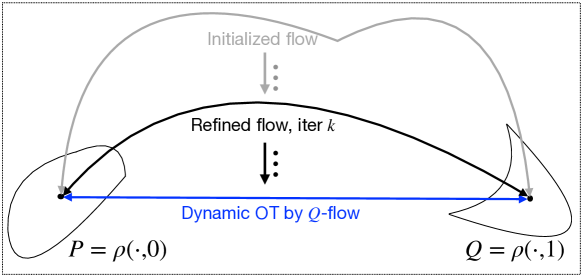
Figure 1: Illustration of learning the dynamic OT using our Q-flow (blue), which invertibly transports between $P$ and $Q$ over the interval $[0,1]$ with the least transport cost. Taking any initial flow (grey) between $P$ and $Q$, we iteratively refine flow trajectories to obtain flows with smaller transport costs (black), converging gradually to the dynamic OT between these two distributions.

3 Learning dynamic OT by Q-flow network

We introduce the formulation and training objective of the proposed OT Q-flow net in Section 3.1. The training technique consists of the end-to-end training (Section 3.2) and constructing the initial flow (Section 3.3).

3.1 Formulation and training objective

Given two sets of samples $\boldsymbol{X}=\{X_{i}\}_{i=1}^{N}$ and $\boldsymbol{\tilde{X}}=\{\tilde{X}_{j}\}_{j=1}^{M}$, where $X_{i}\sim P$ and $\tilde{X}_{j}\sim Q$ i.i.d., we train a neural ODE model $f(x,t;\theta)$ (1) to represent the transport map $T_{t}$. The formulation is symmetric from $P$ to $Q$ and vice versa, and the loss will also have two symmetrical parts. We call $P\rightarrow Q$ the forward direction and $Q\rightarrow P$ the reverse direction.

Our training objective is based on the dynamic OT (2) on time $[0,1]$, where we solve the velocity field $v(x,t)$ by $f(x,t;\theta)$. The terminal condition $\rho(\cdot,1)=q$ is relaxed by a KL divergence (see, e.g., (Ruthotto et al., 2020)). The training loss in the forward direction is written as

$$\mathcal{L}^{P\rightarrow Q}(\theta)=\mathcal{L}_{\rm KL}^{P\rightarrow Q}(\theta)+\gamma\mathcal{L}_{T}^{P\rightarrow Q}(\theta),$$ (3)

where $\mathcal{L}_{\rm KL}$ represents the relaxed terminal condition and $\mathcal{L}_{T}$ is the Wasserstein-2 transport cost to be specified below; $\gamma>0$ is a weight parameter, and with small $\gamma$ the terminal condition is enforced. Minimizing (3) over $\theta$ thus directly approximates the dynamic OT solution of (2), and we explore alternative training approaches in Appendix A.

KL loss.

Now we specify the first term in the loss (3) $\mathcal{L}_{\rm KL}^{P\rightarrow Q}$. We define the solution mapping of (1) from $s$ to $t$ as

$$T_{s}^{t}(x;\theta)=x(s)+\int_{s}^{t}f(x(t^{\prime}),t^{\prime};\theta)dt^{\prime},$$ (4)

which is also parameterized by $\theta$, and we may omit the dependence below. By the continuity equation in (2), $\rho(\cdot,t)=(T_{0}^{t})_{\#}p$. The terminal condition $\rho(\cdot,1)=q$ is relaxed by minimizing

$${\rm KL}(p_{1}||q)=\mathbb{E}_{x\sim p_{1}}\log(p_{1}(x)/q(x)),\quad p_{1}:=(T_{0}^{1})_{\#}p.$$

The expectation $\mathbb{E}_{x\sim p_{1}}$ is estimated by the sample average over $(X_{1})_{i}$ which observes density $p_{1}$ i.i.d., where $(X_{1})_{i}:=T_{0}^{1}(X_{i})$ is computed by integrating the neural ODE from time 0 to 1.

It remains to have an estimator of $\log(p_{1}/q)$ to compute ${\rm KL}(p_{1}||q)$. We propose to train a logistic classification network $c_{1}(x;\varphi_{c}):\mathbb{R}^{d}\rightarrow\mathbb{R}$ with parameters $\varphi_{c}$, which resembles the training of discriminators in GAN (Goodfellow et al., 2014). The inner-loop training of $c_{1}$ is by

$$\min_{\varphi_{c}}\frac{1}{N}\sum_{i=1}^{N}\log(1+e^{c_{1}(T_{0}^{1}(X_{i};\theta);\varphi_{c})})+\frac{1}{M}\sum_{j=1}^{M}\log(1+e^{-c_{1}(\widetilde{X}_{j};\varphi_{c})}).$$ (5)

The functional optimal $c_{1}^{*}$ of the population version of loss (5) equals $\log(q/p_{1})$ by direct computation, and as a result, ${\rm KL}(p_{1}||q)=-\mathbb{E}_{x\sim p_{1}}c_{1}^{*}(x)$. Now take the trained classification network $c_{1}$ with parameter $\hat{\varphi}_{c}$, we can estimate the finite sample KL loss as

$$\mathcal{L}_{\rm KL}^{P\rightarrow Q}(\theta)=-\frac{1}{N}\sum_{i=1}^{N}c_{1}(T_{0}^{1}(X_{i};\theta);\hat{\varphi}_{c}),$$ (6)

where $\hat{\varphi}_{c}$ is the computed minimizer of (5) solved by inner loops. In practice, when the density $p_{1}$ is close to $q$, the DRE by training classification net $c_{1}$ can be efficient and accurate. We will apply the minimization (5) after the flow net is properly initialized which guarantees the closeness of $p_{1}=(T_{0}^{1})_{\#}p$ and $q$ to begin with.

$W_{2}$ regularization.

Now we specify the second term in the loss (3) that defines the Wasserstein-2 regularization. To compute the transport cost $\mathcal{T}$ in (2) with velocity field $f(x,t;\theta)$, we use a time grid on $[0,1]$ as $0=t_{0}<t_{1}<\ldots<t_{K}=1$. The choice of the time grid is algorithmic (since the flow model is parameterized by $\theta$ throughout time) and may vary over experiments, see more details in Section 3.2. Define $h_{k}=t_{k}-t_{k-1}$, and $X_{i}(t;\theta):=T_{0}^{t}(X_{i};\theta)$, the $W_{2}$ regularization is written as

$$\mathcal{L}_{T}^{P\rightarrow Q}(\theta)=\sum_{k=1}^{K}\frac{1}{h_{k}}\left(\frac{1}{N}\sum_{i=1}^{N}\|X_{i}(t_{k};\theta)-X_{i}(t_{k-1};\theta)\|^{2}\right).$$ (7)

It can be viewed as a time discretization of $\mathcal{T}$. Meanwhile, since (omitting dependence on $\theta$) $X_{i}(t_{k})-X_{i}(t_{k-1})=T_{t_{k-1}}^{t_{k}}(X_{i}(t_{k-1}))$, the population form of (7) $\sum_{k=1}^{K}\mathbb{E}_{x\sim\rho(\cdot,t_{k-1})}\|T_{t_{k-1}}^{t_{k}}(x;\theta)\|^{2}/h_{k}$ in minimization can be interpreted as the discrete-time summed (square) Wasserstein-2 distance (Xu et al., 2022) $\sum_{k=1}^{K}{W_{2}(\rho(\cdot,t_{k-1}),\rho(\cdot,t_{k}))^{2}}/h_{k}.$ The $W_{2}$ regularization encourages a smooth flow from $P$ to $Q$ with a small transport cost, which also guarantees the invertibility of the model in practice when the trained neural network flow approximates the optimal flow in (2).

Training in both directions.

The formulation in the reverse direction is similar, where we transport $Q$-samples $\tilde{X}_{i}$ from 1 to 0 using the same neural ODE integrated in reverse time. Specifically, $\mathcal{L}^{Q\rightarrow P}(\theta)=\mathcal{L}_{\rm KL}^{Q\rightarrow P}(\theta)+\gamma\mathcal{L}_{T}^{Q\rightarrow P}(\theta)$, and $\mathcal{L}_{\rm{KL}}^{Q\rightarrow P}(\theta)=-\frac{1}{M}\sum_{j=1}^{M}\tilde{c}_{0}(T_{1}^{0}(\tilde{X}_{j};\theta);\hat{\varphi}_{\tilde{c}})$, where $\hat{\varphi}_{\tilde{c}}$ is obtained by inner-loop training of another classification net $\tilde{c}_{0}(x,\varphi_{\tilde{c}})$ with parameters $\varphi_{\tilde{c}}$ via

$$\min_{\varphi_{\tilde{c}}}\frac{1}{M}\sum_{j=1}^{M}\log(1+e^{\tilde{c}_{0}(T_{1}^{0}(\tilde{X}_{j};\theta);\varphi_{\tilde{c}})})+\frac{1}{N}\sum_{i=1}^{N}\log(1+e^{-\tilde{c}_{0}({X}_{i};\varphi_{\tilde{c}})}).$$ (8)

Define $\tilde{X}_{j}(t;\theta):=T_{1}^{t}(\tilde{X_{j}};\theta)$, the reverse-time $W_{2}$ regularization is

$$\mathcal{L}_{T}^{Q\rightarrow P}(\theta)=\sum_{k=1}^{K}\frac{1}{h_{k}}\left(\frac{1}{M}\sum_{j=1}^{M}\|\tilde{X}_{j}(t_{k-1};\theta)-\tilde{X}_{j}(t_{k};\theta)\|^{2}\right).$$

3.2 End-to-end training algorithm

In the end-to-end training, we assume that the Q-flow net has already been initiated as an approximate solution of the desired Q-flow, see more in Section 3.3. We then minimize $\mathcal{L}^{P\rightarrow Q}$ and $\mathcal{L}^{Q\rightarrow P}$ in an alternative fashion per “Iter”, and the procedure is given in Algorithm 1. Hyperparameter choices and sensitivity are further detailed in Appendix C.

Algorithm 1 OT Q-flow refinement

0:  Pre-trained initial flow network $f(x(t),t;\theta)$; training data $\boldsymbol{X}\sim P$ and $\boldsymbol{\widetilde{X}}\sim Q$; hyperparameters: $\{\gamma,\{t_{k}\}_{k=1}^{K},\texttt{Tot},E,E_{0},E_{\rm in}\}$.

0:  Refined flow network $f(x(t),t;\theta)$

1:  for Iter = $1,\ldots,\texttt{Tot}$ do

2:     (If Iter = 1) Train $c_{1}$ by minimizing (5) for $E_{0}$ epochs.

3:     for epoch = $1,\ldots,E$ do {$\triangleright$ $P\rightarrow Q$ refinement}

4:        Update $\theta$ of $f(x(t),t;\theta)$ by minimizing $\mathcal{L}^{P\rightarrow Q}$.

5:        Update $c_{1}$ by minimizing (5) for $E_{\rm in}$ epochs.

6:     end for

7:     (If Iter = 1) Train $\widetilde{c}_{0}$ by minimizing (8) for $E_{0}$ epochs.

8:     for epoch = $1,\ldots,E$ do {$\triangleright$ $Q\rightarrow P$ refinement}

9:        Update $\theta$ of $f(x(t),t;\theta)$ by minimizing $\mathcal{L}^{Q\rightarrow P}$.

10:        Update $\widetilde{c}_{0}$ by minimizing (8) for $E_{\rm in}$ epochs.

11:     end for

12:  end for

Time integration of flow.

In the losses (6) and (7), one need to compute the transported samples $X_{i}(t;\theta)$ and $\tilde{X}_{j}(t;\theta)$ on time grid points $\{t_{k}\}_{k=0}^{K}$. This calls for integrating the neural ODE on $[0,1]$, which we conduct on a fine time grid $t_{k,s}$, $s=0,\dots,S$, that divides each subinterval $[t_{k-1},t_{k}]$ into $S$ mini-intervals. We compute the time integration of $f(x,t;\theta)$ using a fixed-grid four-stage Runge-Kutta method on each mini-interval. The fine grid is used to ensure the numerical accuracy of ODE integration and the numerical invertibility of the Q-flow net, i.e., the error of using reverse-time integration as the inverse map (see inversion errors in Table A.1). It is also possible to first train the flow $f(x,t;\theta)$ on a time grid to warm start the later training on a refined grid, so as to improve convergence. We also find that the $W_{2}$ regularization can be computed at a coarser grid $t_{k}$ ($S$ is usually 3-5 in our experiments) without losing the effectiveness of Wasserstein-2 regularization. Finally, one can adopt an adaptive time grid, e.g., by enforcing equal $W_{2}$ movement on each subinterval $[t_{k-1},t_{k}]$ Xu et al. (2023), so that the representative points are more evenly distributed along the flow trajectory and the learning of the flow model can be further improved.

Inner-loop training of $c_{1}$ and $\tilde{c}_{0}$.

Suppose the flow net has been successfully warm-started, the transported distributions $(T_{0}^{1})_{\#}P\approx Q$ and $(T_{1}^{0})_{\#}Q\approx P$. The two classification nets are first trained for $E_{0}$ epochs before the loops of training the flow model and then updated for $E_{\rm in}$ inner-loop epochs in each outer-loop iteration. We empirically find that the diligent updates of $c_{1}$ and $\widetilde{c}_{0}$ in lines 5 and 10 of Algorithm 1 are crucial for successful end-to-end training of Q-flow net. As we update the flow model $f(x,t;\theta)$, the push-forwarded distributions $(T_{0}^{1})_{\#}P$ and $(T_{1}^{0})_{\#}Q$ are consequently changed. Then one will need to retrain $c_{1}$ and $\widetilde{c}_{0}$ timely to ensure an accurate estimate of the log-density ratio and consequently the KL loss. Compared with training the flow parameter $\theta$, the computational cost of the two classification nets is light which allows potentially a large number of inner-loop iterations if needed.

Computational complexity.

We measure the computational complexity by the number of function evaluations of $f(x(t),t;\theta)$ and of the classification nets $\{c_{1},\widetilde{c}_{0}\}$. Suppose the total number of epochs in outer loop training is $O(E)$; the dominating computational cost lies in the neural ODE integration, which takes ${O}(8KS\cdot E(M+N))$ function evaluations of $f(x,t;\theta)$. We remark that the Wasserstein-2 regularization (7) incurs no extra computation, since the samples $X_{i}(t_{k};\theta)$ and $\tilde{X}_{j}(t_{k};\theta)$ are available when computing the forward and reverse time integration of $f(x,t;\theta)$. The training of the two classification nets $c_{1}$ and $\widetilde{c}_{0}$ takes ${O}(4(E_{0}+EE_{\rm in})(M+N))$ additional evaluations of the two network functions since the samples $X_{i}(1;\theta)$ and $\tilde{X}_{j}(0;\theta)$ are already computed.

3.3 Flow initialization

We propose to initialize the Q-flow net by a flow model that approximately matches the transported distributions with the target distributions in both directions (and may not necessarily minimize the transport cost). Such an initialization will significantly accelerate the convergence of the end-to-end training, which can be viewed as a refinement of the initial flow.

The initial flow $f(x,t;\theta)$ may be specified using prior knowledge of the problem is available. Generally, when only two data sets $\boldsymbol{X},\boldsymbol{\tilde{X}}$ are given, the initial flow can be obtained by adopting existing methods in generative flows. In this work, we adopt two approaches: The first method is to construct the initial flow as a concatenation of two CNF models, each of which flows invertibly between $P$ and $Z$ and $Z$ and $Q$ for $Z\sim\mathcal{N}(0,I_{d})$. Any existing neural-ODE CNF models may be adopted for this initialization (Grathwohl et al., 2019; Xu et al., 2023). The second method adapts distribution interpolant neural networks. Specifically, one can use the linear interpolant mapping in (Rhodes et al., 2020; Choi et al., 2022; Albergo and Vanden-Eijnden, 2023) (see Appendix D), and train the neural network velocity field $f(x,t;\theta)$ to match the interpolation (Albergo and Vanden-Eijnden, 2023). Note that any other initialization scheme is compatible with the proposed end-to-end training of the Q-flow model to obtain the OT flow.

4 Infinitesimal density ratio estimation (DRE)

As has been shown in Rhodes et al. (2020); Choi et al. (2022), an interpolated sequence of distributions from $P$ to $Q$ can be used for the DRE of estimating $\log(q(x)/p(x))$ (reviewed in more detail in Appendix B), which is a fundamental task in statistical inference. Following the same idea, we propose to train an additional continuous-time neural network, called flow-ratio net, by minimizing a classification loss to distinguish distributions on neighboring time stamps along the trained Q-flow net trajectory. We will show in Section 5.1 that using the OT trajectory provided by the trained Q-flow net can benefit the accuracy of DRE.

Let $p(x,t)=(T_{t})_{\#}p$ and $T_{t}$ is the transport induced by the trained Q-flow net. Using (A.3), we propose to parametrize the time score ${\partial_{t}}\log p(x,t)$ by a neural network $r(x,t;\theta_{r})$ with parameter $\theta_{r}$, called the flow-ratio net. The training is by logistic classification applied to transported data distributions on consecutive time grid points: Given a deterministic time grid $0=t_{0}<t_{1}<\ldots<t_{L}=1$ (which again is an algorithmic choice; see Section B.3), we expect that the integral

$$R_{k}(x;\theta_{r}): =\int_{t_{k-1}}^{t_{k}}r(x,t;\theta_{r})dt\approx\int_{t_{k-1}}^{t_{k}}\partial_{t}\log p(x,t)dt$$

$$=\log(p(x,t_{k})/p(x,t_{k-1})).$$ (9)

By that, logistic classification recovers the log density ratio as has been used in Section 3.1, this suggests the loss on interval $[t_{k-1},t_{k}]$ as follows, where $X_{i}(t):=T_{0}^{t}(X_{i})$ and $T_{0}^{t}$ is computed by integrating the trained Q-flow net,

$$L_{k}^{P\rightarrow Q}(\theta_{r})=\frac{1}{N}\sum_{i=1}^{N}\log(1+e^{R_{k}(X_{i}(t_{k-1});\theta_{r})})+\frac{1}{N}\sum_{i=1}^{N}\log(1+e^{-R_{k}(X_{i}(t_{k});\theta_{r})}).$$ (10)

When $k=L$, the distribution of $X_{i}(t_{L})$ may slightly differ from that of $Q$ due to the error in matching the terminal densities in Q-flow net. Thus, replacing the 2nd term in (10) with an empirical average over the $Q$-samples $\tilde{X}_{j}$ may be beneficial. In the reverse direction, define $\tilde{X}_{j}(t):=T_{1}^{t}(\tilde{X}_{j})$, we similarly have $L_{k}^{Q\rightarrow P}(\theta_{r})=\frac{1}{M}\sum_{j=1}^{M}\log(1+e^{R_{k}(\tilde{X}_{j}(t_{k-1});\theta_{r})})+\frac{1}{M}\sum_{j=1}^{M}\log(1+e^{-R_{k}(\tilde{X}_{j}(t_{k});\theta_{r})})$, and when $k=1$, we replace the 1st term with an empirical average over the $P$-samples $X_{i}$. The training of the flow-ratio net is by

$$\min_{\theta_{r}}\sum_{k=1}^{L}{L}_{k}^{P\rightarrow Q}(\theta_{r})+{L}_{k}^{Q\rightarrow P}(\theta_{r}).$$ (11)

When trained successfully, the integral of $r(x,t;\theta_{r})$ over $t\in[0,1]$ yields the desired log density ratio $\log(q/p)$ by (A.3), and further the integral $\int_{s}^{t}r(x,t^{\prime};\theta_{r})dt^{\prime}$ provides an estimate of $\log(p(x,t)/p(x,s))$ for any $s<t$ on $[0,1]$. The details of minimizing (11) are given in Algorithm A.2.

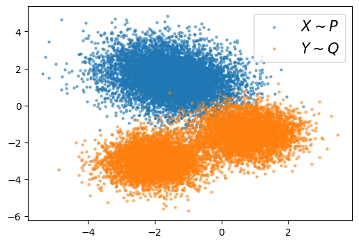
a Samples

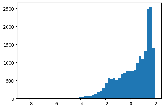
b MAE,Ours: 2.38

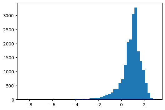
c DRE-$\infty$: 3.22

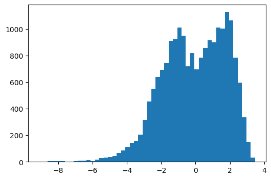
d TRE: 3.05

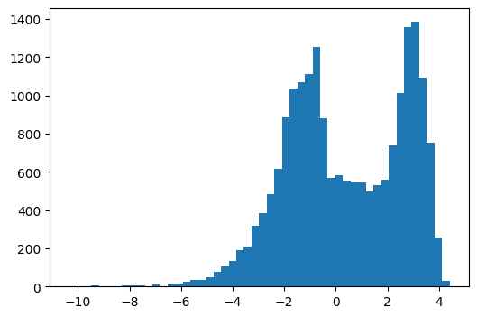
e 1 ratio: 8.20

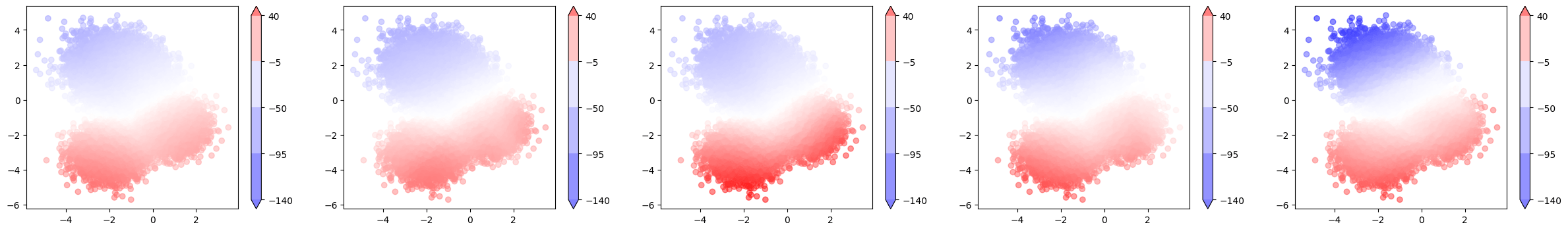
f Left to right: True ratio $r(x)$, $\hat{r}(x)$ by Ours, DRE-$\infty$, TRE, and 1 ratio.

Figure 2: Estimated log density ratio between 2D Gaussian mixture distributions $P$ (three components) and $Q$ (two components). Top: (a) training samples from $P$ and $Q$. (b)-(d) histograms of errors $\log(|r(x)-\hat{r}(x)|)$ computed at 10K test samples shown in log-scale. The MAE (A.4) are shown in the captions. Bottom: true and estimated $\log(q/p)$ from different models shown under shared color bars.

5 Experiments

In this section, we demonstrate the effectiveness of the proposed method on several downstream tasks. The benefits of using our dynamic OT map to improve DRE between $P$ and $Q$ are shown in Section 5.1. The comparison with popular OT baselines is shown in Section 5.2. The application to image-to-image translation is presented in Section 5.3. Code can be found at https://github.com/hamrel-cxu/FlowOT.

5.1 High-dimensional density ratio estimation (DRE)

We show the benefits of our flow-ratio net proposed in Section 4 on various DRE tasks, where flow-ratio net leverages the flow trajectory of a trained Q-flow net. In the experiments below, we denote our method as “Ours”, and compare against three baselines of DRE in high dimensions. The baseline methods are: 1 ratio (by training a single classification network using samples from $P$ and $Q$), TRE (Rhodes et al., 2020), and DRE-$\infty$ (Choi et al., 2022). We denote $P_{t_{k}}$ with density $p(\cdot,t_{k})$ as the pushforward distribution of $P$ by the Q-flow transport over the interval $[0,t_{k}]$. The set of distributions $\{P_{t_{k}}\}$ for $k=1,\ldots,L$ builds a bridge between $P$ and $Q$.

5.1.1 Toy data in 2d

a Trajectory from $P$ to $Q$

b Estimated $\log$-ratio between $P_{t_{k-1}}$ and $P_{t_{k}}$ by the trained flow-ratio net.

Figure 3: Q-flow trajectory between arbitrary 2D distributions and corresponding $\log$-ratio estimation. Top: intermediate distributions by Q-flow net. Bottom: corresponding $\log$-ratio estimated by flow-ratio net. Blue color indicates smaller estimates of the difference $\log(p(x,t_{k})/p(x,t_{k-1}))$ evaluated at the common support of the neighboring densities.

Gaussian mixtures.

We simulate $P$ and $Q$ as two Gaussian mixture models with three and two components, respectively, see additional details in Appendix C.1.1. We compute ratio estimates $\hat{r}(x)$ with the true value $r(x)$, which can be computed using the analytic expressions of the densities. The results are shown in Figure 2. We see from the top panel that the mean absolute error (MAE) of Ours is evidently smaller than those of the baseline methods, and Ours also incurs a smaller maximum error $|\hat{r}-r|$ on test samples. This is consistent with the closest resemblance of Ours to the ground truth (first column) in the bottom panel. In comparison, DRE-$\infty$ tends to over-estimate $r(x)$ on the support of $Q$, while TRE and one ratio can severely under-estimate $r(x)$ on the support of $P$. As both the DRE-$\infty$ and TRE models use the linear interpolant scheme (A.9), the result suggests the benefit of using Q-flow trajectory for DRE.

Two-moon to and from checkerboard.

We design two densities in $\mathbb{R}^{2}$ where $P$ represents the shape of two moons, and $Q$ represents a checkerboard; see additional details in Appendix C.1.1. For this more challenging case, the linear interpolation scheme (A.9) creates a bridge between $P$ and $Q$ as shown in Figure A.6. The flow visually differs from the one obtained by the trained Q-flow net, as shown in Figure 3(a), and the latter is trained to minimize the transport cost. The result of flow-ratio net is shown in Figure 3(b). The corresponding density ratio estimates of $\log p(x,t_{k})-\log p(x,t_{k-1})$ visually reflect the actual differences in the two neighboring densities.

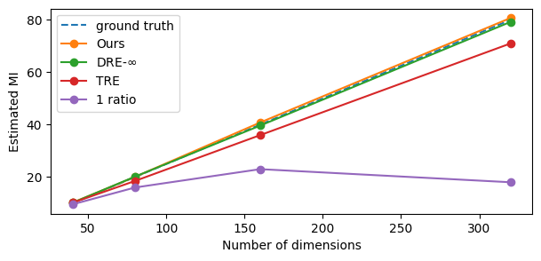
Figure 4: Estimated MI between two correlated high-dimensional Gaussian random variables.

5.1.2 Mutual Information estimation for high-dimensional data

We evaluate different methods of estimating the mutual information (MI) between two correlated random variables from given samples. In this example, we let $P$ and $Q$ be two high-dimensional Gaussian distributions following the setup in (Rhodes et al., 2020; Choi et al., 2022), where we vary the data dimension $d$ in the range of $\{40,80,160,320\}$. Additional details can be found in Appendix C.1.2.

Figure 4 shows the results by different methods, where the baselines are trained under their proposed default settings. We find that the estimated MI by our method almost perfectly aligns with the ground truth MI values, reaching nearly identical performance as DRE-$\infty$ does. Meanwhile, Ours outperforms the other two baselines, and the performance gaps increase as the dimension $d$ increases.

Table 1: DRE performance on the energy-based modeling task for MNIST, reported in BPD and lower, is better. Results for DRE-$\infty$ are from (Choi et al., 2022), and results for one ratio and TRE are from (Rhodes et al., 2020).

Choice of $Q$	RQ-NSF				Copula				Gaussian
Method	Ours	DRE-$\infty$	TRE	1 ratio	Ours	DRE-$\infty$	TRE	1 ratio	Ours	DRE-$\infty$	TRE	1 ratio
BPD ($\downarrow$)	1.05	1.09	1.09	1.09	1.14	1.21	1.24	1.33	1.31	1.33	1.39	1.96

5.1.3 Energy-based modeling of MNIST

We apply our approach in evaluating and improving an energy-base model (EBM) on the MNIST dataset (LeCun and Cortes, 2005). We follow the prior setup in (Rhodes et al., 2020; Choi et al., 2022), where $P$ is the empirical distribution of MNIST images, and $Q$ is the generated image distributions by three given pre-trained energy-based generative models: a Gaussian noise model, a Gaussian copula model, and a Rational Quadratic Neural Spline Flow model (RQ-NSF) (Durkan et al., 2019). The performance of DRE is measured using the “bits per dimension” (BPD) metric in (A.6). Additional details are in Appendix C.1.3.

The results show that Ours reaches the improved performance in Table 1 against baselines: it consistently reaches a smaller BPD than the baseline methods across all choices of $Q$. Meanwhile, we also note computational benefits in training: on one A100 GPU, Ours took approximately 8 hours to converge while DRE-$\infty$ took approximately 33 hours. In addition, we show the trajectory of improved samples from $Q$ to $\tilde{Q}$ for RQ-NSF using the trained Q-flow in Figure A.1. Figure A.2 in the appendix shows additional improved digits for all three specifications of $Q$.

5.2 Comparison with OT baselines

Table 2: OT benchmarks using Gaussian mixtures with increasing dimensions (columns). Metric values ($\mathcal{L}^{2}$-UVP, $\cos$) are shown in cells, with lower $\mathcal{L}^{2}$-UVP and higher $\cos$ being better. The last three rows are from (Korotin et al., 2021b) for comparisons.

Data dimension	32	64	128	256
Q-flow (Ours)	(3.27, 0.99)	(4.00, 0.98)	(2.12, 0.99)	(1.97, 0.99)
OTCFM (Tong et al., 2023)	(3.74, 0.99)	(4.64, 0.97)	(2.78, 0.99)	(3.02, 0.98)
MMv1 (Taghvaei and Jalali, 2019)	(6.9, 0.98)	(8.1, 0.97)	(2.2, 0.99)	(2.6, 0.99)
MMv2 (Fan et al., 2021)	(5.3, 0.99)	(10.1, 0.96)	(3.2, 0.99)	(2.7, 0.99)
W2 (Korotin et al., 2021c)	(6.0, 0.99)	(7.2, 0.97)	(2.0, 1.00)	(2.7, 1.00)

Table 3: OT benchmarks using CelebA64 images with different $P_{\text{Cpkt}}$ (columns). Metric values $\mathcal{L}^{2}$-UVP are in the left table (lower is better) and $\cos$ are in the right table (higher is better). The last three rows are from (Korotin et al., 2021b) for more comparisons.

Ckpt	Early	Mid	Late
Q-flow (Ours)	0.87	0.27	0.12
NOT (Korotin et al., 2023)	0.99	0.34	0.12
OTCFM (Tong et al., 2023)	1.2	0.39	0.16
W2 (Korotin et al., 2021c)	1.7	0.5	0.25
MM (Dam et al., 2019)	2.2	0.9	0.53
MM:R (Makkuva et al., 2020)	1.4	0.4	0.22

Cpkt	Early	Mid	Late
Q-flow (Ours)	0.99	0.97	0.97
NOT	0.99	0.96	0.96
OTCFM	0.99	0.96	0.95
W2	0.99	0.95	0.93
MM	0.98	0.90	0.87
MM:R	0.99	0.96	0.94

We compare our Q-flow with popular OT baselines on the OT benchmark (Korotin et al., 2021b). The goal is to match outputs from a trained OT map as closely as possible with those from the ground truth in the benchmark. Two metrics, $\mathcal{L}^{2}$-UVP in (A.7) and $\cos$ in (A.8), are used to evaluate performance, where lower $\mathcal{L}^{2}$-UVP and higher $\cos$ values indicate better performance. Details of the setup are provided in Appendix C.2.

High-dimensional Gaussian mixtures.

The goal is to transport between high-dimensional Gaussian mixtures optimally. We vary dimension $d\in\{32,64,128,256\}$, and in each dimension, the distribution $P$ is a mixture with three components, and $Q$ is a weighted average of two 10-component Gaussian mixtures. Table 2 shows that our Q-flow consistently reaches lower $\mathcal{L}^{2}$-UVP and higher or equal $\cos$ than OT baselines, indicating comparable or better performance on this example.

CelebA64 images.

The goal is to align CelebA64 faces (Liu et al., 2015) (denoted as $Q$) with faces generated by a pre-trained WGAN-QC (Liu et al., 2019) generator (denoted as $P_{\text{Cpkt}}$ for different checkpoints). In particular, three checkpoints of the WGAN-QC are considered (i.e., $\text{Cpkt}\in\{\text{Early, Mid, Late}\}$), where $P_{\text{Early}}$ contains generated faces that are the most blurry and faces from $P_{\text{Late}}$ are closest to true faces among the three. Quantitatively, results in Table 3 show that Q-flow outperforms other OT baselines. Figure A.3 in the appendix further shows high-quality faces as a result of using the trained Q-flow net on samples from $P_{\text{Cpkt}}$ for different Cpkt.

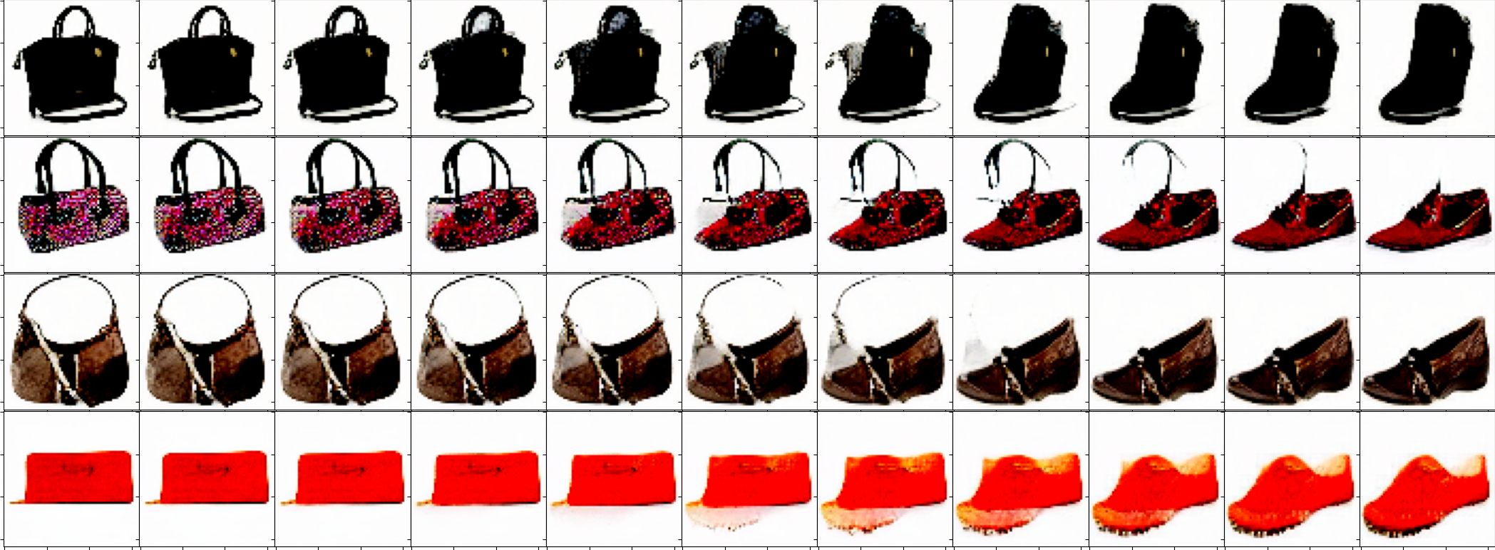
a Handbag $\rightarrow$ shoes

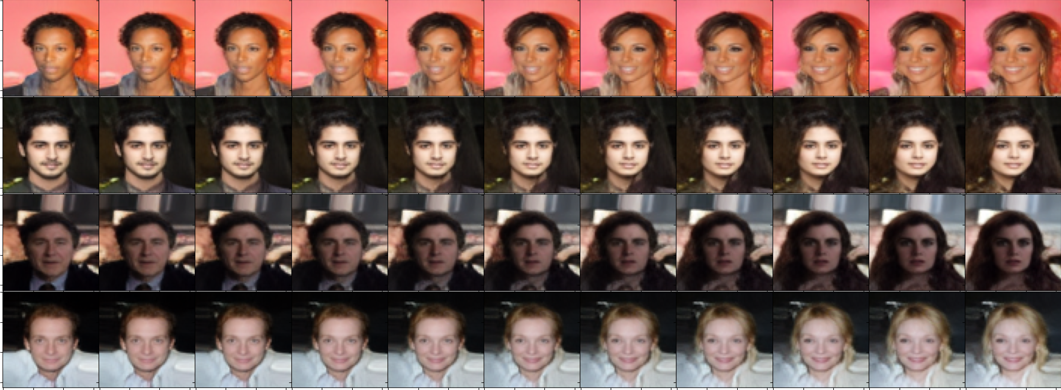
b CelebA male $\rightarrow$ female

Figure 5: Image-to-image translation: the trajectory of samples (in rows) from intermediate distributions of the Q-flow, as it pushes forward the base distribution (leftmost column) to the target distribution (rightmost column). Figure (a) shows the transition from handbag to shoe. Figure (b) shows the transition from CelebA male to female.

5.3 Image-to-image translation

We use Q-flow to learn the continuous-time OT between distributions of two sets of RGB images. The first set contains handbags (Zhu et al., 2016) and shoes (Yu and Grauman, 2014), and the second set contains CelebA male and female images. We denote handbags/males as $P$ and shoes/females as $Q$. We follow the setup in (Korotin et al., 2023), where the goal of the image-to-image translation task is to conditionally generate shoe/female images by mapping images of handbag/male through our trained Q-flow model. We train Q-flow in the latent space of a pre-trained variational auto-encoder (VAE) on $P$ and $Q$. Additional details are in Appendix C.3.

Figure 5 visualizes continuous trajectories from handbags/males to shoes/females generated by the Q-flow model. We find that Q-flow can capture the style and color nuances of corresponding handbags/males in the generated shoes/females as the flow model continuously transforms handbag/male images. Figure A.4 and A.5 in the appendix show additional generated shoes/females from handbags/males, respectively. Quantitatively, FIDs between generated and true images in the test set, as shown in Table 4 indicate Q-flow performs better than all three baselines. Meanwhile, as our Q-flow model learns a continuous transport map from source to target domains, it directly provides the gradual interpolation between source and target samples along the dynamic OT trajectory as shown in Figure 5.

Table 4: Image-to-image translation: FID comparison on the test sets. Lower FIDs are better. The baseline FIDs are quoted from (Korotin et al., 2023) for comparisons.

	Q-flow (ours)	Disco GAN (Kim et al., 2017)	Cycle GAN (Zhu et al., 2017)	NOT (Korotin et al., 2023)
Handbag $\rightarrow$ shoes	12.97	22.42	16.00	13.77
CelebA male $\rightarrow$ female	10.71	35.64	17.74	13.23

6 Discussion

In this work, we develop Q-flow neural-ODE model that smoothly and invertibly transports between a pair of arbitrary distributions $P$ and $Q$. The flow network is trained to find the dynamic optimal transport between the two distributions and is learned from finite samples from both distributions. The proposed flow model shows strong empirical performance on high-dimensional DRE, OT baselines, and image-to-image translation.

For future directions, first, the algorithm of training the Q-flow net can be further enhanced. Because the computational complexity scales with the number of time steps along the trajectory, more advanced time discretization schemes, like adaptive time grids, can further improve computational efficiency, which would be important for high dimensional problems. Second, there are many theoretical open questions, e.g., the theoretical guarantee of learning the OT trajectory, which goes beyond the scope of the current work. For the empirical results, extending to a broader class of applications and more real datasets will be useful.

Appendix A Alternative training schemes

One may modify the training loss (3) and develop alternative training schemes. The loss (3) is a time discretization of the BB equation (2), where the terminal condition $\rho(x,1)=q(x)$ is relaxed by minimizing the KL divergence. Hence, it is natural to consider other divergence measures as relaxation, such as the total variation, the Jensen–Shannon divergence, and so on. Developing efficient training algorithms based on such divergence measures is a promising future direction.

We take the maximum mean discrepancy (MMD) with the radial basis function (RBF) kernel as a concrete example. Given a RBF kernel $k(x,y)=\exp(-\|x-y\|^{2}/(2h^{2}))$ with bandwidth $h$, the squared population MMD between distributions $p$ and $q$ is

$$\text{MMD}(p,q)=\mathbb{E}_{x,x^{\prime}\sim p}[k(x,x^{\prime})]+\mathbb{E}_{y,y^{\prime}\sim q}[k(y,y^{\prime})]-2\mathbb{E}_{x\sim p,y\sim q}[k(x,y)].$$ (A.1)

Hence, one can replace the KL term $\mathcal{L}_{\rm KL}^{P\rightarrow Q}(\theta)$ in (6) by $\mathcal{L}_{\rm MMD}^{P\rightarrow Q}(\theta)$, which denotes the MMD between $p_{1}$ (the pushforward distribution of $p$ by the flow map $T_{0}^{1}(x;\theta)$) and $q$. In training, the population MMD in (A.1) would be approximated using mini-batch samples from $p$ and $q$.

We also note the pros and cons of using MMD vs. KL as relaxation techniques. Using MMD could be preferable because one does not need to parametrize a classification net $c(x)$ as in using KL, whose training also involves inner loop updates of $c(x)$. On the other hand, how to choose the kernel bandwidth and kernel functions are challenging problems for MMD to work well in high dimensions. Furthermore, the computation of MMD is $O(nm)$ on $n$ samples from $p$ and $m$ samples from $q$, unlike the $O(\max(n,m))$ linear rate when computing KL with $c(x)$.

Appendix B Infinitesimal density ratio estimation

We first introduce related works of DRE (Section B.1) and DRE preliminaries (Section B.2). We then present the complete algorithm for our proposed flow-ratio net in Section B.3.

B.1 DRE literature

Density ratio estimation between distributions $P$ and $Q$ is a fundamental problem in statistics and machine learning [Meng and Wong, 1996, Sugiyama et al., 2012, Choi et al., 2021]. It has direct applications in important fields such as importance sampling [Neal, 2001], change-point detection [Kawahara and Sugiyama, 2009], outlier detection [Kato and Teshima, 2021], mutual information estimation [Belghazi et al., 2018], etc. Various techniques have been developed, including probabilistic classification [Qin, 1998, Bickel et al., 2009], moment matching [Gretton et al., 2009], density matching [Sugiyama et al., 2008], etc. Deep NN models have been leveraged in classification approach Moustakides and Basioti [2019] due to their expressive power. However, as has been pointed out in [Rhodes et al., 2020], the estimation accuracy by a single classification may degrade when $P$ and $Q$ differ significantly.

To overcome this issue, [Rhodes et al., 2020] introduced a telescopic DRE approach by constructing intermediate distributions to bridge between $P$ and $Q$. [Choi et al., 2022] further proposed to train an infinitesimal, continuous-time ratio net via the so-called time score matching. Despite their improvement over the prior classification methods, both approaches rely on an unoptimal construction of the intermediate distributions between $P$ and $Q$. In contrast, our proposed Q-flow network leverages the expressiveness of deep networks to construct the intermediate distributions by the continuous-time flow transport, and the flow trajectory is regularized to minimize the transport cost in dynamic OT. The model empirically improves the DRE accuracy (see Section 5). In computation, [Choi et al., 2022] applies score matching to compute the infinitesimal change of log-density. The proposed flow-ratio net is based on classification loss training using a fixed time grid which avoids score matching and is computationally lighter (Section B.3).

B.2 Telescopic and infinitesimal DRE preliminaries

To circumvent the problem of DRE distinctly different $p$ and $q$, the telescopic DRE [Rhodes et al., 2020] proposes to “bridge” the two densities by a sequence of intermediate densities $p_{k}$, $k=0,\cdots,L$, where $p_{0}=p$ and $p_{L}=q$. The consecutive pairs of $(p_{k},p_{k+1})$ are chosen to be close so that the DRE can be computed more accurately, and then by

$$\log({q}(x)/{p}(x))=\log p_{L}(x)-\log p_{0}(x)=\sum_{k=0}^{L-1}\log p_{{k+1}}(x)-\log p_{k}(x),$$ (A.2)

the log-density ratio between $q$ and $p$ can be computed with improved accuracy than a one-step DRE. The infinitesmal DRE [Choi et al., 2022] considers a time continuity version of (A.2). Specifically, suppose the time-parameterized density $p(x,t)$ is differentiable on $t\in[0,1]$ with $p(x,0)=p$ and $p(x,1)=q$, then

$$\log(q(x)/p(x))=\log p(x,1)-\log p(x,0)=\int_{0}^{1}\partial_{t}\log p(x,t)dt.$$ (A.3)

The quantity ${\partial_{t}}\log p(x,t)$ was called the “time score” and can be parameterized by a neural network.

Algorithm A.2 Infinitesimal DRE training via flow-ratio net

0:  Training samples $\boldsymbol{X}\sim P$ and $\boldsymbol{\widetilde{X}}\sim Q$; pre-trained Q-flow net $f(x(t),t;\theta)$; hyperparameters: {$\{t_{k}\}_{k=1}^{L}$, Tot_iter}

0:  Trained network $r(x,t;\theta_{r})$.

1:  for $k=1,\ldots,L-1$ do

2:     Obtain $\{X_{i}(t_{k})\}_{i=1}^{N},\{\tilde{X}_{j}(t_{k})\}_{j=1}^{M}$ by transporting all training samples $\{\boldsymbol{X},\boldsymbol{\tilde{X}}\}$ using the given Q-flow net $f(x,t;\theta)$

3:  end for

4:  for Iter = $1,\ldots,\texttt{Tot\_iter}$ do

5:     Draw mini-batches of samples from $\{X_{i}(t_{k})\}_{i=1}^{N},\{\tilde{X}_{j}(t_{k})\}_{j=1}^{M}$.

6:     Train $\theta_{r}$ upon minimizing (11).

7:  end for

We use a trained Q-flow network $f(x,t;\theta)$ for infinitesimal DRE as a focused application.

B.3 Algorithm and computational complexity

Algorithm A.2 presents the complete flow-ratio algorithm. We use an evenly spaced time grid $t_{k}=k/L$ in all experiments. In practice, one can also progressively refine the time grid in training, starting from a coarse grid to train a flow-ratio net $r(x,t;\theta_{r})$ and use it as a warm start for training the network parameter $\theta_{r}$ on a refined grid. When the time grid is fixed, it allows us to compute the transported samples $\{X_{i}(t_{k})\}_{i=1}^{N},\{\tilde{X}_{j}(t_{k})\}_{j=1}^{M}$ on all $t_{k}$ once before the training loops of flow-ratio net (line 1-3). This part takes ${O}(8KS(M+N))$ function evaluations of the pre-trained Q-flow net $f(x,t;\theta)$. Suppose the training loops of lines 4-6 conduct $E$ epochs in total. Assume each time integral in $R_{k}$ (9) is computed by a fixed-grid four-stage Runge-Kutta method, then ${O}(4LE(M+N))$ function evaluations of $r(x,t;\theta_{r})$ is needed to compute the overall loss (11).

Appendix C Additional experimental details

When training all networks, we use the Adam optimizer [Kingma and Ba, 2015]. Unless otherwise specified, we start with an initial learning rate of 0.001.

C.1 High-dimensional density ratio estimation

C.1.1 Toy data in 2d

Gaussian mixtures.

Setup: We design the Gaussian mixtures $P$ and $Q$ as follows:

$$P=\frac{1}{3}\left(\mathcal{N}(\begin{bmatrix}-2\\ 2\end{bmatrix},0.75I_{2})+\mathcal{N}(\begin{bmatrix}-1.5\\ 1.5\end{bmatrix},0.25I_{2})+\mathcal{N}(\begin{bmatrix}-1\\ 1\end{bmatrix},0.75I_{2})\right)$$

$$Q=\frac{1}{2}\left(\mathcal{N}(\begin{bmatrix}0.75\\ -1.5\end{bmatrix},0.5I_{2})+\mathcal{N}(\begin{bmatrix}-2\\ -3\end{bmatrix},0.5I_{2})\right).$$

Then, 60K training samples and 10K test samples are randomly drawn from $P$ and $Q$. We intentionally designed the Gaussian mixtures so that their supports barely overlap. The goal is to estimate the $\log$-density ratio $r(x)=\log q(x)-\log p(x)$ on test samples.

Given a trained ratio estimator $\hat{r}(x)$, we measure its performance based on the MAE

$$\frac{1}{N^{\prime}}\sum_{i=1}^{N^{\prime}}|r(X_{i})-\hat{r}(X_{i})|+\frac{1}{M^{\prime}}\sum_{j=1}^{M^{\prime}}|r(\tilde{X}_{j})-\hat{r}(\tilde{X}_{j})|,$$ (A.4)

where we use $N^{\prime}$ and $M^{\prime}$ test samples from $P$ and $Q$, and $r(x)$ denotes the true density between $P$ and $Q$.

Q-flow : To initialize the two JKO-iFlow models that consists of the initial Q-flow , we specify the JKO-iFlow as:

• The flow network $f(x(t),t;\theta_{P})$ and $f(x(t),t;\theta_{Q})$ consists of fully-connected layers

  3$\rightarrow$128$\rightarrow$128$\rightarrow$2. The Softplus activation with $\beta=20$ is used. We concatenate $t$ along $x$ to form an augmented input into the network.

• We train the initial flow with a batch size of 2000 for 100 epochs along the grid

  $[0,0.25),[0.25,0.625),[0.625,1)$.

Table A.1: Inversion error $\mathbb{E}_{x\sim P}\|{T_{1}^{0}}({T_{0}^{1}}(x))-x\|^{2}_{2}+\mathbb{E}_{y\sim Q}\|{T_{0}^{1}}({T_{1}^{0}}(y))-y\|^{2}_{2}$ of Q-flow computed via sample average on the test split of the data set.

moon-to-checkerboard	High-dimensional Gaussians ($d=320$)	MNIST $(Q$ by RQ-NSF)
7.24e-7	3.44e-5	5.23e-5

To refine the Q-flow , we concatenate the trained $f(x(t),t;\theta_{P})$ and $f(x(t),t;\theta_{Q})$, where the former flows in $[0,1)$ to transport $P$ to $Z$ and the latter flows in $[1,0)$ to transport $Z$ to $Q$. We then use the time grid $[0,0.25),[0.25,0.625),[0.625,1),[1,0.625),[0.625,0.25),[0.25,0)$ to train $f(x(t),t;\theta)$ with $\theta=\{\theta_{P},\theta_{Q}\}$; we note that the above time grid can be re-scaled to obtain the time grid $\{t_{k}\}_{k=1}^{K}$ over $[0,1]$. The hyperparameters for Algorithm 1 are: Tot=2, $E_{0}=300$, $E=50$, $E_{\rm in}=4,\gamma=0.5$. The classification networks $\{c_{1},\widetilde{c}_{0}\}$ consists of fully-connected layers 2$\rightarrow$312$\rightarrow$312$\rightarrow$312$\rightarrow$1 with the Softplus activation with $\beta=20$, and it is trained with a batch of 200.

flow-ratio: The network consists of fully-connected layers 3$\rightarrow$256$\rightarrow$256$\rightarrow$256$\rightarrow$1 with the Softplus activation with $\beta=20$. The input dimension is 3 because we concatenate time $t$ along the input $x\in\mathbb{R}^{2}$ to form an augmented input. Using the trained Q-flow model, we then produce a bridge of 6 intermediate distributions using the pre-scaled grid $[0,0.25),[0.25,0.625),[0.625,1),$ $[1,0.625),[0.625,0.25),[0.25,0)$ for the Q-flow . We then train the network $r(x,t;\theta_{r})$ for 100 epochs with a batch size of 1000, corresponding to Tot_iter=6K in Algorithm A.2.

Two-moon to and from checkerboard.

Setup: We generate 2D samples whose marginal distribution has the shape of two moons and a checkerboard (see Figure 3(a), leftmost and rightmost scatter plots). We randomly sample 100K samples from $P$ and $Q$ to train the Q-flow and the infinitesimal DRE.

Q-flow : To initialize the two JKO-iFlow models that consists of the initial Q-flow , we specify the JKO-iFlow as:

• The flow network $f(x(t),t;\theta_{P})$ and $f(x(t),t;\theta_{Q})$ consists of fully-connected layers

  3$\rightarrow$256$\rightarrow$256$\rightarrow$2. The Softplus activation with $\beta=20$ is used. We concatenate $t$ along $x$ to form an augmented input into the network.

• We train the initial flow with a batch size of 2000 for 100 epochs along the grid

  $[0,0.25),[0.25,0.5),[0.5,0.75),$ $[0.75,1)$.

To refine the Q-flow , we concatenate the trained $f(x(t),t;\theta_{P})$ and $f(x(t),t;\theta_{Q})$, where the former flows in $[0,1]$ to transport $P$ to $Z$ and the latter flows in $[1,0]$ to transport $Z$ to $Q$. We then use the grid $[0,0.25),[0.25,0.5),[0.5,0.75),[0.75,1),[1,0.75),[0.75,0.5),[0.5,0.25),[0.25,0)$ (which can be re-scaled to form the time grid over $[0,1)$) to train $f(x(t),t;\theta)$ with $\theta=\{\theta_{P},\theta_{Q}\}$. The hyperparameters for Algorithm 1 are: Tot=2, $E_{0}=300$, $E=50$, $E_{\rm in}=4,\gamma=0.5$. The classification networks $\{c_{1},\widetilde{c}_{0}\}$ consists of fully-connected layers 2$\rightarrow$312$\rightarrow$312$\rightarrow$312$\rightarrow$1 with the Softplus activation with $\beta=20$, and it is trained with a batch of 200.

flow-ratio: The network consists of fully-connected layers 3$\rightarrow$256$\rightarrow$256$\rightarrow$256$\rightarrow$1 with the Softplus activation with $\beta=20$. The input dimension is three because we concatenate time $t$ along the input $x\in\mathbb{R}^{2}$ to form an augmented input. Using the trained Q-flow model, we then produce a bridge of 8 intermediate distributions using the pre-scaled grid interval $[0,0.25),[0.25,0.5),[0.5,0.75)$, $[0.75,1),[1,0.75),$ $[0.75,0.5),[0.5,0.25),[0.25,0)$ for the Q-flow . We then train the network $r(x,t;\theta_{r})$ for 500 epochs with a batch size of 500, corresponding to Tot_iter=100K in Algorithm A.2.

C.1.2 Mutual Information estimation for high-dimensional data

Setup: The task is to estimate the $\log$-density ratio between two high-dimensional Gaussian distributions of dimension $d$, where this task can be viewed as an MI estimation problem. We follow the same setup as in [Rhodes et al., 2020, Choi et al., 2022]. The first Gaussian distribution $P=\mathcal{N}(0,\Sigma)$, where $\Sigma$ is a block-diagonal covariance matrix with $2\times 2$ small blocks having one on the diagonal and 0.8 on the off-diagonal. The second Gaussian distribution $Q=\mathcal{N}(0,I_{d})$ is the isotropic Gaussian in $\mathbb{R}^{d}$. We randomly draw 100K samples for each choice of $d$, which varies from 40 to 320.

To be more precise, we hereby draw the connection of the DRE task with mutual information (MI) estimation, following [Rhodes et al., 2020]. We first recall the definition of MI between two correlated random variables $U$ and $V$:

$$I(U;V)=\mathbb{E}_{p(U,V)}\left[\log\frac{p(U,V)}{p(U)p(V)}\right].$$ (A.5)

Now, given $X=(x_{1},\ldots,x_{d})\sim P=\mathcal{N}(0,\Sigma)$, we define $U=(x_{1},x_{3},\ldots,x_{d-1})$ and $V=(x_{2},x_{4},\ldots,x_{d})$. By the construction of $\Sigma$, we thus have $p(U)p(V)=Q(X)$ for $Q=\mathcal{N}(0,I_{d})$. As a result, the MI in (A.5) between $U$ and $V$ is equivalent to $\mathbb{E}_{X\sim P}[-r(X)]$, where $r(x)=\log\frac{Q(x)}{P(x)}$ is the objective of interest in DRE.

Q-flow : We specify the following when training the Q-flow :

• The flow network $f(x(t),t;\theta)$ consists of fully-connected layers with dimensions

  (d+1)$\rightarrow$min(4d,1024)$\rightarrow$min(4d,1024)$\rightarrow$d. The Softplus activation with $\beta=20$ is used. We concatenate $t$ along $x$ to form an augmented input into each network layer.

• We train the flow network for 100 epochs with a batch size of 500, in both the flow initialization phase and the end-to-end refinement phase. The flow network is trained along the evenly-spaced time grid $[t_{k-1},t_{k})$ for $k=1,\ldots,L_{d}$, and we let $t_{k}=k/L_{d}$. $L_{d}$ increases as the dimension $d$ increases. We specify the choices as

  $(L_{d},d)\in\{(4,40),(6,80),(7,160),(8,320)\}$.

The hyperparameters for Algorithm 1 are: Tot=2, $E_{0}=500$, $E=100$, $E_{\rm in}=2,\gamma=0.5$. The classification networks $\{c_{1},\widetilde{c}_{0}\}$ consists of fully-connected layers $d\rightarrow\min(4d,1024)\rightarrow\min(4d,1024)$$\rightarrow\min(4d,1024)\rightarrow 1$ with the Softplus activation with $\beta=20$, and it is trained with a batch of 200.

flow-ratio: The network consists of fully-connected layers with dimensions

(d+1)$\rightarrow$min(4d,1024)$\rightarrow$min(4d,1024)$\rightarrow$min(4d,1024)$\rightarrow$1, using the Softplus activation with $\beta=20$. The input dimension is $d+1$ because we concatenate time $t$ along the input $x\in\mathbb{R}^{d}$ to form an augmented input. Using the trained Q-flow model, we then produce a bridge of $L_{d}$ intermediate distributions using the grid $[t_{k-1},t_{k})$ specified above for the Q-flow . We then train the network $r(x,t;\theta_{r})$ for 1000 epochs with a batch size of 512, corresponding to Tot_iter=195K in Algorithm A.2.

C.1.3 Energy-based modeling of MNIST

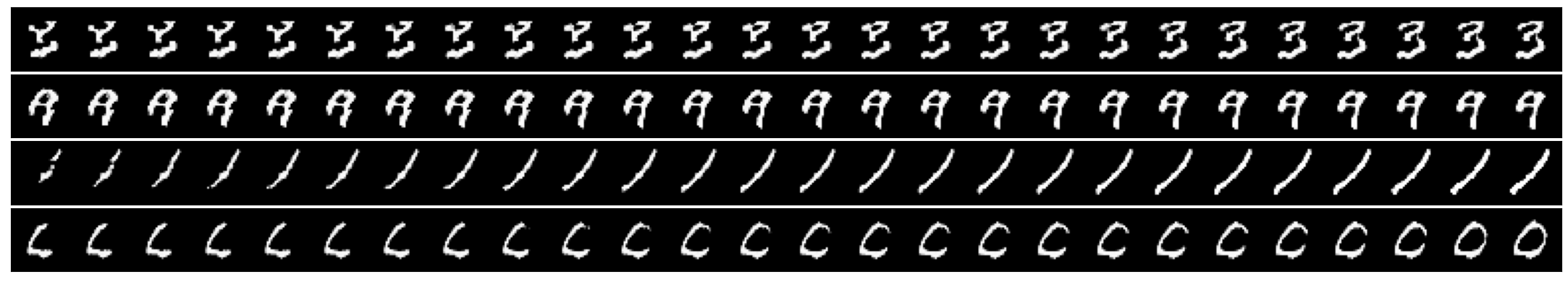
Figure A.1: The trajectory of samples (in rows) from intermediate distributions of the Q-flow, as it pushes forward the base distribution (leftmost column) to the target distribution (rightmost column). The figure shows the improvement of generated digits using the Q-flow.

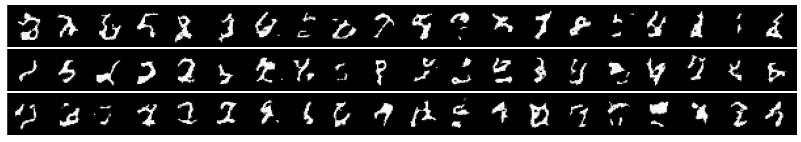
a RQ-NSF: raw samples from $Q$

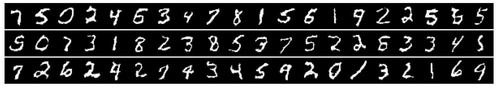
b RQ-NSF: improved samples from $\tilde{Q}$

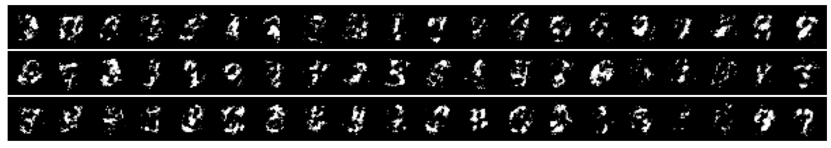
c Copula: raw samples from $Q$

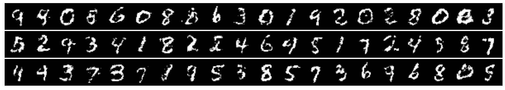
d Copula: improved samples from $\tilde{Q}$

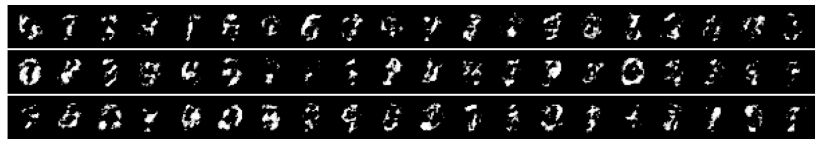
e Gaussian: raw samples from $Q$

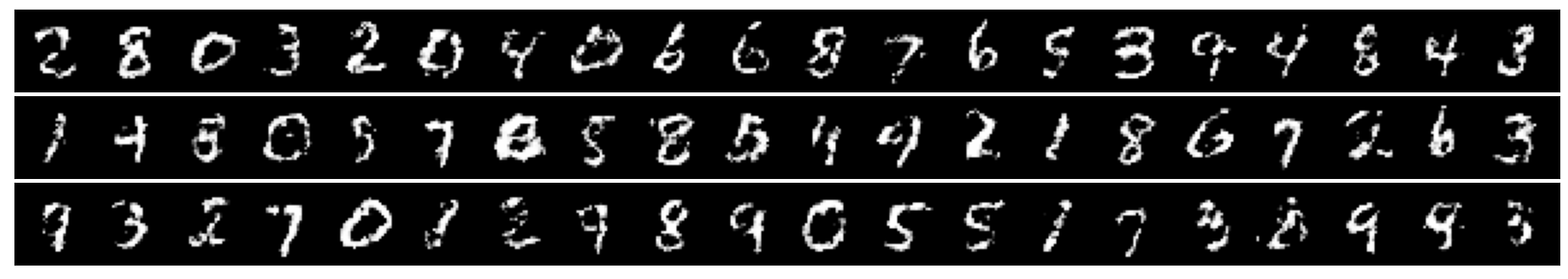
f Gaussian: improved samples from $\tilde{Q}$

Figure A.2: Improvement in generated samples from $Q$, where $Q$ is given by RQ-NSF, Copula, or Gaussian. Each of the three choices of $Q$ is defined by a pre-trained invertible model $F$ that yields $Q=F_{\#}\mathcal{N}(0,I_{d})$.

Setup. We discuss how each of the three $Q$ distributions is obtained based on [Rhodes et al., 2020, Choi et al., 2022] and how we apply Q-flow and flow-ratio nets to the problem. Specifically, the MNIST images are in dimension $d=28^{2}=784$, and each of the pre-trained models provides an invertible mapping $F:\mathbb{R}^{d}\to\mathbb{R}^{d}$, where $Q=F_{\#}\mathcal{N}(0,I_{d})$. We train a Q-flow net between $(F^{-1})_{\#}P$ and $(F^{-1})_{\#}Q$, the latter by construction equals $\mathcal{N}(0,I_{d})$. Using the trained Q-flow net, we go back to the input space and train the flow-ratio net using the intermediate distributions between $P$ and $Q$.

The trained flow-ratio $r(x,s;\hat{\theta}_{r})$ provides an estimate of the data density $p(x)$ by $\hat{p}(x)$ defined as $\log\hat{p}(x)=\log q(x)-\int_{0}^{1}r(x,s;\hat{\theta}_{r})ds$, where $\log q(x)$ is given by the change-of-variable formula using the pre-trained model $F$ and the analytic expression of $\mathcal{N}(0,I_{d})$. As a by-product, since our Q-flow net provides an invertible mapping $T_{0}^{1}$, we can use it to obtain an improved generative model on top of $F$. Specifically, the improved distribution $\tilde{Q}:=(F\circ T^{0}_{1})_{\#}\mathcal{N}(0,I_{d})$, that is, we first use Q-flow to transport $\mathcal{N}(0,I_{d})$ and then apply $F$. The performance of the improved generative model can be measured using the “bits per dimension” (BPD) metric:

$$\text{BPD}=\frac{1}{N^{\prime}}\sum_{i=1}^{N^{\prime}}[-\log\hat{p}(X_{i})/(d\log 2)],$$ (A.6)

where $X_{i}$ are $N^{\prime}$=10K test images drawn from $P$. BPD has been a widely used metric in evaluating the performance of generative models [Theis et al., 2015, Papamakarios et al., 2017]. In our setting, the BPD can also be used to compare the performance of the DRE.

Q-flow : We specify the following when training the Q-flow :

• The flow network $f(x(t),t;\theta)$ consists of fully-connected layers with dimensions

  (d+1)$\rightarrow$1024$\rightarrow$1024$\rightarrow$1024$\rightarrow$d. The Softplus activation with $\beta=20$ is used. We concatenate $t$ along $x$ to form an augmented input into the network.

• In a block-wise fashion, we train the network with a batch size of 1000 for 100 epochs along the grid $[t_{k-1},t_{k-1}+h_{k})$ for $k=1,\ldots,5$. We let $h_{k}=0.5\cdot 1.1^{k-1}$.

The hyperparameters for Algorithm 1 are: Tot=2, $E_{0}=100$, $E=500$, $E_{\rm in}=2,\gamma=0.5$. The classification networks $\{c_{1},\widetilde{c}_{0}\}$ consists of fully-connected layers $784\rightarrow 1024\rightarrow 1024$$\rightarrow 1024\rightarrow$1 with the Softplus activation with $\beta=20$, and it is trained with a batch of 200.

flow-ratio: We use the same convolutional U-Net as described in [Choi et al., 2022, Table 2], which consists of an encoding block and a decoding block comprised of convolutional layers with varying filter sizes. Using the trained Q-flow model, we then produce a bridge of 5 intermediate distributions using the intervals $[t_{k-1},t_{k-1}+h_{k})$ specified above for the Q-flow . We then train the network $r(x,t;\theta_{r})$ for 300 epochs with a batch size of 128, corresponding to Tot_iter=117K in Algorithm A.2.

C.2 Comparison with OT methods

We summarize the setup and comparison metrics based on [Korotin et al., 2021b]. To assess the quality of a trained transport map $\hat{T}:\mathbb{R}^{d}\rightarrow\mathbb{R}^{d}$ from $P$ to $Q$ against a ground truth $T^{*}:\mathbb{R}^{d}\rightarrow\mathbb{R}^{d}$, the authors use two metrics: unexplained variance percentage ($\mathcal{L}^{2}$-UVP) [Korotin et al., 2021a] and cosine similarity ($\cos$), which are defined as

$$\mathcal{L}^{2}\text{-UVP} =100\cdot\frac{\mathbb{E}_{x\sim P}\|\hat{T}(x)-T^{*}(x)\|_{2}^{2}}{\text{Var}(Q)}\%.$$ (A.7)

$$\cos =\frac{\mathbb{E}_{x\sim P}\left\langle\hat{T}(x)-x,T^{*}(x)-x\right\rangle_{\ell_{2}}}{\mathbb{E}_{x\sim P}\|\hat{T}(x)-x\|_{2}\cdot\mathbb{E}_{x\sim P}\|T^{*}(x)-x\|_{2}}.$$ (A.8)

The metrics are evaluated using $2^{14}$ random samples from $P$.

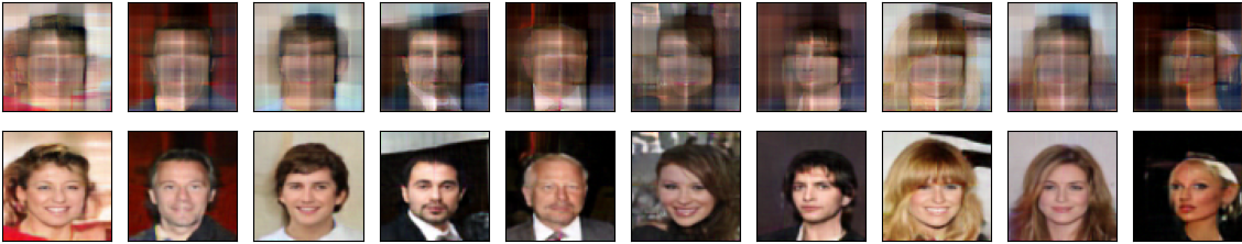
a Fitted Q-flow on $P_{\text{Early}}~{}(\text{top})\rightarrow Q~{}(\text{bottom})$.

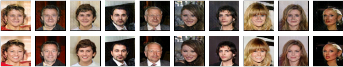
b Fitted Q-flow on $P_{\text{Mid}}~{}(\text{top})\rightarrow Q~{}(\text{bottom})$.

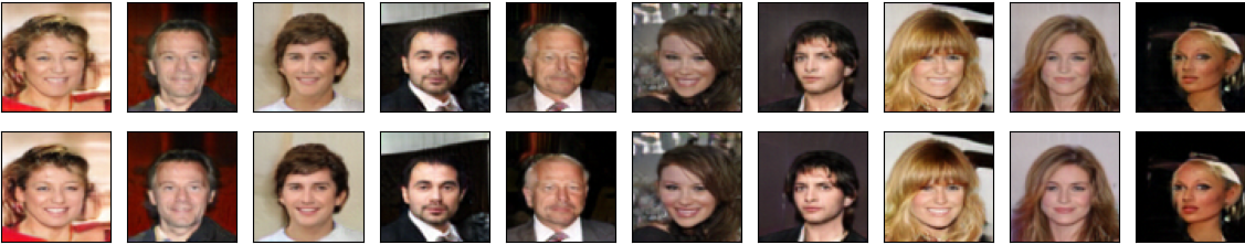
c Fitted Q-flow on $P_{\text{Late}}~{}(\text{top})\rightarrow Q~{}(\text{bottom})$.

Figure A.3: Fitted Q-flow between $P_{\text{Ckpt}}$ for $\text{Ckpt}\in\{\text{Early, Mid, Late}\}$ and $Q$. In each sub-figure, the first row contains random $x\sim P_{\text{Ckpt}}$ and the second row contains generated faces $T(x)$ using the trained Q-flow net $T$.

High-dimensional Gaussian mixtures.

In each dimension $d$, the distribution $P$ is a mixture of three Gaussians. The distribution $Q$ is constructed as follows: first, the authors construct two Gaussian mixtures $Q_{1}$ and $Q_{2}$ with 10 components. Then, they train approximate transport maps $\nabla\psi_{i}\#P\approx Q_{i}$, where $\psi_{i}$ is trained via [Korotin et al., 2021c]. The target $Q$ is obtained as $Q=\frac{1}{2}(\nabla\psi_{1}+\nabla\psi_{2})\#P$.

In Q-flow, the flow architecture $f(x(t),t;\theta)$ consists of fully connected layers of dimensions $2d-4d-8d-4d-2d$ with ReLU activation. The initialization of the flow is done by the method of Interflow Albergo and Vanden-Eijnden [2023], where at each step, we draw random batches of 2048 samples from $P$ and $Q$. We trained the initialized flow for 50K steps. To apply Algorithm 1, we let $\gamma=0.1$, $t_{k}=k/5$ for $k=0,\ldots,5$, and Tot=1. The classifiers $c_{1}$ and $\tilde{c}_{0}$ consist of fully-connected layers of dimensions $4d-4d-4d-4d$ with ReLU activation. These classifiers are initially trained for 10000 batches with batch size 2048. We train flow parameters $\theta$ for 10000 batches in every iteration with a batch size of 2048, and we update the training of $c_{1}$ and $\tilde{c}_{0}$ every 10 batches of training $\theta$ to train them for 10 inner-loop batches.

CelebA64 images [Liu et al., 2015]

The authors first fit 2 generative models using WGAN-QC [Liu et al., 2019] on the CelebA dataset. They then pick intermediate training checkpoints to product continuous measures $P^{k}_{\text{Early}},P^{k}_{\text{Mid}},P^{k}_{\text{Late}}$ for these 2 models ($k=1,2$). Then, for each $k\in\{1,2\}$ and $\text{Cpkt}\in\{\text{Early, Mid, Late}\}$, they use [Korotin et al., 2021c] to fit an approximate transport map $\nabla\psi^{k}_{\text{Ckpt}}$ such that $\nabla\psi^{k}_{\text{Ckpt}}\#Q\approx P^{k}_{\text{Ckpt}}$. The distributions $P_{\text{Ckpt}}$ are then obtained as $P_{\text{Ckpt}}=\frac{1}{2}(\nabla\psi^{1}_{\text{Ckpt}}+\nabla\psi^{2}_{\text{Ckpt}})\#Q.$

In Q-flow, the flow architecture $f(x(t),t;\theta)$ consists of convolutional layers of dimensions 64-128-128-256-256-512-512, followed by convolutional transpose layers whose filters mirror the convolutional layers. The kernel sizes are 3-4-3-4-3-4-3-3-4-3-4-3-4-3 with strides 1-2-1-2-1-2-1-1-2-1-2-1-2-1. We use the ReLU activation. The initialization of the flow is done by the method of Interflow Albergo and Vanden-Eijnden [2023] for 30K steps with 128 batch size. To apply Algorithm 1, we let $\gamma=1$, $t_{k}=k/3$ for $k=0,\ldots,3$, and Tot=1. The architecture of the classifier networks $c_{1}$ and $\tilde{c}_{0}$ are ResNets used in WGAN-QC [Liu et al., 2019]. These classifiers are initially trained for 5000 batches with batch size 128. We train flow parameters $\theta$ for 10000 batches in every iteration with a batch size of 128, and we update the training of $c_{1}$ and $\tilde{c}_{0}$ every 5 batches of training $\theta$ to train them for 1 inner-loop batch.

a Test handbag images from $P$

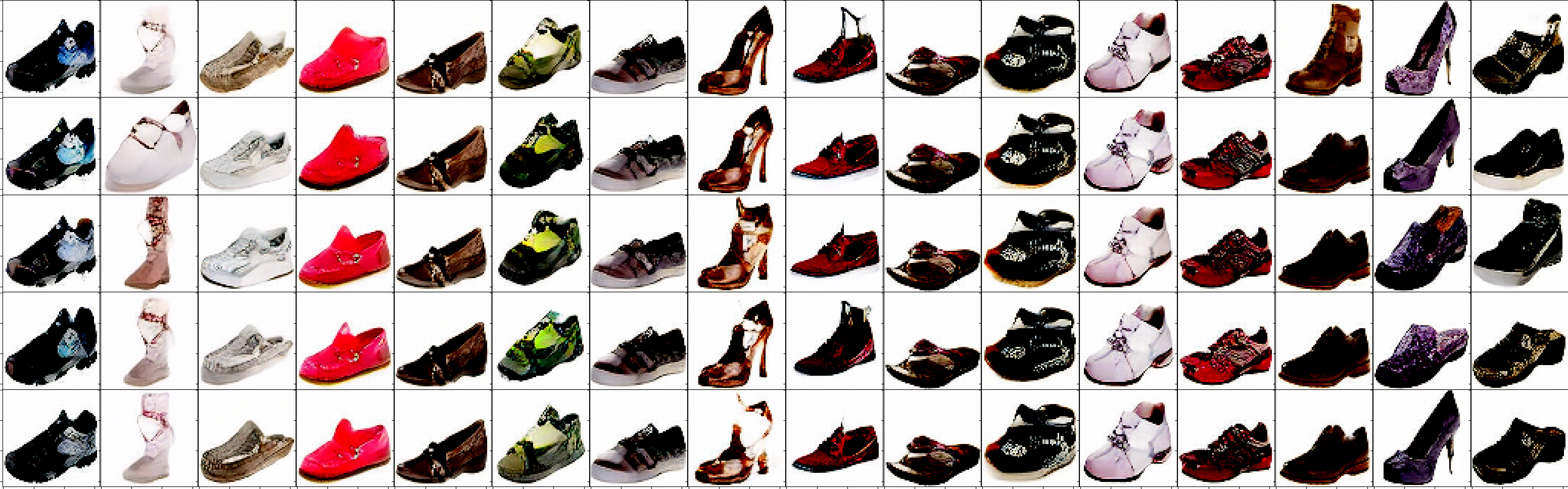
b Different generated shoe images by Q-flow model

Figure A.4: Additional test images of handbag (in true $P$, figure (a)) and corresponding generated shoe images by Q-flow model (in generated $Q$, figure (b)). To generate different shoes for a given handbag, we sample random latent codes given by the VAE, map them through the trained Q-flow model, and decode them back through the VAE decoder to visualize different generated shoes in the pixel space.

a Test male images from $P$

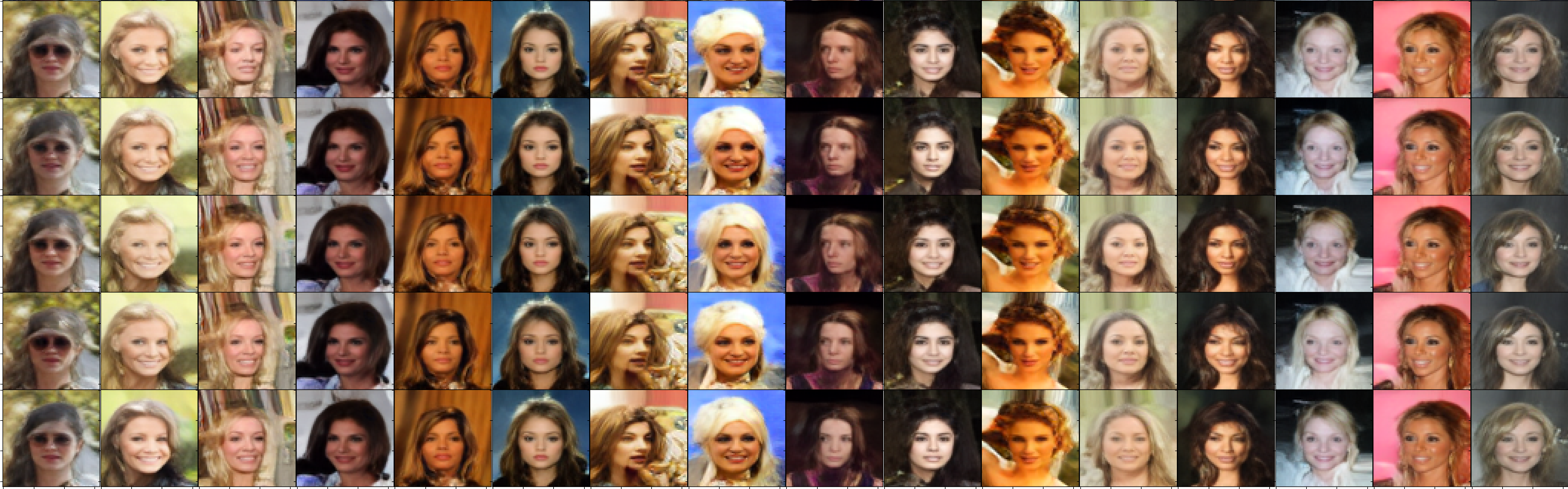
b Different generated female images by Q-flow model

Figure A.5: Additional test images of males (in true $P$, figure (a)) and corresponding generated female images by Q-flow model (in generated $Q$, figure (b)). To generate different females for a given male, we sample random latent codes given by the VAE, map them through trained Q-flow model, and decode back through the VAE decoder to visualize different generated females in the pixel space.

C.3 Image-to-image translation

The dataset of handbags $P$ has 137K images and the dataset of shoes $Q$ has 50K images, which are (3,64,64) RGB images. The dataset of CelebA males $P$ has 90K images and the dataset of CelebA females $Q$ has 110K images, which are (3,64,64) RBG images as well. Following [Korotin et al., 2023], we train on 90% of the total data from $P$ and $Q$ and reserve the rest 10% data as the test set. The FIDs are computed between generated shoe/female images (from the test handbag/male images) and true shoe/female images from the test set.

We first train a single deep VAE on both $P$ and $Q$. We train the deep VAE in an adversarial manner following [Esser et al., 2021]. Specifically, given a raw image input $X$, the encoder $\mathcal{E}$ of the VAE maps $X$ to $(\mu(X),\Sigma(X))$ parametrizing a multivariate Gaussian of dimension $d$. Then, the VAE is trained so that for a random latent code $X_{enc}\sim\mathcal{N}(\mu(X),\Sigma(X))$, the decoded image $\mathcal{D}(X_{enc})\approx X$. In our case, each latent code $X_{enc}$ has shape $(12,8,8)$, so that $d=768$.

The training data for Q-flow are thus sets of random latent codes $X_{enc}$ (obtained from $X\sim P$) and $Y_{enc}$ (obtained from $Y\sim P$), where Q-flow finds the dynamic OT between the marginal distributions of $X_{enc}$ and $Y_{enc}$. We then obtain the trajectory between $P$ and $Q$ by mapping the OT trajectory in latent space by the decoder $\mathcal{D}$

In Q-flow, the flow architecture $f(x(t),t;\theta)$ consists of convolutional layers of dimensions 12-64-256-512-512-1024, followed by convolutional transpose layers whose filters mirror the convolutional layers. The kernel sizes are 3-3-3-3-3-3-3-4-3-3 with strides 1-1-2-1-1-1-1-2-1-1. We use the softplus activation with $\beta=20$. The initialization of the flow is done by the method of Interflow Albergo and Vanden-Eijnden [2023], where at each step, we draw random batches of 128 $X$ and 128 $Y$ and then obtain 128 random latent codes $X_{enc}$ and 128 $Y_{enc}$. We trained the initialized flow for 26K steps on the bag-shoe example and for 15K steps on the male-female example. To apply Algorithm 1, we let $\gamma=0.05$ (bag-shoe) or $\gamma=0.1$ (male-female), $t_{k}=k/10$ for $k=0,\ldots,10$, and Tot=1. The architecture of the classifier networks $c_{1}$ and $\tilde{c}_{0}$ is based on [Choi et al., 2022], where the encoding layers of the classifier are convolutional filters of sizes 12-256-512-512-1024-1024 with kernel size equal to 3 and strides equal to 1-1-2-1-1. The decoding layers of the classifier resemble the encoding layers, and the final classification is made by passing the deep decoded feature through a fully connected network with size 768-768-768-1. These classifiers are initially trained for 4000 batches with batch size 512. We train flow parameters $\theta$ for 10000 batches (bag-shoe) or for 6000 batches (male-female) in every iteration with a batch size of 256, and we update the training of $c_{1}$ and $\tilde{c}_{0}$ every 10 batches of training $\theta$ to train them for 20 inner-loop batches.

C.4 Hyper-parameter sensitivity

Table A.2: BPD on MNIST with RQ-NSF target $Q$ over combinations of $\gamma$ in Algorithm 1 and time grid $\{t_{k}\}$ in Algorithm A.2.

$\gamma\ \&\ \{t_{k}\}$	$t_{k}=k/L$	$t_{k}=(k/L)^{2}$	$t_{k}=\sqrt{k/L}$
0.5	1.046	1.044	1.047
1	1.042	1.041	1.044
5	1.057	1.055	1.062

Overall, we did not purposely tune the hyperparameters in Section 5, and found that the Algorithm 1 and A.2 are not sensitive to hyper-parameter selections. We conduct additional ablation studies by varying the combination of $\gamma$ in Algorithm 1 and the time grid $\{t_{k}\}$ in Algorithm A.2. We tested all combinations on the MNIST example in Section 5.1.3 with RQ-NSF target $Q$. Table A.2 below presents our method’s performance, with the highest BPD (1.062) remaining lower than those by other DRE baselines in Table 1 (the lowest of which is 1.09). Small variations in the table can be attributed to the learned OT trajectory influenced by the choice of $\gamma$. Specifically, smaller $\gamma$ may lead to less smooth trajectories between $P$ and $Q$. In contrast, larger $\gamma$ may result in a higher KL-divergence between the pushed and target distributions due to insufficient amount of distribution transportation by the refined flow, both potentially impacting DRE accuracy.

Appendix D Linear stochastic interpolation used in Rhodes et al. [2020]

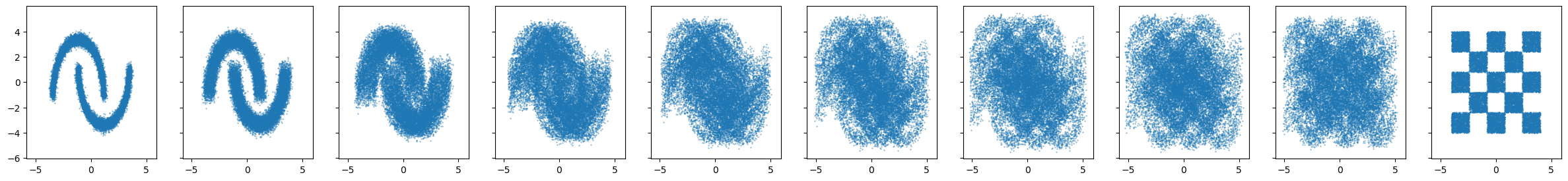
Figure A.6: Bridge construction between $P$ (leftmost) and $Q$ (rightmost) via the linear interpolation scheme (A.9). Specifically, we choose $\alpha_{k}=k/9$ for $k=0,\ldots,9$.

The interpolation scheme used in [Rhodes et al., 2020, Eq (5)] states that given a pair of random samples $X(0)\sim P$ and $X(1)\sim Q$, the interpolated sample $X(t_{k})$ is defined as

$$X(t_{k})=\sqrt{1-\alpha_{k}^{2}}X(0)+\alpha_{k}X(1),$$ (A.9)

where $\alpha_{k}$ forms an increasing sequence from 0 to 1. An illustration of $\{X(t_{k})\}$ is given in Figure A.6.

References

- Albergo and Vanden-Eijnden (2023) Michael Samuel Albergo and Eric Vanden-Eijnden. Building normalizing flows with stochastic interpolants. In The Eleventh International Conference on Learning Representations, 2023.
- Behrmann et al. (2019) Jens Behrmann, Will Grathwohl, Ricky TQ Chen, David Duvenaud, and Jörn-Henrik Jacobsen. Invertible residual networks. In International Conference on Machine Learning, pages 573–582. PMLR, 2019.
- Belghazi et al. (2018) Mohamed Ishmael Belghazi, Aristide Baratin, Sai Rajeshwar, Sherjil Ozair, Yoshua Bengio, Aaron Courville, and Devon Hjelm. Mutual information neural estimation. In International conference on machine learning, pages 531–540. PMLR, 2018.
- Benamou and Brenier (2000) Jean-David Benamou and Yann Brenier. A computational fluid mechanics solution to the monge-kantorovich mass transfer problem. Numerische Mathematik, 84(3):375–393, 2000.
- Bickel et al. (2009) Steffen Bickel, Michael Brückner, and Tobias Scheffer. Discriminative learning under covariate shift. Journal of Machine Learning Research, 10(9), 2009.
- Chen et al. (2018) Ricky TQ Chen, Yulia Rubanova, Jesse Bettencourt, and David K Duvenaud. Neural ordinary differential equations. Advances in neural information processing systems, 31, 2018.
- Choi et al. (2021) Kristy Choi, Madeline Liao, and Stefano Ermon. Featurized density ratio estimation. In Uncertainty in Artificial Intelligence, pages 172–182. PMLR, 2021.
- Choi et al. (2022) Kristy Choi, Chenlin Meng, Yang Song, and Stefano Ermon. Density ratio estimation via infinitesimal classification. In International Conference on Artificial Intelligence and Statistics, pages 2552–2573. PMLR, 2022.
- Courty et al. (2014) Nicolas Courty, Rémi Flamary, and Devis Tuia. Domain adaptation with regularized optimal transport. In Machine Learning and Knowledge Discovery in Databases: European Conference, ECML PKDD 2014, Nancy, France, September 15-19, 2014. Proceedings, Part I 14, pages 274–289. Springer, 2014.
- Courty et al. (2017) Nicolas Courty, Rémi Flamary, Amaury Habrard, and Alain Rakotomamonjy. Joint distribution optimal transportation for domain adaptation. Advances in neural information processing systems, 30, 2017.
- Dam et al. (2019) Nhan Dam, Quan Hoang, Trung Le, Tu Dinh Nguyen, Hung Bui, and Dinh Phung. Three-player wasserstein gan via amortised duality. In International Joint Conference on Artificial Intelligence 2019, pages 2202–2208. Association for the Advancement of Artificial Intelligence (AAAI), 2019.
- Dinh et al. (2017) Laurent Dinh, Jascha Sohl-Dickstein, and Samy Bengio. Density estimation using real NVP. In International Conference on Learning Representations, 2017.
- Durkan et al. (2019) Conor Durkan, Artur Bekasov, Iain Murray, and George Papamakarios. Neural spline flows. Advances in neural information processing systems, 32, 2019.
- Esser et al. (2021) Patrick Esser, Robin Rombach, and Bjorn Ommer. Taming transformers for high-resolution image synthesis. In Proceedings of the IEEE/CVF conference on computer vision and pattern recognition, pages 12873–12883, 2021.
- Fan et al. (2021) Jiaojiao Fan, Amirhossein Taghvaei, and Yongxin Chen. Scalable computations of wasserstein barycenter via input convex neural networks. In Marina Meila and Tong Zhang, editors, Proceedings of the 38th International Conference on Machine Learning, volume 139 of Proceedings of Machine Learning Research, pages 1571–1581. PMLR, 18–24 Jul 2021.
- Fan et al. (2023) Jiaojiao Fan, Shu Liu, Shaojun Ma, Hao-Min Zhou, and Yongxin Chen. Neural monge map estimation and its applications. Transactions on Machine Learning Research, 2023. ISSN 2835-8856. Featured Certification.
- Finlay et al. (2020) Chris Finlay, Jörn-Henrik Jacobsen, Levon Nurbekyan, and Adam Oberman. How to train your neural ode: the world of jacobian and kinetic regularization. In International conference on machine learning, pages 3154–3164. PMLR, 2020.
- Goodfellow et al. (2014) Ian Goodfellow, Jean Pouget-Abadie, Mehdi Mirza, Bing Xu, David Warde-Farley, Sherjil Ozair, Aaron Courville, and Yoshua Bengio. Generative adversarial nets. Advances in neural information processing systems, 27, 2014.
- Grathwohl et al. (2019) Will Grathwohl, Ricky T. Q. Chen, Jesse Bettencourt, and David Duvenaud. Scalable reversible generative models with free-form continuous dynamics. In International Conference on Learning Representations, 2019.
- Gretton et al. (2009) Arthur Gretton, Alex Smola, Jiayuan Huang, Marcel Schmittfull, Karsten Borgwardt, and Bernhard Schölkopf. Covariate shift by kernel mean matching. Dataset shift in machine learning, 3(4):5, 2009.
- Huang et al. (2021) Chin-Wei Huang, Ricky T. Q. Chen, Christos Tsirigotis, and Aaron Courville. Convex potential flows: Universal probability distributions with optimal transport and convex optimization. In International Conference on Learning Representations, 2021.
- Huang et al. (2023) Han Huang, Jiajia Yu, Jie Chen, and Rongjie Lai. Bridging mean-field games and normalizing flows with trajectory regularization. Journal of Computational Physics, page 112155, 2023.
- Isola et al. (2017) Phillip Isola, Jun-Yan Zhu, Tinghui Zhou, and Alexei A Efros. Image-to-image translation with conditional adversarial networks. In Proceedings of the IEEE conference on computer vision and pattern recognition, pages 1125–1134, 2017.
- Jiang et al. (2020) Ray Jiang, Aldo Pacchiano, Tom Stepleton, Heinrich Jiang, and Silvia Chiappa. Wasserstein fair classification. In Uncertainty in artificial intelligence, pages 862–872. PMLR, 2020.
- Kato and Teshima (2021) Masahiro Kato and Takeshi Teshima. Non-negative bregman divergence minimization for deep direct density ratio estimation. In International Conference on Machine Learning, pages 5320–5333. PMLR, 2021.
- Kawahara and Sugiyama (2009) Yoshinobu Kawahara and Masashi Sugiyama. Change-point detection in time-series data by direct density-ratio estimation. In Proceedings of the 2009 SIAM international conference on data mining, pages 389–400. SIAM, 2009.
- Kim et al. (2017) Taeksoo Kim, Moonsu Cha, Hyunsoo Kim, Jung Kwon Lee, and Jiwon Kim. Learning to discover cross-domain relations with generative adversarial networks. In International conference on machine learning, pages 1857–1865. PMLR, 2017.
- Kingma and Ba (2015) Diederik P. Kingma and Jimmy Ba. Adam: A method for stochastic optimization. In Yoshua Bengio and Yann LeCun, editors, 3rd International Conference on Learning Representations, ICLR 2015, San Diego, CA, USA, May 7-9, 2015, Conference Track Proceedings, 2015.
- Kobyzev et al. (2020) Ivan Kobyzev, Simon JD Prince, and Marcus A Brubaker. Normalizing flows: An introduction and review of current methods. IEEE transactions on pattern analysis and machine intelligence, 43(11):3964–3979, 2020.
- Korotin et al. (2021a) Alexander Korotin, Vage Egiazarian, Arip Asadulaev, Alexander Safin, and Evgeny Burnaev. Wasserstein-2 generative networks. In International Conference on Learning Representations, 2021a.
- Korotin et al. (2021b) Alexander Korotin, Lingxiao Li, Aude Genevay, Justin Solomon, Alexander Filippov, and Evgeny Burnaev. Do neural optimal transport solvers work? a continuous wasserstein-2 benchmark. In A. Beygelzimer, Y. Dauphin, P. Liang, and J. Wortman Vaughan, editors, Advances in Neural Information Processing Systems, 2021b.
- Korotin et al. (2021c) Alexander Korotin, Lingxiao Li, Justin Solomon, and Evgeny Burnaev. Continuous wasserstein-2 barycenter estimation without minimax optimization. In International Conference on Learning Representations, 2021c.
- Korotin et al. (2023) Alexander Korotin, Daniil Selikhanovych, and Evgeny Burnaev. Neural optimal transport. In The Eleventh International Conference on Learning Representations, 2023.
- LeCun and Cortes (2005) Yann LeCun and Corinna Cortes. The mnist database of handwritten digits. 2005.
- Lipman et al. (2023) Yaron Lipman, Ricky T. Q. Chen, Heli Ben-Hamu, Maximilian Nickel, and Matthew Le. Flow matching for generative modeling. In The Eleventh International Conference on Learning Representations, 2023.
- Liu et al. (2019) Huidong Liu, Xianfeng Gu, and Dimitris Samaras. Wasserstein gan with quadratic transport cost. In Proceedings of the IEEE/CVF international conference on computer vision, pages 4832–4841, 2019.
- Liu (2022) Qiang Liu. Rectified flow: A marginal preserving approach to optimal transport. arXiv preprint arXiv:2209.14577, 2022.
- Liu et al. (2022) Shu Liu, Wuchen Li, Hongyuan Zha, and Haomin Zhou. Neural parametric fokker–planck equation. SIAM Journal on Numerical Analysis, 60(3):1385–1449, 2022.
- Liu et al. (2023) Xingchao Liu, Chengyue Gong, and Qiang Liu. Flow straight and fast: Learning to generate and transfer data with rectified flow. In The Eleventh International Conference on Learning Representations, 2023.
- Liu et al. (2015) Ziwei Liu, Ping Luo, Xiaogang Wang, and Xiaoou Tang. Deep learning face attributes in the wild. In Proceedings of International Conference on Computer Vision (ICCV), December 2015.
- Makkuva et al. (2020) Ashok Makkuva, Amirhossein Taghvaei, Sewoong Oh, and Jason Lee. Optimal transport mapping via input convex neural networks. In International Conference on Machine Learning, pages 6672–6681. PMLR, 2020.
- Meng and Wong (1996) Xiao-Li Meng and Wing Hung Wong. Simulating ratios of normalizing constants via a simple identity: a theoretical exploration. Statistica Sinica, pages 831–860, 1996.
- Morel et al. (2023) Guillaume Morel, Lucas Drumetz, Simon Benaïchouche, Nicolas Courty, and François Rousseau. Turning normalizing flows into monge maps with geodesic gaussian preserving flows. Transactions on Machine Learning Research, 2023. ISSN 2835-8856.
- Moustakides and Basioti (2019) George V Moustakides and Kalliopi Basioti. Training neural networks for likelihood/density ratio estimation. arXiv preprint arXiv:1911.00405, 2019.
- Neal (2001) Radford M Neal. Annealed importance sampling. Statistics and computing, 11:125–139, 2001.
- Neklyudov et al. (2023) Kirill Neklyudov, Rob Brekelmans, Daniel Severo, and Alireza Makhzani. Action matching: Learning stochastic dynamics from samples. In Andreas Krause, Emma Brunskill, Kyunghyun Cho, Barbara Engelhardt, Sivan Sabato, and Jonathan Scarlett, editors, Proceedings of the 40th International Conference on Machine Learning, volume 202 of Proceedings of Machine Learning Research, pages 25858–25889. PMLR, 23–29 Jul 2023.
- Onken et al. (2021) Derek Onken, S Wu Fung, Xingjian Li, and Lars Ruthotto. Ot-flow: Fast and accurate continuous normalizing flows via optimal transport. In Proceedings of the AAAI Conference on Artificial Intelligence, volume 35, 2021.
- Papamakarios et al. (2017) George Papamakarios, Theo Pavlakou, and Iain Murray. Masked autoregressive flow for density estimation. Advances in neural information processing systems, 30, 2017.
- Papamakarios et al. (2021) George Papamakarios, Eric Nalisnick, Danilo Jimenez Rezende, Shakir Mohamed, and Balaji Lakshminarayanan. Normalizing flows for probabilistic modeling and inference. The Journal of Machine Learning Research, 22(1):2617–2680, 2021.
- Peyré et al. (2019) Gabriel Peyré, Marco Cuturi, et al. Computational optimal transport: With applications to data science. Foundations and Trends® in Machine Learning, 11(5-6):355–607, 2019.
- Qin (1998) Jing Qin. Inferences for case-control and semiparametric two-sample density ratio models. Biometrika, 85(3):619–630, 1998.
- Rhodes et al. (2020) Benjamin Rhodes, Kai Xu, and Michael U. Gutmann. Telescoping density-ratio estimation. In H. Larochelle, M. Ranzato, R. Hadsell, M.F. Balcan, and H. Lin, editors, Advances in Neural Information Processing Systems, volume 33, pages 4905–4916. Curran Associates, Inc., 2020.
- Ruthotto et al. (2020) Lars Ruthotto, Stanley J Osher, Wuchen Li, Levon Nurbekyan, and Samy Wu Fung. A machine learning framework for solving high-dimensional mean field game and mean field control problems. Proceedings of the National Academy of Sciences, 117(17):9183–9193, 2020.
- Silvia et al. (2020) Chiappa Silvia, Jiang Ray, Stepleton Tom, Pacchiano Aldo, Jiang Heinrich, and Aslanides John. A general approach to fairness with optimal transport. In Proceedings of the AAAI Conference on Artificial Intelligence, volume 34, pages 3633–3640, 2020.
- Song et al. (2021) Yang Song, Jascha Sohl-Dickstein, Diederik P Kingma, Abhishek Kumar, Stefano Ermon, and Ben Poole. Score-based generative modeling through stochastic differential equations. In International Conference on Learning Representations, 2021.
- Sugiyama et al. (2008) Masashi Sugiyama, Taiji Suzuki, Shinichi Nakajima, Hisashi Kashima, Paul Von Bünau, and Motoaki Kawanabe. Direct importance estimation for covariate shift adaptation. Annals of the Institute of Statistical Mathematics, 60:699–746, 2008.
- Sugiyama et al. (2012) Masashi Sugiyama, Taiji Suzuki, and Takafumi Kanamori. Density ratio estimation in machine learning. Cambridge University Press, 2012.
- Tabak and Vanden-Eijnden (2010) Esteban G Tabak and Eric Vanden-Eijnden. Density estimation by dual ascent of the log-likelihood. Communications in Mathematical Sciences, 8(1):217–233, 2010.
- Taghvaei and Jalali (2019) Amirhossein Taghvaei and Amin Jalali. 2-wasserstein approximation via restricted convex potentials with application to improved training for gans. arXiv preprint arXiv:1902.07197, 2019.
- Theis et al. (2015) Lucas Theis, Aäron van den Oord, and Matthias Bethge. A note on the evaluation of generative models. arXiv preprint arXiv:1511.01844, 2015.
- Tong et al. (2023) Alexander Tong, Nikolay Malkin, Guillaume Huguet, Yanlei Zhang, Jarrid Rector-Brooks, Kilian Fatras, Guy Wolf, and Yoshua Bengio. Conditional flow matching: Simulation-free dynamic optimal transport. arXiv preprint arXiv:2302.00482, 2023.
- Villani et al. (2009) Cédric Villani et al. Optimal transport: old and new, volume 338. Springer, 2009.
- Xie et al. (2019) Yujia Xie, Minshuo Chen, Haoming Jiang, Tuo Zhao, and Hongyuan Zha. On scalable and efficient computation of large scale optimal transport. In International Conference on Machine Learning, pages 6882–6892. PMLR, 2019.
- Xu et al. (2022) Chen Xu, Xiuyuan Cheng, and Yao Xie. Invertible neural networks for graph prediction. IEEE Journal on Selected Areas in Information Theory, 3(3):454–467, 2022. doi: 10.1109/JSAIT.2022.3221864.
- Xu et al. (2023) Chen Xu, Xiuyuan Cheng, and Yao Xie. Normalizing flow neural networks by JKO scheme. In Thirty-seventh Conference on Neural Information Processing Systems, 2023.
- Yu and Grauman (2014) Aron Yu and Kristen Grauman. Fine-grained visual comparisons with local learning. In Proceedings of the IEEE conference on computer vision and pattern recognition, pages 192–199, 2014.
- Zhu et al. (2016) Jun-Yan Zhu, Philipp Krähenbühl, Eli Shechtman, and Alexei A Efros. Generative visual manipulation on the natural image manifold. In Computer Vision–ECCV 2016: 14th European Conference, Amsterdam, The Netherlands, October 11-14, 2016, Proceedings, Part V 14, pages 597–613. Springer, 2016.
- Zhu et al. (2017) Jun-Yan Zhu, Taesung Park, Phillip Isola, and Alexei A Efros. Unpaired image-to-image translation using cycle-consistent adversarial networks. In Proceedings of the IEEE international conference on computer vision, pages 2223–2232, 2017.