Generating Visual Spatial Description via Holistic 3D Scene Understanding

Abstract

Visual spatial description (VSD) aims to generate texts that describe the spatial relations of the given objects within images. Existing VSD work merely models the 2D geometrical vision features, thus inevitably falling prey to the problem of skewed spatial understanding of target objects. In this work, we investigate the incorporation of 3D scene features for VSD. With an external 3D scene extractor, we obtain the 3D objects and scene features for input images, based on which we construct a target object-centered 3D spatial scene graph (Go3D-S²G), such that we model the spatial semantics of target objects within the holistic 3D scenes. Besides, we propose a scene subgraph selecting mechanism, sampling topologically-diverse subgraphs from Go3D-S²G, where the diverse local structure features are navigated to yield spatially-diversified text generation. Experimental results on two VSD datasets demonstrate that our framework outperforms the baselines significantly, especially improving on the cases with complex visual spatial relations. Meanwhile, our method can produce more spatially-diversified generation. Code is available at https://github.com/zhaoyucs/VSD.

1 Introduction

Visual spatial description is a newly emerged vision-language task, which aims to generate a textual descriptive sentence of the spatial relationship between two target visual objects in a given image Zhao et al. (2022). VSD falls into the category of image-to-text generation, while in particular focusing on the visual spatial semantics understanding, which has great values on the real-world human-computer interaction (HCI) applications Heuser et al. (2020), e.g., automatic navigation Pendão and Moreira (2021); Wang et al. (2023b), personal assistance Vanhooydonck et al. (2010), and unmanned manipulation Castaman et al. (2021); Wang et al. (2023a, 2022a).

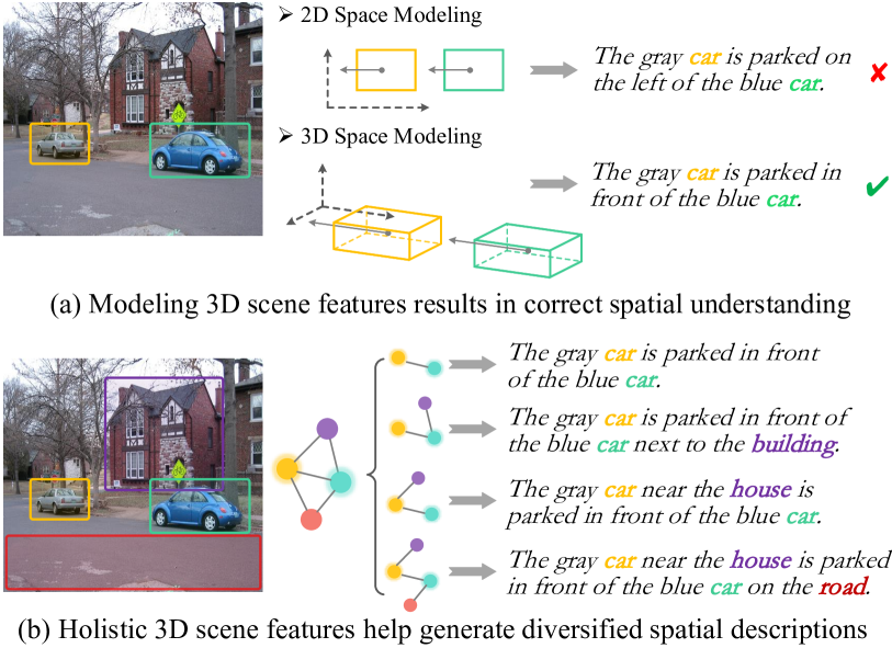
Figure 1: Examples of the visual spatial description.

Zhao et al. (2022) pioneer the VSD task by manually annotating the spatial descriptions to the images based on the visual spatial classification datasets Krishna et al. (2017). Also they solve VSD as a general image-to-text (I2T) task via vision-language pre-trained models (VL-PTMs), i.e., inputting images and outputting texts. However, modeling VSD as a regular I2T job with open-ended VL-PTMs can be problematic. Unlike the existing I2T tasks, such as image captioning Vinyals et al. (2015), verb-specific semantic roles (VSR) guided captioning Chen et al. (2021) and visual question answering (VQA) Antol et al. (2015) that focus on the content semantics understanding, VSD emphasizes more on the spatial semantics reasoning, according to its definition. Thus, directly adapting VSD with general-purpose VL-PTMs will lead to inferior task performances. We note that there are at least two observations that should be taken into account for VSD enhancement.

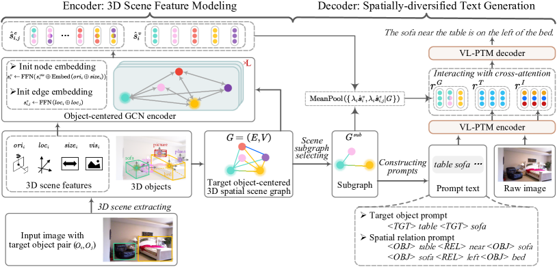
Figure 2: The overview of our proposed framework.

From the image encoding aspect, it is critical to model the holistic 3D scene semantics of the input image. In Zhao et al. (2022), their VL-PTM-based methods model the visual geometrical features at merely 2D flat space (e.g., superficial features). Yet directly perceiving objects from the first-person perspective will inevitably result in skewed angle of view and biased spatial understanding, and thus fail to handle complex cases (e.g. layout overlap, perspective illusion) or generate incorrect descriptions. For example as in Figure 1(a), with the 2D-level visual understanding, the spatial relation between two cars is wrongly decided. As a reference, we human always first project the visual contents into the 3D space and reckon the scene layout and object attributes (e.g., depth, shapes, camera poses), and then narrate the spatial relations based on such holistic 3D clues.

From the text decoding aspect, it is necessary yet challenging to generate diverse sentences of the object pair relation. In generic I2T task, prior methods strengthen the text diversification by equipping with beam search Vijayakumar et al. (2018) or integrating external knowledge Yu et al. (2022). Different from the generic diversified generation, VSD requires the diversification with respect to the spatial descriptions, rather than the diverse linguistics. We can again place the emphasis on the modeling of holistic 3D scene features. For example, with a precise understanding of the spatial relations, it is both viable to generate ‘A is on the left of B’ or ‘B is on the right of A’. Also, as illustrated in Figure 1(b), by comprehensively modeling the surrounding relations of the neighbor objects connecting to the target objects in the holistic scene, more spatially-diverse texts can be yielded via different path traversing.

In this paper, we propose enhancing VSD by modeling the holistic 3D scene semantics. We build an encoder-decoder VSD framework (cf. Figure 2), where the encoder learns the 3D spatial features, and the decoder generates spatially-diversified descriptions based on the spatial semantic features. Specifically, at encoding side, we first employ an off-the-shelf 3D scene extractor Nie et al. (2020) to produce 3D objects and the corresponding scene features (i.e., layout, location, size and visual features) for the input monocular RGB image, via which we build a target object-centered 3D spatial scene graph (namely, Go3D-S²G). We then present an object-centered graph convolutional network (OcGCN) to encode the Go3D-S²G. At decoding side, we devise a scene subgraph selecting (S³) mechanism to sample topologically-diverse object-neighboring subgraphs from Go3D-S²G, which allows to generate descriptions focusing on the near surroundings of target object. Based on the sampled subgraphs, we then create prompt texts to ground the focused objects and their prototype directions. Finally, a backbone VL-PTM is used to encode the prompt texts, input images as well as 3D scene features, then to produce VSD texts.

We experiment on two versions of VSD datasets Zhao et al. (2022), where one is with simple annotations and one has more complex and human-friendly descriptions. The results indicate that our system outperforms the best baseline with significant margins, where our method especially improves on the complex cases, such as layout-overlapped and irregularly-posed objects. We further reveal how the 3D scene graph modeling as well as the S³ mechanism facilitate the task, and also quantify the influence of the external 3D scene extractor. All in all, this work contributes by verifying that modeling the 3D scene of 2D image helps the understanding of visual spatial semantics.

2 Methodology

Problem Definition

Given an image $I$ with two object proposals <$O_{1},O_{2}$> in $I$, VSD generates a sequence of words $S=\{w_{1},...,w_{n}\}$ that describes the spatial relationship between $O_{1}$ and $O_{2}$. The input $O_{1}$ and $O_{2}$ contain the object tags and their 2D location coordinates. Different from image captioning, the generated sentences of VSD must directly or indirectly express the spatial relation between the target objects.

Overall Framework

As shown in Figure 2, our framework (namely 3Dvsd) is built upon an encoder-decoder paradigm, where the encoder is responsible for the 3D scene feature modeling, and the decoder generates spatially-diversified descriptions based on the spatial semantic features learned from encoder.

2.1 Encoder: 3D Scene Feature Modeling

We first extract 3D scene features via an external extractor. Then we build a target object-centered 3D spatial scene graph (Go3D-S²G), which is encoded and propagated with an object-centered GCN (OcGCN).

$vis_{i}$	The flatted ROI feature of object $i$.
$size_{i}$	The length, width, height of object $i$.
$loc_{i}$	The relative centroid coordinates of object $i$.
$ori_{i}$	The rotation value of three degrees of freedom
	of object $i$.

Table 1: Summary of the 3D scene features.

Extracting 3D Scene Features

We adopt the 3D scene extractor as in Nie et al. (2020), which is a joint layout estimator and 3D object detector. It first processes the 2D object detection for the input RGB image, based on which the 3D relative coordinates (location) and pose parameters of all the objects will be estimated. Formally, we set up the world system located at the camera center with its vertical axis perpendicular to the floor, and its forward axis toward the camera, such that the camera pose $R(\beta,\gamma)$ can be decided by the pitch and roll angles $(\beta,\gamma)$. In the world system, an object $O_{i}$ can be determined by a 3D center $loc_{i}\in\mathbb{R}^{3}$, spatial size $size_{i}\in\mathbb{R}^{3}$, orientation angle $ori_{i}\in[-\pi,\pi)^{3}$. Finally, we obtain the $loc_{i}$, $size_{i}$, $ori_{i}$ and the region-of-interest (RoI) $vis_{i}$ (with its representation $r_{i}^{vis}$) of each 3D object, which is summarized in Table 1. We extend the 3D scene generating details at Appendix A.1.

Constructing Target Object-centered 3D Spatial Scene Graph

Based on the 3D objects and the corresponding 3D scene features, we now construct the Go3D-S²G. The graph is centered on the two target objects, placing the focus on the spatial relationships between the target objects and their surrounding neighbor objects in the scene. Technically, we denote Go3D-S²G as $G$ =$(E,V)$, where $V$ is the set of 3D nodes $v_{i}$ (i.e., 3D objects). Note that as the input images are likely to contain some noisy objects that are less-informative to the task, we remove those objects by comparing their confidence $f_{i}$ (i.e., the logit from the object detector) with a threshold $p$. $E$ is the set of edges $e_{i,j}$, consisting three types:

• Target-pair edge, which connects two given target objects.

• Target-surrounding edge, which connects each target object to all their surrounding non-target objects.

• Near-neighbor edge, which connects those non-target objects in near neighbor that may have implicit correlations between each other. We build the edges by calculating their coordinates ($loc_{i}$), with those values larger than a pre-defined threshold $d$ as valid edges.

The edge $e_{i,j}$=1 when there is an edge between $v_{i}$ and $v_{j}$. Figure 3 illustrates the edge constructions.

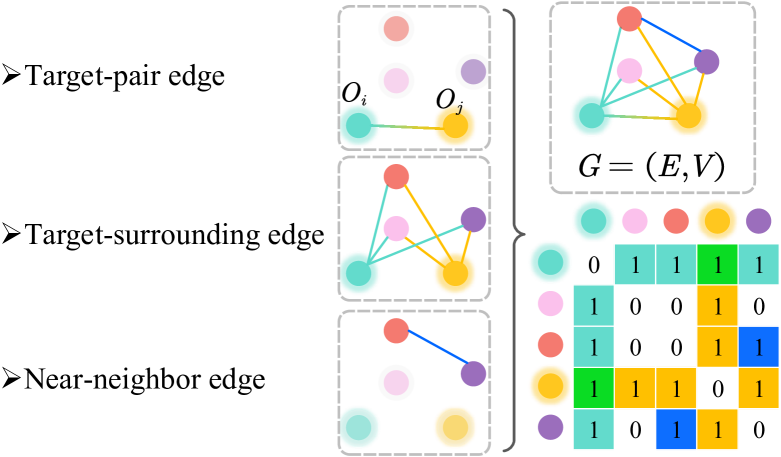
Figure 3: Three types of edges of Go3D-S²G.

Encoding Graph with Object-centered GCN

While graph convolutional network (GCN) Marcheggiani and Titov (2017) has been shown effective for aggregating graph data, it may fail to model the centralization of the target objects of Go3D-S²G structure (as GCN treats all nodes equally). Thus, we devise an object-centered GCN, which advances in modeling both the edge features and the target objects. OcGCN first creates initial representations of node $\bm{s}^{v}_{i}$ and edge $\bm{s}^{e}_{i,j}$.

$$\begin{split}\bm{s}^{pose}_{i}&=\text{Embed}({ori}_{i}\oplus{size}_{i})\,,\\ \bm{s}^{v}_{i}&=\text{FFN}(\bm{s}^{vis}_{i}\oplus\bm{s}^{pose}_{i})\,,\\ \bm{s}^{e}_{i,j}&=\text{FFN}(loc_{i}\oplus loc_{j})\,,\\ \end{split}$$ (1)

where Embed() is the looking-up operation, FFN() is the non-linear feedforward network.

Then, OcGCN updates the Go3D-S²G:

$$\begin{split}\bm{s}^{v}_{i}&=\sigma(\sum_{j=1}\gamma_{i,j}(\bm{W}_{a}\cdot[\bm{s}^{v}_{i^{{}^{\prime}}};\bm{s}^{e}_{i,j};\bm{s}^{v}_{t}]))\,,\\ \gamma_{i,j}&=\frac{e_{i,j}\cdot\exp(\bm{W}_{b}(\bm{s}^{v}_{j^{{}^{\prime}}}\oplus e_{i,j}\oplus\bm{s}^{v}_{t}))}{\sum_{t=1}e_{i,t}\cdot\exp(\bm{W}_{b}(\bm{s}^{v}_{t^{{}^{\prime}}}\oplus e_{i,t}\oplus\bm{s}^{v}_{t}))}\,,\\ \end{split}$$ (2)

where $\bm{s}^{v}_{i^{{}^{\prime}}}$ is the node representation of last layer, as OcGCN has total $L$ layers. $\bm{s}^{v}_{t}$=$\bm{s}^{v}_{O_{1}}\oplus\bm{s}^{v}_{O_{2}}$ is the summary of the two target objects. $[;]$ is the concatenation operation. $\bm{W}_{a},\bm{W}_{b},b$ are learnable parameters. The weight $\gamma_{i,j}^{l}$ reflects the contribution of each object when propagating the spatial attributes towards target objects.

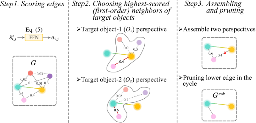
Figure 4: Scene subgraph selecting mechanism.

2.2 Decoder: Spatially-diversified Text Generation

In decoding stage, we use a VL-PLM to generate VSD texts, as shown in Figure 2. We first perform scene subgraph selection over Go3D-S²G, where the diverse local structures lead to spatially-diversified text generation. Also we create prompt texts to hint model to generate relevant contents.

Scene Subgraph Selecting

As cast earlier, we can make use of the neighbor non-target objects of the two target objects in the scene as type of ‘bridges’ to diversify the generation. Thus, we propose a scene subgraph selecting (namely, S³) mechanism to sample sub-structures of Go3D-S²G.

Concretely, S³ contains three steps, as illustrated in Figure 4. First, we calculate the connecting-strength score for each edges in Go3D-S²G via a simple FFN transformation: $a_{i,j}$=FFN($\hat{s}^{e}_{i,j}$), where $\hat{s}^{e}_{i,j}$ is the edge representation of final-layer OcGCN. In the second step, we take a first-order traversal to search the best neighbor nodes of two target objects, respectively, where the best neighbor nodes have the highest connecting scores to their target objects. Note that we only consider the direct neighbor of target objects (i.e., first-order connection), because including nodes in too distant will rather lead to inaccurate descriptions. In the third step, we assemble the two perspective structures into one, and then prune the conflicting edge with lower connecting score if a cycle exists (i.e. two target objects connects to a common neighbor), resulting in a successful subgraph.

It is noteworthy that during training we sample only one subgraph with highest-scored edge, where reparameterization trick Blum et al. (2015) is used for gradient propagation. During inference, we sample multiple scene subgraphs with top-$k$ highest score edges, i.e., giving diverse descriptions.

With the subgraph at hand, we create its representations via a mean-pooling operation over it:

$$\begin{split}\lambda_{i}&=\frac{\delta(v_{i}\in{G}_{sub})+a_{t_{1},i}+a_{t_{2},i}}{\sum_{l\in{G}}\left(a_{t_{1},l}+a_{t_{2},l}\right)}\,,\\ \bm{r}^{G}&=\text{MeanPool}(\{\lambda_{i}\hat{\bm{s}}^{v}_{i},\lambda_{i}\hat{\bm{s}}^{e}_{i,j}|{G}\})\,,\end{split}$$ (3)

where $a_{i,j}$ is the strength score, $t_{1}$ and $t_{2}$ are the target nodes, $\delta(exp)$ funtion outputs 1 when $exp$ is true, otherwise 0 , $\hat{\bm{s}}^{v}_{i},\hat{\bm{s}}^{e}_{i,j}$ are the node and edge representations of last-layer OcGCN. The local scene graph feature $\bm{r}^{G}$ will be used during text generation at following stage.

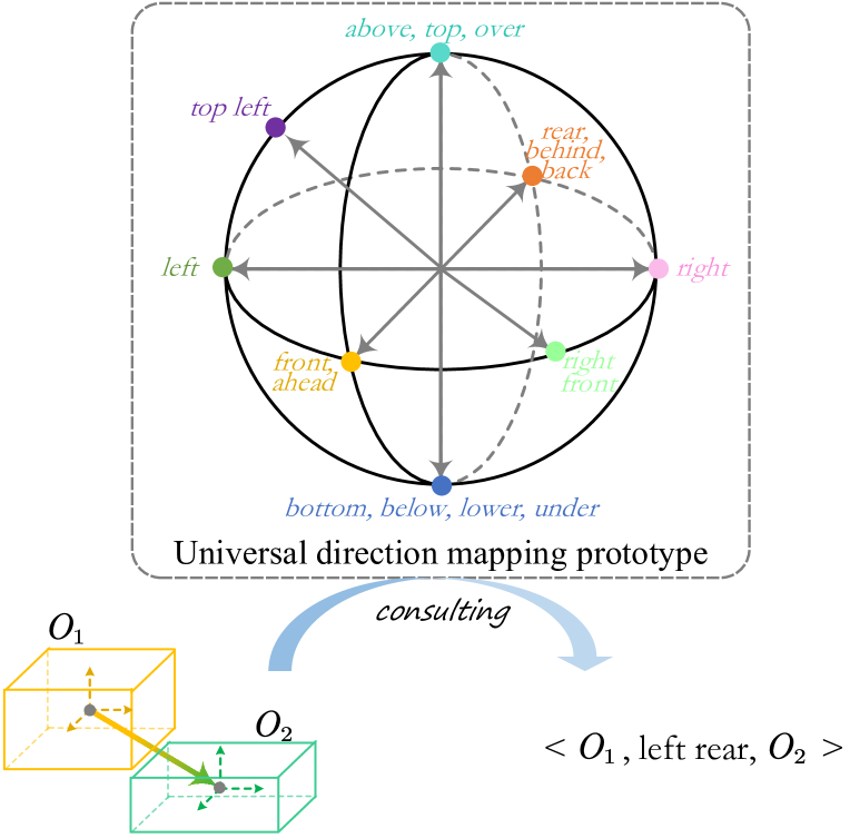
Figure 5: The prototype of direction-term mapping.

Building Directional Prompts

Now we try to guide the VL-PLM to generate contents closely relating to the target objects and the nodes in the sampled subgraph. We thus build two types of prompt texts, 1) target object prompt, e.g.,

<TGT> table <TGT> sofa

and 2) spatial relation prompt, e.g.,

<OBJ> table <REL> near <OBJ> sofa

<OBJ> sofa <REL> left <OBJ> bed

Two types of prompts are concatenated as one via a ‘<SEP>’ token. The former enlightens model what the target objects are, and the latter tells model what possible relational triplets are, i.e., “<object_i, relation, object_j>”, where “relation” is the predefined relation term. For each pair of $O_{i}$, $O_{j}$ in Go3D-S²G, we map their edge $e_{ij}$ to a specific direction term based on their centroid coordinates.

We maintain a prototype of 3D universal direction-term mapping, as shown in Figure 5, where we define 26 directions in the whole sphere, with each direction binding certain directional terms. Even a strong VL-PLM may fail to map a direction to a term accurately. We thus additionally perform pre-training to strengthen the perception of direction.

Pre-definitions
Subject centroid: $x_{s}$, $y_{s}$, $z_{s}$, Object centroid: $x_{o}$, $y_{o}$, $z_{o}$
coordinate system: x-toward, y-up, z-right
$x,y,z\in\left[0,1\right]$
$d_{x}=|x_{s}-x_{o}|\,,d_{y}=|y_{s}-y_{o}|\,,d_{z}=|z_{s}-z_{o}|$
Rule	Direction Term
Front: ($d_{x}>d_{y}$ and $d_{z}$, $d_{x}>0.2$,$x_{s}>x_{o}$)
$d_{y},d_{z}\leq 0.2$	“front”
$d_{y}>0.2,y_{s}>y_{o},d_{z}\leq 0.2$	“front up”
$d_{y}>0.2,y_{s}<y_{o},d_{z}\leq 0.2$	“front down”
$d_{z}>0.2,z_{s}>z_{o},d_{y}\leq 0.2$	“front right”
$d_{z}>0.2,z_{s}<z_{o},d_{y}\leq 0.2$	“front left”
$d_{y},d_{z}>0.2,y_{s}>y_{o},z_{s}>z_{o}$	“front up right”
$d_{y},d_{z}>0.2,y_{s}>y_{o},z_{s}<z_{o}$	“front up left”
$d_{y},d_{z}>0.2,y_{s}<y_{o},z_{s}>z_{o}$	“front down right”
$d_{y},d_{z}>0.2,y_{s}<y_{o},z_{s}<z_{o}$	“front down left”
Back: ($d_{x}>d_{y}$ and $d_{z}$, $d_{x}>0.2$,$x_{s}<x_{o}$)
$d_{x}>0.2,d_{y},d_{z}\leq 0.2$	“back”
Others are similar to front
Up: ($d_{y}>d_{x}$ and $d_{z}$, $d_{y}>0.2$,$y_{s}>y_{o}$)
Others are similar to front
Down: ($d_{y}>d_{x}$ and $d_{z}$, $d_{y}>0.2$,$y_{s}<y_{o}$)
Others are similar to front
Right: ($d_{z}>d_{x}$ and $d_{y}$, $d_{z}>0.2$,$z_{s}>z_{o}$)
Others are similar to front
Left: ($d_{z}>d_{x}$ and $d_{y}$, $d_{z}>0.2$,$z_{s}<z_{o}$)
Others are similar to front
($d_{x},d_{y},d_{z}\leq 0.2$)	“next to”

Table 2: Direction term mapping rules.

The detailed mapping rules of universal 3D direction-term are shown in Table 2. With the predefined 26 directions, we compare the centroid coordinates of a pair of objects to decide the direction terms. Note that according to the rules in Table 2, there may be multiple terms for the same direction, e.g., “left up front” and “up left front” and we keep these redundant terms in our implementation. We add an extra term “next to” to describe the situation that two objects are close to each other. For some types of object that not exists during the 3D Scene Extractor pretraining, we just use their 2D locations and treat the depth coordinate to 0.

Moreover, we conduct a pre-training to strengthen the perception of direction for VL-PTM. Concretely, we utilize the 3D scene extractor and relation triplets ground-truth in VSD dataset to generate a set of pseudo data. For example, if we have two target objects $O_{1}$, $O_{2}$ with theirs names $Tag_{1}$, $Tag_{2}$ ,ground-truth relation term $Rel_{g}$ (in VSD annotations), and 2D boxes $Box_{1}$, $Box_{2}$, we could get their 3D centroid coordinates $loc_{1}$, $loc_{2}$ through off-the-shelf 3D scene extractor. Then we map the 3D centroid coordinates to 3D direction term $Rel_{p}$. We use “<OBJ> $Tag_{1}$ <REL> $Rel_{p}$ <OBJ> $Tag_{2}$” as inputs and “$Tag_{1}$, $Rel_{g}$, $Tag_{2}$” as outputs to train the VL-PTM. Moreover, we randomly replace the $Rel_{g}$ with some synonyms for data augmentation.

Generating Text

Finally, we feed the prompt text and the raw image as input into our backbone VL-PLM encoder, where the resulting representations $\bm{r}^{T}$ and $\bm{r}^{I}$ and the local scene graph feature $\bm{r}^{G}$ are fused together via cross-attention, i.e., $\bm{r}$=CrossAtt($\bm{r}^{G},\bm{r}^{T},\bm{r}^{I}$). The VL-PLM decoder then performs text generation based on $\bm{r}$.

		VSD-v1					VSD-v2
		BLEU-4	METEOR	ROUGE	CIDEr	SPICE	BLEU-4	METEOR	ROUGE	CIDEr	SPICE
$\bullet$ VL-PTMs
	Oscar	37.17	35.06	66.47	427.21	67.41	20.90	23.83	50.96	221.61	44.12
	VL-Bart	52.71	41.96	77.57	471.21	67.83	23.78	24.83	48.49	253.26	45.04
	VL-T5	52.58	41.94	77.63	472.24	67.90	23.83	24.26	53.51	255.51	46.86
	OFA	53.59	41.74	77.68	469.23	67.03	24.53	24.93	54.27	257.29	45.63
$\bullet$ VL-PTMs + VSRC Zhao et al. (2022)
	VLBart-ppl	53.49	42.14	77.79	474.34	67.97	24.44	24.08	53.80	256.52	45.16
	VLT5-ppl	53.71	42.56	78.33	480.32	68.72	23.79	24.49	54.49	256.70	46.04
	VLBart-e2e	53.60	42.45	78.15	476.47	68.18	24.71	24.41	54.22	258.18	45.79
	VLT5-e2e	54.31	42.63	78.38	481.13	68.74	24.47	24.50	54.52	261.70	46.07
$\bullet$ VL-PTMs + 3D scene features
	3Dvsd (Ours)	54.85	43.25	79.38	483.05	68.76	26.40	26.87	55.76	272.93	46.97
		(+0.54)	(+0.62)	(+1.00)	(+1.92)	(+0.02)	(+1.87)	(+1.94)	(+1.24)	(+11.23)	(+0.11)

Table 3: Main results on two datasets. Bold numbers are the best, and underlined ones are the second best.

3 Experiments

3.1 Settings

Dataset

We evaluate our model on two datasets: VSD-v1 and VSD-v2 Zhao et al. (2022). VSD-v1 is the initial version of VSD datasets, which has a large scale but simple annotations. VSD-v2 has the same image source while more complex and human-friendly descriptions, which is more challenging. We use the original split of train/dev/test set of each dataset.

Implementation

Our model takes the pre-trained 3D extractor from Nie et al. (2020), containing the layout estimation network and the 3D object detection network. The hidden size of OcGCN is 768 which is the same with text decoder. The dimension of edge feature $\bm{s}^{e}_{i,j}$ is also 768. We adopt the OFA_base as our backbone VL-PLM.

Evaluation

We make comparisons with 1) the existing popular image-to-text VL-PLMs, including OSCAR Li et al. (2020), VLT5/VLBart Cho et al. (2021), OFA Wang et al. (2022b); 2) the models introduced in Zhao et al. (2022), including the pipeline (ppl) and the end-to-end (e2e) paradigms. Zhao et al. (2022) use the visual spatial relations classification (VSRC) results as intermediate features for VSD. Following Zhao et al. (2022), we adopt five automatic metrics to evaluate performances, including BLEU-4, MENTEOR, ROUGE, CIDEr and SPICE. We measure the diversity with three metrics, i.e., mBLEU-4, BLEU-4@K and SPICE@K. All the used VL-PLMs are the base version. Our results are the average scores over five runs. Appendix $\S$B.3 details all the experimental settings.

B4	M	R	C	S
VL-T5	29.41	28.67	59.23	294.81	50.04
OFA	33.14	30.02	60.87	290.93	49.23
VLT5-e2e	29.64	28.88	60.13	291.32	51.01
3Dvsd	39.29	34.27	67.88	328.56	55.42

Table 4: Results on hard cases in VSD-v2, where the images come with layout-overlapped and irregularly-posed target objects.

3.2 Main Observations

		BLEU-4	SPICE
	3Dvsd (Full)	26.40	46.97
1-4	w/o Go3D-S2G	23.31(-3.09)	43.89(-3.08)
	w/o OcGCN	24.51(-1.89)	46.85(-0.12)
	w/o S3 mechanism	25.19(-1.21)	46.38(-0.59)
	w/o Dir-term Prompts	26.18(-0.22)	46.17(-0.80)

Table 5: Ablation results (VSD-v2). ‘w/o Go3D-S²G’ means ablating the graph modeling of 3D scene feature, while instead using the embedded vectors $\bm{s}_{i}^{v}$ for text generation. ‘w/o OcGCN’ means replacing OcGCN encoder with the vanilla GCN. ‘ w/o S³’ means replacing with beam search decoding. ‘Dir-term Prompts’ represents the directional term prompts.

Main Results

As shown in Table 3, overall, the VSD-v2 can be more challenging than VSD-v1, where model scores on all the metrics are lower. Also we see that four different VL-PTMs show the similar level of performances, due to their general purpose of pre-training for multimodal learning. By taking advantages of the VSRC features, Zhao et al. (2022)’s methods outperform the baseline vanilla VL-PTMs on the task. However, the improvements from Zhao et al. (2022)’s models can be incremental, due to the reason that Zhao et al. (2022) model the input images with only 2D information. On the contrast, our proposed 3Dvsd model achieves significant improvement over the baselines cross two datasets on all the metrics, evidently demonstrating its efficacy.

In addition, our model shows larger improvements on the harder VSD-v2 data than that on VSD-v1. To directly measure the capability of our method, we further collect a subset from VSD-v2, where the target objects in images are irregularly-posed with complex spatial relation, and also there are overlapped layouts. We perform experiments on the set, where the results are shown in Table 4. We can find that our 3Dvsd model improves the best-performing baseline with marked boosts, i.e., 1.87 BLEU-4, 1.94 METROR, 1.24 ROUGE and 5.11 CIDEr. This significantly indicates that our method is capable of well understanding the visual spatial semantics and thus generating more diverse and flexible VSD sentences.

Model Ablation

Now we quantify the contribution of each design in our systems via model ablation, as shown in Table 5. First, we can see that the 3D scene feature from Go3D-S²G graph modeling gives the biggest influences, i.e., contributing 3.09 BLEU-4 and 3.08 SPICE scores. Besides, the OcGCN encoder, the S³ mechanism as well as the direction-term prompting also plays an essential role to the overall system, respectively.

Evaluation on Spatial-diversity Generation

As we equip our system with the S³ mechanism, we can generate spatially-diversified texts. Next, we directly assess the ability on the generation spatial-diversification. We first make comparisons with the beam search method using automatic metrics Deshpande et al. (2019), including mBLEU-4, BLEU-4@K and SPICE@K. mBLEU-4 compares the 4-gram matching between one of the generated sentence and the remaining generated sentences for an image, and thus lower mBLEU-4 score means more diversity. BLEU-4@K and SPICE@K represent the highest BLEU-4 and SPICE score for the top-$k$ generated sentences for an image, where higher BLEU-4@K and SPICE@K prove that the a model can keep better semantics accuracy while generating diverse results. As shown in Table 6, our S³ mechanism achieves lower mBLEU-4 and higher BLEU-4@K and SPICE@K, demonstrating that our method could generate diversified descriptions with enough semantics accuracy.

		K=5 Samlpling
		mBLEU-4$\downarrow$	BLEU-4@K$\uparrow$	SPICE@K$\uparrow$
Beam Search
	VL-T5	8.62	33.02	60.55
	OFA	7.77	32.72	60.37
	3Dvsd	7.6	33.12	60.67
Scene Subgraph Sampling
	3Dvsd	5.01	34.44	61.99

Table 6: Auto-evaluation on spatial diversification.

		Spatial Acc.$\uparrow$	Spatial Div.$\uparrow$	Fluency$\uparrow$
Beam Search
	VL-T5	3.05	2.91	4.33
	OFA	3.14	2.94	4.39
	3Dvsd	3.13	3.10	4.49
Scene Subgraph Sampling
	3Dvsd	3.19	3.98	4.53

Table 7: Human evaluation (with Likert 5-scale) on generation diversification. We randomly select 100 samples from VSD-v2.

Figure 6: Comparison of 2D and 3D method on VSDv2.

We also provide a human evaluation to describe spatial diversity with respect to the Spatial Accuracy, Spatial Diversity and Fluency. We ask 10 English speakers to answer the 5-point Likert scale on 100 samples, where the average results are shown in Table 7. Overall, all the models can achieve competitive score on language fluency, thanks to the superiority of VL pretraining. Also the tendencies of spatial accuracy and diversity is consistent with the automatic evaluation. Remarkably, our S³ mechanism shows the best capability on spatial diversity, demonstrating its effectiveness.

Figure 7: Ablation results of 3D features on VSDv2.

3.3 Analyses and Discussions

To gain an in-depth understanding of our method’s strengths, we try to answer following research questions via further analyses:

$\bullet$ RQ1: How 3D scene features help understanding the spatial semantics of input images?

A: The key of our method is the leverage of 3D scene features. Now, we first consider downgrading the 3D features into the 2D ones, such that we can gain the perception of its necessity. To ensure the fair comparison, we remove the 3D scene extractor and replace the 3D pose feature $pose_{i}$ (Eq. 1) with the 2D size. Also we replace the 3D coordinates by 2D coordinates. And the other settings are kept the same. As shown the results in Figure 6, the 2D scene modeling results in the markedly performance decrease.

We can further quantify the contributions of each type of 3D features via feature ablation, including the orientation feature $ori_{i}$ and the size feature $size_{i}$. As seen in Figure 7, both 3D orientation and 3D size features contribute to the overall system. Also the influence on SPICE is larger, which indicates that the orientation and size of the objects especially help recognize the spatial relation. Finally, in Figure 8 we empirically show the OcGCN’s kernel weight $\gamma_{i,j}$ (Eq. 2) on two pieces of instances, where the attention values reflect the contribution of each object. It is clear that our model has successfully captured the spatial semantics of the target object pairs.

$\bullet$ RQ2: How does S³ mechanism aid the diversified spatial description generation?

Figure 8: Qualitative results of generated descriptions with beam search decoding and S³ mechanism, respectively.

Figure 9: Performances on the indoor (NYU) and outdoor (Visual Genome and Flickr) input images. The pie chart shows the data proportion.

A: Next, we consider investigating how exactly the S³ mechanism contribute to the spatial description generation. Through our S³ mechanism, we could generate 4 types of subgraphs: 1) with only target nodes (2-hop); 2) with one non-target neighbor node linked with subject node (3-hop-s); 3) with one non-target neighbor node linked with object node (3-hop-o); 4) with two non-target neighbor nodes. In our implementation, we use a threshold $p_{cut}$ to filter out edges with very low scores. Figure 10 show the distribution of four subgraphs with $p_{cut}$=0.1 or 0.2. We see that different $p_{cut}$ values help generates spatial descriptions with varying numbers of objects attended into the subgraphs. That is, S³ mechanism aids the diversified spatial description generation by producing multiple heterogeneous subgraphs structures.

(a) $p_{cut}=0.2$

(b) $p_{cut}=0.1$

Figure 10: Distribution of subgraph types.

We also empirically show the qualitative results in Figure 8. We notice that the beam search method can generate multiple alternative texts in both cases, where unfortunately the diversification on describing the spatial relation is much inferior and limited. In contrast, with our S³ method, the system generates spatial-diversified descriptions for both two images. Some surrounding objects, e.g., ‘shelf’, ‘table’, ‘door’ in the first case and ‘chair’, ‘bed’, ‘shelf’ and ‘desk’ in the second case, are leveraged to aid describe the target objects.

$\bullet$ RQ3: To what extent the external 3D scene extractor quality influence the VSD performances?

A: As we obtain the initial 3D scene features from the external extractor, the quality of the extractor is key to our final VSD performance. Note that the off-the-shelf 3D extractor is trained on a datasets of indoor scenes, while in VSD dataset the images contain both types of indoor (NYU) and outdoor (Visual Genome (VG) and Flickr). As shown in Figure 9, the indoor images actually are the minority in our VSD data. Here we perform analysis to valid the influence on 3D scene extractor. We split the VSD-v2 test set into indoor and outdoor subsets according to the domain types. Then we run our model on the two sets separately. As shown in the figure, the results on the indoor NYU set exceed those on the outdoor VG&Flickr set clearly, demonstrating the domain shift issue in our system. Given that our system has already secured considerable performance increase than existing models, we presume that when obtaining a 3D extractor capable of detecting higher-quality 3D scene features for any domain and scenario, our method has the greater potential to gain more task improvements.

4 Related Work

Image-to-text (I2T) is a fundamental task category of the vision-language multimodal topic. Existing I2T tasks, e.g., image captioning Vinyals et al. (2015); Cornia et al. (2019); Mathews et al. (2018) and VQA Antol et al. (2015); Lubna et al. (2019); Manmadhan and Kovoor (2020), attempt to generate textual pieces to understand the image content semantics through different perspectives. VSD is also a subtask of I2T, which however places the focus on the spatial semantics understanding. Within recent years, VL-PTMs are extensively employed for the I2T tasks, which have helped achieve state-of-the-art performances on many benchmarks Lu et al. (2019); Chen et al. (2019); Zhou et al. (2020); Li et al. (2020); Wang et al. (2022b). Prior VSD study Zhao et al. (2022) has benchmarked the VSD task with these general-purpose VL-PTMs. Unfortunately, different from the content-semantic I2T tasks, the goal of VSD is to grasp the spatial semantics.

This work also relates to the theme of visual spatial understanding, which has been intensively investigated in the past years. Yang et al. (2019); Jänner et al. (2018) propose the visual spatial relation classification (VSRC) task, aiming to predict whether a spatial description is reasonable for the input image. Differently, VSD aims to directly generate the descriptions of the spatial relations. The bottleneck of visual spatial understanding tasks is the capturing of spatial semantics. Thus, in this paper, we propose improving the visual spatial understanding for VSD via modeling the holistic 3D scene features. Our work takes the advancements from the topic of 3D scene parsing Huang et al. (2018a, b); Nie et al. (2020); Zhang et al. (2021), which reconstructs the 3D scene from a single RGB image. By using the 3D scene features, e.g., 3D layout and 3D object, we achieve the goal of more in-depth understanding of the spatial semantics.

5 Conclusion

In this work we incorporate the 3D scene features for improving the visual spatial description (VSD) task. We first employ an off-the-shelf 3D scene extractor to produce 3D objects and scene features for the input images. We then build a target object-centered 3D spatial scene graph (Go3D-S²G) structure, which is encoded with an object-centered graph convolutional network. Next, we devise a scene subgraph selecting mechanism to sample topologically-diverse subgraphs from Go3D-S²G, where the local features are used to guide to generate spatially-diversified descriptions. On the VSD datasets our framework shows superiority on the task, especially for solving the complex cases, such as layout-overlapped and irregularly-posed object. Meanwhile our method can produce more spatially-diversified generation. Finally, we demonstrate the influence of quality of the external 3D scene extractor.

Limitations

This work has one major risk. As the main idea proposed in this work heavily relies on the external 3D scene extractor, the quality of extractor on our used VSD images largely influences the task performance. However, we reveal in analysis that although suffering from the domain shift issue by the out-of-domain 3D scene extractor, our method still improves the VSD task. We show that when handling the in-domain VSD images as used for training the 3D scene extractor, the VSD performance has been boosted remarkedly. Thus, with better a 3D scene extractor, it can be expected that our system will exhibit much stronger capability and advance the VSD task more significantly.

Appendix A Model Specification

Here we provide the detailed calculations of our system. For the MeanPool operation in Equation 3, we calculate $\textbf{r}^{G}$ as:

$$\begin{split}\textbf{r}^{G}=\frac{1}{M^{2}}\sum_{i\in G}\sum_{j\in G}\lambda_{i}\left(\hat{\bm{s}}^{v}_{i}\oplus\hat{\bm{s}}^{e}_{i,j}\right)\end{split}$$ (4)

where $M$ is the node number of the Go3D-S²G, $\lambda_{i}$ is a weight expansion (shown in Equation 3), which could capture the subgraph features with a very high weight, $\hat{\bm{s}}^{v}_{i}$ and $\hat{\bm{s}}^{e}_{i,j}$ are the node and edge representations of last-layer OcGCN.

For VL-PTM encoding, we adopt the approach in OFA model Wang et al. (2022b). The input image $I$ is first embedded by a inbuilt ResNet and flatted to a tokenized visual feature. Then the visual features are projected to the encoder model dimension, obtaining the global visual feature $\bm{r}^{I}$. The process could be formalized as:

$$\begin{split}\hat{\bm{r}}^{I}&=\text{ResNet}(I),\\ \bm{r}^{I}&=W_{v}\hat{\bm{r}}^{I}+b_{v},\end{split}$$ (5)

where $W_{c}$ and $b_{c}$ are model parameters. Then the tokenized visual features are concatenated with embedded text sequence as the inputs of VL-PTM encoder:

$$\begin{split}\bm{h}^{I,T}&=\text{Encoder}(\bm{r}^{I}\oplus\bm{r}^{T}).\end{split}$$ (6)

After that, the encoder outputs and graph feature $\bm{r}^{G}$ are fused through cross-attention in VL-PTM decoder. The cross-attention operation in a transformer unit could be formalized as:

$$\begin{split}\bm{X}&=\left\{\bm{r}^{G};\bm{h}^{I,T}\right\},\\ \bm{K}=\bm{W}_{k}\bm{X},\bm{V}&=\bm{W}_{v}\bm{X},\bm{Q}=\bm{W}_{q}\bm{D_{h}},\\ \textit{Attention}(\bm{Q},\bm{K},\bm{V})&=\textit{softmax}\left(\frac{\bm{Q}\bm{K}}{\sqrt{d}}\right)\bm{V},\end{split}$$ (7)

where $\bm{r}_{G}$ is the graph feature, $\bm{h}^{I,T}$ is the encoder outputs, $\bm{W}_{k},\bm{W}_{v},\bm{W}_{q}$ are model parameters, $d$ is the out dimension of $\bm{W}_{v}$, $\bm{D}_{h}$ is the outputs of self-attention unit in Transformer decoder.

A.1 3D Scene Extracting

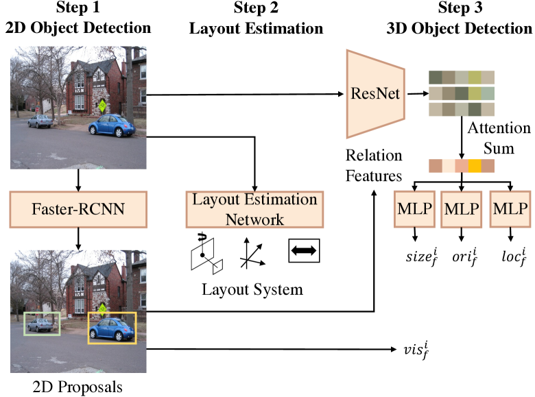
Figure 11: The framework of 3D scene extractor.

We employ an external 3D scene extractor from Nie et al. (2020), which is pretrained on the SUN RGB-D dataset Song et al. (2015). The model contains three modules: 1. Layout Estimation Network (LEN); 2. 3D Object Detection Network (ODN); 3. Mesh Generation Network (MGN). In our framework, we only use LEN and ODN, which outputs the layout coordinates system and the 3D location and pose of each object. We also need a 2D Object Detector to generate appearance feature and 2D box as the inputs for ODN. We directly borrow the Faster-RCNN Ren et al. (2015) to process the images to obtain the necessary RoI features, boxes, and object tags. For the LEN, we need the camera intrinsic parameters to adjust the coordinates system. However, the VSD dataset does not provide this information of the images. We just generate a pseudo camera intrinsic matrix for all the images in our implementation. The method works in VSD because we do not need the accurate location of each object, we just need to capture the relative relations among the object pairs. Thus, the distortion of absolute coordinates will hardly impact the final results of VSD. As shown in Figure 12, though the 3D boxes are distorted, their relative spatial relations remain unchanged.

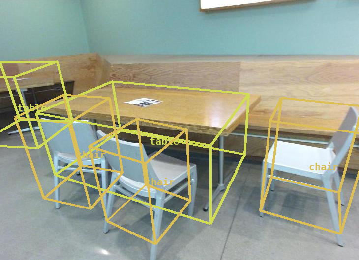
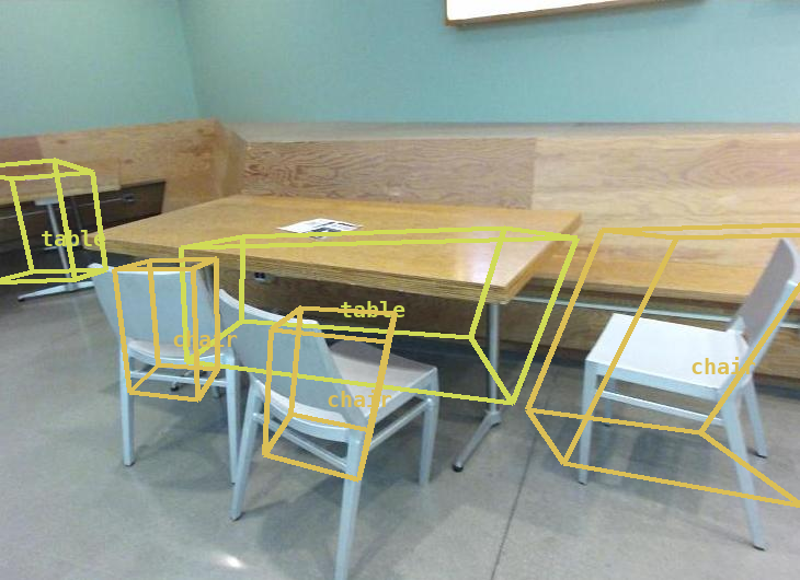
Figure 12: Comparsion of 3D boxes between different camera intrinsics.

A.2 Spatial Scene Graph Creating

Input: max object number $N$,

   two target objects index $o_{1},o_{2}$,

   confidency of each object $f$,

   centroid of each object $C$,

   distance threshold $d$,

   noise confidency threshold $p$

Output: adjacency matrix $\bm{A}^{N\times N}$

initialization: $\bm{A}$ = 0.

// target object edges

$\bm{A}$[$o_{1}$,:] = 1, $\bm{A}$[:, $o_{1}$] = 1,

$\bm{A}$[$o_{2}$,:] = 1, $\bm{A}$[:, $o_{2}$] = 1,

// add special edges

for i in $N$ do

       for j in $N$ do

             dist = $||C_{i}-C_{j}||$

             if dist > $d$ then

                   $\bm{A}_{ij}$ = 1

             end if

            

       end for

      

end for

// remove noise objects

for i in $N$ do

       if $f_{i}<p$ and $o_{i}$ is not target object then

             $\bm{A}$[i,:] = 0, $\bm{A}$[:,i] = 0

       end if

      

end for

Algorithm 1 Go3D-S²G Creating

The detailed algorithm of S³ is shown in Algorithm 1. Suppose that the max object number is $N$ ($N$=36 in our implementation). We first initialize an $N\times N$ adjacency matrix $\bm{A}=\bm{0}$. When adding the Target-pair and Target-surrounding edges, we set the columns and rows of the target object index to 1. When adding the Near-neighbor edge, we traverse the edges and set the one with $dist$ > $d$ in $\bm{A}$ to 1. At last, we should remove the edges of noisy objects, setting the related items of A to 0.

A.3 Overall Training Procedure

We have several pretrained external modules in our system. First, we prepare the pretrained ResNet for image embedding, which will be used in 3D layout estimation, 3D object detection and the OFA image embedding. Before training, we use the pretrained Faster-RCNN to preprocess all the images for 2D object detection, obtaining the 2D boxes and RoI features. We also prepare the 3D scene extractor pretrained on SUNRGB-D with the method in Nie et al. (2020).

Then we collect the three modules and train our whole system, where the 3D extractor and the decoder (VL-PTM) are initialized by pretrained parameters. The OcGCN and other parameters (e.g. edge embedding, connecting-strength scorer) are initialized randomly. Before global training, we pretrain the VL-PTM with direction terms as Table 2. During global training, the 3D scene extractor are frozen while others will be updated.

We have two main training targets, e.g., the cross-entropy between Vl-PTM decoder outputs and the ground-truth description of VSD $\mathcal{L}_{t}$, and the cross-entropy between connecting-strength score distribution and target object index $\mathcal{L}_{c}$:

$$\begin{split}\mathcal{L}_{t}&=-\sum_{l=1}^{N_{w}}\log p_{\theta}\left(y_{l}|\bm{x},\bm{y}_{<l}\right),\\ \mathcal{L}_{c}&=-\sum_{i=1}^{N}\delta(i\in O_{g})(\log a_{t_{1},i}+loga_{t_{2},i}),\end{split}$$ (8)

where $N_{w}$ is the text length, $\bm{x}$ is the VL-PTM encoder outputs and $y_{l}$ is decoder outputs in the $l$-th step , $N$ is the node number of Go3D-S²G, $a_{i,j}$ is connecting-strength score during S³, $t_{1},t_{2}$ are the two target objects, $O_{g}$ is a set that contains the objects appear in the ground-truth description, and $\delta\left(\cdot\right)$ is the two value function that outputs 1 when $\cdot$ is true, otherwise 0. We obtain $O_{g}$ by string searching in the descriptions. Then the final loss is $\mathcal{L}=\mathcal{L}_{t}+\mathcal{L}_{c}$.

Appendix B Experiment Specification

B.1 Data Analyses

Figure 13: Top 20 objects distribution in VSD dataset.

Object Types

wall, floor, cabinet, bed, chair,

sofa, table, door, window, bookshelf,

picture, counter, blinds, desk, shelves,

curtain, dresser, pillow, mirror, floor,

clothes, ceiling, books, refridgerator, television,

paper, towel, shower curtain, box, whiteboard,

person, night stand, toilet, sink, lamp,

bathtub, bag, other

Table 8: Objects in SUNRGB-D dataset.

The VSD dataset contains images from Visual Genome, Flickr, and NYU-Depth Zhao et al. (2022); Yang et al. (2019), where NYU-Depth is the indoor dataset Silberman et al. (2012).

Figure 13 shows the distribution of object tags in the VSD dataset. Table 8 lists the object types in SUNRGB-D dataset which are used to pretrain 3D scene extractor. There are several common types, such as “person”, “table”, “chair”, “wall” and “window”. Thus the 3D scene extractor could achieve a comparable performance in VSD. For other object types, the built-in 2D object detector (pretrained on VG or COCO) could provide a passable 2D location information.

There are two versions of VSD dataset released, where the VSD-v1 contains large-scale while relative simple descriptions and the VSD-v2 contains small-scale while diversified descriptions. The two versions share the same image set. The statistics of the two datasets are shown in Table 9. Figure 14 shows the difference between the annotations of the two datasets. The annotated sentence in VSD-v1 is relative short and simple while those in VSD-v2 contains more semantics and be more challenging.

B.2 Extended Experimental Implementations

Data Preprocess

For memory space and time saving, we preprocess the data through Faster-RCNN to obtain the RoI featues, object tags and 2D boexs and save them to files. For 3D scene extractor, we also preprocess the images, saving their ResNet features to files.

	#Img	VSD-v1		VSD-v2
		#SENT	AvgLEN	#SENT	AvgLEN
Train	20,490	116,791	7.35	22101	8.88
Dev	2,927	16,823	7.33	3140	8.85
Test	5,855	10,038	8.04	5.34	9.00

Table 9: The statistics of the two versions of VSD dataset.

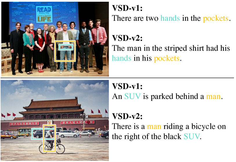
Figure 14: Comparison between annotations of VSD-v1 and VSD-v2.

VL-PTM Configuration

For fairly comparison, we employ the OFA-base as our VL-PTM, which has the similar scale of parameters to the baselines. The layers number is 6 for both encoder and decoder, and the head number of the multi-head attention is 6 as well. Besides OFA, we can use any type of VL-PTMs such as VLT5/VLBart, or combination of single VL encoder and text decoder, such as “CLIP-GPT”, “ViT-GPT”. For more comparison, we leave them in future works.

		K=5 Samlpling			K=10 Samlpling
		mBLEU-4$\downarrow$	BLEU-4@K$\uparrow$	SPICE@K$\uparrow$	mBLEU-4$\downarrow$	BLEU-4@K$\uparrow$	SPICE@K$\uparrow$
Beam Search
	VL-T5	8.62	33.02	60.55	8.02	33.27	61.11
	OFA	7.77	32.72	60.37	7.41	33.09	61.06
	Ours	7.6	33.12	60.67	7.38	33.46	61.31
Scene Subgraph Sampling
	Ours	5.01	34.44	61.99	4.83	34.75	62.61

Table 10: Diversity evaluation results in VSD-v2.

B.3 Hyperparameters

Hyper-param.	Value
dimension of ROI feature	2048
dimension of OFA hiddens	768
dimention of edge feature	64
layer number of GCN	3
max object number	36
distance threshold $d$	0.2
confidency threshold $p$	0.7
S$3$ cutting threshold $p_{cut}$	0.1
max text length	40
optimizer	AdamW
warm up ratio	0.05
weight decay	0.01
Adam $\epsilon$	1e-6
Adam $\beta_{1}$	0.9
Adam $\beta_{2}$	0.999
dropout	0.1
learning rate	5e-5
bach size	16
epoch	30
beam search number	5

Table 11: Model hyperparameters.

Table 11 lists the hyperparameters of our implementation.

B.4 Baselines

We use some strong image-to-text models as our baselines.

• Oscar Li et al. (2020) is a BERT-like visual-language pretrained model, only containing the Transformer encoder. Oscar takes tokenized RoI features of the image as visual inputs. This model has shown strong performance on Image Captioning and VQA.

• VLT5/VLBart Cho et al. (2021) are continue pretrained on image-to-text tasks from generative encoder-decoder language model Bart and T5. Previous work Zhao et al. (2022) has proven their capability on solving VSD task.

• OFA Wang et al. (2022b) is a new vision-language model, which are pretrained by a mount of vision-language multi-modal tasks. It has achieved several SoTA results on existing image-to-text tasks.

Appendix C Extended Experiments

C.1 Diversity Evaluation

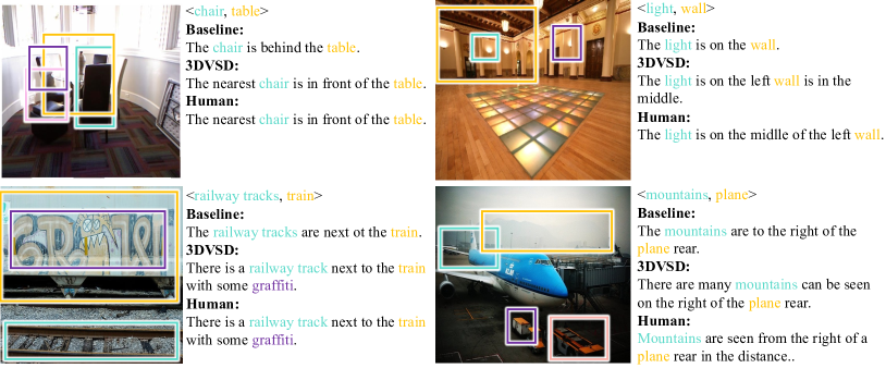
Figure 15: Cases comparison among models and human.

We compare more results of sampling scale for diversity evaluations. Figure 10 reports the results of K=5 and K=10 on VSD-v2. The tendency of K=10 is consistent with that of K=5, where the S³ achieves lower mBLEU-4 and higher BLEU-4@K and SPICE@K.

For human evaluation, our 5-point Likert scale is designed as follows:

• Spatial Accuracy: The sentences correctly describe the spatial relationship of the target objects.

• Spatial Diversity: These sentences describe diversified spatial semantics.

• Fluency: The sentences are readable and not different from human sentence-making.

Each question will be answered by a number from 1 to 5, denoting “Strongly Disagree”, “Disagree”, “Neither disagree nor agraa”, “Agree” and “Strongly agree”. We select 100 samples and generated 5 sentences for each, and sent them to the evaluators for scoring.

C.2 More Case Study

Figure 15 provides some more qualitative comparisons among models and human. Compared with baselines, our model could generate description more like human-made.

References

- Antol et al. (2015) Stanislaw Antol, Aishwarya Agrawal, Jiasen Lu, Margaret Mitchell, Dhruv Batra, C. Lawrence Zitnick, and Devi Parikh. 2015. VQA: visual question answering. In Proceedings of the ICCV, pages 2425–2433.
- Blum et al. (2015) Avrim Blum, Nika Haghtalab, and Ariel D. Procaccia. 2015. Variational dropout and the local reparameterization trick. In Proceedings of the NIPS, pages 2575–2583.
- Castaman et al. (2021) Nicola Castaman, Elisa Tosello, Morris Antonello, Nicola Bagarello, Silvia Gandin, Marco Carraro, Matteo Munaro, Roberto Bortoletto, Stefano Ghidoni, Emanuele Menegatti, and Enrico Pagello. 2021. RUR53: an unmanned ground vehicle for navigation, recognition, and manipulation. Advanced Robotics, 35(1):1–18.
- Chen et al. (2021) Long Chen, Zhihong Jiang, Jun Xiao, and Wei Liu. 2021. Human-like controllable image captioning with verb-specific semantic roles. In Proceedings of the CVPR, pages 16846–16856.
- Chen et al. (2019) Yen-Chun Chen, Linjie Li, Licheng Yu, Ahmed El Kholy, Faisal Ahmed, Zhe Gan, Yu Cheng, and Jingjing Liu. 2019. UNITER: learning universal image-text representations. CoRR, abs/1909.11740.
- Cho et al. (2021) Jaemin Cho, Jie Lei, Hao Tan, and Mohit Bansal. 2021. Unifying vision-and-language tasks via text generation. In Proceedings of the ICML, pages 1931–1942.
- Cornia et al. (2019) Marcella Cornia, Lorenzo Baraldi, and Rita Cucchiara. 2019. Show, control and tell: A framework for generating controllable and grounded captions. In Proceedings of the CVPR, pages 8307–8316.
- Deshpande et al. (2019) Aditya Deshpande, Jyoti Aneja, Liwei Wang, Alexander G. Schwing, and David A. Forsyth. 2019. Fast, diverse and accurate image captioning guided by part-of-speech. In IEEE Conference on Computer Vision and Pattern Recognition, CVPR 2019, Long Beach, CA, USA, June 16-20, 2019, pages 10695–10704. Computer Vision Foundation / IEEE.
- Heuser et al. (2020) Svenja Heuser, Béatrice Arend, and Patrick Sunnen. 2020. Reading aloud in human-computer interaction: How spatial distribution of digital text units at an interactive tabletop contributes to the participants’ shared understanding. In Proceedings of the HCI, pages 117–134.
- Huang et al. (2018a) Siyuan Huang, Siyuan Qi, Yinxue Xiao, Yixin Zhu, Ying Nian Wu, and Song-Chun Zhu. 2018a. Cooperative holistic scene understanding: Unifying 3d object, layout, and camera pose estimation. In Proceedings of the NeruIPS, pages 206–217.
- Huang et al. (2018b) Siyuan Huang, Siyuan Qi, Yixin Zhu, Yinxue Xiao, Yuanlu Xu, and Song-Chun Zhu. 2018b. Holistic 3d scene parsing and reconstruction from a single RGB image. In Proceedings of the ECCV, pages 194–211.
- Jänner et al. (2018) Michaela Jänner, Karthik Narasimhan, and Regina Barzilay. 2018. Representation learning for grounded spatial reasoning. Trans. Assoc. Comput. Linguistics, 6:49–61.
- Krishna et al. (2017) Ranjay Krishna, Yuke Zhu, Oliver Groth, Justin Johnson, Kenji Hata, Joshua Kravitz, Stephanie Chen, Yannis Kalantidis, Li-Jia Li, David A. Shamma, Michael S. Bernstein, and Li Fei-Fei. 2017. Visual genome: Connecting language and vision using crowdsourced dense image annotations. International Journal of Computer Vision, 123(1):32–73.
- Li et al. (2020) Xiujun Li, Xi Yin, Chunyuan Li, Pengchuan Zhang, Xiaowei Hu, Lei Zhang, Lijuan Wang, Houdong Hu, Li Dong, Furu Wei, Yejin Choi, and Jianfeng Gao. 2020. Oscar: Object-semantics aligned pre-training for vision-language tasks. In Proceedings of the ECCV, pages 121–137.
- Lu et al. (2019) Jiasen Lu, Dhruv Batra, Devi Parikh, and Stefan Lee. 2019. Vilbert: Pretraining task-agnostic visiolinguistic representations for vision-and-language tasks. In Proceedings of the NIPS, pages 13–23.
- Lubna et al. (2019) A. Lubna, Saidalavi Kalady, and A. Lijiya. 2019. Mobvqa: A modality based medical image visual question answering system. In Proceedings of the TENCON, pages 727–732.
- Manmadhan and Kovoor (2020) Sruthy Manmadhan and Binsu C. Kovoor. 2020. Visual question answering: a state-of-the-art review. Artif. Intell. Rev., 53(8):5705–5745.
- Marcheggiani and Titov (2017) Diego Marcheggiani and Ivan Titov. 2017. Encoding sentences with graph convolutional networks for semantic role labeling. In Proceedings of the EMNLP, pages 1506–1515.
- Mathews et al. (2018) Alexander Patrick Mathews, Lexing Xie, and Xuming He. 2018. Semstyle: Learning to generate stylised image captions using unaligned text. In Proceedings of the CVPR, pages 8591–8600.
- Nie et al. (2020) Yinyu Nie, Xiaoguang Han, Shihui Guo, Yujian Zheng, Jian Chang, and Jian-Jun Zhang. 2020. Total3dunderstanding: Joint layout, object pose and mesh reconstruction for indoor scenes from a single image. In Proceedings of the CVPR, pages 52–61.
- Pendão and Moreira (2021) Cristiano G. Pendão and Adriano J. C. Moreira. 2021. Fastgraph enhanced: High accuracy automatic indoor navigation and mapping. IEEE Transactions on Mobile Computing, 20(3):1027–1045.
- Ren et al. (2015) Shaoqing Ren, Kaiming He, Ross B. Girshick, and Jian Sun. 2015. Faster R-CNN: towards real-time object detection with region proposal networks. In Proceedings of the NIPS, pages 91–99.
- Silberman et al. (2012) Nathan Silberman, Derek Hoiem, Pushmeet Kohli, and Rob Fergus. 2012. Indoor segmentation and support inference from RGBD images. In Proceedings of the ECCV, pages 746–760. Springer.
- Song et al. (2015) Shuran Song, Samuel P. Lichtenberg, and Jianxiong Xiao. 2015. SUN RGB-D: A RGB-D scene understanding benchmark suite. In Proceedings of the CVPR, pages 567–576.
- Vanhooydonck et al. (2010) Dirk Vanhooydonck, Eric Demeester, Alexander Hüntemann, Johan Philips, Gerolf Vanacker, Hendrik Van Brussel, and Marnix Nuttin. 2010. Adaptable navigational assistance for intelligent wheelchairs by means of an implicit personalized user model. Robotics and Autonomous Systems, 58(8):963–977.
- Vijayakumar et al. (2018) Ashwin K. Vijayakumar, Michael Cogswell, Ramprasaath R. Selvaraju, Qing Sun, Stefan Lee, David J. Crandall, and Dhruv Batra. 2018. Diverse beam search for improved description of complex scenes. In Proceedings of the AAAI, pages 7371–7379.
- Vinyals et al. (2015) Oriol Vinyals, Alexander Toshev, Samy Bengio, and Dumitru Erhan. 2015. Show and tell: A neural image caption generator. In Proceedings of the CVPR, pages 3156–3164.
- Wang et al. (2023a) Chenwei Wang, Siyi Luo, Jifang Pei, Xiaoyu Liu, Yulin Huang, Yin Zhang, and Jianyu Yang. 2023a. An entropy-awareness meta-learning method for sar open-set atr. IEEE Geoscience and Remote Sensing Letters.
- Wang et al. (2023b) Chenwei Wang, Jifang Pei, Siyi Luo, Weibo Huo, Yulin Huang, Yin Zhang, and Jianyu Yang. 2023b. Sar ship target recognition via multiscale feature attention and adaptive-weighed classifier. IEEE Geoscience and Remote Sensing Letters, 20:1–5.
- Wang et al. (2022a) Chenwei Wang, Jifang Pei, Jianyu Yang, Xiaoyu Liu, Yulin Huang, and Deqing Mao. 2022a. Recognition in label and discrimination in feature: A hierarchically designed lightweight method for limited data in sar atr. IEEE Transactions on Geoscience and Remote Sensing, 60:1–13.
- Wang et al. (2022b) Peng Wang, An Yang, Rui Men, Junyang Lin, Shuai Bai, Zhikang Li, Jianxin Ma, Chang Zhou, Jingren Zhou, and Hongxia Yang. 2022b. OFA: unifying architectures, tasks, and modalities through a simple sequence-to-sequence learning framework. In Proceedings of the ICML, volume 162, pages 23318–23340.
- Yang et al. (2019) Kaiyu Yang, Olga Russakovsky, and Jia Deng. 2019. Spatialsense: An adversarially crowdsourced benchmark for spatial relation recognition. In Proceedings of the ICCV, pages 2051–2060.
- Yu et al. (2022) Wenhao Yu, Chenguang Zhu, Lianhui Qin, Zhihan Zhang, Tong Zhao, and Meng Jiang. 2022. Diversifying content generation for commonsense reasoning with mixture of knowledge graph experts. In Proceedings of the ACL, pages 1896–1906.
- Zhang et al. (2021) Cheng Zhang, Zhaopeng Cui, Yinda Zhang, Bing Zeng, Marc Pollefeys, and Shuaicheng Liu. 2021. Holistic 3d scene understanding from a single image with implicit representation. In Proceedings of the CVPR, pages 8833–8842.
- Zhao et al. (2022) Yu Zhao, Jianguo Wei, Zhichao Lin, Yueheng Sun, Meishan Zhang, and Min Zhang. 2022. Visual spatial description: Controlled spatial-oriented image-to-text generation. In Proceedings of the EMNLP.
- Zhou et al. (2020) Luowei Zhou, Hamid Palangi, Lei Zhang, Houdong Hu, Jason J. Corso, and Jianfeng Gao. 2020. Unified vision-language pre-training for image captioning and VQA. In Proceedings of the AAAI, pages 13041–13049.