Abstract

The contribution of this work is twofold. The first part deals with a Hilbert-space version of McCann’s celebrated result on the existence and uniqueness of monotone measure-preserving maps: given two probability measures $\rm P$ and $\rm Q$ on a separable Hilbert space $\mathcal{H}$ where $\rm P$ does not give mass to “small sets” (namely, Lipschitz hypersurfaces), we show, without imposing any moment assumptions, that there exists a gradient of convex function $\nabla\psi$ pushing ${\rm P}$ forward to ${\rm Q}$. In case $\mathcal{H}$ is infinite-dimensional, ${\rm P}$-a.s. uniqueness is not guaranteed, though. If, however, ${\rm Q}$ is boundedly supported (a natural assumption in several statistical applications), then this gradient is ${\rm P}$-a.s. unique. In the second part of the paper, we establish stability results for transport maps in the sense of uniform convergence over compact “regularity sets”. As a consequence, we obtain a central limit theorem for the fluctuations of the optimal quadratic transport cost in a separable Hilbert space.

Keywords: Brenier’s polar factorization theorem; central limit theorem; Lipschitz hypersurfaces; local uniform convergence; McCann’s theorem; measure transportation; stability of optimal transport maps; Wasserstein distance.

1 Introduction

1.1 Brenier and McCann

Two seminal results had a major impact on the recent surge of interest in measure transportation methods and their applications. The first one is the polar factorization theorem (Brenier, 1991), associated with the name of Yann Brenier, although several authors (Cuesta-Albertos and Matrán, 1989; Rüschendorf and Rachev, 1990) independently contributed partial versions of the same result. The second one (McCann, 1995), which extends the generality of Brenier’s theorem by relaxing the moment conditions, is due to Robert McCann.

Let ${\rm P}$ and ${\rm Q}$ belong to the family $\mathcal{P}(\mathbb{R}^{d})$ of Borel probability measures over $\mathbb{R}^{d}$, for $d\geq 1$. Under its most usual version (see, e.g., Theorem 2.12 in Villani (2003)), McCann’s theorem states that, for ${\rm P}$ in the Lebesgue-absolutely-continuous subfamily $\mathcal{P}^{\rm{\,}a.c.}(\mathbb{R}^{d})\subset\mathcal{P}(\mathbb{R}^{d})$, there exists a $\rm P$-a.s. unique gradient of convex function $\nabla\psi$ pushing ${\rm P}$ forward to ${\rm Q}$ (notation: $\nabla\psi\#{\rm P}={\rm Q}$); in case ${\rm P}$ and ${\rm Q}$ admit finite moments of order two, that gradient, moreover, is the $\rm P$-a.s. unique solution of the quadratic optimal transport problem

$$\mathcal{T}_{2}({\rm P},{\rm Q})\coloneqq\inf_{T\#{\rm P}={\rm Q}}\int\|T(x)-x\|^{2}\,d{\rm P}(x).$$ (1)

Actually, McCann (1995) established this result under the weaker assumption that $\rm P$ belongs to the class $\mathcal{P}^{\rm H}(\mathbb{R}^{d})\supsetneq\mathcal{P}^{\rm{\,}a.c.}(\mathbb{R}^{d})$ of probability measures vanishing on all Borel sets with Hausdorff dimension $(d-1)$. McCann’s result constitutes a substantial extension of Brenier’s theorem which, under the restrictive assumption of finite second-order moments, only implies that a gradient of convex function is the $\rm P$-a.s. unique solution of the transport problem (1). In his proofs, McCann adopted geometric ideas rather than analytical ones to prove his result; as commented in Gangbo and McCann (1996), his argument can be related to that of Alexandrov’s uniqueness proof for convex surfaces with prescribed Gaussian curvature.

1.2 Measure transportation in Hilbert spaces

Now suppose that $\mathcal{H}$ is a separable Hilbert space with inner product $\langle\cdot,\cdot\rangle$ and induced norm $\|\cdot\|$. A very natural question is “Can we extend McCann’s theorem (McCann, 1995) from the finite-dimensional real space $\mathbb{R}^{d}$ to the case of a general separable Hilbert space $\mathcal{H}$?” In other words, given two probability measures $\rm P$ and $\rm Q$ in the family $\mathcal{P}(\mathcal{H})$ of all Borel probability measures on $\mathcal{H}$ such that $\rm P$ does not give mass to “small sets”, does there exist a unique gradient of convex function $\nabla\psi$ pushing ${\rm P}$ forward to ${\rm Q}$?

Theorem 2.3 in Section 2.2 provides an affirmative answer to the above question by showing that, for any separable Hilbert space $\mathcal{H}$, provided that $\rm P$ gives zero mass to so-called Lipschitz surfaces, there exists a convex function $\psi$ the gradient $\nabla\psi$ of which pushes ${\rm P}$ forward to ${\rm Q}$. Under the additional assumption that the support of ${\rm Q}$ is bounded, we further show that such a gradient of convex function $\nabla\psi$ is ${\rm P}$-a.s. unique.

To the best of our knowledge, the first results on the existence of optimal transport mappings in Hilbert spaces are due to Cuesta-Albertos and Matrán (1989) who prove the existence of solutions of (1) (for ${\rm P}$ and ${\rm Q}\in\mathcal{P}(\mathcal{H})$) under the following assumption on $\rm P$: for any basis $\{e_{i}\}_{i\in\mathbb{N}}$ of $\mathcal{H}$ and for any set $E\subset\mathcal{H}$ with ${\rm P}(E)>0$, there exists $a\in\mathcal{H}$ such that $\mu_{1}(\{t\in~{}\!\mathbb{R}:~{}a+~{}\!t\,e_{i}~{}\!\in~{}\!E\})>~{}\!0$ for all $i\in\mathbb{N}$, where $\mu_{1}$ denotes the univariate Lebesgue measure. A probability measure satisfying this assumption, in particular, gives no mass to Aronszajn null sets. A uniqueness result for the same problem is established in Ambrosio et al. (2005, Theorem 6.2.10) under the additional assumption of finite second-order moments for ${\rm P}$ and ${\rm Q}$. The argument for that uniqueness result takes advantage of the strict convexity of the functional in the right-hand side of (1), and is therefore helpless in the absence of finite second-order moments. Thus, so far, no McCann extension of Brenier-type results is available in the general Hilbert space setting.

Let us now comment on the main hurdles encountered in proving Theorem 2.3. McCann (1995) showed the existence of such a $\nabla\psi$ pushing forward ${\rm P}$ to ${\rm Q}$, when $\mathcal{H}=\mathbb{R}^{d}$, by using a Rademacher-type result (see Anderson and Klee, Jr. (1952)) which implies that a lower semi-continuous (l.s.c.) convex function $\varphi:\mathcal{H}\to(-\infty,\infty]$ is continuous on the interior of its domain and differentiable except on a set of Hausdorff dimension $d-1$ in $\operatorname{dom}(\varphi)$. Although there are infinite-dimensional extensions of the above result (see e.g., Zajíček (1979) or Ambrosio et al. (2005, Theorem 6.2.3)), these results assume continuity and/or a local Lipschitz property of the underlying l.s.c. convex function $\varphi$. Now, when $\mathcal{H}$ is infinite dimensional, there exists proper l.s.c. convex functions $f:\mathcal{H}\to(-\infty,\infty]$ discontinuous at every point of $\mathcal{H}$ such that $\nabla f$ pushes forward a non-degenerate Gaussian distribution to another; see Remark 2.2 for the details. We circumvent this difficulty by showing both existence and uniqueness of such a $\nabla\psi$ pushing forward ${\rm P}$ to a boundedly supported target measure, then creating a sequence of distributions with increasing but bounded supports to approximate ${\rm Q}$. Note that when the target measure is boundedly supported, following the arguments in Ambrosio et al. (2005, p. 147), we can show that $\nabla\psi$ exists with $\psi$ agreeing ${\rm P}$-a.s. with a continuous convex function $\bar{\psi}$. As a consequence, we can assume that $\psi$ is continuous in $\mathcal{H}$ when ${\rm Q}$ is boundedly supported.

To prove the uniqueness of $\nabla\psi$ under the assumption that $\operatorname{supp}({\rm Q})$ is bounded, we show that if two continuous convex functions $f$ and $g$ have different gradients at a point $x\in\mathcal{H}$ (that is, $\nabla f(x)\neq\nabla g(x)$), then there exists a neighborhood $\mathcal{U}_{x}$ of $x$ such that $\mathcal{U}_{x}\cap\{f=g\}$ belongs to the class of Lipschitz hypersurfaces which, under the assumption that ${\rm P}$ does not give mass to such a class of sets, i.e., ${\rm P}\in\mathcal{P}^{\,\ell}(\mathcal{H})$ (see Definition 2.3-$(ii)$), is a $\rm P$-null set. As a consequence, if $x\in\operatorname{supp}({\rm P})$, the set $\mathcal{V}_{x}\coloneqq\mathcal{U}_{x}\cap\{f\neq g\}$ has strictly positive $\rm P$-measure. A contradiction is now obtained by noting that ${\rm P}(\nabla f\in\partial g(\mathcal{V}_{x}))\neq{\rm P}(\nabla g\in\partial g(\mathcal{V}_{x}))$, which makes $\nabla f\#{\rm P}=\nabla g\#{\rm P}={\rm Q}$ impossible.

Note that, in particular, for $\mathcal{H}=\mathbb{R}^{d}$, $\mathcal{P}^{\,\ell}(\mathbb{R}^{d})\supseteq\mathcal{P}^{\rm H}(\mathbb{R}^{d})$, and, for general $\mathcal{H}$, any non-degenerate Gaussian measure belongs to $\mathcal{P}^{\,\ell}(\mathcal{H})$ (see Section 2.1.2).

1.3 Stability of Hilbertian transport maps

The second objective of this paper (Section 3) is a characterization of the stability properties of the transport map $\nabla\psi$—a problem that has not been considered so far in infinite-dimensional spaces.

The most general results in the finite-dimensional case are due to Ghosal and Sen (2022), del Barrio et al. (2022), and Segers (2022). Being based on the Fell topology, which does not have nice properties in non-locally compact spaces, the techniques used by these authors do not extend to general Hilbert spaces. Let us briefly describe the stability result when $\mathcal{H}=\mathbb{R}^{d}$. Let $\{{\rm P}_{n}\}_{n\in\mathbb{N}}$ and $\{{\rm Q}_{n}\}_{n\in\mathbb{N}}$ be two sequences of probability measures on $\mathbb{R}^{d}$ such that ${\rm P}_{n}\xrightarrow{w}{\rm P}$ and ${\rm Q}_{n}\xrightarrow{w}~{}\!{\rm Q}$, as $n\to\infty$, where $\xrightarrow{w}$ denotes weak convergence of probability measures. Recall that the subdifferential of a l.s.c. convex function $\psi:\mathcal{H}\to(-\infty,+\infty]$ is defined as

$$\partial\psi\coloneqq\{(x,y)\in\mathcal{H}\times\mathcal{H}:\psi(x)+\langle y,z-x\rangle\leq\psi(z)\;\mbox{ for all }\;z\in\mathcal{H}\}.$$

Denote by $\Pi({\rm P}_{n},{\rm Q}_{n})$ the family of distributions in ${\mathcal{P}}(\mathcal{H}\times\mathcal{H})$ with marginals ${\rm P}_{n}$ and ${\rm Q}_{n}$, and let $\gamma_{n}\in\Pi({\rm P}_{n},{\rm Q}_{n})$ be such that $\operatorname{supp}(\gamma_{n})\subseteq\partial\psi_{n}$ for some l.s.c. convex function $\psi_{n}:\mathcal{H}\to(-\infty,+\infty]$. Further, let $\psi:\mathbb{R}^{d}\to(-\infty,+\infty]$ be a proper l.s.c. convex function such that $\nabla\psi$ pushes $\rm P$ forward to $\rm Q$. Then, for any compact subset $K$ of $\operatorname{dom}(\nabla\psi)\cap\operatorname{int}(\operatorname{supp}({\rm P}))$, (here $\operatorname{int}(\cdot)$, $\operatorname{dom}(\cdot)$, and $\operatorname{supp}(\cdot)$ stand for the interior of a set, the domain of a function, and the support of a distribution, respectively)

$$\sup_{(x,y)\in\partial\psi_{n},x\in K}\|y-\nabla\psi(x)\|\longrightarrow 0\quad\text{as $n\to\infty$}.$$ (2)

In this Euclidean setting, (2) holds without any assumption on ${\rm Q}$.

Section 3 extends this finite-dimensional stability result to arbitrary separable Hilbert spaces. A Hilbert space $\mathcal{H}$, however, has two useful topologies: the strong topology under which $x_{n}\to x$ if and only if $\|x_{n}-x\|\to 0$ and the weak topology under which $x_{n}\rightharpoonup x$ if and only if $\langle h,x_{n}\rangle\to\langle h,x\rangle$ for all $h\in\mathcal{H}$. In the finite-dimensional case, these two topologies coincide, but they are distinct in the infinite-dimensional case. Due to the fact that the map $\nabla\psi$ is only a.s. strong-to-weak continuous—it is mapping strongly convergent sequences to weakly convergent ones—in the set of differentiability points of $\psi$ (see Bauschke and Combettes (2011, Theorem 21.22) and Section 3 for formal definitions), we cannot expect convergence in norm as in (2) to hold in general $\mathcal{H}$: our Theorem 3.1 yields, for any strongly compact set $K\subseteq\operatorname{dom}(\nabla\psi)\cap\operatorname{int}(\operatorname{supp}({\rm P}))$,

$$\sup_{(x,y)\in\partial\psi_{n},x\in K}\langle y-\nabla\psi(x),h\rangle\longrightarrow 0\quad\text{as $n\to\infty$},$$ (3)

for any $h\in\mathcal{H}$, i.e., stability in the weak topology. In the infinite-dimensional case we show via an example (see remark (a) in Section 3.1) that, without the assumption that $\operatorname{supp}({\rm Q})$ is bounded, (3) can fail.

Our proof strategy for Theorem 3.1 is as follows. We first prove (Lemma 3.4) the stability of the optimal (cyclically monotone) couplings $\gamma_{n}\in\Pi({\rm P}_{n},{\rm Q}_{n})$. As a second step, we establish the convergence of the subdifferential $\partial\psi_{n}$ as a set-valued map; since we are dealing with cyclically monotone set-valued maps, graphical convergence in the sense of Painlevé-Kuratowski (Rockafellar and Wets, 2009, p. 111) provides the appropriate framework. Mrówka’s theorem (Lemma 3.5) then guarantees the existence of a graphical limit along subsequences. We show (Lemma 3.6) that the cyclical monotonicity of $\partial\psi_{n}$ is preserved in this graphical limit. The final step establishes that this limit, moreover, is contained in $\partial\psi$. This is achieved with Lemma 3.3, of independent interest, where we show that if the subdifferentials of two convex functions coincide on a dense subset of some convex open set $\mathcal{B}\subset\mathcal{H}$, then they coincide on the entire set $\mathcal{B}$.

Theorem 3.1 also entails the stability of the potentials (whenever they are unique, up to additive constants) defining the transport maps. The proof follows along similar lines as in the Euclidean case but is more involved due to the fact that $\mathcal{H}$ may not be locally compact and hence Arzelá-Ascoli (see Brezis (2010, Theorem 4.25)) may not apply. To overcome this, we take advantage of the fact that, since ${\rm P}$ is tight, we can restrict the study of the convergence of $\psi_{n}$ to compact sets with arbitrarily large ${\rm P}$-probability.

Finally, denoting by ${\rm P}_{n}\coloneqq\frac{1}{n}\sum_{i=1}^{n}\delta_{X_{i}}$ the empirical distribution of a random sample $X_{1},\ldots,X_{n}$ from ${\rm P}$, we obtain, in Theorem 3.2, the central limit result

$$\sqrt{n}\left(\mathcal{T}_{2}({\rm P}_{n},{\rm Q})-\mathbb{E}\mathcal{T}_{2}({\rm P}_{n},{\rm Q})\right)\stackrel{{\scriptstyle w}}{{\longrightarrow}}N(0,\sigma^{2}_{2}({\rm P},{\rm Q}))$$

for the fluctuations of the squared $2$-Wasserstein distance $\mathcal{T}_{2}({\rm P}_{n},\rm Q)$ about its mean. This result extends to general Hilbert spaces the finite-dimensional result by del Barrio and Loubes (2019).

1.4 Statistical applications: Hilbert space-valued “center-outward” distribution and rank functions

Observations, in a variety of statistical and machine learning problems, increasingly often take values in more complex spaces than $\mathbb{R}^{d}$ and infinite-dimensional Hilbert-space-valued observations (Small and McLeish (1994)) nowadays are frequent—in functional data analysis (Horváth and Kokoszka (2012); Hsing and Eubank (2015); Kokoszka and Reimherr (2017)), in the so-called kernel methods for general pattern analysis (e.g., in object-oriented data analysis, see Marron and Alonso (2014)), in kriging theory for random fields (Menafoglio and Petris (2016)), in shape analysis (Jayasumana et al. (2013)), etc. Moreover, the use of measure-transportation-based techniques to analyze such complex data has also become increasingly important, with direct implications in several problems involving Hilbert-space-valued data, such as two-sample testing (Cuesta-Albertos et al., 2006), independence testing (Lai et al., 2021), quantile estimation (Chakraborty and Chaudhuri, 2014b), data depth (Chakraborty and Chaudhuri, 2014a), etc.

The finite second-order moment assumption required, e.g., in Ambrosio et al. (2005, Theorem 6.2.10), needs not to be satisfied, though. This makes the McCann-type generalization in Theorem 2.3 essential and important in statistical problems with Hilbert-space-valued observations.

A major statistical application of measure transportation in the $d$-dimensional Euclidean space is the definition of multivariate concepts of “center-outward” distribution, rank and quantile functions and their empirical counterparts satisfying all the properties that make their univariate counterparts fundamental tools for statistical inference. These, in particular, allow for the construction of rank-based methods (distribution-free rank-based testing and R-estimation) in $\mathbb{R}^{d}$.

Recall that the distribution function of a continuous univariate random variable $X\sim\rm P$ is defined as $x\mapsto F(x)\coloneqq{\rm}\mathbb{P}(X\leq x)$ for $x\in\mathbb{R}$. This distribution function $F$ actually is the unique gradient of a convex function pushing $\rm P$ forward to the uniform distribution over $(0,1)$, which exists and is $\rm P$-a.s. unique irrespective of the existence of any moments. Similarly, given a sample $X_{1},\ldots,X_{n}\sim{\rm P}$, the empirical distribution function is the transport map pushing the empirical measure of the $X_{i}$’s forward to $\frac{1}{n}\sum_{i=1}^{n}\delta_{i/(n+1)}$—a natural discretization of the uniform distribution over $(0,1)$—while minimizing the quadratic transportation cost (1). This measure-transportation-based characterization has been used successfully to define multivariate versions of the concepts of “center-outward” distribution, multivariate rank and quantile functions, with the Lebesgue uniform over the unit cube (Chernozhukov et al., 2017; Deb and Sen, 2023) or the spherical uniform over the unit ball (Hallin et al., 2021; Figalli, 2018; del Barrio et al., 2020; del Barrio and González-Sanz, 2023) playing the role of the reference distributions $\rm Q$; these distributions are boundedly supported, hence enter the realm of our uniqueness results.

The multivariate rank (or “center-outward” distribution) function $\mathbf{F}$ of ${\rm P}\in\mathcal{P}^{\text{a.s.}}(\mathbb{R}^{d})$ is then defined as the unique gradient of a convex function pushing ${\rm P}$ forward to the reference distribution ${\rm Q}$. The essential properties of $\mathbf{F}$, matching the properties of the traditional univariate distribution function, are: (i) distribution-freeness (as $\mathbf{F}(X)\sim{\rm Q}$ if $X\sim{\rm P}$); (ii) $\mathbf{F}$ entirely characterizes ${\rm P}$; (iii) the (natural) empirical version of $\mathbf{F}$ is uniformly consistent at its continuity points (see Hallin et al. (2021) for details). It is worth mentioning that in this context, a sensible definition of the concept of a “center-outward” distribution or rank function cannot be subjected to the existence of finite moments; a McCann-type approach, thus, as opposed to Brenier’s finite-second moment one, is essential.

These new concepts have been applied to a wide range of inference problems such as vector independence and goodness-of-fit testing (Shi et al., 2022, 2021; Deb and Sen, 2023; Ghosal and Sen, 2022), testing for multivariate symmetry (Huang and Sen, 2023), distribution-free rank-based testing and R-estimation for VARMA models (Hallin et al., 2022a, b; Hallin and Liu, 2022), multiple-output linear models and MANOVA (Hallin et al., 2022), multiple-output quantile regression (del Barrio et al., 2022), definition of multivariate Lorenz functions (Hallin and Mordant, 2022), etc.; see Hallin (2022) for a recent survey.

Defining adequate concepts of a “center-outward” distribution or multivariate rank function in dimension $d>1$ has been an open problem in the statistical literature for about half a century. Many definitions have been proposed in this direction, including the many notions of statistical depth following Tukey’s celebrated concept (see Tukey (1975)). None of these definitions, however, yield the essential properties (i)-(iii) of the traditional univariate concept mentioned above. By establishing the existence and uniqueness of the gradient of a convex function pushing ${\rm P}\in\mathcal{P}^{\,\ell}(\mathcal{H})$, where $\mathcal{H}$ is a separable Hilbert space, forward to a boundedly supported ${\rm Q}$, our Theorem 2.3, which does not require $\rm P$ to admit any moments, is a first step in the direction of extending this measure-transportation-based approach to multivariate rank (or “center-outward” distribution) function from Euclidean spaces to general separable Hilbert spaces.

2 Existence and uniqueness of monotone measure-preserving maps in Hilbert spaces

2.1 Preliminaries: definitions and notation

2.1.1 Some results from convex analysis

Throughout, denote by $\mathcal{H}$ a separable Hilbert space with inner product $\langle\cdot,\cdot\rangle$ and norm $\|\cdot\|$. Two topologies can be considered for $\mathcal{H}$: the strong topology, under which $x_{n}\to x$ as $n\to\infty$ (where $\{x_{n}\}_{n\geq 1}\subset\mathcal{H}$) if and only if $\|x_{n}-x\|\to 0$, and the weak one, under which $x_{n}\rightharpoonup x$ if and only if $\langle h,x_{n}\rangle\to\langle h,x\rangle$ for all $h\in\mathcal{H}$. The weak and strong topologies in $\mathcal{H}$ generate the same Borel $\sigma$-algebra (see Edgar (1977)).

Recall that a set $\Gamma\subseteq\mathcal{H}\times\mathcal{H}$ is said to be cyclically monotone if, for all $n\in\mathbb{N}$ and all $\{({x}_{k},{y}_{k})\}_{k=1}^{n}\subseteq\Gamma$, letting $y_{n+1}=y_{1}$,

$$\sum_{k=1}^{n}\langle x_{k},y_{k+1}-y_{k}\rangle\leq 0.$$ (4)

A Borel probability measure $\gamma\in\mathcal{P}(\mathcal{H}\times\mathcal{H})$ is said to have ${\rm P}\in\mathcal{P}(\mathcal{H})$ and ${\rm Q}\in\mathcal{P}(\mathcal{H})$ as its (left and right, respectively) marginals if $\gamma(A\times\mathcal{H})={\rm P}(A)$ and $\gamma(\mathcal{H}\times B)={\rm Q}(B)$ for all Borel sets $A,B\subseteq\mathcal{H}$. The family of $\gamma$’s having marginals ${\rm P}$ and ${\rm Q}$ is denoted by $\Pi({\rm P},{\rm Q})$.

Cyclically monotone sets and convex functions are related in the following sense. Let $\Gamma\subseteq\mathcal{H}\times\mathcal{H}$ be cyclically monotone. Theorem B in Rockafellar (1970) establishes the existence of a proper lower semi-continuous (l.s.c.) convex function $f:\mathcal{H}\to(-\infty,+\infty]$ such that $\Gamma$ is contained in the subdifferential $\partial f$ of $f$:

$$\Gamma\subseteq\partial f\coloneqq\{(x,y)\in\mathcal{H}\times\mathcal{H}:f(x)-f(x^{\prime})\leq\langle y,x-x^{\prime}\rangle,\ \text{for all}\ x^{\prime}\in\mathcal{H}\}.$$

Without any loss of generality, the subdifferential $\partial f$ can be assumed to be maximal monotone in the sense that $\partial f\subseteq\partial g$ for some other proper l.s.c.  convex function $g$ implies $\partial f=\partial g$.

Slightly abusing notation, for each $x\in\mathcal{H}$, call $\partial f(x)\coloneqq\{y\in\mathcal{H}:\ (x,y)\in\partial f\}$ the subdifferential at $x$ of $f$. The mapping $x\mapsto\partial f(x)$ is generally multi-valued. For a set $A\subseteq\mathcal{H}$, write

$$\partial f(A)\coloneqq\bigcup_{a\in A}\partial f(a).$$

In case $\partial f(x)$ is a singleton, denote by $\nabla f(x)$ its unique element.

When the Hilbert space $\mathcal{H}$ is not finite-dimensional, some of the familiar properties of convex functions no longer hold. For instance, the continuity of a convex $f$ in its domain is no longer guaranteed:

$$\operatorname{dom}(f)\coloneqq\{x\in\mathcal{H}:\ f(x)\in\mathbb{R}\}\;\;\neq\;\;\operatorname{cont}(f)\coloneqq\{x\in\mathcal{H}:\ \text{$x\mapsto f(x)$ is continuous}\}.$$

However, when $f$ is a proper l.s.c.  convex function, $\operatorname{int}(\operatorname{dom}(f))$ and $\operatorname{cont}(f)$ coincide  (Bauschke and Combettes, 2011, Corollary 8.30). Moreover, in that case, Proposition 16.14 (Ibidem) yields

$$\operatorname{int}(\operatorname{dom}(f))=\operatorname{cont}(f)\subseteq\operatorname{dom}(\partial f)\coloneqq\{x\in\mathcal{H}:\ \partial f(x)\neq\emptyset\}\subseteq\operatorname{dom}(f),$$ (5)

provided that $\operatorname{int}(\operatorname{dom}(f))\neq\emptyset$. Note that the domain of differentiability of a convex function $f$, denoted by

$$\operatorname{dom}(\nabla f)\coloneqq\{h\in\mathcal{H}:\partial f(h)\;\text{is a singleton}\},$$ (6)

in infinite-dimensions, differs from

$$\operatorname{dom}_{\text{\rm Fr}}(\nabla f)\coloneqq\{h\in\mathcal{H}:f\;\text{is Fr\'{e}chet-differentiable at $h$}\}.$$

The following lemma gives some basic continuity properties of the subdifferential of a proper l.s.c. convex function defined on a Hilbert space—the continuity of the subdifferential $\partial f$ of $f$ depends on the kind of differentiability considered. Part $(i)$ of Lemma 2.1 is a direct consequence of the fact that, in the product space $\mathcal{H}\times\mathcal{H}$ with the first $\mathcal{H}$ factor equipped with the weak topology and the second one with the strong topology, the subdifferential $\partial f$ is a closed locally bounded set (see Propositions 16.26 and 16.14 in Bauschke and Combettes (2011)). Parts $(ii)$ and $(iii)$ can be found in Propositions 17.32 and 17.33 (Ibid.).

Lemma 2.1.

Let $f:\mathcal{H}\to(-\infty,+\infty]$ be a proper l.s.c.  convex function, $x\in\operatorname{int}(\operatorname{dom}(f))$, and $\{x_{n}\}_{n\in\mathbb{N}}\subset\mathcal{H}$ be a sequence such that $x_{n}\to x$ as $n\to\infty$. Then,

1. for any sequence $\{y_{n}\}_{n\in\mathbb{N}}$ with $y_{n}\in\partial f(x_{n})$, there exists a subsequence weakly converging to $y\in\partial f(x)$.

Moreover (note that, by definition, $\operatorname{dom}_{\text{\rm Fr}}(\nabla f)\subseteq\operatorname{dom}(\nabla f)$),

1. if $x\in\operatorname{dom}(\nabla f)$, then $y_{n}\rightharpoonup y=\nabla f(x)$;

2. if $x\in\operatorname{dom}_{\text{\rm Fr}}(\nabla f)$, then $y_{n}\to y=\nabla f(x)$.

2.1.2 Hilbertian null sets

Before formally stating our Hilbertian version of McCann’s theorem, we need infinite-dimensional extensions of the finite-dimensional conditions of absolute continuity (i.e., ${\rm P}\in\mathcal{P}^{\rm{\,}a.c.}(\mathbb{R}^{d})$) and Borel measures with Hausdorff dimension $(d-1)$ (i.e., ${\rm P}\in\mathcal{P}^{\rm H}(\mathbb{R}^{d})$). Due to the absence of a Lebesgue measure, on general Hilbert spaces, this requires some care.

Definition 2.1 (Non-degenerate Gaussian distribution).

We say that a random variable $\xi\in\mathcal{H}$ is non-degenerate Gaussian if, for all $h\neq 0\in\mathcal{H}$, the inner product $\langle\xi,h\rangle\in\mathbb{R}$ is a non-degenerate Gaussian random variable, i.e., $\langle\xi,h\rangle\sim\mathcal{N}(m_{h},\sigma_{h})$ with $\sigma_{h}>0$. The distribution $\mu_{\xi}$ of a non-degenerate Gaussian random variable $\xi$ is called a non-degenerate Gaussian measure. Denote by $\operatorname{GN}(\mathcal{H})$ the class of Borel sets negligible with respect to any non-degenerate Gaussian measure.

In the Euclidean space $\mathbb{R}^{d}$, the null sets of all nondegenerate Gaussian measures are exactly the same, and are equivalent to the Lebesgue negligible sets; for $\mathcal{H}=\mathbb{R}^{d}$, thus, $\operatorname{GN}(\mathcal{H})$ reduces to the class of Lebesgue-null Borel sets. This is no longer the case in infinite-dimensional $\mathcal{H}$, where several mutually singular non-degenerate Gaussian distributions exist (see e.g., the Feldman–Hájek theorem); this is why the definition of $\operatorname{GN}(\mathcal{H})$ imposes negligibility with respect to any non-degenerate Gaussian measure.

Equivalently, $\operatorname{GN}(\mathcal{H})$ can be described as the class of Borel sets that are negligible under any cube measure (see Csörnyei (1999)); a cube measure is the distribution of a random variable $a+\sum_{i=1}^{n}X_{i}e_{i}$ where the span of $\{e_{i}\}_{i\in\mathbb{N}}$ is dense in $\mathcal{H}$, such that $\sum_{i\in\mathbb{N}}\|e_{i}\|^{2}<\infty$, and $\{X_{i}\}_{i\in\mathbb{N}}$ are uniformly distributed independent random variables with values in $(0,1)$. Moreover, Csörnyei (1999) proved that the class of Aronszajn null sets previously mentioned also coincides with $\operatorname{GN}(\mathcal{H})$.

Definition 2.2 (Regular probability measures).

A probability measure ${\rm P}$ is called regular if ${\rm P}(A)=0$ for all $A\in\operatorname{GN}(\mathcal{H})$. In case $\mathcal{H}=\mathbb{R}^{d}$ for some finite $d$, the class of regular probability measures over $\mathcal{H}$ coincides with the class $\mathcal{P}^{\rm{\,}a.c.}(\mathbb{R}^{d})$ of Lebesgue absolutely continuous measures, and we therefore denote by $\mathcal{P}^{\rm{\,}a.c.}(\mathcal{H})$ the family of all regular probability measures on $\mathcal{H}$.

Note that $\mathcal{P}^{\rm{\,}a.c.}(\mathcal{H})$ contains all probability measures which are absolutely continuous with respect to some (degenerate or non-degenerate) Gaussian measure, as well as all the Gaussian measures themselves. As we shall see, ${\rm P}\in\mathcal{P}^{\rm{\,}a.c.}(\mathcal{H})$ is sufficient for existence and uniqueness in Theorem 2.3 below. But it is not necessary: as in the Euclidean case, where it is sufficient for ${\rm P}$ to be in the class $\mathcal{P}^{\rm H}(\mathbb{R}^{d})$ of measures giving mass zero to $(d-1)$-rectifiable sets, this assumption on ${\rm P}$ can be relaxed. Additionally, the class $\mathcal{P}^{\rm H}({\mathbb{R}}^{d})$ turns out to be too restrictive even in the Euclidean case—all we need is to ensure that the gradients of continuous l.s.c. convex functions are ${\rm P}$-a.e. well defined.

Before moving on with this discussion, let us formally introduce the classes of probability measures we will need in this paper.

Definition 2.3.

(i) A set $A_{v}\subseteq\mathcal{H}$, where $v\in\mathcal{H}\setminus\{0\}$, is called a delta-convex hypersurface if there exist two convex Lipschitz functions $\tau_{1},\tau_{2}:Z\to\mathbb{R}$, with $Z\coloneqq\{\lambda\,v\,:\ \lambda\in\mathbb{R}\}^{\perp}$ (the orthogonal complement of the space generated by $v$), such that $A_{v}=\{z+(\tau_{1}(z)-\tau_{2}(z))v:\ z\in Z\}$. Denote by $\mathcal{P}^{\rm{\,}d.c.}(\mathcal{H})$ the class of distributions giving mass zero to all delta-convex hypersurfaces.

(ii) A set of the form $\{z+\tau(z)v:\ z\in Z\}$, where $\tau:\mathcal{H}\to\mathbb{R}$ is a Lipschitz function, is called a Lipschitz hypersurface. Denote by $\mathcal{P}^{\,\ell}(\mathcal{H})$ the class of distributions giving mass zero to all Lipschitz hypersurfaces.

A delta-convex hypersurface is automatically Lipschitz and Lipschitz hypersurfaces are Gaussian null sets: hence,

$$\mathcal{P}^{\rm{\,}d.c.}(\mathcal{H})\supseteq\mathcal{P}^{\,\ell}(\mathcal{H})\supseteq\mathcal{P}^{\rm{\,}a.c.}(\mathcal{H})$$ (7)

(see e.g., Zajíček (1983, p. 295) or Zajíček (1978, p. 521)). The converse, however, is not true: Zajíček (1979, Example 1) shows that Lipschitz hyperspaces are not necessarily delta-convex hyperspaces, even in the Euclidean case. In the Euclidean case ($\mathcal{H}=\mathbb{R}^{d}$) with $d\geq 2$,

$$\mathcal{P}^{\rm{\,}d.c.}(\mathbb{R}^{d})\supsetneq\mathcal{P}^{\,\ell}(\mathbb{R}^{d})\supseteq\mathcal{P}^{\rm H}(\mathbb{R}^{d})\supsetneq\mathcal{P}^{\rm{\,}a.c.}(\mathbb{R}^{d}),$$

where $\mathcal{P}^{\rm H}(\mathbb{R}^{d})\subseteq\mathcal{P}^{\,\ell}(\mathbb{R}^{d})$ may be an equality. For $d=1$, that is, for $\mathcal{H}=\mathbb{R}$, however, we have $\mathcal{P}^{\rm{\,}d.c.}(\mathbb{R})=\mathcal{P}^{\,\ell}(\mathbb{R})=\mathcal{P}^{\rm H}(\mathbb{R})=\mathcal{P}^{\rm{\,}a.c.}(\mathbb{R})$.

Remark 2.2.

When $\mathcal{H}$ is infinite-dimensional, there exists a l.s.c. convex function $f$ that is nowhere continuous whose gradient nevertheless pushes forward one non-degenerate Gaussian measure to another. Further, the set $\operatorname{dom}(\nabla f)$ is a Gaussian null set. We provide the construction of such a function below. Let us consider a fixed orthonormal basis $\{e_{i}\}_{i\in\mathbb{N}}$ in the infinite-dimensional Hilbert space $\mathcal{H}$. Consider the unbounded operator $A:\operatorname{dom}(A)\to\mathcal{H}$ defined by $x\mapsto\sum_{i\in\mathbb{N}}4^{i}\langle x,e_{i}\rangle e_{i}\in\mathcal{H}$. Here, $\operatorname{dom}(A)$ is the pre-image $A^{-1}(\mathcal{H})$ of $\mathcal{H}$ under $A$, that is, $\operatorname{dom}(A)=\{x\in\mathcal{H}:\ \sum_{i\in\mathbb{N}}8^{i}|\langle x,e_{i}\rangle|^{2}\in~{}\!\mathbb{R}\}$. For the l.s.c. convex function $f:\mathcal{H}\to(-\infty,+\infty]$ defined as $f(x)\coloneqq\frac{1}{2}\|Ax\|^{2}$ if $x\in\operatorname{dom}(A)$ and $+\infty$ otherwise, the subdifferential is $Ax$ if $x\in\operatorname{dom}(A)$, and is empty otherwise. Let $\{\xi_{i}\}_{i\in\mathbb{N}}\subset\mathbb{R}$ be a sequence of i.i.d. $N(0,1)$ variables. We have the following two observations:

1. The gradient of the l.s.c. convex function $f$ pushes forward the Gaussian random variable  $\sum_{i\in\mathbb{N}}\frac{1}{8^{i}}\xi_{i}e_{i}$ to $\sum_{i\in\mathbb{N}}\frac{1}{2^{i}}\xi_{i}e_{i}$. The function $f$ is discontinuous everywhere in $\mathcal{H}$.

2. The Gaussian random variable $X\coloneqq\sum_{i\in\mathbb{N}}\frac{1}{2^{i}}\xi_{i}e_{i}\sim~{}\mu$ is non-degenerate but

   $$\mathbb{P}\left(X\in\operatorname{dom}(A)\right)=\mathbb{P}\left(\sum_{i\in\mathbb{N}}2^{i}\xi_{i}^{2}<+\infty\right)=0.$$

   Since $\operatorname{dom}(\nabla f)=\operatorname{dom}(A)$, however,

   $$\mu\left(\{x\in\mathcal{H}:\ \partial f(x)\ \right.\left.\text{is a singleton}\}\right)=\mathbb{P}\left(X\in\operatorname{dom}(A)\right)=0.$$

   Thus, the set where the subdifferential is single-valued, i.e., $\operatorname{dom}(\nabla f)$, is a Gaussian null set.

2.2 Existence and uniqueness of monotone measure-preserving maps

We can now state and prove our main result about the existence and uniqueness, without second-order moment restrictions, of monotone measure-preserving maps in a separable Hilbert space $\mathcal{H}$—the Hilbertian generalization of McCann’s result in $\mathbb{R}^{d}$.

2.2.1 Existence and uniqueness

Theorem 2.3.

Let ${\rm Q}\in\mathcal{P}(\mathcal{H})$, where $\mathcal{H}$ is a separable Hilbert space.

1. If ${\rm P}\in\mathcal{P}^{\,\ell}(\mathcal{H})$, there exists a gradient of convex function $\nabla\psi$ pushing ${\rm P}$ forward to ${\rm Q}$;

2. if ${\rm P}\in\mathcal{P}^{\,\ell}(\mathcal{H})$ and $\operatorname{supp}({\rm Q})$ is bounded, then $\nabla\psi$ is unique ${\rm P}$-a.s.

The assumption of a boundedly supported $\rm Q$ is quite natural when the objective is the definition, without any moment assumptions, of a Hilbertian transport-based notion of “center-outward” distribution or multivariate rank function similar to the finite-dimensional concepts proposed in Chernozhukov et al. (2017) or Hallin et al. (2021): the reference distributions $\rm Q$ there, indeed, are (a) the Lebesgue uniform over the $d$-dimensional unit cube or (b) the spherical uniform over the unit ball in $\mathbb{R}^{d}$. Natural infinite-dimensional extensions would include (a) cubic probability measures, i.e., the distributions of random variables of the form $\sum_{i\in\mathbb{N}}\lambda_{i}U_{i}e_{i}$ where $\{\lambda_{i}\}_{i\in\mathbb{N}}\subset[0,+\infty)$ with $\sum_{i\in\mathbb{N}}\lambda_{i}^{2}<+\infty$, $\{e_{i}\}_{i\in\mathbb{N}}\subset\mathcal{H}$ an orthonormal basis of $\mathcal{H}$, and $\{U_{i}\}_{i\in\mathbb{N}}$ a sequence of i.i.d. univariate ${\rm Uniform}(0,1)$ variables (see e.g., Csörnyei (1999)) or (b) the distributions of random variables of the form $UG/\|G\|$ where $U\sim{\rm Uniform}(0,1)$ and $G$ is a Gaussian random variable in $\mathcal{H}$.

The proof of Theorem 2.3, presented in Section 2.2.3, relies on four lemmas which we state and prove next.

2.2.2 Four lemmas

Throughout, it is tacitly assumed that $\mathcal{H}$ is a separable Hilbert space.

Lemma 2.4.

Let $\{{\rm P}_{n}\}_{n\in\mathbb{N}}$ and $\{{\rm Q}_{n}\}_{n\in\mathbb{N}}$ be sequences of probability measures in $\mathcal{P}(\mathcal{H})$ such that ${\rm P}_{n}\xrightarrow{w}{\rm P}\in\mathcal{P}(\mathcal{H})$ and ${\rm Q}_{n}\xrightarrow{w}{\rm Q}\in\mathcal{P}(\mathcal{H})$. Suppose that the sequence $\{\gamma_{n}\}_{n\in\mathbb{N}}\in\mathcal{P}(\mathcal{H}\times\mathcal{H})$ is such that $\gamma_{n}\in\Pi({\rm P}_{n},{\rm Q}_{n})$ and $\operatorname{supp}(\gamma_{n})$ is cyclically monotone for all $n\in\mathbb{N}$. Then, for any subsequence $\{\gamma_{n_{k}}\}_{k\in\mathbb{N}}$, there exists a further subsequence $\{\gamma_{n_{k_{i}}}\}_{i\in\mathbb{N}}$ such that $\gamma_{n_{k_{i}}}\xrightarrow{w}\gamma$ for some $\gamma\in\Pi({\rm P},{\rm Q})$ with cyclically monotone support.

Proof.

Lemma 4.4 in Villani (2009) implies the tightness of $\{\gamma_{n}\}_{n\in\mathbb{N}}$. Hence, for any subsequence $\{\gamma_{n_{k}}\}_{k\in\mathbb{N}}$, there exists $\gamma$ and a further subsequence $\{\gamma_{n_{k_{i}}}\}_{i\in\mathbb{N}}$ such that $\gamma_{n_{k_{i}}}\xrightarrow{w}\gamma$. Let us prove that $\gamma\in\Pi({\rm P},{\rm Q})$ and that $\operatorname{supp}(\gamma)$ is cyclically monotone. For ease of notation, we keep the notation $\{\gamma_{n}\}_{n}$ for the subsequence.

Suppose that $\gamma$ is not cyclically monotone. Then, the the subset

$$M\coloneqq\Big{\{}(x,y) \text{ such that there exists a finite sequence }\{(x_{k},y_{k})\}_{k}^{n}\text{ with }(x_{1},y_{1})=(x,y)$$

$$\hskip 230.46732pt\text{ violating \eqref{Cyclically} for }y_{n+1}=y_{1}\Big{\}}$$

of $\mathcal{H}\times\mathcal{H}$ has strictly positive $\gamma$ probability. That set $M$ is open, so that the Portmanteau theorem applies, yielding $\lim\inf_{n}\gamma_{n}\left(M\right)\geq\epsilon>0,$ which is impossible in view of the cyclical monotonicity, for all $n\in\mathbb{N}$, of $\gamma_{n}$. Let $f:\mathcal{H}\to\mathbb{R}$ be a continuous bounded function. The function $g(x,y)=f(x)$ is continuous and bounded in $\mathcal{H}\times\mathcal{H}$, hence uniformly $\gamma_{n}$-integrable. Thus, $\gamma_{n}(g)={\rm P}_{n}(f)\to{\rm P}(f)$ and $\gamma_{n}(g)\to\gamma(g),$ so that the left marginal of $\gamma$ is ${\rm P}$. Similarly, ${\rm Q}$ is the right marginal. Any weak limit $\gamma$ of $\{\gamma_{n}\}_{n\in\mathbb{N}}$ has, thus, cyclically monotone support and belongs to $\Pi({\rm P},{\rm Q})$. The claim follows. ∎

Noting that the directional derivative and the subgradient $\partial f$ of a proper l.s.c. convexfunction $f:\mathcal{H}\to(-\infty,\infty]$ are related through the formula

$$\lim_{t\to 0^{+}}\frac{f(h+ta)-f(h)}{t}=\sup_{y\in\partial f(h)}\langle y,a\rangle\qquad h,\,a\in\mathcal{H}$$ (8)

(see, e.g., Bauschke and Combettes (2011, Theorem 17.19)), we obtain the following mean value theorem for convex functions in Hilbert spaces (the Hilbert space version of McCann (1995)’s finite-dimensional Lemma 21).

Lemma 2.5.

Let $f,g:\mathcal{H}\to(-\infty,+\infty]$ be proper l.s.c.  convex functions and $p,q\in{\operatorname{cont}(f)\cap\operatorname{cont}(g)}$ be such that $f(p)-f(q)=g(p)-g(q)$. Then, there exists $x_{t}=tp+(1-t)q$,with $t\in(0,1)$, $u\in\partial f(x_{t})$, and $v\in\partial g(x_{t})$ such that $\langle u-v,p-q\rangle=0$.

Proof.

By convexity, $f(x_{t})$ and $g(x_{t})$ are finite for any $x_{t}=tp+(1-t)q$ with $t\in(0,1)$. Moreover, the function $h:[0,1]\ni t\mapsto f(x_{t})-g(x_{t})\in\mathbb{R}$ is continuous (see Bauschke and Combettes (2011, Corollary 9.20 and Theorem 8.29)). The values of $h(t)$ at $t=0$ and $t=1$ are the same by hypothesis; a fortiori an extreme value of $h$ in $[0,1]$ is attained at some $t^{*}\in(0,1)$. Suppose, without loss of generality, that $h(t^{*})$ is a maximum. Letting $x^{*}\coloneqq t^{*}p+(1-t^{*})q$, note that $f$ and $g$ both are continuous at $x^{*}$, so that $\partial f(x^{*})$ and $\partial g(x^{*})$ both are convex and weakly compact (see Bauschke and Combettes (2011, Proposition 16.14)). Since the function $x\mapsto\langle x,p-q\rangle$ is weakly continuous, there exist $u_{+}$, $u_{-}$, $v_{+}$, and $v_{-}$ such that

$$u_{+}=\arg\max_{y\in\partial f(x^{*})}\langle y,p-q\rangle\quad\text{and}\quad u_{-}=\arg\min_{y\in\partial f(x^{*})}\langle y,p-q\rangle,$$

for $f$, and

$$v_{+}=\arg\max_{y\in\partial g(x^{*})}\langle y,p-q\rangle\quad\text{and}\quad v_{-}=\arg\min_{y\in\partial g(x^{*})}\langle y,p-q\rangle$$

for $g$. Thus, via (8), we obtain

$$\lim_{t\to 0^{+}}\frac{h(x^{*}+t{(p-q)})-h(x^{*})}{t}=\langle u_{+}-v_{+},p-q\rangle$$

and

$${\lim_{t\to 0^{-}}\frac{h(x^{*}+t(p-q))-h(x^{*})}{t}=\lim_{t\to 0^{+}}\frac{h(x^{*}+t(q-p))-h(x^{*})}{-t}=\langle u_{-}-v_{-},p-q\rangle.}$$

McCann (1995, Lemma 20) states that, as $h$ has a maximum at $t^{*}$,

$$\langle u_{-}-v_{-},p-q\rangle=\lim_{t\to 0^{-}}\frac{h(x^{*}+ta)-h(x^{*})}{t}\leq 0\leq\lim_{t\to 0^{+}}\frac{h(x^{*}+ta)-h(x^{*})}{t}=\langle u_{+}-v_{+},p-q\rangle.$$

Hence, there exists some $\lambda\in[0,1]$ such that $\langle(u_{-}-v_{-})\lambda+(1-\lambda)(u_{+}-v_{+}),p-q\rangle=~{}\!0$. Since $\partial f(x^{*})$ and $\partial g(x^{*})$ are compact, $u_{\pm}$ and $v_{\pm}$ belong to $\partial f(x^{*})$ and $\partial g(x^{*})$, respectively. So, using the convexity of $\partial f(x^{*})$ and $\partial g(x^{*})$, we obtain

$$\lambda u_{-}+(1-\lambda)u_{+}\in\partial f\quad\text{and}\quad\lambda v_{-}+(1-\lambda)v_{+}\in~{}\!\partial g,$$

which concludes the proof. ∎

The next result states that if the gradients of two continuous convex functions $f$ and $g$ differ at a point $p$, there exists a neighborhood of $p$ such that the set where both functions agree in this neighborhood is “small” (i.e., ${\rm P}$-negligible). Moreover, the inverse image by $\nabla g$ of $\partial f(\{f\neq g\})$ lies at a strictly positive distance from $p$.

Lemma 2.6.

Let $f$ and $g$ be two proper l.s.c.  convex functions from $\mathcal{H}$ to $(-\infty,+\infty]$ such that, for some $p\in\operatorname{dom}(\nabla f)\cap\operatorname{dom}(\nabla g)\cap\operatorname{cont}(f)\cap\operatorname{cont}(g)$, $\nabla f(p)\neq\nabla g(p)=0$ and $f(p)=g(p)=0$. Then,

1. ${\cal X}\coloneqq(\nabla g)^{-1}(\partial f(\{h\in\mathcal{H}:\ f(h)>g(h)\}))\subseteq\{h\in\mathcal{H}:\ f(h)>g(h)\}$,

2. $\inf_{h\in{\cal X}}\|h-p\|>0$, and

3. there exists a neighborhood $\mathcal{U}_{p}\subset\mathcal{H}$ of $p$ such that the set $\{h\in\mathcal{U}_{p}:\ f(h)=g(h)\}$ lies in a Lipschitz hypersurface.

Proof.

The proof is inspired by that of McCann (1995, Lemma 13). Part $(i)$ of the lemma directly follows from the definition of subdifferentials. Take $x\in{\cal X}$. Then, $x\in\operatorname{dom}(\nabla g)$ is such that $\nabla g(x)\in\partial f(\{h\in\mathcal{H}:\ f(h)>g(h)\})$. Hence,

$$\nabla g(x)\in\partial f(h)\quad\text{ for some }h\in\operatorname{dom}(\partial f)\cap\{h\in\mathcal{H}:\ f(h)>g(h)\}$$ (9)

and thus, for any $z\in\mathcal{H}$,

$$f(z)-f(h)\geq\langle\nabla g(x),z-h\rangle\quad\text{and}\quad g(h)-g(x)\geq\langle\nabla g(x),h-x\rangle.$$ (10)

In particular, for $x=z$, we obtain

$$f(x)-f(h)\geq\langle\nabla g(x),x-h\rangle\quad\text{ and }\quad g(h)-g(x)\geq\langle\nabla g(x),h-x\rangle.$$

Since $f(h)>g(h)$, adding the above two inequalities yields

$$f(x)-g(x)>f(x)-f(h)+g(h)-g(x)\geq 0.$$

Hence $x\in\{h\in\mathcal{H}:\ f(h)>g(h)\}.$ This completes the proof of part $(i)$.

To prove part $(ii)$, let us assume that there exists a sequence $\{x_{n}\}_{n\in\mathbb{N}}\subseteq\cal X$ converging to $p$ in norm. Then $\nabla g(x_{n})\in\partial f(\{h\in\mathcal{H}:\ f(h)>g(h)\})$, so that there exists a sequence $\{h_{n}\}_{n\in\mathbb{N}}\subseteq\{h\in\mathcal{H}:\ f(h)>g(h)\}$ such that $\nabla g(x_{n})\in\partial f(h_{n})$ for all $n\in\mathbb{N}$. Since $\nabla g(p)=0$ and $g(p)=0$, the convexity of $g$ implies that $g\geq 0$. Moreover, the strong-to-weak continuity of the directional derivative (see Lemma 2.1) implies $\nabla g(x_{n})\rightharpoonup\nabla g(p)=0$. It also follows from

$$|g(x_{n})-g(x)|\leq(\|\nabla g(x_{n})\|+\|\nabla g(x)\|)\|x_{n}-p\|$$ (11)

that $g(x_{n})\to g(p)=0$. On the other hand, $\nabla f(p)\neq 0$ and the fact that, for all $z\in\operatorname{dom}(\nabla f)$,

$$-f(z)=f(p)-f(z)\geq\langle\nabla f(z),p-z\rangle$$

jointly imply (taking $z_{n}\coloneqq p-\frac{1}{n}\nabla f(p)$, with $n\in\mathbb{N}$ large enough) that

$$f(z_{n})\leq-\frac{1}{n}\langle\nabla f(z_{n}),\nabla f(p)\rangle.$$

Hence, due to the strong-to-weak continuity of the directional derivative,

$${\lim\sup_{n\to\infty}n\,f(z_{n})\leq\!-\|\nabla f(p)\|^{2}},$$

and there exists $z=z_{n_{0}}$ (for $n_{0}$ big enough) such that $f(z)<0$. Using (10), we obtain

$$(f(z)-f(h))+(g(h)-g(x))\geq\langle\nabla g(x),z-h+(h-x)\rangle=\langle\nabla g(x),z-x\rangle,$$

for any $z\in\mathcal{H}$ and $h,x$ as in (9). Since $f(h)>g(h)$, we have $f(z)-g(x)\geq\langle\nabla g(x),z-x\rangle.$ By taking $z=z_{n_{0}}$ and $x=x_{n}$, this yields

$$0>f(z) \geq\langle\nabla g(x_{n}),z-x_{n}\rangle+g(x_{n})$$

$$\geq\langle\nabla g(x_{n}),z\rangle-\langle\nabla g(x_{n}),x_{n}-p\rangle-\langle\nabla g(x_{n}),p\rangle+g(x_{n})$$

$$\geq\langle\nabla g(x_{n}),z-p\rangle-\|\nabla g(x_{n})\|\|x_{n}-p\|+g(x_{n}).$$ (12)

The right-hand side in (12) tends to $0$ since: (i) the first term goes to zero as $\nabla g(x_{n})\rightharpoonup\nabla g(p)=~{}\!0$; (ii) the second term goes to zero by the boundedness of $\|\nabla g(x_{n})\|$ (see, e.g., Brezis (2010, Proposition 3.13 (iii))) and the fact that $x_{n}\to p$; and (iii) the last term tends to 0 by (11). This, however, yields a contradiction from which we conclude that $p\not\in\overline{\cal X}$. This completes the proof of part $(ii)$ of the lemma.

Turning to part $(iii)$, let us write $\{f=g\}$ for $\{x\in\mathcal{H}:\ f(x)=g(x)\}$. Consider an orthonormal basis $\{e_{i}\}_{i\in\mathbb{N}}$ such that $e_{1}\coloneqq{\|\nabla f(p)\|^{-1}}\nabla f(p)\neq 0$. As in McCann (1995), the goal is to show the existence of a Lipschitz function $\tau:\mathcal{H}\to\mathbb{R}$ and a neighborhood $\mathcal{U}_{p}$ of $p$ such that

$$\{f=g\}\cap\mathcal{U}_{p}\subseteq\{z+\tau(z)e_{1}:z\in Z\}$$ (13)

where $Z=\{\lambda e_{1}:\lambda\in\mathbb{R}\}^{\perp}\vspace{0mm}$ and $\pi(x)\coloneqq x-\langle e_{1},x\rangle e_{1}$ is the orthogonal projection of $x\in\mathcal{H}$ onto the closure of the subspace generated by $\{e_{i}\}_{i=2}^{\infty}$. Set $h\in\operatorname{cont}(f)\cap\operatorname{dom}(\nabla f)$. The strong-to-weak continuity of the subdifferential (see, e.g., Bauschke and Combettes (2011, Proposition 17.3)) means that $u_{n}\rightharpoonup\nabla f(p)=:\lambda_{1}e_{1}$ and $v_{n}\rightharpoonup\nabla g(p)$ for any $p_{n}\to p$, $u_{n}\in\partial f(p_{n})$ and $v_{n}\in\partial g(p_{n})$. Let $\mathcal{U}_{p}$ denote a neighborhood of $p$ small enough that $\partial f(\mathcal{U}_{p})\cup\partial g(\mathcal{U}_{p})$ is bounded, i.e., contained in a ball $\mathcal{B}(0,R/2)$ (see, e.g., Bauschke and Combettes (2011, Proposition 16.14)). Then we can find a neighborhood (we use the same notation $\mathcal{U}_{p}$ as above) of $p$ such that

$$\langle e_{1},u-v\rangle>\frac{\lambda_{1}}{2}\qquad\text{and}\qquad\|\pi(u)-\pi(v)\|\leq R$$ (14)

whenever $u\in\partial f(x)$, $v\in\partial g(x)$, and $x\in\mathcal{U}_{p}$. The first inequality in (14) holds due to the strong-to-weak continuity of the subdifferential (namely, for $x\approx p$, we have $\langle e_{1},u\rangle\approx\langle e_{1},\nabla f(p)\rangle=\lambda_{1}$, and $\langle e_{1},v\rangle\approx\langle e_{1},\nabla g(p)\rangle=0$). As for the second inequality in (14), noting that the projection operator $\pi$ is 1-Lipschitz, it follows from the fact that $u,v\in\mathcal{B}(0,R/2)$.

We now proceed with the construction of the Lipschitz function $\tau$. It follows from (14) that $\langle e_{1},u-v\rangle>0$. For $x\in\mathcal{H}$ and $t\in\mathbb{R}$ such that $p+\pi(x)+t\,e_{1}\in\mathcal{U}_{p}$, define the real functions $h_{x}(t)\coloneqq[f-g](p+\pi(x)+t\,e_{1})$. Observe that $t\mapsto h_{x}(t)$ is strictly monotone in its domain. To see this, suppose that for $t_{1}\neq t_{2}$, we have $h_{x}(t_{1})=h_{x}(t_{2})$; then by Lemma 2.5 we would have $(t_{1}-t_{2})\langle e_{1},u-v\rangle=0$ which, letting $s=t^{*}t_{1}+(1-t^{*})t_{2}$ with $t^{*}\in(0,1)$, is a contradiction by (14) (here $u\in\partial f(p+\pi(x)+se_{1})$ and $u\in\partial g(p+\pi(x)+se_{1})$.

Let $t\neq 0$ be such that $p+t\,e_{1},p-t\,e_{1}\in\mathcal{U}_{p}$. We can pick $r>0$ such that

$$h_{0}(-t)<-2r<0=h_{0}(0)<2r<h_{0}(t)$$

and, by the continuity of $f-g$, also $h_{x}(-s)<-r<0<r<h_{x}(s)$ for all $p+\pi(x)-s\,e_{1}$and $p+\pi(x)+s\,e_{1}$ belonging, respectively, to balls, $\mathcal{B}(p-t\,e_{1},\rho)$ and $\mathcal{B}(p+t\,e_{1},\rho)$, say, included in a small neighborhood of $p$ ensuring that $s$ and $\|\pi(x)\|$ are small. We can assume that such neighbor- hoods are contained in $\mathcal{U}_{p}$. The intersection of $\mathcal{U}_{p}$ and the cylinder $\{x\in\mathcal{H}:\ \|\pi(x-p)\|<~{}\!\rho\}$ is still a neighborhood of $p$ that we still denote as $\mathcal{U}_{p}$.

Let $\mathcal{V}\coloneqq\{x\in\mathcal{H}:p+\pi(x)\in\mathcal{U}_{p}\}$. For any $x\in\mathcal{V}$, $t\mapsto h_{x}(t)$ is a strictly monotone and continuous function taking both positive and negative values in a neighborhood of 0. Then there exists a unique $t_{x}$ such that $h_{x}(t_{x})=0$. By construction, $t_{x}$ depends only on $\pi(x)$: writing $t_{\pi(x)}$ instead of $t_{x}$, define $\tau:\mathcal{V}\to\mathbb{R}$ such that $\tau:x\mapsto t_{\pi(x)}$. Thus, $\tau(x)=\tau(\pi(x))$ if $\pi(x)\in\mathcal{V}$. Let us show that $\tau$ is Lipschitz. Set $x,w\in\mathcal{V}$. Since

$$0=h_{x}(t_{\pi(x)})=[f-g](p+\pi(x)+t_{\pi(x)}\,e_{1})=[f-g](p+\pi(w)+t_{\pi(w)}\,e_{1})=h_{w}(t_{\pi(w)}),$$

Lemma 2.5 ensures the existence of some $u\in\partial f(y)$ and $v\in\partial g(y)$ where

$$y\coloneqq p+\lambda\pi(x)+(1-\lambda)\pi(w)+\lambda t_{\pi(x)}+(1-\lambda)t_{\pi(w)}$$

for some $\lambda\in(0,1)$ such that $\langle u-v,\pi(w-x)+(t_{\pi(x)}-t_{\pi(w)})\,e_{1}\rangle=0$. Observe that $y\in\mathcal{U}_{p}$. This further implies that

$$\langle u-v,\pi(w-x)\rangle=-(t_{\pi(x)}-t_{\pi(w)})\,\langle u-v,e_{1}\rangle,\text{ hence }|\langle u-v,\pi(w-x)\rangle|=|\tau(x)-\tau(w)||\langle u-v,e_{1}\rangle|.$$

In view of (14), we thus obtain

$$\frac{\lambda_{1}}{2}|\tau(x)-\tau(w)| < |\tau(x)-\tau(w)|\,|\langle u-v,e_{1}\rangle|=|\langle u-v,\pi(w-x)\rangle|$$

$$= |\langle\pi(u-v),\pi(w-x)\rangle|\leq\|\pi(u-v)\|\,\|\pi(w-x)\|$$

$$\leq R\,\|\pi(w-x)\|.$$

Then $\tau$ is $(2R/\lambda_{1})$-Lipschitz. Note that such a $\tau$ can be extended to the whole space $\mathcal{H}$ while preserving the Lipschitz constant and the dependence of $\tau(x)$ on $\pi(x)$ only. To prove this, we only need to apply (Hiriart-Urruty, 1980, Theorem 1) to the restriction of $\tau(\cdot)$ to the set $\pi(\mathcal{H})$. For any $x\in\mathcal{H}$, let us define the translation of $\tau$ as $\tau^{*}(p+x)\coloneqq\tau(x)=\tau(\pi(x))$ and show that $\tau^{*}$ satisfies (13). Take $h\in\{f=g\}\cap\mathcal{U}_{p}$. Then, $h=p+\pi(x)+se_{1}$, for some $s\in\mathbb{R}$ and $x\coloneqq h-p$. Note that $\tau(x)$ is the unique point in the line $p+\pi(x)+te_{1}$ such that, for $t$ small, $f(p+\pi(x)+\tau(x)e_{1})=g(p+\pi(x)+\tau(x)e_{1})$. But $h\in\{f=g\}\cap\mathcal{U}_{p}$ is also a point in the line segment $p+\pi(x)+te_{1}$ such that, for $t$ small, $f(h)=g(h)$. By the uniqueness of the construction of $\tau$, we get $\tau(x)=s$. Therefore, $h=p+\pi(x)+\tau(x)e_{1}=z+\tau^{*}(z)e_{1}$ where $z\coloneqq p+\pi(x)$ (note that $\tau^{*}(z)=\tau(\pi(x))=\tau(x)$). Thus, (13) holds for $\tau=\tau^{*}$, which completes the proof. ∎

2.2.3 Proof of Theorem 2.3

We now turn to the proof of Theorem 2.3. We first assume that ${\rm Q}$ has bounded support and, under this assumption, we prove $(i)$ existence and $(ii)$ uniqueness. In $(iii)$, we then extend the existence result to the case when $\operatorname{supp}({\rm Q})$ is unbounded.

$(i)$ [Existence, boundedly supported ${\rm Q}$.] This part of the proof follows along similar steps as in the finite-dimensional case (cf. McCann (1995, Theorem 6))—with the significant difference, however, that the Riesz-Markov theorem no longer can be invoked since Hilbert spaces are not necessarily locally compact: the space of Radon measures and the dual of the space of bounded continuous functions, thus, do not necessarily coincide.

We can easily construct two sequences of probability measures ${\rm P}_{n}$ and ${\rm Q}_{n}$ with finite second-order moments for all $n$ converging weakly to ${\rm P}$ and ${\rm Q}$, respectively. The existence of measure-preserving cyclically monotone maps between ${\rm P}_{n}$ and ${\rm Q}_{n}$ follows from Cuesta-Albertos and Matrán (1989). Therefore, we can construct a sequence $\gamma_{n}\in\Pi({\rm P}_{n},{\rm Q}_{n})$ with $\operatorname{supp}(\gamma_{n})$ cyclically monotone. By Lemma 2.4 and Rockafellar (1970), there exists $\gamma\in\Pi({\rm P},{\rm Q})$ and a proper l.s.c. convex function $\psi$ such that $\partial\psi\supseteq\operatorname{supp}(\gamma)$. Note that, denoting by $\psi^{*}$ the convex conjugate of $\psi$ and by $\bar{\operatorname{ch}}(\operatorname{supp}({\rm Q}))$ the closed convex hull of $\operatorname{supp}({\rm Q})$,

$$\bar{\psi}(x)\coloneqq\sup_{y\in\bar{\operatorname{ch}}(\operatorname{supp}({\rm Q}))}\{\langle x,y\rangle-\psi^{*}(y)\}$$ (15)

and $\psi$ P-a.e. agree (see Ambrosio et al. (2005, p. 147)). For $x,x^{\prime}\in\mathcal{H}$, as

$$|\bar{\psi}(x)-\bar{\psi}(x^{\prime})|\leq\sup_{y\in\bar{\operatorname{ch}}(\operatorname{supp}({\rm Q}))}\{\langle x-x^{\prime},y\rangle\}\leq\|x-x^{\prime}\|\sup_{y\in\bar{\operatorname{ch}}(\operatorname{supp}({\rm Q}))}\|y\|,$$

the function $\bar{\psi}$ is continuous. Accordingly, we keep the notation $\psi=\bar{\psi}$.

Since $\rm P\in\mathcal{P}^{\,\ell}(\mathcal{H})$, $\partial\psi(x)$ is a singleton for ${\rm P}$-a.e. $x$, i.e., ${\rm P}(\operatorname{dom}(\nabla\psi))=1$ (see Zajíček (1979)). Define

$$T:\operatorname{dom}(\nabla\psi)\to\mathcal{H}\;\;\mbox{with}\;\;x\mapsto T(x)=\nabla\psi(x)\in\mathcal{H}.$$

This $T$ is a Borel map and is such that $\gamma=({\rm identity}\times T){\#}{\rm P}$ (as $\partial\psi\supseteq\operatorname{supp}(\gamma)$). Thus $T=\nabla\psi$ is the gradient of a convex function pushing ${\rm P}$ to ${\rm Q}$, thereby completing the proof of the existence part of Theorem 2.3 for boundedly supported $\rm Q$.

$(ii)$ [Uniqueness, boundedly supported ${\rm Q}$.] To prove uniqueness, let us assume that two distinct l.s.c. proper convex functions $f$ and $g$ are such that $\nabla f$ and $\nabla g$ both push ${\rm P}$ forward to ${\rm Q}$. To start with, assume that $p\in\operatorname{supp}({\rm P})\cap\operatorname{dom}(\nabla f)\cap\operatorname{dom}(\nabla g)\cap\operatorname{cont}(f)\cap\operatorname{cont}(g)$ is such that $\nabla f(p)\neq\nabla g(p)$. Consider the two functions (from $\mathcal{H}$ to $\mathbb{R}$)

$$f^{*}(\cdot)\coloneqq f(\cdot)-\langle\cdot,\nabla g(p)\rangle-(f(p)-\langle p,\nabla g(p)\rangle)$$ (16)

and

$$g^{*}(\cdot)\coloneqq g(\cdot)-\langle\cdot,\nabla g(p)\rangle-(g(p)-\langle p,\nabla g(p)\rangle)$$ (17)

obtained by adding to $f$ and $g$ affine functions (depending on $f(p)$, $g(p)$, and $\nabla g(p)$). Clearly, one has  $f^{*}(p)=g^{*}(p)=0$ and  $f^{*}$ and $g^{*}$ satisfy $\nabla f^{*}(p)\neq\nabla g^{*}(p)=0$ just as $f$ and $g$. For simplicity, we keep for $f^{*}$ and $g^{*}$ the notation $f$ and $g$.

Let $\mathcal{U}_{p}$ be the open neighborhood of $p$ given by Lemma 2.6. Then the set

$$\mathcal{A}\coloneqq\mathcal{U}_{p}\cap\{h\in\mathcal{H}:\ f(h)=g(h)\}$$

is contained in a Lipschitz hypersurface so that, since $p\in\operatorname{supp}({\rm P})$ and ${\rm P}\in\mathcal{P}^{\,\ell}(\mathcal{H})\supsetneq\mathcal{P}^{\rm{\,}a.c.}(\mathcal{H})$, we obtain ${\rm P}(\mathcal{U}_{p}\setminus\mathcal{A})>0$. Now, $\mathcal{U}_{p}\setminus\mathcal{A}$ is the disjoint union of

$$M\coloneqq\mathcal{U}_{p}\cap\{h\in\mathcal{H}:\ f(h)>g(h)\}\quad\text{ and }\quad N\coloneqq\mathcal{U}_{p}\cap\{h\in\mathcal{H}:\ f(h)<g(h)\},$$

one of which at least has strictly positive ${\rm P}$-probability; let us assume that ${\rm P}(M)>0$. Lemma 2.6 implies that ${\cal X}\coloneqq(\nabla g)^{-1}(\partial f(M))\subseteq M$ and $\inf_{h\in\cal X}\|h-p\|>0$, so that there exists an open neighborhood $\mathcal{W}_{p}$ of $p$ such that ${\cal X}\cap\mathcal{W}_{p}=\emptyset$. Assume, without loss of generality, that $\mathcal{W}_{p}\subseteq\mathcal{U}_{p}$. As a consequence, ${\rm P}({\cal X}\cap(\mathcal{H}\setminus\mathcal{W}_{p}))\leq{\rm P}(M\cap(\mathcal{H}\setminus\mathcal{W}_{p}))$ and, by the previous argument, ${\rm P}(M\cap\mathcal{W}_{p})>0$. Therefore, since ${\cal X}\cap\mathcal{W}_{p}=\emptyset$,

$${\rm P}({\cal X})={\rm P}({\cal X}\cap\mathcal{W}_{p})+{\rm P}({\cal X}\cap(\mathcal{H}\setminus\mathcal{W}_{p}))<{\rm P}(M\cap\mathcal{W}_{p})+{\rm P}(M\cap(\mathcal{H}\setminus\mathcal{W}_{p}))={\rm P}(M),$$

while, on the other hand, as $\operatorname{dom}(\nabla f)$ has ${\rm P}$-probability 1 (by part $(i)$ above),

$${\rm P}((\nabla f)^{-1}(\partial f(M)))={\rm P}((\nabla f)^{-1}(\partial f(M))\cap\operatorname{dom}(\nabla f))\geq{\rm P}(M),$$

so that ${\rm P}((\nabla f)^{-1}(\partial f(M)))\neq{\rm P}({\cal X})={\rm P}((\nabla g)^{-1}(\partial f(M)))$. This contradicts the fact that both $\nabla f$ and $\nabla g$ (up to a translation: see (16) and (17)) are pushing ${\rm P}$ forward to ${\rm Q}$. As a consequence, $\nabla f$ and $\nabla g$ must agree on $\operatorname{supp}({\rm P})\cap\operatorname{dom}(\nabla f)\cap\operatorname{dom}(\nabla g)$. Uniqueness follows.

$(iii)$ [Unbounded $\operatorname{supp}({\rm Q})$.] The rest of the proof is inspired by that of Ambrosio et al. (2005, Theorem 6.2.10). We have shown before that there exists $\gamma\in\Pi({\rm P},{\rm Q})$ and a proper l.s.c. convex function $\psi$ such that $\partial\psi\supseteq\operatorname{supp}(\gamma)$. Denoting by $\mathbb{I}_{\mathcal{B}(0,n)}$ the indicator function of the ball $\mathcal{B}(0,n)$ with radius $n$ centered at $0\in\mathcal{H}$, characterize the measure $\gamma_{n}$ as satisfying

$$\int f(x,y)d\gamma_{n}(x,y)=\int\mathbb{I}_{\mathcal{B}(0,n)}(y)f(x,y)d\gamma(x,y)$$

for any continuous bounded function $f:\mathcal{H}\times\mathcal{H}\to\mathbb{R}$. Since $\operatorname{supp}(\gamma)$ is cyclically monotone, $\operatorname{supp}(\gamma_{n})$ is cyclically monotone as well. Denote by ${\rm P}_{n}$ and ${\rm Q}_{n}$ the marginals of $\gamma_{n}$. Note that $\int f(y)d{\rm Q}_{n}(y)=\int\mathbb{I}_{\mathcal{B}(0,n)}(y)f(y)d{\rm Q}(y)$ for any continuous bounded function $f:\mathcal{H}\to\mathbb{R}$, that ${\rm Q}_{n}$ is boundedly supported, and that ${\rm P}_{n}$ is absolutely continuous with respect to $\rm P$. It follows from part $(i)$ of this proof (applied to the duly rescaled $\gamma_{n}$ to make it a probability measure) that $\gamma_{n}$ is unique and that there exists a unique gradient $\nabla\psi_{n}$ of a l.s.c. convex function $\psi_{n}$ suchthat $({\rm Identity}\times\nabla\psi_{n}){\#}{\rm P}_{n}=\gamma_{n}$. Since $\operatorname{supp}(\gamma_{n})\subset\operatorname{supp}(\gamma)$ (and we know that $\partial\psi\supseteq\operatorname{supp}(\gamma)$), it follows from parts $(i)$ and $(ii)$ of the proof above that $\nabla\psi_{n}=\nabla\psi$, ${\rm P}_{n}$-a.s. As a consequence, $\gamma_{n}=({\rm Identity}\times\nabla\psi){\#}{\rm P}_{n}$, so that by taking weak limits as $n\to+\infty$, weobtain $\gamma=({\rm Identity}\times\nabla\psi){\#}{\rm P}$. Such a $\nabla\psi$ satisfies the assumptions of Theorem 2.3 (i) and, moreover, any $\gamma\in\Pi({\rm P},{\rm Q})$ such that $\partial\psi\supseteq\operatorname{supp}(\gamma)$ for some proper l.s.c. convex function $\psi$ is of the form $\gamma=({\rm Identity}\times\nabla\psi){\#}{\rm P}$. ∎

3 Stability of transport maps and a central limit theorem

The objective of this section is to establish the stability of transport maps of the form $\nabla\psi$,where $\psi:\mathcal{H}\to(-\infty,\infty]$ is a proper l.s.c. convex function. This problem has not been addressed so far in the literature for infinite-dimensional spaces. Indeed, the techniques of Hallin et al. (2021), Ghosal and Sen (2022), del Barrio et al. (2022) or Segers (2022) are based on the Fell topology, which does not have nice properties in non-locally compact spaces. Consequently, as stressed by Segers (2022, p. 4), stability results, in general Hilbert spaces, are a challenging topic.

Our main stability result is stated in Theorem 3.1, along with some remarks. In Section 3.2, we establish a central limit result for the cost of the optimal transport. The proof of Theorem 3.1 is given in Section 3.3.

3.1 A stability result for cyclically monotone transport maps

Throughout, $\cal H$ stands for a separable Hilbert space. Unless otherwise specified, limits are taken as $n\to\infty$. By a strongly compact set $K\subset\mathcal{H}$ we mean a compact set $K$ with respect to the strong topology (i.e., $x_{n}\to x$ if and only if $\|x_{n}-x\|\to 0$). Recall that, in a Hilbert space $\mathcal{H}$, the closed unit ball $\mathcal{B}(0,1)=\{x\in\mathcal{H}:\|x\|\leq 1\}$ is weakly compact, but may not be strongly compact; see, e.g., Brezis (2010, Theorem 3.16).

Theorem 3.1.

Let $\{{\rm P}_{n}\}_{n\in\mathbb{N}}$ and $\{{\rm Q}_{n}\}_{n\in\mathbb{N}}\subseteq\mathcal{P}(\mathcal{H})$ be two sequences of probability measures such that ${\rm P}_{n}\xrightarrow{w}{\rm P}\in\mathcal{P}^{\,\ell}(\mathcal{H})$ and ${\rm Q}_{n}\xrightarrow{w}{\rm Q}\in\mathcal{P}(\mathcal{H})$. Assume that $\operatorname{supp}({\rm Q})$ and $\operatorname{supp}({\rm Q}_{n})$ both are subsets of the ball $\mathcal{B}(0,M)$ for all $n\in\mathbb{N}$ and some $M>0$. Let $\gamma_{n}\in\Pi({\rm P}_{n},{\rm Q}_{n})$ be such that $\operatorname{supp}(\gamma_{n})\subseteq\partial\psi_{n}$ for some proper l.s.c. convex function $\psi_{n}$, and let $\psi$ be a proper l.s.c. convex function such that $\nabla\psi\#{\rm P}={\rm Q}$. Then,

• for any strongly compact set $K\subseteq\operatorname{int}(\operatorname{dom}(\nabla\psi))\cap\operatorname{int}(\operatorname{supp}({\rm P}))$ and any $h\in\mathcal{H}$,

  $$\sup_{(x,y)\in\partial\psi_{n},x\in K}\langle y-\nabla\psi(x),h\rangle\longrightarrow 0;$$ (18)

• if $\psi$ is (up to additive constants) the unique proper l.s.c. convex function such that $\nabla\psi\#{\rm P}={\rm Q}$, there exists a sequence $\{a_{n}\}_{n\in\mathbb{N}}$ such that, for any strongly compact convex set $K\subseteq\operatorname{supp}({\rm P})$,

  $$\sup_{x\in K}\left|\psi_{n}(x)+a_{n}-\psi(x)\right|\longrightarrow 0;$$ (19)

• if $\operatorname{supp}(Q)$ is strongly compact or $\operatorname{dim}(\mathcal{H})$ is finite, under the same assumptions as in $(i)$, we have

  $$\sup_{(x,y)\in\partial\psi_{n},x\in K}\left\|y-\nabla\psi(x)\right\|\longrightarrow 0.$$ (20)

Relaxing some of the assumptions in Theorem 3.1 would be quite desirable; whether this is possible, however, is unclear. Below are two examples of violations of these assumption under which the theorem no longer holds true.

• [Boundedness of ${\rm supp}({\rm Q}_{n})$ and ${\rm supp}({\rm Q})$] Let ${\rm P}={\rm Q}$ denote the centered Gaussian distribution with covariance operator ${\rm diag}(1/4^{i})$—namely, the distribution of $X=\sum_{i\geq 1}(1/2^{i})\xi_{i}e_{i}$ where $\{\xi_{i}\}_{i\geq 1}$ are i.i.d. $N(0,1)$ and $\{e_{i}\}_{i\in\mathbb{N}}$ is some fixed orthonormal basis of $\mathcal{H}$. Let ${\rm Q}_{n}$, $n\in\mathbb{N}$, denote the centered Gaussian distribution with covariance opera-tor ${\rm diag}(1/(2-1/n)^{2i})$ with respect to the same orthonormal basis $\{e_{i}\}_{i\in\mathbb{N}}$. Assume that ${\rm P}_{n}={\rm P}$ for all $n\in\mathbb{N}$. Clearly: (i) the identity map ${\rm Id}$ is the unique gradient of a convex function that pushes ${\rm P}$ forward to ${\rm Q}$; (ii) the map $x\mapsto T_{n}(x)$ defined as

  $$T_{n}(\sum_{i\geq 1}\lambda_{i}e_{i})\coloneqq\sum_{i\geq 1}(2/(2-1/n))^{i}\lambda_{i}e_{i}$$

  is the unique gradient of a convex function that pushes ${\rm P}_{n}$ forward to ${\rm Q}_{n}$ (see e.g., Cuesta-Albertos et al. (1996, Proposition 2.2)); and (iii) we have ${\rm P}_{n}\xrightarrow{w}{\rm P}$ and ${\rm Q}_{n}\xrightarrow{w}{\rm Q}$. Let $\{x_{m}\}_{m\geq 1}$ be a sequence such that $x_{m}\to x\coloneqq\sum_{i\geq 1}(1/i)e_{i}$; then $\|T_{n}(x_{m})\|\to\infty$ as $m\to\infty$ (where $n$ is kept fixed). Thus, we can choose $x_{m(n)}$ such that $\|T_{n}(x_{m(n)})\|>n$. Set $h\in\mathcal{H}$. As the sequence $\{x_{m(n)}\}_{n\in\mathbb{N}}$ converges strongly to $x$, we have $\langle h,{\rm Id}(x_{m(n)})\rangle\to\langle h,x\rangle$ as $n\to\infty$. However, $\|T_{n}(x_{m(n)})\|\to\infty$. This means that the sequence $\{T_{n}(x_{m(n)})\}_{n\in\mathbb{N}}$ is unbounded. Banach–Steinhaus’s theorem (e.g., Brezis (2010, Theorem 2.2)) then implies the existence of some $h\in\mathcal{H}$ such that $\langle h,T_{n}(x_{m(n)})\rangle\to\infty$ as $n\to\infty$. As a consequence,

  $$|\langle h,T_{n}(x_{m(n)})-{\rm Id}(x_{m(n)})\rangle|=|\langle h,T_{n}(x_{m(n)})-x_{m(n)}\rangle|\to+\infty$$

  as $n\to\infty$, where we have used the fact that $\langle h,x_{m(n)}\rangle\to\langle h,x\rangle$. Hence, part $(i)$ of Theorem 3.1 no longer holds true.

• [$K\subseteq\operatorname{int}(\operatorname{supp}({\rm P}))$] This assumption also appears in the finite-dimensional case (see del Barrio et al. (2021b); Segers (2022); González-Delgado et al. (2021)). The following example, where $\mathcal{H}=\mathbb{R}$, shows that this assumption cannot be avoided. Let ${\rm P}={\rm Q}\in\mathcal{P}^{\rm{\,}a.c.}(\mathbb{R})$ be the uniform distribution on $(0,1)\cup(2,3)$. Here, the identity function ${\rm Id}$ is the monotone transport map pushing ${\rm P}$ forward to ${\rm Q}$. Of course, ${\rm Id}$ is everywhere single-valued. Let ${\rm P}_{n}$ be the uniform distribution on $(0,1+1/n)\cup(2+1/n,3)$. Then, a subdifferential $\partial\psi_{n}$ (defined as in Theorem 3.1) pushing ${\rm P}_{n}$ forward to ${\rm Q}$ is

  $$\partial\psi_{n}(x)\coloneqq\left\{\begin{array}[]{ll}\{x\}&{\rm if}\ x\in(-\infty,1)\cup(2+1/n,+\infty),\\ \{x+1\}&{\rm if}\ x\in(1+1/n),\\ \{2+1/n\}&{\rm if}\ x\in[1+1/n,2],\\ \left[1,2\right]&{\rm if}\ x=1.\end{array}\right.$$

  Clearly, $2\!\in\!\partial\psi_{n}(1)$ for all $n\in\mathbb{N}$, but $2\not\to 1={\rm Id}(1)$. This counterexample arises from the fact that the identity function ${\rm Id}$ is not the unique monotone mapping pushing ${\rm P}$ forward to ${\rm Q}$. Although any other mapping $T$ satisfying this property agrees with ${\rm Id}$ in the interior of the support of ${\rm P}$, there exist mappings that differ from ${\rm Id}$ on the boundary of the supp(${\rm P}$). For example, consider the mapping $T(x)={2}$ for $x\in[1,2)$ and $T(x)=x$ otherwise. This mapping is monotone and does not agree with ${\rm Id}$ at point $1\!\in\!\operatorname{supp}({\rm P})$. Hence, we conclude that the hypothesis $K\subseteq\operatorname{int}(\operatorname{supp}({\rm P}))$ cannot be relaxed without imposing some additional assumptions (such as strict convexity; see Segers (2022)) on the shape of the support of ${\rm Q}$.

• [Strong compactness of $\operatorname{supp}(\rm Q)$] In general, the subdifferential of a l.s.c. convex function is strong-to-weak continuous in the set of differentiability points and strong-to-strong continuous in the set of Fréchet differentiability points (Bauschke and Combettes, 2011, Theorem 21.22). The latter is not necessarily a null set with respect to any non-degenerate Gaussian measure (see Bogachev (2008, Problem 5.12.23) for an example). Hence, in an infinite-dimensional space, we cannot expect strong convergences (as in part $(iii)$ of the theorem) unless $\operatorname{supp}(\rm Q)$ is strongly compact.

Theorem 3.1 also has important consequences and potential applications.

• [Discrete ${\rm P}_{n}$] When ${\rm P}_{n}$ is discrete, a transport map inducing the coupling $\gamma_{n}\in\Pi({\rm P}_{n},{\rm Q}_{n})$ may not exist, but (under second order moment assumptions) the solution $\gamma_{n}$ of the optimal transport problem

  $$\inf_{\pi\in\Pi({\rm P}_{n},{\rm Q}_{n})}\int\|x-y\|^{2}d\pi(x,y)$$

  always exists. In the notation of Theorem 3.1, the sequence $\gamma_{n}$ of couplings thus still provides a consistent estimator of $\nabla\psi$ since, for any $h\in\mathcal{H}$,

  $$\sup_{{(x,y)\in\,{\rm supp}(\gamma_{n}),x\in K}}\langle y-\nabla\psi(x),h\rangle\longrightarrow 0\quad\text{ as $n\to\infty$}.$$

• [Glivenko-Cantelli] When ${\rm P}_{n}$ and ${\rm Q}_{n}$ are supported on two disjoint sets of the same cardinality and give the same probability mass to each point (i.e., ${\rm P}_{n}$ and ${\rm Q}_{n}$ are the empirical measures over these two sets), then, for each $n\in\mathbb{N}$ the transport problem (1) from ${\rm P}_{n}$ to ${\rm Q}_{n}$ admits a solution $T_{n}$ defined uniquely on the support points of ${\rm P}_{n}$ only. In this case, under the assumptions of Theorem 3.1, for any $h\in\mathcal{H}$,

  $$\sup_{{x\in\,{\rm supp}({\rm P}_{n})\cap K}}\langle T_{n}(x)-\nabla\psi(x),h\rangle\longrightarrow 0\quad\text{ as $n\to\infty$}.$$ (21)

  This scenario frequently arises in statistical applications, where ${\rm P}_{n}$ is the empirical measure associated with an i.i.d. sample $X_{1},\dots,X_{n}\sim{\rm P}$ and ${\rm Q}_{n}$ is a certain discretization of a given reference measure ${\rm Q}$. For $\mathcal{H}=\mathbb{R}$ and ${\rm Q}=$ Uniform[0,1], the transport map $T_{n}$ then reduces to the usual cumulative distribution function: (21), therefore, has the form of an extended local Glivenko-Cantelli theorem (where the convergence, moreover, holds $\rm P$-a.s.). To obtain a “full” (non-local, i.e., over all of $\mathcal{H}$) Glivenko-Cantelli result, we may investigate the regularity properties of $\nabla\psi$ under some smoothness assumptions on ${\rm P}$. In the Euclidean case, such results have been established in Hallin et al. (2021), del Barrio et al. (2020), Ghosal and Sen (2022) and Figalli (2018). Their proof uses the well-known Caffarelli theory (see Figalli (2017) and references therein) which, however, has not been fully developed in the infinite-dimensional case.

3.2 A central limit result for Wasserstein distances

The stability (19) of potentials implies (under appropriate moment assumptions), via the Efron-Stein-inequality-based argument of del Barrio and Loubes (2019) and del Barrio et al. (2021b), a central limit behavior of the fluctuations of the squared Wasserstein distance

$$\mathcal{T}_{2}({\rm P}_{n},{\rm Q})\coloneqq\inf_{\pi\in\Pi({\rm P}_{n},{\rm Q})}\int\|x-y\|^{2}d\pi(x,y),$$

between the empirical distribution of an i.i.d. sample $X_{1},\dots,X_{n}$ from $\rm P$ and $\rm Q$. In the following theorem, we show that, under suitable conditions, the fluctuations of $\mathcal{T}_{2}({\rm P}_{n},{\rm Q})$ around its expectation are asymptotically Gaussian.

Theorem 3.2.

Let $\rm P,\rm Q\in\mathcal{P}(\mathcal{H})$ be such that ${\rm P}\in\mathcal{P}^{\,\ell}(\mathcal{H})$ and has connected support. Assume furthermore that the boundary $\partial\,{\operatorname{supp}({\rm P})}$ of ${\operatorname{supp}({\rm P})}$ has $\rm P$-probability zero, that $\int\|x\|^{4}d{\rm P}(x)<~{}\!\infty$, and that $\operatorname{supp}({\rm Q})$ is bounded. Then, there exists a unique (up to additive constants) proper l.s.c. convex function $\psi$ such that $(\nabla\psi)\#\rm P={\rm Q}$, and

$$\sqrt{n}\Big{(}\mathcal{T}_{2}({\rm P}_{n},{\rm Q})-{\mathbb{E}}[\mathcal{T}_{2}({\rm P}_{n},{\rm Q})]\Big{)}\stackrel{{\scriptstyle w}}{{\longrightarrow}}N\Big{(}0,\sigma^{2}_{2}(\rm P,\rm Q)\Big{)},$$ (22)

where $N(0,\sigma^{2}_{2}(\rm P,\rm Q))$ is a univariate Gaussian distribution with mean zero and variance

$$\sigma^{2}_{2}({\rm P},{\rm Q})\coloneqq\int{(\|x\|^{2}-2\psi({x}))^{2}}{\rm dP}({x})-\left(\int{\left(\|x\|^{2}-2\psi({x})\right)}{\rm dP}({x})\right)^{2}.$$ (23)

Note that a central limit theorem for $\mathcal{T}_{2}({\rm P}_{n},\rm Q)$ centered at its population counterpart $\mathcal{T}_{2}(\rm P,\rm Q)$ is, in general, impossible in infinite-dimensional Hilbert spaces due to the well-known curse of dimensionality: see, e.g., Weed and Bach (2019), who show that the convergence to zero of the bias is much slower than the decrease of the variance in dimension higher than $5$.

The proof of Theorem 3.2 mainly consists of showing the $\rm P$-a.s. uniqueness of $\psi$; the rest of the proof follows, almost verbatim, along the arguments developed in del Barrio et al. (2021b). Details, thus, are skipped. To prove the $\rm P$-a.s. uniqueness of $\psi$, we first show that, if the subdifferentials of two convex functions coincide on a dense subset of an open convex set, they coincide everywhere on that open set. The following lemma makes this precise and is inspired by the proof of Case (2-c) in Cordero-Erausquin and Figalli (2019).

 

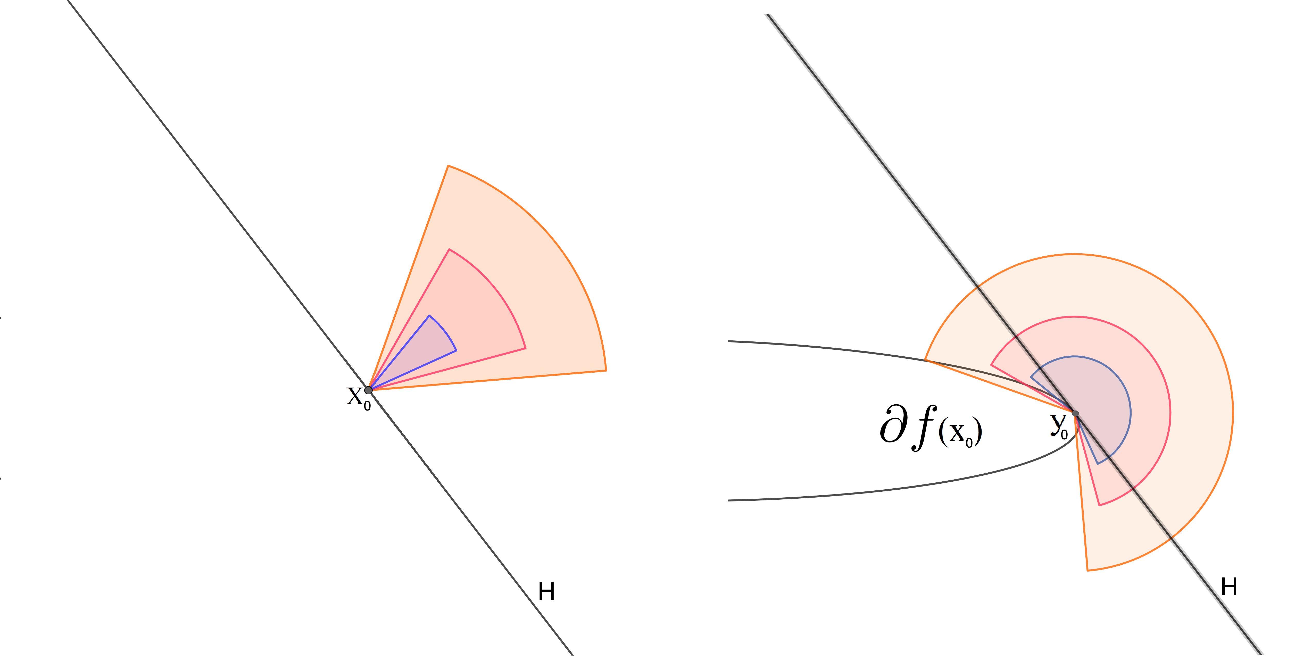
Figure 1: A visual illustration of the proof of Lemma 3.3. The subdifferential $\partial f$ maps each region of the figure on the left to the region of the same color on the right. In each region we can pick a point in $\mathcal{D}_{f\cap g}\coloneqq\{x\in\mathcal{H}:\ \partial f(x)\cap\partial g(x)\neq\emptyset\}$, hence create a sequence $x_{n}\to x_{0}$ with $\{x_{n}\}_{n\in\mathbb{N}}\subset\mathcal{D}_{f\cap g}$. Then the only possible limit for $\{y_{n}\}_{n\in\mathbb{N}}$ where $y_{n}\in\partial f(x_{n})\cap\partial g(x_{n})$ is $y_{0}$.

Lemma 3.3.

Let $f,g:\mathcal{H}\to(-\infty,+\infty]$ be proper l.s.c. convex functions such that the set

$$\mathcal{D}_{f\cap g}\coloneqq\{x\in\mathcal{H}:\ \partial f(x)\cap\partial g(x)\neq\emptyset\}$$

is dense in an open convex set $\mathcal{U}\subseteq\operatorname{int}(\operatorname{dom}(f))\cap\operatorname{int}(\operatorname{dom}(g))$. Then $\partial f=\partial g$ in $\mathcal{U}$.

Proof.

Suppose that there exists $x_{0}\in\mathcal{U}$ such that $\partial f(x_{0})\neq\partial g(x_{0})$. We will show that this assumption leads at a contradiction. The set $\partial f(x_{0})$ is convex and weakly compact (Bauschke and Combettes, 2011, Proposition 16.14) so that, via the Lindenstrauss theorem (see Lindenstrauss (1963, Theorem 4)), $\partial f(x_{0})$ is the closure of the convex hull of the set $S(x_{0})$ of its exposed points. That is, for any $y_{0}\in S(x_{0})$, there exists a supporting hyperplane $H\coloneqq\{z\in\mathcal{H}:\langle z,b\rangle+a=0\}$ such that

$$\partial f(x_{0})\cap H=\{y_{0}\}\quad\mbox{while}\quad\partial f(x_{0})\subseteq H^{-},$$

where $H^{-}\coloneqq\{z\in\mathcal{H}:\langle z,b\rangle+a\leq 0\}$; see the visual illustration provided in Figure 1. This implies that

$$\partial f(x_{0})\cap H^{+}=\partial f(x_{0})\cap\left((\mathcal{H}\setminus H^{-})\cup H\right)=\{y_{0}\},$$ (24)

where $H^{+}\coloneqq\{z\in\mathcal{H}:\langle z,b\rangle+a\geq 0\}$.

Without loss of generality, we can assume $x_{0}=y_{0}=0$, $\|b\|=1$, and $a=0$ (this can be achieved by redefining $f$ as in (17)). Denote by $\pi$ be the orthogonal projection to the space $\{\lambda\,b:\ \lambda\in\mathbb{R}\}^{\bot}$. Thus, for any $z\in\mathcal{H}$, we can write $z=\langle z,b\rangle b+\pi(z)$ where $\langle b,\pi(z)\rangle=0$. Consider the open convex truncated cone (see Figure 1 for an illustration)

$$C_{n}\coloneqq\left\{z\in\mathcal{H}:{n}^{-1}\langle z,b\rangle>\|\pi(z)\|\right\}\cap\mathcal{B}(0,\ {n}^{-1})\cap\mathcal{U}.$$

Let $\{x_{n}\}_{n\geq 1}\subseteq\operatorname{dom}(f)\cap\operatorname{dom}(g)$ be a sequence such that $x_{n}\in C_{n}$ for all $n\in\mathbb{N}$.Clearly, $x_{n}\to 0\equiv x_{0}$. However, by strong-to-weak continuity of the subdifferential (see part $(i)$ of Lemma 2.1), any sequence $y_{n}\in\partial f(x_{n})\cap\partial g(x_{n})$ converges weakly (possibly along subsequences) tosome $u\in\partial f(x_{0})\cap\partial g(x_{0})$. Let us now show that $u=y_{0}=0$. To do so, observe that, by cyclical monotonicity,

$$0\leq\langle x_{n}-x_{0},y_{n}-y_{0}\rangle=\langle x_{n},y_{n}\rangle\langle\pi(x_{n}),\pi(y_{n})\rangle+\langle x_{n},b\rangle\langle b,y_{n}\rangle\leq\|\pi(x_{n})\|\|\pi(y_{n})\|+\langle x_{n},b\rangle\langle b,y_{n}\rangle.$$

Since $x_{n}\in C_{n}$,

$$\langle x_{n},b\rangle({n}^{-1}\|\pi(y_{n})\|+\langle b,y_{n}\rangle)>\|\pi(y_{n})\|\|\pi(z)\|+\langle x_{n},b\rangle\langle b,y_{n}\rangle\geq 0$$

with $\langle x_{n},b\rangle>0$, so that $y_{n}\in\{y\in\mathcal{H}:\ -{n}^{-1}\|\pi(y)\|\leq\langle y,b\rangle\}.$

Let us show that the weak limit $u$ of $\{y_{n}\}_{n\in\mathbb{N}}$ is such that $\langle u,b\rangle\geq 0$. Suppose therefore that $\langle u,b\rangle=-\delta<0$. Then, by the definition of the weak limit of $\{y_{n}\}$, we obtain $\langle y_{n},b\rangle\to-\delta$; also note that $\lim\sup\|\pi(y_{n})\|\leq\lim\sup\|y_{n}\|<\infty$ (see e.g., Brezis (2010, Proposition 3.13 (iii))). We also know that $-{n}^{-1}\|\pi(y_{n})\|\leq\langle y_{n},b\rangle$, where taking limits yields the contradiction $0\leq-\delta$. Hence, $\langle u,b\rangle\geq 0$.

As a consequence, $u\in\partial f(x_{0})\cap\partial g(x_{0})\cap H^{+}$ where $H^{+}\coloneqq\{z:\langle z,b\rangle\geq 0\}$. However, in view of (24), $y_{0}$ is the only point in $\partial f(x_{0})\cap H^{+}$, so that $y_{0}=u$. This means that any $y_{0}$ belonging to $S(x_{0})$ (the set extreme points of $\partial f(x_{0})$) also belongs to $\partial g(x_{0})$. Hence, $S(x_{0})\subseteq\partial g(x_{0})$. Since $\partial g(x_{0})$ is convex and weakly compact, $\partial f(x_{0})\subseteq\partial g(x_{0})$. The converse follows by noting that $f$ and $g$ are playing fully symmetric roles. Thus we obtain that $\partial f(x_{0})=\partial g(x_{0})$, which yields the contradiction. The claim follows. ∎

Proof of Theorem 3.2.

The proof of Theorem 3.2 is similar to that of del Barrio et al. (2021b, Theorem 4.5) (see also González-Delgado et al. (2021) and del Barrio and Loubes (2019)) details therefore are skipped and only a brief outline of the proof is given.

The proof proceeds via an application of the Efron-Stein inequality to the random variable

$$R_{n}\coloneqq\mathcal{T}_{2}({\rm P}_{n},{\rm Q})-\int\psi(x)d{\rm P}_{n}(x).$$

Defining independent copies $X^{\prime}_{1},\ldots,X^{\prime}_{n}$ of the random variables $X_{1},\ldots,X_{n}$, denote by ${\rm P}_{n}^{(i)}$ the empirical measure on $(X_{1},\ldots,X_{i-1},X^{\prime}_{i},X_{i+1},\ldots,X_{n})$ and by $R_{n}^{(i)}$ the version of $R_{n}$ computed from ${\rm P}_{n}^{(i)}$ instead of ${\rm P}_{n}$. The proof consists in showing that the sequence $n(R_{n}-R_{n}^{(i)})$ converges almost surely to $0$ while $n^{2}\mathbb{E}[(R_{n}-R_{n}^{(i)})^{2}]$ is bounded by some constant $M$. This latter claim is a consequence of the finite fourth-order moment assumptions on ${\rm P}$ and ${\rm Q}$ while the first one (see Eq. (6.2) in del Barrio et al. (2021b)) results from the stability of the potentials in Theorem 3.1 $(ii)$—provided, however, that it holds true in this context. Assuming that it does, it follows from the Banach-Alaoglu theorem (see e.g., Brezis (2010, Theorem 3.16)) and the Banach-Saks property (see e.g., Brezis (2010, Exercise 5.24)) that there exists a subsequence of $\{n|R_{n}-R_{n}^{(i)}|\}_{n\in\mathbb{N}}$ the Cesàro mean of which converges to $0$ in $L^{2}(\mathbb{P})$. The same property holds for the Cesàro means of subsequences of $\{\sqrt{n}(R_{n}-\mathbb{E}R_{n})\}_{n\in\mathbb{N}}$. This implies (see p. 21 in del Barrio et al. (2021b)) that $\sqrt{n}\mathbb{E}|R_{n}-\mathbb{E}R_{n}|$ converges to zero and the central limit theorem holds.

The only ingredient missing in this sequence of arguments, thus, is the stability result of the potentials (Theorem 3.1-$(ii)$). The requirement here is the uniqueness (up to additive constants) of the population potential $\psi$, which we now establish: given two proper l.s.c.  convex functions $\psi$ and $f$ such that $\nabla\psi=\nabla f$ on a dense subset of $\operatorname{int}(\operatorname{supp}(\rm P))\subset\mathcal{H}$, let us show that $\psi$ and $f$ are equal (up to an additive constant) on $\operatorname{int}(\operatorname{supp}(\rm P))$.

Let $p\in\operatorname{int}(\operatorname{supp}(\rm P))$. Then there exists an open convex neighborhood $\mathcal{B}\subset\operatorname{int}(\operatorname{supp}(\rm P))$ of $p$. We have that $\nabla\psi=\nabla f$ on a dense subset $\mathcal{D}$ of $\mathcal{B}$. Lemma 3.3 thus implies that $\partial{\psi}=\partial{f}$ on $\mathcal{B}$. Let $\mathcal{B}^{\prime}$ be an open convex neighborhood of $p$ such that its topological closure $\overline{\mathcal{B}^{\prime}}$ is contained in $\mathcal{B}$. Define $s_{\overline{\mathcal{B}^{\prime}}}$ as the support function of $\overline{\mathcal{B}^{\prime}}$, i.e., $s_{\overline{\mathcal{B}^{\prime}}}(x)=0$ if $x\in\overline{\mathcal{B}^{\prime}}$ and $+\infty$ otherwise. Since $\partial\tilde{\psi}(h)=\partial\tilde{f}(h)=\emptyset$ for $h\in\mathcal{H}\setminus\overline{\mathcal{B}^{\prime}}$ and $\partial\tilde{\psi}(h)=\partial\tilde{f}(h)$ for $h\in\overline{\mathcal{B}^{\prime}}$, the functions $\tilde{\psi}\coloneqq\psi+s_{\overline{\mathcal{B}^{\prime}}}$ and $\tilde{f}\coloneqq f+s_{\overline{\mathcal{B}^{\prime}}}$ are proper l.s.c. convex functions with $\partial\tilde{\psi}=\partial\tilde{f}$ on $\mathcal{H}$ and $\nabla\tilde{\psi}=\nabla\tilde{f}$ in the dense subset $\tilde{\mathcal{D}}\coloneqq\mathcal{D}\cup(\mathcal{H}\setminus\overline{\mathcal{B}})$ of $\mathcal{H}$. Rockafellar (1970, Theorem B) then yields the existence of some $a=a_{p}\in\mathbb{R}$ such that $\tilde{\psi}=\tilde{f}+a$. Thus, $\psi=f+a$ on $\mathcal{B}^{\prime}$.

Up to this point, we have proven that, for all $p\in\mathcal{H}$, there exists a neighborhood $\mathcal{B}^{\prime}$ of $p$ and a constant $a=a_{p}\in\mathbb{R}$ such that $\psi=f+a$ on $\mathcal{B}^{\prime}$. Using a connectedness argument, let us show that this constant actually does not depend on $p$. The set $\Theta$ of all $x$ in $\operatorname{int}(\operatorname{supp}(\rm P))$ such that $\psi(x)=f(x)+a$ is open (i.e., each $q\in\Theta$ has a neighborhood where $\psi=f+a$) and non-empty (since $p\in\Theta$). Its complement is open, too (for each $q\not\in\Theta$ there exists a neighborhood of $q$ where $\psi=f+b$, with $b\neq a$, and this neighborhood obviously does not contain any element of $\Theta$). Since $\operatorname{int}(\operatorname{supp}(\rm P))$ is connected, $\Theta=\operatorname{int}(\operatorname{supp}(\rm P))$. This completes the proof of Theorem 3.2. ∎

3.3 Proof of Theorem 3.1

The proof of Theorem 3.1 relies on a series of lemmas. Some of these lemmas are self-contained “general” results; some others address the specific setting of Theorem 3.1.

Lemma 3.4.

Under the assumptions of Theorem 3.1, $\gamma_{n}\xrightarrow{w}\gamma$, where $\gamma\in\Pi({\rm P},{\rm Q})$ is the unique probability measure such that $\operatorname{supp}(\gamma)\subseteq\partial\psi$ for some l.s.c. convex function $\psi$.

Proof.

Lemma 2.4 implies that for any subsequence $\{\gamma_{n_{k}}\}_{k\in\mathbb{N}}$ there exists a further subse-quence $\{\gamma_{n_{k_{i}}}\}_{i\in\mathbb{N}}$ converging weakly to a probability measure $\gamma\in\Pi({\rm P},{\rm Q})$ such that $\operatorname{supp}(\gamma)\subseteq\partial\psi$ for some l.s.c. convex function $\psi$. Since $\partial\psi$ is ${\rm P}$-a.s. a singleton, it follows from Theorem 2.3 that $\gamma=({\rm Identity},\nabla\psi)\#{\rm P}$ is unique. Hence $\gamma_{n}\xrightarrow{w}\gamma$. ∎

In order to move from weak convergence of couplings to convergence of mappings, we use the set-topology of subdifferentials of the form $\partial\psi_{n}$ where $\psi_{n}$ denotes a sequence of convex functions defined over $\cal H$. Denoting by $\{A_{n}\}_{n\in\mathbb{N}}$ a sequence of subsets of a second countable topological space $\mathcal{Y}$, define the inner and outer limits of $\{A_{n}\}_{n\in\mathbb{N}}$ as

$$\operatorname{Liminn}_{n}^{\mathcal{Y}}A_{n}\coloneqq\{x\in\mathcal{Y}:\ \ \text{exists $\{x_{n}\}_{n\in\mathbb{N}}$ with $x_{n}\in A_{n}$ \text{such that} $x_{n}\xrightarrow{\mathcal{Y}}x$}\text{ as $n\to\infty$}\}\vspace{-4mm}$$

and

$$\hskip 21.33955pt\operatorname{Limout}_{n}^{\mathcal{Y}}A_{n}\coloneqq\{x\in\mathcal{Y}:\ \ \text{exists $\{x_{n_{k}}\}_{k\in\mathbb{N}}$ with $x_{n_{k}}\in A_{n_{k}}$ \text{such that} $x_{n_{k}}\xrightarrow{\mathcal{Y}}x$}\text{ as $k\to\infty$}\},$$

respectively. Here the convergence $x_{n}\xrightarrow{\mathcal{Y}}x$ is to be understood in the sense of the topology of $\mathcal{Y}$, i.e., for any neighborhood $\mathcal{U}_{x}$ of $x$, there exists $N_{\mathcal{U}_{x}}\in\mathbb{N}$ such that $x_{n}\in\mathcal{U}_{x}$, for all $n\geq N_{\mathcal{U}_{x}}$. The corresponding limit exists if and only if the inner and outer limits coincide, in which case we say that $\{A_{n}\}_{n\in\mathbb{N}}$ converges in the Painlevé-Kuratowski sense with respect to the topology of $\mathcal{Y}$. When the space $\mathcal{Y}$ is not second countable, the inner and outer limits are usually expressed in terms of nets instead of sequences. For ease of reference, we recall here a fundamental result on this type of set convergence, known in the literature as Mrówka’s theorem (see, e.g., Beer (1993, Theorem 5.2.12)).

Lemma 3.5 (Mrówka).

Let $\mathcal{Y}$ be a second countable topological space. Then, for any sequence $\{A_{n}\}_{n\in\mathbb{N}}$ of subsets of $\mathcal{Y}$, there exists a Painlevé-Kuratowski convergent subsequence $\{A_{n_{k}}\}_{k\in\mathbb{N}}$.

In particular, for $\mathcal{Y}=\mathcal{H}\times\mathcal{H}$, denote by

$$\operatorname{Limout}_{n}^{s-w}A_{n}\coloneqq\{(x,y)\in\mathcal{H}\times\mathcal{H}:\,\text{exists $(x_{n_{k}},y_{n_{k}})\in A_{n_{k}}$ \text{such that} $x_{n_{k}}\to x$ and $y_{n_{k}}\rightharpoonup y$}\}\vspace{-4mm}$$

and

$$\operatorname{Liminn}_{n}^{s-w}A_{n}\coloneqq\{(x,y)\in\mathcal{H}\times\mathcal{H}:\ \ \text{exists $(x_{n},y_{n})\in A_{n}$ \text{such that} $x_{n}\to x$ and $y_{n}\rightharpoonup y$}\},$$

respectively, the strong-to-weak outer limits and strong-to-weak inner limits of $\{A_{n}\}_{n\in\mathbb{N}}$. For sequences of subdifferentials of the form $\partial\psi_{n}$, when $\operatorname{Liminn}_{n}^{s-w}\partial\psi_{n}=\operatorname{Limout}_{n}^{s-w}\partial\psi_{n}$, we denote by $\operatorname{Lim}_{n}^{s-w}\partial\psi_{n}$ the strong-to-weak Painlevé-Kuratowski limit. Painlevé-Kuratowski limits are appropriate for sequences of cyclically monotone sets since, as the following result shows, they preserve that property.

Lemma 3.6.

Let $\{\Gamma_{n}\}_{n\in\mathbb{N}}$ be a sequence of cyclically monotone subsets of the product space $\mathcal{H}\times\mathcal{H}$. If $\Gamma^{s-w}\coloneqq\operatorname{Liminn}_{n}^{s-w}\Gamma_{n}\neq\emptyset$, then $\Gamma^{s-w}$ is also cyclically monotone.

Proof.

By definition, for each finite $N$-tuple $\{(x_{k},y_{k})\}_{k=1}^{N}\subseteq\Gamma^{s-w}$, there exists a sequenceof $N$-tuples $\{\{(x_{k}^{n},y_{k}^{n})\}_{k=1}^{N}\}_{n\in\mathbb{N}}$ with $\{(x_{k}^{n},y_{k}^{n})\}_{k=1}^{N}\subseteq\Gamma_{n}$ such that $x_{k}^{n}\rightarrow x_{k}$ and $y_{k}^{n}\rightharpoonup y_{k}$ as $n\to\infty$, for all $k=1,\dots,N$. For each $n\in\mathbb{N}$, cyclical monotonicity of $\Gamma_{n}$ implies

$$\sum_{k=1}^{N}\langle x_{k}^{n},y_{k+1}^{n}-y_{k}^{n}\rangle\leq 0.$$ (25)

Now, $\{\|y_{k+1}^{n}-y_{k}^{n}\|\}_{n\in{\mathbb{N}}}$ is bounded (e.g., Brezis (2010, Proposition 3.13 (iii))), so that

$$|\langle x_{k}^{n},y_{k+1}^{n}-y_{k}^{n}\rangle-\langle x_{k},y_{k+1}-y_{k}\rangle|=|\langle x_{k}^{n}-x_{k},y_{k+1}^{n}-y_{k}^{n}\rangle+\langle x_{k},y_{k+1}^{n}-y_{k}^{n}-(y_{k+1}-y_{k})\rangle|\\ \leq\|x_{k}^{n}-x_{k}\|\|y_{k+1}^{n}-y_{k}^{n}\|+|\langle x_{k},y_{k+1}^{n}-y_{k}^{n}-(y_{k+1}-y_{k})\rangle|\to 0.$$

Taking limits in (25) yields $\sum_{k=1}^{N}\langle x_{k},y_{k+1}-y_{k}\rangle\leq 0$. The claim follows. ∎

Let us now get back to the setting and the notation of Theorem 3.1. Observe that $\cal H\times\cal H$ with strong topologies on both sets is a separable metric space and hence is second countable (see Rudin (1953, Exercise 2.23)). The space $\mathcal{H}$ endowed with the weak topology, however, is not second countable (see Helmberg (2006, Corollary 1)), so that Mrówka’s theorem does not directly apply to $\operatorname{Lim}_{n}^{s-w}\partial\psi_{n}$ in the product space $\mathcal{H}\times\mathcal{H}$ when considering the strong topology in the first factor and the weak topology in the second one—see Beer (1993, Proposition 5.2.13) for a counter-example assuming the continuum hypothesis. However, consider the open ball $\mathcal{B}(0,{M})$ with radius $M$ centered at $0$, endowed with the metric structure $(\mathcal{B}(0,{M}),\|\cdot\|_{w})$, where

$$\|x\|_{w}\coloneqq\sum_{k\in\mathbb{N}}\frac{1}{2^{k}}\frac{|\langle x,e_{k}\rangle|}{1+|\langle x,e_{k}\rangle|}$$ (26)

with $\{e_{k}\}_{k\in\mathbb{N}}$ an orthonormal basis of $\cal H$. The norm (26) metrizes weak convergence in $\mathcal{B}(0,M)$, so that if $\bigcup_{n\in\mathbb{N},x\in K}\partial\psi_{n}(x)$ is a subset of $\mathcal{B}(0,M)$ — which holds by assumption — it is relatively compact in $(\mathcal{B}(0,M),\|\cdot\|_{w})$. Moreover, $(\mathcal{B}(0,M),\|\cdot\|_{w})$ is separable and, being metrizable, it is second countable, see Rudin (1953, Exercise 2.23). Mrówka’s theorem, thus, now applies.

Mrówka’s theorem (Lemma 3.5) implies that, given the sequence $\{\partial\psi_{n}\}_{n\in\mathbb{N}}$, there exists a subsequence $\{\partial\psi_{n_{k}}\}_{k\in\mathbb{N}}$ which converges, in the Painlevé-Kuratowski sense with respect to the strong-to-weak topology, to some $\Gamma^{\prime}$. But this limit may be the empty set, rendering the application of Mrówka’s theorem meaningless. The following Lemma shows that this is not the case for the sequence of subdifferentials. The strong-to-weak Painlevé-Kuratowski inner limit $\Gamma$ of $\{\partial\psi_{n}\}_{n\in\mathbb{N}}$ — hence, also the set $\Gamma^{\prime}\supseteq\Gamma$ — is non-empty and contains all the points of $\operatorname{supp}(\rm P)$ at which $\partial\psi$ is a singleton.

Lemma 3.7.

Under the assumptions of Theorem 3.1, the set $\operatorname{Liminn}_{s-w}\partial\psi_{n}$ in nonempty and, moreover, contains $\{(h,\nabla\psi(h)):\ h\in\operatorname{supp}(P)\cap\operatorname{dom}(\nabla\psi)\}$.

Proof.

Let $h\in\operatorname{supp}(P)\cap\operatorname{dom}(\nabla\psi)$ and let $y\coloneqq\nabla\psi(h)$. Denote by $\{\mathcal{U}_{y}^{m}\}_{m\in\mathbb{N}}$ a decreasing (i.e., $\mathcal{U}_{y}^{m}\subseteq\mathcal{U}_{y}^{m-1}$) countable sequence of neighborhoods (with respect to the strong topology) of $y$ such that $\bigcap_{m\in\mathbb{N}}\mathcal{U}_{y}^{m}=\{y\}$. Then, Bauschke and Combettes (2011, Theorem 21.22) entails the existence of a selection $\mathcal{Q}$ of $\partial\psi$ and a decreasing sequence of neighborhoods (with respect to the weak topology) $\{\mathcal{V}_{h}^{m}\}_{m\in\mathbb{N}}$ of $h$ such that $\bigcap_{m\in\mathbb{N}}\mathcal{V}_{h}^{m}=\{h\}$ and $\mathcal{Q}(\mathcal{V}_{h}^{m})\subseteq\mathcal{U}_{y}^{m}$ for all $m\in\mathbb{N}$. Since $\mathcal{V}_{h}^{m}$ has non-empty interior and $h\in\operatorname{supp}(P)$, and since $\gamma=({\rm Identity}\times\mathcal{Q}){\#}{\rm P}$, we have

$$\gamma(\mathcal{V}_{h}^{m}\times\mathcal{U}_{y}^{m})\geq\gamma(\mathcal{V}_{h}^{m}\times\mathcal{Q}(\mathcal{V}_{h}^{m}))=\mu(\mathcal{V}_{h}^{m})=:\delta_{m}>0.$$

Moreover, $\delta_{m}\to 0$ monotonically because $\bigcap_{m\in\mathbb{N}}\mathcal{V}_{h}^{m}=\{h\}$ and $\mathcal{V}_{h}^{m}\subseteq\mathcal{V}_{h}^{m-1}$. Fix $m\in\mathbb{N}$: since $\gamma_{n}$ converges weakly to $\gamma=({\rm Identity}\times\mathcal{Q}){\#}{\rm P}$, the Portmanteau theorem yields

$$\lim\inf_{n}\gamma_{n}(\mathcal{V}_{h}^{m}\times\mathcal{U}_{y}^{m})\geq\delta_{m},$$

so that there exists $N_{m}\in\mathbb{N}$ and a sequence $(h_{n},y_{n})$ such that

$$(h_{n},y_{n})\in(\mathcal{V}_{h}^{m}\times\mathcal{U}_{y}^{m})\cap\operatorname{supp}(\gamma_{n})$$

for all $n\geq N_{m}$. By definition of $\gamma_{n}$, there exists $(h_{n},y_{n})\in\partial\psi_{n}$ such that $h_{n}\in\mathcal{V}_{h}^{m}$ and $y_{n}\in~{}\!\mathcal{U}_{y}^{m}$. Letting $m\to~{}\!\infty$ yields a sequence $\{(h_{n},y_{n})\}_{n\in\mathbb{N}}$ with $(h_{n},y_{n})\in\partial\psi_{n}$, $h_{n}\longrightarrow h$, and $y_{n}\rightharpoonup~{}\!\nabla\psi(h)$, which completes the proof.∎

Lemma 3.6 implies that, in the context of Theorem 3.1, for any subsequence $\{n_{k}\}_{k\in\mathbb{N}}$, the limiting sets $\Gamma\coloneqq\operatorname{Liminn}_{n}^{s-w}\partial\psi_{n}$ and $\Gamma^{\prime}\coloneqq~{}\!\operatorname{Lim}_{k}^{s-w}\partial\psi_{n_{k}}$ both are cyclically monotone. As a consequence, there exists a convex function $\rho$ such that $\Gamma\subseteq\Gamma^{\prime}\subseteq\partial\rho$ (see Rockafellar (1970, Theorem B)). In view of Lemma 3.7, we have, still in the setting of Theorem 3.1, $(h,\nabla\psi(h))\in~{}\!\partial\rho$ for any $h\in\operatorname{supp}(P)\cap\operatorname{dom}(\nabla\psi)$. Since this set is dense in $\operatorname{supp}({\rm P})$ (see Bauschke and Combettes (2011, Theorem 21.22)), Lemma 3.3 entails $\partial\rho=\partial\psi$ in $\operatorname{int}\operatorname{supp}(\rm P)$, so that $\Gamma\subseteq\Gamma^{\prime}\subseteq\partial\psi$. This constitutes a fundamental difference with the finite-dimensional case. In Euclidean spaces, indeed, the limits of maximal monotone operators (subdifferentials of proper l.s.c. convex functions) is automatically maximal monotone (see e.g.  Adly et al. (2022)) and, instead of $\Gamma\subseteq\Gamma^{\prime}\subseteq\partial\psi$, it holds that $\Gamma=\Gamma^{\prime}=\partial\psi$. In the infinite-dimensional case, with the notation of Theorem 3.1, we thus have the following property.

Lemma 3.8.

Under the assumptions of Theorem 3.1,

1. for any $x\in\operatorname{dom}(\nabla\psi)\cap\,\operatorname{int}(\operatorname{supp}(\rm P))$, there exists a sequence $\{(x_{n},y_{n})\}_{n\geq 1}$ such that $x_{n}\to x$ and $y_{n}\rightharpoonup\nabla\psi(x)$ with $y_{n}\in\partial\psi(x_{n})$ for $n$ large enough;

2. for any sequence $\{(x_{n},y_{n})\}$ (or subsequence thereof) such that $x_{n}\to x\in\operatorname{int}(\operatorname{supp}(\rm P))$ and $y_{n}\rightharpoonup y$, with $y_{n}\in\partial\psi(x_{n})$ for $n$ large enough, $y\in\partial\psi(x)$.

We are now ready for the proof of Theorem 3.1.

Proof of Theorem 3.1.

First consider parts $(i)$ and $(iii)$. Set $h\in\mathcal{H}$ and suppose that

$$\liminf_{n\to\infty}\sup_{(x,y)\in\partial\psi_{n},\,x\in K}|\langle y-\nabla\psi(x),h\rangle|>\epsilon$$

for some $K\subseteq\operatorname{dom}(\nabla\psi)\cap\operatorname{int}(\operatorname{supp}(P))$: that implies the existence of sequences $\{x_{n_{k}}\}_{k\in\mathbb{N}}\subseteq K$ and $\{y_{n_{k}}\}_{k\in\mathbb{N}}\subseteq\mathcal{H}$ with $y_{n_{k}}\in\partial\psi_{n_{k}}(x_{n_{k}})$ such that, for all $k\geq 1$,

$$|\langle y_{n_{k}}-\nabla\psi(x_{n_{k}}),h\rangle|>\epsilon.$$ (27)

Since (by assumption) $\bigcup_{n\geq N_{0},x\in K}\partial\psi_{n}(x)$ is contained in the ball $\mathcal{B}(0,M)$, there exist (by the Banach-Alaoglu theorem; see e.g., Brezis (2010, Theorem 3.16)) a weak limit $y$ of the subsequence $\{y_{n_{k_{i}}}\}_{i\in\mathbb{N}}$ and (by the strong compactness of $K$) a strong limit $x$ of the subse-quence $\{x_{n_{k_{i}}}\}_{k\in\mathbb{N}}$. The limit $(x,y)$ belongs to the set $\operatorname{Liminn}_{i}^{s-w}\partial\psi_{n_{k_{i}}}$, hence, via Lemma 3.8, the only possible value of $(x,y)$ is $(x,\nabla\psi(x))$. This yields a contradiction to (27) and proves part $(i)$ of the theorem, of which part $(iii)$ is a direct consequence.

Turning to part $(ii)$, let $K$ be an arbitrary convex strongly compact subset of $\operatorname{supp}({\rm P})$. Starting from $K_{0}\coloneqq K$, one can create an increasing sequence $\{K_{i}\}_{i=0}^{\infty}$ of strongly compact convex sets such that ${\rm P}(\mathcal{H}\setminus K_{i})\leq\frac{1}{2^{i}}$. Let $\mathbb{K}\coloneqq\bigcup_{i\in\mathbb{N}}K_{i}$. The functions $\psi_{n}$ can be extended to be continuous on $\mathcal{H}$ in view of the fact that $\bigcup_{x\in\mathcal{H}}\partial\psi_{n}(x)\subset\mathcal{B}(0,M)$ (see e.g., (15)). Let $\mathcal{C}(\mathbb{K})$ denote the space of bounded continuous functions endowed with the metric

$$\|f\|_{\mathbb{K}}\coloneqq\sum_{j=0}^{\infty}\frac{\|f\|_{K_{j}}}{(\operatorname{diam}(K_{j})+1)^{2j}}$$

where $\|f\|_{K_{j}}\coloneqq{\sup_{x\in K_{j}}|f(x)|}$ and $\operatorname{diam}(K)\coloneqq\sup_{x,y\in K}\|x-y\|$. Observe that $f_{n}\to f$ in $\mathcal{C}(\mathbb{K})$ if and only if $f_{n}\to f$ uniformly in $K_{i}$ for all $i\in\mathbb{N}$. Since $\psi$, in part $(ii)$ of the theorem, is unique up to additive constants only, we can set $\psi_{n}(x_{0})=\psi(x_{0})=0$ for some $x_{0}\in{\rm supp}({\rm P})$. Note that, for any $x^{1},x^{2}\in K_{0}$ and $y_{n}^{1}\in\partial\psi_{n}(x^{1})$, $y_{n}^{2}\in\partial\psi_{n}(x^{2})$, the inequalities

$$\psi_{n}(x^{1})-\psi_{n}(x^{2})\leq\langle y_{n}^{1},x^{1}-x^{2}\rangle\quad\text{and}\quad\psi_{n}(x^{1})-\psi_{n}(x^{2})\geq\langle y_{n}^{2},x^{1}-x^{2}\rangle,$$ (28)

along with the assumption of bounded support, imply $|\psi_{n}(x^{1})-\psi_{n}(x^{2})|\leq M\|x^{1}-x^{2}\|$ for $n$ large enough. Then, the Arzelà-Ascoli theorem implies the uniform convergence of $\psi_{n}$ (along a subsequence $\{n^{0}_{k}\}_{k\in\mathbb{N}}$) to a function $\rho_{0}$ in $K_{0}$. Set $n_{0}\in\mathbb{N}$ such that $\|\rho_{0}-{\psi_{n_{0}}}\|_{K_{0}}\leq{1}/{2^{0}=1}$. We construct a general $\rho$ by using a diagonal argument: for $K_{1}$, there exists a subse-quence $\{n^{1}_{k}\}_{k\in\mathbb{N}}$ of $\{n^{0}_{k}\}_{k\in\mathbb{N}}$ such that $\psi_{n^{1}_{k}}$ converges uniformly in $K_{1}$ to a function $\rho_{1}$. Set $n_{1}\in\mathbb{N}$ such that $\|\rho_{1}-\psi_{n_{1}}\|_{K_{1}}\leq{1}/{2^{1}}=1/2$. Note that $\rho_{1}$ agrees with $\rho_{0}$ in $K_{0}$. Continuing in this fashion for $j=1,2,\ldots$, define $\rho_{j}$ on $K_{j}$, which agrees with $\rho_{i}$ on $K_{i}$ for $i<j$ with

$$\|\rho_{j}-\psi_{n_{j}}\|_{K_{j}}\leq\frac{1}{2^{j}}.$$ (29)

This iterative construction yields $\rho$ as the unique function in $\mathbb{K}$ which agrees with $\rho_{i}$ in $K_{i}$ for all $i\in{\mathbb{N}}$ and a sequence $\{n_{i}\}_{i\in\mathbb{N}}$ such that

$$\|\psi_{n_{i}}-\rho\|_{\mathbb{K}}\leq\frac{C}{2^{i}}+\sum_{j=n_{i}}^{\infty}\frac{\|\rho_{j}\|_{K_{j}}\|\psi_{n_{i}}\|_{K_{j}}}{(\operatorname{diam}(K_{j})+1)^{2j}}$$

where $C\coloneqq\sum_{j=0}^{\infty}{1}/{(\operatorname{diam}(K_{j})+1)^{2j}}<\infty$. Since

$$\|\rho_{j}\|_{K_{j}}\leq\|\psi_{n_{j}}\|_{K_{j}}+{1}/{2^{j}}\leq M\operatorname{diam}(K_{j})+{1}/{2^{j}},$$

the rest $\sum_{j=n_{i}}^{\infty}{\|\rho_{j}\|_{K_{j}}\|\psi_{n_{i}}\|_{K_{j}}}/{(\operatorname{diam}(K_{j})+1)^{2j}}$ of the series tends to zero as $i\to\infty$. As a consequence, $\|\psi_{n_{i}}-\rho\|_{\mathbb{K}}\to 0$ as $i\to\infty$. We claim that this limit $\rho$ is convex and continuous in $\mathbb{K}$. To prove convexity, set $t\in(0,1)$, $(x,y)\in\mathbb{K}^{2}$, and take limits (as $i\to\infty$) in

$$\psi_{n_{i}}(tx+(1-t)y)\leq t\psi_{n_{i}}(x)+(1-t)\psi_{n_{i}}(y).$$

To prove continuity in $\mathbb{K}$, set $(x^{1},x^{2})\in\mathbb{K}^{2}$. There exists some $K_{j}$ such that $x^{1}$ and $x^{2}$ both lie in $K_{\ell}$ for $\ell\geq j$. Since $|\psi_{n_{i}}(x^{1})-\psi_{n_{i}}(x^{2})|\leq M\|x^{1}-x^{2}\|$ and $\|\psi_{n_{i}}-\rho\|_{K_{j}}\to 0$, we conclude that

$$|\rho(x^{1})-\rho(x^{2})|\leq M\|x^{1}-x^{2}\|$$

by letting $i\to\infty$ in $|\rho(x^{1})-\rho(x^{2})|\leq 2\|\rho-\psi_{n_{i}}\|_{K_{j}}+|\psi_{n_{i}}(x^{1})-\psi_{n_{i}}(x^{2})|.$ Set $(i,j)\in\mathbb{N}^{2}$ and characterize the measure $\gamma_{n_{i}}^{K_{j}}$ by imposing $\int f(x,y)d\gamma_{n_{i}}^{K_{j}}(x,y)=\int\mathbb{I}_{K_{j}}(x)f(x,y)d\gamma_{n_{i}}(x,y)$ (where $\mathbb{I}_{K_{j}}$ denotes the indicator function of the set $K_{j}$) for any continuous boundedfunction $f:\mathcal{H}\times\mathcal{H}\to\mathbb{R}$. Denote by ${\rm P}_{n_{i}}^{K_{j}}$ and ${\rm Q}_{n_{i}}^{K_{j}}$ its marginals. Since $\operatorname{supp}(\gamma_{n_{i}})$ is cyclically monotone, $\operatorname{supp}(\gamma_{n_{i}}^{K_{j}})$ is cyclically monotone as well. The ‘truncated’ conjugate function

$$\psi^{*}_{n_{i},K_{j}}(y)\coloneqq\sup_{x\in K_{j}}\{\langle x,y\rangle-\psi_{n_{i}}(x)\},\qquad\;\;y\in\mathcal{H}$$

satisfies

$$\psi_{n_{i}}(x)+\psi^{*}_{n_{i},K_{j}}(y)=\langle x,y\rangle\quad\text{for $\gamma_{n_{i}}^{K_{j}}$-almost all~{}$(x,y)$}.$$ (30)

As $i\to+\infty$ with $j$ fixed, $\gamma_{n_{i}}^{K_{j}}$ tends weakly to the measure $\gamma^{K_{j}}$ characterized by

$$\int f(x,y)d\gamma^{K_{j}}(x,y)=\int\mathbb{I}_{K_{j}}(x)f(x,y)d\gamma(x,y)$$

for any continuous bounded function $f:\mathcal{H}\times\mathcal{H}\to\mathbb{R}$. Let us show that the truncated conjugate of $\rho$, namely,

$$\rho^{*}_{K_{j}}(y)\coloneqq\sup_{x\in K_{j}}\{\langle x,y\rangle-\rho(x)\}=\sup_{x\in K_{j}}\{\langle x,y\rangle-\rho_{j}(x)\}$$

is the uniform (in $\mathcal{H}$) limit of $\psi^{*}_{n_{i},K_{j}}$ as $i\to\infty$. To prove this claim, note that for all $y\in\mathcal{H}$ and all $i\geq j$,

$$|\psi^{*}_{n_{i},K_{j}}(y)-\rho^{*}_{K_{j}}(y)|\leq\|\rho_{j}-\psi_{n_{i}}\|_{K_{j}}=\|\rho_{i}-\psi_{n_{i}}\|_{K_{j}}\leq\|\rho_{i}-\psi_{n_{i}}\|_{K_{i}}\leq\frac{1}{2^{i}}\xrightarrow{i\to\infty}0,$$

where the last inequality holds by construction (see (29). As a consequence, from Markov’s inequality,

$${\rm Q}^{K_{i}}_{n_{i}}(\{y:\ |\rho_{K_{j}}^{*}(y)-\psi^{*}_{n_{i},K_{j}}(y)|>\delta\})\leq\frac{1}{2^{i}\delta}\to 0$$

as $i\to\infty$ with $j$ fixed, for all $\delta>0$. On the other hand, still using Markov’s inequality, we obtain

$${\rm P}_{n_{i}}^{K_{j}}(\{x:\ |\psi_{n_{i}}(x)-\rho(x)|>\delta\}) ={\rm P}_{n_{i}}(\{x:\ |\psi_{n_{i}}(x)-\rho_{i}(x)|>\delta\}\cap K_{j})\leq\frac{1}{2^{i}\delta},$$

which tends to zero as $i\to\infty$ with $j$ fixed. Then,

$$\gamma_{n_{i}}^{K_{j}}\big{(}\{(x,y):\ |\rho(x)+\rho_{K_{j}}^{*}(y)-(\psi_{n_{i}}(x)+\psi^{*}_{n_{i},K_{j}}(y))|>\delta\}\big{)}\to 0$$

as $i\to\infty$ so that, via (30),

$$\gamma_{n_{i}}^{K_{j}}(\{(x,y):\ |\langle x,y\rangle-(\rho(x)+\rho_{K_{j}}^{*}(y))|>\delta\})\to 0$$

as $i\to\infty$. Since (by the continuity of $\rho$ and $\rho_{K_{j}}^{*}$ in $K_{j}$ and $\mathcal{H}$, respectively) the set

$$\{(x,y)\in K_{j}\times\mathcal{H}:\ |\langle x,y\rangle-(\rho(x)+\rho_{K_{j}}^{*}(y))|>\delta\}$$

is open in $K_{j}\times\mathcal{H}$, the Portmanteau theorem yields

$$0=\liminf_{i}\gamma_{n_{i}}^{K_{j}}(\{(x,y):\ |\langle x,y\rangle-(\rho(x)+\rho_{K_{j}}^{*}(y))|>\delta\})\\ \geq\gamma^{K_{j}}(\{(x,y):\ |\langle x,y\rangle-(\rho(x)+\rho_{K_{j}}^{*}(y))|>\delta\}).$$

From this we conclude that $\gamma^{K_{j}}(\{(x,y):\ |\langle x,y\rangle-(\rho(x)+\rho_{K_{j}}^{*}(y))|>\delta\})=0$. Thus, on the one hand,

$$\langle x,y\rangle-(\rho_{i}(x)+\rho_{K_{j}}^{*}(y))=0,\quad\text{for ${\gamma}^{K_{j}}$-almost all $(x,y)$}$$ (31)

and, on the other hand,

$$\langle x,y\rangle-(\psi(x)+\psi^{*}(y))=0,\quad\text{for ${\gamma}^{K_{j}}$-almost all $(x,y)$}.$$ (32)

Theorem 2.3 applied to the marginals ${\rm P}^{K_{j}}$ and ${\rm Q}^{K_{j}}$ of ${\gamma}^{K_{j}}$ (rescaled in order to be probability measures) yields $\nabla\rho(x)=\nabla\psi(x)$ for ${\rm P}^{K_{j}}$-almost all $x$. That is, $\nabla\rho(x)=\nabla\psi(x)$ for ${\rm P}$-almost all $x\in K_{j}$. As a consequence,

$${\rm P}(\{x\in\mathcal{H}:\ \nabla\rho(x)\neq\nabla\psi(x)\}) \leq{\rm P}(\{x\in\mathcal{H}:\ \nabla\rho(x)\neq\nabla\psi(x)\}\cap K_{j})+{\rm P}(\mathcal{H}\setminus K_{j})$$

$$={\rm P}(\mathcal{H}\setminus K_{j})\leq\frac{1}{2^{j}}.$$

Letting $j\to\infty$, we obtain ${\rm P}(\{x\in\mathcal{H}:\ \nabla\rho(x)=\nabla\psi(x)\})=1$. Then, by the assumed uniqueness, there exists $a\in\mathbb{R}$ such that $\rho=\psi+a$ $\rm P$-a.s. Such an $a$ must be zero due to the fact that $\rho(x_{0})=\lim_{i\to\infty}\psi_{n_{i}}(x_{0})=\psi(x_{0})$.

To conclude, let us show that $\rho(x)=\psi(x)$ for all $x\in K$. Assume that $\rho(x_{1})\neq\psi(x_{1})$ for some $x_{1}\in K_{0}=K\subset\operatorname{supp}({\rm P})$. The continuity of $\rho-\psi$ in $\mathbb{K}$ implies that $\rho(x)\neq\psi(x)$ for all $x\in\mathcal{B}(x_{1},\epsilon)\cap\mathbb{K}$ with $\epsilon>0$ small enough. This, however, cannot be since ${\rm P}(\mathcal{B}(x_{1},\epsilon)\cap\mathbb{K})>0$. Hence, $\rho(x)=\psi(x)$ for all $x\in K$, as was to be shown. ∎

Funding

The research of Alberto González-Sanz is partially supported by grant PID2021-128314NB-I00 funded by MCIN/AEI/ 10.13039/501100011033/FEDER, UE and by the AI Interdisciplinary Institute ANITI, which is funded by the French “investing for the Future – PIA3" program under the Grant agreement ANR-19-PI3A-0004. The research of Marc Hallin is supported by the Czech Science Foundation grant GAČR22036365, and the research of Bodhisattva Sen is supported by NSF grant DMS-2015376.

References

- Adly et al. (2022) Adly, S., H. Attouch, and R. T. Rockafellar (2022, June). Preservation or not of the maximally monotone property by graph-convergence. HAL Preprint.
- Ambrosio et al. (2005) Ambrosio, L., N. Gigli, and G. Savare (2005). Gradient Flows in Metric Spaces and in the Space of Probability Measures. Birkhäuser Basel.
- Anderson and Klee, Jr. (1952) Anderson, R. D. and V. L. Klee, Jr. (1952). Convex functions and upper semi-continuous collections. Duke Mathematical Journal 19(2), 349 – 357.
- Bauschke and Combettes (2011) Bauschke, H. H. and P. L. Combettes (2011). Convex Analysis and Monotone Operator Theory in Hilbert Spaces. Springer.
- Beer (1993) Beer, G. (1993). Topologies on Closed and Closed Convex Sets. Springer Dordrecht.
- Bogachev (2008) Bogachev, V. (2008). Gaussian Measures. American Mathematical Society.
- Brenier (1991) Brenier, Y. (1991). Polar factorization and monotone rearrangement of vector-valued functions. Communications on Pure and Applied Mathematics 44(4), 375–417.
- Brezis (2010) Brezis, H. (2010). Functional Analysis, Sobolev Spaces and Partial Differential Equations. New York: Springer.
- Chakraborty and Chaudhuri (2014a) Chakraborty, A. and P. Chaudhuri (2014a). On data depth in infinite-dimensional spaces. Ann. Inst. Statist. Math. 66, 303–324.
- Chakraborty and Chaudhuri (2014b) Chakraborty, A. and P. Chaudhuri (2014b). The spatial distribution in infinite-dimensional spaces and related quantiles and depths. Ann. Statist. 42(3), 1203–1231.
- Chernozhukov et al. (2017) Chernozhukov, V., A. Galichon, M. Hallin, and M. Henry (2017). Monge-Kantorovich depth, quantiles, ranks and signs. Ann. Statist. 45, 223–256.
- Cordero-Erausquin and Figalli (2019) Cordero-Erausquin, D. and A. Figalli (2019). Regularity of monotone transport maps between unbounded domains. Discrete & Continuous Dynamical Systems 39, 7101–7112.
- Csörnyei (1999) Csörnyei, M. (1999). Aronszajn null and Gaussian null sets coincide. Israel Journal of Mathematics 111, 191–201.
- Cuesta-Albertos et al. (2006) Cuesta-Albertos, J. A., R. Fraiman, and T. Ransford (2006). Random projections and goodness-of-fit tests in infinite-dimensional spaces. Bull. Braz. Math. Soc. (N.S.) 37(4), 477–501.
- Cuesta-Albertos and Matrán (1989) Cuesta-Albertos, J. A. and C. Matrán (1989). Notes on the Wasserstein metric in Hilbert spaces. Annals of Probability 17, 1264–1276.
- Cuesta-Albertos et al. (1996) Cuesta-Albertos, J. A., C. Matrán-Bea, and A. Tuero-Diáz (1996). On lower bounds for the -Wasserstein metric in a Hilbert space. Journal of Theoretical Probability 9, 263–283.
- Deb and Sen (2023) Deb, N. and B. Sen (2023). Multivariate rank-based distribution-free nonparametric testing using measure transportation. J. Amer. Statist. Assoc. 118(541), 192–207.
- del Barrio and González-Sanz (2023) del Barrio, E. and A. González-Sanz (2023). Regularity of center-outward distribution functions in non-convex domains. arXiv:2303.16862.
- del Barrio et al. (2020) del Barrio, E., A. González-Sanz, and M. Hallin (2020). A note on the regularity of optimal-transport-based center-outward distribution and quantile functions. Journal of Multivariate Analysis 180, 104671.
- del Barrio et al. (2021a) del Barrio, E., A. González-Sanz, and J.-M. Loubes (2021a). A central limit theorem for semidiscrete Wasserstein distances. arXiv 2105.11721.
- del Barrio et al. (2021b) del Barrio, E., A. González-Sanz, and J.-M. Loubes (2021b). Central limit theorems for general transportation costs. To appear in Annales de l’Institut Henri Poincaré. Available as ArXiv:2102.06379.
- del Barrio et al. (2022) del Barrio, E., A. González-Sanz, and M. Hallin (2022). Nonparametric multiple-output center-outward quantile regression. arXiv: Probability.
- del Barrio and Loubes (2019) del Barrio, E. and J.-M. Loubes (2019). Central limit theorems for empirical transportation cost in general dimension. The Annals of Probability 47(2), 926 – 951.
- Edgar (1977) Edgar, G. A. (1977). Measurability in a Banach space. Indiana University Mathematics Journal 26(4), 663–677.
- Figalli (2017) Figalli, A. (2017). The Monge-Ampère Equation and Its Applications. Zurich: Zurich Lectures in Advanced Mathematics, European Mathematical Society (EMS).
- Figalli (2018) Figalli, A. (2018). On the continuity of center-outward distribution and quantile functions. Nonlinear Analysis 177, 413–421. Nonlinear PDEs and Geometric Function Theory, in honor of Carlo Sbordone on his 70th birthday.
- Gangbo and McCann (1996) Gangbo, W. and R. J. McCann (1996). The geometry of optimal transportation. Acta Mathematica 177(2), 113 – 161.
- Ghosal and Sen (2022) Ghosal, P. and B. Sen (2022). Multivariate ranks and quantiles using optimal transport: Consistency, rates and nonparametric testing. Ann. Statist. 50, 1012 – 1037.
- González-Delgado et al. (2021) González-Delgado, J., A. González-Sanz, J. Cortés, and P. Neuvial (2021). Two-sample goodness-of-fit tests on the flat torus based on Wasserstein distance and their relevance to structural biology. arXiv: Probability.
- Hallin (2022) Hallin, M. (2022). Measure transportation and statistical decision theory. Annual Review of Statistics and its Applications 9, 401–424.
- Hallin et al. (2021) Hallin, M., E. del Barrio, J. Cuesta-Albertos, and C. Matrán (2021). Distribution and quantile functions, ranks and signs in dimension d: A measure transportation approach. The Annals of Statistics 49(2), 1139 – 1165.
- Hallin et al. (2022) Hallin, M., D. Hlubinka, and Š. Hudecová (2022). Fully distribution-free center-outward rank tests for multiple-output regression and MANOVA. Journal of the American Statistical Association, in print. Available at arXiv:2007.15496v1.
- Hallin et al. (2022a) Hallin, M., D. La Vecchia, and H. Liu (2022a). Center-outward R-estimation for semiparametric VARMA models. J. Amer. Statist. Assoc., 117.
- Hallin et al. (2022b) Hallin, M., D. La Vecchia, and H. Liu (2022b). Rank-based testing for semiparametric VAR models: a measure transportation approach. Bernoulli, 925–938.
- Hallin and Liu (2022) Hallin, M. and H. Liu (2022). Center-outward rank- and sign-based VARMA portmanteau tests: Chitturi, Hosking, and Li–Mcleod revisited.
- Hallin and Mordant (2022) Hallin, M. and G. Mordant (2022). Center-outward multiple-output Lorenz curves and Gini indices: a measure transportation approach.
- Helmberg (2006) Helmberg, G. (2006). Curiosities concerning weak topology in Hilbert space. The American Mathematical Monthly 113(5), 447–452.
- Hiriart-Urruty (1980) Hiriart-Urruty, J.-B. (1980). Extension of Lipschitz functions. Journal of Mathematical Analysis and Applications 77(2), 539–554.
- Horváth and Kokoszka (2012) Horváth, L. and P. Kokoszka (2012). Inference for Functional Data with Applications. Springer Series in Statistics. Springer, New York.
- Hsing and Eubank (2015) Hsing, T. and R. Eubank (2015). Theoretical Foundations of Functional Data Analysis, with an Introduction to Linear Operators. Wiley Series in Probability and Statistics. John Wiley & Sons, Ltd., Chichester.
- Huang and Sen (2023) Huang, Z. and B. Sen (2023). Multivariate symmetry: Distribution-free testing via optimal transport. arXiv preprint arXiv:2305.01839.
- Hundrieser et al. (2022) Hundrieser, S., T. Staudt, and A. Munk (2022). Empirical optimal transport between different measures adapts to lower complexity. arXiv:2202.10434.
- Jayasumana et al. (2013) Jayasumana, S., M. Salzmann, H. Li, and M. Harandi (2013). A framework for shape analysis via Hilbert space embedding. In Proceedings of the IEEE International Conference on Computer Vision, pp. 1249–1256.
- Kokoszka and Reimherr (2017) Kokoszka, P. and M. Reimherr (2017). Introduction to Functional Data Analysis. Texts in Statistical Science Series. CRC Press, Boca Raton, FL.
- Lai et al. (2021) Lai, T., Z. Zhang, Y. Wang, and L. Kong (2021). Testing independence of functional variables by angle covariance. J. Multivariate Anal. 182, Paper No. 104711, 15.
- Lindenstrauss (1963) Lindenstrauss, J. (1963). On operators which attain their norm. Israel Journal of Mathematics 1, 139–148.
- Marron and Alonso (2014) Marron, J. S. and A. M. Alonso (2014). Overview of object oriented data analysis. Biom. J. 56(5), 732–753.
- McCann (1995) McCann, R. J. (1995). Existence and uniqueness of monotone measure-preserving maps. Duke Mathematical Journal 80(2), 309 – 323.
- Menafoglio and Petris (2016) Menafoglio, A. and G. Petris (2016). Kriging for Hilbert-space valued random fields: the operatorial point of view. J. Multivariate Anal. 146, 84–94.
- Rockafellar (1970) Rockafellar, R. T. (1970). On the maximal monotonicity of subdifferential mappings. Pacific Journal of Mathematics 33(1), 209 – 216.
- Rockafellar and Wets (2009) Rockafellar, R. T. and R. J.-B. Wets (2009). Variational Analysis. Springer Science & Business Media.
- Rudin (1953) Rudin, W. (1953). Principles of Mathematical Analysis. McGraw-Hill Book Company, Inc., New York-Toronto-London.
- Rudin (1990) Rudin, W. (1990). Functional Analysis. New York: McGraw-Hill.
- Rüschendorf and Rachev (1990) Rüschendorf, L. and S. T. Rachev (1990). A characterization of random variables with minimum L2-distance. J. Multivariate Anal. 32, 48–54.
- Segers (2022) Segers, J. (2022). Graphical and uniform consistency of estimated optimal transport plans. arXiv:2208.02508.
- Shapiro (1990) Shapiro, A. (1990). On concepts of directional differentiability. Journal of Optimization Theory and Applications 66, 477–487.
- Shi et al. (2021) Shi, H., M. Drton, M. Hallin, and F. Han (2021). Center-outward sign- and rank-based Quadrant, Spearman, and Kendall tests for multivariate independence.
- Shi et al. (2022) Shi, H., M. Hallin, M. Drton, and F. Han (2022). On universally consistent and fully distribution-free rank tests of vector independence. Ann. Statist., 50, 1933–1959.
- Small and McLeish (1994) Small, C. G. and D. L. McLeish (1994). Hilbert space Methods in Probability and Statistical Inference. Wiley Series in Probability and Mathematical Statistics. John Wiley & Sons, Inc., New York.
- Tukey (1975) Tukey, J. W. (1975). Mathematics and the picturing of data. Proceedings of the International Congress of Mathematicians, Vancouver, 1975 2, 523–531.
- Villani (2003) Villani, C. (2003). Topics in optimal transportation, Volume 58 of Graduate Studies in Mathematics. American Mathematical Society, Providence, RI.
- Villani (2009) Villani, C. (2009). Optimal transport, Volume 338 of Grundlehren der mathematischen Wissenschaften [Fundamental Principles of Mathematical Sciences]. Springer-Verlag, Berlin. Old and new.
- Weed and Bach (2019) Weed, J. and F. Bach (2019). Sharp asymptotic and finite-sample rates of convergence of empirical measures in Wasserstein distance. Bernoulli 25(4A), 2620–2648.
- Zajíček (1978) Zajíček, L. (1978). On the points of multivaluedness of metric projections in separable Banach spaces. Commentationes Mathematicae Universitatis Carolinae 019(3), 513–523.
- Zajíček (1979) Zajíček, L. (1979). On the differentiation of convex functions in finite- and infinite-dimensional spaces. Czechoslovak Mathematical Journal 29(3), 340–348.
- Zajíček (1983) Zajíček, L. (1983). Differentiability of the distance function and points of multi-valuedness of the metric projection in Banach space. Czechoslovak Mathematical Journal 33(2), 292–308.