Efficient and Deterministic Search Strategy Based on Residual Projections for Point Cloud Registration

Abstract

Estimating the rigid transformation between two LiDAR scans through putative 3D correspondences is a typical point cloud registration paradigm. Current 3D feature matching approaches commonly lead to numerous outlier correspondences, making outlier-robust registration techniques indispensable. Many recent studies have adopted the branch and bound (BnB) optimization framework to solve the correspondence-based point cloud registration problem globally and deterministically. Nonetheless, BnB-based methods are time-consuming to search the entire 6-dimensional parameter space, since their computational complexity is exponential to the dimension of the solution domain. In order to enhance algorithm efficiency, existing works attempt to decouple the 6 degrees of freedom (DOF) original problem into two 3-DOF sub-problems, thereby reducing the dimension of the parameter space. In contrast, our proposed approach introduces a novel pose decoupling strategy based on residual projections, effectively decomposing the raw problem into three 2-DOF rotation search sub-problems. Subsequently, we employ a novel BnB-based search method to solve these sub-problems, achieving efficient and deterministic registration. Furthermore, our method can be adapted to address the challenging problem of simultaneous pose and correspondence registration (SPCR). Through extensive experiments conducted on synthetic and real-world datasets, we demonstrate that our proposed method outperforms state-of-the-art methods in terms of efficiency, while simultaneously ensuring robustness.

1 Introduction

Rigid point cloud registration is a core and fundamental problem in the field of 3D vision and robotics with a wide range of applications, such as autonomous driving[1, 2], 3D reconstruction[3, 4], and simultaneous localization and mapping (SLAM)[5, 6, 7]. Given the source and target point clouds in different coordinate systems, it aims to estimate the 6 degrees of freedom (DOF) transformation in $\mathbb{SE}(3)$ to align the two point clouds best. The 6-DOF transformation includes both 3-DOF rotation in $\mathbb{SO}(3)$ and 3-DOF translation in $\mathbb{R}^{3}$.

Despite decades of research, rigid point could registration is still an active and challenging problem since it has chicken-and-egg property[8]. Specifically, the registration problem comprises two mutually interlocked sub-problems: pose and correspondence estimations. If one sub-problem is solved, another sub-problem will be solved accordingly. Commonly, existing registration methods are classified into two categories based on the requirement of correspondences or not, which are correspondence-based registration (e.g., fast global registration, FGR[9]) and simultaneous pose and correspondence registration (SPCR) (e.g., iterative closest point, ICP[10]). The widely used ICP is a local optimization method for SPCR, which means that it is highly dependent on the initialization of transformation and thus prone to fall into local minima, as shown in Fig. 1(d-2). The global methods for SPCR, however, deliver relatively low efficiency (e.g., globally optimal ICP, Go-ICP[11]), as shown in Fig. 1(d-3). Thus the correspondence-based registration approaches are gradually attracting attention since they are initialization-free and more efficient[9, 12]. In this paper, we focus on the correspondence-based registration problem, while, interestingly, our approach can also be extended to solve the challenging SPCR problem.

Correspondence-based (FPFH descriptor)
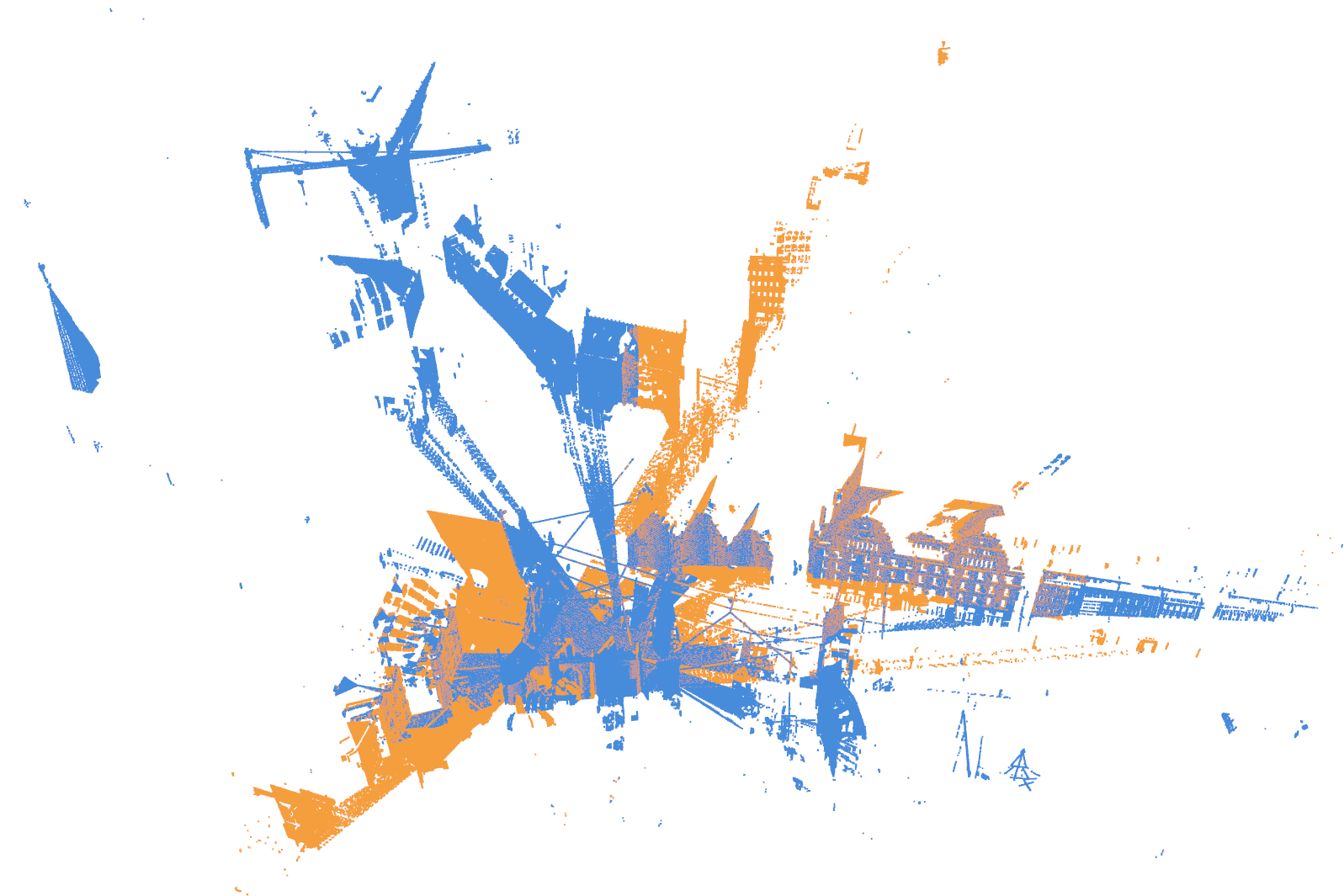
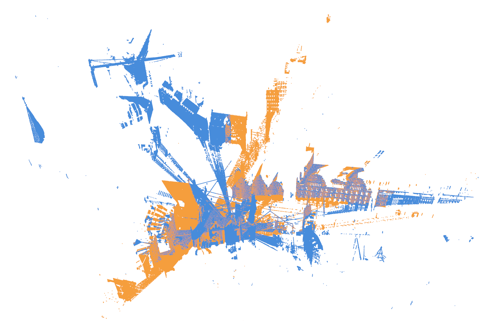
	(a-1) Initial ($94.20\%$ outlier)	(a-2) GORE[13]	(a-3) TEASER[12]	(a-4) Ours
	-	$E_{\bm{R}}=0.041\degree$	$E_{\bm{R}}=0.069\degree$	$E_{\bm{R}}=\textbf{0.004}\degree$
	-	$E_{\bm{t}}=0.055$\mathrm{m}$$	$E_{\bm{t}}=0.067$\mathrm{m}$$	$E_{\bm{t}}=\textbf{0.042}$\mathrm{m}$$
	-	${time}=403.1$s	${time}=1.357$s	${time}=\textbf{0.307}$s
Correspondence-based (FPFH descriptor)
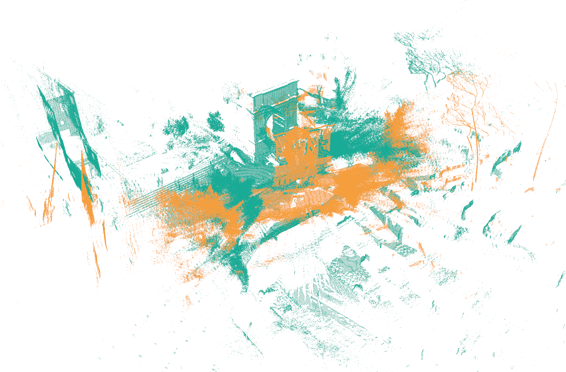
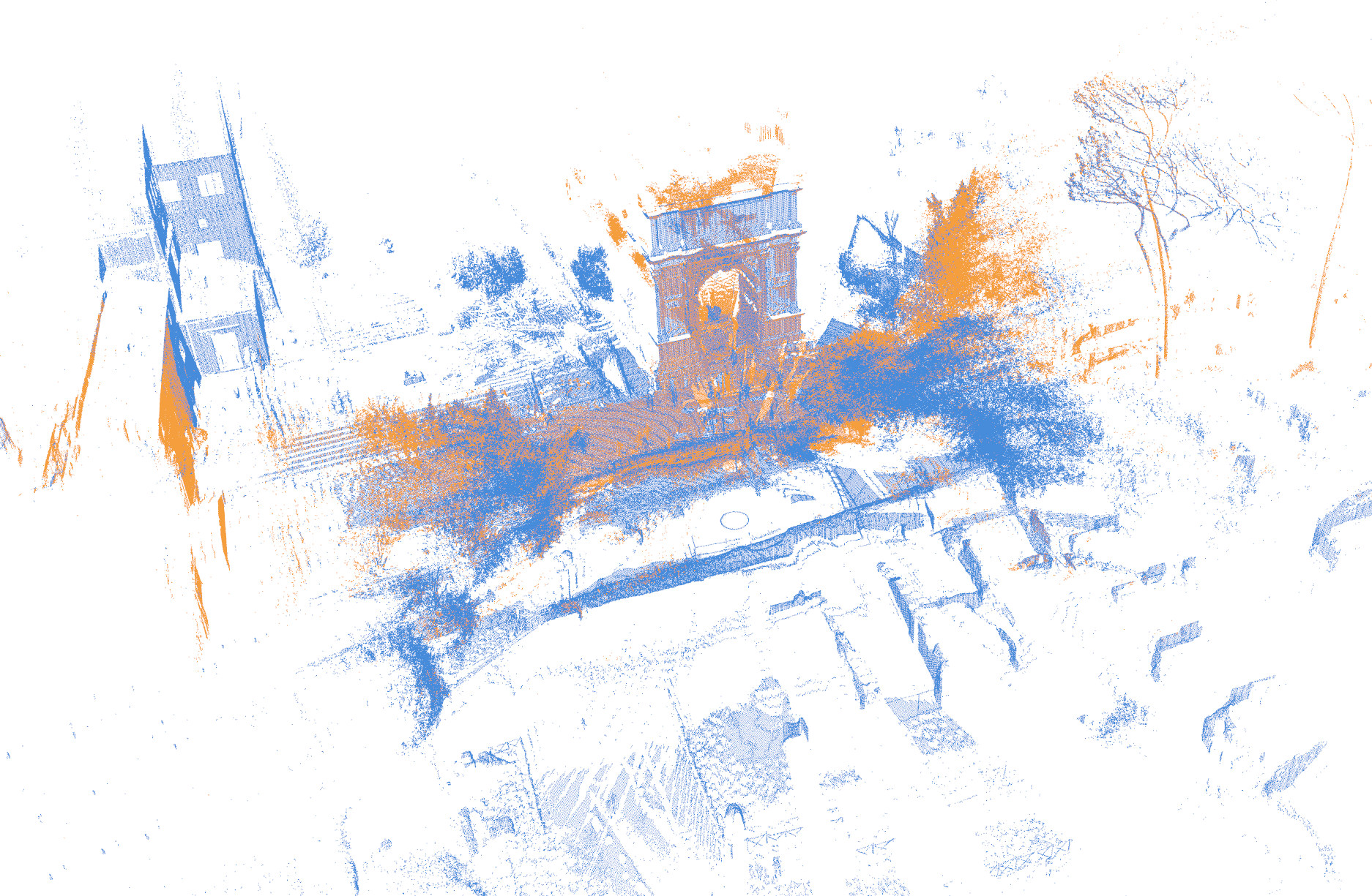
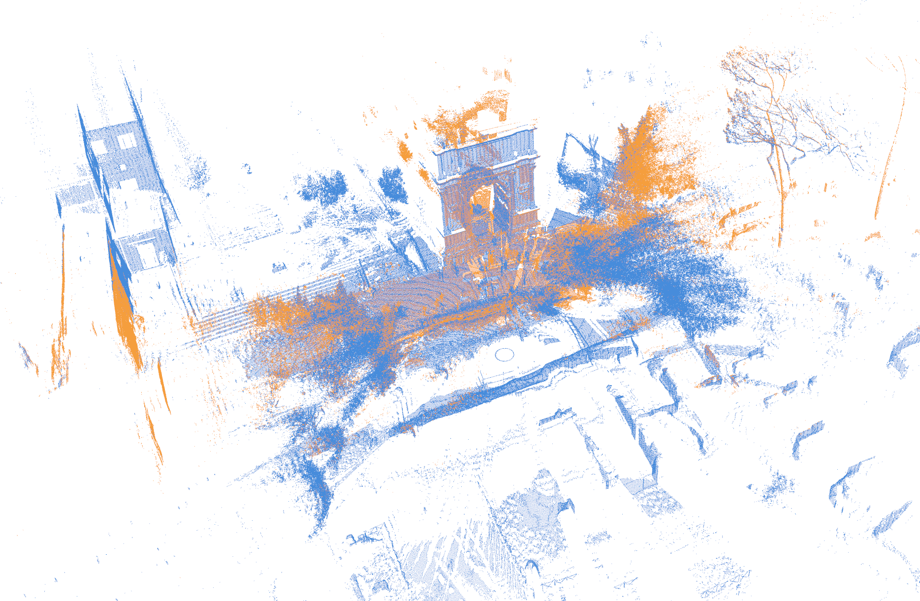
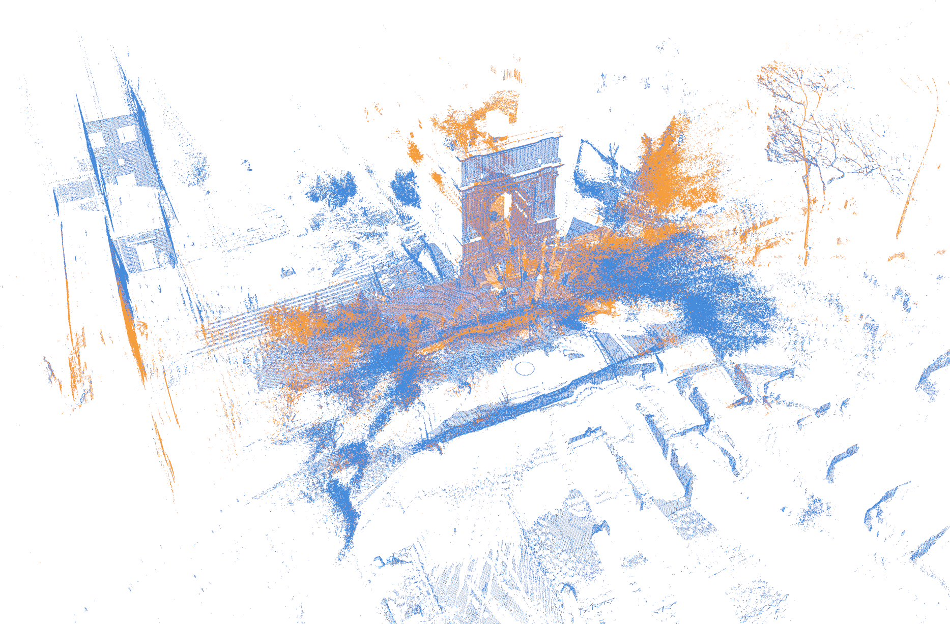
	(b-1) Initial ($98.45\%$ outlier)	(b-2) GORE[13]	(b-3) TEASER[12]	(b-4) Ours
	-	$E_{\bm{R}}=\textbf{0.055}\degree$	$E_{\bm{R}}=0.197\degree$	$E_{\bm{R}}=0.104\degree$
	-	$E_{\bm{t}}=\textbf{0.018}$\mathrm{m}$$	$E_{\bm{t}}=0.031$\mathrm{m}$$	$E_{\bm{t}}=\textbf{0.018}$\mathrm{m}$$
	-	${time}=687.7$s	${time}=5.917$s	${time}=\textbf{1.436}$s
Correspondence-based (FCGF descriptor)
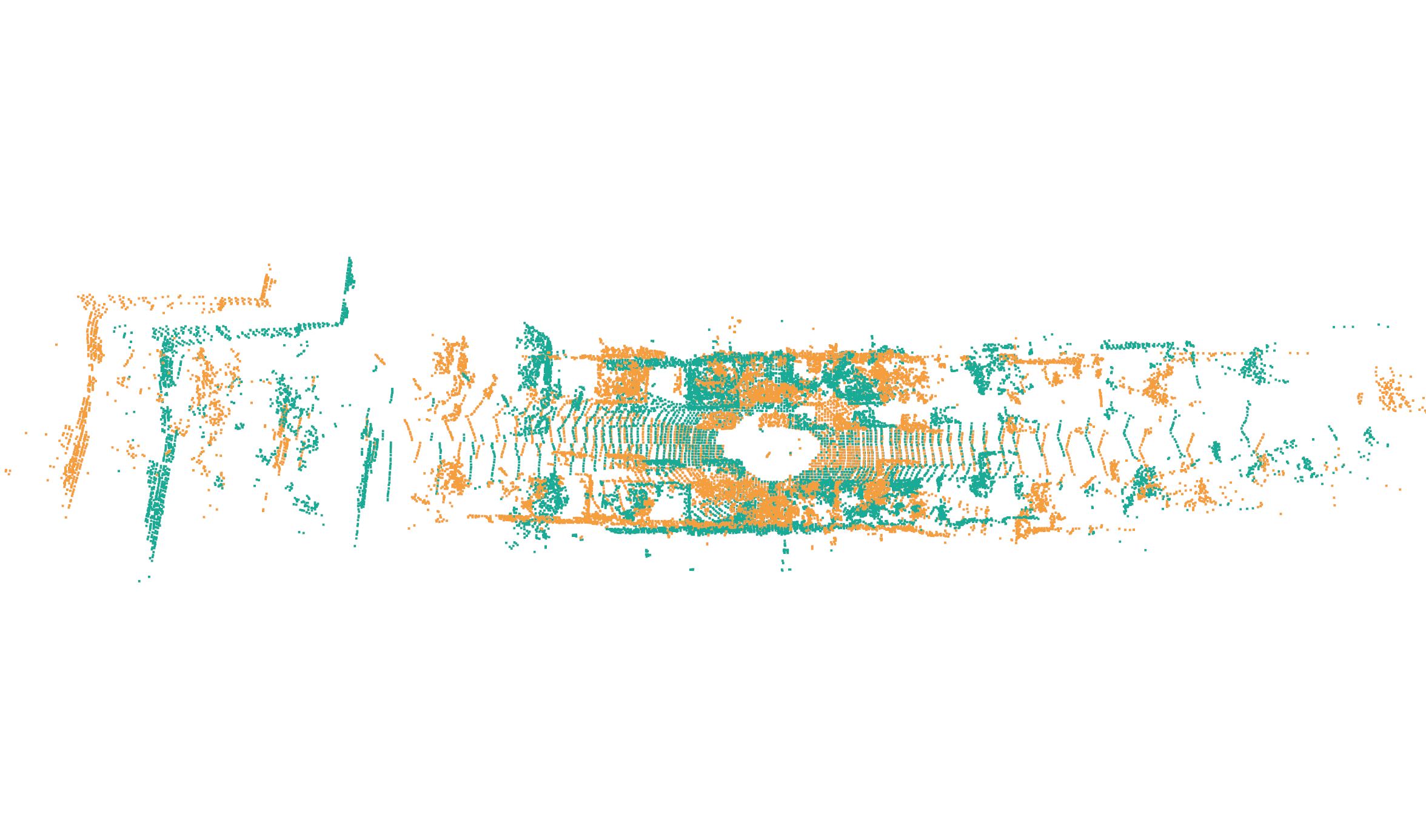
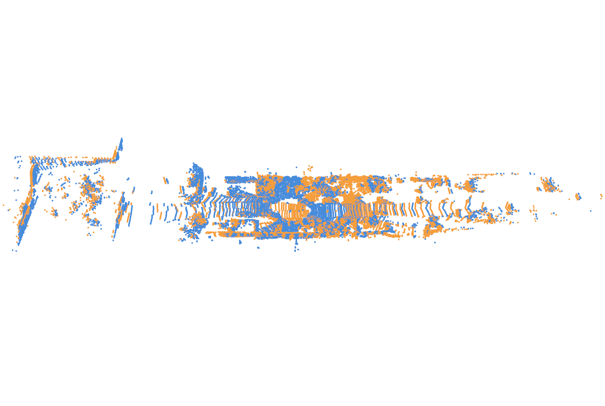
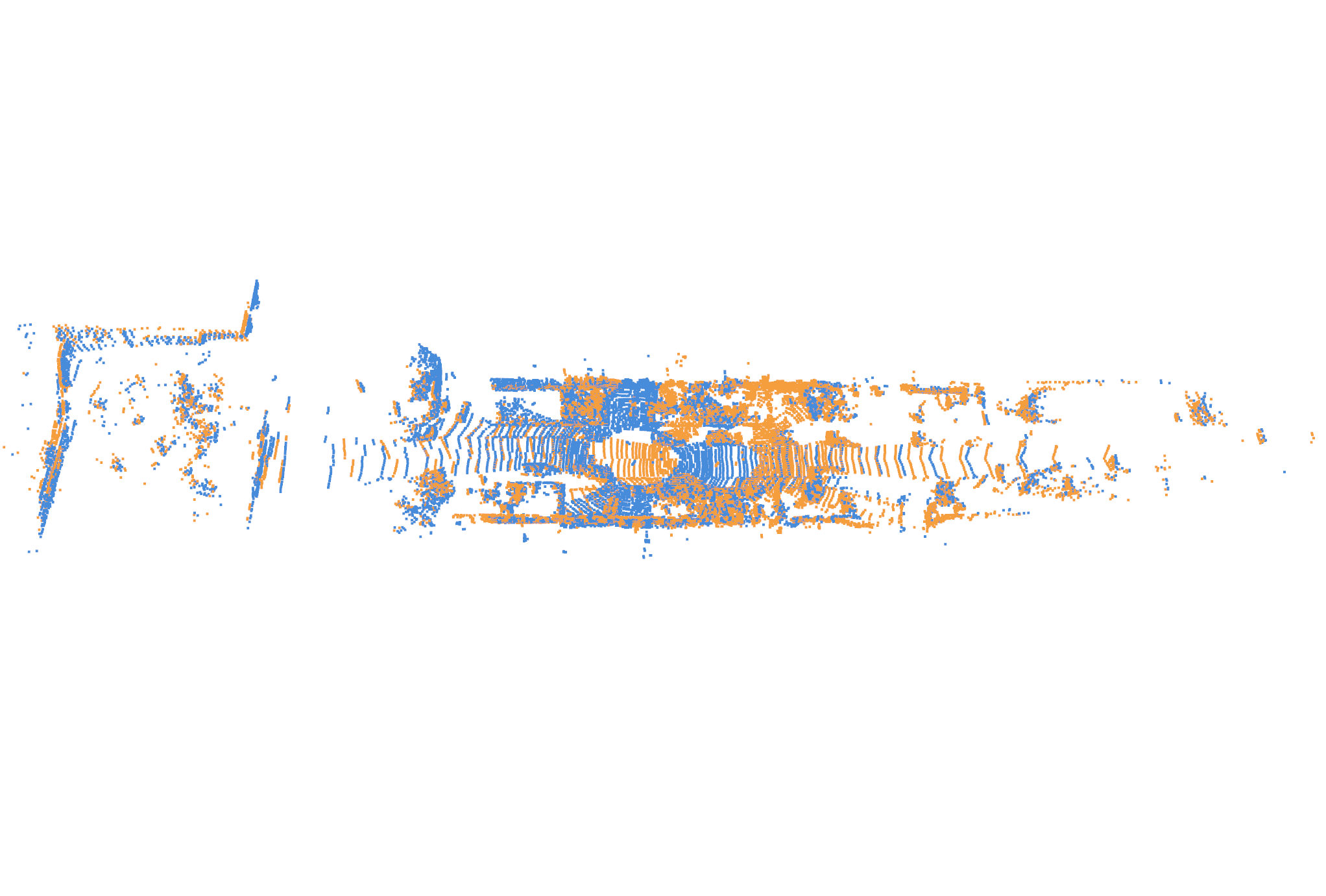
	(c-1) Initial ($73.73\%$ outlier)	(c-2) FGR[9]	(c-3) GC-RANSAC[14]	(c-4) Ours
	-	$E_{\bm{R}}=0.220\degree$	$E_{\bm{R}}=0.294\degree$	$E_{\bm{R}}=\textbf{0.212}\degree$
	-	$E_{\bm{t}}=0.521$\mathrm{m}$$	$E_{\bm{t}}=0.510$\mathrm{m}$$	$E_{\bm{t}}=\textbf{0.374}$\mathrm{m}$$
	-	${time}=1.258$s	${time}=1.576$s	${time}=\textbf{0.562}$s
Correspondence-free
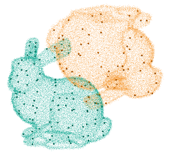
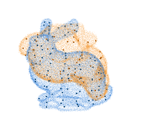
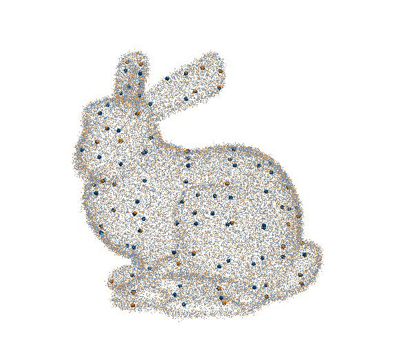
	(d-1) Initial ($60\%$ overlap)	(d-2) ICP[10]	(d-3) GoICP[11]	(d-4) Ours
	-	$E_{\bm{R}}=173.7\degree$	$E_{\bm{R}}=2.092\degree$	$E_{\bm{R}}=\textbf{0.061}\degree$
	-	$E_{\bm{t}}=0.240$\mathrm{m}$$	$E_{\bm{t}}=0.017$\mathrm{m}$$	$E_{\bm{t}}=\textbf{0.004}$\mathrm{m}$$
	-	${time}=\textbf{0.069}$s	${time}=80.40$s	${time}=2.524$s

Figure 1: The proposed method can efficiently address the rigid registration problem in different scenarios with high outlier rates or low overlap rates. For the correspondence-based registration problem, the input correspondences are generated by the traditional descriptor FPFH[15] and the learning-based descriptor FCGF[16]. The input point clouds are selected from (a) Bremen dataset[17], (b) ETH dataset[18], (c) KITTI dataset[19], and (d) Bunny dataset[20], respectively. The source point cloud is green, the target point cloud is yellow, and the aligned point cloud is blue. Compared with state-of-the-art correspondence-based methods, the proposed method achieves significant performance in terms of robustness and efficiency. Besides, the proposed method also can solve the SPCR problem efficiently and robustly.

Current 3D feature matching approaches have made satisfactory development. However, outlier correspondences are still inevitable either for handcrafted or learning-based descriptors[16, 21, 22]. Several paradigms have been extensively developed to implement robust registration, of which the consensus maximization is inherently robust to outliers without smoothing or trimming to change the objective function[23, 24]. Random sample consensus (RANSAC) is the most popular heuristic method for solving the consensus maximization problem of correspondence-based registration. However, RANSAC and its variants are non-deterministic and only generate satisfactory solutions with a certain probability due to the random sampling mechanism[25, 14].

More recently, many global and deterministic methods based on the branch and bound (BnB) framework have been applied to solve the point cloud registration problem with optimality guarantees[26, 11, 27, 28, 29, 13, 30, 31]. However, the computational complexity of BnB optimization is exponential to the dimension of the solution domain. Most studies address the issue by jointly searching for the optimal solution in $\mathbb{SE}(3)$[11, 27, 28]. In order to improve the algorithm efficiency, one direction is utilizing the known gravity directions measured by inertial measurement units (IMUs) to reduce the dimension of the parameter space to 4-dimensional[32, 33]. Another direction for reducing the problem dimension is to decompose the original problem into two 3-DOF sub-problems by leveraging the geometric properties[29, 13, 30, 12]. Typically, two unique features are employed for pose decoupling, i.e., the rotation invariant features (RIFs)[30, 34] and the translation invariant measurements (TIMs)[35, 12]. Nonetheless, the pairwise features make the number of input data increase squarely. Furthermore, a more efficient strategy is proposed based on the rotation decomposition, which decouples 6-DOF transformation into i) (2+1)-DOF, i.e., 2-DOF rotation axis and 1-DOF of translation along the axis, and ii) (1+2)-DOF, i.e., the remaining 1-DOF rotation and 2-DOF translation[31].

In contrast, we propose a novel efficient and deterministic search strategy based on residual projections for the rigid registration problem, in which a novel pose decoupling strategy is introduced. Specifically, we decouple the 6-DOF original problem into three 2-DOF rotation search sub-problems by projecting the residuals based on the Chebyshev distance, i.e., $L_{\infty}$ residual[36, 37], on the coordinate axes. We define the consensus maximization objective function for each sub-problem and apply a BnB-based optimization method to search for the solution globally and deterministically. We derive a novel polynomial-time upper bound for our objective function based on the interval stabbing technology[13, 32, 38]. The proposed method sequentially searches for three 2-DOF rotation matrix components by BnB. Meanwhile, the translation projections on the coordinate axes are implicitly estimated by interval stabbing. After solving these three sub-problems, we can finally obtain the optimal 6-DOF transformation. Compared with existing methods, the parameter space of the proposed method only is 2-dimensional, thus enhancing the computational efficiency, as shown in Fig. 1.

Notably, in contrast to existing BnB-based approaches, the proposed method requires no initialization of the translation domain, which is challenging to be accurately determined in different practical scenarios. Therefore, it avoids the problems that would arise when the translation domain is not initialized correctly. Notably, we can also partially verify if the total solution of the decomposed sub-problems is near the globally-optimal solution of the original problem by checking whether the solutions of the three sub-problems are orthogonal. Because the rotation matrix inherently is orthogonal.

The main contributions of this paper can be summarized as follows:

• We propose a novel pose decoupling strategy based on the $L_{\infty}$ residual projections. Compared with existing methods, our approach searches for the optimal solution in the low-dimensional solution domain, thereby improving search efficiency.

• We propose a novel BnB-based efficient and deterministic search method for each decoupled sub-problem. Specifically, we define the inlier set maximization objective function and derive the upper bound for our objective based on the interval stabbing technology.

• Due to its significant robustness, the proposed method can be extended to solve the challenging SPCR problem. We adapt the proposed upper bound to the extended objective function by interval merging technology.

The rest of this paper is organized as follows: The next section addresses the related work in two directions and discusses the innovations of the proposed method. Section 3 illustrates the problem formulation of our proposed method. Section 4 demonstrates the principle and details of our method. Section 5 presents extensive experimental results on both synthetic and real-world datasets. Finally, Section 6 gives a conclusion.

2 Related Work

As discussed in the previous section, there are two paradigms for the rigid point cloud registration problem regarding whether putative correspondences are given, i.e., correspondence-based registration and SPCR.

2.1 Correspondence-Based Registration

The correspondence-based registration comprises two steps: i) extract the 3D key-points and build putative correspondences by 3D feature descriptors, and ii) estimate the 6-DOF transformation based on the given correspondences. When the correspondences are correct, the registration problem has the elegant closed-form solution[39], although the non-convexity of $\mathbb{SO}(3)$. However, outliers in putative correspondences are inevitable in practical applications either for handcrafted or learning-based 3D descriptors[16, 15]. Therefore, robust registration techniques are indispensable. Consensus maximization is one of the most popular paradigms to address the robust registration problem, of which heuristic RANSAC[40] is the most representative. During each iteration, RANSAC employs a minimal solver to calculate the 3-DOF rotation and the 3-DOF translation separately. However, RANSAC only works efficiently under the conditions of low outlier rates. Recently, several RANSAC-based variants[41, 14, 42, 43] are proposed by introducing novel sampling strategies or local optimization methods. For instance, Graph-cut RANSAC[14] (GC-RANSAC) introduced the graph-cut algorithm to improve the local optimization performance. Nonetheless, RANSAC-based methods are non-deterministic and generate a correct solution only with a certain probability due to the essence of random sampling[25].

Given this context, numerous deterministic and robust correspondence-based registration methods have been proposed, most of which rely on the globally-optimal BnB framework[13, 32, 31, 33]. The fundamental concept underlying BnB involves the iterative alternation between solution domain segmentation (branch) and sub-branch bounds computation (bound) until the globally-optimal solution is obtained. Parra and Chin[13] proposed a guaranteed outlier removal (GORE) method, which leverages geometrical bounds to prune outliers and guarantees that eliminated correspondences are not the inlier. GORE converts the 6-DOF registration problem to a 3DOF rotational registration problem and then utilizes BnB to maximize the inlier set. Similar to GORE, Cai et al.[32] presented a deterministic pre-processing method to prune outliers for the 4-DOF terrestrial LiDAR registration problem. More recently, Chen et al.[31] introduced an efficient decomposition scheme for the 6-DOF rigid registration, which decouples the 6-DOF original problem into a (2+1)-DOF sub-problem and a (1+2)-DOF sub-problem. These two 3-DOF sub-problems are then sequentially solved by BnB-based search methods. On the other hand, a representative method of the deterministic M-estimation paradigm is FGR[9]. This method formulates the registration problem by the Geman-McClure objective function and then combines graduated non-convexity (GNC) to solve the problem. Although the high efficiency of this method, it is easy to generate incorrect solutions at a high outlier rate. Combining the ideas of outlier removal and M-estimation, Yang et al.[12] proposed a certifiable and deterministic approach, i.e., Truncated least squares Estimation And SEmidefinite Relaxation (TEASER). TEASER leverages TIMs to decouple the 6-DOF transformation search problem into a 3-DOF rotation search sub-problem followed by a 3-DOF translation search sub-problem. Meanwhile, TEASER allows outlier pruning by maximum clique method [44], which, however requires quadratic memory space ($\mathcal{O}(N^{2})$). As mentioned before, existing decoupling-based methods typically decompose the original 6-DOF problem into two 3-DOF sub-problems. Motivated by this observation, our study aims to develop a novel pose decoupling strategy to search the optimal parameters in low-dimensional space by exploring the geometric properties of the rigid point cloud registration problem.

2.2 Simultaneous Pose and Correspondence Registration

The SPCR problem is more challenging since the transformation and correspondences need to be estimated simultaneously. A typical algorithm is ICP[10], an expectation-maximization (EM) type method. However, ICP is susceptible to local minima and is greatly influenced by the initialization of the transformation. Another series of noise-robust methods represent the point cloud as Gaussian mixture models (GMMs) to build robust objective functions based on the probability density[45, 46]. Although all these methods can efficiently converge to an optimum when they are initialized well, they can not provide any optimality guarantees.

Another line for the SPCR problem is to estimate the globally-optimal solution without initialization, which is commonly based on the BnB framework[11, 28, 27, 29, 30]. Go-ICP[11] is the first practical globally-optimal approach for the 6-DOF SPCR problem that employs the nested BnB search structure to minimize the objective function based on the $L_{2}$ residual. Parra et al.[28] formulated the registration as a consensus maximization problem and proposed a BnB-based method with a tighter bound than Go-ICP. Campbell et al.[27] proposed a more efficient and robust BnB-based approach to minimize the GMM-based objective function. However, both these methods jointly search for the globally-optimal solution over the 6-dimensional parameter space, leading to relatively high computational costs. One common direction to improve efficiency is reducing the dimension of the solution domain by decoupling the transformation. For instance, Straub et al.[29] proposed a decoupling method based on surface normal distributions that decomposes the 6-DOF registration problem into the separate 3-DOF rotation and 3-DOF translation sub-problems. Liu et al.[30] introduced the RIFs to enable sequential estimations of the 3-DOF translation and the 3-DOF rotation instead of the joint 6-DOF transformation estimation. By contrast, the proposed method not only has a novel decoupling strategy based on residual projections, but also can be extended to solve the SPCR problem by adjusting the objective and bound functions. The detailed formulation will be given in Section 4.3.

3 Problem Formulation

3.1 Inlier Set Maximization

Given the source point cloud $\mathcal{P}$ and the target point cloud $\mathcal{Q}$, a set of putative correspondences $\mathcal{K}=\left\{(\bm{p}_{i},\bm{q}_{i})\right\}_{i=1}^{N}$ is extracted by matching points between $\mathcal{P}$ and $\mathcal{Q}$, where $\bm{p}_{i},\bm{q}_{i}\in\mathbb{R}^{3}$, and $N$ is the correspondences number. The proposed method aims to estimate the rigid transformation between the source and target point clouds. Specifically, the 6-DOF transformation matrix $\bm{T}\in\mathbb{SE}(3)$ is formed by the 3-DOF rotation matrix $\bm{R}\in\mathbb{SO}(3)$ and the 3-DOF translation vector $\bm{t}\in\mathbb{R}^{3}$. The rotation matrix $\bm{R}$ is an orthogonal matrix in which the columns and rows are orthogonal vectors, i.e., $\bm{R}\bm{R}^{\mathrm{T}}=\bm{I}$. Formally, we adopt the inlier set maximization formulation for the robust registration problem:

$$\bm{T}^{*}=\mathop{\arg\max}_{\bm{T}\in\mathbb{SE}(3)}\mathcal{C}\left(\bm{T}(\mathcal{P}),\mathcal{Q}\right),$$ (1)

where $\mathcal{C}$ is the objective function for calculating the cardinality of the inlier set.

Different from existing approaches[11, 28, 13, 32, 31] that commonly employ the $L_{2}$ residual to measure the alignment, we apply the Chebyshev distance, i.e., $L_{\infty}$ residual[36, 37, 30], to build the robust objective function. Therefore, considering the presence of noise, we estimate the rotation and translation that maximize the objective:

$$E(\bm{R},\bm{t}|\mathcal{K},\epsilon)=\sum_{i=1}^{N}\mathbb{I}\left(\left\|\bm{R}\bm{p}_{i}+\bm{t}-\bm{q}_{i}\right\|_{\infty}\leq\epsilon\right),$$ (2)

where $\mathbb{I}(\cdot)$ is the indicator function that returns 1 if the input condition is true and 0 otherwise, $\left\|\cdot\right\|_{\infty}$ denotes the $L_{\infty}$-norm, and $\epsilon$ is the inlier threshold.

3.2 Residual Projections and Pose Decoupling

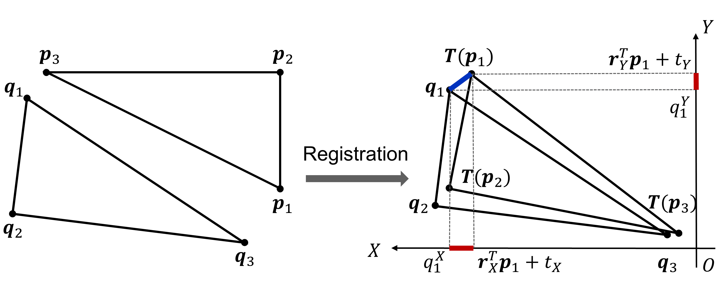
Figure 2: A toy 2D registration example to demonstrate $L_{\infty}$ residual projection. Specifically, $\left\{(\bm{p}_{i},\bm{q}_{i})\right\}_{i=1}^{3}$ is the set of input correspondences, the red line segments represent the projections of the residual on the coordinate axes $X$ and $Y$, i.e., $\left|\bm{r}_{j}^{\mathrm{T}}\bm{p}_{1}+t_{j}-q_{1}^{j}\right|$, $j=X,Y$. The inlier constraint for $L_{\infty}$ residual indicates that, $(\bm{p}_{1},\bm{q}_{1})$ is an inlier only if both residual projections on the coordinate axes are not larger than the inlier threshold.

Mathematically, we apply the following definitions to derive the residual projections. Firstly, we denote the rotation matrix as

$$\bm{R}\triangleq\begin{bmatrix}r_{X1}&r_{X2}&r_{X3}\\ r_{Y1}&r_{Y2}&r_{Y3}\\ r_{Z1}&r_{Z2}&r_{Z3}\end{bmatrix}=\begin{bmatrix}\bm{r}_{X}&\bm{r}_{Y}&\bm{r}_{Z}\end{bmatrix}^{\mathrm{T}}.$$ (3)

where $\bm{r}_{j}=\left[r_{j1},r_{j2},r_{j3}\right]^{\mathrm{T}}$, $j=X,Y,Z$, is the transpose of each row of the rotation matrix. The translation vector is

$$\bm{t}\triangleq\left[t_{X},t_{Y},t_{Z}\right]^{\mathrm{T}}.$$ (4)

Given the definitions of $\bm{R}$ and $\bm{t}$, according to the definition of Chebyshev distance, the inlier constraint in the objective function (2) can be rewritten as

$$\left\|\bm{R}\bm{p}_{i}+\bm{t}-\bm{q}_{i}\right\|_{\infty}\leq\epsilon$$ (5a)

$$\Leftrightarrow \left\|\begin{bmatrix}\bm{r}_{X}^{\mathrm{T}}\\ \bm{r}_{Y}^{\mathrm{T}}\\ \bm{r}_{Z}^{\mathrm{T}}\end{bmatrix}\bm{p}_{i}+\begin{bmatrix}t_{X}\\ t_{Y}\\ t_{Z}\end{bmatrix}-\begin{bmatrix}{q}_{i}^{X}\\ {q}_{i}^{Y}\\ {q}_{i}^{Z}\\ \end{bmatrix}\right\|_{\infty}\leq\epsilon$$ (5b)

$$\Leftrightarrow \mathop{\max}\left\{\begin{aligned} &\left|\bm{r}_{X}^{\mathrm{T}}\bm{p}_{i}+t_{X}-q_{i}^{X}\right|,\\ &\left|\bm{r}_{Y}^{\mathrm{T}}\bm{p}_{i}+t_{Y}-q_{i}^{Y}\right|,\\ &\left|\bm{r}_{Z}^{\mathrm{T}}\bm{p}_{i}+t_{Z}-q_{i}^{Z}\right|\end{aligned}\right\}\leq\epsilon$$ (5c)

$$\Leftrightarrow \left\{\begin{aligned} &\left|\bm{r}_{X}^{\mathrm{T}}\bm{p}_{i}+t_{X}-q_{i}^{X}\right|\leq\epsilon,\\ &\left|\bm{r}_{Y}^{\mathrm{T}}\bm{p}_{i}+t_{Y}-q_{i}^{Y}\right|\leq\epsilon,\\ &\left|\bm{r}_{Z}^{\mathrm{T}}\bm{p}_{i}+t_{Z}-q_{i}^{Z}\right|\leq\epsilon\end{aligned}\right.$$ (5d)

$$\Leftrightarrow \left\{\begin{aligned} &\mathbb{I}\left(\left|\bm{r}_{X}^{\mathrm{T}}\bm{p}_{i}+t_{X}-q_{i}^{X}\right|\leq\epsilon\right)=1,\\ &\mathbb{I}\left(\left|\bm{r}_{Y}^{\mathrm{T}}\bm{p}_{i}+t_{Y}-q_{i}^{Y}\right|\leq\epsilon\right)=1,\\ &\mathbb{I}\left(\left|\bm{r}_{Z}^{\mathrm{T}}\bm{p}_{i}+t_{Z}-q_{i}^{Z}\right|\leq\epsilon\right)=1\end{aligned}\right.$$ (5e)

where $\bm{q}_{i}\triangleq\left[q_{i}^{X},q_{i}^{Y},q_{i}^{Z}\right]^{\mathrm{T}}$, and $\left|\bm{r}_{j}^{\mathrm{T}}\bm{p}_{i}+t_{j}-q_{i}^{j}\right|$, $j=X,Y,Z$, are projections of the $i$-th residual on the coordinate axes, as shown in Fig. 2. Then we can set $\mathbb{I}\left(\left|\bm{r}_{j}^{\mathrm{T}}\bm{p}_{i}+t_{j}-q_{i}^{j}\right|\leq\epsilon\right)=\mathcal{L}_{i}^{j}$. Therefore, the objective function (2) can be reformulated as

$$E(\bm{R},\bm{t}|\mathcal{K},\epsilon)=\sum_{i=1}^{N}\mathbb{I}\left(\mathcal{L}_{i}^{X}\land\mathcal{L}_{i}^{Y}\land\mathcal{L}_{i}^{Z}\right),$$ (6)

where $\land$ is the logical AND operation.

Geometrically, the objective function (6) indicates that, given an arbitrary correspondence $(\bm{p}_{i},\bm{q}_{i})$ and the inlier threshold $\epsilon$, only when the residual projections on the $X$, $Y$, and $Z$ coordinate axes are not larger than $\epsilon$, $(\bm{p}_{i},\bm{q}_{i})$ is an inlier, as shown in Fig. 2. Notably, these three conditions are equally independent. Accordingly, we may reduce the original constraint in Eq. (6) as three separate constraints, i.e., $\mathcal{L}_{i}^{X}$, $\mathcal{L}_{i}^{Y}$, and $\mathcal{L}_{i}^{Z}$.

In this way, the original search problem for the transformation in $\mathbb{SE}(3)$ can be decoupled into three sub-problems. The new inlier set maximization objective for each sub-problem can be

$$E_{j}(\bm{r}_{j},t_{j}|\mathcal{K},\epsilon)=\sum_{i=1}^{N}\mathbb{I}\left(\left|\bm{r}_{j}^{\mathrm{T}}\bm{p}_{i}+t_{j}-q_{i}^{j}\right|\leq\epsilon\right),j=X,Y,Z.$$ (7)

In other words, we reformulate the $L_{\infty}$ residual-based objective function in the form of residual projections. Then we decompose the joint constraint into three independent constraints to decouple the original registration problem into three sub-problems, i.e., $\max E_{X}(\bm{r}_{X},t_{X}|\mathcal{K},\epsilon)$, $\max E_{Y}(\bm{r}_{Y},t_{Y}|\mathcal{K},\epsilon)$, and $\max E_{Z}(\bm{r}_{Z},t_{Z}|\mathcal{K},\epsilon)$. In the next section, we will introduce a step-wise search strategy to solve these three sub-problems.

4 Step-wise Search Strategy Based on Branch and Bound

Branch and bound (BnB) is an algorithm framework for global optimization. To design the BnB-based algorithm, two main aspects need to be addressed, i) how to parameterize and branch the solution domain, and ii) how to efficiently calculate the upper and lower bounds. Then the BnB-based algorithm can recursively divide the solution domain into smaller spaces and prune the sub-branches by upper and lower bounds until convergence.

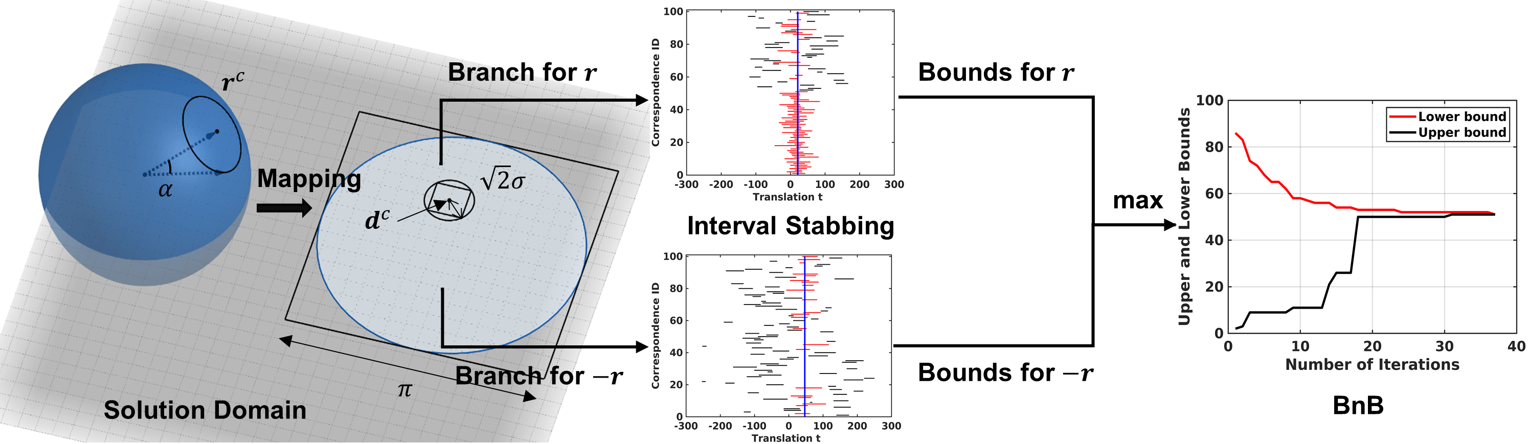
Figure 3: The solution domain before and after exponential mapping, and the pipeline of our proposed BnB algorithm. The original solution domain of the vector $\bm{r}$ is a unit sphere in the 3D Euclidean space. The exponential mapping method maps the unit sphere to two identical 2D disks, representing the solution domains of $\bm{r}$ and $-\bm{r}$, respectively. We can only branch one 2D-disk domain during each iteration, followed by the calculation of upper and lower bounds for each sub-branch. The proposed BnB algorithm converges until the optimal solution $\bm{r}^{*}$ is found, and the optimal $t^{*}$ is found by interval stabbing at the same time. In the visualization results of interval stabbing, the black line segments are the candidate intervals of each correspondence, and the red line segments are the intervals crossed by the blue probe with the max-stabbing number. The probe position is the max-stabbing position.

4.1 Parametrization of Solution Domain

4.1.1 Rotation

For each sub-problem of the objective function (7), the unknown-but-sought vector $\bm{r}_{j}$ (denoted by $\bm{r}$ in this section) is in a unit sphere (denoted by $\mathbb{S}^{2}$). Then we divide the unit sphere into two unit hemispheres ($\mathbb{S}^{2+}$ and $\mathbb{S}^{2-}$) to represent the parameter spaces of the “positive” vector $\bm{r}$ and the “negative” vector $-\bm{r}$. The “upper” hemisphere is defined as

$$\mathbb{S}^{2+}=\left\{\bm{r}|\bm{r}^{\mathrm{T}}\bm{r}=1,r_{3}\geq 0\right\},$$ (8)

where $\bm{r}\triangleq[r_{1},r_{2},r_{3}]^{\mathrm{T}}$ is a unit vector in $\mathbb{R}^{3}$. Geometrically, since these two hemispheres are centrally symmetric, the “lower” hemisphere is $\mathbb{S}^{2-}$ which can be seen as $-\mathbb{S}^{2+}$. In order to parametrize $\mathbb{S}^{2+}$ and $\mathbb{S}^{2-}$ minimally, we introduce the exponential mapping[47, 48] technology to map a 3-dimensional hemisphere to a 2-dimensional disk efficiently. Specifically, given a vector $\bm{r}\in\mathbb{S}^{2+}$, it can be represented by a corresponding point $\bm{d}\in\mathbb{R}^{2}$ in the 2D disk, i.e.,

$$\bm{r}^{\mathrm{T}}=\left[\sin(\gamma)\hat{\bm{d}}^{\mathrm{T}},\cos(\gamma)\right],\quad\text{and}\quad\bm{d}=\gamma\hat{\bm{d}}$$ (9)

where $\gamma\in[0,\pi/2]$, $\hat{\bm{d}}^{\mathrm{T}}=\bm{d}/\|\bm{d}\|$ is a unit vector in $\mathbb{R}^{2}$. Notably, the range of $\gamma$ corresponds to $r_{3}\geq 0$, and its maximum corresponds to the radius of the 2D disk, i.e., $\pi/2$, as shown in Fig. 3. For a vector $-\bm{r}\in\mathbb{S}^{2-}$, we define another exponential mapping method,

$$-\bm{r}^{\mathrm{T}}=-\left[\sin(\gamma)\hat{\bm{d}}^{\mathrm{T}},\cos(\gamma)\right].$$ (10)

Accordingly, the total solution domain (unit sphere) is mapped as two identical 2D disks, which represent the parameter spaces of $\bm{r}$ and $-\bm{r}$, respectively. Compared to the unit sphere representation within three parameters and a unit-norm constraint, the exponential mapping is a more compact representation within only two parameters[48]. Meanwhile, for ease of operation, a circumscribed square of the disk domain is initialized as the domain of $\bm{r}$ in the proposed BnB algorithm, and the domain of $-\bm{r}$ is relaxed in the same way.

Further, we introduce the following lemma[47] about the exponential mapping between $\mathbb{S}^{2+}$ and $\mathbb{R}^{2}$.

Lemma 1.

$\bm{r}_{a},\bm{r}_{b}\in\mathbb{S}^{2+}$ are two vectors in the unit hemisphere, and $\bm{d}_{a},\bm{d}_{b}\in\mathbb{R}^{2}$ are corresponding points in the 2D disk. Then we have

$$\angle(\bm{r}_{a},\bm{r}_{b})\leq\left\|\bm{d}_{a}-\bm{d}_{b}\right\|.$$ (11)

According to Lemma 1, we can obtain the following proposition.

Proposition 1.

Given a sub-branch of the square-shaped domain $\mathbb{D}$, its center is $\bm{d}^{c}\in\mathbb{R}^{2}$ and half-side length is $\sigma$. For $\forall\bm{d}\in\mathbb{D}$, we have

$$\angle\left(\bm{r},\bm{r}^{c}\right)\leq\left\|\bm{d}-\bm{d}^{c}\right\|\leq\sqrt{2}\sigma,$$ (12)

where $\bm{r}$ and $\bm{r}^{c}$ correspond to $\bm{d}$ and $\bm{d}^{c}$, respectively.

Defining $\alpha\triangleq\max\angle\left(\bm{r},\bm{r}^{c}\right)$, we can obtain $\alpha\leq\sqrt{2}\sigma$ with Proposition 1, as shown in Fig. 3. Geometrically, Proposition 1 indicates that one square-shaped sub-branch of the 2D disk domain is relaxed to a spherical patch of the 3D unit sphere. In addition, Lemma 1 and Proposition 1 hold for both hemispheres $\mathbb{S}^{2+}$ and $\mathbb{S}^{2-}$. In this study, we apply Proposition 1 as one of the fundamental parts to derive our proposed bounds.

4.1.2 Translation

Estimating the translation component $t_{j}\in\mathbb{R}$, $j=X,Y,Z$ in the objective function (7) is a 1-dimensional problem. The translation is unconstrained, and it is not easy to estimate a suitable solution domain accurately in advance for various practical scenarios. Existing BnB-based approaches[11, 31, 30] commonly initialize the translation domain as a redundant space and search it exhaustively, leading to a significant decrease in efficiency. Meanwhile, if the translation domain is not initialized correctly, the algorithm may not find the optimal (correct) solution since the optimal solution may be excluded from the initial search domain.

In our study, we propose an interval stabbing-based method to estimate the translation components $\{t_{X},t_{Y},t_{Z}\}$ without any prior information on the size of the translation domain, which can effectively reduce the total parameter space and improve the algorithm efficiency. It also avoids the problems that may arise when the translation initialization is incorrect. The proposed method will be described thoroughly in Section 4.2.

4.2 Interval Stabbing and Bounds

We first introduce the following lemma to derive the bounds for the objective function (7).

Lemma 2.

Given an arbitrary consensus maximization objective $F(x|A)=\sum_{i=1}^{M}\mathcal{F}_{i}\left(x,a_{i}\right)$, where $x$ is the variable to be calculated, $A=\left\{a_{i}\right\}_{i=1}^{M}$ is the set of input measurements, and $\mathcal{F}_{i}(x,a_{i})$ is an indicator function with a certain constraint. Then we have

$$\mathop{\max}_{x}F(x|A)=\mathop{\max}_{x}\sum_{i=1}^{M}\mathcal{F}_{i}\left(x,a_{i}\right)\leq\sum_{i=1}^{M}\mathop{\max}_{x}\mathcal{F}_{i}\left(x,a_{i}\right).$$ (13)

Proof.

For the $i$-th input measurement $a_{i}$, we can obtain $\mathcal{F}_{i}\left(x,a_{i}\right)\leq\mathop{\max}_{x}\mathcal{F}_{i}\left(x,a_{i}\right)\leq 1$. Therefore, it is obvious that the maximum of $\sum_{i=1}^{M}\mathcal{F}_{i}\left(x,a_{i}\right)$ is not bigger than the sum of $\mathop{\max}_{x}\mathcal{F}_{i}\left(x,a_{i}\right)$. ∎

In this study, the upper and lower bounds are proposed as follows:

Proposition 2 (Upper bound for $\mathbb{S}^{2+}$).

Given a sub-branch of the square-shaped domain $\mathbb{D}$, whose center is $\bm{d}^{c}\in\mathbb{R}^{2}$ (corresponds to $\bm{r}_{j}^{c}\in\mathbb{S}^{2+}$) and half-side length is $\sigma$, the upper bound can be set as

$$\overline{E}^{+}(\mathbb{D})=\mathop{\max}_{t_{j}}\sum_{i=1}^{N}\mathbb{I}\left(t_{j}\in\left[t_{j}^{i-},t_{j}^{i+}\right]\right),$$ (14a)

$$t_{j}^{i-}=-\epsilon-\left\|\bm{p}_{i}\right\|\cos\left(\mathop{\max}\left\{\angle\left(\bm{r}_{j}^{c},\bm{p}_{i}\right)-\sqrt{2}\sigma,0\right\}\right)+q_{i}^{j},$$ (14b)

$$t_{j}^{i+}=\epsilon-\left\|\bm{p}_{i}\right\|\cos\left(\mathop{\min}\left\{\angle\left(\bm{r}_{j}^{c},\bm{p}_{i}\right)+\sqrt{2}\sigma,\pi\right\}\right)+q_{i}^{j}.$$ (14c)

Proof.

First, we rewrite the maximum of the objective function (7) as,

$$\mathop{\max}_{\bm{r}_{j},t_{j}}\sum_{i=1}^{N}\mathcal{L}_{i}^{j}=\mathop{\max}_{t_{j}}\mathop{\max}_{\bm{r}_{j}}\sum_{i=1}^{N}\mathcal{L}_{i}^{j}.$$ (15)

Therefore, according to Lemma 2, we have

$$\mathop{\max}_{t_{j}}\mathop{\max}_{\bm{r}_{j}}\sum_{i=1}^{N}\mathcal{L}_{i}^{j}\leq\mathop{\max}_{t_{j}}\sum_{i=1}^{N}\mathop{\max}_{\bm{r}_{j}}\mathbb{I}\left(\left|\bm{r}_{j}^{\mathrm{T}}\bm{p}_{i}+t_{j}-q_{i}^{j}\right|\leq\epsilon\right).$$ (16)

Additionally, given a sub-branch $\mathbb{D}$, according to the triangle inequality in spherical geometry[24] and Proposition 1, we have

$$\angle\left(\bm{r}_{j},\bm{p}_{i}\right) \leq\angle\left(\bm{r}_{j}^{c},\bm{p}_{i}\right)+\angle\left(\bm{r}_{j}^{c},\bm{r}_{j}\right)$$ (17a)

$$\leq\angle\left(\bm{r}_{j}^{c},\bm{p}_{i}\right)+\alpha$$ (17b)

$$\leq\angle\left(\bm{r}_{j}^{c},\bm{p}_{i}\right)+\sqrt{2}\sigma,$$ (17c)

and

$$\angle\left(\bm{r}_{j},\bm{p}_{i}\right) \geq\angle\left(\bm{r}_{j}^{c},\bm{p}_{i}\right)-\angle\left(\bm{r}_{j}^{c},\bm{r}_{j}\right)$$ (18a)

$$\geq\angle\left(\bm{r}_{j}^{c},\bm{p}_{i}\right)-\alpha$$ (18b)

$$\geq\angle\left(\bm{r}_{j}^{c},\bm{p}_{i}\right)-\sqrt{2}\sigma.$$ (18c)

Thus, according to $\bm{r}_{j}^{\mathrm{T}}\bm{p}_{i}=\left\|\bm{r}_{j}\right\|\left\|\bm{p}_{i}\right\|\cos\angle\left(\bm{r}_{j},\bm{p}_{i}\right)$ and $\left\|\bm{r}_{j}\right\|=1$, we have

$$\bm{r}_{j}^{\mathrm{T}}\bm{p}_{i}\in\Big{[} \left\|\bm{p}_{i}\right\|\cos\left(\mathop{\min}\left\{\angle\left(\bm{r}_{j}^{c},\bm{p}_{i}\right)+\sqrt{2}\sigma,\pi\right\}\right),$$ (19)

$$\left\|\bm{p}_{i}\right\|\cos\left(\mathop{\max}\left\{\angle\left(\bm{r}_{j}^{c},\bm{p}_{i}\right)-\sqrt{2}\sigma,0\right\}\right)\Big{]}.$$

Then, given a sub-branch $\mathbb{D}$, whose center is $\bm{d}^{c}$ (corresponds to $\bm{r}_{j}^{c}$) and half-side length is $\sigma$, we can observe that,

$$\mathop{\max}_{\bm{r}_{j}}\mathbb{I}\left(\left|\bm{r}_{j}^{\mathrm{T}}\bm{p}_{i}+t_{j}-q_{i}^{j}\right|\leq\epsilon\right)$$ (20a)

$$= \mathop{\max}_{\bm{r}_{j}}\mathbb{I}\left(-\epsilon-\bm{r}_{j}^{\mathrm{T}}\bm{p}_{i}+q_{i}^{j}\leq t_{j}\leq\epsilon-\bm{r}_{j}^{\mathrm{T}}\bm{p}_{i}+q_{i}^{j}\right)$$ (20b)

$$\leq \mathbb{I}\left(t_{j}\in\left[t_{j}^{i-},t_{j}^{i+}\right]\right),$$ (20c)

where

$$t_{j}^{i-} =-\epsilon-\left\|\bm{p}_{i}\right\|\cos\left(\mathop{\max}\left\{\angle\left(\bm{r}_{j}^{c},\bm{p}_{i}\right)-\sqrt{2}\sigma,0\right\}\right)+q_{i}^{j},$$ (21a)

$$t_{j}^{i+} =\epsilon-\left\|\bm{p}_{i}\right\|\cos\left(\mathop{\min}\left\{\angle\left(\bm{r}_{j}^{c},\bm{p}_{i}\right)+\sqrt{2}\sigma,\pi\right\}\right)+q_{i}^{j}.$$ (21b)

Then,

$$\sum_{i=1}^{N}\mathop{\max}_{\bm{r}_{j}}\mathbb{I}\left(\left|\bm{r}_{j}^{\mathrm{T}}\bm{p}_{i}+t_{j}-q_{i}^{j}\right|\leq\epsilon\right)\leq\sum_{i=1}^{N}\mathbb{I}\left(t_{j}\in\left[t_{j}^{i-},t_{j}^{i+}\right]\right)$$ (22)

Finally, we have

$$\mathop{\max}_{\bm{r}_{j},t_{j}}\sum_{i=1}^{N}\mathcal{L}_{i}^{j}\leq\mathop{\max}_{t_{j}}\sum_{i=1}^{N}\mathbb{I}\left(t_{j}\in\left[t_{j}^{i-},t_{j}^{i+}\right]\right)$$ (23)

Therefore, Proposition 2 is proved. ∎

Proposition 3 (Upper bound for $\mathbb{S}^{2-}$).

Given a sub-branch of the square-shaped domain $\mathbb{D}$, whose center is $\bm{d}^{c}\in\mathbb{R}^{2}$ (corresponds to $-\bm{r}_{j}^{c}\in\mathbb{S}^{2-}$) and half-side length is $\sigma$, the upper bound can be set as

$$\overline{E}^{-}(\mathbb{D})=\mathop{\max}_{t_{j}}\sum_{i=1}^{N}\mathbb{I}\left(t_{j}\in\left[t_{j}^{i-},t_{j}^{i+}\right]\right),$$ (24a)

$$t_{j}^{i-}=-\epsilon+\left\|\bm{p}_{i}\right\|\cos\left(\mathop{\min}\left\{\angle\left(\bm{r}_{j}^{c},\bm{p}_{i}\right)+\sqrt{2}\sigma,\pi\right\}\right)+q_{i}^{j},$$ (24b)

$$t_{j}^{i+}=\epsilon+\left\|\bm{p}_{i}\right\|\cos\left(\mathop{\max}\left\{\angle\left(\bm{r}_{j}^{c},\bm{p}_{i}\right)-\sqrt{2}\sigma,0\right\}\right)+q_{i}^{j}.$$ (24c)

Proof.

The proof is similar to Proposition 2, which is simple enough that we omit it. ∎

Although the upper bounds in Proposition 2 and Proposition 3 are theoretically provided, we still need to find an appropriate method to compute them. Mathematically, the calculation of the upper bounds is a typical interval stabbing problem[49]. As shown in Fig. 3, the interval stabbing problem aims to find a probe (i.e., the blue line segment) that stabs the maximum number of intervals. There has been a deterministic and polynomial-time algorithm[32] to solve the interval stabbing problem. More details are given in [49, 32].

By utilizing the interval stabbing technology to compute the upper bounds, the proposed BnB-based method only needs to search a 2-dimensional solution domain, thereby improving the algorithm efficiency. Meanwhile, the translation projections $\{t_{X},t_{Y},t_{Z}\}$ are implicitly estimated by interval stabbing without requiring the initialization of the translation domain. In other words, the interval stabbing approach returns not only the max-stabbing number (i.e., the upper bound), but also the max-stabbing position (i.e., the estimation of $t_{j}$).

To sum up, considering the total solution domain $\mathbb{S}^{2+}$ and $\mathbb{S}^{2-}$, we have the following proposition.

Proposition 4 (Upper bound for $\mathbb{S}^{2}$).

Given a sub-branch of the square-shaped domain $\mathbb{D}$, whose center is $\bm{d}^{c}\in\mathbb{R}^{2}$ and half-side length is $\sigma$, the upper bound of the objective function (7), can be set as

$$\overline{E}(\mathbb{D})=\mathop{\max}\left\{\overline{E}^{+}(\mathbb{D}),\overline{E}^{-}(\mathbb{D})\right\}.$$ (25)

Proof.

The maximum of these two upper bounds is not smaller than the maximum of the objective function (7). Therefore, $\overline{E}(\mathbb{D})$ is the final upper bound of the objective function (7). ∎

Proposition 5 (Lower bound for $\mathbb{S}^{2}$).

Given a sub-branch of the square-shaped domain $\mathbb{D}$, whose center is $\bm{d}^{c}\in\mathbb{R}^{2}$ and half-side length is $\sigma$, the lower bound of the objective function (7) can be set as

$$\underline{E}(\mathbb{D})=\mathop{\max}\left\{\underline{E}^{+}(\mathbb{D}),\underline{E}^{-}(\mathbb{D})\right\},$$ (26a)

$$\underline{E}^{+}(\mathbb{D})=\sum_{i=1}^{N}\mathbb{I}\left(\left|\left(\bm{r}_{j}^{c}\right)^{\mathrm{T}}\bm{p}_{i}+\overline{t}_{j}^{+}-q_{i}^{j}\right|\leq\epsilon\right),$$ (26b)

$$\underline{E}^{-}(\mathbb{D})=\sum_{i=1}^{N}\mathbb{I}\left(\left|-\left(\bm{r}_{j}^{c}\right)^{\mathrm{T}}\bm{p}_{i}+\overline{t}_{j}^{-}-q_{i}^{j}\right|\leq\epsilon\right),$$ (26c)

where $\overline{t}_{j}^{+}$ is the max-stabbing position of the upper bound for $\mathbb{S}^{2+}$, and $\overline{t}_{j}^{-}$ is the max-stabbing position of the upper bound for $\mathbb{S}^{2-}$.

Proof.

The maximum of the objective function in the given sub-branch $\mathbb{D}$ should be no less than any objective value at a specific point. Therefore, $\underline{E}(\mathbb{D})$ is the lower bound of the objective function (7). ∎

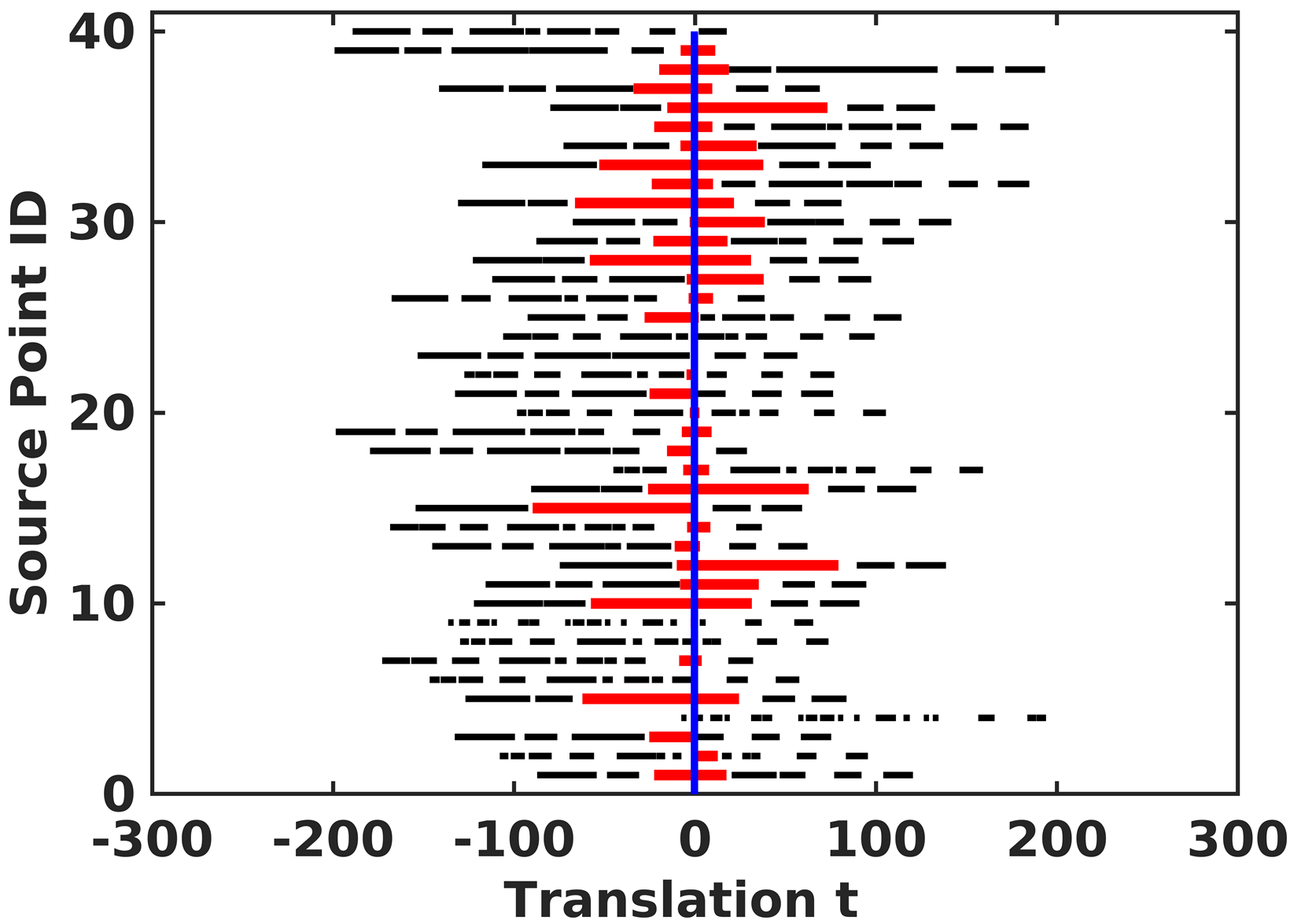
(a) SPCR Upper for $\mathbb{S}^{2+}$: 33	(b) SPCR Upper for $\mathbb{S}^{2-}$: 38

Figure 4: The visualization results for the 24-th iteration of a representative SPCR test on synthetic data. The final SPCR upper bound for $\mathbb{S}^{2}$ is 38. The black line segments are the intervals after interval merging, and the red line segments are the intervals crossed by the blue probe with the max-stabbing number.

Based on the upper and lower bounds in Proposition 4 and Proposition 5, the proposed BnB-based algorithm for the 2-DOF rotation matrix components search sub-problem is outlined in Algorithm 1. We employ the depth-first search strategy[50] to implement the proposed BnB algorithm. As we indicated in Section 4.1, although the initial solution domain $\mathbb{S}^{2}$ is mapped to two identical 2D-disks, only one disk domain is branched, since the bounds of $\mathbb{S}^{2+}$ and $\mathbb{S}^{2-}$ can be computed separately in the same disk domain, as shown in Fig. 3. During each iteration, the branch with maximal upper bound is partitioned into four sub-branches since the current parameter space is only 2-dimensional. Then the branch list is updated, and the upper and lower bounds for each sub-branch are estimated. The sub-branches that do not have a better solution than the best-so-far solution are eliminated. As the number of iterations increases, the gap between the upper and lower bounds gradually decreases. Until the gap reduces to zero, the BnB algorithm obtains the optimal solutions $\bm{r}_{j}^{*}$ and $t_{j}^{*}$. As shown in [30, 31], existing methods usually solve sub-problems sequentially. However, we can solve three sub-problems in an arbitrary order with Algorithm 1 and obtain the final optimal solution $\bm{R}^{*}$ and $\bm{t}^{*}$.

Input: The set of correspondences $\mathcal{K}=\left\{(\bm{p}_{i},\bm{q}_{i})\right\}_{i=1}^{N}$, inlier threshold $\epsilon$.

Output: Optimal solution $\bm{r}_{j}^{*}\in\mathbb{S}^{2}$ and $t_{j}^{*}\in\mathbb{R}$.

1Initialize the solution domain $\mathbb{D}_{0}$;

2 Initialize the list of sub-branches $\xi=\{\mathbb{D}_{0}\}$;

3 Initialize the lower bound $L=0$, and the upper bound $U=N$;

4 Define function $\delta(\mathbb{D})$ returns the center of sub-branch $\mathbb{D}$ corresponding to the upper bound;

5 Define function $\eta(\mathbb{D})$ returns the max-stabbing position of sub-branch $\mathbb{D}$ corresponding to the upper bound;

6 while $U-L>0$ do

7       Select a sub-branch $\mathbb{D}$ with the maximal upper bound from $\xi$, i.e., $\mathbb{D}=\mathop{\arg\max}\overline{E}(\mathbb{D}_{k})$, $\mathbb{D}_{k}\in\xi$;

8       Subdivide $\mathbb{D}$ into four sub-branches $\{\mathbb{D}_{1},\dots,\mathbb{D}_{4}\}$;

9       Insert $\{\mathbb{D}_{1},\dots,\mathbb{D}_{4}\}$ into $\xi$ and eliminate $\mathbb{D}$ from $\xi$;

10       Update $U={\max}\overline{E}(\mathbb{D}_{k})$, $\mathbb{D}_{k}\in\xi$;

11       Update $L={\max}\left\{L,\underline{E}(\mathbb{D}_{k})\right\}$ with $\mathbb{D}_{k}\in\xi$, if $\underline{E}(\mathbb{D}_{k})>L$, set $\bm{r}_{j}^{*}=\delta(\mathbb{D}_{k})$ and $t_{j}^{*}=\eta(\mathbb{D}_{k})$;

12       Eliminate $\mathbb{D}_{k}$ from $\xi$ if $\overline{E}(\mathbb{D}_{k})<L$, $\mathbb{D}_{k}\in\xi$;

13      

14 end while

Algorithm 1 BnB for 2-DOF rotation matrix components search sub-problem

4.3 Simultaneous Pose and Correspondence Registration

In this section, we extend our proposed correspondence-based registration method to address the challenging simultaneous pose and correspondence registration (SPCR) problem. The SPCR problem is much more complicated than the correspondence-based problem. Formally, given the source point cloud $\mathcal{P}=\{\bm{p}_{i}\}_{i=1}^{M}$ and the target point cloud $\mathcal{Q}=\{\bm{q}_{k}\}_{k=1}^{N}$, there are $M\times N$ candidate correspondences totally. Similar to [24, 34], we define an inlier set maximization objective function for the SPCR problem as

$$S_{j}(\bm{r}_{j},t_{j}|\mathcal{P},\mathcal{Q},\epsilon)=\sum_{i=1}^{M}\mathop{\max}_{k}\mathbb{I}\left(\left|\bm{r}_{j}^{\mathrm{T}}\bm{p}_{i}+t_{j}-q_{k}^{j}\right|\leq\epsilon\right),$$ (27)

where $j=X,Y,Z$. This problem formulation means that for each point $\bm{p}_{i}$ we attempt to seek a “closest” point $\bm{q}_{k}$ that contributes a maximum of 1 to the objective function. The upper and lower bounds for the SPCR objective (27) are slightly different from those of correspondence-based registration, given by the following propositions. In addition, the optimization of objective (27) is also based on BnB.

Proposition 6 (SPCR Upper bound for $\mathbb{S}^{2}$).

Given a sub-branch of the square-shaped domain $\mathbb{D}$, whose center is $\bm{d}^{c}\in\mathbb{R}^{2}$ and half-side length is $\sigma$, the SPCR upper bound for $\mathbb{S}^{2+}$ can be set as

$$\overline{E}_{SPCR}^{+}(\mathbb{D})=\mathop{\max}_{t_{j}}\sum_{i=1}^{M}\mathop{\max}_{k}\mathbb{I}\left(t_{j}\in\left[t_{j}^{ik-},t_{j}^{ik+}\right]\right),$$ (28a)

$$t_{j}^{ik-}=-\epsilon-\left\|\bm{p}_{i}\right\|\cos\left(\mathop{\max}\left\{\angle\left(\bm{r}_{j}^{c},\bm{p}_{i}\right)-\sqrt{2}\sigma,0\right\}\right)+q_{k}^{j},$$ (28b)

$$t_{j}^{ik+}=\epsilon-\left\|\bm{p}_{i}\right\|\cos\left(\mathop{\min}\left\{\angle\left(\bm{r}_{j}^{c},\bm{p}_{i}\right)+\sqrt{2}\sigma,\pi\right\}\right)+q_{k}^{j}.$$ (28c)

The SPCR upper bound for $\mathbb{S}^{2-}$ can be set as

$$\overline{E}_{SPCR}^{-}(\mathbb{D})=\mathop{\max}_{t_{j}}\sum_{i=1}^{M}\mathop{\max}_{k}\mathbb{I}\left(t_{j}\in\left[t_{j}^{ik-},t_{j}^{ik+}\right]\right),$$ (29a)

$$t_{j}^{ik-}=-\epsilon+\left\|\bm{p}_{i}\right\|\cos\left(\mathop{\min}\left\{\angle\left(\bm{r}_{j}^{c},\bm{p}_{i}\right)+\sqrt{2}\sigma,\pi\right\}\right)+q_{k}^{j},$$ (29b)

$$t_{j}^{ik+}=\epsilon+\left\|\bm{p}_{i}\right\|\cos\left(\mathop{\max}\left\{\angle\left(\bm{r}_{j}^{c},\bm{p}_{i}\right)-\sqrt{2}\sigma,0\right\}\right)+q_{k}^{j}.$$ (29c)

The final SPCR upper bound for $\mathbb{S}^{2}$ can be set as

$$\overline{E}_{SPCR}(\mathbb{D})=\mathop{\max}\left\{\overline{E}_{SPCR}^{+}(\mathbb{D}),\overline{E}_{SPCR}^{-}(\mathbb{D})\right\}.$$ (30)

Proof.

The proof is similar to the proofs of Proposition 2, Proposition 3, and Proposition 4, hence we omit it. ∎

According to Proposition 6, since there are $N$ intervals for each point $\bm{p}_{i}$, we cannot directly employ the interval stabbing for these $M\times N$ intervals. Therefore, the interval merging technology[49] can be employed as a pre-processing method before applying the interval stabbing algorithm to calculate bounds (28a) and (29a). In other words, after interval merging, the max-stabbing probe can only stab through at most one interval for each point $\bm{p}_{i}$, i.e., it contributes a maximum of 1 to the upper bound functions (28a) and (29a). We then develop Algorithm 2 to achieve interval merging. As shown in Algorithm 2, interval merging is executed one time for each point $\bm{p}_{i}$, and then a total of $M$ times for point cloud $\mathcal{P}$. An example of the visualization results of interval merging and stabbing is given in Fig. 4. Similarly, when computing the SPCR lower bound, we employ another indicator function to solve this “multi-interval” problem, as shown in Eq. (31b) and Eq. (31d) of the following proposition.

Proposition 7 (SPCR Lower bound for $\mathbb{S}^{2}$).

Given a sub-branch of the square-shaped domain $\mathbb{D}$, whose center is $\bm{d}^{c}\in\mathbb{R}^{2}$ and half-side length is $\sigma$, the SPCR lower bound can be set as

$$\underline{E}_{SPCR}(\mathbb{D})=\mathop{\max}\left\{\underline{E}_{SPCR}^{+}(\mathbb{D}),\underline{E}_{SPCR}^{-}(\mathbb{D})\right\},$$ (31a)

$$\underline{E}_{SPCR}^{+}(\mathbb{D})=\sum_{i=1}^{M}\mathbb{I}\left(\mathcal{M}_{i}^{j+}>0\right),$$ (31b)

$$\mathcal{M}_{i}^{j+}=\sum_{k=1}^{N}\mathbb{I}\left(\left|\left(\bm{r}_{j}^{c}\right)^{\mathrm{T}}\bm{p}_{i}+\overline{t}_{j}^{+}-q_{k}^{j}\right|\leq\epsilon\right),$$ (31c)

$$\underline{E}_{SPCR}^{-}(\mathbb{D})=\sum_{i=1}^{M}\mathbb{I}\left(\mathcal{M}_{i}^{j-}>0\right),$$ (31d)

$$\mathcal{M}_{i}^{j-}=\sum_{k=1}^{N}\mathbb{I}\left(\left|-\left(\bm{r}_{j}^{c}\right)^{\mathrm{T}}\bm{p}_{i}+\overline{t}_{j}^{-}-q_{k}^{j}\right|\leq\epsilon\right),$$ (31e)

where $\overline{t}_{j}^{+}$ is the max-stabbing position of the SPCR upper bound for $\mathbb{S}^{2+}$, and $\overline{t}_{j}^{-}$ is the max-stabbing position of the SPCR upper bound for $\mathbb{S}^{2-}$.

Proof.

The proof is similar to the proofs of Proposition 5, hence we omit it. ∎

Input: Intervals $\Big{\{}\left\{\left[t_{j}^{ik-},t_{j}^{ik+}\right]\right\}_{i=1}^{M}\Big{\}}_{k=1}^{N}$.

Output: Merged intervals $\psi=\left\{[a_{l},b_{l}]\right\}_{l=1}^{N^{\prime}}$, where $N^{\prime}=\sum_{i=1}^{M}N_{i}$.

1 Initialize the index $i=1$;

2 Initialize the list of merged intervals $\psi=\emptyset$;

3 while $i\leq M$ do

4       Sort the intervals $\left\{\left[t_{j}^{ik-},t_{j}^{ik+}\right]\right\}_{k=1}^{N}$ by left side $t_{j}^{ik-}$ in ascending order;

5       Initialize the index $k=1$, $l=1$;

6       Initialize $a_{1}=t_{j}^{i1-}$, $b_{1}=t_{j}^{i1+}$;

7       while $k<N$ do

8             if $t_{j}^{ik+}\geq t_{j}^{i(k+1)-}$ then

9                   $b_{l}=\max\left\{t_{j}^{ik+},t_{j}^{i(k+1)+}\right\}$;

10                  

11            else

12                   $l=l+1$;

13                   $a_{l}=t_{j}^{i(k+1)-}$, $b_{l}=t_{j}^{i(k+1)+}$;

14                  

15             end if

16            $k=k+1$;

17            

18       end while

19      Insert the merged intervals into list $\psi$, i.e., $\psi=\psi\cup\big{\{}[a_{l},b_{l}]\big{\}}_{l=1}^{N_{i}}$, where $N_{i}$ is the number of merged intervals for $\bm{p}_{i}$;

20      

21 end while

Algorithm 2 Interval merging for SPCR bounds calculation

To improve the total efficiency, we can only solve the first sub-problem (i.e., $S_{X}(\bm{r}_{X},t_{X}|\mathcal{P},\mathcal{Q},\epsilon)$) using the extended BnB-based SPCR approach. Then we can solve the second sub-problem (i.e., $E_{Y}(\bm{r}_{Y},t_{Y}|\mathcal{K},\epsilon)$) and third sub-problem (i.e., $E_{Z}(\bm{r}_{Z},t_{Z}|\mathcal{K},\epsilon)$) by Algorithm 1. This is because we can obtain the candidate inlier correspondences after solving the first SPCR sub-problem, which are implicitly determined by the residual projection constraint. Notably, partial outliers occasionally satisfy this constraint and cannot be removed. However, the proposed correspondence-based method can be directly applied to address the two remaining sub-problems robustly.

5 Experiments

This section presents a comprehensive comparison of the proposed method with state-of-the-art correspondence-based methods on both synthetic and real-world datasets. Additionally, we evaluate the extended method against existing SPCR methods specifically on synthetic data. We implement the proposed method in Matlab 2019b and conduct all experiments on a laptop with an i7-9750H CPU and 16GB RAM.

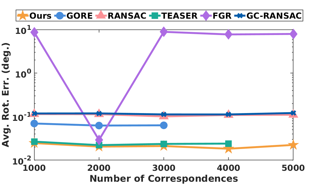
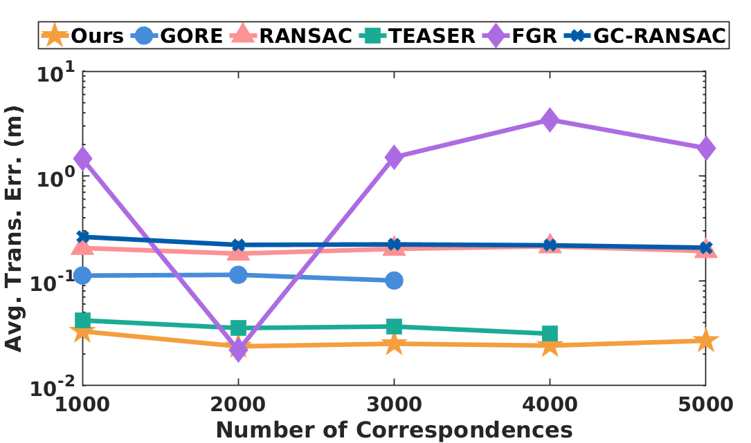
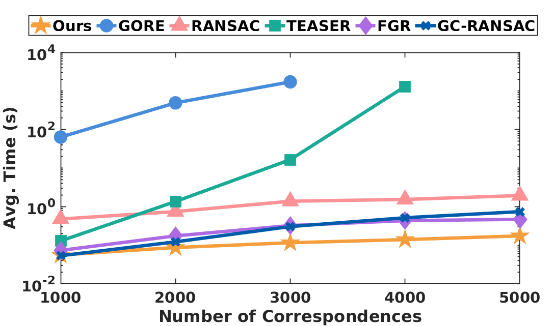
(a) Average rotation error	(b) Average translation error	(c) Average running time

Figure 5: Controlled experiments with $N=\{1000,2000,\dots,5000\}$. The results include average rotation errors, average translation errors, and average running times.

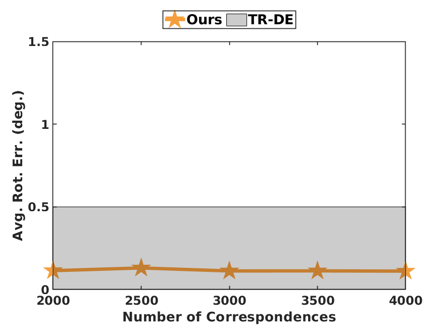
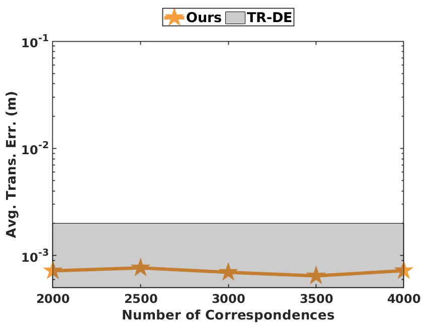
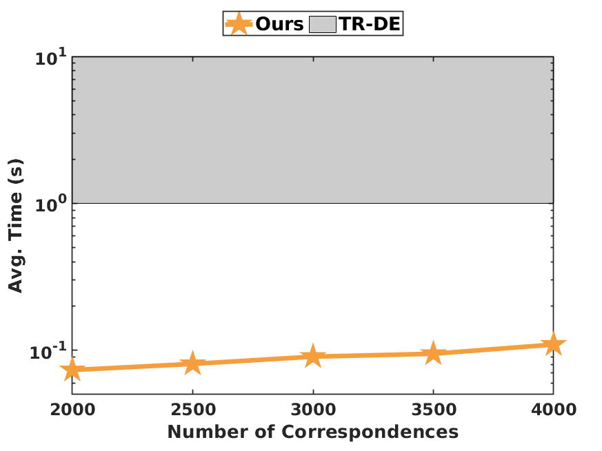
(a) Average rotation error	(b) Average translation error	(c) Average running time

Figure 6: Controlled experiments with the same experimental conditions as TR-DE[31]. The results include average rotation errors, average translation errors, and average running times.

TABLE I: Controlled experiments with the extremely high number of correspondences. The results include average rotation error ($\degree$) $|$ average translation error ($\mathrm{m}$) $|$ average running time (s). Bolded and underlined fonts indicate the first two best values.

Number of correspondences	$10k$	$20k$	$50k$	$100k$	$200k$	$500k$
GORE[13]	$>$1 hour
TEASER[12]	out-of-memory
RANSAC[40]	0.121$|$0.152$|$4.506	0.086$|$0.185$|$6.732	0.073$|$0.153$|$12.51	0.079$|$0.137$|$30.13	0.080$|$0.143$|$92.37	4.961$|$4.883$|$315.7
GC-RANSAC[14]	0.111$|$0.176$|$2.636	0.100$|$0.200$|$9.976	122.4$|$141.3$|$20.64	139.3$|$142.0$|$20.64	126.3$|$138.4$|$20.64	133.4$|$148.5$|$20.64
FGR[9]	0.021$|$0.010$|$1.540	0.024$|$0.013$|$2.477	0.037$|$0.022$|$6.346	0.031$|$0.018$|$12.13	0.024$|$0.018$|$23.97	0.047$|$0.025$|$68.74
Ours	0.016$|$0.017$|$0.397	0.022$|$0.028$|$0.649	0.025$|$0.025$|$1.649	0.025$|$0.028$|$2.963	0.023$|$0.027$|$6.111	0.018$|$0.025$|$15.56

5.1 Experimental Setting

We denote the proposed method as Ours. The compared methods for correspondence-based registration are as follows,

• GORE[13]: A guaranteed outlier removal registration method based on BnB and pose decoupling. It is implemented in C++.

• RANSAC[40]: A typical consensus maximization registration approach implemented in Matlab. The maximum number of iterations is set to $10^{4}$.

• TEASER[12]: A certifiable decoupling-based registration method with a robust cost function. It is implemented in C++.

• FGR[9]: A fast registration method with a robust cost function. It is implemented in C++.

• GC-RANSAC[14]: A variant of RANSAC-based registration method with improvements in local optimization. It is implemented in C++, and the maximum number of iterations is set to $10^{4}$.

• TR-DE[31]: A deterministic point cloud registration method based on BnB and pose decoupling. It is implemented in C++.

• DGR[51]: A learning-based outlier rejection method for point cloud registration. It is implemented in Python.

• PointDSC[52]: A learning-based outlier rejection method for point cloud registration. It is implemented in Python.

Besides, the compared methods for SPCR are as follows,

• GO-ICP[11]: A 6-DOF global optimal registration method based on BnB. It is implemented in C++.

• GO-ICPT: A variant of GO-ICP with outlier trimming and the trimming fraction is set to $10\%$.

• ICP[10]: A typical EM-type method implemented by pcregistericp function in MATLAB.

• CPD[45]: A robust GMM-based registration approach implemented in C.

• GMMReg[46]: A robust and general GMM-based registration method implemented in C.

Similar to [12, 31, 52], the evaluation metrics for point cloud registration in this study include 1) rotation error $E_{\bm{R}}$, 2) translation error $E_{\bm{t}}$, 3) running time, 4) success rate $SR$, and 5) $F1$-score. The error definitions are as follows:

$$E_{\bm{R}}=\arccos{\left(\frac{Tr(\bm{R}_{gt}^{-1}\bm{R}^{*})-1}{2}\right)},$$ (32a)

$$E_{\bm{t}}=\|\bm{t}_{gt}-\bm{t}^{*}\|,$$ (32b)

where $\bm{t}_{gt}$ and $\bm{R}_{gt}$ are the ground truth, $\bm{t}^{*}$ and $\bm{R}^{*}$ are the estimated solutions, and $Tr(\cdot)$ is the trace of a matrix. The successful cases must satisfy the predefined threshold for $E_{\bm{R}}$ and $E_{\bm{t}}$. Besides, the definition of $F1$-score is given in [52].

5.2 Synthetic Data Experiments

In this section, we conduct various experiments on synthetic data to compare the performance of the proposed method with state-of-the-art correspondence-based and correspondence-free registration methods.

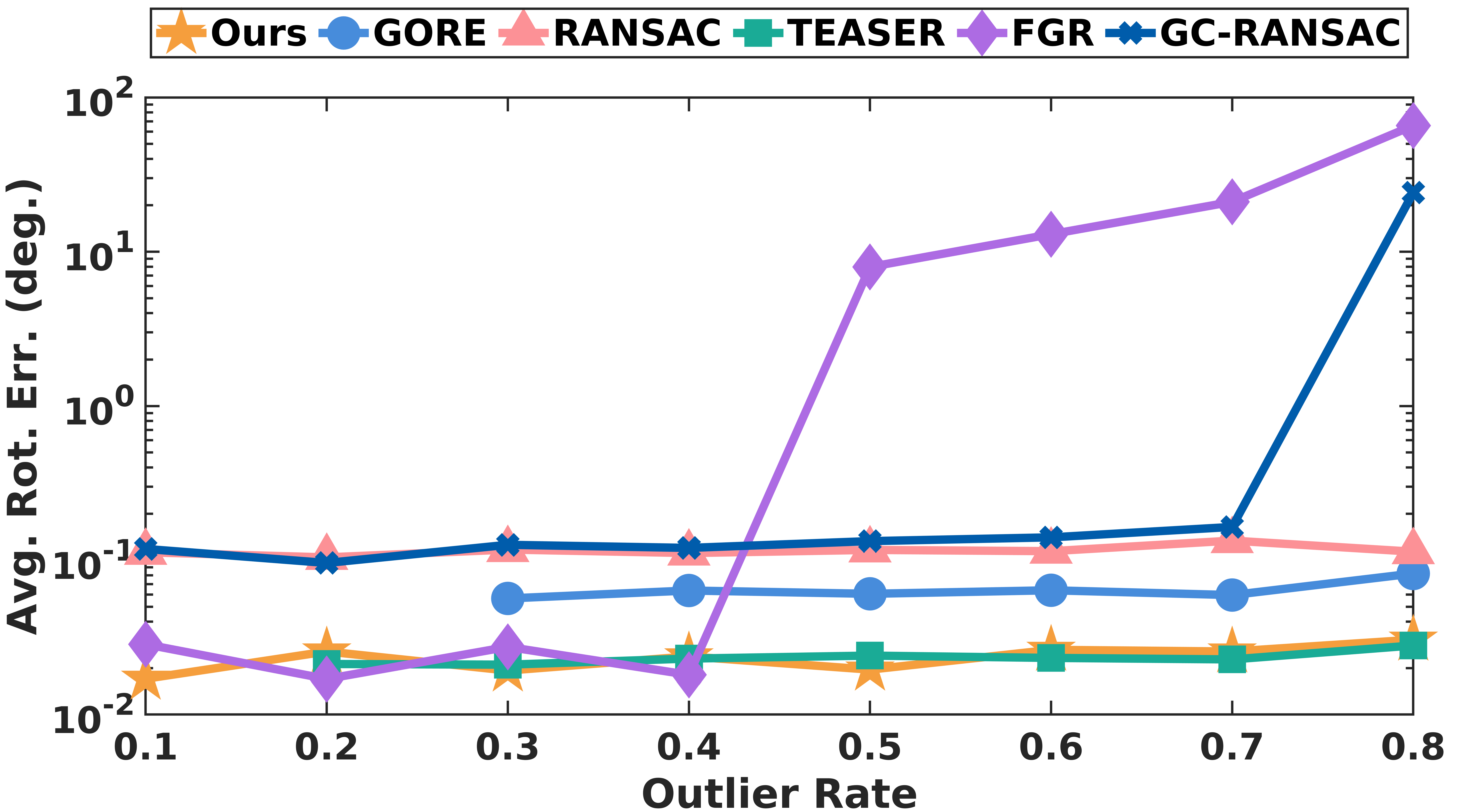
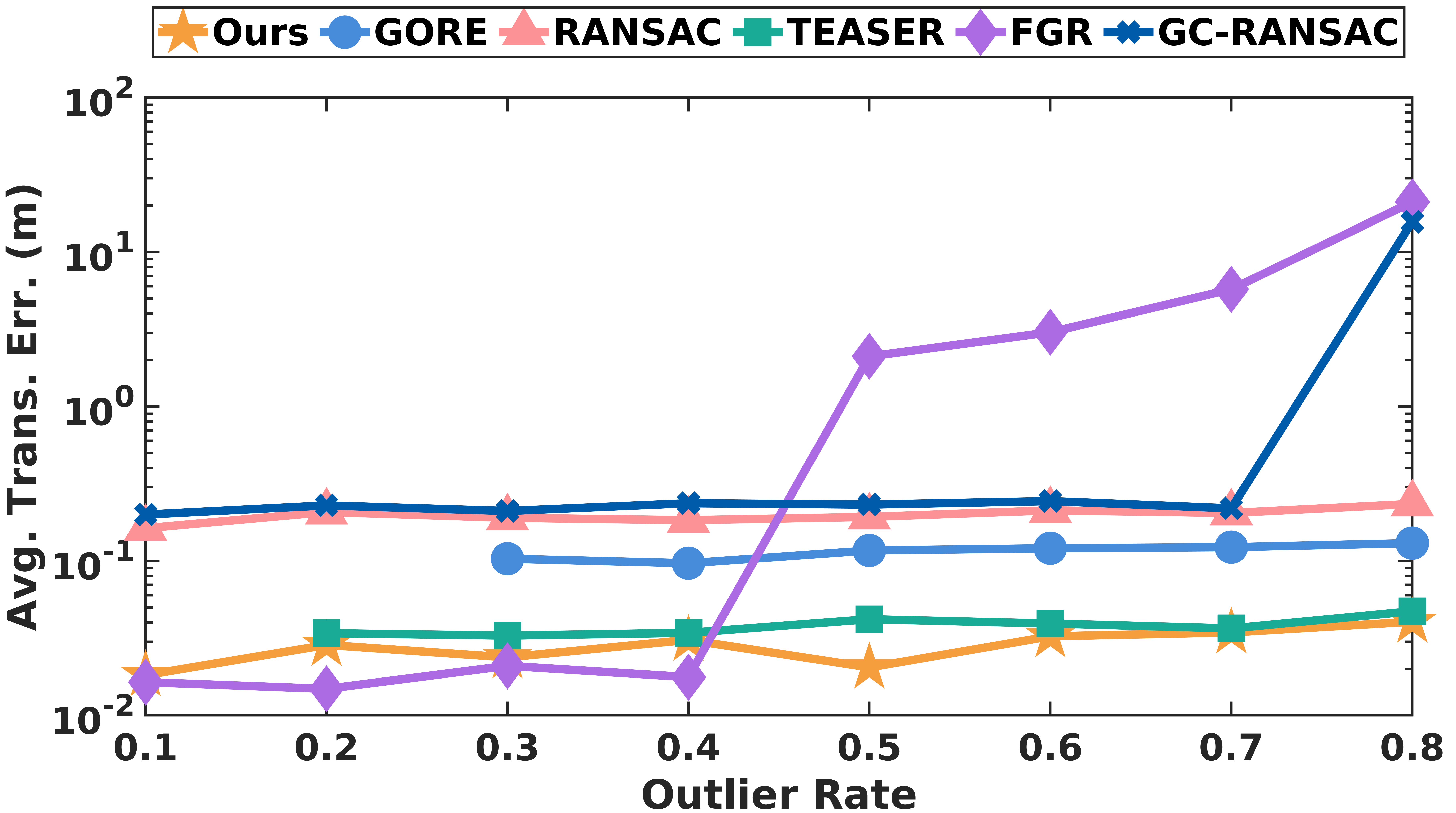
(a) Average rotation error	(b) Average translation error	(c) Average running time

Figure 7: Controlled experiments with $\eta=\{0.1,0.2,\dots,0.8\}$. The results include average rotation errors, average translation errors, and average running times.

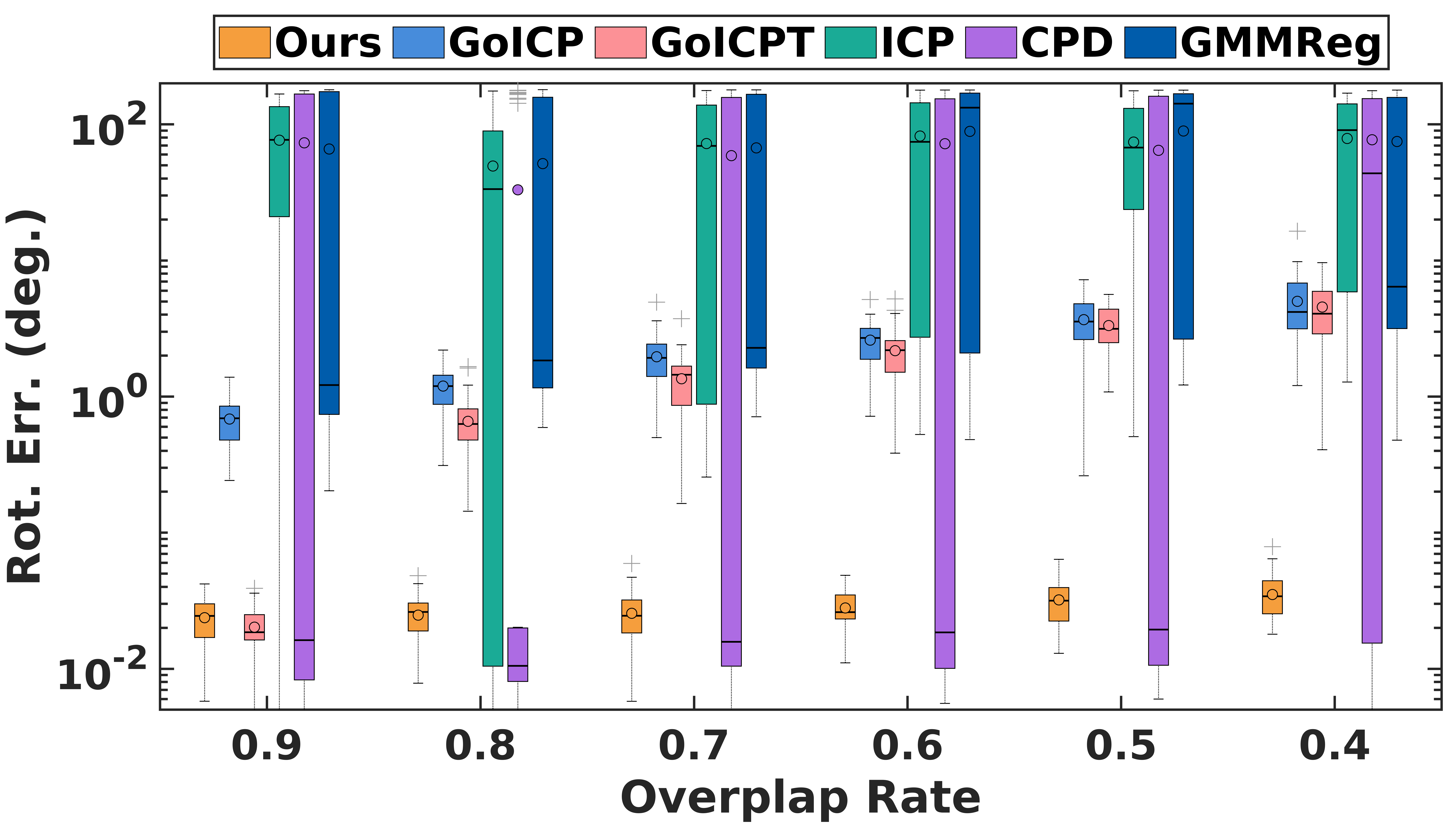
(a) Rotation error	(b) Translation error	(c) Average running time

Figure 8: Controlled SPCR experiments with $\rho=\{0.9,0.8,\dots,0.4\}$. The results include rotation errors, translation errors, and average running times.

5.2.1 Data generation

Firstly, we randomly generate the source point cloud $\mathcal{P}$ in the cube $[-100,100]^{3}$. The source point cloud is transformed by a random rotation $\bm{R}_{gt}\in\mathbb{SO}(3)$ and a random translation $\bm{t}_{gt}\in[-100,100]^{3}$ to generate the target point cloud $\mathcal{Q}$. Then a portion of the points in the target point cloud is replaced by arbitrarily generated points to simulate outliers. The outlier rate $\eta$ is the ratio of these replaced points to all points. Besides, zero-mean Gaussian noise with standard deviation $\sigma$ is added to the target point cloud. Notably, the inlier threshold in each synthetic data experiment is set according to the standard deviation of the noise.

5.2.2 Efficiency and accuracy experiments

This section presents three sets of experiments comparing the efficiency and accuracy of Ours with GORE, RANSAC, TEASER, FGR, GC-RANSAC, and TR-DE. Rotation errors, translation errors, and time costs are recorded for each experiment group. The first group focuses on experiments with a regular number of correspondences. We randomly generate $N=\{1000,2000,\dots,5000\}$ correspondences with a noise level of $\sigma=0.5$ and an outlier rate of $\eta=0.5$. The experiment is repeated $50$ times for each setting, and the average results are depicted in Fig. 5. It is worth noting that results are not reported when the running time exceeds $1800$ seconds. Among the deterministic methods, GORE and TEASER exhibit relatively high accuracy. However, their time costs increase significantly as the number of correspondences grows, with TEASER being the fastest in this regard. FGR, on the other hand, demonstrates occasional unsuccessful results but shows high efficiency. RANSAC and GC-RANSAC suffer from lower accuracy due to sampling uncertainty. Nevertheless, they exhibit relatively high efficiency at the regular outlier rate ($\eta=0.5$). In contrast, Ours outperforms all other methods in terms of both efficiency and accuracy. Notably, when $N$ reaches $4000$, Ours is approximately $10^{4}$ times faster than GORE and TEASER. This may be explained by the reason that even after outlier rejection, a significant number of candidate inlier correspondences are still retained when dealing with a large number of correspondences. Consequently, the optimization process for GORE and TEASER becomes slower.

Since the code of TR-DE[31] is not released publicly, we set the same experimental conditions as TR-DE to compare the performance, which is the second group of experiments. Specifically, the source point cloud is randomly generated within the unit cube, and the experiment is conducted with $N=\{2000,2500,\dots,4000\}$, $\sigma=0.005$, and, $\eta=0.55$. We also conduct $200$ independent trials for each setting and record the average experiment results, as shown in Fig. 6. We use the gray rectangular region to approximately represent the results of TR-DE given in [31]. We can observe that, Ours is about $10$ times faster than TR-DE while keeping comparable accuracy.

To further investigate the potential efficiency advantages of Ours, we conduct the third group of experiments, specifically focusing on extremely high numbers of correspondences: $N=\{10k,20k,50k,100k,200k,500k\}$ (where $k$ denotes one thousand). The remaining settings are consistent with those of the first group. Table I presents the average rotation errors, average translation errors, and average time costs of each method. GORE’s running time exceeds one hour starting from $N=10k$, thus its results are not reported. Furthermore, TEASER demands a substantial amount of memory space, which renders it unable to operate efficiently under such extreme experimental conditions. As $N$ increases to $500k$, RANSAC yields numerous unsatisfactory solutions and incurs a time cost of up to $315.7$s. Additionally, GC-RANSAC fails to converge to the correct result after $N$ reaches $50k$ due to early termination. In comparison to FGR, Ours delivers more accurate rotation estimates but slightly less accurate translation estimates. However, experimental results indicate that the number of correspondences has a relatively minor impact on the efficiency of our method. For instance, when the number of correspondences increases from $10k$ to $500k$, Ours is approximately $8$ to $20$ times faster than RANSAC and roughly $4$ times faster than FGR. Overall, the proposed method exhibits superior efficiency while maintaining competitive accuracy compared to state-of-the-art approaches.

5.2.3 Robustness experiments

In this section, we conduct a group of controlled experiments to compare the robustness of Ours with GORE, RANSAC, TEASER, FGR, and GC-RANSAC. We randomly generate $N=2000$ correspondences with varying outlier rates $(\eta=\{0.1,0.2,\dots,0.8\})$ and a noise level of $\sigma=0.5$. The average rotation errors, average translation errors, and average time costs for each method are reported in Fig. 7. Results beyond a running time of $1800$ seconds are not recorded in this group of experiments. Comparing the registration errors demonstrates that Ours, GORE, RANSAC, and TEASER are robust against up to $80\%$ outlier rates. RANSAC has relatively higher registration errors compared to Ours, GORE, and TEASER. Moreover, the running time of RANSAC increases significantly with an increase in the outlier rate. In contrast, both GORE and TEASER display a significant decrease in running times as the outlier rate increases, due to a corresponding reduction in the number of inliers. This indicates that, for GORE and TEASER, the time required for outlier removal is considerably smaller compared to the time spent on the optimization part. Consequently, they exhibit lower efficiency at regular outlier rates (e.g., $\eta\leq 0.5$). On the other hand, despite the high efficiency exhibited by both the deterministic FGR and the non-deterministic GC-RANSAC, they do not perform well when confronted with high outlier rates (e.g., $\eta\geq 0.7$). In contrast, Ours stands out as one of the fastest and most robust methods.

5.2.4 Challenging SPCR experiments

In this section, we evaluate the performance of our extended simultaneous pose and correspondence registration (SPCR) method against GoICP, GoICPT, ICP, CPD, and GMMReg using the Bunny dataset[20]. The Bunny dataset consists of $35947$ points, and is pre-normalized to fit within the cube $[-1,1]^{3}$, as required by GoICP[11]. Similar to [12], we down-sample the Bunny dataset to $M=100$ points, which serve as the source point cloud $\mathcal{P}$. To generate the target point cloud $\mathcal{Q}$, we apply a random rotation and translation to the source point cloud. Additionally, we randomly remove a certain proportion of points from $\mathcal{Q}$ to simulate partial overlap between $\mathcal{P}$ and $\mathcal{Q}$. The visualization results for a pair of synthetic data are shown in Fig. 1(d-1), where the bolded points represent the down-sampled point clouds. Furthermore, we add zero-mean Gaussian noise with $\sigma=0.001$ to the source point cloud $\mathcal{P}$. The registration experiment is repeated $50$ times for each overlap rate in $\rho=\{0.9,0.8,\dots,0.4\}$.

The registration errors and average running times for each approach are presented in Fig. 8. During repeated experiments, the local methods, ICP, CPD, and GMMReg, exhibit a tendency to converge to local optima, resulting in incorrect results. However, their efficiency remains a notable advantage. In contrast, the global methods GoICP and its variant GoICPT demonstrate greater robustness compared to these local methods. In particular, GoICPT with a $10\%$ trimming ratio achieves significantly higher accuracy at an overlap rate of $0.1$. Nevertheless, these global methods suffer from relatively slow running times, which increase more rapidly than our proposed method. Consequently, when the overlap ratio is low (e.g., $\rho\leq 0.7$), Ours is faster than GoICP and GoICPT. As a global method, Ours also falls short in terms of efficiency compared to the local methods. However, Ours is more robust than local methods ICP, CPD, and GMMReg. Furthermore, as depicted in Fig. 1(d), Ours exhibits greater robustness than ICP and higher efficiency than GoICP on a randomly generated pair of Bunny data ($\rho=0.6$). These experiments illustrate the potential practicality of our proposed approach in addressing the challenging SPCR problem and its strength in terms of robustness and efficiency.

5.3 Real-World Data Experiments

To assess the performance of the proposed method on real-world data, we utilize the Bremen dataset[17], ETH dataset[18], and KITTI dataset[19] in this section. These datasets present challenging outdoor LiDAR scenarios, with the former two captured using terrestrial LiDAR and the latter collected from onboard LiDAR.

5.3.1 Bremen dataset experiments

TABLE II: Detailed information about the Bremen Dataset.

Scan pair	Number of points ($10^{6}$)	Number of key-points	Number of correspondences	Outlier rate
s1-s0	16.16-15.90	30328-30290	5001	98.54%
s2-s0	15.25-15.90	39368-30290	6303	99.64%
s3-s2	15.03-15.25	43856-39368	8194	95.08%
s4-s2	18.05-15.25	26581-39368	5393	97.59%
s5-s4	18.76-18.05	20023-26581	4768	91.19%
s6-s5	20.33-18.76	9423-20023	1840	97.34%
s7-s6	18.47-20.33	16608-9423	2554	93.46%
s8-s7	15.85-18.47	19599-16608	3934	94.20%
s9-s7	16.29-18.47	32281-16608	4291	97.48%
s10-s9	15.18-16.29	36689-32281	8662	90.67%
s11-s9	14.61-16.29	37187-32281	7563	96.50%
s12-s10	15.76-15.18	36084-36689	8214	92.62%

TABLE III: Detailed information about the ETH Dataset.

Scan pair	Number of points ($10^{6}$)	Number of key-points	Number of correspondences	Outlier rate
Arch1	23.56-30.90	19007-12254	12617	98.45%
Arch2	30.90-29.45	12254-13286	11699	98.77%
Courtyard1	12.71-12.15	9634-12125	15325	86.55%
Courtyard2	12.15-16.75	12125-4081	8069	90.62%
Facade1	25.08-15.25	1586-2810	1901	97.16%
Facade2	15.25-15.79	2810-2215	2368	96.92%
Office1	10.73-10.69	1348-1277	1279	97.65%
Office2	10.69-10.75	1277-1486	1355	98.97%
Trees1	19.63-19.60	10883-10898	9543	99.41%
Trees2	20.39-20.48	12542-12522	11253	97.87%

(a) Rotation error

(b) Translation error

(c) Running time

Figure 9: Experiment results on the Bremen dataset[17] with the FPFH [15] descriptor. The results include rotation errors, translation errors, and running times.

Figure 10: Complete registration results of Ours on the Bremen dataset[17], where different scans are indicated by different colors. The pair-wise point cloud registration is conducted for all $12$ scan pairs.

(a) Rotation error

(b) Translation error

(c) Running time

Figure 11: Experiment results on the ETH dataset[18] with the FPFH [15] descriptor. The results include rotation errors, translation errors, and running times.

The Bremen dataset[17] is a large-scale outdoor dataset with $13$ LiDAR scans. Similar to [4, 7], we initially down-sample the scans using the voxel grid algorithm[53]. Subsequently, we extract ISS [54] key-points and calculate FPFH [15] descriptors for each key-point. Through K-nearest neighbor search, we generate the set of putative correspondences $\mathcal{K}$. The ground-truth pose for each scan is provided within the dataset. Since the proposed method is only for pair-wise registration, we construct $12$ scan pairs to register all scans. Table II provides detailed information for each scan pair from the Bremen dataset, including the number of points, number of key-points, number of correspondences, and outlier rate. The down-sampling resolution for the Bremen dataset is set to $0.15$\mathrm{m}$$, which also determines the inlier threshold. With several thousand correspondences, the outlier rate ranges from approximately $90\%$ to $99\%$ for the Bremen dataset. We employ the proposed method (Ours), as well as GORE, RANSAC, TEASER, FGR, and GC-RANSAC, to register these scan pairs.

We compare the rotation error, translation error, and running time of each method for each scan pair, as shown in Fig. 9. Notably, when dealing with the registration of the s2-s0 scan pair, all compared methods, except for Ours, fail due to the exceptionally high outlier rate ($99.64\%$). GORE and TEASER demonstrate successful alignment for the remaining scan pairs with relatively high accuracy. Despite this, GORE exhibits the highest time cost among all methods, even when the number of correspondences is small or the outlier rate is low, consistent with the findings from synthetic data experiments. For instance, in the case of the s10-s9 pair, which only has a $90.67\%$ outlier rate, GORE requires over $3$ hours for alignment, while TEASER takes up to $26.84$ seconds. In contrast, Ours achieves registration in a mere $0.342$ seconds. Furthermore, Fig.1(a) shows another registration case for the s8-s7 scan pair, where Ours not only achieves superior accuracy but also is approximately $10^{3}$ times faster than GORE and about $4$ times faster than TEASER.

On the other hand, RANSAC demonstrates unstable performance, occasionally generating unsatisfactory solutions with significant registration errors, as observed in pairs s1-s0, s2-s0, s4-s2, and s9-s7. Moreover, RANSAC is also time-consuming in these practical scenarios with high outlier rates and a large number of correspondences. FGR, while fast for all scan pairs, often converges to erroneous results. Although GC-RANSAC outperforms RANSAC in terms of stability and efficiency, it still struggles to successfully register all scan pairs. In contrast, Ours exhibits remarkable robustness, achieving a $100\%$ registration success rate on the Bremen dataset. Furthermore, Ours shows higher efficiency compared to GORE and TEASER, which exhibit similar levels of robustness and accuracy as Ours.

5.3.2 ETH dataset experiments

The ETH dataset[18] is a challenging large-scale LiDAR dataset that encompasses five distinct scenarios: Arch, Courtyard, Facade, Office, and Trees. The average overlap rates of these scenarios are $30-40\%,40-70\%,60-70\%,\textgreater 80\%,\approx 50\%$, respectively, as reported in [7]. To ensure the generality of the registration algorithm, we select two scan pairs from each scenario for our registration experiments. The ETH dataset provides ground truth information regarding the relative pose, enabling accurate evaluation. We follow the same data preparation strategy outlined in Section 5.3.1 to establish the initial correspondence set $\mathcal{K}$. For the ETH dataset, the down-sampling resolution and the inlier threshold are both set to $0.1$\mathrm{m}$$. Detailed information about the ETH dataset, including the number of points, number of key-points, number of correspondences, and outlier rate, can be found in Table III. The outlier rate in the ETH dataset ranges from approximately $86\%$ to $99\%$, with the number of correspondences varying from around $1k$ to $15k$. To evaluate the registration performance, we compare Ours, GORE, RANSAC, TEASER, FGR, and GC-RANSAC using a total of 10 scan pairs from the ETH dataset.

Fig. 11 reports the rotation error, translation error, and running time for each method evaluated on the ETH dataset. Ours, GORE, and TEASER achieve remarkable robustness over all five scenes, successfully registering all scan pairs. GORE exhibits better accuracy overall compared to Ours, although it is time-consuming. Nevertheless, the registration errors achieved by Ours are still acceptable for practical applications. While the overall accuracy of TEASER is lower than that of Ours and GORE, its time cost increases significantly when dealing with a large number of inliers. For instance, Ours is approximately $280$ times faster than TEASER in aligning the scan pair Courtyard1 with an outlier rate of $86.55\%$, and about $42$ times faster than TEASER in aligning the scan pair Courtyard2 with an outlier rate of $90.62\%$. Another registration case for the scan pair Arch1 is illustrated in Fig. 1(b), where Ours achieves the lowest translation error and is roughly $480$ times faster than GORE and about $4$ times faster than TEASER. The visualization results of the proposed method for the remaining four scenarios are provided in Fig. 12. Similar to the results in Section 5.3.1, FGR and GC-RANSAC demonstrate relatively high efficiency but exhibit instability when registering scan pairs with high outlier rates. RANSAC is not only time-consuming on the ETH dataset, but also prone to producing incorrect registration results. In summary, benefiting from the pose decoupling strategy based on residual projections, the proposed registration method is more efficient than the state-of-the-art methods while ensuring superior robustness.

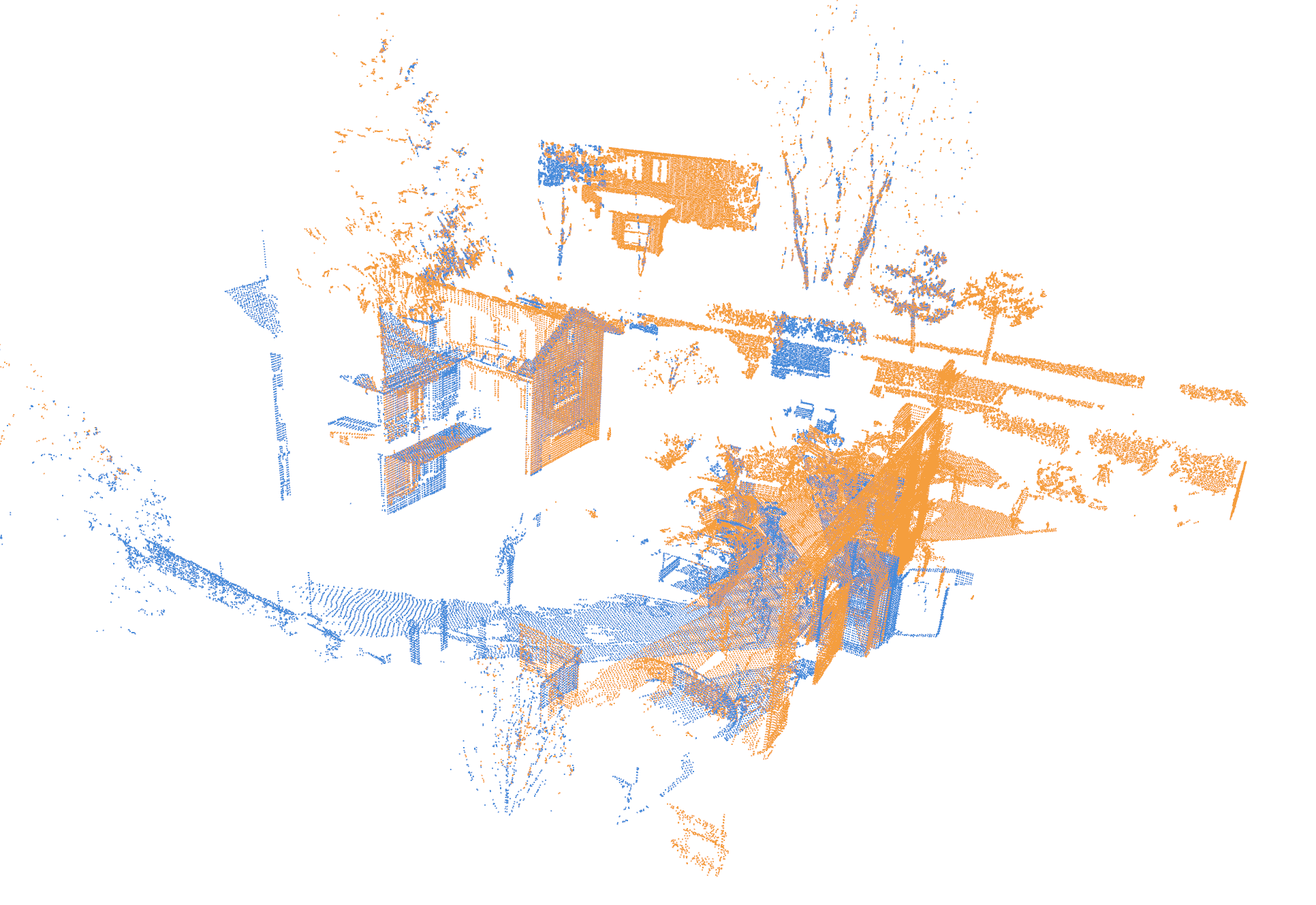
(a) Courtyard1	(b) Facade1
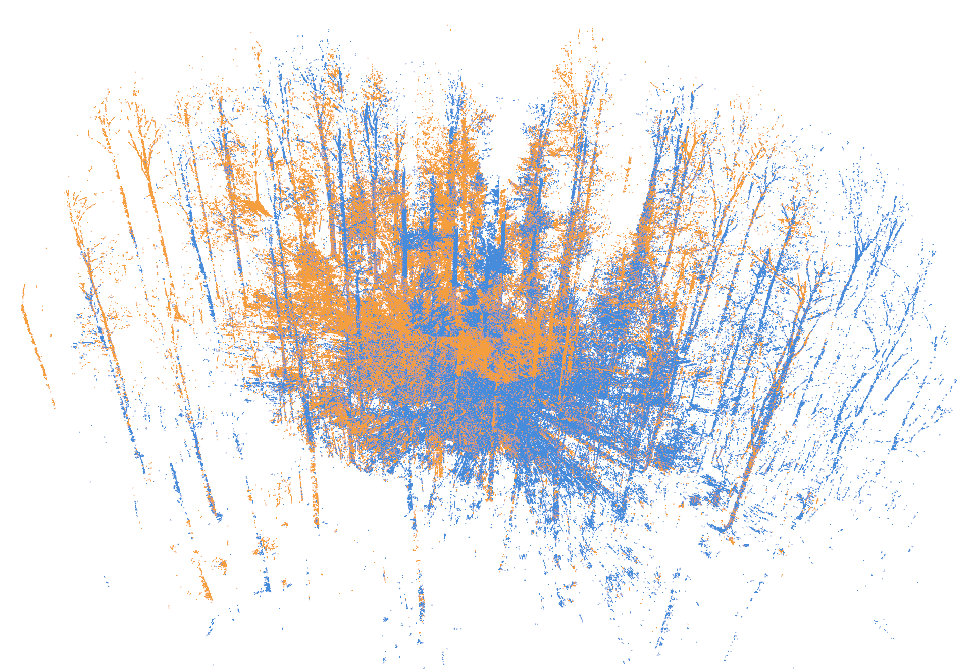
(c) Office1	(b) Trees1

Figure 12: Registration results of the proposed method on the ETH dataset[18], including four scan pairs: (a) Courtyard1, (b) Facade1, (c) Office1, and (d) Trees1. The aligned source point cloud is blue, and the target point cloud is yellow.

5.3.3 KITTI dataset experiments

TABLE IV: Experiment results on the KITTI dataset[19] with FCGF [16] descriptors. Bolded and underlined fonts indicate the first two best values.

Method	$SR$(%)	$E_{\bm{R}}$(°)	$E_{\bm{t}}$(cm)	$F1$(%)	Time(s)
RANSAC[40]	96.40	0.36	21.12	84.77	2.56
TEASER[12]	95.50	0.33	22.38	85.77	31.46
FGR[9]	96.94	0.34	19.69	85.80	0.99
GC-RANSAC[14]	97.48	0.32	20.68	85.42	1.16
TR-DE[31]	98.20	0.38	18.00	85.99	3.01
DGR[51]	95.14	0.43	23.28	73.60	0.86
PointDSC[52]	97.84	0.33	20.99	85.29	0.31
Ours	98.20	0.32	20.05	86.40	0.62

Following the data preparation strategy in [31, 52, 16], we evaluate the performance of the proposed method on the KITTI dataset[19]. The initial correspondences are generated using the learning-based descriptor FCGF[16], and the inlier threshold is set to $0.6$\mathrm{m}$$. For successful registration, we set the thresholds for rotation error ($E_{\bm{R}}$) and translation error ($E_{\bm{t}}$) to $5\degree$ and $0.6$\mathrm{m}$$, respectively. In addition to comparing the performance of Ours against traditional methods such as RANSAC, TEASER, FGR, GC-RANSAC, and TR-DE, we also compare it with learning-based methods, including DGR[51] and PointDSC[52]. Notably, the learning-based descriptor FCGF outperforms traditional descriptors, resulting in a relatively low outlier rate for FCGF-based correspondences (approximately $58.7\%$ on average). Consequently, GORE is significantly slow on the KITTI dataset, and therefore, we do not report its results.

As shown in Table IV, the success rate of all methods is over $95\%$ due to the low outlier rate of FCGF-based correspondences. Among these methods, Ours achieves the highest success rate of $98.20\%$ as well as TR-DE. Although Ours is not the most efficient method, it ranks second in terms of efficiency among all methods. For instance, Ours is approximately $5$ times faster than the BnB-based TR-DE, about $4$ times faster than the non-deterministic RANSAC, and approximately $50$ times faster than the deterministic TEASER. It is worth mentioning that the most efficient method is the learning-based registration method PointDSC. However, learning-based methods often require additional training procedures and may perform well only on the datasets they were trained on. Additionally, Ours exhibits the best rotation accuracy and $F1$-score. Fig. 1(c) provides an example of registering a selected pair from the KITTI dataset, where Ours has better accuracy and efficiency than FGR and GC-RANSAC. In general, compared to the state-of-the-art methods, including learning-based methods, Ours demonstrates competitive performance in efficiency and even better performance in robustness. This demonstrates the effectiveness of both the pose decoupling strategy and the BnB-based search method in our proposed method.

6 Conclusion

In this paper, we present an efficient and deterministic point cloud registration method, leveraging a novel pose decoupling strategy. By utilizing $L_{\infty}$ residual projections, we successfully decouple the initial 6-DOF problem into three 2-DOF sub-problems, resulting in improved efficiency. Furthermore, we introduce a step-wise search strategy based on branch and bound for these sub-problems. Specifically, we define the inlier set maximization objective function and derive the novel upper bound based on the interval stabbing technology. Interestingly, thanks to its significant robustness, our proposed method can be extended to solve the challenging SPCR problem by introducing the interval merging technology. Extensive experiments conducted on both synthetic and real-world datasets demonstrate the superior performance of our proposed method in terms of efficiency and robustness when compared to state-of-the-art approaches.

References

- [1] M. Zhao, L. Ma, X. Jia, D.-M. Yan, and T. Huang, “Graphreg: Dynamical point cloud registration with geometry-aware graph signal processing,” IEEE Transactions on Image Processing, vol. 31, pp. 7449–7464, 2022.
- [2] X. Li, Y. Liu, V. Lakshminarasimhan, H. Cao, F. Zhang, and A. Knoll, “Globally optimal robust radar calibration in intelligent transportation systems,” IEEE Transactions on Intelligent Transportation Systems, pp. 1–14, 2023.
- [3] G. Blais and M. D. Levine, “Registering multiview range data to create 3d computer objects,” IEEE Transactions on Pattern Analysis and Machine Intelligence, vol. 17, no. 8, pp. 820–824, 1995.
- [4] J. Li, “A practical o(n2) outlier removal method for correspondence-based point cloud registration,” IEEE Transactions on Pattern Analysis and Machine Intelligence, vol. 44, no. 8, pp. 3926–3939, 2022.
- [5] D. Cattaneo, M. Vaghi, and A. Valada, “Lcdnet: Deep loop closure detection and point cloud registration for lidar slam,” IEEE Transactions on Robotics, vol. 38, no. 4, pp. 2074–2093, 2022.
- [6] J. Zhang and S. Singh, “Visual-lidar odometry and mapping: Low-drift, robust, and fast,” in 2015 IEEE International Conference on Robotics and Automation (ICRA). IEEE, 2015, pp. 2174–2181.
- [7] J. Li, P. Shi, Q. Hu, and Y. Zhang, “Qgore: Quadratic-time guaranteed outlier removal for point cloud registration,” IEEE Transactions on Pattern Analysis and Machine Intelligence, pp. 1–16, 2023.
- [8] H. Li and R. Hartley, “The 3d-3d registration problem revisited,” in 2007 IEEE 11th international conference on computer vision. IEEE, 2007, pp. 1–8.
- [9] Q.-Y. Zhou, J. Park, and V. Koltun, “Fast global registration,” in European conference on computer vision. Springer, 2016, pp. 766–782.
- [10] P. Besl and N. D. McKay, “A method for registration of 3-d shapes,” IEEE Transactions on Pattern Analysis and Machine Intelligence, vol. 14, no. 2, pp. 239–256, 1992.
- [11] J. Yang, H. Li, D. Campbell, and Y. Jia, “Go-icp: A globally optimal solution to 3d icp point-set registration,” IEEE Transactions on Pattern Analysis and Machine Intelligence, vol. 38, no. 11, pp. 2241–2254, 2016.
- [12] H. Yang, J. Shi, and L. Carlone, “Teaser: Fast and certifiable point cloud registration,” IEEE Transactions on Robotics, vol. 37, no. 2, pp. 314–333, 2020.
- [13] A. P. Bustos and T.-J. Chin, “Guaranteed outlier removal for point cloud registration with correspondences,” IEEE transactions on pattern analysis and machine intelligence, vol. 40, no. 12, pp. 2868–2882, 2017.
- [14] D. Barath and J. Matas, “Graph-cut ransac: Local optimization on spatially coherent structures,” IEEE Transactions on Pattern Analysis and Machine Intelligence, vol. 44, no. 9, pp. 4961–4974, 2021.
- [15] R. B. Rusu, N. Blodow, and M. Beetz, “Fast point feature histograms (fpfh) for 3d registration,” in 2009 IEEE international conference on robotics and automation. IEEE, 2009, pp. 3212–3217.
- [16] C. Choy, J. Park, and V. Koltun, “Fully convolutional geometric features,” in Proceedings of the IEEE/CVF international conference on computer vision, 2019, pp. 8958–8966.
- [17] D. Borrmann, J. Elseberg, and A. Nüchter, “Thermal 3d mapping of building façades,” in Intelligent Autonomous Systems 12: Volume 1 Proceedings of the 12th International Conference IAS-12, held June 26-29, 2012, Jeju Island, Korea. Springer, 2013, pp. 173–182.
- [18] P. W. Theiler, J. D. Wegner, and K. Schindler, “Keypoint-based 4-points congruent sets–automated marker-less registration of laser scans,” ISPRS journal of photogrammetry and remote sensing, vol. 96, pp. 149–163, 2014.
- [19] A. Geiger, P. Lenz, and R. Urtasun, “Are we ready for autonomous driving? the kitti vision benchmark suite,” in 2012 IEEE conference on computer vision and pattern recognition. IEEE, 2012, pp. 3354–3361.
- [20] B. Curless and M. Levoy, “A volumetric method for building complex models from range images,” in Proceedings of the 23rd annual conference on Computer graphics and interactive techniques, 1996, pp. 303–312.
- [21] S. Huang, Z. Gojcic, M. Usvyatsov, A. Wieser, and K. Schindler, “Predator: Registration of 3d point clouds with low overlap,” in Proceedings of the IEEE/CVF Conference on computer vision and pattern recognition, 2021, pp. 4267–4276.
- [22] L. Yan, P. Wei, H. Xie, J. Dai, H. Wu, and M. Huang, “A new outlier removal strategy based on reliability of correspondence graph for fast point cloud registration,” IEEE Transactions on Pattern Analysis and Machine Intelligence, 2022.
- [23] H. Li, “Consensus set maximization with guaranteed global optimality for robust geometry estimation,” in 2009 IEEE 12th International Conference on Computer Vision, 2009, pp. 1074–1080.
- [24] D. Campbell, L. Petersson, L. Kneip, and H. Li, “Globally-optimal inlier set maximisation for camera pose and correspondence estimation,” IEEE transactions on pattern analysis and machine intelligence, vol. 42, no. 2, pp. 328–342, 2018.
- [25] H. Le, T.-J. Chin, A. Eriksson, T.-T. Do, and D. Suter, “Deterministic approximate methods for maximum consensus robust fitting,” IEEE transactions on pattern analysis and machine intelligence, vol. 43, no. 3, pp. 842–857, 2019.
- [26] R. I. Hartley and F. Kahl, “Global optimization through rotation space search,” International Journal of Computer Vision, vol. 82, no. 1, pp. 64–79, 2009.
- [27] D. Campbell and L. Petersson, “Gogma: Globally-optimal gaussian mixture alignment,” in Proceedings of the IEEE conference on computer vision and pattern recognition, 2016, pp. 5685–5694.
- [28] A. P. Bustos, T.-J. Chin, A. Eriksson, H. Li, and D. Suter, “Fast rotation search with stereographic projections for 3d registration,” IEEE Transactions on Pattern Analysis and Machine Intelligence, vol. 38, no. 11, pp. 2227–2240, 2016.
- [29] J. Straub, T. Campbell, J. P. How, and J. W. Fisher, “Efficient global point cloud alignment using bayesian nonparametric mixtures,” in Proceedings of the IEEE Conference on Computer Vision and Pattern Recognition, 2017, pp. 2941–2950.
- [30] Y. Liu, C. Wang, Z. Song, and M. Wang, “Efficient global point cloud registration by matching rotation invariant features through translation search,” in Proceedings of the European Conference on Computer Vision (ECCV), 2018, pp. 448–463.
- [31] W. Chen, H. Li, Q. Nie, and Y.-H. Liu, “Deterministic point cloud registration via novel transformation decomposition,” in Proceedings of the IEEE/CVF Conference on Computer Vision and Pattern Recognition, 2022, pp. 6348–6356.
- [32] Z. Cai, T.-J. Chin, A. P. Bustos, and K. Schindler, “Practical optimal registration of terrestrial lidar scan pairs,” ISPRS journal of photogrammetry and remote sensing, vol. 147, pp. 118–131, 2019.
- [33] X. Li, Y. Liu, Y. Xia, V. Lakshminarasimhan, H. Cao, F. Zhang, U. Stilla, and A. Knoll, “Fast and deterministic (3+1)dof point set registration with gravity prior,” ISPRS Journal of Photogrammetry and Remote Sensing, vol. 199, pp. 118–132, 2023.
- [34] C. Wang, Y. Liu, Y. Wang, X. Li, and M. Wang, “Efficient and outlier-robust simultaneous pose and correspondence determination by branch-and-bound and transformation decomposition,” IEEE Transactions on Pattern Analysis and Machine Intelligence, pp. 1–1, 2021.
- [35] Y. Jiao, Y. Wang, X. Ding, M. Wang, and R. Xiong, “Deterministic optimality for robust vehicle localization using visual measurements,” IEEE Transactions on Intelligent Transportation Systems, vol. 23, no. 6, pp. 5397–5410, 2022.
- [36] K. Sim and R. Hartley, “Removing outliers using the norm,” in 2006 IEEE Computer Society Conference on Computer Vision and Pattern Recognition (CVPR’06), vol. 1. IEEE, 2006, pp. 485–494.
- [37] F. Kahl and R. Hartley, “Multiple-view geometry under the -norm,” IEEE Transactions on Pattern Analysis and Machine Intelligence, vol. 30, no. 9, pp. 1603–1617, 2008.
- [38] L. Peng, M. C. Tsakiris, and R. Vidal, “Arcs: Accurate rotation and correspondence search,” in Proceedings of the IEEE/CVF Conference on Computer Vision and Pattern Recognition, 2022, pp. 11 153–11 163.
- [39] B. K. Horn, “Closed-form solution of absolute orientation using unit quaternions,” Josa a, vol. 4, no. 4, pp. 629–642, 1987.
- [40] M. A. Fischler and R. C. Bolles, “Random sample consensus: a paradigm for model fitting with applications to image analysis and automated cartography,” Communications of the ACM, vol. 24, no. 6, pp. 381–395, 1981.
- [41] J. Li, Q. Hu, and M. Ai, “Gesac: Robust graph enhanced sample consensus for point cloud registration,” ISPRS Journal of Photogrammetry and Remote Sensing, vol. 167, pp. 363–374, 2020.
- [42] L. Sun, “Ransic: Fast and highly robust estimation for rotation search and point cloud registration using invariant compatibility,” IEEE Robotics and Automation Letters, vol. 7, no. 1, pp. 143–150, 2021.
- [43] D. Barath, J. Noskova, and J. Matas, “Marginalizing sample consensus,” IEEE Transactions on Pattern Analysis and Machine Intelligence, vol. 44, no. 11, pp. 8420–8432, 2021.
- [44] Á. P. Bustos, T. Chin, F. Neumann, T. Friedrich, and M. Katzmann, “A practical maximum clique algorithm for matching with pairwise constraints,” CoRR, vol. abs/1902.01534, 2019. [Online]. Available: http://arxiv.org/abs/1902.01534
- [45] A. Myronenko and X. Song, “Point set registration: Coherent point drift,” IEEE transactions on pattern analysis and machine intelligence, vol. 32, no. 12, pp. 2262–2275, 2010.
- [46] B. Jian and B. C. Vemuri, “Robust point set registration using gaussian mixture models,” IEEE transactions on pattern analysis and machine intelligence, vol. 33, no. 8, pp. 1633–1645, 2010.
- [47] Y. Liu, G. Chen, and A. Knoll, “Globally optimal vertical direction estimation in atlanta world,” IEEE Transactions on Pattern Analysis and Machine Intelligence, vol. 44, no. 4, pp. 1949–1962, 2020.
- [48] Y. Liu, Y. Wang, M. Wang, G. Chen, A. Knoll, and Z. Song, “Globally optimal linear model fitting with unit-norm constraint,” International Journal of Computer Vision, vol. 130, no. 4, pp. 933–946, 2022.
- [49] M. De Berg, M. Van Kreveld, M. Overmars, O. Schwarzkopf, M. de Berg, M. van Kreveld, M. Overmars, and O. Schwarzkopf, Computational Geometry: Introduction. Springer, 1997.
- [50] K. Mehlhorn, P. Sanders, and P. Sanders, Algorithms and data structures: The basic toolbox. Springer, 2008, vol. 55.
- [51] C. Choy, W. Dong, and V. Koltun, “Deep global registration,” in Proceedings of the IEEE/CVF conference on computer vision and pattern recognition, 2020, pp. 2514–2523.
- [52] X. Bai, Z. Luo, L. Zhou, H. Chen, L. Li, Z. Hu, H. Fu, and C.-L. Tai, “Pointdsc: Robust point cloud registration using deep spatial consistency,” in Proceedings of the IEEE/CVF Conference on Computer Vision and Pattern Recognition, 2021, pp. 15 859–15 869.
- [53] R. B. Rusu and S. Cousins, “3d is here: Point cloud library (pcl),” in 2011 IEEE international conference on robotics and automation. IEEE, 2011, pp. 1–4.
- [54] Y. Zhong, “Intrinsic shape signatures: A shape descriptor for 3d object recognition,” in 2009 IEEE 12th international conference on computer vision workshops, ICCV Workshops. IEEE, 2009, pp. 689–696.