Searching for a Heavy Neutral CP-Even Higgs Boson
in the BLSSM at the LHC Run 3 and HL-LHC

Abstract

The detection of a heavy neutral CP-even Higgs boson of the $B-L$ Supersymmetric Standard Model (BLSSM), $h^{\prime}$, with $m_{h^{\prime}}\simeq 400~{}\text{GeV}$, at the Large Hadron Collider (LHC) for a center-of-mass energy of $\sqrt{s}=14~{}\text{TeV}$, is investigated. The following production and decay channels are considered: $gg\to h^{\prime}\to{ZZ}\to 4\ell$ and $gg\to h^{\prime}\to{W^{+}W^{-}}\to 2\ell+\not{E}_{T}$ (with $\not{E}_{T}$ being the Missing Transverse Energy (MET)), where $\ell=e,\mu$, with integrated luminosity $L_{\text{int}}=300~{}{\text{fb}}^{-1}$ (Run 3). Furthermore, we also look into the di-Higgs channel $gg\to h^{\prime}\to{hh}\to{b\bar{b}\gamma\gamma}$ at the High-Luminosity LHC (HL-LHC) with an integrated luminosity of $L_{\text{int}}=3000~{}{\text{fb}}^{-1}$. We demonstrate that promising signals with high statistical significance can be obtained through the three aforementioned channels.

I INTRODUCTION

The search for a heavy neutral CP-even Higgs boson at the current Run 3 of the LHC and a future HL-LHC is an active area of research [1, 2, 3, 4, 5, 6, 7, 8, 9]. This is so because virtually any extension of the Higgs sector beyond the single doublet structure of the Standard Model (SM), in which the only neutral CP-even state of it is identified with the particle that was discovered in 2012 at the LHC by the ATLAS and CMS experiments [10, 11], contains it. As a result, probing such a heavy Higgs boson is one of the main goals of the LHC experiments, as it could well provide the first hint for physics Beyond the SM (BSM). Both ATLAS and CMS have searched for a heavy Higgs boson and the corresponding analyses typically involve looking for events in which the heavy Higgs boson is produced and then decays into SM particles, such as $W^{\pm}$ or $Z$ bosons, in turn decaying into leptons or jets [1], or into the SM Higgs boson itself [12], which then decays into $b$ quarks or $\tau$ leptons.

Supersymmetric extensions of the SM are one of the BSM frameworks that consistently predict the existence of several Higgs bosons, including a heavy neutral CP-even one. Such a Higgs boson mass can be significantly larger than the one of the SM Higgs state, potentially reaching several hundred GeV. For example, the Minimal Supersymmetric Standard Model (MSSM) contains five Higgs bosons: two CP-even ($h$ and $H$, with $m_{h}<m_{H}$), one CP-odd ($A$) and two charged states ($H^{+}$ and $H^{-}$): for reviews, see, e.g., [13]. This is the simplest construct implementing supersymmetry, where the lightest CP-even Higgs boson, $h$, is designated as the SM Higgs boson, with a mass of 125 GeV, which, however, imposes a strenuous configuration on the MSSM parameter space, forcing the other CP-even Higgs boson, $H$, to be rather heavy and significantly decoupled. However, if supersymmetry is non-minimal, in either its gauge or Higgs sector or both, then the mass of additional CP-even Higgs states can become rather less constrained [14]. An example of this is the so-called BLSSM, which indeed offers the possibility of LHC signals for a CP-even Higgs state not only above the SM Higgs mass, e.g., in the range up to 500 GeV [9], but also afford one with a lighter mass spectrum, in turn able to explain past [15, 16] and present data anomalies [17].

The BLSSM is a theoretical extension of the MSSM that includes an additional $U(1)$ gauge symmetry known as $B-L$ (baryon number minus lepton number) [18, 19, 20, 21] as well as an extended Higgs sector. The $B-L$ symmetry is motivated by the observation that the difference between baryon and lepton number is conserved in many particle physics processes. In the BLSSM, the $B-L$ symmetry may be broken at the few TeV scale, giving rise to new particles such as two new extra neutral CP-even Higgs bosons. One of them, labeled $h^{\prime}$, can have energies in the hundreds of GeV range. It is indeed the presence of such a $h^{\prime}$ state that causes the aforementioned new phenomenology to emerge in collider experiments, which can then be used to test the BLSSM hypothesis.

We emphasize that the SM-like Higgs state, henceforth labeled $h$ throughout, is derived from the real parts of the neutral components of the Electro-Weak (EW) scalar doublets $H_{u}$ and $H_{d}$ whereas the (typically) next-to-lightest Higgs boson, $h^{\prime}$, stems from the real parts of the neutral components of the $B-L$ scalar singlets $\chi_{1}$ and $\chi_{2}$. Despite the fact that the mass mixing between these two types of Higgs bosons is negligible, a non-vanishing kinetic mixing allows for relevant couplings between $h^{\prime}$ and the SM particles, resulting in a total cross section of $h^{\prime}$ production and decay into $W^{+}W^{-}$, $ZZ$ or $hh$ of $\mathcal{O}(1)~{}{\text{fb}}$. These signals are typically smaller than the associated backgrounds but, by using appropriate selection strategies, they can be probed with a reasonably high sensitivity. However, given that current experimental limits have significantly constrained also the BLSSM parameter space above and beyond what allowed for in Ref. [9], which targeted Run 2 sensitivities, we revisit here the scope of Run 3 and the HL-LHC in accessing the heavy neutral CP-even Higgs boson of the BLSSM, $h^{\prime}$, in the mass region of 400 GeV or so.

The paper is organized as follows. We briefly review the BLSSM particle content, superpotential and gauge structure in Sec. II, where we also discuss at some length the Higgs sector. Studies of $h^{\prime}$ signals at the LHC are then carried out in Sec. III, wherein a detailed Monte Carlo (MC) analysis for $h^{\prime}$ production via (mostly) gluon-gluon fusion (ggF) and decay via $W^{+}W^{-}\to 2\ell+\not{E}_{T}$, $ZZ\to 4\ell$ and $hh\to$ $b\bar{b}\gamma\gamma$ is performed. Our conclusions and final remarks are given in Sec. IV.

II The BLSSM

The BLSSM is based on the gauge symmetry group $SU(3)_{C}\times SU(2)_{L}\times U(1)_{Y}\times U(1)_{B-L}$. This model is a natural extension of the MSSM, with: i) three chiral singlet superfields $\hat{N}_{i}$ introduced to cancel the $U(1)_{B-L}$ triangle anomaly and acting as right-handed neutrinos, thereby accounting for the measurements of light neutrino masses; ii) two chiral SM-singlet Higgs superfields ($\hat{\chi}_{1},\hat{\chi}_{2}$) with $B-L$ charge $=\pm 2$ to spontaneously break the $U(1)_{B-L}$ gauge group; iii) a vector superfield, $Z^{\prime}$, necessary to gauge $U(1)_{B-L}$. The quantum numbers of the chiral superfields with respect to the SM gauge group ($\mathbb{G}_{\text{SM}}=SU(3)_{C}\otimes SU(2)_{L}\otimes U(1)_{Y}$) and ${U(1)_{B-L}}$ one are summarized in Table 1.

Superfield	Spin-0	Spin-$\frac{1}{2}$	Generations	$\mathbb{G}_{\text{SM}}\otimes{U(1)_{B-L}}$
$\hat{Q}$	$\tilde{Q}$	$Q$	3	$\big{(}{\bf 3},{\bf 2},~{}~{}\frac{1}{6},~{}~{}\frac{1}{6}\big{)}$
$\hat{d}^{c}$	$\tilde{d}^{c}$	$d^{c}$	3	$\big{(}{\bf\overline{3}},{\bf 1},~{}~{}\frac{1}{3},-\frac{1}{6}\big{)}$
$\hat{u}^{c}$	$\tilde{u}^{c}$	$u^{c}$	3	$\big{(}{\bf\overline{3}},{\bf 1},-\frac{2}{3},-\frac{1}{6}\big{)}$
$\hat{L}$	$\tilde{L}$	$L$	3	$\big{(}{\bf 1},{\bf 2},-\frac{1}{2},-\frac{1}{2}\big{)}$
$\hat{E}^{c}$	$\tilde{e}^{c}$	$e^{c}$	3	$\big{(}{\bf 1},{\bf 1},~{}~{}1,~{}~{}\frac{1}{2}\big{)}$
$\hat{N}^{c}$	$\tilde{N}^{c}$	$N^{c}$	3	$\big{(}{\bf 1},{\bf 1},~{}~{}0,~{}~{}\frac{1}{2}\big{)}$
$\hat{H}_{d}$	$H_{d}$	$\tilde{H}_{d}$	1	$\big{(}{\bf 1},{\bf 2},-\frac{1}{2},~{}~{}0\big{)}$
$\hat{H}_{u}$	$H_{u}$	$\tilde{H}_{u}$	1	$\big{(}{\bf 1},{\bf 2},~{}~{}\frac{1}{2},~{}~{}0\big{)}$
$\hat{\chi}_{1}$	$\chi_{1}$	$\tilde{\chi}_{1}$	1	$\big{(}{\bf 1},{\bf 1},~{}~{}0,-1\big{)}$
$\hat{\chi}_{2}$	$\chi_{2}$	$\tilde{\chi}_{2}$	1	$\big{(}{\bf 1},{\bf 1},~{}~{}0,~{}~{}1\big{)}$

Table 1: Chiral superfields and their quantum numbers in the BLSSM.

The BLSSM superpotential is given by

$$W=Y^{ij}_{u}\hat{u}^{c}_{i}\hat{Q}_{j}\cdot\hat{H}_{u}-Y^{ij}_{d}\hat{d}^{c}_{i}\hat{Q}_{j}\cdot\hat{H}_{d}-Y^{ij}_{e}\hat{E}^{c}_{i}\hat{L}_{j}\cdot\hat{H}_{d}+Y^{ij}_{\nu}\hat{N}^{c}_{i}\hat{L}_{j}\cdot\hat{H}_{u}+\frac{1}{2}Y^{ij}_{N}\hat{N}^{c}_{i}\hat{\chi}_{1}\hat{N}^{c}_{j}+\mu\hat{H}_{u}\cdot\hat{H}_{d}-\mu^{\prime}\hat{\chi}_{1}\hat{\chi}_{2}.$$ (1)

The relevant soft supersymmetry-breaking terms, adopting the usual universality assumptions at the Grand Unification Theory (GUT) scale, are given by

$$-{\cal L}_{\rm soft} = m_{0}^{2}\sum_{\phi}|\phi|^{2}+Y^{A}_{u}\tilde{Q}H_{2}\tilde{U}^{c}+Y^{A}_{d}\tilde{Q}H_{1}\tilde{D}^{c}+Y^{A}_{e}\tilde{L}H_{1}\tilde{E}^{c}+Y_{\nu}^{A}\tilde{L}H_{2}\tilde{\nu}^{c}+Y_{S}^{A}\tilde{\nu}^{c}\eta_{1}\tilde{S}_{2}$$ (2)

$$+ \left[B\left(\mu H_{1}H_{2}+\mu^{\prime}\eta_{1}\eta_{2}\right)+\frac{1}{2}m_{1/2}\left(\tilde{g}^{a}\tilde{g}^{a}+\tilde{W}^{a}\tilde{W}^{a}+\tilde{B}\tilde{B}+\tilde{B^{\prime}}\tilde{B^{\prime}}\right)+h.c.\right],$$

where the sum in the first term runs over $\phi=\tilde{Q},\tilde{U},\tilde{D},\tilde{L},\tilde{E},\tilde{N},H_{1,2},\chi_{1,2}$ and $(Y_{f}^{A})_{ij}\equiv A_{0}(Y_{f})_{ij}$ ($f=u,d,e,\nu,S$) is the trilinear scalar interaction associated with the fermion Yukawa coupling. The $B-L$ symmetry can be radiatively broken by the following non-vanishing Vacuum Expectation Values (VEVs): $\langle\chi_{1}\rangle=v^{\prime}_{1}$ and $\langle\chi_{2}\rangle=v^{\prime}_{2}$. We define $\tan{\beta^{\prime}}$ as the ratio of these VEVs ($\tan{\beta^{\prime}}=v^{\prime}_{1}/v^{\prime}_{2}$) in analogy to the MSSM case ($\tan{\beta}=v_{2}/v_{1}$) [22, 18].

After $B-L$ symmetry breaking, the new gauge boson, $Z^{\prime}$, acquires its mass from the kinetic term of the $B-L$ Higgs fields, $\chi_{1,2}$. Namely, we have

$$M_{Z^{\prime}}^{2}=g_{BL}^{2}v^{\prime 2}+\frac{1}{4}\tilde{g}^{2}v^{2},$$ (3)

where $\tilde{g}$ is the gauge coupling mixing between $U(1)_{Y}$ and $U(1)_{B-L}$ and $v^{\prime}=\sqrt{v^{\prime 2}_{1}+v^{\prime 2}_{2}}$. Furthermore, the mixing angle between the (SM) $Z$ and (BLSSM) $Z^{\prime}$ states is given by

$$\tan 2\theta^{\prime}=\frac{2\tilde{g}\sqrt{g_{1}^{2}+g_{2}^{2}}}{\tilde{g}^{2}+16(\frac{v^{\prime}}{v})^{2}g_{BL}^{2}-g_{2}^{2}-g_{1}^{2}},$$ (4)

which should be $\raise 1.29167pt\hbox{$\;<$\kern-7.5pt\raise-4.73611pt\hbox{$\sim\;$}}10^{-3}$.

We now turn to the neutral CP-even Higgs bosons in the BLSSM. The Higgs potential is

$$V(H,\chi) = |\mu|^{2}(|H_{u}^{0}|^{2}+|H_{d}^{0}|^{2})+|\mu^{\prime}|^{2}(|\chi_{1}|^{2}+|\chi_{2}|^{2})+\frac{g^{2}}{8}(|H_{u}^{0}|^{2}-|H_{d}^{0}|^{2})^{2}+\frac{g_{BL}^{2}}{2}(|\chi_{1}|^{2}-|\chi_{2}|^{2})^{2}$$ (5)

$$- \frac{\tilde{g}g_{BL}}{4}(|H_{u}^{0}|^{2}-|H_{d}^{0}|^{2})(|\chi_{1}|^{2}-|\chi_{2}|^{2})-m_{1}^{2}|\chi_{1}|^{2}-m_{2}^{2}|\chi_{2}|^{2}-B_{\mu^{\prime}}\chi_{1}\chi_{2}.$$

We expand the neutral components around their VEVs:

$$H_{u,d}^{0}=\frac{1}{\sqrt{2}}(v_{u,d}+\sigma_{u,d}+i\phi_{u,d}),\quad\chi_{1,2}=\frac{1}{\sqrt{2}}(v_{1,2}+\sigma_{1,2}+i\phi_{1,2}).$$ (6)

The Higgs bosons (symmetric) mass matrix in the basis $(\sigma_{u},\sigma_{d},\sigma_{1},\sigma_{2})$ is given in block form

$$M_{H}^{2}=\begin{pmatrix}M_{HH}^{2}&M_{H\chi}^{2}\\ .&M_{\chi\chi}^{2}\end{pmatrix},$$ (7)

where the off-diagonal block mixing of both the MSSM and $B-L$ sectors is

$$M_{H\chi}^{2}=\frac{1}{2}\tilde{g}g_{BL}\begin{pmatrix}-v_{u}v_{1}&~{}~{}v_{u}v_{2}\\ ~{}~{}v_{d}v_{1}&-v_{d}v_{2}\end{pmatrix}=\frac{vx}{2}\tilde{g}g_{BL}\begin{pmatrix}-s_{\beta}s_{\beta^{\prime}}&~{}~{}s_{\beta}c_{\beta^{\prime}}\\ ~{}~{}c_{\beta}s_{\beta^{\prime}}&-c_{\beta}c_{\beta^{\prime}}\end{pmatrix}$$ (8)

(where we have used the shorthand notations $s_{X}\equiv\sin X$ and $c_{X}\equiv\cos X$). The MSSM Higgs mass matrix $M_{HH}^{2}$ in the basis $(\sigma_{u},\sigma_{d})$ is given by

$$M_{HH}^{2} =\begin{pmatrix}\frac{\tilde{g}g_{BL}}{4}x^{2}c_{2\beta^{\prime}}+\frac{1}{8}g^{2}v^{2}(23s_{\beta}^{2}-7c_{\beta}^{2})+\frac{B_{\mu}}{t_{\beta}}&-B_{\mu}-\frac{g^{2}}{4}v^{2}s_{2\beta}\\ .&-\frac{\tilde{g}g_{BL}}{4}x^{2}c_{2\beta^{\prime}}-\frac{1}{8}g^{2}v^{2}(7s_{\beta}^{2}-23c_{\beta}^{2})+B_{\mu}t_{\beta}\end{pmatrix}$$ (9)

(where we have used the shorthand notation $t_{X}\equiv\tan X$) and the $B-L$ Higgs mass matrix $M_{\chi\chi}^{2}$ in the basis $(\sigma_{1},\sigma_{2})$ is given by

$$M_{\chi\chi}^{2} =\begin{pmatrix}\frac{\tilde{g}g_{BL}}{4}v^{2}c_{2\beta}+\frac{1}{2}g_{BL}^{2}x^{2}(23s_{\beta^{\prime}}^{2}-7c_{\beta^{\prime}}^{2})+\frac{B^{\prime}_{\mu}}{t_{\beta^{\prime}}}&-B_{\mu^{\prime}}-g_{BL}^{2}x^{2}s_{2\beta^{\prime}}\\ .&-\frac{\tilde{g}g_{BL}}{4}v^{2}c_{2\beta}-\frac{1}{2}g_{BL}^{2}x^{2}(7s_{\beta^{\prime}}^{2}-23c_{\beta^{\prime}}^{2})+B^{\prime}_{\mu}t_{\beta^{\prime}}\end{pmatrix},$$ (10)

where the tree-level tadpole equation solutions give

$$B_{\mu} =t_{2\beta}(-\frac{1}{8}g^{2}v^{2}c_{2\beta}+\frac{1}{4}g_{BL}\tilde{g}x^{2}c_{2\beta^{\prime}}-\frac{1}{2}(m_{d}^{2}-m_{u}^{2})),$$

$$B^{\prime}_{\mu} =t_{2\beta^{\prime}}(-\frac{1}{2}g_{BL}^{2}x^{2}c_{2\beta^{\prime}}+\frac{1}{4}g_{BL}\tilde{g}v^{2}c_{2\beta}-\frac{1}{2}(m_{2}^{2}-m_{1}^{2})).$$ (11)

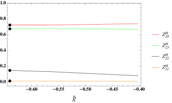
Figure 1: The Higgs mixing $Z^{H}_{2i}~{}(i=1,\ldots,4$) versus the gauge kinetic mixing coupling $\tilde{g}$. The values corresponding to the Benchmark Point (BP) of (forthcoming) Table 2(a) are labeled by $\bullet$.

The heavy Higgs boson tree-level mass eigenvalues are given in terms of the lightest SM-like Higgs boson $h\equiv{h_{1}}$ mass, which is fixed at $m_{h}=125~{}\text{GeV}$, and the lightest $B-L$ Higgs boson $h^{\prime}\equiv{h_{2}}$ mass, which we take to be $m_{h^{\prime}}=400~{}\text{GeV}$, as follows

$$m_{H,H^{\prime}}^{2}=\frac{1}{2}\left[~{}T_{H}-m_{h}^{2}-m_{h^{\prime}}^{2}\pm\sqrt{(T_{H}-m_{h}^{2}-m_{h^{\prime}}^{2})^{2}-\frac{4D_{H}}{m_{h}^{2}m_{h^{\prime}}^{2}}}~{}\right],$$ (12)

where we have the determinant $D_{H}=\text{Det}(M_{H}^{2})$ and the trace $T_{H}=\text{Tr}(M_{H}^{2})$ is given by

$$T_{H}=2|\mu|^{2}+m_{d}^{2}+m_{u}^{2}+2g^{2}v^{2}+2|\mu^{\prime}|^{2}+m_{2}^{2}+m_{1}^{2}+8g_{BL}^{2}x^{2}.$$ (13)

For $\sigma_{i}=\sigma_{d},\sigma_{u},\sigma_{1},\sigma_{2}$, one has $\sigma_{i}=Z^{H}_{ji}h_{j},~{}h_{j}=h,h^{\prime},H,H^{\prime}$ and $h_{j}=Z^{H}_{ij}\sigma_{i}$.

$$h^{\prime} \approx Z^{H}_{22}\sigma_{d}+Z^{H}_{23}\sigma_{1}+Z^{H}_{24}\sigma_{2}.$$ (14)

In Fig. 1, we display the mixing $Z^{H}_{2i}$ versus the gauge kinetic mixing $\tilde{g}$. As can be seen from this plot, $h^{\prime}$ is essentially generated from $\sigma_{1,2}$ with smaller contributions from the real components of $\sigma_{d}$ which connects it however to the SM sector. Table 2(a) presents the $B-L$ gaugino soft mass, $M_{\tilde{B}^{\prime}}$, and the MSSM and $B-L$ gaugino mixing soft mass, $M_{\tilde{B}\tilde{B}^{\prime}}$. The MSSM gaugino soft masses (bino, wino, gluino), $M_{\tilde{B}},M_{\tilde{W}},M_{\tilde{g}}$, are fixed to $M_{\tilde{B^{\prime}}}=M_{1}\sim 7.74\times 10^{2}~{}{\rm GeV}$, $M_{\tilde{W}}=M_{2}\sim 8.52\times 10^{2}~{}\text{GeV}$ and $M_{\tilde{g}}=M_{3}\sim 6.38\times 10^{2}~{}\text{GeV}$, respectively.

$g_{BL}$	$\tilde{g}$	$t_{\beta}$	$t_{\beta^{\prime}}$	$v^{\prime}$	$m_{u}^{2}$	$m_{d}^{2}$	$m_{1}^{2}$	$m_{2}^{2}$	$M_{\tilde{B}^{\prime}}$	$M_{\tilde{B}\tilde{B}^{\prime}}$
$0.675$	$-0.640$	$11.034$	$1.288$	$4875$	$-1.30\times 10^{7}$	$9.30\times 10^{6}$	$-5.75\times 10^{5}$	$4.02\times 10^{6}$	$1.49\times 10^{3}$	$-1.55\times 10^{3}$

(a) Our BP, wherein dimensionful parameters are all in GeV.

$Z^{H}_{11}$	$Z^{H}_{12}$	$Z^{H}_{13}$	$Z^{H}_{14}$	$Z^{H}_{21}$	$Z^{H}_{22}$	$Z^{H}_{23}$	$Z^{H}_{24}$	$Z^{H}_{31}$	$Z^{H}_{32}$	$Z^{H}_{33}$	$Z^{H}_{34}$	$Z^{H}_{41}$	$Z^{H}_{42}$	$Z^{H}_{43}$	$Z^{H}_{44}$
$0.089$	$0.987$	$-0.100$	$-0.088$	$0.012$	$0.131$	$0.678$	$0.723$	$0.030$	$0.009$	$0.728$	$-0.685$	$-0.995$	$0.091$	$0.021$	$-0.019$

(b) Neutral CP-even Higgs mixing corresponding to the BP of Table 2(a).

$m_{H^{\pm}}$	$m_{A}$	$m_{A^{\prime}}$	$m_{h_{1}\equiv h}$	$m_{h_{2}\equiv h^{\prime}}$	$m_{h_{3}\equiv H^{\prime}}$	$m_{h_{4}\equiv H}$	$M_{Z^{\prime}}$
$4384$	$2587$	$4384$	$125$	$397$	$4241$	$4402$	$3300$

(c) Higgs mass spectrum and $M_{Z^{\prime}}$ in GeV corresponding to the BP of Table 2(a).

The Higgs bosons interaction couplings with fermion and gauge bosons are

$$\Gamma^{h_{2}}_{\bar{d}d} =-\frac{1}{\sqrt{2}}Y^{d}Z^{H}_{22}=-\frac{m_{d}}{vc_{\beta}}Z^{H}_{22},$$ (15)

$$\Gamma^{h_{2}}_{\bar{u}u} =-\frac{1}{\sqrt{2}}Y^{u}Z^{H}_{22}=-\frac{m_{u}}{vs_{\beta}}Z^{H}_{22},$$ (16)

$$g_{h^{\prime}W^{+}W^{-}} \approx g_{2}M_{W}s_{\beta}Z^{H}_{22},$$ (17)

$$g_{h^{\prime}ZZ} \approx g_{h^{\prime}W^{+}W^{-}}\left(\sec\theta_{w}-\frac{\tilde{g}}{g_{2}}s_{\theta_{w^{\prime}}}\right)^{2},$$ (18)

$$g_{h^{\prime}hh} \approx\frac{1}{4}Z_{{22}}^{H}\Big{(}4\tilde{g}g_{BL}xZ_{{12}}^{H}\Big{(}Z_{{13}}^{H}s_{\beta^{\prime}}-Z_{{14}}^{H}c_{\beta^{\prime}}\Big{)}-3g^{2}vs_{\beta}(Z_{{12}}^{H})^{2}\Big{)}$$

$$+\frac{1}{2}Z_{{23}}^{H}\Big{(}2g_{BL}^{2}x\Big{(}3s_{\beta^{\prime}}(Z_{{13}}^{H})^{2}-2c_{\beta^{\prime}}Z_{{13}}^{H}Z_{{14}}^{H}-s_{\beta^{\prime}}(Z_{{14}}^{H})^{2}\Big{)}-\tilde{g}g_{BL}\Big{(}xs_{\beta^{\prime}}(Z_{{12}}^{H})^{2}+2vs_{\beta}Z_{{12}}^{H}Z_{{13}}^{H}\Big{)}\Big{)}$$

$$+\frac{1}{2}Z_{{24}}^{H}\Big{(}2g_{BL}^{2}x\Big{(}c_{\beta^{\prime}}(Z_{{13}}^{H})^{2}+2s_{\beta^{\prime}}Z_{{13}}^{H}Z_{{14}}^{H}-3c_{\beta^{\prime}}(Z_{{14}}^{H})^{2}\Big{)}\Big{)},$$ (19)

where $\theta_{w}$ and $\theta_{w^{\prime}}$ are the weak and $Z-Z^{\prime}$ mixing angles, respectively. For $t_{\beta^{\prime}}\sim 1$, $Z_{{12}}^{H}\sim 1,~{}Z_{{13}}^{H},Z_{{14}}^{H}\ll 1,~{}Z_{{23}}^{H},Z_{{24}}^{H}\sim\frac{1}{\sqrt{2}}$, the trilinear Higgs boson coupling $h^{\prime}hh$ (relevant to our forthcoming analysis) is approximated by

$$g_{h^{\prime}hh} \approx-\frac{1}{2}(Z_{{12}}^{H})^{2}\Big{(}\frac{3}{2}g^{2}vs_{\beta}Z_{{22}}^{H}+\tilde{g}g_{BL}x\big{(}s_{\beta^{\prime}}Z_{{23}}^{H}+c_{\beta^{\prime}}Z_{{24}}^{H}\big{)}\Big{)}$$

$$\sim-\frac{1}{2}\Big{(}\frac{3}{2}g^{2}vs_{\beta}Z_{{22}}^{H}+\frac{1}{\sqrt{2}}\tilde{g}g_{BL}x\big{(}s_{\beta^{\prime}}+c_{\beta^{\prime}}\big{)}\Big{)}$$

$$\sim-\frac{1}{2}\Big{(}\frac{3}{2}g^{2}vs_{\beta}Z_{{22}}^{H}+\tilde{g}g_{BL}x\Big{)}.$$ (20)

We notice, from Eq. (20), that setting the gauge kinetic mixing coupling $\tilde{g}\equiv 0$ reduces the $g_{h^{\prime}hh}$ coupling.

III SEARCH FOR A HEAVY Neutral CP-EVEN Higgs BOSON AT THE LHC

Many computational tools are used throughout this work, from building the model analytically to performing the numerical simulations at detector level. The BLSSM was first implemented into the Sarah package for Mathematica and the output was then passed to SPheno [23, 24] for numerical calculations of the particle spectrum. After that, the ensuing UFO model was used in MadGraph [25] for MC event generation and Matrix Element (ME) calculations. After that, Pythia was used to simulate initial and final state radiation (through the Parton Shower (PS) formalism) as well as fragmentation/hadronization effects [26]. For detector simulation, the Pythia output was passed to Delphes [27]. Finally, for data analysis, we used MadAnalysis [28]. As for the BP used, we made sure that it was consistent with HiggsBounds and HiggsSignals [29, 30] limits, as obtained from the latest LHC data.

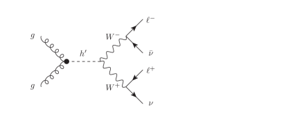
Figure 2: Feynman diagrams for $h^{\prime}$ production via ggF and decays via (from left to right) $W^{+}W^{-}\to 2\ell+\not{E}_{T}$, $h^{\prime}\to ZZ\to 4\ell$ and $h^{\prime}\to{hh}\to{b\bar{b}\gamma\gamma}$.

The Feynman diagrams associated to the $h^{\prime}$ production and decay mechanisms discussed here are found in Fig. 2, wherein the $\bullet$ symbol is meant to signify the exact loop function allowing for both $b$ and $t$ quark contributions. The Higgs production and decay rates of are computed by factorising the $h^{\prime}$ propagator, so that the overall event yield can be broken down into the $h^{\prime}$ production cross section and decay Branching Ratios (BRs). The MC event generation is done at Leading Order (LO) for both Signal ($S$) and Background ($B$), however, we include Next-to-Next-to-LO (NNLO) inclusive $k$-factors from Quantum Chromo-Dynamics (QCD) in computing our significances, specifically, we use 2.2 for the ggF signal and 1.2 for the Vector Boson Fusion (VBF) one (see below) as well as the (EW) backgrounds [31, 32, 33, 34, 35].

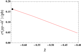
Figure 3: ggF $h^{\prime}$ production cross section at $\sqrt{s}=14~{}\text{TeV}$ (left) and $h^{\prime}$ decay BRs (right) versus the kinetic mixing coupling $\tilde{g}$. The values corresponding to the BP of Table 2(a) are labeled by $\bullet$.

The cross section for ggF, properly convoluted with the default Parton Distribution Functions (PDFs) of our ME generator (namely, $\sigma(pp\to h^{\prime})$), as function of $\tilde{g}$, is found in Fig. 3 (left), for $\sqrt{s}=14$ TeV. In Fig. 3 (right) we show instead the $h^{\prime}$ decay BRs, again, as functions of $\tilde{g}$. In both such plots, the symbol $\bullet$ refers to the BP adopted here, for which the corresponding $\sigma$ and BR values are found in Table 3. The production cross section of $h^{\prime}$ depends significantly on $\tilde{g}$, which is (as mentioned) the only source of mixing between the BLSSM Higgs $\chi_{1,2}$ and the MSSM Higgs doublets $H_{u,d}$ that enables $h^{\prime}$ couplings with SM particles. However, the $h^{\prime}$ decay BRs are not significantly affected by it because both the partial and total decay widths of $h^{\prime}$ in each channel receive nearly the same contribution from $\tilde{g}$, which cancels out from the BRs. It is noteworthy that the three most significant decay channels are the bosonic ones in $W^{+}W^{-}$, $ZZ$ and $hh$. In contrast, the fermionic decay channels into $t\bar{t}$ and $b\bar{b}$ are relatively less significant. Therefore, in the forthcoming MC analysis, we will concentrate on the former three decay channels.

For each channel, there are many corresponding background processes and all can be reduced by applying the cut-flows of Tables  4(a), 4(b) and 4(c), in correspondence of the three aforementioned channels, respectively. What remain in all cases, though, are the irreducible backgrounds $pp\to{2\ell}+\not{E}_{T}$, $pp\to{4\ell}$ and $pp\to{\gamma\gamma{b\bar{b}}}$.

The following standard acceptance cuts on transverse momentum $(P_{T})$, pseudorapidity $(\eta)$ and angular separation $(\Delta{R})$ of the final state leptons, jets and photons are applied:

1. $(P_{T})_{j}\geq 20,~{}(P_{T})_{a}\geq 10,~{}a=\gamma,\ell$,

2. $|\eta_{j}|\leq 5,~{}|\eta_{a}|\leq 2.5,~{}a=\gamma,\ell$,

3. $\Delta{R}_{ab}\geq 0.4,~{}a,b=j,\gamma,\ell$.

In Tables  4(a), 4(b) and 4(c), the kinematical variables are defined such that $M_{\text{eff}}$ is the effective mass being obtained as the sum of the transverse momentum of all final state objects and the transverse energy, and $E_{T}$ is the scalar sum of the transverse energy of all (visible) final state objects in the plane transverse to the beam [28]. Furthermore, $M_{ab\ldots}$ is an invariant mass and $\Delta{R}_{ab}$ is the separation between final state objects. (Note that an (opposite-sign) di-lepton mass reconstruction around one $M_{Z}$ value in the $4\ell$ channel is not useful, as the irreducible background is here dominated by $pp\to ZZ,Z\gamma^{*}\to 4\ell$.)

Quantity	Value
$\text{BR}(h^{\prime}\to W^{+}W^{-})$	$0.432$
$\text{BR}(h^{\prime}\to ZZ)$	$0.203$
$\text{BR}(h^{\prime}\to{hh})$	$0.261$
$\sigma(pp\to h^{\prime})$	$163.400~{}\text{(fb)}$
$\sigma(pp\to h^{\prime}\to W^{+}W^{-}\to 2\ell+\not{E}_{T})$	$~{}~{}9.256~{}\text{(fb)}$
$\sigma(pp\to h^{\prime}\to ZZ\to 4\ell)$	$~{}~{}0.406~{}\text{(fb)}$
$\sigma(pp\to h^{\prime}\to{hh}\to\bar{b}b\gamma\gamma)$	$~{}~{}0.124~{}\text{(fb)}$

Table 3: Production cross section $\sigma$ (at $\sqrt{s}=14~{}\text{TeV}$) and decay BRs into $W^{+}W^{-}$, $ZZ$ and $hh$ for the $h^{\prime}$ state (with $m_{h^{\prime}}=400~{}\text{GeV}$) of our BP, including the overall rates in the three final states $2\ell+\not{E}_{T}$, $4\ell$ and $b\bar{b}\gamma\gamma$. Normalization is to LO for all $\sigma$’s.

Cuts (select)	$S$	$B$	$S/\sqrt{B}$
Initial (no cut)	$6108$	$720000$	$7.20$
$E_{T}>700~{}\text{GeV}$	$703.1\pm 24.9$	$2219.9\pm 47.0$	$14.92\pm 0.008$
$M_{\text{eff}}>100~{}\text{GeV}$	$693.1\pm 24.8$	$2118.5\pm 46.2$	$15.06\pm 0.008$
$\Delta R_{\ell^{+}\ell^{-}}>1.5$	$628.2\pm 23.7$	$1568.3\pm 39.6$	$15.86\pm 0.009$

(a) $pp\to h^{\prime}\to W^{+}W^{-}\to 2\ell+\not{E}_{T}$ cut-flow at $L_{\text{int}}=300~{}\text{fb}^{-1}$.

Cuts (select)	$S$	$B$	$S/\sqrt{B}$
Initial (no cut)	$267$	$9712$	$2.72$
$E_{T}>300~{}\text{GeV}$	$208.75\pm 6.79$	$1680.2\pm 37.30$	$5.09\pm 0.004$
$M_{\ell^{+}\ell^{-}}<150~{}\text{GeV}$	$173.04\pm 7.83$	$1414.9\pm 34.80$	$4.60\pm 0.005$
$M_{\ell^{+}\ell^{-}}>50~{}\text{GeV}$	$172.80\pm 7.83$	$1394.7\pm 34.60$	$4.63\pm 0.005$

(b) $pp\to h^{\prime}\to{ZZ}\to 4\ell$ cut-flow at $L_{\text{int}}=300~{}\text{fb}^{-1}$.

Cuts (select)	$S$	$B$	$S/\sqrt{B}$
Initial (no cut)	$951$	$19951560$	$0.213$
$E_{T}>200~{}\text{GeV}$	$933.18\pm 4.19$	$1476867.0\pm 1169.0$	$0.768\pm 2.88\times 10^{-6}$
$M_{\gamma\gamma}>120~{}\text{GeV}$	$475.50\pm 15.40$	$165131.0\pm 404.0$	$1.170\pm 9.31\times 10^{-5}$
$M_{\gamma\gamma}<135~{}\text{GeV}$	$474.80\pm 15.40$	$29023.0\pm 170.0$	$2.787\pm 5.23\times 10^{-4}$
$M_{bb}>50~{}\text{GeV}$	$145.50\pm 11.10$	$3582.7\pm 59.9$	$2.431\pm 2.93\times 10^{-3}$
$M_{bb}<160~{}\text{GeV}$	$134.70\pm 10.80$	$1944.9\pm 44.1$	$3.055\pm 5.03\times 10^{-3}$
$\Delta R_{\gamma\gamma}<3.5$	$133.90\pm 10.7$	$1824.5\pm 42.7$	$3.135\pm 5.32\times 10^{-3}$
$\Delta R_{b\bar{b}}<3.5$	$131.90\pm 10.7$	$1746.2\pm 41.8$	$3.156\pm 5.50\times 10^{-3}$
$M_{\gamma\gamma\bar{b}b}>360~{}\text{GeV}$	$102.71\pm 9.57$	$686.4\pm 26.2$	$3.920\pm 1.14\times 10^{-2}$
$M_{\gamma\gamma\bar{b}b}<450~{}\text{GeV}$	$98.5\pm 9.40$	$403.4\pm 20.1$	$4.903\pm 1.70\times 10^{-2}$

(c) $pp\to h^{\prime}\to{hh}\to{b\bar{b}\gamma\gamma}$ cut-flow at $L_{\text{int}}=3000~{}\text{fb}^{-1}$.

Table 4: $S$ vs $B$ rates for the three signals pursued in our analysis in correspondence of our BP: the $2\ell+\not{E}_{T}$ (a), $4\ell$ and $b\bar{b}\gamma\gamma$ (c) final state. We adopt here $\sqrt{s}=14~{}\text{TeV}$ and integrated luminosity of Run 3 and HL-LHC. Inclusive NNLO $k$-factors from QCD are used here throughout.

III.1 THE $h^{\prime}\to W^{+}W^{-}\to 2\ell+\not{E}_{T}$ CHANNEL

Table 4(a) provides the cut-flow for the $h^{\prime}$ production and decay analysis via the $2\ell+\not{E}_{T}$ signature, while event shapes and rates (the latter in correspondence to Run 3 luminosity) for

$$\sigma(pp\to h^{\prime}\to W^{+}W^{-}\to 2\ell+\not{E}_{T})\approx\sigma(pp\to h^{\prime})\times\text{BR}(h^{\prime}\to W^{+}W^{-}\to 2\ell+\not{E}_{T})$$ (21)

are presented in Fig. 4. Herein, we also present the contributions of an additional signal channel, induced by ($W^{+}W^{-}$ dominated) VBF with two additional (untagged) forward/backward jets, as it contributes not negligibly to the same ggF signal regions (so that it has been taken into account in extracting our final sensitivities). In this figure, the normalized (to 1) distributions used for the cut-flow (i.e., $E_{T}$, $M_{\rm eff}$ and $\Delta R_{\ell^{+}\ell^{-}}$) are presented, alongside the full transverse mass ($M_{T_{\ell^{+}\ell^{-}}}$) of the final state (i.e., using both leptons in its definition), the latter integrating to the actual event numbers for Run 3 and also in presence of the background contribution. Altogether, from this last spectrum, it is clear that a high signal significance can be reached, however, it also shows that the shape does not promptly correlate to the $h^{\prime}$ mass value. Yet, the significant excess seen in this channel will clearly motivate a parallel search in the $4\ell$ final state, which we are illustrating next.

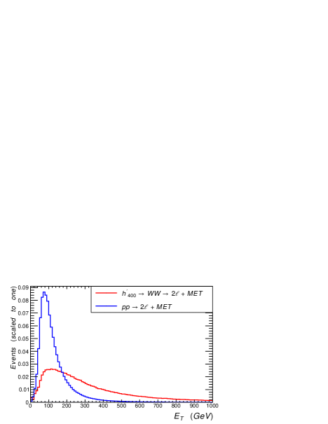
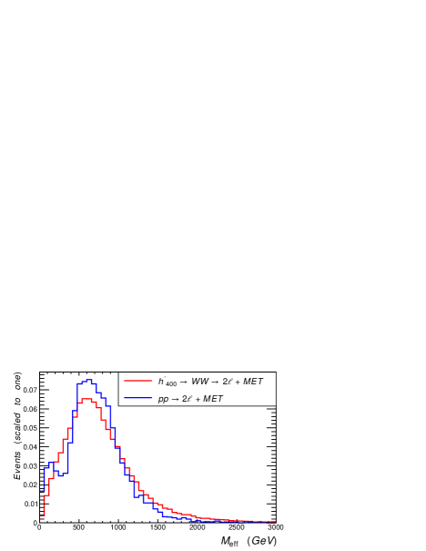
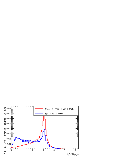
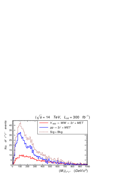
Figure 4: $S$ and $B$ distributions in $E_{T}$ (top-left), $M_{\rm eff}$ (top-right), $\Delta R_{\ell^{+}\ell^{-}}$ (bottom-left) and $M_{T_{\ell^{+}\ell^{-}}}$ (bottom-right), as defined in the text, the former three given before the cut-flow and normalized to 1 while the latter one given after it and normalized to the total event rate for the integrated luminosity $L_{\text{int}}=300~{}\text{fb}^{-1}$. In all cases we show both the ggF contribution to the signal $2\ell+\not{E}_{T}$ (red) for our BP and the background (blue) while for the last spectrum we also show the (stacked) distribution as well.

III.2 THE $h^{\prime}\to{ZZ}\to 4\ell$ CHANNEL

Table 4(b) provides the cut-flow for $h^{\prime}$ production and decay via the $4\ell$ channel, while some relevant kinematics, in terms of event shapes and rates (the latter, again, in correspondence to Run 3 luminosity) for

$$\sigma(pp\to h^{\prime}\to ZZ\to 4\ell)\approx\sigma(pp\to h^{\prime})\times\text{BR}(h^{\prime}\to ZZ\to 4\ell)$$ (22)

is presented in Fig. 5. Here, we concentrate on the normalized (to 1) distributions in transverse energy of all leptons ($E_{T}$) and opposite-sign di-lepton invariant mass ($M_{\ell^{+}\ell^{-}}$), both of which are used in our cut-flow. (Regarding the latter, notice that the loss of significance in applying the cut in invariant mass against the dominant irreducible background $pp\to ZZ,Z\gamma^{*}\to 4\ell$ is rather insignificant against the benefits of rejecting the irreducible one, e.g., from top-antitop quark production and fully leptonic $W^{+}W^{-}$ decays (which has typically a harder distribution in this variable), so that the whole of the latter can be neglected.) In the end, the spectrum from which to extract the $h^{\prime}$ resonance, i.e., the final state invariant mass, $M_{4\ell}$, clearly reveals a broad excess over a 400 GeV or so mass interval, altogether yielding significances in the discovery range. In fact, also a noticeable peak appear for $M_{4\ell}\approx 400$ GeV (which, as mentioned, can be correlated with the $M_{T_{\ell^{+}\ell^{-}}}$ distribution in the $2\ell+\not{E}_{T}$ final state), so that one can improve further the potential for $h^{\prime}$ discovery in the $4\ell$ channel by optimizing a cut in this variable.

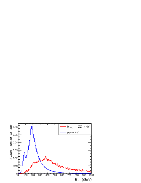
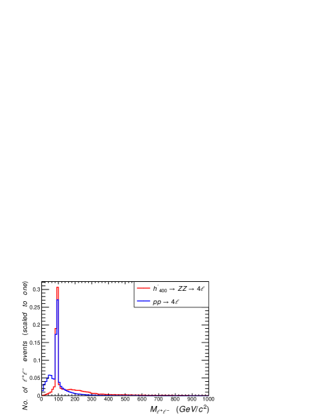
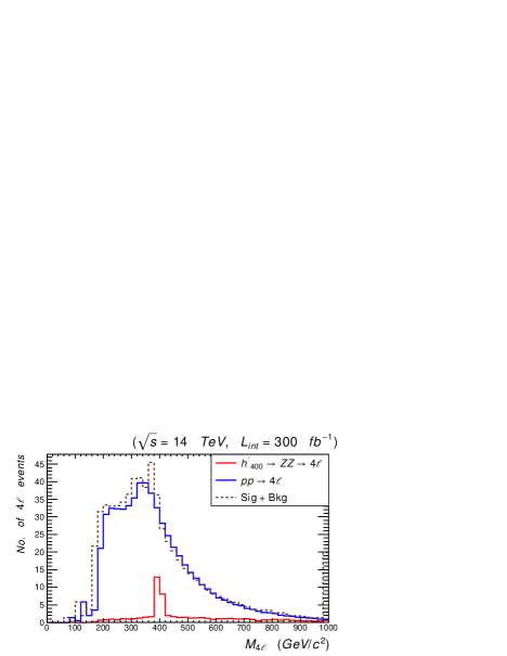
Figure 5: $S$ and $B$ distributions in $E_{T}$ (top-left), $M_{\ell^{+}\ell^{-}}$ (top-right) and $M_{4\ell}$ (bottom), as defined in the text, the former two given before the cut-flow and normalized to 1 while the latter one given after it and normalized to the total event rate for the integrated luminosity $L_{\text{int}}=300~{}\text{fb}^{-1}$. In all cases we show only the ggF contribution to the $4\ell$ signal for our BP while for the last spectrum we also show the (stacked) distribution.

III.3 THE $h^{\prime}\to{hh}\to{b\bar{b}\gamma\gamma}$ CHANNEL

Table 4(c) provides the cut-flow for the $h^{\prime}$ production and decay analysis of the last channel we study,

$$\sigma(pp\to h^{\prime}\to{hh}\to{b\bar{b}\gamma\gamma})\approx\sigma(pp\to h^{\prime})\times\text{BR}(h^{\prime}\to{hh}\to{b\bar{b}\gamma\gamma}),$$ (23)

wherein we use HL-LHC luminosity, as this channel is not accessible during Run 3. The distributions used to inform our cut-flow herein (normalized to 1) are found in Fig. 6. These are the spectra in the transverse energy of the $b\bar{b}\gamma\gamma$ final state ($E_{T}$), $\gamma\gamma$ and $b\bar{b}$ invariant masses ($M_{\gamma\gamma}$ and $M_{b\bar{b}}$, respectively) and separations ($\Delta R_{\gamma\gamma}$ and $\Delta R_{b\bar{b}}$, respectively). Such a figure also presents the invariant mass of the final state ($M_{\gamma\gamma b\bar{b}}$), normalized to the HL-LHC luminosity. As seen from the signal and background responses to the cut-flow, it is clear that knowledge of the $m_{h^{\prime}}$ value, gained during Run 3 of the LHC by exploiting the two previous signatures, is crucial in accessing this signal, which can ultimately be done at the 5$\sigma$ level, despite the initially overwhelming background.

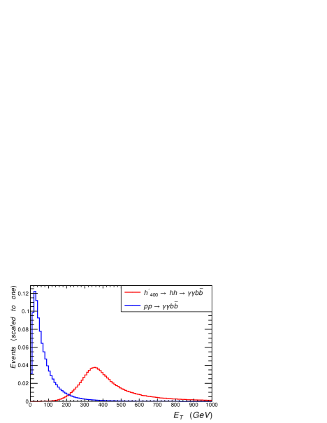
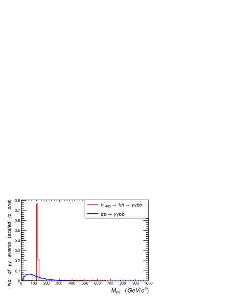
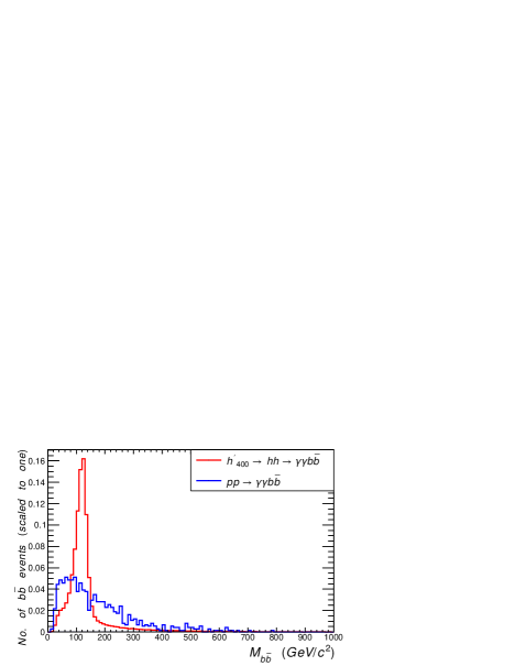
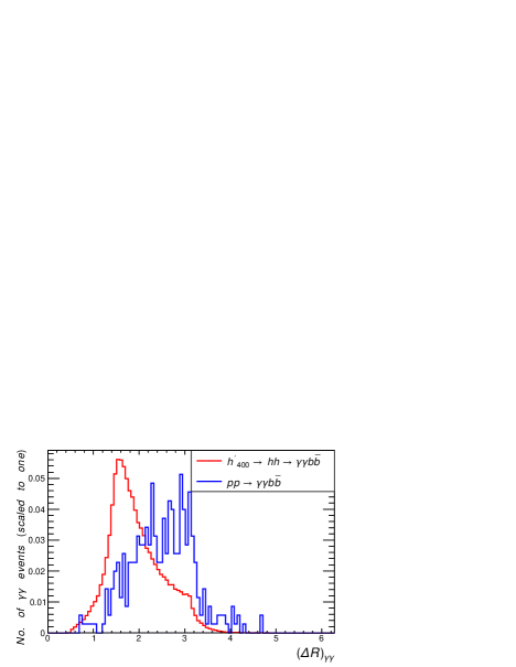
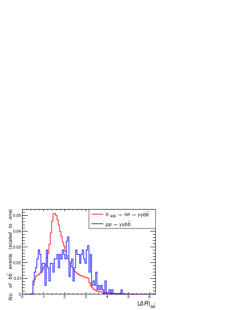
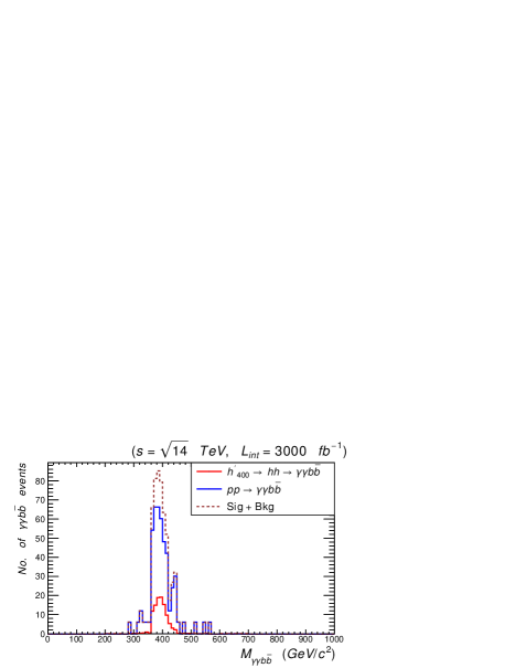
Figure 6: $S$ and $B$ distributions in $E_{T}$ (top-left), $M_{\gamma\gamma}$ (top-right), $M_{b\bar{b}}$ (middle-left), $\Delta R_{\gamma\gamma}$ (middle-right) $\Delta R_{b\bar{b}}$ (bottom-left) and $M_{\gamma\gamma b\bar{b}}$ (bottom-right), as defined in the text, the former 5 given before the cut-flow and normalized to 1 while the latter one given after it and normalized to the total event rate for the integrated luminosity $L_{\text{int}}=3000~{}\text{fb}^{-1}$. In all cases we show only the ggF contribution to the $b\bar{b}\gamma\gamma$ signal for our BP while for the last spectrum we also show the (stacked) distribution.

III.4 Historical Significances

Before closing this section, we describe the patterns of significances in the three channels that we have studied, as they would evolve with luminosity, assuming fixed energy at $\sqrt{s}=14$ TeV. These are shown in Fig. 7. lt is evident that a full characterization of the $h^{\prime}$ state, involving its coupling to SM (massive) gauge and Higgs bosons is only possible through a combined effort of analyses to be entertained at both Run 3 of the LHC and HL-LHC.

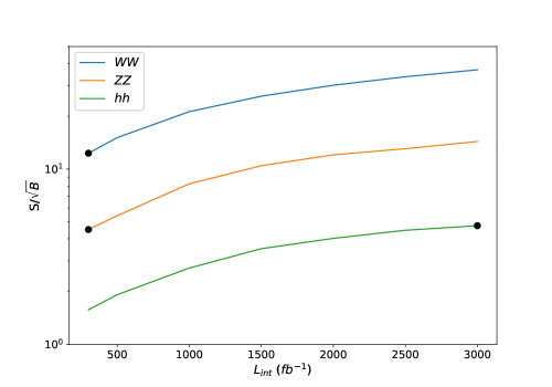
Figure 7: Significance of the $h^{\prime}\to W^{+}W^{-},ZZ$ and $hh$ signals that we have studied versus $L_{\text{int}}$ for our BP. Data are produced at a center-of-mass energy of $\sqrt{s}=14~{}\text{TeV}$. The rates are computed after applying the relevant kinematical analyses described in the text. The three $\bullet$ points indicate the luminosity choices used in the MC simulations performed.

IV CONCLUSIONS

In summary, we have shown that a theoretically well-motivated realization of supersymmetry, the so-called BLSSM, may yield detectable signals of a heavy neutral CP-even Higgs boson at the LHC, both during Run 3 and the HL-LHC phase. These emerge from the lightest (neutral) Higgs state of this scenario with prevalent $B-L$ composition, $h^{\prime}$, while the lightest (neutral) Higgs state with predominant MSSM nature is identified with the discovered one, $h$ (with $m_{h}=125~{}\text{GeV}$). The subprocesses pursued to this effect, assuming a BP with an illustrative mass $m_{h^{\prime}}=400~{}\text{GeV}$, have been $gg\to h^{\prime}\to W^{+}W^{-}\to 2\ell+\not{E}_{T}$, $gg\to h^{\prime}\to{ZZ}\to 4\ell$ and $gg\to h^{\prime}\to{hh}\to{b\bar{b}\gamma\gamma}$. The first one would be accessible during the early stages of Run 3 and the study of mass distributions would allow one to extract an indication of the $h^{\prime}$ mass. This information can then be used to optimize the selection of the second signal, which would reveal a clear pick centered around $m_{h^{\prime}}$ by the end of Run 3. With the latter information available, one would then be able to establish the third signal at the HL-LHC. All this will therefore enable one to fully characterize the $h^{\prime}$ state, not only through its mass, but also in terms of its couplings, as the $W^{+}W^{-}$, $ZZ$ and $hh$ decays are the dominant ones in the BLSSM while those to $t\bar{t}$ and $b\bar{b}$ pairs may be accessible at production level through the ggF channel. This finally opens up the possibility of eventually separating the BLSSM hypothesis from alternative ones also based on supersymmetry, since – thanks to the peculiar feature of (gauge) kinetic mixing appearing in the BLSSM (which incorporates an additional $U(1)_{B-L}$ group beyond the SM gauge symmetries) – competing signals stemming from, e.g., the MSSM would have rather different mass and coupling patterns.

We have come to these conclusions by performing a full MC analysis in presence of ME, PS, fragmentation/hadronization effects as well as detector modeling and upon devising dedicated cut-and-count cut-flows for each signature pursued. We are therefore confident that ATLAS and CMS would have sensitivity to this specific non-minimal realization of supersymmetry and advocate dedicate searches for the aforementioned signals.

References

- ATLAS-Collaboration [2022a] ATLAS-Collaboration (ATLAS) (2022a), eprint 2211.02617.
- ATLAS-Collaboration [2022b] ATLAS-Collaboration (ATLAS) (2022b), eprint 2211.01136.
- CMS-Collaboration [2022] CMS-Collaboration (CMS) (2022), eprint 2210.00043.
- Adhikary et al. [2021] A. Adhikary, B. Bhattacherjee, R. M. Godbole, N. Khan, and S. Kulkarni, JHEP 04, 284 (2021), eprint 2002.07137.
- Chen et al. [2020] X. Chen, Y. Xu, Y. Wu, Y.-P. Kuang, Q. Wang, H. Chen, S.-C. Hsu, Z. Hu, and C. Li, Phys. Lett. B 804, 135358 (2020), eprint 1905.05421.
- Bahl et al. [2020] H. Bahl, P. Bechtle, S. Heinemeyer, S. Liebler, T. Stefaniak, and G. Weiglein, Eur. Phys. J. C 80, 916 (2020), eprint 2005.14536.
- Gu et al. [2017] J. Gu, H. Li, Z. Liu, S. Su, and W. Su, JHEP 12, 153 (2017), eprint 1709.06103.
- Banerjee et al. [2015] S. Banerjee, M. Mitra, and M. Spannowsky, Phys. Rev. D 92, 055013 (2015), eprint 1506.06415.
- Hammad et al. [2016] A. Hammad, S. Khalil, and S. Moretti, Phys. Rev. D 93, 115035 (2016), eprint 1601.07934.
- Aad et al. [2012] G. Aad et al. (ATLAS), Phys. Lett. B 716, 1 (2012), eprint 1207.7214.
- Chatrchyan et al. [2012] S. Chatrchyan et al. (CMS), Phys. Lett. B 716, 30 (2012), eprint 1207.7235.
- Chernyavskaya [2023] N. Chernyavskaya, in 55th Rencontres de Moriond on Electroweak Interactions and Unified Theories (2023), eprint 2302.12631.
- Djouadi [2008] A. Djouadi, Phys. Rept. 459, 1 (2008), eprint hep-ph/0503173.
- Moretti and Khalil [2019] S. Moretti and S. Khalil, Supersymmetry Beyond Minimality: From Theory to Experiment (CRC Press, 2019), ISBN 978-0-367-87662-3.
- Hammad et al. [2015] A. Hammad, S. Khalil, and S. Moretti, Phys. Rev. D 92, 095008 (2015), eprint 1503.05408.
- Abdallah et al. [2015] W. Abdallah, S. Khalil, and S. Moretti, Phys. Rev. D 91, 014001 (2015), eprint 1409.7837.
- Abdelalim et al. [2022] A. A. Abdelalim, B. Das, S. Khalil, and S. Moretti, Nucl. Phys. B 985, 116013 (2022), eprint 2012.04952.
- Khalil and Masiero [2008] S. Khalil and A. Masiero, Phys. Lett. B 665, 374 (2008), eprint 0710.3525.
- O’Leary et al. [2012] B. O’Leary, W. Porod, and F. Staub, JHEP 05, 042 (2012), eprint 1112.4600.
- Basso [2011] L. Basso, Ph.D. thesis, Southampton U. (2011), eprint 1106.4462.
- Basso [2015] L. Basso, Adv. High Energy Phys. 2015, 980687 (2015), eprint 1504.05328.
- Khalil [2016] S. Khalil, Phys. Rev. D 94, 075003 (2016), eprint 1606.09292.
- Staub [2014] F. Staub, Comput. Phys. Commun. 185, 1773 (2014).
- Porod and Staub [2012] W. Porod and F. Staub, Comput. Phys. Commun. 183, 2458 (2012).
- Alwall et al. [2011] J. Alwall, M. Herquet, F. Maltoni, O. Mattelaer, and T. Stelzer, JHEP 06, 128 (2011).
- Sjostrand et al. [2008] T. Sjostrand, S. Mrenna, and P. Z. Skands, Comput. Phys. Commun. 178, 852 (2008).
- de Favereau et al. [2014] J. de Favereau, C. Delaere, P. Demin, A. Giammanco, V. Lemaître, A. Mertens, and M. Selvaggi (DELPHES 3), JHEP 02, 057 (2014).
- Conte et al. [2013] E. Conte, B. Fuks, and G. Serret, Comput. Phys. Commun. 184, 222 (2013).
- Bechtle et al. [2014a] P. Bechtle, O. Brein, S. Heinemeyer, O. Stål, T. Stefaniak, G. Weiglein, and K. E. Williams, Eur. Phys. J. C 74, 2693 (2014a).
- Bechtle et al. [2014b] P. Bechtle, S. Heinemeyer, O. Stål, T. Stefaniak, and G. Weiglein, Eur. Phys. J. C 74, 2711 (2014b).
- Harlander and Kilgore [2001] R. V. Harlander and W. B. Kilgore, eConf C010630, P506 (2001), eprint hep-ph/0110200.
- Harlander and Kilgore [2002] R. V. Harlander and W. B. Kilgore, Phys. Rev. Lett. 88, 201801 (2002), URL https://link.aps.org/doi/10.1103/PhysRevLett.88.201801.
- Ciccolini et al. [2008] M. Ciccolini, A. Denner, and S. Dittmaier, Phys. Rev. D 77, 013002 (2008), eprint 0710.4749.
- Baglio et al. [2019] J. Baglio, F. Campanario, S. Glaus, M. Mühlleitner, M. Spira, and J. Streicher, Eur. Phys. J. C 79, 459 (2019), eprint 1811.05692.
- Schmidt and Spira [2016] T. Schmidt and M. Spira, Phys. Rev. D 93, 014022 (2016), eprint 1509.00195.