RGCVAE: Relational Graph Conditioned Variational Autoencoder for Molecule Design

Abstract

Identifying molecules that exhibit some pre-specified properties is a difficult problem to solve. In the last few years, deep generative models have been used for molecule generation. Deep Graph Variational Autoencoders are among the most powerful machine learning tools with which it is possible to address this problem. However, existing methods struggle in capturing the true data distribution and tend to be computationally expensive.

In this work, we propose RGCVAE, an efficient and effective Graph Variational Autoencoder based on: (i) an encoding network exploiting a new powerful Relational Graph Isomorphism Network; (ii) a novel probabilistic decoding component. Compared to several state-of-the-art VAE methods on two widely adopted datasets, RGCVAE shows state-of-the-art molecule generation performance while being significantly faster to train.

1 Introduction

Chemical space is huge, and it contains many (unknown) molecules which can turn useful in many industrial and pharmaceutical areas, e.g. to develop new improved drugs. The problem is how to search such space in an efficient and targeted way. Traditional approaches, such as high throughput screening Curtarolo et al. (2013); Pyzer-Knapp et al. (2015), combinatorial and evolutionary algorithms Devi et al. (2015), are substantially based on brute force search, possibly improved using heuristics. More recent approaches are based on availability of data (e.g., a corpus of molecules with known properties) to which Machine Learning approaches are applied. For example, Recursive Neural Networks or graph kernels have been used to predict properties of pre-defined or commercial compounds Bianucci et al. (2003); Bernazzani et al. (2006), and Generative Models have been used to generate candidate molecules that are likely to exhibit some pre-specified properties Blaschke et al. (2018); Oglic et al. (2018).

Generation of candidate molecules seems to be a quite promising approach since, based on a family of compounds for which the property of interest is known, the model should be able to capture the common features that deliver the property of interest. If this is the case, the generation process is also required to produce molecules which are novel and useful.

Models for the generation of new molecules mainly represent the molecule structures as: (i) SMILES strings that describe the molecule structures, such as in Weininger (1988); Weininger et al. (1989); Weininger (1990); (ii) graph representations, in which nodes represent atoms and edges represent bonds, such as in Rigoni et al. (2020a); Liu et al. (2018); Ma et al. (2018); (iii) graph representations, in which nodes represents molecules’ substructures, such as in Jin et al. (2018, 2020). Since it is simpler to deal with strings than graphs, early works adopted the SMILES representation, while more recent works use the graph representation because of its greater expressiveness. Both the SMILES representation and the graph representation of molecules have advantages and disadvantages. For example, graph representations are more expressive than the SMILES representations, but in contrast, are harder to learn.

Several early works are based on the Variational Autoencoder (VAE) Kingma and Welling (2014) approach, such as Character VAE Gómez-Bombarelli et al. (2018) which uses a variational autoencoder to directly predict the molecule SMILES representation, Grammar VAE Kusner et al. (2017) which adds a context-free grammar to Character VAE to guide the correct generation of SMILES strings, and Syntax Directed VAE Dai et al. (2018) which adds a more expressive grammar, the attribute grammar Knuth (1968), capable of generating a higher number of valid SMILES strings. The VAE approach has also been used by models which consider the graph representation of the molecules, e.g. Junction Tree VAE Jin et al. (2018), Regularized Graph VAE Ma et al. (2018), Constrained Graph VAE (CGVAE) Liu et al. (2018), and Conditional CGVAE Rigoni et al. (2020a).

Other works are based on recurrent neural networks Segler et al. (2018); Podda et al. (2020), adversarial autoencoders Makhzani et al. (2015); Kadurin et al. (2017); Polykovskiy et al. (2018), generative adversarial networks Arjovsky et al. (2017); Guimaraes et al. (2017) and Flow based models Shi et al. (2020); Zang and Wang (2020); Kuznetsov and Polykovskiy (2021). More recently, some works address the generation of new molecules starting from a set of reactants that need to be combined together to form a new molecule Bradshaw et al. (2019, 2020). To evaluate and compare this variety of models, a systematic model comparison Rigoni et al. (2020b) and some frameworks have been developed, such as MOSES Polykovskiy et al. (2018) and GuacaMol Brown et al. (2019).

Some of these models, in addition to generating new molecules, allow to optimize a given molecule structure towards those that exhibit a better pre-specified property using: (i) an ad-hoc optimization process  Gómez-Bombarelli et al. (2018); Kusner et al. (2017); Dai et al. (2018); Jin et al. (2018); Liu et al. (2018), or (ii) introducing additional terms in the loss function De Cao and Kipf (2018); Ma et al. (2018).

However, in this work we mainly focus on the distribution learning task, which is defined as the task of learning the probability distribution that has generated the molecules in the dataset, instead of the structure optimization task that aims to optimize a given molecule structure to exhibit a better pre-specified property.

To solve the distribution learning task we focus on the VAE approaches, that seem to deliver the best trade-off between generative capabilities and ease of training. Indeed, VAE approaches have been shown to be able to learn distributions even considering different types of data, such as images and text, and to be able to generate new examples that try to follow the same distribution that have generated the examples in the training set.

Existing VAE approaches, however, present two main issues: (i) high reconstruction accuracy of the molecules at the expense of the generation quality and vice versa; (ii) low computational efficiency. Returning a high reconstruction error for the molecules belonging to the test set is usually accepted in favour of the ability of the model to generate new valid molecules. This, however, is an index of poor identification of the input molecule subspace, thus posing doubts on the usefulness of the new generated molecules. Generation of valid (and different) molecules is of course a desirable property, however recently developed models, based on deep learning, spend a significant amount of computation time to guarantee it. In this paper, we address these two issues by proposing a novel computationally efficient VAE-based model that is able to get a low reconstruction error jointly with a high validity index.

2 Background and Definition

In this section, we recall the basic concepts on Variational Autoencoders instantiated to graphs. We also outline the basic Graph Neural Network model that we use as a starting point for our relational variant.

In this paper, we use the following notation: (i) bold upper case symbols for matrices and tensors, e.g. $\bm{A}$; (ii) bold lower case symbols for vectors, e.g. $\bm{a}$; (iii) italics upper case symbols for sets, e.g. $A$; (iv) italics lower case symbols for constant values, e.g. $a$. (v) the position within a tensor or vector is indicated with numeric subscripts, e.g. $\bm{A}_{i,j}$ with $i,j\in\mathbb{N}^{+}$; We exploit the graph representation of the molecule structure. Let $Tr$ be the training set of molecules. Then, $\Theta_{n}$ and $\Theta_{e}$ are respectively the set of the atom types and the set of the edge types extracted from $Tr$. Each molecule in $Tr$ exhibits some pre-specified properties whose set is represented as $\Theta_{p}$. Let $d_{n}=\mid\Theta_{n}\mid$ be the number of atom types, $d_{e}=\mid\Theta_{e}\mid$ be the number of edge types and $d_{p}=\mid\Theta_{p}\mid$ be the number of properties. A molecule is represented as a graph $G=(V,E,\Phi_{e},\Phi_{n})$ in which $V=\{v_{1},\ldots,v_{m}\}$ is the set of nodes, $E\subseteq\{(v,u)\mid(v,u)\in V^{2},v\neq u\}$ is the set of edges, $\Phi_{e}$ is the edge labeling function $\Phi_{e}:E\rightarrow\Theta_{e}$ and $\Phi_{n}$ is the node labeling function $\Phi_{n}:V\rightarrow\Theta_{n}$. Given a node $v\in V$, the set of its neighbors is given by the function $\mathcal{N}(v)=\{u\mid u\in V,(v,u)\in E\}$. Given the set of all the graphs ${\cal G}$, for each property $p\in\Theta_{p}$, the function $\Phi_{p}:{\cal G}\rightarrow\mathbb{R}$ returns its value for the molecule. Each atom $v\in V$ has a valence number $\nu_{v}\in\{1,\ldots,8\}$, where 8 is the maximum atom valence according to the periodic table, defined by its atom type $\Phi_{n}(v)$.

We can equivalently represent a molecule $G$ by an adjacency matrix $\bm{A}\in\{0,1\}^{m\times m}$, an edge type tensor $\bm{E}\in\{0,1\}^{m\times m\times d_{e}}$, a node attribute matrix $\bm{F}\in\{0,1\}^{m\times d_{n}}$, and a vector of the molecule’s properties values $\bm{p}\in\mathbb{R}^{d_{p}}$, such that $\forall n_{1},n_{2}\in V$ with indices $i,j\in\{0,...,m-1\}$, $\forall e\in\Theta_{e}$ with index $t\in\{0,d_{e}-1\}$, $\forall p\in\Theta_{p}$ with index $k\in\{0,...,d_{p}-1\}$:

$[\bm{A}_{i,j}=1\iff(n_{1},n_{2})\in E]$, $[\bm{E}_{i,j,t}=1\iff(n_{1},n_{2})\in E\ \land\ \Phi_{e}((n_{1},n_{2}))=e]$, $[\bm{F}_{i,z}=1\iff\Phi_{n}(i)=z]$, $[\bm{p}_{k}=\Phi_{p}(G)]$.

Given a molecule, we can define the histogram of valences as a vector $\bm{\alpha}$ where, representing with $\nu$ the maximum atom valence number in the $Tr$, $\bm{\alpha}[i]$ with $i\in\{1,..,\nu\}$ is the number of atoms with valence equal to $i$.

Finally, given a training set $Tr$, the histograms distribution ${\cal H}$ is the probability distribution obtained considering all the histograms of valences of the molecules in $Tr$.

For the sake of clarity, Table 1 reports a summary of the main symbols used in this article.

Table 1: Notation table.

Symbol	Description
$Tr$	Training set of molecules.
$\Theta_{n}$	Set of atom types.
$\Theta_{e}$	Set of edge types.
$\Theta_{p}$	Set of molecule properties.
$d_{n}$	Number of atom types.
$d_{e}$	Number of edge types.
$d_{p}$	Number of properties.
$G=(V,E,\Phi_{e},\Phi_{n})$	Graph representation of a molecule.
$V$	Set of nodes.
$E$	Set of edges.
$\Phi_{e}(\cdot)$	Edge labeling function.
$\Phi_{n}(\cdot)$	Node labeling function.
$\Phi_{p}(\cdot)$	Property labelling function for each molecule property $p\in\Theta_{p}$.
${\cal G}$	Set of all the graphs.
$\mathcal{N}(v)$	Set of neighbors of node $v\in V$.
$\nu$	Max atom’s valence number in $Tr$.
$\nu_{v}$	Valence number of atom $v\in V$.
$m$	Number of atoms in a molecule.
$\bm{F},\tilde{\bm{F}}$	Node attribute matrix and predicted node attribute matrix.
$\bm{A},\tilde{\bm{A}}$	Adjacency matrix and predicted adjacency matrix.
$\bm{E},\tilde{\bm{E}}$	Edge type tensor and predicted edge type tensor.
$\bm{p},\tilde{\bm{p}}$	Vector of molecule’s properties and predicted vector of molecule’s properties.
$\bm{\alpha}$	Histogram of valences.
${\cal H}$	Histograms distribution.
$\mathcal{N}(0,\bm{I})$	Standard Normal Distribution.
$\bm{I}$	Identity matrix.
$\epsilon^{(k)}$	GIN/RGIN hyper-parameter of layer $k$.
$\bm{h}_{v}^{(k)}$	$k-th$ hidden state for node $v\in V$ computed by the $k-th$ GIN/RGIN layer.
$s_{h}$	Size of the vector $\bm{h}_{v}^{(k)}$.
$s_{\text{lt}}$	Latent space size.
$\bm{\mu}_{v}$	Vector of means of node $v\in V$.
$\bm{\sigma}^{2}_{v}$	Vector of variances of node $v\in V$.
$\bm{\Sigma}_{v}$	Covariance matrix where all values, except the diagonal, are set to $0$.
$Z=\{\bm{z}_{v}\}$	Set of latent space vectors.
$\bm{z}_{v}$	Vector of latent space features for node $v\in V$.
$\bm{r}_{v}$	Vector of features for node $v\in V$ returned by the atom decoding.
$s_{n}$	Size of vector $\bm{r}_{v}$.
$\tau_{v}$	Atom type for node $v\in V$ returned by the atom decoding procedure.
$\bm{\phi}_{v,u}$	Permutation invariant representation in input to the edge decoding procedure.
$\bm{M}^{e}_{v,u}$	Mask not allowing for self loops and edge duplication among nodes $v,u\in V$.
$\bm{M}^{t}_{v,l,u}$	Mask enforcing chemical laws among nodes $v,u\in V$ considering bond $l\in\Theta_{e}$.
$\odot$	Component-wise multiplication.
$\text{Concat}(\cdot,\cdot)$	Concatenation function.
$we(\cdot)$	Function computing the edge weights.
$\sigma(\cdot)$	Element-wise sigmoid function.
$\text{tanh}(\cdot)$	Element-wise hyperbolic tangent function.

2.1 Variational Autoencoders

The VAE approach for graphs contemplates three main components: the encoder, the decoder and the optimizer.

The encoder learns to encode an input molecule into a latent space of a fixed dimension. The encoder can be defined to produce a single representation for the whole input graph, or one for each graph node. In the latter case, that we consider in this paper, the graph representation is distributed across the nodes. The training procedure aim is to drive the node encodings to be normally distributed, i.e. $\ignorespaces\mathcal{N}\left(0,\bm{I}\right)$ , where $\bm{I}$ is the identity matrix.

The decoder generates the atoms and their type starting from the latent representation(s), and then adding the bonds between them. In some cases, the decoder is designed to be compliant to some chemical constraints, e.g. isolated atoms can be removed. To generate new molecules, it is possible to sample point(s) from $\ignorespaces\mathcal{N}\left(0,\bm{I}\right)$ and to decode them into a (possibly valid) molecule via the decoder.

VAE can incorporate an optimizer component which can be used to drive the generation process towards molecules that exhibit good values of some pre-specified properties. This is achieved including in the training procedure a function that predicts a pre-specied property. In the generation phase, it is possible to generate molecules exhibiting good values for the property of interest starting from random points in the latent space and performing gradient ascent/descent with respect to the predicted property values.

2.2 Graph Neural Networks

Different graph neural networks have been proposed in literature in the last few years. In this paper, we focus on one instantiation that has been shown to perform pretty well in different tasks. Graph Isomorphism Network (GIN) Xu et al. (2019) is a deep neural network for graphs based on a message-passing scheme, that is an iterative neighborhood aggregation scheme in which the representation of each node $v$ is updated with the contribution of the information that it receives from its neighbors $\mathcal{N}(v)$. Given a number of layers $K$, GIN implements the following update function for each layer $k\in\{1,...,K\}$:

$$\bm{h}_{v}^{(k)}= \operatorname{MLP}^{(k)}\Biggl{(}\left(1+\epsilon^{(k)}\right)\odot\bm{h}_{v}^{(k-1)}$$ (1)

$$+\sum_{u\in\mathcal{N}(v)}\bm{h}_{u}^{(k-1)}\Biggr{)},$$

where $\epsilon^{(k)}$ is a positive small constant, $\bm{h}_{v}^{(k)}$ represents the hidden state associated to node $v$ computed by the $k$-th GIN layer, and $\text{MLP}^{(k)}$ is a multi-layer perceptron. These hidden states are then used by a readout neural network to generate the desidered output. In the next section, we present an extension of GIN that considers different edge types, that constitutes a novel contribution.

3 Proposed Model

In this section, we present the main components (see Fig. 1) of the proposed Relational Graph Isomorphism VAE model (RGCVAE).

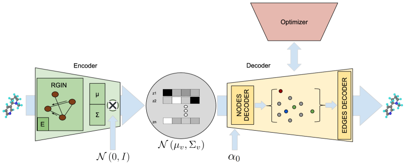
Figure 1: RGCVAE model structure. The encoder feeds the input molecule to a novel relational version of GIN exploiting an edge-specific neural network $E$ that encodes the molecule in the latent space. The decoder receives in input the sampled points and the initial histogram $\bm{\alpha}_{0}$. It decodes the set of sampled points to the unconnected set of atoms, and then it decodes the bonds between them. The optimizer computes an optimized set of latent points which, once decoded, should exhibit better property values.

3.1 Encoder

Let us consider the input graph representation $G$ of a molecule with $m$ atoms. The encoder maps each atom $v\in V$ into a vector sampled by a multivariate normal probability distribution with mean $\ignorespaces\bm{\mu}_{v}$ and variance $\ignorespaces\bm{\sigma}^{2}_{v}$ . To generate these encodings, we define a novel relational variant of GIN, dubbed RGIN, to devise a hidden representation of each atom that embeds the information of its neighboring nodes and of the type of bond connecting them. Our proposed variant is different from the Relational Graph Convolutional Model (R-GCN) presented in Schlichtkrull et al. (2018), as will also be clear from the experimental results reported in the ablation study (Section 7).

In order to consider different types of bonds between atoms, we have changed the original update function of GIN as:

$$\bm{h}_{v}^{(k)}= \text{MLP}^{(k)}\Biggl{(}\left(1+\epsilon^{(k)}\right)\bm{h}_{v}^{(k-1)}$$ (2)

$$+\sum_{u\in\mathcal{N}(v)}\text{MLP}^{(k)}_{\Phi_{e}((v,u))}\left(\bm{h}_{u}^{(k-1)}\right)\Biggr{)},$$

where $\text{MLP}^{(k)}_{\Phi_{e}((v,u))}$ is an edge type specific multi-layer perceptron. The initial hidden representation state for each $v\in V$ is given by $\bm{h}_{v}^{(1)}=W(\Phi_{n}(v))$, where $W:\Theta_{n}\rightarrow\mathbb{R}^{s_{h}}$ is a learnable function which returns a feature vector of size $s_{h}$ for each atom type. Given a latent space of size $s_{\text{lt}}$, $\forall v\in V$, the encoder maps the above hidden states to the target mean $\bm{\mu}_{v}\in\mathbb{R}^{s_{\text{lt}}}$ and variance $\bm{\sigma}^{2}_{v}\in\mathbb{R}^{s_{\text{lt}}}$ vectors via two different MLPs:

$$\bm{\mu}_{v} =\text{MLP}_{\mu}\left(\bm{h}^{(K)}_{v}\right),$$ (3)

$$\text{diag}(\bm{\Sigma}_{v}) =\bm{\sigma}^{2}_{v}=\exp\left(\text{MLP}_{\sigma^{2}}\left(\bm{h}^{(K)}_{v}\right)\right),$$ (4)

where $\bm{\Sigma}_{v}$ defines the covariance matrix where all values, except the diagonal, are set to $0$. It should be emphasized that this model, similarly to CGVAE Liu et al. (2018), generates a probability distribution for each node in the graph, unlike other approaches Gómez-Bombarelli et al. (2018); Kusner et al. (2017); Dai et al. (2018); Jin et al. (2018); Ma et al. (2018); De Cao and Kipf (2018) that generate a probability distribution per molecule.

3.2 Decoder

The decoder is constituted by two main components (see Fig. 1). The first component implements an atom decoding procedure which generates a set of initially unconnected atoms. The second component, that constitutes another novel contribution of this paper, implements an edge decoding procedure, which predicts the presence of an edge between each pair of atoms and the corresponding edge type.

3.2.1 Atom Decoding

The atom decoding procedure receives in input a set of vectors $Z=\{\bm{z}_{v}\}_{v\in[1,m]}$, where each $\bm{z}_{v}$ represents an atom. At the beginning of the generation phase, the $\bm{z}_{v}$’s are sampled from the normal distribution $\ignorespaces\mathcal{N}\left(0,\bm{I}\right)$ , where $\bm{I}$ is the identity matrix, while in training they are obtained from the distribution $\ignorespaces\mathcal{N}\left(\bm{\mu}_{v},\bm{\sigma}^{2}_{v}\right)$ using the reparameterization trick. The atom decoding returns for each $\bm{z}_{v}$ a feature vector $\bm{r}_{v}\in\mathbb{R}^{s_{n}}$ jointly with its atom type $\tau_{v}$, where $s_{n}$ is the dimension of the features. For atom decoding, we adopted the procedure provided in Rigoni et al. (2020a), where the atom type assignment process is conditioned by the previously assigned atom types. However, contrary to Rigoni et al. (2020a), in the generation process we fix the $\alpha_{0}$ histogram for each iteration and we do not sample a new compatible histogram, because the sampling procedure negatively affects some metrics. For more details on the decoding of the atoms, we refer the reader to Appendix D.

3.2.2 Edge Decoding

The edge decoding procedure predicts the presence and type of an edge between each pair of atoms. This procedure receives in input, for each node $v$, the feature vector $\bm{r}_{v}$ with its atom type $\tau_{v}$ returned by the atom decoding step. The process is illustrated in Fig. 2.

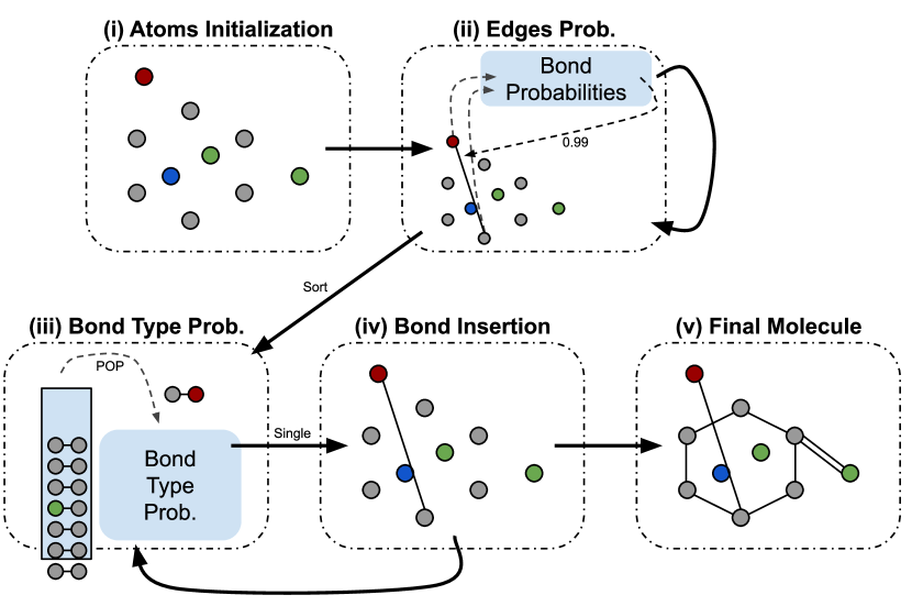
Figure 2: Edge decoder. (i) The atom representations are fed to (ii) a neural network that computes the probability for each pair of atoms to be connected with an edge. Then, (iii) the edges are sorted in descending probability order and are (iv) iteratively added to the partial molecule according to their sampled edge type. (v) The process finishes when all the bonds are added to the molecule.

Given a pair of atoms $(u,v)$ extracted from the set of initially unconnected atoms and their representations $\bm{r}_{u}$ and $\bm{r}_{v}$ (Fig. 2-(i)), two neural networks are used to predict the probability that the two atoms are connected with a bond and the bond type, respectively (Fig. 2-(ii)). Specifically, using the compact notation $\leftrightarrow$ and $\stackrel{{\scriptstyle l}}{{\leftrightarrow}}$ in order to represent the existence of an edge and the existence of an edge of type $l$, respectively, the probability distribution $P\left(v\stackrel{{\scriptstyle l}}{{\leftrightarrow}}u\mid\bm{\phi}_{v,u}\right)$ is:

$$\underbrace{P\left(v\stackrel{{\scriptstyle l}}{{\leftrightarrow}}u\mid\bm{\phi}_{v,u},v\leftrightarrow u\right)}_{\text{Edge type probability}}\underbrace{P\left(v\leftrightarrow u\mid\bm{\phi}_{v,u}\right)}_{\text{Edge probability}},$$ (5)

where

$$\bm{\phi}_{v,u} =\text{Concat}\left(\bm{s}_{v}+\bm{s}_{u},\bm{s}_{v}\odot\bm{s}_{u},\sum_{i=0}^{m-1}\bm{s}_{i}\right),$$ (6)

$$\bm{s}_{v} =\text{Concat}\left(\bm{r}_{v},W(\tau_{v})\right)$$ (7)

$$\bm{s}_{u} =\text{Concat}\left(\bm{r}_{u},W(\tau_{u})\right)$$ (8)

with $\odot$ the component-wise multiplication and $\text{Concat}(\cdot,\cdot)$ is the concatenation function.

Note that $\sum_{i=0}^{m-1}\bm{s}_{i}$ is a global order-invariant representation of all the atoms involved in the sum, and that the obtained matrix containing all the final probabilities is symmetric. In fact, this property is obtained thanks to $\bm{\phi}_{v,u}$ which is defined by only using order invariant representations of the couple of atoms $v$ and $u$. We define the above probability functions as:

$$\begin{aligned} P&\left(v\leftrightarrow u\mid\bm{\phi}_{v,u}\right)=\\ &=\frac{\bm{M}^{e}_{v,u}\odot\exp\left[C\left(\bm{\phi}_{v,u}\right)\right]}{\bm{M}^{e}_{v,u}\odot\exp\left[C\left(\bm{\phi}_{v,u}\right)\right]+1},\end{aligned}$$ (9)

$$\begin{aligned} P&\left(v\stackrel{{\scriptstyle l}}{{\leftrightarrow}}u\mid\bm{\phi}_{v,u},v\leftrightarrow u\right)=\\ &=\frac{\bm{M}^{t}_{v,l,u}\odot\exp\left[L_{l}\left(\bm{\phi}_{v,u}\right)\right]}{\sum_{k}\bm{M}^{t}_{v,k,u}\odot\exp\left[L_{k}\left(\bm{\phi}_{v,u}\right)\right]},\end{aligned}$$ (10)

where both $\mathit{C}\left(\phi\right)$ and $\mathit{L_{l}}\left(\phi\right)$ are MLP neural networks and both $\bm{M}^{e}_{v,u}\in\{0,1\}^{m\times m}$ and $\bm{M}^{t}_{v,k,u}\in\{0,1\}^{m\times d_{e}\times m}$ are binary masks. Specifically, $\bm{M}^{e}_{v,u}$ is a mask not allowing for self loops and edge duplication, while $\bm{M}^{t}_{v,l,u}$ is a mask designated to remove the edges that do not respect the valences law. Let $\nu_{v}$ and $\nu_{u}$ be the valences of atoms $v$ and $u$, respectively, and let $we(l)$ with $l\in\Theta_{e}$ be the function computing the edge weights as follows: 1 for single bonds, 2 for double bonds, and 3 for triple bonds. Then $\bm{M}^{t}_{v,l,u}$ is defined as:

$$\bm{M}^{t}_{v,l,u}=1\iff \bm{M}^{e}_{v,u}=1\,\land\,\nu_{u}\geq we(l)$$ (11)

$$\land\,\nu_{v}\geq we(l).$$

At this point, all the pairs of atoms $(u,v)$, where their probabilities satisfy $P\left(v\leftrightarrow u\mid\bm{\phi}_{v,u}\right)>0.5$, are ordered from the highest to the lowest probability value. Then, the edges are iteratively added one at a time to the atoms according to the type of edge sampled from the distribution $P\left(v\stackrel{{\scriptstyle l}}{{\leftrightarrow}}u\mid\bm{\phi}_{v,u},v\leftrightarrow u\right)$.

If an edge that needs to be added does not respect the chemical constraints, then the model samples, without replacement, a new bond. An edge is discarded only when all the bond types violate the chemical constraints.

At the end of the process (Fig. 2-(v)), all the bonds necessary for the validity of the molecule are completed by adding hydrogen atoms connected to all the atoms whose valences are not correct .

Note that our encoder and edges decoder exhibit the invariant permutation property, while the atom decoder follows the canonical SMILES node order in order to fully exploit the conditioning on valence histograms, which allows to improve the performances on the considered metrics, as demonstrated in the ablation study described in Section 7. It should be stressed that this dependence on the canonical SMILES node order does not affect the capability of the model since the task of generating new molecules does not incur in the graph isomorphism problem. In fact, during the evaluation of the generated molecules, we compare canonical SMILES.

3.3 Property Optimizer

VAE models can incorporate an optimization component to tackle the structure optimization task, which aims to drive the exploration of the latent space towards molecules that exhibit better properties. In the search for new drugs this is very useful as it allows, given a molecule in input, to optimize its structure towards the desired property. Given the set of $m$ sampled latent points $Z=\{\bm{z}_{v}\}_{v\in[1,m]}$ and the histogram $\bm{\alpha}_{0}$, the optimizer $O_{p}(Z,\bm{\alpha}_{0})$ predicts the property $p\in\Theta_{p}$ of the molecule. Specifically, the input points $Z$ and the histogram $\bm{\alpha}_{0}$ are used as input in the first part of the decoder process to generate, for each node $v$, the feature vector $\bm{r}_{v}$ with its atom type $\tau_{v}$. Then the optimizer predicts the property value as:

$$O_{p}(Z,\bm{\alpha}_{0})= \sigma\Biggl{(}\sum_{v=0}^{m-1}\sigma\left(Q^{1}_{p}(\bm{x}_{v})\right)$$ (12)

$$\odot\text{tanh}\left(Q^{2}_{p}(\bm{x}_{v})\right)\Biggr{)},$$

where $\bm{x}_{v}=F\left(\text{Concat}(\bm{r}_{v},\tau_{v})\right)$, $F$ is a single layer neural network with Leaky-ReLU activation function, $Q^{1}_{p}$ and $Q^{2}_{p}$ are linear neural networks with a single layer specific for the property $p$, $\sigma()$ is the sigmoid function and tanh$()$ is the hyperbolic tangent function. At test time, we sample an initial set of latent points $Z$ and an histogram $\bm{\alpha}_{0}$ according to the training set distribution, then we use gradient ascent to reach a set $Z^{\prime}$ of local optimal points.

4 Training

Let us define the graph reconstructed by the decoder as $\tilde{G}=(\tilde{V},\tilde{E},\tilde{\Phi_{e}},\tilde{\Phi_{n}})$, which can be represented by the predicted adjacency matrix $\tilde{\bm{A}}\in\mathbb{R}_{[0,1]}^{m\times m}$, edge type tensor $\tilde{\bm{E}}\in\mathbb{R}_{[0,1]}^{m\times m\times d_{e}}$, node attribute matrix $\tilde{\bm{F}}\in\mathbb{R}_{[0,1]}^{m\times d_{n}}$ and vector of molecule properties $\tilde{\bm{p}}\in\mathbb{R}^{d_{p}}$. During generation, these matrices are obtained sampling from the decoder’s output probabilities, while during training they are obtained using the argmax function. The order in which the vertices appear in the matrices is given by the ordering imposed by the SMILES Weininger (1988) coding.
Let $\bm{\mu}$ and $\bm{\sigma}^{2}$ be the matrices formed respectively by the $m$ means $\{\bm{\mu}_{v}\}_{v\in[1,m]}$ and variances $\{\bm{\sigma}^{2}_{v}\}_{v\in[1,m]}$ predicted by the encoder. Let $\bm{Z}\sim\mathcal{N}\left(\bm{\mu},\bm{\sigma}^{2}\right)$ be the matrix formed by the $m$ latent space sampled points $Z=\{\bm{z}_{v}\}_{v\in[1,m]}$, then the loss function to minimize is $\mathcal{L}(G,\tilde{G},\bm{\mu},\bm{\sigma}^{2})$, defined as:

$$\mathcal{L}(G,\tilde{G},\bm{\mu},\bm{\sigma}^{2})= \mathcal{L}_{rec}(G,\tilde{G})+\lambda_{1}\mathcal{L}_{lt}(\bm{\mu},\bm{\sigma}^{2})$$ (13)

$$+\lambda_{2}\mathcal{L}_{opt}(\bm{p},\tilde{\bm{p}}),$$

where $\ignorespaces\lambda_{1}$ and $\ignorespaces\lambda_{2}$ are trade-off hyper-parameters, $\ignorespaces\mathcal{L}_{rec}$ is the reconstruction loss, $\ignorespaces\mathcal{L}_{lt}$ is the variational autoencoder Kullback–Leibler (KL) loss, and $\ignorespaces\mathcal{L}_{opt}$ is the loss defined on the basis of the property to predict, referred to as optimization loss in the literature since it can be used to drive the generation of molecules towards molecules with better values for the property of choice. In more detail, $\mathcal{L}_{rec}$ is defined as:

$$\mathcal{L}_{rec}(G,\tilde{G})= \mathcal{L}_{a}(\bm{F},\tilde{\bm{F}})+\mathcal{L}_{b}(\bm{A},\tilde{\bm{A}})$$ (14)

$$+\mathcal{L}_{tb}(\bm{E},\tilde{\bm{E}}),$$

where $\mathcal{L}_{a}$, $\mathcal{L}_{tb}$, and $\mathcal{L}_{b}$ are cross-entropy losses:

$$\begin{aligned} \mathcal{L}_{a}(\bm{F},\tilde{\bm{F}})=-\sum_{v=0}^{m-1}\sum_{t=0}^{d_{n}-1}\log(\tilde{\bm{F}}_{v,t})\odot\bm{F}_{v,t},\end{aligned}$$ (15)

$$\begin{aligned} \mathcal{L}_{tb}(\bm{E},\tilde{\bm{E}})=&-\sum_{v=0}^{m-1}\sum_{u=0}^{m-1}\underbrace{\bm{A}_{v,u}}_{\text{Teacher forcing}}\\ &\odot\Biggl{(}\sum_{t=0}^{d_{e}-1}\log({\tilde{\bm{E}}_{v,u,t}})\odot\bm{E}_{v,u,t}\Biggr{)}\end{aligned}$$ (16)

$$\begin{aligned} \mathcal{L}_{b}(\bm{A},\tilde{\bm{A}})=&-\sum_{v=0}^{m-1}\sum_{u=0}^{m-1}\Biggl{(}\log(1-\tilde{\bm{A}}_{v,u})\\ &\odot(1-\bm{A}_{v,u})+\log(\tilde{\bm{A}}_{v,u})\Biggr{)}\end{aligned}$$ (17)

Note that the loss $\mathcal{L}_{tb}$ uses teacher forcing to calculate the bond-type loss only where the bond exists in the molecule. The variational autoencoder loss Kullback–Leibler is defined as:

$$\mathcal{L}_{lt}(\bm{\mu},\bm{\sigma}^{2})= -\frac{1}{2}\sum_{i=0}^{m-1}\sum_{j=0}^{s_{\text{lt}}-1}1+\log(\bm{\sigma}^{2}_{i,j})$$ (18)

$$-\bm{\mu}_{i,j}^{2}-\bm{\sigma}^{2}_{i,j},$$

while the optimization loss $\mathcal{L}_{opt}$ is defined as:

$$\mathcal{L}_{opt}(\bm{p},\tilde{\bm{p}})=\sum_{p=1}^{d_{p}}\dfrac{(\tilde{\bm{p}_{p}}-\bm{p}_{p})^{2}}{2}.$$ (19)

5 Related Works

Follow related works that tackle the distribution learning task.

Focusing on VAE approaches, Character VAE Gómez-Bombarelli et al. (2018) exploits, in input and output, SMILES strings describing the structure of the molecule. The encoder uses a convolutional network and the decoder uses a gated recurrent unit (GRU). Grammar VAE Kusner et al. (2017) adds to Character VAE a context-free grammar, to guide the correct generation of SMILES strings. Syntax Directed VAE Dai et al. (2018) improves Grammar VAE using a more expressive grammar,the attribute grammar Knuth (1968), which aims to generate strings that not only are syntactically valid, but also semantically reasonable. Junction Tree VAE Jin et al. (2018) represents molecules using graphs, composed of chemical substructures that are extracted from the training set. New molecular graphs are obtained by first generating a tree-structured scaffold formed by substructures, and then combining the substructures together using a graph message passing network. HierVAE Jin et al. (2020) uses a hierarchical graph encoder-decoder that employs large and flexible graph motifs as basic building blocks to encode and decode a molecule. Podda et al. (2020) generates molecules fragment by fragment instead of atom by atom, using a language model based on the SMILES representation of molecules. Regularized Graph VAE Ma et al. (2018) casts the molecule generation problem as a constrained optimization problem, where chemical constraints are encoded in the VAE loss function. Constrained Graph VAE (CGVAE) Liu et al. (2018) encodes in the latent space single atoms rather than whole molecules. To generate a molecule, first the model samples several nodes in the latent space and assigns them an atom type using a linear classifier; then it connects them using a constrained breadth first algorithm. Both the encoder and decoder are implemented by a gated graph sequence neural network, that makes the model computationally heavy to train. CCGVAE Rigoni et al. (2020a) extends CGVAE conditioning only the decoder with the histogram of valences of the molecule’s atoms. In particular, the decoder takes in input several nodes sampled in the latent space together with a histogram of valence, and for each of those points, it assigns its atom type applying an iterative procedure that depends on the histogram of valences.

CCGVAE model is the one most related to our proposal as we also condition the decoder with the histogram of valence information. However, our RGCVAE architecture is completely different from that of CCGVAE. In fact, in our model, we have an encoder that exploits the newly defined representations of molecules using the new relational GIN component. Furthermore, the decoder does not contain a convolutional operator which is instead present in CCGVAE. Finally, our optimization component does not optimize points directly from latent space, but predicts scores from the internal states of the decoder component.

Focusing on the generative adversarial approach, MolGAN De Cao and Kipf (2018), learns via reinforcement learning to directly reconstruct small organic molecules, by predicting directly the atoms type, and the existence of bonds (and their types). NeVAE Samanta et al. (2019) predicts the spatial coordinates of the atoms of the generated molecules, and optimizes them to improve its structures.

Focusing on the Flow-based models, GraphAF Shi et al. (2019) combines the advantages of both autoregressive and flow-based approaches in order to model the data density estimation, while MolGrow Kuznetsov and Polykovskiy (2021) uses a hierarchical normalizing flow-based model for generating molecular graphs. MoFlow Zang and Wang (2020) generates molecular graphs by first generating bonds through a Glow based model, then by generating atoms given bonds by a novel graph conditional flow-based model.

Regarding the evaluation process adopted in this work, we embrace the same testbed environment defined in Rigoni et al. (2020b) to compare our results with many other state-of-the-art models objectively.

6 Experiments

Following Rigoni et al. (2020b, a), we compared our RGCVAE to several state-of-the-art Variational Autoencoder proposals considering different metrics on two widely adopted datasets. Specifically, focusing on the distribution learning task, for each model we assessed the ability to reconstruct the input molecules and the ability to generate new ones.

6.1 Experimental setup

Following Rigoni et al. (2020b), we evaluated our model on two widely used datasets: QM9 Ruddigkeit et al. (2012); Ramakrishnan et al. (2014), which includes $\sim$134,000 organic molecules with at most 9 atoms, and ZINC Irwin and Shoichet (2005), which includes 250,000 drug-like molecules with at most 38 atoms. More details on the datasets are reported in Appendix A. We use for each model the same training, validation and test splits as in Rigoni et al. (2020b).

We considered the following metrics: (i) Reconstructionthat, given an input molecule and a set of generated molecules, computes the percentage of generated molecules that are equal to the one in input. This is calculated on the test set; (ii) Validitythat, given a set of generated molecules, represents the percentage of them that is valid, i.e. that represent actual molecules; (iii) Noveltythat represents the percentage of generated molecules not in the training set; (iv) Uniquenessthat represents (in percentage) the ability of the model to generate different molecules in output, and is computed as the size of the unique set of valid generated molecules divided by the total number of valid generated molecules; (v) Diversitythat measures how much the generated molecules are different from those in the training set (comparing randomly selected substructures). (vi) Quantitative Estimation Drug-likeness (QED)which indicates in percentage how likely it is that the molecule is a good candidate to become a drug. We used this metric to evaluate the optimization procedure. Reconstruction is computed on $5,000$ test set molecules encoded and decoded 20 times, while the other metrics are computed sampling $20,000$ points from the standard normal distribution and decoding each point once.

Notice that in our model we deal with molecules defined with stereochemistry information, and for this reason, during the evaluation of the Reconstruction metric, we always compare the canonical SMILES representation. Some works in literature compare graph representations that do not contain such information or they clean the SMILES representation before training/evaluation phase. We refer the reader to Section 7 to more details.

The experiments on the QM9 dataset were performed on a PC with an Intel(R) i9 9900k CPU, 32 GB of RAM and a Quadro RTX 4000 GPU with 8GB of memory. For the experiments on the ZINC dataset we used a server with 2 Intel(R) Xeon(R) E5-2650a CPUs, 160 GB of RAM and a Tesla T4 GPU with 15GB of memory. Regarding the model selection process, we started from a model where each neural network component of RGCVAE was implemented as a linear transformation and then, according to the obtained reconstruction error on the validation set, we iteratively added hidden layers to each neural network. When adding depth to the networks did not improve the reconstruction metric anymore, we used a grid search to find the best value for the $\lambda_{1}$ parameter which controls the importance of the Kullback–Leibler divergence in the model loss. The network, as shown in Section 7, is sensitive with respect to this parameter that trades off between reconstruction on one hand, and uniqueness and novelty on the other hand.

Due to limitations in the available computational resources, we did not fine-tune the other parameters. The results presented in this section are computed on the test set with the best model obtained in the model selection process. More details on the model selection procedure are reported in Appendix E.

The approaches proposed in literature are evaluated using different metrics and on different datasets or variations of them.

For this reason, it was necessary to reproduce the baseline results to calculate all the metrics in the datasets considered in this paper. For each baseline model, we used the official code and set the hyper-parameters to the values specified by the authors. Consequentially, we have trained and tested each baseline only on the datasets originally considered by the authors and adopted in this work. In Appendix B, we report for a reference the results obtained by the baseline models in the datasets considered in this paper that where originally not considered by the authors, while Appendix C presents results considering the molecules properties.

Table 2: Average and standard deviation (where applicable) of different evaluation metrics on the QM9 datasets.

Model	Reconstruction	Validity	Novelty	Uniqueness	Diversity	Time
Graph VAE	13.6	80.1	45.6	88.1	66.2	01m
	$\ignorespaces\pm$ 34.3	$\ignorespaces\pm$ 32.4	$\ignorespaces\pm$ 49.8		$\ignorespaces\pm$ 28.0
Reg. GVAE	7.3	91.8	49.8	77.1	68.7	01m
	$\ignorespaces\pm$ 26.0	$\ignorespaces\pm$ 27.5	$\ignorespaces\pm$ 50.0		$\ignorespaces\pm$ 25.6
CGVAE	24.5	100	92.8	98.3	76.1	21m
	$\ignorespaces\pm$ 27.9	$\ignorespaces\pm$ 0	$\ignorespaces\pm$ 19.1		$\ignorespaces\pm$ 22.6
CCGVAE	55.4	100	88.5	93.2	79.2	1.5h
	$\ignorespaces\pm$ 49.7	$\ignorespaces\pm$ 0	$\ignorespaces\pm$ 31.9		$\ignorespaces\pm$ 22.0
RGCVAE (ours)	94.8	99.9	96.4	94	87.7	01m
	$\ignorespaces\pm$ 22.2	$\ignorespaces\pm$ 3.5	$\ignorespaces\pm$ 18.7		$\ignorespaces\pm$ 19.2

Table 3: Average and standard deviation (where applicable) of different evaluation metrics on the ZINC dataset.

Model	Reconstruction	Validity	Novelty	Uniqueness	Diversity	Time
Char. VAE	25.3	0.9	100	91.4	98.2	07m
	$\ignorespaces\pm$ 43.5	$\ignorespaces\pm$ 9.6	$\ignorespaces\pm$ 0		$\ignorespaces\pm$ 7.0
Gram. VAE	55.8	5.1	100	94.6	99.2	21m
	$\ignorespaces\pm$ 49.7	$\ignorespaces\pm$ 23.0	$\ignorespaces\pm$ 0		$\ignorespaces\pm$ 4.5
SD VAE	77.4	19.0	100		93.6	24m
	$\ignorespaces\pm$ 41.8	$\ignorespaces\pm$ 39.2	$\ignorespaces\pm$ 0	100	$\ignorespaces\pm$ 18.5
JT VAE	50.2	99.6	99.9	99.7	33.0	55m
	$\ignorespaces\pm$ 50.0	$\ignorespaces\pm$ 6.35	$\ignorespaces\pm$ 1.2		$\ignorespaces\pm$ 21.78
CGVAE	0.4	100	100	99.9	66.0	15.5h
	$\ignorespaces\pm$ 5.9	$\ignorespaces\pm$ 0	$\ignorespaces\pm$ 0		$\ignorespaces\pm$ 22.8
CCGVAE	22.2	100	100	92.8	80.0	21.5h
	$\ignorespaces\pm$ 41.5	$\ignorespaces\pm$ 0	$\ignorespaces\pm$ 0		$\ignorespaces\pm$ 16.7
RGCVAE (ours)	79.7	99.9	100	61.1	98.9	12m
	$\ignorespaces\pm$ 40.2	$\ignorespaces\pm$ 1.2	$\ignorespaces\pm$ 0		$\ignorespaces\pm$ 5.0

6.2 Reconstruction and Generation

Table 2 and Table 3 report the average and standard deviation of the results obtained by the models on the QM9 and ZINC datasets, respectively . Moreover, they report the computational time required to perform one training epoch. In general, all the metrics adopted in this work, capture different but important aspects of the molecule generation process. Ideally, a model should perform well in all such metrics. Having even only one of them very low indicates a strong limitation of such model. In particular, VAE models usually trade-off the capability of the model of reconstructing the molecule in input with the capability of the model of generating new valid, novel and useful molecules. For instance, MOSES Polykovskiy et al. (2018), that does not adopt the reconstruction metric in its evaluation process, presents very high validity, novelty, and uniqueness values for Character VAE Gómez-Bombarelli et al. (2018) and AAE Kadurin et al. (2017). However, our evaluation of reconstruction for the models released by MOSES’ authors returned values very close to zero for each of these two models. In fact, authors report in the official MOSES’s GitHub repository that the obtained models suffer by the posterior collapse problem. This means that the encoding process is not contributing to the generation process, which raises many doubts on how much the generated molecules follow the training set distribution.

In our evaluation process, for each model, we have used the official code and the hyper-parameter values provided by the authors. However, we could not reproduce the 76.7% reconstruction of the JTVAE model. Many users pointed out bugs in the code, and they also claimed not being able to achieve the values reported in the original work. We thus consider the results in the JTVAE paper not reproducible.

Considering our results, we notice that methods that are based on SMILES strings instead of graphs (i.e. Character VAE, Grammar VAE and Syntax Directed VAE) perform poorly. Specifically, the validity of the generated strings is very low, i.e. the networks struggle to generate strings that are valid SMILES. Thus, even though on some metrics these models perform pretty well, they are not well suited for the task of molecule generation. Methods that use the graph representation of molecules show higher performance. Among them, our model (RGCVAE) presents very good results in both the QM9 and ZINC datasets. In particular, on the QM9 dataset, when compared to the best baseline model (CCGVAE considering all the metrics), RGCVAE improves its Reconstruction by almost 39%. On the ZINC dataset, RGCVAE reconstruction is 29.5% higher than JTVAE (3% considering the original results reported by the authors) and 55.5% higher than CCGVAE. Notwithstanding the good Reconstruction results, RGCVAE also shows high values in the Validity, Novelty, Uniqueness and Diversity metrics on both the datasets. The only metric where RGCVAE is not among the best performing methods is the Uniqueness on the ZINC dataset, which is lower compared to JTVAE and CCGVAE. We argue that this relatively low Uniqueness value is a consequence of the well-formed latent space of the model amenable to the high Reconstruction value. In Section 7, we show that sacrificing the model Reconstruction capabilities the model reaches higher Uniqueness values. Notice, however, that both CCGVAE and JTVAE show a much lower Diversity compared to RGCVAE, which indicates that the generated molecules are built with really (98.9% on ZINC) different sub-structures than those that form the molecule’s training set.

Concerning the computational efficiency, we can observe that the models that use the SMILES representation, i.e. the first three models in each table, tend to be faster to train than the ones that use the molecular graph representation, i.e. all the others. However, as stated before, their predictive performances are generally low. The high computational time and resources required by some models for completing a training epoch, e.g. CGVAE and CCGVAE, limits the number of epochs that can be performed for training them in a reasonable amount of time. This may hurt their predictive performances. While Graph VAE, Regularized GVAE

tend to be fast, Graph VAE and Regularized GVAE present low Reconstruction and Novelty values.

From these tables, we can notice that our proposed RGCVAE model is among the fastest methods. Overall, our proposed model is very efficient while being at the-state-of-the-art in several metrics.

6.3 Property Optimization

This task aims to optimizing molecules structures towards desired properties. Following Jin et al. (2018), starting from a set of points sampled in the latent space and an initial histogram of valences, the optimization algorithm performs gradient ascent moving the representations toward molecules that maximizes the QED property, as described in Section 3.3.

In Fig. 3, we present an example of QED optimization on the ZINC dataset. Starting from left, we can see the sampled molecule and the molecules obtained at each optimization time step. We report the real QED values, from which we can see that the model is able to improve the molecule structure towards those that improve the QED value.

Figure 3: Example of QED-directed optimization performed in the model latent space trained on the ZINC dataset. (i) is the initially sampled molecule, while (ii)-(iv) are the molecules obtained at each optimization step.

7 Ablation Study

In this section, we present an ablation study to validate the different components of RGCVAE. Specifically, we analyze the impact on the predictive performance of the atom encoding (different choices are possible), of the Relational GIN over a standard GIN and the R-GCN Schlichtkrull et al. (2018) in the encoder (Section 3.1), and of the use of the histograms of valence (Section 3.2).

Table 4: Minimum reconstruction errors that is possible to achieve with different graph representations.

Representation	Atom	Valence	Charge	Chiral	%QM9	%ZINC
1	✔	✖	✖	✖	22.83	72.32
2	✔	✔	✔	✖	1.70	63.08
3	✔	✔	✔	✔	1.70	7.76

In our work, we deal with molecules that include the stereochemistry relative spatial arrangement of atoms in the molecules. For this reason, when the molecule is converted as a graph representation, it is necessary to store, learn, and predict these information to build back the original molecule, otherwise sometimes it is not possible to reconstruct the original molecule. This makes the learning process more difficult. Notice that many models in literature do not consider this information, and they just compare molecules using their graph representations or SMILES strings Zang and Wang (2020), where the stereochemistry information is removed, leading to higher Reconstruction values than those reported in this work. Moreover, this information is often only reported in the code, not in the paper. In order to reach the maximum Reconstruction value and do not occur in low values due to the lack of information in the molecule’s graph representation, we have considered three atom representations: 1. atom type, e.g. “C” for carbon; 2. atom type, total valence and formal charge, e.g. “C4(0)” for carbon atom with total valence 4 and formal charge 0; 3. atom type, total valence, formal charge, presence of chiral property, e.g. “O3(1)0” for an oxygen atom with valence 3, formal charge 1 and without the chiral property.

Table 4 reports the minimum Reconstruction error that is possible to achieve using these representations on the two adopted datasets. It is clear that the third representation is the one that better captures the molecule structure information (including the stereochemistry information). In fact, the third representation provided the best performance for our model. Moreover, we verified the importance of using the Relational GIN in the encoder, and the histograms in the decoding procedure.

Table 5: This table reports the ablation study results obtained by our RGCVAE model.

			QM9					ZINC
Rep.	Hist.	Encoding Network	Rec.	Val.	Nov.	Uniq.	Div.	Rec.	Val.	Nov.	Uniq.	Div.
1	✖	RGIN	68.8	100	77.9	84.1	69.95	20.11	99.9	100	1.9	100
			$\ignorespaces\pm$ 46.3	$\ignorespaces\pm$ 0	$\ignorespaces\pm$ 41.5		$\ignorespaces\pm$ 27.6	$\ignorespaces\pm$ 40.1	$\ignorespaces\pm$ 1.7	$\ignorespaces\pm$ 0		$\ignorespaces\pm$ 0.1
1	✔	RGIN	76.2	99.9	95.8	90.4	87.7	27.1	97.0	100	90.3	96.5
			$\ignorespaces\pm$ 42.6	$\ignorespaces\pm$ 3.2	$\ignorespaces\pm$ 20.1		$\ignorespaces\pm$ 19.4	$\ignorespaces\pm$ 44.5	$\ignorespaces\pm$ 17.0	$\ignorespaces\pm$ 0		$\ignorespaces\pm$ 9.2
3	✖	RGIN	85.9	100	78.1	83.9	69.6	47.4	100	100	2.4	100
			$\ignorespaces\pm$ 34.8	$\ignorespaces\pm$ 0	$\ignorespaces\pm$ 41.4		$\ignorespaces\pm$ 28.2	$\ignorespaces\pm$ 49.9	$\ignorespaces\pm$ 0	$\ignorespaces\pm$ 0		$\ignorespaces\pm$ 0
3	✔	RGIN	94.8	99.9	96.36	94.0	87.7	79.7	99.9	100	61.1	98.9
			$\ignorespaces\pm$ 22.21	$\ignorespaces\pm$ 3.5	$\ignorespaces\pm$ 18.7		$\ignorespaces\pm$ 19.2	$\ignorespaces\pm$ 40.2	$\ignorespaces\pm$ 1.2	$\ignorespaces\pm$ 0		$\ignorespaces\pm$ 4.98
3	✔	GIN	41.6	99.3	94.1	87.2	87.47	54.0	100	100	42.2	99.8
			$\ignorespaces\pm$ 49.3	$\ignorespaces\pm$ 8.5	$\ignorespaces\pm$ 23.5		$\ignorespaces\pm$ 19.9	$\ignorespaces\pm$ 49.8	$\ignorespaces\pm$ 0	$\ignorespaces\pm$ 0		$\ignorespaces\pm$ 2.14
3	✔	R-GCN	86.0	99.8	95.5	89.1	88.5	64.9	100	100	81.53	96.44
			$\ignorespaces\pm$ 34.7	$\ignorespaces\pm$ 4.1	$\ignorespaces\pm$ 20.76		$\ignorespaces\pm$ 19.41	$\ignorespaces\pm$ 47.7	$\ignorespaces\pm$ 0	$\ignorespaces\pm$ 0		$\ignorespaces\pm$ 9.41

Table 5 reports the results obtained by different versions of our model, including or not the histogram of valences, the use of a standard GIN network or a standard R-GCN network over the novel Relational GIN for the encoder, and using either representation 1 or 3, i.e. the simplest and the most sophisticated representation.

We evaluated the effectiveness of the Relational GIN only on the best performing representation 3. To make a fair comparison, we have selected the model that has the higher Reconstruction value on the validation set among 200 epochs for each dataset.

From tables it is evident that using the histogram of valences to condition the decoder improves the model ability in both the reconstruction and the generation tasks. In fact, on the QM9 dataset, it improves the Reconstruction values by $\sim$7% when using representation 1, and above $8\%$ when using representation 3. A similar improvement is observed also for the Uniqueness metric, although in a reduced form for representation 1. We can observe the same behaviour on the ZINC dataset.

Notice that, using both representation 1 and 3, if the model does not use the histogram of valences, the Uniqueness values are very low. We argue that these improvements are due to the fact that using the histogram of valences: (i) in reconstruction, drives the generation process toward molecules with a valence distribution closer to the ones of the molecules in the training set; (ii) in generation, drastically decreases the KL divergence loss, which means that the latent space is closer to the standard normal distribution, i.e. the distribution from which the generated latent representations are sampled.

From the results, it is also clear that the Relational GIN dramatically improves the performance over the versions using the standard GIN and the R-GCN. Regarding the expressiveness of the different types of atom representation, as it was expected, the results improve with atom representation 3.

Finally, in Table 6 we report the results of our model when changing value of the $\lambda_{1}$ hyper-parameter. As expected, increasing the value leads to lower values of Reconstruction while improving in many cases the other metrics.

Table 6: This table reports the ablation study results obtained by our RGCVAE model as the $\lambda_{1}$ hyper-parameter value changes.

	QM9					ZINC
$\bm{\lambda_{1}}$	Rec.	Val.	Nov.	Uniq.	Div.	Rec.	Val.	Nov.	Uniq.	Div.
0.01	96.5	99.5	95.4	90.9	79.9	79.7	99.9	100	61.1	98.9
	$\ignorespaces\pm$ 18.3	$\ignorespaces\pm$ 7.9	$\ignorespaces\pm$ 20.9		$\ignorespaces\pm$ 23.2	$\ignorespaces\pm$ 40.2	$\ignorespaces\pm$ 1.2	$\ignorespaces\pm$ 0		$\ignorespaces\pm$ 5.0
0.05	94.8	99.9	96.4	94.0	87.7	62.2	99.9	100	99.8	92.9
	$\ignorespaces\pm$ 22.2	$\ignorespaces\pm$ 3.5	$\ignorespaces\pm$ 18.7		$\ignorespaces\pm$ 19.2	$\ignorespaces\pm$ 48.5	$\ignorespaces\pm$ 1.9	$\ignorespaces\pm$ 0		$\ignorespaces\pm$ 13.0
0.1	93.3	99.9	97.1	95.2	90.4	55.62	99.9	100	86.5	97.9
	$\ignorespaces\pm$ 25.0	$\ignorespaces\pm$ 3.0	$\ignorespaces\pm$ 16.7		$\ignorespaces\pm$ 17.4	$\ignorespaces\pm$ 49.7	$\ignorespaces\pm$ 0.7	$\ignorespaces\pm$ 0		$\ignorespaces\pm$ 7.0
0.2	83.5	99.9	96.6	87.3	93.0	40.0	99.9	100	99.9	94.9
	$\ignorespaces\pm$ 37.18	$\ignorespaces\pm$ 3.4	$\ignorespaces\pm$ 18.2		$\ignorespaces\pm$ 15.2	$\ignorespaces\pm$ 49.0	$\ignorespaces\pm$ 1.0	$\ignorespaces\pm$ 0		$\ignorespaces\pm$ 10.2

8 Conclusions and Future Works

This paper introduced RGCVAE, a VAE deep generative model for molecule generation. The main features of RGCVAE are: (i) an improved reconstruction error with respect to state-of-the-art VAE models; (ii) a very efficient runtime, both in training and in generation. These features are obtained thanks to the novel contributions of this paper, i.e. an extension of the GIN model for relational data, RGIN, exploited during the encoding phase, and a new and efficient decoder which allows to effectively generate novel molecules. In order to validate the usefulness of the different information sources exploited by the model, we have performed an ablation study that confirmed the goodness of the choices made. We have compared our model results against several VAE models in literature, considering many metrics on two widely adopted datasets. Results show that RGCVAE perform state-of-the-art molecule generation performance while being significantly faster to train.

Future works will aim at improving the model by understanding how to embed further knowledge priors into both the encoder and decoder.

Appendix A

A.1 Dataset Details

Table 7: Statistics about the QM9 and ZINC datasets.

Dataset	#Molecules	#Atoms	#Atom Types	#Bond Types
QM9	134K	9	4	3
ZINC	250K	38	9	3

As presented in the main article, Table 7 synthetically reports the main characteristics of the QM9 and ZINC datasets used for the evaluations. Both use the same number of bond types, but they differ in the number of atom types, i.e. 4 for QM9 and 9 for ZINC, and atom per molecules, i.e. at maximum 9 for QM9 and 38 for ZINC.

Appendix B

B.1 Model Results

Table 8: Average and standard deviation (where applicable) of different evaluation metrics on the QM9 and ZINC data-sets. The symbols ’‡’ and ’†’ denote models where we used values for the hyper-parameters tuned by the authors. Specifically, ’‡’ refers to the QM9 dataset, while ’†’ refers to the ZINC dataset.

	QM9 dataset						ZINC dataset
Model	Rec.	Val.	Nov.	Uniq.	Div.	Time	Rec.	Val.	Nov.	Uniq.	Div.	Time
Char. VAE†	49.9	5.9	92.2	94.8	91.3	02m	25.3	0.9	100	91.4	98.2	07m
	$\ignorespaces\pm$ 50.0	$\ignorespaces\pm$ 23.5	$\ignorespaces\pm$ 26.8		$\ignorespaces\pm$ 18.9		$\ignorespaces\pm$ 43.5	$\ignorespaces\pm$ 9.6	$\ignorespaces\pm$ 0		$\ignorespaces\pm$ 7.0
Gram. VAE†	86.2	12.6	84.0	59.3	98.7	07m	55.8	5.1	100	94.6	99.2	21m
	$\ignorespaces\pm$ 34.5	$\ignorespaces\pm$ 33.2	$\ignorespaces\pm$ 36.7		$\ignorespaces\pm$ 6.7		$\ignorespaces\pm$ 49.7	$\ignorespaces\pm$ 23.0	$\ignorespaces\pm$ 0		$\ignorespaces\pm$ 4.5
SD VAE†	97.5	16.0	100		99.6	04m	77.4	19.0	100		93.6	24m
	$\ignorespaces\pm$ 16.0	$\ignorespaces\pm$ 36.7	$\ignorespaces\pm$ 0	100	$\ignorespaces\pm$ 1.1		$\ignorespaces\pm$ 41.8	$\ignorespaces\pm$ 39.2	$\ignorespaces\pm$ 0	100	$\ignorespaces\pm$ 18.5
Graph VAE‡	13.6	80.1	45.6	88.1	66.2	01m	0.3	62.6	100		71.5	18m
	$\ignorespaces\pm$ 34.3	$\ignorespaces\pm$ 32.4	$\ignorespaces\pm$ 49.8		$\ignorespaces\pm$ 28.0		$\ignorespaces\pm$ 4.6	$\ignorespaces\pm$ 48.4	$\ignorespaces\pm$ 0	100	$\ignorespaces\pm$ 25.4
Reg. GVAE‡	7.3	91.8	49.8	77.1	68.7	01m	0.0	86.5	100	90.3	97.9	19m
	$\ignorespaces\pm$ 26.0	$\ignorespaces\pm$ 27.5	$\ignorespaces\pm$ 50.0		$\ignorespaces\pm$ 25.6		$\ignorespaces\pm$ 0.8	$\ignorespaces\pm$ 34.2	$\ignorespaces\pm$ 0		$\ignorespaces\pm$ 7.0
JT VAE†	23.7	99.9	87.7	89.5	60.9	1.7h	50.2	99.6	99.9	99.7	33.0	55m
	$\ignorespaces\pm$ 42.5	$\ignorespaces\pm$ 2.7	$\ignorespaces\pm$ 32.8		$\ignorespaces\pm$ 29.5		$\ignorespaces\pm$ 50.0	$\ignorespaces\pm$ 6.35	$\ignorespaces\pm$ 1.2		$\ignorespaces\pm$ 21.78
CGVAE‡, †	24.5	100	92.8	98.3	76.1	21m	0.4	100	100	99.9	66.0	15.5h
	$\ignorespaces\pm$ 27.9	$\ignorespaces\pm$ 0	$\ignorespaces\pm$ 19.1		$\ignorespaces\pm$ 22.6		$\ignorespaces\pm$ 5.9	$\ignorespaces\pm$ 0	$\ignorespaces\pm$ 0		$\ignorespaces\pm$ 22.8
CCGVAE‡, †	55.4	100	88.5	93.2	79.2	1.5h	22.2	100	100	92.8	80.0	21.5h
	$\ignorespaces\pm$ 49.7	$\ignorespaces\pm$ 0	$\ignorespaces\pm$ 31.9		$\ignorespaces\pm$ 22.0		$\ignorespaces\pm$ 41.5	$\ignorespaces\pm$ 0	$\ignorespaces\pm$ 0		$\ignorespaces\pm$ 16.7
RGCVAE (ours)	94.8	99.9	96.4	94	87.7	01m	79.7	99.9	100	61.1	98.9	12m
	$\ignorespaces\pm$ 22.2	$\ignorespaces\pm$ 3.5	$\ignorespaces\pm$ 18.7		$\ignorespaces\pm$ 19.2		$\ignorespaces\pm$ 40.2	$\ignorespaces\pm$ 1.2	$\ignorespaces\pm$ 0		$\ignorespaces\pm$ 5.0

As explained in the main document, very often the models in the literature do not use all the same datasets and metrics considered in this work, and for this reason, it was necessary to reproduce the baseline results to calculate all the metrics. For each model, we always used the official code with the hyper-parameters specified by the authors to reproduce the baselines’ results. In Table 8 we have reported all the results obtained also in the datasets not originally considered by the authors. Notice that we did not perform an extensive hyper-parameter search in these new datasets.

Appendix C

C.1 Evaluating Molecule Properties

We have performed additional evaluations on the presented RGCVAE. Specifically, we have explored the properties of the molecules generated by the model as done for Rigoni et al. (2020b, a) using some common metrics used in this area of research:

1. Natural Product (NP) which indicates how much the generated molecules structural space is similar to the one covered by natural products Ertl et al. (2008);

2. Solubility (Sol.) which indicates how much a molecule is soluble in water, an important property for drugs;

3. Synthetic Accessibility Score (SAS) which represents how easy (0) or difficult (100) it is to synthesize a molecule;

4. Quantitative Estimation Drug-likeness (QED) which indicates in percentage how likely it is that the molecule is a good candidate to become a drug.

We report the results about our experiments in Table 9. The table reports the evaluations of the properties and the number of epochs used for the training of each model. Moreover, the last row reports the average values of the properties for each dataset.

Table 9: Average and standard deviation (where applicable) of different evaluation metrics on the QM9 and ZINC data-sets. The symbols ’‡’ and ’†’ denote models where we used values for the hyper-parameters tuned by the authors. Specifically, ’‡’ refers to the QM9 dataset, while ’†’ refers to the ZINC dataset.

Model trained on QM9	$\uparrow$%NP	$\uparrow$%Sol.	$\downarrow$%SAS	$\uparrow$%QED	T.*Epoch	N.Epochs
Character VAE	88.79	46.55	29.10	30.02	00h:02m	100
	$\ignorespaces\pm$ 11.74	$\ignorespaces\pm$ 32.71	$\ignorespaces\pm$ 28.52	$\ignorespaces\pm$ 19.55
Grammar VAE	83.34	35.85	52.3	35.18	00h:07m	100
	$\ignorespaces\pm$ 15.45	$\ignorespaces\pm$ 19.46	$\ignorespaces\pm$ 31.63	$\ignorespaces\pm$ 11.53
Syntax Directed VAE	88.89	26.2	14.65	31.37	00h:04m	500
	$\ignorespaces\pm$ 10.64	$\ignorespaces\pm$ 22.26	$\ignorespaces\pm$ 35.15	$\ignorespaces\pm$ 11.18
Graph VAE‡	94.71	35.92	29.72	48.25	00h:01m	200
	$\ignorespaces\pm$ 10.82	$\ignorespaces\pm$ 13.49	$\ignorespaces\pm$ 28.27	$\ignorespaces\pm$ 9.53
Regularized GVAE‡	95.77	39.38	30.58	48.79	00h:01m	150
	$\ignorespaces\pm$ 9.26	$\ignorespaces\pm$ 14.52	$\ignorespaces\pm$ 24.69	$\ignorespaces\pm$ 7.83
Junction Tree VAE	90.77	27.25	19.62	46.89	01h:40m	10
	$\ignorespaces\pm$ 16.00	$\ignorespaces\pm$ 13.17	$\ignorespaces\pm$ 21.18	$\ignorespaces\pm$ 7.73
CGVAE‡	93.80	28.62	10.28	47.91	00h:21m	10
	$\ignorespaces\pm$ 5.62	$\ignorespaces\pm$ 12.38	$\ignorespaces\pm$ 16.11	$\ignorespaces\pm$ 7.04
CCGVAE‡	96.13	35.58	17.08	46.62	01h:30m	10
	$\ignorespaces\pm$ 8.64	$\ignorespaces\pm$ 11.91	$\ignorespaces\pm$ 22.96	$\ignorespaces\pm$ 7.51
RGCVAE (ours)	86.93	25.4	11.17	40.92	00h:01m	200
	$\ignorespaces\pm$ 13.68	$\ignorespaces\pm$ 14.03	$\ignorespaces\pm$ 20.34	$\ignorespaces\pm$ 9.55
	88.52	27.91	21.86	46.12
QM9 Properties’ Scores	$\ignorespaces\pm$ 17.75	$\ignorespaces\pm$ 13.76	$\ignorespaces\pm$ 22.88	$\ignorespaces\pm$ 7.76

Model trained on ZINC	$\uparrow$%NP	$\uparrow$%Sol.	$\downarrow$%SAS	$\uparrow$%QED	T.*Epoch	N.Epochs
Character VAE†	80.82	29.60	31.11	38.70	00h:07m	100
	$\ignorespaces\pm$ 12.83	$\ignorespaces\pm$ 17.60	$\ignorespaces\pm$ 30.14	$\ignorespaces\pm$ 10.63
Grammar VAE†	80.99	50.24	26.75	25.42	00h:21m	100
	$\ignorespaces\pm$ 11.40	$\ignorespaces\pm$ 33.65	$\ignorespaces\pm$ 33.14	$\ignorespaces\pm$ 14.91
Syntax Directed VAE†	77.84	55.94	14.46	39.45	00h:24m	500
	$\ignorespaces\pm$ 19.76	$\ignorespaces\pm$ 27.51	$\ignorespaces\pm$ 24.14	$\ignorespaces\pm$ 20.98
Graph VAE	90.68	80.79	28.07	45.96	00h:18m	400
	$\ignorespaces\pm$ 11.71	$\ignorespaces\pm$ 17.33	$\ignorespaces\pm$ 20.14	$\ignorespaces\pm$ 18.69
Regularized GVAE	95.88	94.42	44.64	34.41	00h:19m	300
	$\ignorespaces\pm$ 6.84	$\ignorespaces\pm$ 9.61	$\ignorespaces\pm$ 25.14	$\ignorespaces\pm$ 13.26
Junction Tree VAE†	52.20	48.06	44.74	75.05	07h:55m	10
	$\ignorespaces\pm$ 17.12	$\ignorespaces\pm$ 18.48	$\ignorespaces\pm$ 24.39	$\ignorespaces\pm$ 13.40
CGVAE†	81.38	57.76	16.25	65.14	15h:30m	3
	$\ignorespaces\pm$ 15.98	$\ignorespaces\pm$ 20.04	$\ignorespaces\pm$ 21.63	$\ignorespaces\pm$ 16.39
CCGVAE†	94.28	63.54	19.95	52.41	21h:30m	3
	$\ignorespaces\pm$ 10.08	$\ignorespaces\pm$ 20.11	$\ignorespaces\pm$ 23.10	$\ignorespaces\pm$ 16.52
RGCVAE (ours)	86.62	40.74	36.59	43.01	00h:12m	200
	$\ignorespaces\pm$ 13.13	$\ignorespaces\pm$ 12.37	$\ignorespaces\pm$ 32.22	$\ignorespaces\pm$ 7.56
	42.08	56.11	55.95	73.18
ZINC Properties’ Scores	$\ignorespaces\pm$ 18.37	$\ignorespaces\pm$ 17.44	$\ignorespaces\pm$ 22.90	$\ignorespaces\pm$ 13.86

On the QM9 dataset, the properties evaluation performed on the molecules generated by RGCVAE returned results close to those calculated on the dataset, supporting again the fact that our model does learn well the probably distributions of the input dataset molecules. When considering the ZINC dataset, RGCVAE still shows good values according to those calculated on the dataset. NP and QED are far from the values exhibited by the molecule in the dataset, probably because of the high Diversity of its generated molecules (see Table 1 in the main paper). Since our model generates structures very dissimilar from the ones in training, the generated molecules are dissimilar also in their properties. This behavior can be adjusted reducing the expressiveness of the model. We will explore this aspect in future works.

Table 10 follows the format of Table  9, reporting the property metrics results obtained in the ablation study, using either representation 1 or 3.

Table 10: This table presents the ablation study results obtained by RGCVAE model. Notation and format are the same used in Table 9

			QM9				ZINC
Atom Rep.	Hist.	Encoding Network	$\uparrow$%NP	$\uparrow$%Sol.	$\downarrow$%SAS	$\uparrow$%QED	$\uparrow$%NP	$\uparrow$%Sol.	$\downarrow$%SAS	$\uparrow$%QED
1	✖	RGIN	94.09	34.66	28.48	46.93	78.43	32.77	51.89	37.41
			$\ignorespaces\pm$ 10.49	$\ignorespaces\pm$ 13.31	$\ignorespaces\pm$ 28.58	$\ignorespaces\pm$ 7.07	$\ignorespaces\pm$ 7.87	$\ignorespaces\pm$ 8.54	$\ignorespaces\pm$ 27.15	$\ignorespaces\pm$ 2.39
1	✔	RGIN	85.07	29.57	17.65	42.36	93.05	42.69	21.15	46.93
			$\ignorespaces\pm$ 14.57	$\ignorespaces\pm$ 12.78	$\ignorespaces\pm$ 23.61	$\ignorespaces\pm$ 9.66	$\ignorespaces\pm$ 10.77	$\ignorespaces\pm$ 14.56	$\ignorespaces\pm$ 25.66	$\ignorespaces\pm$ 9.93
3	✖	RGIN	94.30	31.48	25.13	45.25	78.27	33.0	49.78	37.21
			$\ignorespaces\pm$ 9.63	$\ignorespaces\pm$ 14.87	$\ignorespaces\pm$ 28.88	$\ignorespaces\pm$ 7.75	$\ignorespaces\pm$ 8.01	$\ignorespaces\pm$ 8.65	$\ignorespaces\pm$ 28.21	$\ignorespaces\pm$ 2.43
3	✔	RGIN	86.93	25.40	11.17	40.92	86.62	40.74	36.59	43.01
			$\ignorespaces\pm$ 3.53	$\ignorespaces\pm$ 14.03	$\ignorespaces\pm$ 20.34	$\ignorespaces\pm$ 9.55	$\ignorespaces\pm$ 13.13	$\ignorespaces\pm$ 12.37	$\ignorespaces\pm$ 32.33	$\ignorespaces\pm$ 7.56
3	✔	GIN	91.48	26.77	16.25	41.77	83.6	41.21	36.91	42.46
			$\ignorespaces\pm$ 11.32	$\ignorespaces\pm$ 13.81	$\ignorespaces\pm$ 24.26	$\ignorespaces\pm$ 8.49	$\ignorespaces\pm$ 11.46	$\ignorespaces\pm$ 10.92	$\ignorespaces\pm$ 34.96	$\ignorespaces\pm$ 6.98
3	✔	RGCNC	85.30	29.16	16.85	41.28	90.54	41.04	26.01	45.24
			$\ignorespaces\pm$ 14.31	$\ignorespaces\pm$ 13.60	$\ignorespaces\pm$ 23.26	$\ignorespaces\pm$ 9.60	$\ignorespaces\pm$ 11.37	$\ignorespaces\pm$ 14.27	$\ignorespaces\pm$ 29.85	$\ignorespaces\pm$ 9.68
			88.52	27.91	21.86	46.12	42.08	56.11	55.95	73.18
Properties’ Scores			$\ignorespaces\pm$ 17.75	$\ignorespaces\pm$ 13.76	$\ignorespaces\pm$ 22.88	$\ignorespaces\pm$ 7.76	$\ignorespaces\pm$ 18.37	$\ignorespaces\pm$ 17.44	$\ignorespaces\pm$ 22.90	$\ignorespaces\pm$ 13.86

For the sake of interpretability, we report in the first column of the table the numerical ids corresponding to the three atoms representations:

1. atom type, e.g. “C” for carbon;

2. atom type, total valence and formal charge, e.g. “C4(0)” for carbon atom with total valence 4 and formal charge 0.

3. atom type, total valence, formal charge, presence of chiral property e.g. “O3(1)0” for an oxygen atom with total valence 3, formal charge 1 and without the chiral property.

It is interesting to notice that the use of the histogram of valences drives the generation of molecules towards those that are simpler to synthesize (lower SAS) and it increases Reconstruction, Novelty and Uniqueness (see Table 3 in the main paper). However, it seems that the use of histograms slightly decrease QED values.

Table 11: This table presents the ablation study results obtained by RGCVAE model. Notation and format are the same used in Table 9

	QM9				ZINC
$\bm{\lambda_{1}}$	$\uparrow$%NP	$\uparrow$%Sol.	$\downarrow$%SAS	$\uparrow$%QED	$\uparrow$%NP	$\uparrow$%Sol.	$\downarrow$%SAS	$\uparrow$%QED
0.01	91.47	28.58	13.07	42.74	86.62	40.74	36.59	43.01
	$\ignorespaces\pm$ 11.87	$\ignorespaces\pm$ 13.77	$\ignorespaces\pm$ 21.33	$\ignorespaces\pm$ 8.94	$\ignorespaces\pm$ 13.13	$\ignorespaces\pm$ 12.37	$\ignorespaces\pm$ 32.22	$\ignorespaces\pm$ 7.56
0.05	86.93	25.04	11.17	40.92	92.72	44.53	6.16	43.22
	$\ignorespaces\pm$ 13.68	$\ignorespaces\pm$ 14.03	$\ignorespaces\pm$ 20.34	$\ignorespaces\pm$ 9.55	$\ignorespaces\pm$ 9.21	$\ignorespaces\pm$ 18.12	$\ignorespaces\pm$ 14.83	$\ignorespaces\pm$ 13.43
0.1	84.27	25.75	11.77	40.12	87.51	45.79	18.69	42.36
	$\ignorespaces\pm$ 14.1	$\ignorespaces\pm$ 13.67	$\ignorespaces\pm$ 20.02	$\ignorespaces\pm$ 10.08	$\ignorespaces\pm$ 11.72	$\ignorespaces\pm$ 16.13	$\ignorespaces\pm$ 26.78	$\ignorespaces\pm$ 10.92
0.2	78.67	29.49	17.85	40.57	88.68	47.82	4.03	39.82
	$\ignorespaces\pm$ 14.87	$\ignorespaces\pm$ 14.19	$\ignorespaces\pm$ 23.09	$\ignorespaces\pm$ 10.08	$\ignorespaces\pm$ 10.2	$\ignorespaces\pm$ 19.31	$\ignorespaces\pm$ 12.79	$\ignorespaces\pm$ 14.69
	88.52	27.91	21.86	46.12	42.08	56.11	55.95	73.18
Properties’ Scores	$\ignorespaces\pm$ 17.75	$\ignorespaces\pm$ 13.76	$\ignorespaces\pm$ 22.88	$\ignorespaces\pm$ 7.76	$\ignorespaces\pm$ 18.37	$\ignorespaces\pm$ 17.44	$\ignorespaces\pm$ 22.90	$\ignorespaces\pm$ 13.86

We report the molecules’ properties results of our model as the $\lambda_{1}$ hyper-parameter values changes in Table 11. From these results, we can see that in both QM9 and ZINC datasets, the QED values tends to decrease as the $\lambda_{1}$ hyper-parameter values increase.

Appendix D

D.1 Implementation Details

In the following, we report the implementation details of our model. When it is not explicitly indicated, all the neural networks use the leaky ReLU activation function.

D.2 Encoder

In our implemented model we used the following values for the encoder parameters: $K=5$, $s_{h}=70$, $s_{lt}=70$, $d_{p}=1$, $\epsilon^{(k)}=0\ \forall k\in[1,K]$.

Moreover, $\text{MLP}^{(k)}_{\Phi_{e}(u,v)}$ is implemented as a linear layer followed by leaky ReLU, $\text{MLP}^{(k)}$ is a multi-layer perceptron (MLP) with only one hidden layer and batch normalization before the leaky ReLU activation, while $\text{MLP}_{\mu}$ and $\text{MLP}_{\Sigma}$ are feed-forward neural networks with leaky ReLU activation. In particular, $\text{MLP}_{\Sigma}$ clamps the activation to be at maximum 2.5.

D.3 Decoder

As explained in the main paper, we adopted the procedure provided in Rigoni et al. (2020a), where the atom type assignment process is conditioned by the previously assigned atom types. Let $\bm{\alpha}^{u}_{0}$ be the histogram where all the valences are 0, and $t\in\{1,\ldots,m\}$, then each atom type $\tau_{t}$ is predicted according to the following equations:

$$\bm{\alpha}^{d}_{t} =\bm{\alpha}_{t-1}-\bm{\alpha}^{u}_{t-1},$$ (20)

$$\bm{e}_{t} =K(\bm{z}_{t},\bm{\alpha}^{d}_{t},\bm{\alpha}^{u}_{t-1}),$$ (21)

$$\bm{r}_{t} =\text{Concat}(\bm{z}_{t},\bm{e}_{t}),$$ (22)

$$\tau_{t} =\text{Sample}_{\text{type}}(F(\bm{r}_{t}),\bm{\alpha}^{d}_{t}),$$ (23)

$$\bm{\alpha}^{u}_{t} =\text{Update}(\tau_{t},\bm{\alpha}^{u}_{t-1}),$$ (24)

$$\bm{\alpha}_{t} =\text{Sample}_{\text{distr}}({\cal H},\bm{\alpha}^{u}_{t}),$$ (25)

where $\bm{\alpha}^{d}_{t}$ is the difference histogram, $\bm{\alpha}^{u}_{t}$ is the updated histogram, $K(\bm{z}_{t},\bm{\alpha}^{d}_{t},\bm{\alpha}^{u}_{t})$ is a function that maps the inputs to a new representation $\bm{e}_{t}$, $\text{Concat}(\bm{z}_{t},\bm{e}_{t})$ is the concatenation function, $F(\bm{r}_{t})$ is a function that computes a probability distribution on the atom types, $\text{Sample}_{\text{type}}(F(\bm{r}_{t}),\bm{\alpha}^{d}_{t})$ samples the atom type from the probabilities computed by $F$ masking all the atoms whose valences have a zero-value in the histogram $\alpha^{d}_{t}$. $\text{Update}(\tau_{t},\bm{\alpha}^{u}_{t})$ is a function that updates the histogram $\bm{\alpha}^{u}_{t}$ with the valence of the sampled $\text{Sample}_{\text{distr}}({\cal H},\bm{\alpha}^{u}_{t})$: at training time this function returns the histogram $\bm{\alpha}^{v}_{0}$. At generation time, it samples from ${\cal H}$ a new histogram $\bm{\alpha}_{t+1}$ with at least $m$ atoms, such that $\bm{\alpha}^{u}_{t}$ is compatible with $\bm{\alpha}_{t+1}$. Notice that in our implementation, in generation we have kept the same training behaviour for the function $\text{Sample}_{\text{distr}}({\cal H},\bm{\alpha}^{u}_{t})$.

In our atom decoding implementation, the function $K$ is a linear transformation followed by a tanh activation function, $F$ is an MLP with one hidden layer of the same size of the input and leaky ReLU as activation function, and $S_{n}=120$.

We apply a batch normalization layer to all the nodes representation at the end of the atoms decoding.

Regarding the edge decoding implementation, we use the following parameter values: $dim(s_{v})=190$ and $dim(\bm{\phi}_{(u,v)})=570$. $C$ and $L$ are implemented as two MLP networks with two hidden layers of dimension $590$ and $190$, respectively, and leaky ReLU as activation function. In particular, $C$ uses the sigmoid activation as last activation function, while $L$ uses softmax activation function in output.

D.4 Optimization

The optimization function $F$ is implemented as a feed-forward neural network without hidden layers and with Leaky_ReLU activation function. $Q^{1}_{p}$ and $Q^{2}_{p}$ are both feed-forward networks without hidden layers for each $p\in\Theta_{p}$. Regarding the optimization search on ZINC, we set the gradient ascent step to $0.01$, we always fix the histogram $\alpha_{0}$ for each node decoding iteration and we use the $softmax$ function to predict the type of edges and nodes.

Appendix E

E.1 Hyper-parameter Optimization

We performed a grid search on the $\lambda_{1}$ hyper-parameter with the following values: $\{0.2,0.1,0.05,0.01\}$ for both QM9, and ZINC datasets. Specifically, we have noticed that the reconstruction performance of the model increases with low $\lambda_{1}$ values, but at the same time, uniqueness and novelty decrease. The opposite behavior has been observed for values of $\lambda_{1}$ close to $1$.

We did not tune the hyper-parameter $\lambda_{2}$ that we fix at 10, while we selected the learning rate from the following set of values: $\{0.005,0.001,0.0005\}$. The batch size is fixed at $100$ for both datasets, while the maximum training epochs are $200$ for ZINC and $300$ for QM9, respectively. We have obtained the best performance in the validation set using $\lambda_{1}=0.05$, $\lambda_{2}=10$, and $0.001$ as learning rate for QM9, and $\lambda_{1}=0.001$, $\lambda_{2}=10$, and $0.001$ as learning rate for ZINC.

During the generation of new molecules, we sample the atoms and bonds according to the predicted probabilities, while during reconstruction of an input molecule, we have used the $argmax$ function on the returned probabilities.

E.2 Qualitative Examples

We report in Fig. 4 some qualitative examples obtained in generation on the ZINC dataset.

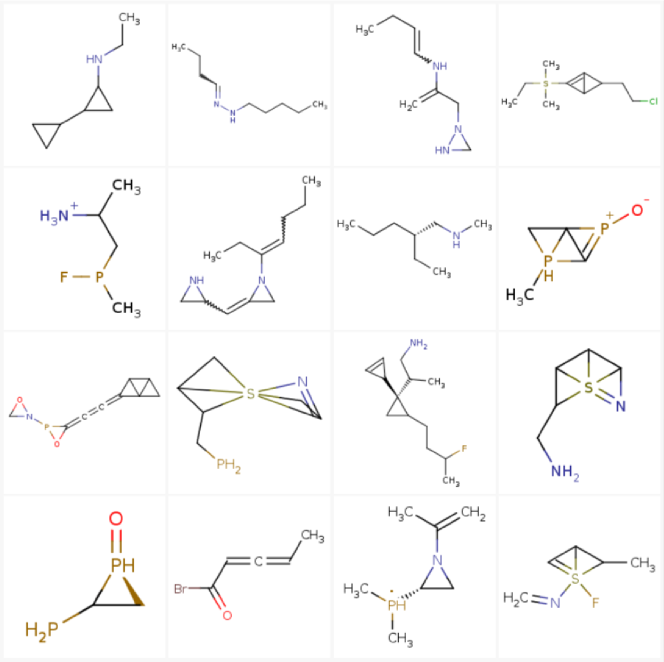
Figure 4: Examples of generated molecules.

References

- \bibcommenthead
- Arjovsky et al. (2017) Arjovsky, M., S. Chintala, and L. Bottou 2017. Wasserstein generative adversarial networks. In International conference on machine learning, pp. 214–223.
- Bernazzani et al. (2006) Bernazzani, L., C. Duce, A. Micheli, V. Mollica, A. Sperduti, A. Starita, and M.R. Tiné. 2006. Predicting physical-chemical properties of compounds from molecular structures by recursive neural networks. J. Chem. Inf. Model. 46(5): 2030–2042 .
- Bianucci et al. (2003) Bianucci, A.M., A. Micheli, A. Sperduti, and A. Starita 2003. A novel approach to qspr/qsar based on neural networks for structures. In Soft Computing Approaches in Chemistry, Volume 120 of Studies in Fuzziness and Soft Computing, pp. 265–296. Springer.
- Blaschke et al. (2018) Blaschke, T., M. Olivecrona, O. Engkvist, J. Bajorath, and H. Chen. 2018. Application of Generative Autoencoder in De Novo Molecular Design. Molecular Informatics 37(1). 10.1002/minf.201700123. arXiv:1711.07839 .
- Bradshaw et al. (2019) Bradshaw, J., B. Paige, M.J. Kusner, M.H.S. Segler, and J.M. Hernández-Lobato 2019. A model to search for synthesizable molecules. In H. M. Wallach, H. Larochelle, A. Beygelzimer, F. d’Alché-Buc, E. B. Fox, and R. Garnett (Eds.), Advances in Neural Information Processing Systems 32: Annual Conference on Neural Information Processing Systems 2019, NeurIPS 2019, December 8-14, 2019, Vancouver, BC, Canada, pp. 7935–7947.
- Bradshaw et al. (2020) Bradshaw, J., B. Paige, M.J. Kusner, M.H.S. Segler, and J.M. Hernández-Lobato 2020. Barking up the right tree: an approach to search over molecule synthesis dags. In H. Larochelle, M. Ranzato, R. Hadsell, M. Balcan, and H. Lin (Eds.), Advances in Neural Information Processing Systems 33: Annual Conference on Neural Information Processing Systems 2020, NeurIPS 2020, December 6-12, 2020, virtual.
- Brown et al. (2019) Brown, N., M. Fiscato, M.H. Segler, and A.C. Vaucher. 2019. Guacamol: benchmarking models for de novo molecular design. Journal of chemical information and modeling 59(3): 1096–1108 .
- Curtarolo et al. (2013) Curtarolo, S., G.L. Hart, M.B. Nardelli, N. Mingo, S. Sanvito, and O. Levy. 2013. The high-throughput highway to computational materials design. Nature materials 12(3): 191–201 .
- Dai et al. (2018) Dai, H., Y. Tian, B. Dai, S. Skiena, and L. Song 2018. Syntax-directed variational autoencoder for structured data. In International Conference on Learning Representations.
- De Cao and Kipf (2018) De Cao, N. and T. Kipf. 2018. MolGAN: An implicit generative model for small molecular graphs. ICML 2018 workshop on Theoretical Foundations and Applications of Dee Generative Models .
- Devi et al. (2015) Devi, R.V., S.S. Sathya, and M.S. Coumar. 2015. Evolutionary algorithms for de novo drug design–a survey. Applied Soft Computing 27: 543–552 .
- Ertl et al. (2008) Ertl, P., S. Roggo, and A. Schuffenhauer. 2008. Natural product-likeness score and its application for prioritization of compound libraries. Journal of chemical information and modeling 48(1): 68–74 .
- Gómez-Bombarelli et al. (2018) Gómez-Bombarelli, R., J.N. Wei, D. Duvenaud, J.M. Hernández-Lobato, B. Sánchez-Lengeling, D. Sheberla, J. Aguilera-Iparraguirre, T.D. Hirzel, R.P. Adams, and A. Aspuru-Guzik. 2018. Automatic chemical design using a data-driven continuous representation of molecules. ACS central science 4(2): 268–276 .
- Guimaraes et al. (2017) Guimaraes, G.L., B. Sanchez-Lengeling, C. Outeiral, P.L.C. Farias, and A. Aspuru-Guzik. 2017. Objective-reinforced generative adversarial networks (organ) for sequence generation models. arXiv preprint arXiv:1705.10843 .
- Irwin and Shoichet (2005) Irwin, J.J. and B.K. Shoichet. 2005. Zinc- a free database of commercially available compounds for virtual screening. Journal of chemical information and modeling 45(1): 177–182 .
- Jin et al. (2020) Jin, W., R. Barzilay, and T. Jaakkola 2020. Hierarchical generation of molecular graphs using structural motifs. In International Conference on Machine Learning, pp. 4839–4848. PMLR.
- Jin et al. (2018) Jin, W., R. Barzilay, and T.S. Jaakkola 2018. Junction tree variational autoencoder for molecular graph generation. In Proceedings of the International Conference on Machine Learning, pp. 2328–2337.
- Kadurin et al. (2017) Kadurin, A., A. Aliper, A. Kazennov, P. Mamoshina, Q. Vanhaelen, K. Khrabrov, and A. Zhavoronkov. 2017. The cornucopia of meaningful leads: Applying deep adversarial autoencoders for new molecule development in oncology. Oncotarget 8(7): 10883 .
- Kadurin et al. (2017) Kadurin, A., S. Nikolenko, K. Khrabrov, A. Aliper, and A. Zhavoronkov. 2017. drugan: an advanced generative adversarial autoencoder model for de novo generation of new molecules with desired molecular properties in silico. Molecular pharmaceutics 14(9): 3098–3104 .
- Kingma and Welling (2014) Kingma, D.P. and M. Welling 2014. Auto-encoding variational bayes. In Y. Bengio and Y. LeCun (Eds.), 2nd International Conference on Learning Representations, ICLR 2014, Banff, AB, Canada, April 14-16, 2014, Conference Track Proceedings.
- Knuth (1968) Knuth, D.E. 1968. Semantics of context-free languages. Mathematical systems theory 2(2): 127–145 .
- Kusner et al. (2017) Kusner, M.J., B. Paige, and J.M. Hernández-Lobato 2017. Grammar variational autoencoder. In Proceedings of International Conference on Machine Learning, pp. 1945–1954.
- Kuznetsov and Polykovskiy (2021) Kuznetsov, M. and D. Polykovskiy 2021. Molgrow: A graph normalizing flow for hierarchical molecular generation. In Thirty-Fifth AAAI Conference on Artificial Intelligence, AAAI 2021, Thirty-Third Conference on Innovative Applications of Artificial Intelligence, IAAI 2021, The Eleventh Symposium on Educational Advances in Artificial Intelligence, EAAI 2021, Virtual Event, February 2-9, 2021, pp. 8226–8234. AAAI Press.
- Liu et al. (2018) Liu, Q., M. Allamanis, M. Brockschmidt, and A.L. Gaunt 2018. Constrained graph variational autoencoders for molecule design. In Advances in Neural Information Processing Systems, pp. 7806–7815.
- Ma et al. (2018) Ma, T., J. Chen, and C. Xiao 2018. Constrained generation of semantically valid graphs via regularizing variational autoencoders. In Advances in Neural Information Processing Systems, pp. 7113–7124.
- Makhzani et al. (2015) Makhzani, A., J. Shlens, N. Jaitly, and I.J. Goodfellow. 2015. Adversarial autoencoders. CoRR abs/1511.05644. arXiv:1511.05644 .
- Oglic et al. (2018) Oglic, D., S.A. Oatley, S.J.F. Macdonald, T. Mcinally, and R. Garnett. 2018. Active Search for Computer-Aided Drug Design. Molecular Informatics 1700130: 1–16 .
- Podda et al. (2020) Podda, M., D. Bacciu, and A. Micheli 2020. A deep generative model for fragment-based molecule generation. In International Conference on Artificial Intelligence and Statistics, pp. 2240–2250. PMLR.
- Polykovskiy et al. (2018) Polykovskiy, D., A. Zhebrak, B. Sanchez-Lengeling, S. Golovanov, O. Tatanov, S. Belyaev, R. Kurbanov, A. Artamonov, V. Aladinskiy, M. Veselov, A. Kadurin, S. Nikolenko, A. Aspuru-Guzik, and A. Zhavoronkov. 2018. Molecular Sets (MOSES): A Benchmarking Platform for Molecular Generation Models. arXiv preprint .
- Polykovskiy et al. (2018) Polykovskiy, D., A. Zhebrak, D. Vetrov, Y. Ivanenkov, V. Aladinskiy, P. Mamoshina, M. Bozdaganyan, A. Aliper, A. Zhavoronkov, and A. Kadurin. 2018. Entangled conditional adversarial autoencoder for de novo drug discovery. Molecular pharmaceutics 15(10): 4398–4405 .
- Pyzer-Knapp et al. (2015) Pyzer-Knapp, E.O., C. Suh, R. Gómez-Bombarelli, J. Aguilera-Iparraguirre, and A. Aspuru-Guzik. 2015. What is high-throughput virtual screening? a perspective from organic materials discovery. Annual Review of Materials Research 45: 195–216 .
- Ramakrishnan et al. (2014) Ramakrishnan, R., P.O. Dral, M. Rupp, and O.A. von Lilienfeld. 2014. Quantum chemistry structures and properties of 134 kilo molecules. Scientific Data 1 .
- Rigoni et al. (2020a) Rigoni, D., N. Navarin, and A. Sperduti 2020a. Conditional constrained graph variational autoencoders for molecule design. In 2020 IEEE Symposium Series on Computational Intelligence (SSCI), pp. 729–736. IEEE.
- Rigoni et al. (2020b) Rigoni, D., N. Navarin, and A. Sperduti. 2020b. A systematic assessment of deep learning models for molecule generation. 2020 European Symposium on Artificial Neural Networks (ESANN) .
- Ruddigkeit et al. (2012) Ruddigkeit, L., R. Van Deursen, L.C. Blum, and J.L. Reymond. 2012. Enumeration of 166 billion organic small molecules in the chemical universe database gdb-17. Journal of chemical information and modeling 52(11): 2864–2875 .
- Samanta et al. (2019) Samanta, B., A. De, G. Jana, P.K. Chattaraj, N. Ganguly, and M.G. Rodriguez 2019. Nevae: A deep generative model for molecular graphs. In The Thirty-Third AAAI Conference on Artificial Intelligence, AAAI 2019, pp. 1110–1117.
- Schlichtkrull et al. (2018) Schlichtkrull, M., T.N. Kipf, P. Bloem, R. Van Den Berg, I. Titov, and M. Welling 2018. Modeling relational data with graph convolutional networks. In European semantic web conference, pp. 593–607. Springer.
- Segler et al. (2018) Segler, M.H., T. Kogej, C. Tyrchan, and M.P. Waller. 2018. Generating focused molecule libraries for drug discovery with recurrent neural networks. ACS central science 4(1): 120–131 .
- Shi et al. (2019) Shi, C., M. Xu, Z. Zhu, W. Zhang, M. Zhang, and J. Tang 2019. Graphaf: a flow-based autoregressive model for molecular graph generation. In International Conference on Learning Representations.
- Shi et al. (2020) Shi, C., M. Xu, Z. Zhu, W. Zhang, M. Zhang, and J. Tang 2020. Graphaf: a flow-based autoregressive model for molecular graph generation. In 8th International Conference on Learning Representations, ICLR 2020, Addis Ababa, Ethiopia, April 26-30, 2020. OpenReview.net.
- Weininger (1988) Weininger, D. 1988. Smiles, a chemical language and information system. 1. introduction to methodology and encoding rules. Journal of chemical information and computer sciences 28(1): 31–36 .
- Weininger (1990) Weininger, D. 1990. Smiles. 3. depict. graphical depiction of chemical structures. Journal of chemical information and computer sciences 30(3): 237–243 .
- Weininger et al. (1989) Weininger, D., A. Weininger, and J.L. Weininger. 1989. Smiles. 2. algorithm for generation of unique smiles notation. Journal of chemical information and computer sciences 29(2): 97–101 .
- Xu et al. (2019) Xu, K., W. Hu, J. Leskovec, and S. Jegelka 2019. How powerful are graph neural networks? In 7th International Conference on Learning Representations, ICLR 2019, New Orleans, LA, USA, May 6-9, 2019. OpenReview.net.
- Zang and Wang (2020) Zang, C. and F. Wang 2020. Moflow: An invertible flow model for generating molecular graphs. In R. Gupta, Y. Liu, J. Tang, and B. A. Prakash (Eds.), KDD ’20: The 26th ACM SIGKDD Conference on Knowledge Discovery and Data Mining, Virtual Event, CA, USA, August 23-27, 2020, pp. 617–626. ACM.