EUV fine structure and variability associated with coronal rain revealed by Solar Orbiter/EUI HRI_EUVand SPICE

Abstract

Context. Coronal rain is the most dramatic cooling phenomenon of the solar corona. Recent observations in the visible and UV spectrum have shown that coronal rain is a pervasive phenomenon in active regions. Its strong link with coronal heating through the Thermal Non-Equilibrium (TNE) - Thermal Instability (TI) scenario, makes it an essential diagnostic tool for the heating properties. Another puzzling feature of the solar corona, besides the heating, is its filamentary structure and variability, particularly in the EUV.

Aims. We aim to identify observable features of the TNE-TI scenario underlying coronal rain at small and large spatial scales, to understand the role it plays in the solar corona.

Methods. We use EUV datasets at unprecedented spatial resolution of $\approx 240\leavevmode\nobreak\$km from the High Resolution Imager (HRI) in the EUV (HRI_EUV) of the Extreme Ultraviolet Imager (EUI) and SPICE on board Solar Orbiter from the spring 2022 perihelion.

Results. EUV absorption features produced by coronal rain are detected at scales as small as 260 km. As the rain falls, heating and compression is produced immediately downstream, leading to a small EUV brightening accompanying the fall and producing a ‘fireball’ phenomenon in the solar corona. Just prior to impact, a flash-like EUV brightening downstream of the rain, lasting a few minutes is observed for the fastest events. For the first time, we detect the atmospheric response to the rain’s impact on the chromosphere and consists of upward propagating rebound shocks and flows partly reheating the loop. The observed widths of the rain clumps are $500\pm 200\leavevmode\nobreak\$km. They exhibit a broad velocity distribution of $10-150\leavevmode\nobreak\$km s^-1, peaking below 50 km s^-1. Coronal strands of similar widths are observed along the same loops co-spatial with cool filamentary structure seen with SPICE, which we interpret as the Condensation Corona Transition Region. Matching with the expected cooling, prior to the rain appearance sequential loop brightenings are detected in gradually cooler lines from corona to chromospheric temperatures. Despite the large rain showers, most cannot be detected in AIA 171 in quadrature, indicating that line-of-sight effects play a major role in coronal rain visibility. Still, AIA 304 and SPICE observations reveal that only a small fraction of the rain can be captured by HRI_EUV.

Conclusions. Coronal rain generates EUV structure and variability over a wide range of scales, from coronal loop to the smallest resolvable scales. This establishes the major role that TNE-TI plays in the observed EUV morphology and variability of the corona.

1 Introduction

The solar corona is mysteriously heated to millions of degrees by yet unclear mechanisms of magnetic energy conversion and transport in plasmas. Coronal loops, the building blocks of the inner solar corona, constitute the prime target for the coronal heating investigation, due to their visibility above the diffuse background. Many of their properties remain a puzzle, such as their lifetimes (EUV variation), and morphologies (in particular their sub-structure) (Reale, 2010; Klimchuk, 2015; Viall et al., 2021). For instance, a long-standing puzzle of the corona is the observed filamentary / strand-like structure of loops (as opposed to being diffused) and their high variability, particularly in the upper transition region (TR) spectral lines (Kjeldseth-Moe & Brekke, 1998; Ugarte-Urra et al., 2009; Hinode Review Team et al., 2019). The filamentary structure is linked with the loop sub-structure, with the concept of coronal strands introduced and usually assumed to be part of a larger entity (or coronal loop ‘bundle’). This multi-stranded vs. monolithic structure has been a long-standing debate in the solar community. Its importance stems from its strong link with the fundamental scales in which the heating operates in the solar atmosphere, either directly associated with the scales at granular level, where most of the energy originates (Martínez-Sykora et al., 2018), or indirectly, e.g. by modifying how MHD waves propagate and dissipate in inhomogeneous plasmas (Van Doorsselaere et al., 2014, 2020).

Prior to the Solar Orbiter launch (Müller et al., 2020), Hi-C (1st and 2nd flights Kobayashi et al., 2014; Rachmeler et al., 2019), provided the highest spatial resolution observations in the EUV, namely in the Fe xii 193 Å  line forming at $\approx 1.5\times 10^{6}$ K (1st flight) and in the Fe ix 172 Å  line forming at $\approx 10^{5.9}$ K (2nd flight). These observations indicate coronal strand widths on the order of a few hundred km (Peter et al., 2013; Brooks et al., 2013; Aschwanden & Peter, 2017; Williams et al., 2020). On the other hand, such sub-structure does not appear to be present for all coronal loops and across different temperature regimes, as the above reports show. Sub-structure, such as coronal strands, may appear during the evolution of the loops, particularly their cooling, and thus may be linked to specific aspects of how the cooling happens.

Coronal rain is the most dramatic display of cooling in the solar corona. It corresponds to cool ($10^{3}-10^{5}$ K) and dense ($10^{10}-10^{13}$ cm ^-3) plasma clumps appearing over a timescale of minutes in chromospheric and TR spectral lines in the solar corona, that preferentially fall towards the solar surface along coronal loops (Kawaguchi, 1970; Leroy, 1972; Habbal et al., 1985; Foukal, 1978; Wiik et al., 1996; Schrijver, 2001; De Groof et al., 2004, 2005). Coronal rain is closely related to prominences (Vial & Engvold, 2015), but high-resolution observations over the last decade with Hinode (Kosugi et al., 2007; Antolin & Shibata, 2010; Hinode Review Team et al., 2019), the Swedish 1-m Solar Telescope (SST; Scharmer et al., 2003; Antolin & Rouppe van der Voort, 2012), the Goode Solar Telescope (GST; Goode et al., 2003; Ahn et al., 2014; Jing et al., 2016), the Solar Dynamics Observatory (SDO; Pesnell et al., 2012; Vashalomidze et al., 2015) and the Interface Region Imaging Spectrograph (IRIS; De Pontieu et al., 2014; Antolin et al., 2015; Schad, 2017; De Pontieu et al., 2021) have shown that coronal rain presents unique features in terms of its morphology and kinematics. At the smallest scales, coronal rain appears to be composed of clumps, which seem to also constitute the coolest and densest part. The widths (in the direction transverse to the flow) can be as low as 120 km (Jing et al., 2016) but generally are a few hundred km in H$\alpha$ (Antolin & Rouppe van der Voort, 2012) to $\approx 500-600\leavevmode\nobreak\$km in TR lines (Antolin et al., 2015), with little variation other than that expected by spatial resolution. On the other hand, they can extend greatly longitudinally (along the flow), with lengths about an order of magnitude or more. Recently, Sahin et al. (2023) studied large-scale coronal rain over an active region (AR) with IRIS in chromospheric and TR lines, finding little variation in its morphological and dynamical properties over several hours and across the AR. The observed coronal rain strands appear to have very similar widths to the coronal strands observed by Hi-C, described above, which may either directly reflect a fundamental heating scale (Jing et al., 2016; Antolin & Froment, 2022) or be associated with the cooling, as explained below.

One of the most interesting aspects of coronal rain is that the clumps occur in tandem across a relatively large cross-section across the magnetic field (of a few Mm in width). This synchronicity and shared trajectory of clumps has led to the concept of rain shower, i.e. a larger-structure composed of coronal rain clumps (Antolin & Rouppe van der Voort, 2012). Şahin & Antolin (2022) have shown that rain showers match well with cooling coronal loops observed in EUV, thereby helping to identify these in the large superposition (leading to line-of-sight confusion) of the optically thin solar corona (what Malanushenko et al., 2022, refer to as ‘coronal veil’).

There are currently 3 different kinds of coronal rain. The most commonly observed kind is known as ‘quiescent’, and occurs preferentially in AR coronal loops. This kind does not require any specific magnetic topology (other than a loop-forming bi-polar structure). The second kind is linked to solar flares and is known as ‘flare-driven’ coronal rain. It corresponds to the cool chromospheric loops (sometimes known as H$\alpha$ loops) appearing at the end of the gradual phase. The last kind is known as prominence-coronal rain hybrids, and involves a complex magnetic field with null-point topology at the top of loop arcades. A review of each can be found in Antolin & Froment (2022). This work concerns the first kind, that is, the quiescent coronal rain of ARs. This kind is the most actively studied probably because of its strong link with coronal heating.

Numerical work since the 90s have shown that complex magnetic topologies such as magnetic dips are not necessary for the generation of cool and dense, prominence-like structures in loops (Antiochos & Klimchuk, 1991; Antiochos et al., 1999; Karpen et al., 2001). Although we do not know what exactly the agents of coronal heating are (e.g. MHD waves or stress-induced magnetic reconnection), the generated spatial and temporal distribution of the magnetic energy along loops has unique consequences on the evolution of coronal loops, specifically on how they cool down. When the heating is strongly stratified (also known as ‘footpoint concentrated’), even if constant over time, the loop is often unable to reach thermal equilibrium and enters a state of thermal non-equilibrium (TNE). Its thermodynamic evolution undergoes cycles of heating and cooling, generally referred as TNE cycles, also known as evaporation-condensation cycles (Kuin & Martens, 1982; Mok et al., 1990; Reale et al., 1996; Müller et al., 2003; Mendoza-Briceño et al., 2005; Susino et al., 2010; Luna et al., 2012). This is true as long as the repetition frequency of the stratified heating events is faster than the radiative cooling time of the loop (Johnston et al., 2019). Klimchuk & Luna (2019) have quantified some of the requirements needed for TNE, and found that a volumetric heating ratio between apex and footpoint below 0.3 and a heating asymmetry between both footpoints under 3 ensures TNE.

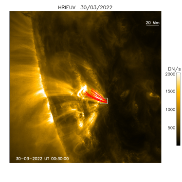
(a)

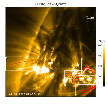
(b)

Figure 1: Full FOV of HRI_EUV for the 2022 March 30 (left) and April 1 (right) datasets analysed in this work. The inner white rectangles show sub-FOVs shown in later figures. The solid red curves denote the trajectories of some of the observed coronal rain clumps.

In a nutshell, with a strongly stratified heating, the loop apex relies on thermal conduction for its heating. However, this spatial distribution leads to an essentially flat temperature profile along the loop length, or even a temperature dip at the apex, thus making conduction inefficient. Furthermore, the footpoint heating is very efficient at injecting material upwards (through chromospheric ablation / evaporation), making the loop overdense relative to the RTV scaling law (Rosner et al., 1978). The apex ends up having a thermal imbalance, which results in a runaway or catastrophic cooling due to the higher efficiency for plasmas at radiating their energy away at lower temperatures (in the TR - corona temperature range). While the heating can be very rapid (with the loop essentially empty) and therefore very hard to observe, the cooling progresses over a timescale of tens of minutes to hours, depending on the loop conditions. These long cooling times can lead to very long loop lifetimes (Lionello et al., 2016). The loop eventually evacuates and the cycle restarts if the heating conditions do not change, hence leading to cycles of heating and cooling. During the initial stages of the cooling, and when the cooling time is long enough relative to the cadence of the observations, the loop is expected to sequentially appear in cooler coronal passbands with specific non-zero timelags (Kamio et al., 2011; Viall & Klimchuk, 2012; Viall et al., 2021). The cyclic pattern can lead to highly periodic EUV intensity pulsations on the order of hours, recently detected with EIT (Auchère et al., 2014) and the Atmospheric Imaging Assembly (AIA; Lemen et al., 2012; Froment et al., 2015), indicating a heating function that is stable over days (and up to a week). At the end of the cooling part of the TNE cycle accelerated cooling is observed and coronal rain appears, which can therefore also occur periodically (Auchère et al., 2018; Froment et al., 2020). This acceleration in the cooling rate and also the spatial and temporal character of coronal rain have been interpreted as a product of thermal instability (TI), but a debate exists in the community (Klimchuk, 2019; Antolin, 2020). The essential role that TI may play in the observed coronal rain phenomena (and probably the long-period intensity pulsations as well), has led to the cycles being known as TNE-TI cycles (Antolin & Froment, 2022).

Thermal instability is a fundamental MHD process (Parker, 1953; Field, 1965; Waters & Proga, 2019; Claes, N. & Keppens, R., 2019). Besides coronal rain, it has been invoked to explain phenomena from the short laboratory scales (Lipschultz, 1987; Stacey, 1996), to very large intracluster medium scales (White & Rees, 1978; Cavagnolo et al., 2008; Sharma, 2013). In the context of the solar corona, thermal instability is less straightforward to apply because the corona is very dynamic and is out of hydrostatic equilibrium (Aschwanden et al., 2001). Nonetheless, various analytic studies have argued that given the long timescales of TNE cycles, TI theory still holds, given the local and short timescale characteristics of its occurrence (Claes & Keppens, 2021). Antolin & Rouppe van der Voort (2012) and Antolin et al. (2015) have argued that TI may act as a synchronising mechanism for catastrophic cooling to occur simultaneously across a loop in TNE, thereby providing an explanation for rain showers (see also Froment et al., 2020; Antolin, 2020). Şahin & Antolin (2022) have used this link to unlock a way to estimate the TNE volume over an AR. By calculating the number of rain showers and their properties, they have estimated that at least 50% of the AR is subject to TNE.

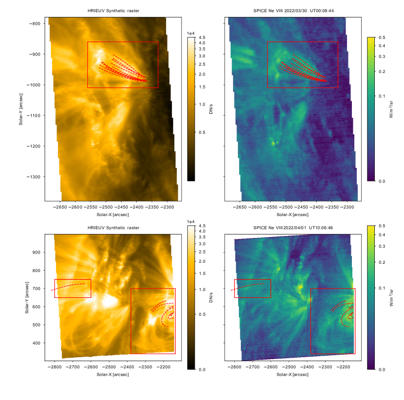
Figure 2: Co-aligned HRI_EUV (left) and SPICE (right) full FOV for March 30 (top) and April 1 (bottom). The SPICE images correspond to a 96- and 160-step rasters for March 30 and April 1, respectively, and show the total intensity over the Ne VIII line. The corresponding HRI_EUV images are synthetic rasters that match the time and space distribution of data acquisition with SPICE. A spatial binning has been applied to HRI_EUV to match the platescale of SPICE. The red rectangles correspond to regions of interest (ROI) in each FOV with overlaid rain paths in red identified with HRI_EUV. The ROI on March 30 is shown in Figure 5. The ROIs on April 1 to the West and East are shown in Figures 13 and 17, respectively. See text for further details.

2.5-D radiative MHD simulations by Antolin et al. (2022) have shown that the TI-driven catastrophic cooling leads to the formation of cool and dense cores at the head of the rain emitting in chromospheric lines, surrounded by thin but strongly emitting shells in TR lines that elongate in the wake of the rain, in what is known as the Condensation Corona Transition Region (CCTR). These structures are seen clearly in the Si IV 1402 line observed by IRIS (forming at $\approx 10^{4.8}\leavevmode\nobreak\$K), and the Fe xii 171 line observed by AIA 171 (forming at $\approx 10^{5.8}$ K), and could therefore explain the filamentary/stranded morphology and dynamic nature of the corona seen in these lines (Ugarte-Urra et al., 2009), as well as the common widths between coronal rain strands and coronal EUV sub-structure. High-resolution observations in the EUV are needed to confirm this hypothesis. Furthermore, Antolin et al. (2022) have shown that TI produces a local enhancement of the magnetic field strength, due to the gas pressure loss during TI and frozen-in conditions. Due to the compression ahead of the rain (downstream) as it falls, a strong UV and EUV enhancement is obtained over the last few Mm prior to impact with the chromosphere. Furthermore, a strong rebound shock and upward flow is obtained from the impact, propagating at different speeds (corresponding to the tube speed and flow). These features have remained elusive in observations until now.

Solar Orbiter was launched in early 2020 on a highly elliptical orbit around the Sun. By now, it has concluded two science close perihelia in its nominal mission phase, where the distance to the Sun was less than 0.32 au. In this work we analyse data from one of the two High Resolution Imagers (HRI) of the Extreme Ultraviolet Imager (EUI) telescopes on board Solar Orbiter (Rochus et al., 2020), corresponding to the first close perihelion, which happened between March and April 2022 (Berghmans et al., 2023). The HRI_EUV is an EUV imaging instrument in the 174 Å  passband, which is dominated by the Fe ix (at 171.1 Å ) and Fe x (at 174.5 Å  and 177.2 Å ) emission forming at $\approx 10^{6}\leavevmode\nobreak\$K (Chen et al., 2021). The importance of the high resolution achieved by this instrument was already evident in HRI_EUV data from May 2020, when the spacecraft was at 0.556 au, which revealed small EUV brightenings at spatial and temporal resolutions that could be barely detected by SDO/AIA observations (known as ‘campfires’; Berghmans et al., 2021).

EUI also includes a high-resolution imager HRI_Lya, whose bandpass is centered at 121.6 nm and is dominated by the Lyman-$\alpha$ line of hydrogen. We do not useHRI_Lya in this work due to the degradation issues the telescope suffered during the perihelion approach (see Berghmans et al., 2023, for details).

In this work we analyse HRI_EUV data and identify several coronal rain events at unprecedented spatial resolution of $\approx 240$ km in the EUV that allow us to clearly identify the EUV variability and morphology associated with coronal rain. The paper is organised as follows. The HRI_EUV observations are presented in Section 2. The methods are presented in Section 3. Results can be found in Section 4, and discussion and conclusions in Section 5.

2 Observations

The observations analysed in this work belong to the first perihelion passage of Solar Orbiter in March and April 2022. Specifically, we analyse two datasets of HRI_EUV at 174 Å, one of NOAA 12974 on 2022 March 30, and the other of ARs NOAA 12975 and 12796 on 2022 April 1, both on-disk (Mampaey et al., 2022). At this time, Solar Orbiter was near quadrature with Earth (with separation angles between Solar Orbiter and the Sun-Earth line of $91.88^{\circ}$ and $102.02^{\circ}$ for March 30 and April 1, respectively).

On March 30 and April 1, Solar Orbiter was at 0.33 au and 0.34 au, respectively. With an HRI_EUV plate scale of 0.492″, the spatial resolution of these observations is estimated to be close to the Nyquist limit of $2\times 0.492\arcsec$ (Berghmans et al., 2023), corresponding to 237 km and 247 km, approximately. HRI images have $2048\times 2048$ pixels, leading to a $17^{\prime}\times 17^{\prime}$ field-of-view (FOV). The full FOV for each date can be seen in Figure 1. The observations on March 30 and April 1 are part of the R_BOTH_HRES_HCAD_Nanoflares and R_SMALL_MRES_MCAD_AR-Long-Term SOOPs (Zouganelis et al., 2020), respectively, which operated the HRI_EUV camera at a cadence of 3 s over a duration of 45 min (UT 00:03 – 00:48) on March 30, and at a cadence of 10 s over a duration of $\approx 75\leavevmode\nobreak\$min (UT 09:19 – 10:34) on April 1.

EUI is equipped with software controlled onboard calibration electronics to correct the images pixel-wise for offset and flat field before compression. The images are then prepped with the euiprep routine to level 2, which reduces the jitter and pointing error. However, significant jitter still remains that needs to be removed. To this end, we apply a cross-correlation technique to align the images as described in Chitta et al. (2022).

For better visualisation of the fine structure in the HRI_EUV images, we have applied the wavelets-optimised whitening (WOW) enhancement technique described in Auchère et al. (2023). This method works by equalizing the variance at all scales and locations in the image, thereby reducing the large scale gradients and conversely enhancing the small scale structures.

We have also checked HRI_Lya for the presence of rain in the Lyman-$\alpha$ line. However, none could be detected probably due to the problem affecting the resolution of the instrument, as discussed in Berghmans et al. (2023).

Solar Orbiter also carries the Spectral Imaging of the Coronal Environement (SPICE, SPICE Consortium et al., 2020), as part of the remote sensing payload. For March 30, the SPICE data analyzed (data release 3.0), is the 96-step raster starting at 00:00:32 UTC with a field of view of $384^{\prime\prime}\times 914^{\prime\prime}$. It has a duration of 16 min 24 s and an exposure time of 10 s. The selected slit is 4″wide, while the data spatial pixel size is 1.098″along the slit. The temperature coverage of the spectral windows was from the chromosphere to the corona through the observation of the following spectral lines: H I Ly$\beta$ 1025.72 Å (Log $T_{e}$ = 4.0 K); C III 977.03 Å (Log $T_{e}$ = 4.8 K); S V 786.47 Å (log $T_{e}$ = 5.2 K); O IV 787.72 Å (log $T_{e}$ = 5.2 K); O VI 1031.93 Å (log $T_{e}$ = 5.5 K); Ne VIII 770.42 Å (log $T_{e}$ = 5.8 K ); Mg IX 706.02 Å (log $T_{e}$ = 6.0 K). For April 1st, we analysed five 160-step rasters which use the 4^′′ slit each producing a field of view of $640^{\prime\prime}\times 911^{\prime\prime}$. They run from 09:15:36 to 10:15:37 UTC. The rasters duration is 14 min with the exposure time of 5 s. The spectral windows of April 1^st study covered similar lines as the March 30 raster, with the exception of the S V and O IV lines. These two lines were replaced by N IV 765.15 Å (Log $T_{e}$ = 5.2 K). For both datasets we used L2 data which are original data corrected for dark current, flat-field, geometrical distortion. An additional step in the data processing was the application of the radiometric calibration.

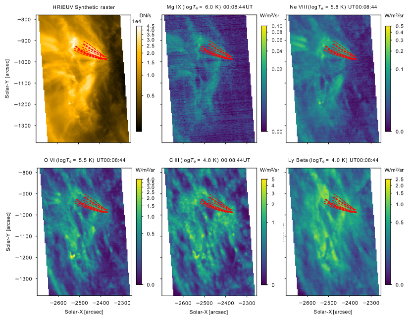
Figure 25: SPICE multi-wavelength full FOV on March 30. The SPICE FOV is the same as that shown in Figure 2 (top). The HRI_EUV panel corresponds to a synthetic raster matching the time of the SPICE raster (see text for details) including spatial binning to match the SPICE platescale. Each SPICE panel shows the total intensity over the indicated spectral line, together with its temperature of maximum formation. The overlaid red curves denote the rain paths seen with HRI_EUV (see Figure 4).

The pointing information in SPICE L2 headers is not accurate and the SPICE rasters need to be co-aligned with the HRI_EUV sequence. We started by binning the HRI_EUV images to the same pixel size of SPICE. We then built a HRI_EUV synthetic raster by selecting, from the HRI_EUV time sequence, the image closest in time to each SPICE exposure making the raster. For each SPICE exposure, the SPICE pixel positions along the slit make an irregular grid in Helioprojective coordinates. The HRI_EUV image closest in time to this exposure is reprojected into this grid. We then made SPICE images in Ne VIII intensity by spectrally summing over the 32 pixels window. The Ne VIII and HRI_EUV images are, in fact, comparable in terms of plasma temperature coverage. Finally, the SPICE images are co-aligned with the HRI_EUV synthetic raster using a cross-correlation technique. The SPICE FOV for March 30 and April 1 in the Ne VIII line co-aligned with HRI_EUV can be seen in Figure 2. Snapshots of each FOV in all the other spectral lines are shown in Figure 25 for March 30 and Figure 24 for April 1.

In addition to EUI images we also briefly analyse images from the Atmospheric Imaging Assembly (AIA; Lemen et al., 2012) on board the Solar Dynamics Observatory (SDO; Pesnell et al., 2012) to locate, if possible, the coronal rain events observed with HRI_EUV. The AIA data correspond to level 2 data, processed through the standard SolarSoft packages. Since strict AIA-EUI co-alignment at a pixel scale is not needed for our purpose (we do not need to identify specific rain trajectories across different viewpoints), we rely on co-alignment using header information through the JHelioviewer software (Müller et al., 2009), which is sufficient to identify the large-scale structure common to both FOVs (such as loops, rain showers, prominences etc.).

3 Methodology

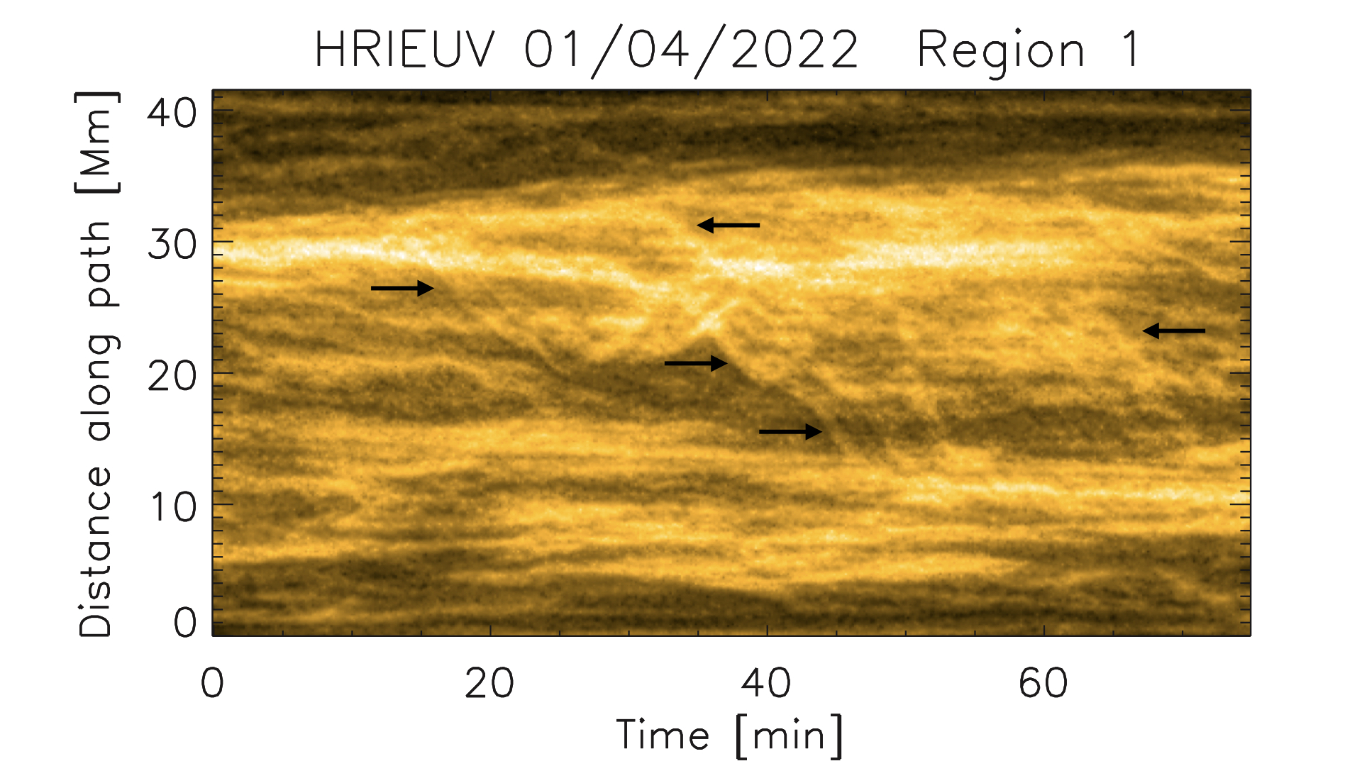
Figure 3: Time-distance diagram along the white dashed curve in Figure 1 (right panel) for the April 1 HRI_EUV observation, with distance ‘0’ corresponding to the western end of the curve. The curve crosses a loop bundle at the apex, which is seen to undergo a large-scale reconfiguration (radially inward corresponding to shrinkage), as pointed by the arrows. This time-distance diagram is made from images that have been processed with the wavelet-optimised whitening enhancement technique of Auchère et al. (2023).

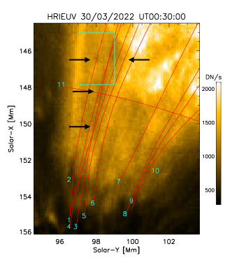
Figure 4: Close-up on the footpoint of the loop bundle where coronal rain is seen on March 30. The FOV corresponds to the white rectangle shown in Fig. 1 (left), rotated by 90^∘ so that the loop is orientated with the height of the page. The red and labelled curves vertically oriented denote several rain clump trajectories. The black arrows point to some of the clumps. The image corresponds to the average over 3 consecutive frames. The cyan rectangle in the figure corresponds to the FOV shown in Figure 7. Path 11 is a transverse cut across the loop bundle. The accompanying animation runs from UT 00:23 to UT 00:37 and shows several coronal rain clumps in absorption falling towards the chromosphere (dark structure at bottom). Note the strong EUV variation associated with this event. The images composoing the movie are processed with the wavelet-optimized whitening enhancement technique of Auchère et al. (2023). The movie first runs without and then with the rain paths overlaid.

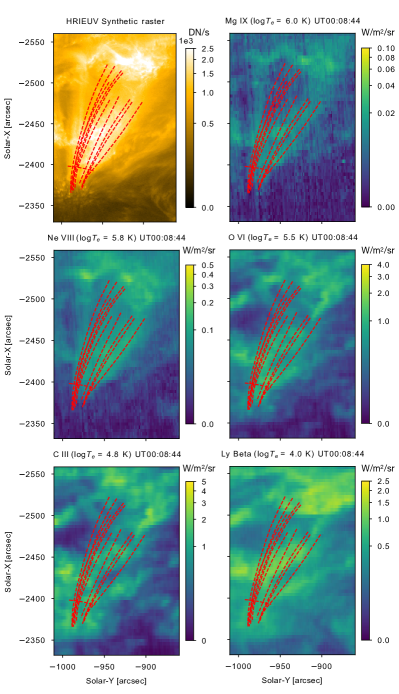
Figure 5: SPICE multi-wavelength view on the loop bundle with rain seen on March 30. The FOV corresponds to the red rectangle shown in Figure 2 (top) and the overlaid red curves mostly denote the rain paths seen with HRI_EUV (see Figure 4). The HRI_EUV panel corresponds to a synthetic raster matching the time of the SPICE raster (see text for details) but preserving the HRI_EUV spatial resolution. Each SPICE panel shows the total intensity over a spectral line indicated in the subtitle, together with its temperature of maximum formation.

Coronal rain clumps and showers can be seen with a sharp eye without any image enhancement technique such as ‘WOW’, but certainly become more discernible in the processed images. To analyse the morphology and dynamics of several of these events we start by tracking several rain clumps manually in the image sequences, with the help of CRISPEX (CRisp SPectral EXplorer), a widget-based tool programmed in the Interactive Data Language (IDL), which enables the easy browsing of the data, the determination of loop paths, extraction, and further analysis of space-time diagrams (Vissers & Rouppe van der Voort, 2012).

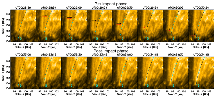
Figure 6: Sequence of 8 snapshots separated by 15 s showing the pre- (top) and post-impact (bottom) phases of a coronal rain shower from the event of March 30. The black arrows on the top panels show the head of a rain clump as it falls (note the bright tip indicated by red arrows, followed by a dark elongated structure). For reference, path 5 is shown in the Figure with a cyan-black dashed curve (same labelling as in Fig. 4). The lower panel shows a bright upward propagating feature that we interpret as a combination of a rebound shock and flow produced by the impact of the rain shower. These images have been processed with the wavelet-optimized whitening enhancement technique of Auchère et al. (2023).

The determination of projected velocities in the plane-of-the-sky (POS) is done by calculating slopes in resulting rain clump tracks in the time-distance diagrams obtained from CRISPEX. These tracks define $(x,y,t)$ positions of the rain. The errors incurred in this process depend on the length of the tracks in the time-distance diagrams. By varying slightly the spatial and temporal end points of the tracks it is possible to estimate the errors in each calculation. The availability of AIA in quadrature would allow to estimate the total speed of a rain event through 3D stereoscopy. However, this is beyond the scope of the present manuscript.

No rain is detected in the time-distance diagrams (through dark or bright propagating features) without prior check with the image sequences. This is necessary since several effects (such as lateral motions of loops) can produce apparent dark or bright propagating features in time-distance diagrams.

Regarding the morphology of the rain, we are primarily interested in the observed widths. For this purpose, we apply the same semi-automatic routine as in previous work (for more details see Antolin et al., 2015). For a given clump path and a given track in the time-distance diagram corresponding to this path, the routine takes a cut perpendicular to the trajectory at every $(x,y,t)$ location defined by the track and fits a single Gaussian over the interpolated profile. The Full-Width at Half-Maximum (FWHM) is then taken as the width of the clump at that location. Several checks are performed to reduce errors in the fitting. We first calculate the average intensity profile of a feature for the time range in which it is seen (as defined by a slope in the time-distance diagram) and require a difference of at least 100 DN s^-1 between its intensity (which can be in emission or absorption) and the background (which is also calculated over the same path but at times without rain, immediately before or after the rain episode). We then require the contrast between the feature’s average intensity and the background to be at least 10 %. Lastly, we also require that the Gaussian fit of the rain feature is good enough. The latter is ensured by requiring that the $\sigma-$error resulting from the fit is below 0.4 and that the total of the residuals fromt he fit is low, that is $\sum|I_{x,y}(x_{\perp},y_{\perp},t)-f(x_{\perp},y_{\perp},t)|<0.75$, where $(x_{\perp},y_{\perp})$ denotes the transverse cut to the path at point $(x,y)$, $I$ is the intensity along this cut, and $f$ denotes the Gaussian fit to $I$. Visual inspection of the fittings indicate that these values ensure an accurate calculation of the rain width while avoiding artefacts due to cosmic rays or other features. The width of a clump corresponds to the average over all measurements performed for the track in the time-distance diagram corresponding to that clump. A measure of the error in the width calculation is given by the standard deviation over all the measurements for a given track.

4 Results

4.1 Coronal loop bundles

We analyse several coronal rain events observed with HRI_EUV. On March 30, the event occurs in a coronal loop bundle belonging to AR NOAA 12974 in the southern hemisphere, which is on-disk but near the limb as seen in Figure 1 (left panel). The rain is seen to fall onto the leading polarity, onto a region with abundance of dark jet-like structures fanning outwards. No sunspot is seen in the vicinity, suggesting that this corresponds to a decaying AR. Several rain clumps were followed, whose trajectories can be seen in the figure.

On April 1, HRI_EUV observed a wide region of activity composed of 2 ARs, NOAA 12975 and 12976, in the northern hemisphere, also not far from the limb as seen in Figure 1 (right panel). Coronal rain is seen much more pervasively compared to the other HRI_EUV observation. In particular, we analysed four different regions, labelled in the panel, where several coronal rain events can be seen, as indicated in the figure.

Region 1 focuses on the West footpoint of a very large coronal loop bundle that is seen to undergo a wide-scale reconfiguration. Some of this reconfiguration is also associated with a bundle of loops that are rooted closer to the lower-right corner of box-2 in the right panel of Figure1. To see this more clearly we take a transverse cut at the apex of the loop bundle, as shown by the dashed curve in the right panel, and plot the time-distance diagram in Figure 3 (distance ‘0’ in the diagram denotes the western end of the dashed curve, as seen in Figure 1). In the diagram we indicate with arrows several instances of large-scale motions of individual coronal strands directed radially inwards, suggesting a shrinkage. This process is also accompanied by large-amplitude transverse oscillations that can also be identified in the figure. At the same time, large amounts of coronal rain are observed to fall along the leg captured by Region 1.

Region 2 on April 1 focuses on a region with different polarity compared to Region 1, where the other footpoint of the loop bundle appears to be rooted. Region 2 shows stronger activity (pores, moss, light-walls and jets) and a more complex magnetic topology as discussed in the accompanying paper (Berghmans et al., 2023). Between regions 1 and 2, a highly twisted filament is seen, whose eruption was observed by EUI and SPICE on the following day, and is discussed in (Berghmans et al., 2023).

Region 3 on April 1 is located at the North-West of the AR. A different bundle of loops is seen, with footpoints close to those in Region 2, and therefore also in a high-activity region.

Region 4 on April 1 is located on the East limb and captures part of a long loop that is rooted in the trailing AR (NOAA 12976).

4.2 March 30 loop bundle as seen with SPICE

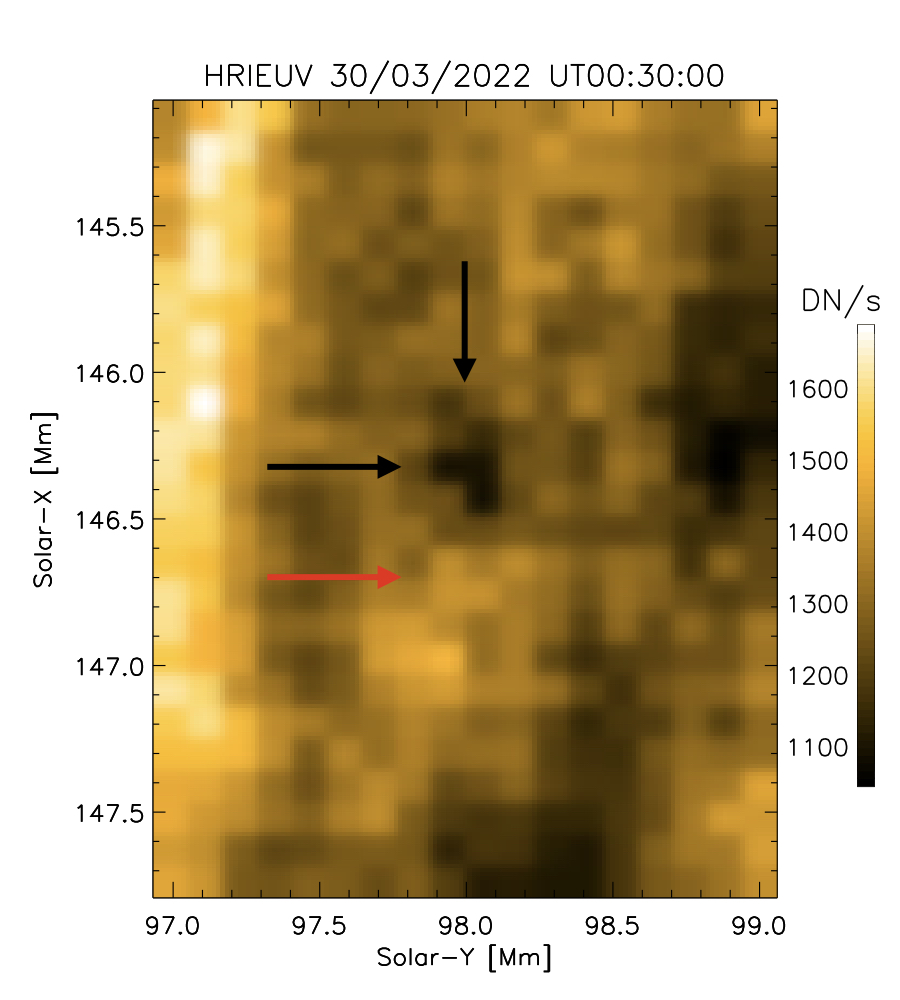
Figure 7: Close-up of the sub-FOV indicated by the white rectangle in Figure 4. The dark feature indicated by the arrows corresponds to the EUV absorption produced by a rain clump. We interpret the bright feature below (downstream of) the rain clump indicated by the red arrow as compression and heating produced by the rain clump as it falls.

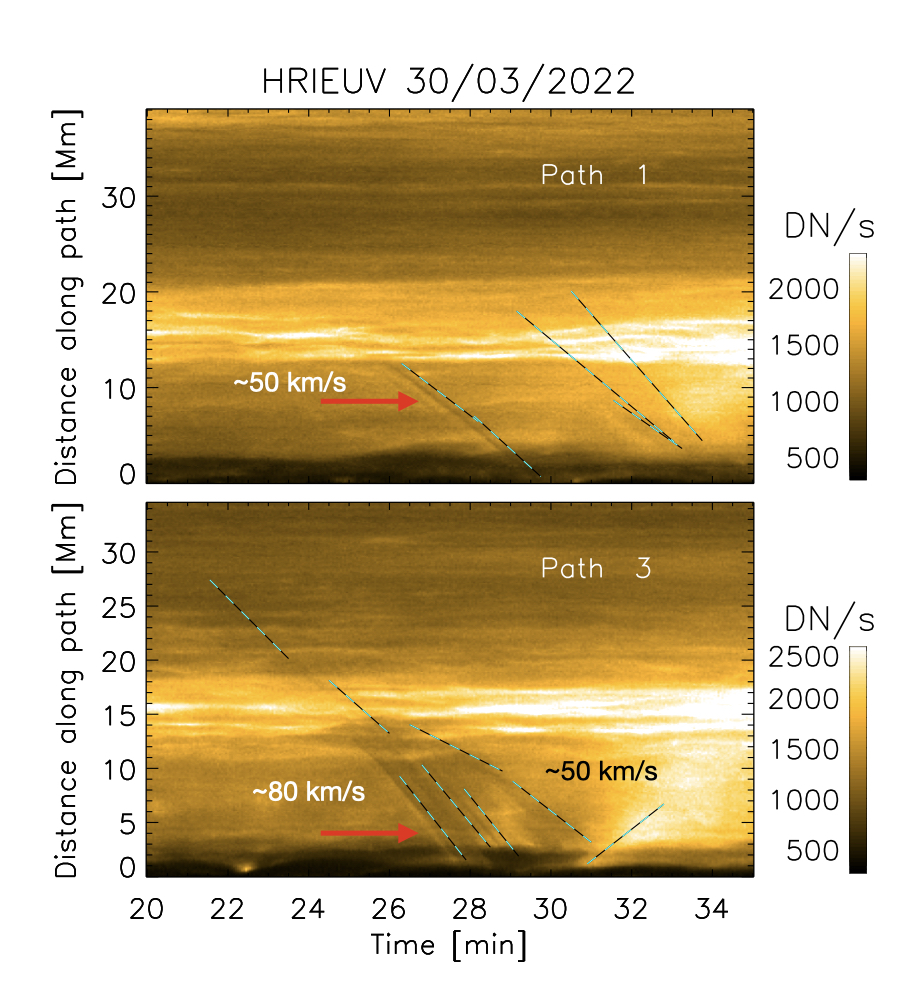
Figure 8: Time-distance diagrams along paths 1 and 3 indicated in Figure 4. Distance increases with height along the paths. The dark tracks traced by cyan-black dashed lines correspond to EUV absorption from falling rain clumps. The dashed lines are offset by a fraction of a minute in order to better see the rain features. An estimate of the projected velocity is given for the closest slope to each value. Note the bright tracks indicated by the red arrows immediately beneath the first dark tracks in each diagram. We interpret this feature as compression and heating from the clump. We interpret the upward bright and diffuse slope at the end of the time sequence ($t\approx 30-32\leavevmode\nobreak\$min) in Path 3 as a combination of a rebound shock and flow produced by the rain impact on the chromosphere.

Several of the loop bundles seen in HRI_EUV can also be seen in SPICE in the Ne VIII line, as expected from the similar formation temperature. In particular, the loop bundle where rain is observed with HRI_EUV can be seen with SPICE. In Figure 5 we show a close-up on the loop bundle, which includes the FOV shown in Figure 4. The raster through this region occurred at UT00:08:44, which is roughly $20-25$ min prior to the main rain shower. The loop can be seen in the Mg IX coronal line and in the upper transition region lines (Ne VIII and O VI), suggesting that it is in a state of cooling. However, emission in the lower temperature lines seems to be dominated by the background and we cannot detect any clear chromospheric emission from coronal rain. This could also be due to timing, since the main rain shower happens after the raster.

SPICE also executed high cadence 3-step rasters at various times during the HRI_EUV observing window, including the rain shower time. However, the slit crosses higher up along the loop at $X\approx-2500\arcsec$ (barely crossing a few of the longer rain paths), coinciding with a strong background emission. We could not find any clear rain signatures in these fast rasters.

4.3 Two-pixel wide coronal rain clumps in absorption, and downstream compression and heating

In Figure 4 we show several coronal rain paths identified for the event of March 30. The coronal rain clumps can be seen in the figure and corresponding animation as dark features, produced by EUV absorption from neutral hydrogen, neutral and singly ionised helium (Anzer & Heinzel, 2005). In Figure 6 (top panel) we show several snapshots separated by 15 s each, where large and small absorption features can be seen falling.

For better visualisation of the fine-scale structure we show in Figure 7 a sub-FOV of only $2\text{\leavevmode\nobreak\ Mm}\times 3$ Mm centred on a dark absorption feature produced by a clump (white rectangle in Figure 4). Note that it is barely 2 pixels wide (i.e. $\approx 240$ km), and is therefore the highest resolution of a rain clump in EUV absorption to date. Another interesting feature is the bright region downstream of the clump. The animation shows that this bright feature is always beneath the dark absorption feature from the clump. Similar features can be seen for other clumps, some appearing only moments prior to impact in the chromosphere. We interpret this feature as compression and heating produced by falling individual clumps.

To see the EUV variation produced by the rain more clearly, we plot in Figure 8 the time-distance diagrams corresponding to paths 2 and 3, shown in Figure 4. The dark tracks in this figure correspond to the EUV absorption produced by the rain as it falls. The observed slopes indicate average speeds of $70-80\leavevmode\nobreak\$km s^-1. Immediately below the first dark track, a parallel bright slanted track can be seen, corresponding to the compression and heating downstream of the rain clump. Note that several such bright tracks can be seen, but are all very small with lengths under 1 Mm  (vertical axis in time-distance diagram).

Although we do not calculate accurately the lengths of the clumps in this work, a rough estimate is given by the size of the dark tracks (vertical distance) in the time-distance diagrams of Figure 8, which can be seen to have $1-5\leavevmode\nobreak\$Mm lengths.

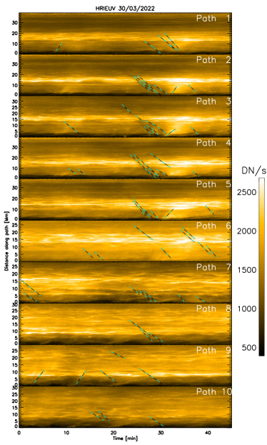
Figure 9: Time-distance diagrams for all coronal rain paths shown in the left panel of Figure 1. The cyan-black dashed lines with negative slopes show some of the tracks produced by the rain clumps as they fall. The lines are offset in time by 1 minute to better see the rain features. Note the extent of the rain shower across all paths. Upward propagating features (positive slopes) can also be seen, particularly at the end of the rain shower ($t\approx 30\leavevmode\nobreak\$min). Zero distance corresponds to the footpoint of the loop (seen in Figure 4).

4.4 Rebound shock and flow

Figure 6 (lower panel) shows another interesting feature of the event from March 30, also seen in the animation of Figure 4. Following the impact on the chromosphere of the rain shower a bright upward propagating feature can be seen. We interpret this as a rebound shock and flow produced by the rain impact. To the best of our knowledge, this is the first time that such feature is observed, despite being predicted by every numerical simulation of coronal rain (e.g. Müller et al., 2003; Fang et al., 2015). This feature can also be seen in each time-distance diagram of Figure 8 as a bright upward slope just after the end of the rain shower. The slope indicates speeds between $50-130$ km s^-1. The lower end of this velocity range matches the expected value for upward flows, while the upper end matches the tube speed for a plasma temperature of $10^{5.8}$ K, which is close to the temperature at the peak of the Fe X 174 Å  formation. This is also supported by numerical simulations (Antolin et al., 2022).

4.5 Extent of the rain shower

To examine the extent of the rain shower we plot in Figure 9 the time-distance diagrams corresponding to all the paths shown in Figure 4. Several clump tracks are shown by dashed lines. We can see that the main rain shower occurs in the time range $t=20-30$ min. Although it can best be seen in paths 2 to 5 we can still traces of it across all the paths. This indicates that the extent of the rain shower across the loop bundle is at least 15 Mm in the POS, and possibly larger given the observed expansion of the loop bundle seen in Figure 1 (left panel). This is supported by the SPICE observations in Figure 5, which show cool transition region emission over a width larger than that set by the rain clumps detected by HRI_EUV. Along the loop, the clumps can be tracked for up to 25 Mm. Note that many clumps are only clearly visible in the last 10 Mm, suggesting that the catastrophic cooling is non-uniform, with accelerated cooling rates down to chromospheric temperatures being more confined in the transverse direction. This effect may also be due to the line-of-sight, as shown in section 4.13.

Figure 9 also shows that the rebound shock and flow occurs across a wide expanse, but appears more concentrated than the rain shower and can only be clearly seen in paths $1-6$.

4.6 Region 1 of April 1 - a large coronal rain event

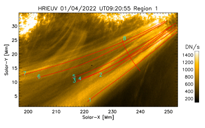
Figure 10: Close-up on the footpoint of a large coronal loop bundle observed on 2022 April 1 by HRI_EUV. The FOV corresponds to that of Region 1 indicated by the white rectangle in Figure 1, right panel. Except for path 8 (which crosses the loop bundle), the red paths denote several rain paths. An animation of this figure is available, whose images have been processed with the wavelet-optimized whitening enhancement technique of Auchère et al. (2023). It runs from UT09:19 to UT10:34 and shows several rain clumps falling towards the chromosphere. The movie first runs without and then with the rain paths overlaid.

We now turn our attention to some of the coronal rain events seen on the April 1 dataset (see Figure 1, right panel).

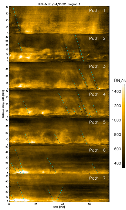
Figure 36: Time-distance diagram for the rain paths tracked in Region 1 shown in Figure 10. The cyan-black dashed lines with negative slopes track the dark/bright absorption/emission features produced by several rain clumps falling into the chromosphere. A few bright upward propagating features can also be seen (positive slopes). Zero distance corresponds to the footpoint of the loop (top-right of Figure 10).

In Figure 10 we show the close-up on the footpoint of the large coronal loop bundle undergoing a global change (akin to shrinkage), denoted as Region 1 in Figure 1 (right). We follow several rain clumps and plot in Figure 36 the corresponding time-distance diagrams. A main shower event is seen in the time range $t=40-70$ min particularly along paths $2-4$, but signatures of another rain shower are also seen at the beginning ($t<20$ min), particularly along paths $6-7$. Also in this case, a combination of neighboring dark and bright paths can be seen. Although not as clear as for the March 30 event, some of the bright tracks may correspond to the downstream compression and heating, especially those that immediately precede the absorption feature. Note that some of these tracks only appear bright, for example the last track of Path 6. Furthermore, upward propagating features can also be observed, some of which do seem to appear just after rain impact. The observed morphology and speeds are similar to those seen for the March 30 event, all of which are calculated and presented in Section 4.11.

The rain shower seen in Region 1 appears to be far wider in extent than that of March 30. As seen in Figure 10, the transverse length across which the clumps are seen is at least 20 Mm, but certainly greater given the observed expansion. Furthermore, the clumps can be followed for longer lengths along the loop, with some being tracked for over 40 Mm. This suggests catastrophic cooling down to chromospheric temperatures over a larger coronal volume, which is supported by SPICE observations.

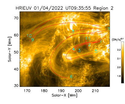
Figure 11: FOV corresponding to Region 2, shown in Figure 1 (right panel). The red curves correspond to paths of some of the observed coronal rain clumps. Note that intensities are scaled with a power of 0.1 to see a larger range of variations. An animation of this figure is available, whose images have been processed with the wavelet-optimized whitening enhancement technique of Auchère et al. (2023). It runs from UT09:19 to UT10:34 and shows several rain clumps falling towards the chromosphere. The movie first runs without and then with the rain paths overlaid.

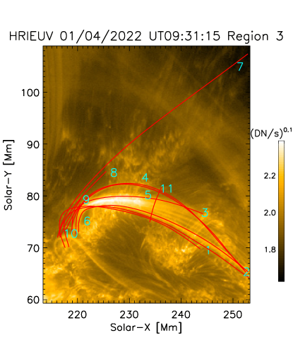
Figure 12: FOV of Region 3 shown in Figure 1 (right panel). The red curves correspond to paths of some of the observed coronal rain clumps. Paths 1 to 6 belong to the bright loop in the lower half of the image, while paths 7 to 10 belong to a very long loop going towards the top right corner of the image. Paths 9 and 10 are very short and parallel to each other. Note that intensities are scaled with a power of 0.1 to see a larger range of variations. An animation of this figure is available, whose images have been processed with the wavelet-optimized whitening enhancement technique of Auchère et al. (2023). It runs from UT09:19 to UT10:34 and shows several brightenings followed by mostly bright rain clumps falling towards the chromosphere. The movie first runs without and then with the rain paths overlaid.

4.7 Region 2 of April 1 - null-point topology at footpoint

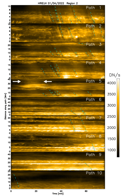
Figure 37: Time-distance diagrams for the paths of the rain clumps shown in Figure 11. The cyan-black dashed lines correspond to coronal rain tracks along the paths, with zero distance corresponding to the loop footpoints on the right side in Figure 11. The lines are offset in time by 1 min to better see the rain features.The white arrows in the time-distance diagrams for path 5 indicate the times when the loop brightens prior to the appearance of the rain.

Region 2 on April 1 shows several coronal rain events belonging to different regions in the AR. In Figure 11 we show the FOV corresponding to Region 2, as shown in the full FOV of Figure 1 (right panel), with several rain clump paths overlaid. The corresponding time-distance diagrams for these paths are shown in Figure 37.

The most interesting rain shower is tracked by paths $1-5$ in these figures. First, a loop bundle appears, with the intensity all along the loop increasing in a uniform manner (but particularly at the apex) around UT 09:30 (about 10 min from the start of the observation). This brightening can be best seen along path 5 (white arrows in Figure 37). The intensity uniformly decreases along the loop over the next 10 min, after which, the first rain clumps appear, with the bulk of the rain seen after 20 min from the first intensity increase. Following the rain shower impact, the intensity increases strongly at the footpoint with some signatures of upward propagating features (red arrow in Figure 37)). As the rain falls, it is observed to strongly deviate from its path and spread in different directions, reminiscent of a null-point topology structure at the footpoint.

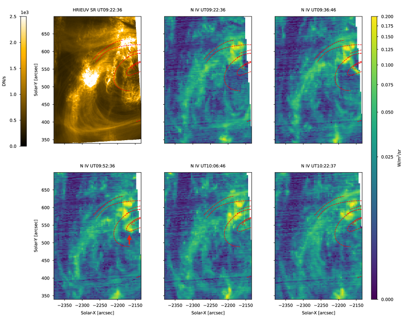
Figure 13: SPICE rasters in the N IV line ($\log T=5.2$ K) over a region that overlaps with Regions 1 and 2 on April 1. The FOV corresponds to the red rectangle to the East shown in Figure 2 (bottom) and the overlaid red curves denote some of the rain paths seen with HRI_EUV (see Figures 10 and 11). The HRI_EUV panel corresponds to a synthetic raster matching the time of the first SPICE raster (see text for details) but preserving the HRI_EUV spatial resolution. The SPICE panels show the total intensity integrated over the N IV spectral line for each raster (time shown in subtitle). The brightening indicated by the red arrow in the UT09:52:36 panel corresponds to cooling through the passband.

The paths $6-7$ and possibly path 8 seem to correspond to another loop bundle that also experiences a similar uniform and global loop brightening as described above. In this case, the loop bundle brightens at the very start of the observation, and disappears after almost 1 hr. The rain is seen roughly 50 min after the start of the brightening, but is much fainter in terms of EUV absorption than for the previous case. This loop is rooted close to a pore, and periodic upward/downward ballistic motion is seen (particularly for paths 7 and 8), characteristic of Type 1 spicules (Beckers, 1964) or the EUV counterparts of AR dynamic fibrils (Mandal et al., 2022).

Path $9$ (and possibly path 8 as well) may correspond to the other footpoint of the large loop bundle of Region 1. However, contrary to the other footpoint, the amount of rain that can be observed falling into this footpoint is minimal and is further very faint.

The last path 10 may also belong to the large loop bundle of Region 1, and the location of its footpoint is uncertain. Instead of the region where the previous paths are rooted, path 10 appears to be rooted in a moss. Minimal rain events are seen in this case.

All rain tracks observed in Region 2 show mostly EUV absorption, with little EUV emission of the kind described earlier associated with compression. Also, most tracks are relatively short ($10-20\leavevmode\nobreak\$Mm) when compared to Region 1, which may be due to the different inclination of the loops relative to the LOS.

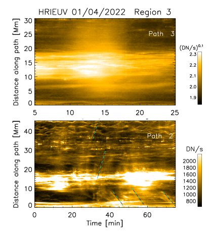
Figure 14: Top: Loop brightening prior to a coronal rain event. This time-distance diagram (close up on the time range $t=[5,25]\leavevmode\nobreak\$min) corresponds to path 3 in Region 3 on April 1 shown in Figure 38. Note that the intensities have been scaled to the power of 0.1 to better see the large intensity variation. Bottom: Time-distance along path 2 in the same lop bundle. The white dashed lines correspond to dark and bright tracks from coronal rain.

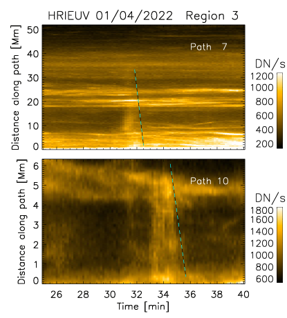
Figure 15: Close-up on the time range $t=[25,45]\leavevmode\nobreak\$min in the time-distance diagram of paths 7 (top) and 10 (bottom) shown in Figure 38. Note that the beginning of the brightening at $t\approx 33$ min starts essentially at the same time along the path. The cyan-black dashed lines trace the outer envelope of the brightening indicating a speed of $\approx 150\leavevmode\nobreak\$km s^-1.

4.8 SPICE view on Regions 1 and 2

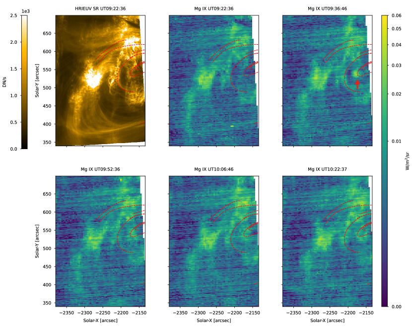
Figure 26: Same as in Figure 13 but for the Mg IX line.

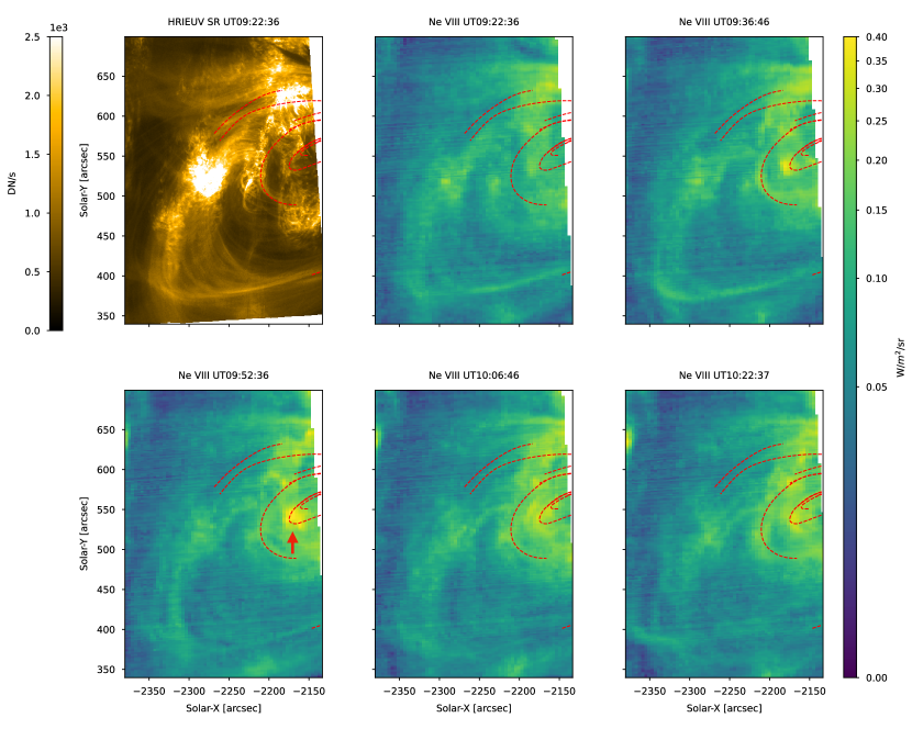
Figure 27: Same as in Figure 13 but for the Ne VIII line.

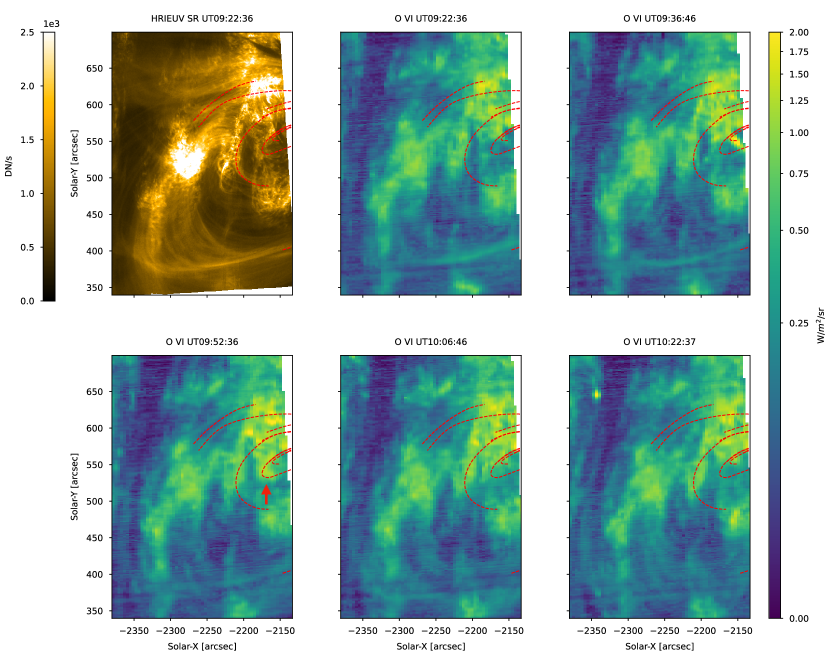
Figure 28: Same as in Figure 13 but for the O VI line.

The SPICE rasters managed to capture part of the regions of interest observed with HRI_EUV on April 1. This includes the top part of Region 1 and most of Region 2 (see Figure 2, bottom), which mostly correspond to the apexes of the loops with coronal rain. These loops are barely visible in the Mg IX coronal line (Figure 26) but their filamentary structure are well seen in the upper transition region lines (Ne VIII, O VI in Figures 27 and 28). Furthermore, emission similar in morphology and strong variability can also be seen in the lower transition region N IV line (Figure 13). For instance, the large-scale brightening in the loop that corresponds to paths 1 to 5 in Region 2 (described in section 4.7) can be seen to peak in Mg IX at UT09:36 (red arrow in the corresponding Figure), while in Ne VIII, O VI and N IV the brightening peaks at UT09:52, and in C III the peak is sseen at UT10:06 (with some hints of increased brightness in Lyman-$\beta$ as well but inconclusive due to the strong background). This strongly supports our interpretation of cooling through the passbands of HRI_EUV and SPICE and subsequent appearance of rain in EUV absorption.

4.9 Region 3 of April 1 - Localised and large-scale flash-like EUV emission from rain

Figure 12 shows Region 3, as denoted in the full FOV of Figure 1 (right panel), with several rain paths overlaid. Most of the loops analysed in Region 3 show a very different inclination with respect to the LOS when compared to the previous cases. In this case, the LOS appears much less inclined with the loop plane, leading to a top view of the loop rather than a sideways view. Consequently, while the footpoint legs appear very short, the apexes appear long in the projected view.

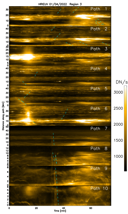
Figure 38: Time-distance diagrams for the paths of the rain clumps shown in Figure 12. The cyan dashed lines correspond to coronal rain tracks along the paths, with zero distance corresponding to the loop footpoints (left in Figure 12). The lines are offset in time by 1 min to better see the rain features. Note the loop brightening seen clearly in Paths 3 and 6 at time $t=15\leavevmode\nobreak\ min$.

Paths $1-6$ appear to correspond to the same loop bundle, although paths $4-5$ show slightly different trajectories relative to paths $1-3$, which may be indicative of braiding. This is further supported by the AIA observations of the same event, as discussed in Section 4.13. As for the loops in Region 2, a strong EUV enhancement uniformly along several coronal strands composing the loop bundle are seen roughly 10 min from the start of the observation. The coronal strands appear extremely thin, with sub-arcsecond widths (see section 4.12). This brightening can be clearly seen in the time-distance diagrams shown in Figure 38. Most of the coronal strands disappear 20 min later. Both dark and bright tracks can be seen in most time-distance diagrams, indicative of flows in both directions (towards both footpoints). Some appear at the start of the global intensity enhancement and others appear $20-60$ min after. Note that despite the very close proximity of paths 1 and 2 and paths 4 and 5, they show different (dim) features in their evolution. AIA 304 confirms the presence of rain along this loop bundle (Section 4.13).

Path 3 corresponds to one of the best visible coronal strands. As shown in the time-distance diagram, no clear bright or dark track can be seen. We select this path to more accurately investigate the uniform global intensity enhancement common to many of the strands in the loop bundle. In Figure 14 (top) we show the part of the time-distance diagram corresponding to the intensity enhancement for path 3. Compared to the background, the enhancement appears diffuse and seems to start close to the apex and propagates towards both footpoints in a couple of minutes. Overall, this global intensity enhancement over the strand lasts $\approx 8\leavevmode\nobreak\$min. In Figure 14 (bottom) we show a similar case for path 2. However, in this case about 4 intensity enhancements are observed and almost all are accompanied by dark or bright propagating features.

Although many of the features in paths $1-6$ do not show the EUV absorption, but rather emission, we still associate them with coronal rain. Besides similar velocities (see Section 4.11), the AIA observations of the same event provide conclusive proof (Section 4.13).

The last set of paths we analyse are paths $7-10$, which correspond to a different loop, apparently much larger in size. We were able to track a bright clumpy feature over 40 Mm, leading to path 7. The clump falls at speeds of $\approx$150 km s^-1 in the POS, which, to our knowledge, is the fastest ever recorded speed for a falling clump with imaging devices (besides erupting fall-back). Just prior to impact, over the last $5-15$ Mm, several other clumps are seen along parallel paths (tracks in paths 8, 9 and 10), suggesting that the catastrophic cooling into chromospheric temperatures takes longer for these neighboring strands.

In Figure 15 we show a close-up of the time-distance diagram corresponding to paths 7 (top) and 10 (bottom) over the time where the falling clump is observed. The bottom panel in the figure shows a very interesting pattern. While the outer envelope (traced by the cyan-black dashed line in the figure) corresponds to the same speed as observed in the longer time-distance path of path 7 (top panel), there is an almost instantaneous intensity increase all along the path at time $t\approx 33$ min. We believe that this feature is due to the compression of the rain downstream, that is, physically similar to the small brightening observed for the March 30 rain clumps. However, while the brightening for the latter is always immediately below the rain’s head, for the present case it occupies a much larger longitudinal extent. This is probably due to a much stronger compression, which is able to increase the temperature of the entire region below the rain to a temperature close to the emissivity peak of HRI_EUV ($\log T=5.8-6$), thereby generating a flash-effect.

4.10 Region 4 - Off-limb coronal rain

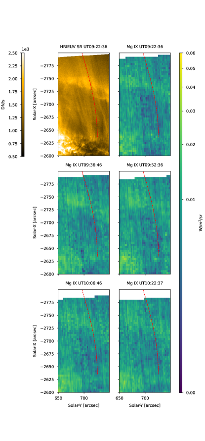
Figure 31: Same as in Figure 17 but for the Mg IX line.

On April 1 HRI_EUV captures various long loops rooted in the trailing AR closer to the limb. Small EUV absorption features falling towards the surface can be seen in one such loop, which we follow and show in red within Region 4 shown in Figure 1. The time-distance diagram along this path is shown in Figure 16, where various characteristic dark and bright tracks of coronal rain can be seen falling at projected speeds of $50-90$ km s^-1. This loop is also partly visible in the SPICE rasters of April 1. In Figures 31 to 35 we show the evolution through the SPICE rasters of the emission in this region. In particular we notice strong variability in the upper and lower transition region (Ne VIII, O VI, N IV) and chromospheric emission (C III and Lyman-$\beta$) as shown in Figure 17. Therefore, SPICE confirms the presence of coronal rain emitting at transition region and chromospheric temperatures in this loop.

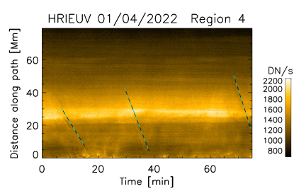
Figure 16: Time-distance diagram along a loop observed partly off-limb by HRI_EUV on April 1. The path corresponds to red curve in Region 4 shown in Figure 1. The cyan and black dashed lines correspond to dark and bright tracks from coronal rain (offset in time by 1 min in the figure for better visualisation).

Figure 17: SPICE rasters in the C III line ($\log T=4.8$ K) over a region that overlaps with Region 4 on April 1. The FOV corresponds to the red rectangle to the East shown in Figure 2 (bottom) and the overlaid red curves denote some of the rain paths seen with HRI_EUV (see Figures 10 and 11). The HRI_EUV panel corresponds to a synthetic raster (SR) matching the time of the first SPICE raster (see text for details) but preserving the HRI_EUV spatial resolution. The SPICE panels show the total intensity integrated over the C III spectral line for each raster (time shown in subtitle).

4.11 Statistics

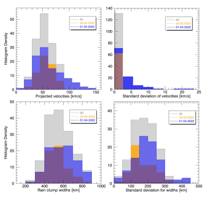
Figure 18: Projected velocities (top) and widths (bottom) and associated standard deviation (corresponding right panels) for all rain clumps tracked in this work. The colours include transparency and denote different dates (see legends).

In this section we provide statistics of all the velocity and width measurements on the coronal rain clumps (both in absorption and in emission). Please see Section 3 for the methods on how these quantities were calculated.

In Figure 18 we show a histogram of all the measured projected velocities for both datasets. We note that the peak of the distribution is between $40-60$ km s^-1, with speeds as low as 10 km s^-1 and as high as 150 km s^-1. The latter high projected velocities are not common for coronal rain, and may well constitute the highest projected velocities to date (note that eruptive prominence fallback is not coronal rain). No major differences exist between both dates, except that April 1 presents a bigger spread, which is normal given the higher number of rain events analysed for that date. The bulk of the distribution matches well with previously reported speeds (Antolin & Rouppe van der Voort, 2012; Schad, 2017; Antolin & Froment, 2022), as well as those obtained in numerical simulations (Fang et al., 2015; Li et al., 2022). As shown in the figure, the errors in the velocity measurements are generally small (on the order of 5 km s^-1 for most).

Similarly, in Figure 18 we show a histogram of all measured rain clump widths. The distribution peaks between $400-600$ km, but goes as low as 260 km and as high as 890 km. Both dates present small differences in terms of distribution shape. While both datasets have relatively small pools, the dataset of Aptil 1 presents a broader distribution with values about 100 km larger. The standard deviation figure indicates that there is a relatively large variation or error in the width measurement. This is not unexpected, since along a given track the rain clump’s background varies significantly, leading to differences in the results of the Gaussian fits (despite efforts in reducing the background influence, see Section 3).

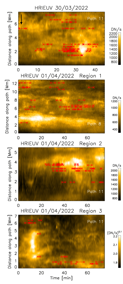
Figure 19: Time-distance diagram along paths that cross several loop bundles: path 11 in Figure 4 (top), path 8 in Figure 10 (second panel from top), path 11 in Figure 11 (third panel from top) and path 11 in Figure 12 (bottom). The red lines between crosses denote times and location at which rain clumps are observed. The vertical black arrow in the top panel indicates an example of an EUV absorption feature produced by a rain clump. Note that the intensities in the bottom panel have been scaled to the power of 0.1 to better see the large intensity variation.

4.12 Coronal strands associated with coronal rain

To investigate more carefully a possible relation between the filamentary coronal structure (coronal strands) within loop bundles and the coronal rain they host, we take cuts across several of the analysed loop bundles, as shown in Figures 4 (path 11), 10 (path 8), 11 (path 11) and 12 (path 11). We show the resulting time-distance diagrams along these cross-cuts in Figure 19.

Several coronal strands can be seen in each Figure, some of which very likely belong to the loop bundle hosting the rain event. In many instances, as the rain crosses the transverse cuts it produces a small absorption feature (whose time duration depends on the clump’s length as speed). One example of such a feature is shown by an arow in Figure 19. Note that it is preceded and followed by a bright EUV feature of roughly the same width as the rain clump. A large group of rain clumps is seen around $t=22-32$ min, followed by a bright feature at $t=32-40$ min. This bright feature corresponds to the rebound shock and upward flow produced by the rain shower impact.

In Figure 19 a group of strands can be seen appearing after $t=30\leavevmode\nobreak\$min between distance 5 and 8 Mm across the transverse cut, which seems to coincide with the location in time and space of a group of rain clumps. Similarly, in the other panels in the Figure the rain clumps appear to be preferentially located in regions where coronal strands are observed. While sometimes a 1-to-1 association between a coronal strand and a rain clump can be made (particularly for the latter), it is not the general case. However, we can notice that the widths of coronal strands (around 500 km) are on average similar to rain clump widths.

4.13 SDO/AIA observations at different line-of-sight and resolution

Our investigation on the coronal rain events with HRI_EUV is complemented by co-temporal SDO/AIA observations. On these dates, Solar Orbiter was in quadrature with SDO, thereby offering a different view on the same ARs. In Figures 20 and 22 we show snapshots for March 30 and April 1, respectively, with a FOV centred on the regions of interest. The same large-scale coronal structures can be identified across both instruments.

Despite the similarity between AIA 171 and HRI_EUV in terms of the emission, and the large-scale nature of the event (occurring across at least 15 Mm in HRI_EUV), no clear downflow can be observed in absorption or emission with AIA 171 on March 30 over the same time period. Sections of the loop bundle appear and disappear over the same duration, which likely correspond to the EUV variation associated with coronal rain observed with HRI_EUV. Some upward flows, bright in EUV, are observed, which could correspond to the rebound shock and flow observed with HRI_EUV. To check this we have identified and tracked a few large rain clumps in AIA 304, whose paths are shown in Figure 20. The time-distance diagrams along these paths are shown in Figure 21 and we can easily identify the characteristic rain slopes in AIA 304 (tracks in the time-distance diagrams). Note the brightenings at the times the rain impacts the chromosphere. With the help of AIA 304 we are able to recognise the rain features in AIA 171, such as EUV absorption and in particular a rebound shock and flow feature following the rain impact. The strong EUV variation that is seen in the image sequence is therefore attributable to the rain episode.

On April 1, only region 1 shows clear coronal rain in the image sequence of AIA 171, with the characteristic EUV absorption features downflowing along the loop. Regions 2 and 3 show very similar EUV variation as observed with HRI_EUV, but as for March 30, we were unable to directly identify coronal rain downflows only based on EUV absorption features in the image sequences. However, the expected coronal rain is revealed in the 304 channel and we were able to roughly identify the large-scale coronal rain events for each of the loops. As for March 30, we track several large rain clumps in each region (shown in Figure 22) and plot the time-distance diagrams in Figure 23. Path 1 tracks a rain clump belonging to Region 1’s loop, paths 2 and 3 belong to Region 2 and may correspond to the loops outlined by paths 8 and 9 in Figure 11, and paths 4 and 5 follow clumps in the loop bundle outlined by paths 1 to 6 in Figure 12. We are able to detect several rain tracks in the time-distance diagrams of AIA 304 and a very clear EUV absorption profile in AIA 171 for path 1. However, the signatures in AIA 171 are much harder to detect. In paths 2 and 4 we do not see any features of the rain falling in AIA 171, but a bright feature can be seen near the footpoint of path 4 that may correspond to the impact and rebound shock and flow from a rain shower. In paths 3 and 5 we are able to recognise a few EUV absorption and emission tracks co-temporal and co-spatial to the rain tracks in AIA 304. The bright EUV emission in 171 is similar to that seen in HRI_EUV in paths 1 or 6 of Figure 38, in that a large-scale emission is seen simultaneously all along the path that precedes the bright downflowing feature from the rain.

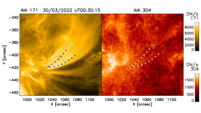
Figure 20: SDO/AIA observation in the 171 (left) and 304 (right) channels of the March 30 coronal rain event. AIA was roughly in quadrature with Solar Orbiter on this date. The large loop bundle observed in the AIA 171 map corresponds to the same loop bundle observed by HRI_EUV in Figure 4. The white-black dashed paths follow some rain clumps observed in AIA 304. An animation corresponding to this figure is available. The animation shows several rain clumps in AIA 304 but no clear counterpart is seen in AIA 171, although strong intensity variations are observed at the same locations. The animation runs from UT00:02 to UT00:49 and comprises the time where coronal rain is observed with HRI_EUV. It first runs without and then with the rain paths overlaid.

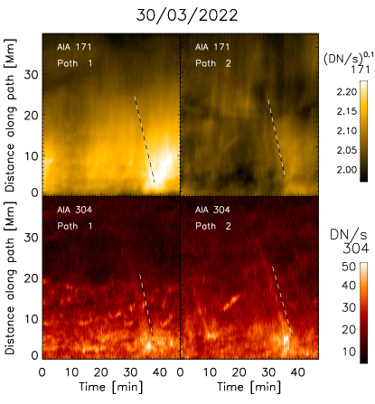
Figure 21: Time distance diagrams along paths 1 and 2 shown in Figure 20 on March 30, with AIA 171 (top) and AIA 304 (bottom). Dark and bright paths from coronal rain are highlighted with white-black dashed lines, which are offset by a fraction of a minute to better see the rain features. Zero distance corresponds to the footpoints of the loops. Note that the AIA 171 intensities have been scaled to the power of 0.1 to better see the large intensity variation.

It is interesting to note that, as shown by the AIA 304 animation, there is widespread coronal rain over the AR over the same FOV as HRI_EUV and including loops for which it is not observed with HRI_EUV. A large amount of coronal emission ahead of the rain along the LOS can easily decrease the contrast produced by EUV absorption or emission from the rain in the 171 or 174 channels, thereby making it undetectable. As we show here, high spatial resolution can help retaining this contrast, which is why we observe far more in HRI_EUV than AIA 171. On the other hand, AIA 304 shows the emission/absorption from the rain more directly since no further emission is present ahead of the rain along the LOS. Nevertheless the rain can be hard to discern due to the very bright TR background in AIA 304.

The larger FOV provided by SDO/AIA sheds more light into the large-scale magnetic structure of Region 1 on April 1. AIA 171 reveals a topology akin to null-point topology, with open field lines (or much larger loops) above, with the loop arcade below the null-point. This provides an explanation to both the large-scale reconfiguration and the observed large-scale coronal rain event in the loop, with continuous coronal rain over a very wide loop cross-section observed for the entirety of the HRI_EUV observation. Indeed, as discussed in Li et al. (2018); Mason et al. (2019), magnetic dips are often observed above null-point topologies, which act as mass reservoirs where large amounts of material can catastrophically cool down. The cool and dense material can then either spill sideways from the magnetic dip or flow through the null-point, facilitated by the reconnection process, downward into the newly formed reconnected loops. This process can be very long-lived (Chitta, L. P. et al., 2016; Chen et al., 2022) and can be accompanied by a reconfiguration of the loop, similar to shrinkage (as in the standard flare model).

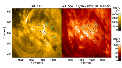
Figure 22: SDO/AIA observation in the 171 (left) and 304 (right) channels of the April 1 coronal rain events. AIA was roughly in quadrature with Solar Orbiter on this date. Some of the large loop bundles observed by HRI_EUV can be easily identified. The white-black dashed paths follow some rain clumps belonging to these loop bundles, observed in AIA 304. Path 1 follows the same loop bundle seen in Region 1 of Figure 10. Paths 2 and 3 may correspond to the same rain events shown in paths 8 or 9 in Region 2 of Figure 11. Paths 4 and 5 follow the same loop bundle shown in the lower part of Figure 12 (paths 1 to 6 in that Figure). An animation corresponding to this figure is available. The animation shows widespread rain in AIA 304 but the counterparts in AIA 171 can only clearly be seen for the loop around path 1, although strong intensity variations are observed at the same locations. The animation runs from UT09:20 to UT10:32 and comprises the time where coronal rain is observed with HRI_EUV. It first runs without and then with the rain paths overlaid.

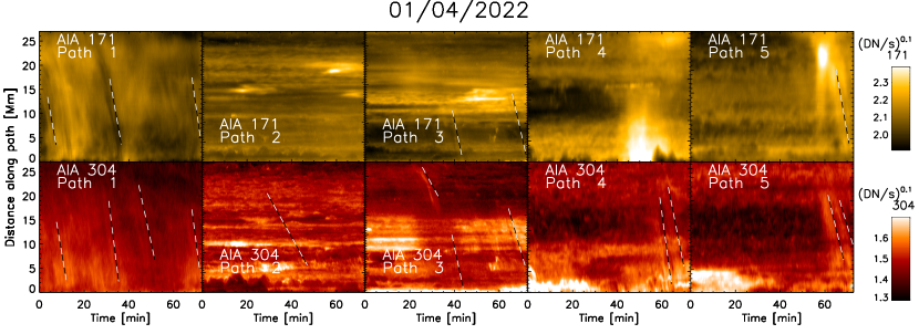
Figure 23: Time distance diagrams along paths 1 to 5 shown in Figure 22 on April 1, with AIA 171 (top) and AIA 304 (bottom). Dark and bright paths from coronal rain are highlighted with white-black dashed lines, which are offset in time by 1 min to better see the rain features. Zero distance corresponds to the footpoints of the loops. Note that the intensities have been scaled to the power of 0.1 to better see the large intensity variation.

4.14 Widespread coronal rain as suggested by SPICE

All the loops with coronal rain captured with HRI_EUV show clear counterparts in SPICE in the upper and lower transition region lines. For the off-limb loop of Region 4 we were also able to capture clear emission in the chromospheric lines of SPICE, thanks to the lower background emission. In Figure 24 we show a multi-wavelength view of the full FOV of SPICE for 1 raster. What is striking of this figure is that cool loops emitting in the upper and lower transition region lines, with similar features (morphology, variability) as those where we have detected coronal rain, are widespread in the FOV. Indeed, all the 5 rasters of this region show strong variability in these loops. This strongly suggests that at least for this AR coronal rain is widespread and that only a fraction of it is observed in EUV absorption with HRI_EUV. This matches also the picture obtained with AIA 304.

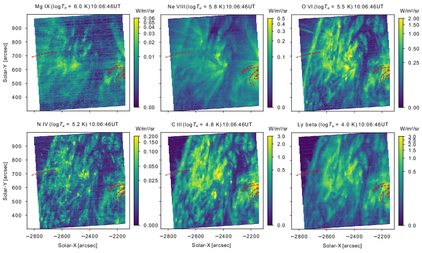
Figure 24: SPICE multi-wavelength full FOV on April 1. The SPICE FOV is the same as that shown in Figure 2 (bottom), co-aligned with HRI_EUV. The overlaid red curves denote some of the rain paths seen with HRI_EUV (see Figures 10 and 11). Each SPICE panel shows the total intensity over a spectral line indicated in the subtitle, together with its temperature of maximum formation.

5 Discussion and Conclusions

In this work we analysed coronal rain at unprecedented spatial resolution in the EUV, provided by Solar Orbiter observations with HRI_EUV during the 2022 spring perihelion. Observations were complemented with SPICE and AIA, providing a multi-wavelength picture of the phenomenon in various active regions. The resolution achieved is $\approx 240\leavevmode\nobreak\$km, which is only about two times lower than previous H$\alpha$ observations of the phenomenon with the SST (Antolin & Rouppe van der Voort, 2012). The strong correlation between EUV absorption and H$\alpha$ emission, expected from radiative transfer theory (Anzer & Heinzel, 2005), is here confirmed down to the smallest resolved scales ever achieved, with clump FWHM widths as small as 260 km. This fine-scale structure is also reflected in the fact that many clumps only produce very faint EUV absorption features, thereby requiring high-resolution and sensitivity to detect them.

We selected 2 dates on which Solar Orbiter observed several ARs on-disk and partly off-limb. On March 30 we focused our attention on one coronal loop bundle and discovered new features of coronal rain dynamics. As the rain falls, the region immediately beneath the clump (downstream) is observed to brighten, leading to very fine light streaks in time-distance diagrams. We interpret this phenomenon as being the result of compression and heating due to the relatively large momentum of the condensation. Fang et al. (2015) report the formation of rebound shocks when coronal rain forms, produced by the localised loss of pressure driving strong flows that lead to the condensation. These rebound shocks may be thought as the source of the brightening that we see. However, the rebound shocks are then seen to propagate away at the sound speed from both sides of a condensation, much faster than the condensation’s falling speeds. There is no reason why these rebound shocks should propagate at the same speed. Therefore these rebound shocks cannot explain our observations. On the other hand, our interpretation as commpression and heating is supported by 2.5-D MHD simulations of coronal rain by Li et al. (2022, see their Figure 4) and Antolin et al. (2022). This phenomenon is therefore similar to the fireball phenomenon on Earth linked to meteoric ablation, with the region below the clump being compressed and heated as it falls. We do not observe this phenomenon for all coronal rain events, which suggests that not only a high spatial resolution is needed but also favorable line-of-sight relative to the rain trajectory. It is also possible that the compressed material exists in all cases but emits at different temperatures not sampled by HRI_EUV.

EUV enhancement associated with coronal rain is also observed during the fall ahead and at the wake of rain clumps. The latter can be seen in the time-distance diagrams along or across rain clump trajectories as an increase of the EUV intensity that follows the EUV absorption feature. This may correspond to a coronal strand and is likely due to the CCTR, which extends from the clump far into the wake, as shown by numerical simulations (Antolin et al., 2022; Li et al., 2022). Observations with SPICE show the filamentary structure in the upper and lower transition region lines, thereby supporting this interpretation. Ahead of the clump, besides the fireball feature, a second, more elusive kind of brightening is observed just prior to the rain impact (with the brightening spreading over $\approx 6$ Mm), and manifests as a flash-like simultaneous intensity enhancement of the entire space between the clump and the chromosphere. We suspect that this is also due to the compression of the plasma ahead of the clump, as suggested by the same numerical simulations cited previously, with a compression strong enough as to increase the temperature of the entire region below the rain close to the emissivity peak of HRI_EUV ($\log T=5.8-6$), thereby generating a flash-effect. However, we only found one clear occurrence of this larger-scale compression, for which the rain is extremely fast (with projected speeds of 150 km s^-1). Such speeds may be supersonic, in which case the compression argument may not fully explain it. Indeed, if produced by compression, it means that sound waves are produced ahead of the clump and travel fast enough to compress the entire region donwstream (leading to the ‘flash-like’ character of the brightening). However, this is not possible if the clumps are supersonic.

Another new phenomenon is the rebound shock and upflow that follows the rain impact onto the chromosphere. The feature is detected best after the end of rain showers rather than individual rain clumps, and is characterised by a bright and diffuse propagating EUV feature roughly along the same paths over which the cool downflows occur. The propagating speeds are between $50-130$ km s^-1, depending on the selected path for the time-distance diagram. Based on multi-dimensional simulations of this phenomenon (Antolin et al., 2022), we suspect that this difference is due to the combination of the rebound shock, which propagates at the tube speed of $\approx 130\leavevmode\nobreak\$km s^-1 (for temperatures corresponding to the Fe X 174 Å  formation temperature of $10^{5.98}$ K), and an upward flow produced by the impact (which are bound by gravity and thus slower). To the best of our knowledge, this is the first report of this effect, despite being predicted by numerical simulations for decades (Müller et al., 2003; Mendoza-Briceño et al., 2002; Antolin et al., 2010; Fang et al., 2015; Li et al., 2022). Indeed, we expect a response from the lower atmosphere in the form of an upflow or upward propagating wave along every magnetic field line and probably even over a wider region compared to that affected by the rain impact, due to the high-$\beta$ conditions and strong gas pressure increase at the chromospheric heights of rain impact (Antolin et al., 2022). For the March 30 event, this upward propagating feature is seen to reheat the loop bundle and may correspond to the start of a new TNE cycle. Simulations indicate that efficient refilling and reheating of the loop is only obtained in the case that the stratified heating is still on-going. In other words, if there is no continuous heating at the loop footpoint, the simple rebound shock and flow obtained from a rain shower is insufficient to bring the density and temperature back to usual coronal values. The rebound shock and upflow can be seen mainly after rain showers rather than individual rain clumps, suggesting an additional feedback effect from the large rain shower momentum. Only a subset of rain showers show these features, despite their relatively large-scale nature, indicating that the conditions to observe this atmospheric response to the rain impact are stringent. This is further supported by the AIA 171 co-temporal observations on March 30 in quadrature with HRI_EUV, where some hints of an upward propagating disturbance are observed but remain much dimmer and elusive.

As shown by Şahin & Antolin (2022), rain showers can help identify coronal loop entities (defined as a coronal volume evolving in similar way and therefore subject to similar heating conditions). This is particularly important given the optically thin nature of the corona, leading to great LOS superposition (also referred to as ‘the coronal veil’; Malanushenko et al., 2022). Furthermore, the occurrence of coronal rain points to a state of TNE, for which stringent coronal heating conditions are needed. This is particularly the case of quiescent coronal rain, which occurs in usual coronal loops and is accompanied by long-period intensity pulsations for long-duration heating (Froment et al., 2020). It is still unclear whether the TNE-TI scenario still applies to prominence-coronal rain hybrid structures (although initial results indicate quasi-periodic occurrence that may correspond to long-period intensity pulsations Li et al., 2019) or even to flare-driven rain.

Klimchuk & Luna (2019) have quantified the conditions for TNE, which include a strong heating stratification (ratio of apex-to-footpoint volumetric heating rate below 0.1) and not too high heating asymmetry between footpoints (below 3, to prevent siphon flows that effectively reduce the lifetime of the condensations in the corona relative to their falling time). Johnston et al. (2019) further show that a high frequency rate for the heating events (with repeating time less than the radiative cooling time of the loop) is needed. Several of the observed rain showers in this work occur following a global brightening of the loop. This is expected from the TNE-TI cycle, in which the loops start at a hot, indeterminate temperature and radiatively cool down. What is observed then corresponds to the loop’s temperature going through the temperature response range of the HRI_EUV channel, which peaks at $\approx 10^{6}$ K (Rochus et al., 2020). Usual draining and cooling of loops would explain this global brightening feature, but would fail to explain the appearance of the clumpy downflows in EUV absorption or emission that follow the global brightening events (Peter et al., 2012). This is also the case in post-flare cooling, where simple draining and global cooling of loops is unable to explain flare-driven rain (Reep et al., 2020). Our cooling interpretation is further supported by the SPICE observations, which show that the brightening is delayed for cooler spectral lines at transition region and chromospheric temperatures.

It is interesting to note that the observed global brightening occurs fairly uniformly and symmetrically along the loop, with the apex brightening a few minutes prior to the rest of the loop. To our knowledge, very few works investigate in detail (including the necessary forward modelling into e.g. AIA 171) the spatial distribution of the cooling during TNE cycles. The published literature indicate that we should expect symmetric global brightening in a channel such as AIA 171 during the cooling stage of TNE cycles when the heating is symmetric across both footpoints (Müller et al., 2003; Peter et al., 2012; Winebarger et al., 2018; Johnston et al., 2019), while asymmetric heating or loop geometry may tend to produce asymmetric global brightening, with significant brightening only along one loop leg (Mikić et al., 2013; Froment et al., 2018; Pelouze et al., 2022). This would suggest that both the heating along the observed loops with rain and the geometry of such loops are symmetric rather than asymmetric.

In our observations, the rain is observed to occur in some cases right after the loop global brightening (within 10 min or so), while other cases show longer waiting time (over 40 min), which indicates different average loop densities. While some clumps are seen to fall over large distances over 40 Mm, most only appear in the last $10-20$ Mm. This spatial occurrence of coronal rain is often the case when the heating or loop geometry is asymmetric since such configurations generate siphon flows that reduce the lifetime of the cooling plasma in the loop, also leading to what is known as incomplete condensations that do not appear in chromospheric lines (Mikić et al., 2013; Froment et al., 2018; Pelouze et al., 2022). Hence, contrary to the argument in the previous paragraph, this would suggest asymmetric heating or loop geometries. This contradiction suggests another possibility. For instance, it is also possible that better visibility of the condensations with decreasing height is due to a simple LOS effect, since we expect a larger column mass of cool material along the LOS (and therefore stronger EUV absorption) closer to the footpoints. This is supported by the SPICE observations, which show cool emission down to low transition region temperatures or less along the loops with rain.

Another interesting point is that the height at which the condensations occur seems to decrease the farther away we are from the largest/clearest clumps (those producing the clearest EUV absorption features). This behaviour suggests progressive and non-uniform cooling across the loop, which may reflect slightly different conditions, such as field line length and differences in the heating that ultimately affect the character of the thermal instability (as seen in numerical simulations, e.g. Froment et al., 2018; Pelouze et al., 2022).

We observe some showers that occur over a very wide volume, over $15-20$ Mm in the POS. This is a lower estimate, given that the loops are observed to expand and most rain clumps appear closer to the footpoint, over the last $10-20$ Mm lengths prior to impact. The SPICE observations confirm this, since the loops appear wider in the cool transition region lines. The footpoint of these loop bundles is relatively wide ($4-10\leavevmode\nobreak\$Mm, as seen in Figures 4, 10, 11, and 12). This suggests similar heating conditions over a relatively wide region (several times the granular scale) and probably a locking / synchronising mechanism that can act over wide distances across the magnetic field. Thermal instability has been suggested for this synchronising role (Antolin & Froment, 2022).

We observe a width distribution for rain clumps peaking at $\approx 500\pm 200$ km. At the smaller range of this distribution we have the widths observed in H$\alpha$ with the SST or GST (Froment et al., 2020; Jing et al., 2016), while the larger range is common for the widths observed in chromospheric and TR lines with IRIS (Antolin et al., 2015; Sahin et al., 2023). Not much variation is observed across different regions. This little variation has been reported in Sahin et al. (2023) and suggests a more fundamental nature of plasma morphology in MHD. These widths could be governed by the underlying magnetic topology and/or by the length scales of the heating (Antolin et al., 2022). However, they can also be associated with thermal instabilities (Antolin et al., 2015; Claes, N. & Keppens, R., 2019; Claes, N. et al., 2020). We have shown that very sharp bright coronal strands appear co-located with the rain clumps within the loop bundle and exhibit very similar widths of $\approx 500$ km, consistent with the widths of coronal sub-structure found with Hi-C (Brooks et al., 2013; Peter et al., 2013; Aschwanden & Peter, 2017; Williams et al., 2020). This similarity suggests that, (a) the sub-structure is similar for TNE and non-TNE loops (assuming that at least part of the investigated loops by Hi-C are not under TNE) and, (b) such morphology does not directly depend on the spatial scales of the heating in the lower atmosphere. For instance, we know that the latter determines the spatial distribution of the rain showers (Şahin & Antolin, 2022), but clearly the rain showers do not have the same widths as rain clumps (differing by an order of magnitude). Hence, a different mechanism may be responsible for the fine-scale structure for both the rain and the coronal strands. This mechanism may be the same in the case of TNE loops and may correspond to the CCTR produced by thermal instability, as shown in Antolin et al. (2022).

The observed speeds for the coronal rain clumps exhibit a wide projected velocity distribution, as reported in the past (e.g. Antolin & Rouppe van der Voort, 2012; Kohutova & Verwichte, 2016; Verwichte et al., 2017; Schad, 2017). The peak of the observed distribution is below 50 km s^-1, with minima and maxima of $10-150$ km s^-1. This peak contrasts with previously observed peaks of $80-100$ km s^-1 (Antolin, 2020). This may be explained by the fact that previous reports focus on off-limb coronal rain for which the FOV is small and only captures a small region around the footpoint (a constraint of current ground-based instrumentation that depends on AO locking). Here, we are able to detect the rain closer to its formation time higher up along the loop, where the speeds are naturally lower. This is in agreement with a recent AR-scale study of coronal rain with IRIS by Sahin et al. (2023) and with 2.5-D MHD numerical simulations (Li et al., 2022).

Most of the rain events we observe are rooted in moss, with strong jet activity at the footpoints. Previous studies have indicated that strong heating may occur in such regions (Testa et al., 2014; Chitta, L. P. et al., 2018; Tiwari et al., 2019; Nived et al., 2021), favorable for the onset of TNE-TI. In addition, we also observed a structure undergoing a large-scale reconfiguration on April 1 (Region 1). This topological change may play a major role in triggering TI due to the expected long-wavelength perturbations (through magnetic pressure for example). Through coronal rain tracking we were able to detect a null-point topology at the footpoint of one of the loops. Such structures are preferential locations for magnetic reconnection and therefore heating (Chitta et al., 2017; Priest et al., 2018; Syntelis et al., 2019).

The availability of two co-temporal observations in similar TR lines but with very different LOS, provided by SDO and Solar Orbiter in quadrature, allows to disentangle to some extent the effect of LOS superposition and spatial resolution. Large-scale events such as those of March 30 and most of April 1 were not detected in AIA 171, suggesting a major role of LOS superposition. On the other hand, the various events observed on April 1 with HRI_EUV pale in comparison to the spatial extent seen in AIA 304 for that day, also indicated by the SPICE observations. This suggests that although HRI_EUV is a game changer for observing coronal rain on-disk (in terms of its fine-structure and the associated EUV changes) it is not the ideal channel for detecting how pervasive the phenomenon is in the solar atmosphere. Still, the HRI_EUV observations show for the first time the extent of the EUV variation associated with coronal rain events. We see EUV variation from the small scales of rain clumps and fireballs to the large loop scales of CCTR-induced coronal strands and rebound shocks and flows that partly reheat the loop bundles. This supports previous suggestions based on numerical simulations (Antolin et al., 2022) that the TNE-TI scenario plays a major role in the observed filamentary morphology and high variability of the corona in TR and low coronal spectral lines (Kjeldseth-Moe & Brekke, 1998; Ugarte-Urra et al., 2009; Hinode Review Team et al., 2019).

Appendix A Multi-wavelength views with SPICE on March 30 and April 1.

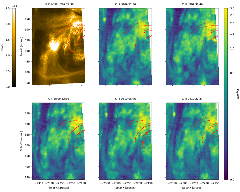
Figure 29: Same as in Figure 13 but for the C III line.

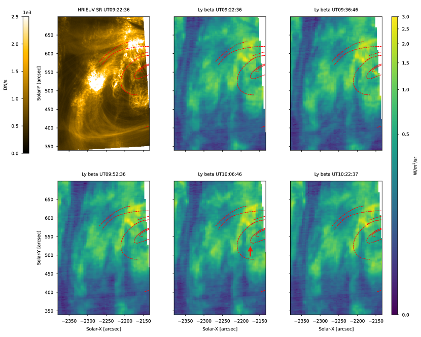
Figure 30: Same as in Figure 13 but for the Lyman-$\beta$ line.

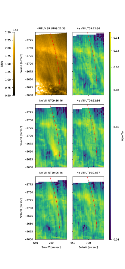
Figure 32: Same as in Figure 17 but for the Ne VIII line.

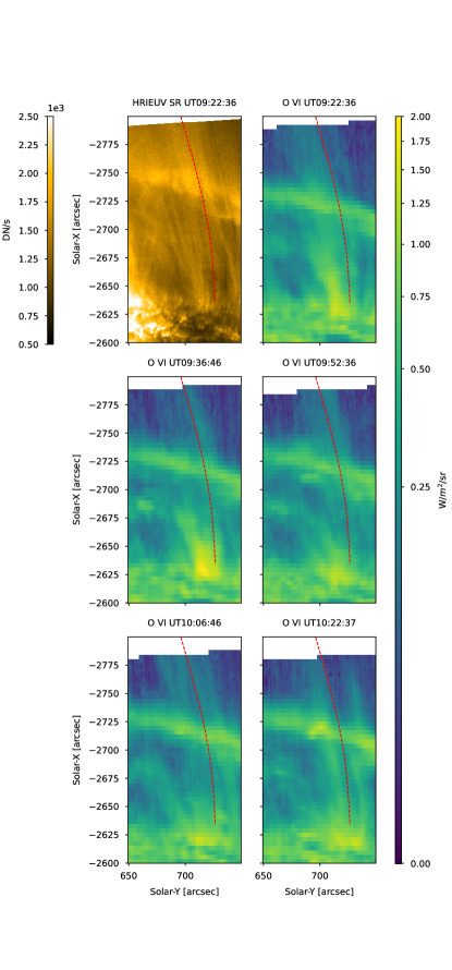
Figure 33: Same as in Figure 17 but for the O VI line.

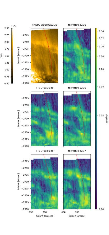
Figure 34: Same as in Figure 17 but for the N IV line.

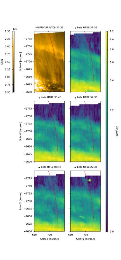
Figure 35: Same as in Figure 17 but for the Lyman-$\beta$ line.

Appendix B Time-distance diagrams with HRI_EUV on April 1