Abstract

Mass loss from massive stars plays a determining role in their evolution through the upper Hertzsprung-Russell diagram. The hydrodynamic theory that describes their steady-state winds is the line-driven wind theory (m-CAK). From this theory, the mass-loss rate and the velocity profile of the wind can be derived, and knowing these properly will have a profound impact on quantitative spectroscopy analysis from the spectra of these objects. Currently, the so-called $\beta$ law, which is an approximation for the fast solution, is widely used instead of the m-CAK hydrodynamics, and when the derived value is $\beta\gtrsim 1.2$, there is no hydrodynamic justification for these values. This review focuses on 1) a detailed topological analysis of the equation of motion (EoM); 2) solving numerically the EoM for all three different (fast and two slow) wind solutions; 3) deriving analytical approximations for the velocity profile via the Lambert$W$ function and 4) give a discussion of the applicability of the slow solutions.

1 1 0 https://doi.org/ Radiation-Driven Wind Hydrodynamics of Massive Stars: A Review Massive Stars Wind Hydrodynamics Michel Curé¹  and Ignacio Araya²   Michel Curé and Ignacio Araya Curé & Araya Correspondence: michel.cure@uv.cl

1 Introduction

At the beginning of the XX century, Johnson (1925, 1926) and Milne (1926) argued that the force on ions in the atmosphere of a luminous star could be responsible for the ejection of these ions from the star. They also argued that the ejected ions should carry with them the corresponding number of electrons, strictly there should be no charge–current, but they did not realize at that time that the collisional coupling between ions and protons would drag the rest of the plasma (mostly fully ionized Hydrogen), with them as well, at least to supersonic velocities, and this theory was laid aside. It was Chandrasekhar Chandrasekhar (1941, 1943), who in the context of globular cluster dynamics, developed the theory of collisions due to an inverse square law, and Spitzer (1956) applied Chandrasekhar’s theory for collisions between charged particles.

Morton (1967) was the first to report far-ultraviolet observations of three OB supergiants from an Aerobee-sounding rocket. After this came Copernicus, the first satellite with a telescope on board, and since then it has been possible to obtain stellar spectra in the ultraviolet (UV) region. Morton (1967) found that the resonance lines of C IV, N V and Si IV showed the typical P-Cygni profiles. He found that the displacements in the profiles of C IV $\lambda\lambda 1549.5$ and Si IV $\lambda\lambda 1402.8$ corresponding to outflow velocities in the range 1500–3000 km/s.

Snow and Morton (1976) showed through a detailed survey that stars brighter than $M_{bol}\sim-6$ have strong P-Cygni profiles in their spectra and therefore lose mass. The same conclusion was arrived at by Abbott (1982), who compared the radiative force with the gravitational force and concluded that radiative forces could initialize and maintain the mass-loss process for stars with an initial mass at the zero-age main sequence (ZAMS) of about 15 $M_{\odot}$ or greater.

This mass-loss process (known as stellar wind), together with supernovae explosions, are the main contributors in supplying the interstellar medium (ISM) with nuclear-processed heavy elements and therefore influence not only the chemical evolution (and therefore star formation) but also the energy equilibrium of the ISM and the Galaxy (see Kudritzki and Puls, 2000; Puls et al., 2008; Vink, 2022, and references therein).

Parker (1958) was the first to develop the solar wind through a purely gas-dynamical theory, which was until the winds of massive stars were discovered, the only known stellar wind theory. When this theory was applied to the winds of a typical O-star, the effective temperature necessary to reproduce the observed terminal velocities was of the order of $10^{7}$ K, a value that is completely excluded by the presence of lines such as Si IV, C IV and N V ions, which would be destroyed by collisional ionization at temperatures above $3\times 10^{5}$ K. It was, therefore, necessary to seek an alternative mechanism to drive the wind. The natural driven mechanism is the force due to the interaction of the radiation field on the wind plasma, and the simplest form is the force due to the continuum, i.e., the Thompson radiative acceleration. This force leads macroscopically to a decrease in the star’s gravitational attraction by a constant factor (for O–stars between $0.3$ and $0.6$). It is then clear that the continuum force alone cannot produce a force that exceeds gravity and, therefore, cannot drive these kinds of winds.

Lucy and Solomon (1970) resuscitated the proposal of Johnson and Milne and considered the force due to the absorption of spectral lines, but unlike the earlier authors, they considered the flow of the plasma as a whole rather than the selective ejection of specific ions. They calculated an upper limit on the force on the C IV line $\lambda\lambda 1548$ finding that this exceeds the force of gravity by a factor of approximately a few hundred. Hydrostatic equilibrium in the outermost layers is not possible, and an outflow of material must occur. In their stellar wind model, Lucy and Solomon made a series of assumptions, for instance, that the wind is driven only by resonance lines. They found mass-loss rates for O-stars of two orders of magnitudes less than the values obtained from observations.

A significant step in the theory was made by Castor, Abbot & Klein Castor et al. (1975) (hereafter CAK), who realized that the force due to line absorption in a rapidly expanding envelope could be calculated using the Sobolev approximation (Sobolev, 1960; Castor, 1974). Then by developing a simple parameterization of the line force, using the point star approximation, they were able to construct an analytical wind model. Despite the number of approximations made in that work, e.g., they represented the line force by C III lines and calculated only one model for a typical O5 f star ($T_{\rm{eff}}=49\,290$ K, $\log g=3.94$ and $R/R_{\odot}=13.8$) obtaining a mass-loss rate $\dot{M}=6.61\times 10^{-6}\,M_{\odot}/$year and a terminal velocity $v_{\infty}=1515\,$ km/s. The value of the mass-loss rate was of the same order of magnitude as the values obtained from observation, but the terminal velocity lay below the measured ones. They also gave analytical scaling relations for the mass-loss rates and terminal speeds as functions of the stellar parameters. These were widely used to prove (or disprove) the validity of the radiation-driven (or line-driven) wind theory by comparison with the observations.

Abbott (1982) improved this theory by calculating the line force using a tabulation of ca. $250\,000$ lines, which was complete for the elements H to Zn in the ionization states I to VI. Currently, the non-local thermodynamic equilibrium code CMFGEN (Hillier, 2012) uses around $900\,000$ lines; or FASTWIND with 4 million lines Pauldrach et al. (2001) (see also Lattimer and Cranmer, 2021, who used ca. 4 million lines). Despite this immense effort to give a more realistic representation of the line force, evident discrepancies with the observations remained. Simultaneously and independently, Friend and Abbott (1986) and Pauldrach et al. (1986) (hereafter FA and PPK, respectively) calculated the influence of the finite cone angle correction on the dynamics of the wind (described in the appendix from Castor, 1974). They found a much better agreement between the improved or modified CAK theory (hereafter m-CAK) and the observations for the mass loss rate and the terminal velocity in a large domain in the Hertzsprung-Russell diagram.

The equation of motion of the m-CAK theory is a highly non-linear differential equation that has singular points, eigenvalues and solution branches (see Castor et al., 1975; Friend and Abbott, 1986; Pauldrach et al., 1986; Bjorkman and Carciofi, 2005; Curé and Rial, 2007; Curé et al., 2011). Since it is challenging to solve this differential equation numerically, PPK found that the velocity field, $v(r)$ from the m-CAK theory, can be described by a simple approximation, known as the $\beta$ law approximation (see below). In addition, Kudritzki et al. (1989, hereafter KPPA) developed analytical approximations for the localization of the critical point, mass loss rate and terminal velocity with an agreement within 5% for $v_{\infty}$ and 10% for $\dot{M}$, when compared to the correct numerical calculations.

Radiation-driven stellar winds are hydrodynamic phenomena involving the flow of the outer layers of the atmospheres of massive stars. This review is focused on describing the investigation of the m-CAK hydrodynamic theory, its topology and its three known physical solutions.

Section 2 presents the theory to calculate the radiation (line) force via an analytical description thanks to the Sobolev approximation. Section 3 introduces the m-CAK hydrodynamic theory, and its topological description is given in section 4. Section 5 shows all three known physical solutions, whilst section 6 present analytical approximate solutions based on the Lambert$W$ function. Finally, in section 7, we summarise the main topics of this review and discuss the applicability of slow solutions.

2 The Radiation Force

The exact calculation for the radiation force requires a knowledge of the radiation field (in all the lines and continua) and of the physical processes (scattering, absorption and emission) that contribute to the exchange of energy and momentum throughout the wind. The radiation field is represented by the monochromatic specific intensity $I_{\nu}(\mu)$, $\mu$ is the cosine of the angle between the incoming beam and the velocity vector of the interacting particles. Thus, the radiation force per unit of volume, at a distance r, exerted on a point particle per unit of time is equal to momentum removed from the incident radiation field ($\kappa\rho\,I(\mu)\,\mu/c$) integrated over all the scattering directions. This force is given by

$${\bf{F}}^{\rm{rad}}(r)=\frac{4\pi}{c}\frac{1}{2}\int_{0}^{\infty}\int_{-1}^{1}\>\kappa_{\nu}(r)\,\rho(r)\,I_{\nu}\,\mu\,d\!\mu\,d\!\nu,$$ (1)

where the absorption coefficient $\kappa_{\nu}$ is given in units of cm² g^-1. The net flux density comes from the interaction processes, integrated over the whole spectral range, between the radiation field emitted by the photosphere and the stellar wind of mass density $\rho$ at the distance $r$. Here, it is assumed that the emissivity (thermal emission and photon scattering) in the expanding atmosphere is isotropic. Therefore, no net momentum change occurs from this process (see Hubeny and Mihalas (2015), Chapter 20).

The absorption coefficient $\kappa_{\nu}$ consists of three main contributions:

$$\kappa_{\nu}=\kappa^{\rm{Th}}+\kappa_{\nu}^{\rm{cont}}+\kappa_{\nu}^{\rm{line}},$$ (2)

where $\kappa^{\rm{Th}}$ represents the Thomson scattering, $\kappa_{\nu}^{\rm{cont}}$ the contribution of bound-free and free-free transitions and $\kappa_{\nu}^{\rm{line}}$ the sum of all line absorption coefficients at frequency $\nu$.

The radiation force can be calculated by state-of-the-art non-local thermodynamic equilibrium (NLTE) radiative transfer codes such as Fastwind Santolaya-Rey et al. (1997); Puls et al. (2005), Cmfgen Hillier (1987); Hillier and Miller (1998); Hillier and Lanz (2001); Hillier (2012) or PoWR Hamann and Schmutz (1987); Todt et al. (2015), but these calculations depend on the velocity and density profile used to describe the wind.

2.1 Radiative force due to electron scattering

The interaction between photons and free electrons is described by a Compton process (an excellent review of this process, including Monte-Carlo calculations can be found in Pozdnyakov et al. (1983)). If photons with energy $h\nu\ll m_{e}c^{2}$ are scattered by Maxwellian electrons having $kT\ll m_{e}c^{2}$, the frequency shift will be very small, but if the scattering process is repeated many times, the small amounts of energy exchanged between the electrons and photons can build up and give rise to substantial effects.

In the non-relativistic limit without the influence of quantum effects ($h\nu\ll m_{e}c^{2}$), and neglecting the possible effects described above, the scattering cross-section is frequency-independent and called the Thomson cross-section, namely:

$$\sigma^{\rm{Th}}=\frac{8\pi}{3}\frac{e^{4}}{m_{e}^{2}c^{4}}.$$ (3)

The value of this cross-section is $\sigma^{\rm{Th}}=6.65\times 10^{-25}\,\mathrm{cm^{2}}$ and the absorption coefficient is, therefore:

$$\kappa^{\rm{Th}}\rho\,=n_{e}\,\sigma^{\rm{Th}}.$$ (4)

Using this value ($\kappa^{\rm{Th}}$) in Eq. (2) and integrating Eq. (1), we obtain the contribution of the Thomson scattering to the radiation force,

$${\bf{F}}^{\rm{Th}}=n_{e}\frac{\sigma^{\rm{Th}}\,L}{4\pi c\,r^{2}}\,,$$ (5)

where $L$ is the luminosity of the star. The radiative acceleration on the electrons is then

$$g_{e}^{\rm{Th}}=\frac{1}{m_{e}}\frac{\sigma^{\rm{Th}}\,L}{4\pi cr^{2}}.$$ (6)

It is useful to define the ratio of the Thomson scattering force and the gravitational force by:

$$\Gamma_{e}=\frac{g_{e}^{\rm{Th}}}{g^{\rm{grav}}}=\frac{1}{m_{e}}\frac{\sigma^{\rm{Th}}\,L}{4\pi\,c\,GM_{*}}\,,$$ (7)

here $G$ is the gravitational constant and $M_{*}$ the star’s mass. In the standard one-component description of stellar winds, the force over the density of the plasma is given by:

$$g^{\rm{Th}}=\left(\frac{n_{e}}{\rho}\right)\frac{\sigma^{\rm{Th}}\,L}{4\pi c\,r^{2}}$$ (8)

being $\rho=m_{p}n_{p}+\sum_{\rm{ions}}(m_{i}n_{i})+n_{e}m_{e}$ the mass density. The principal contribution of the ions comes from Helium, and neglecting the electrons, $n_{e}m_{e}$, the density is

$$\rho\simeq m_{p}n_{p}(1+A_{\rm{He}}Y_{\rm{He}})\,.$$ (9)

Here $A_{\rm{He}}$ is the atomic mass of a Helium atom, $Y_{\rm{He}}$ is the relative abundance by number of Helium with respect to Hydrogen (the latter being described by the subscript $p$), and $m_{p}$ is the proton mass. Based on the conservation of charge, it is possible to express the electron number density as $n_{e}=n_{p}(1+q_{\rm{He}}Y_{\rm{He}})$, where $q_{\rm{He}}=0,1,2$ depending on the Helium ionisation state.

Thus, the ratio $n_{e}/\rho$ is:

$$\frac{n_{e}}{\rho}=\frac{1}{m_{p}}\left(\frac{1+q_{\rm{He}}Y_{\rm{He}}}{1+A_{\rm{He}}Y_{\rm{He}}}\right)$$ (10)

and the acceleration is:

$$g^{\rm{Th}}=\frac{1}{m_{p}}\left(\frac{1+q_{\rm{He}}Y_{\rm{He}}}{1+A_{\rm{He}}Y_{\rm{He}}}\right)\left(\frac{\sigma^{\rm{Th}}L}{4\pi c\,r^{2}}\right)$$ (11)

or

$$\Gamma_{e}=\left(\frac{1+q_{\rm{He}}Y_{\rm{He}}}{1+A_{\rm{He}}Y_{\rm{He}}}\right)\left(\frac{\sigma^{\rm{Th}}\,L}{4\pi\,c\,m_{p}\,GM_{*}}\right)$$ (12)

Quite often, the canonical value of $\kappa^{\rm Th}=0.34$ cm² g^-1 is adopted, which follows from assuming a fully ionised plasma at solar abundance. In addition, since the continuum of OB stars, near its maximum, is also optically thin in the lines, the contribution of the continuum to the total radiative force is neglected.

The next section provides a general description of the line force based on the Sobolev approximation (see, e.g., Lamers and Cassinelli (1999) or Hubeny and Mihalas (2015)).

2.2 Radiative force due to lines.

The contribution to the radiation force due to the spectral lines in the wind of massive stars is provided by the momentum transfer of photons (via absorption and re-emission processes in optically thick lines) mainly from the most dominant ions (i.e., C, O, N, and the Fe-group). The proper calculation of the line force (per unit volume) is given by:

$$F^{\rm{line}}(r)=\frac{2\pi}{c}\,\sum_{l}\int_{0}^{\infty}\int_{-1}^{+1}\kappa_{l}(r)\,\rho(r)\,\phi_{l}(\nu,\mu,r)\,I_{\nu}(r,\mu)\,\mu\,d\mu\,d\nu.$$ (13)

where $\phi$ is the Gaussian absorption profile. The summation is over all the line transitions ($l$), assuming non-overlapping lines, for which the wind is optically thick. $\kappa_{l}$ is the opacity coefficient (in cm² g^-1) of lines formed between levels $l$ (lower) and $u$ (upper) with energy h $\nu_{0}$,

$$\kappa_{l}\,\rho\,=\frac{\pi\,e^{2}}{m_{e}\,c}\,f_{l}\,n_{l}\,\left(1-\frac{n_{u}\,g_{l}}{n_{l}\,g_{u}}\right).$$ (14)

The number density $n_{l}$ and $n_{u}$ of ions in levels $l$ and $u$ are given in cm^-3, $g_{l}$ and $g_{u}$ are the corresponding statistical weights, and $f_{l}$ is the oscillator strength of the line. The CAK theory allows us to find an analytical expression for the line force in a moving media with large velocity gradients in terms of the macroscopic variables using the Sobolev approximation. However, this expression only applies to radiating flows in the non-relativistic regime.

2.2.1 The Sobolev approximation

In a moving plasma like the stellar wind, the interaction of radiation with matter can be better understood as follows. Let’s consider a single spectral line thermally broadened with a rest wavelength $\lambda_{1}$. A photon emitted from the stellar surface, with wavelength $\lambda_{\ast}<\lambda_{1}$, propagates without interacting with the matter until, due to the Doppler shift, it is scattered at the blue edge of the line in question. Due to the expansion of the wind, the particles viewed from any direction from a certain position always appear to be receding. This means that independent of the scattered direction of the photon (forward or backwards), the distance travelled always causes its comoving wavelength to be red-shifted.
After many scatterings, the photon’s wavelength has been shifted to the line’s red edge, and the interaction of this photon with the line ($\lambda_{1}$) ceases. The region in the wind where an incoming photon can interact with the ions is called the interaction zone. It is also well known that the winds of massive stars reach terminal velocities of several times the sound speed, and the point at which the wind velocity is equal to the sound speed (the sonic point) is very near to the photosphere. This means that almost all the region where stellar winds are found is supersonic.
This description corresponds to the Sobolev approximation (Sobolev, 1960), where all the relevant physical quantities, such as the opacity, source function, etc., are considered constant in the interaction zone, i.e., the width of the interaction zone is small compared with a characteristic flow length. Thus, for a generic Doppler-broadened line profile, the Sobolev-length, $L_{s}$, is defined as:

$$L_{s}=v_{\rm{th}}/(dv/dr),$$ (15)

where $T_{\rm{eff}}$ is the star’s effective temperature, $v_{th}=\sqrt{2\,k_{B}\,T_{\rm{eff}}/m_{p}}$ the thermal speed of the protons, $k_{B}$ the Boltzmann constant.

A characteristic length of the flow is

$$L_{c}\simeq v/(dv/dr)$$ (16)

Typical values of thermal velocities in OB-types stars are about $7-20$ km/s while terminal velocities are about $1000$-$3000$ km/s, (see, e.g., Lamers and Cassinelli (1999); Puls et al. (2008)). More recent measurements of terminal velocities based on observations performed in the frame of the ULLYSES collaboration (Roman-Duval et al., 2023) have been accomplished by Hawcroft et al. (2023).

2.2.2 The line-force due to a single-line

Castor (1974) analysed in detail the Sobolev approximation in the context of stellar winds and showed that the force produced by the incoming radiation due to a single line can be expressed as:

$$f^{\rm{line}}=\left(\frac{F_{\nu}\,\Delta\nu_{d}}{c}\right)\left(\frac{k_{l}}{\tau_{l}}\right)(1-e^{-\tau_{l}}),$$ (17)

where $\Delta\nu_{d}=v_{\rm{th}}\,\nu/c$ corresponds to the Doppler shift, $F_{\nu}$ is the flux of the radiation field at frequency $\nu$, $k_{l}$ is the monochromatic line absorption coefficient per unit mass, and

$$\tau_{l}=\int\rho\,\phi(\nu,r)\,k_{l}\,dr$$ (18)

is the optical depth. Evaluating the optical depth for a normalized Gaussian profile and using the Sobolev approximation, we find:

$$\tau_{l}=k_{l}\,\rho\,v_{\rm{th}}/(dv/dr).$$ (19)

With this expression, we can interpret the RHS of (17) as:

• $(F_{\nu}\,\Delta\nu_{d}/c)$ is the rate of momentum emitted by the star per unit area at frequency $\nu$ with bandwidth $\Delta\nu_{d}$,

• $(\tau_{l}/k_{l})=\rho\,v_{\rm{th}}/(dv/dr)$ represents the amount of mass that can absorb this momentum, and

• $(1-e^{-\tau_{l}})$ is the probability that such an absorption occurs.
  

Then, by defining,

$$t=\sigma_{e}\,\rho\,v_{\rm{th}}/(dv/dr)\,,$$ (20)

where $\sigma_{e}=\sigma^{\rm{Th}}n_{e}/\rho$ corresponds to the Thomson scattering absorption coefficient per density. In a moving medium, $t$ represents the optical depth that a line will have if its opacity is equal to its electron scattering opacity. Based on this definition, it is possible to rewrite $t$ as

$$\tau_{l}=\eta_{l}\,t$$ (21)

where $\eta_{l}=k_{l}/\sigma_{e}$. The first factor in (21) is related only to line properties, and the second only to dynamic variables of the wind.

2.2.3 The line-force due to a statistical distribution of line strength

The total line force, due to the addition of all the single lines of the ions, for a point star approximation and for non-overlapping single lines, is given by:

$$f^{\rm{line}}=\sum_{l}\left({\frac{F_{\nu}\Delta\nu_{d}}{c}}\right)_{\!l}\,\left({\frac{dv/dr}{\rho\,v_{\rm{th}}}}\right)\,(1-e^{-\eta_{l}t}).$$ (22)

Expressing (22) in terms of $\Delta\nu_{d}=\nu\,v_{\rm{th}}/c$, and the relation, $F=L/4\pi r^{2}$, we obtain

$$f^{\rm{line}}=\frac{L}{c^{2}}\left(\frac{dv/dr}{4\pi r^{2}}\right)\,\sum_{l}\left({\frac{L_{\nu}\,\nu}{L}}\right)_{\!l}(1-e^{-\eta_{l}t})$$ (23)

Abbott (1982) was the first to compile and publish a list of ca. 250 000 lines for atoms from H to Zn in ionisation stages I to VI. Based on such a line list (Hillier and Miller, 1999; Noebauer and Sim, 2015; Lattimer and Cranmer, 2021), it is possible to derive a line strength distribution function (Pauldrach et al., 1986; Puls et al., 2000). This distribution can be described as follows:

$$dN(k_{l})=\int_{0}^{N}\left(\frac{L_{\nu}\,\nu}{L}\right)\,n(k_{l},\nu)d\nu$$ (24)

and represents the number of lines in the line-strength interval $(k_{l},k_{l}+\Delta k_{l})$ obtained from the total spectrum and weighted by the flux mean of line strength $(L_{\nu}\,\nu/L)$. Notice that in Eq. (24) the distribution in frequency space of the lines is independent from the distribution in line strength. An alternative formulation of the line statistic is given by Gayley (1995) (see also Lattimer and Cranmer, 2021).

The logarithm of the number of lines can be fitted by a linear function, namely:

$$dN(k_{l})=N_{0}\,(1-\alpha)\,{\left(k_{l}/\sigma_{e}\right)}^{\alpha-2}\,d\left(k_{l}/\sigma_{e}\right)$$ (25)

being $N_{0}$ the number of lines (strong and weak) that effectively contribute to the line force. Typical values of the parameter $\alpha$ are $0.45\leq\alpha\leq 0.7$ (Lamers and Cassinelli, 1999; Puls et al., 2000). Notice that line force parameters are not free but depend on the transfer problem in each individual star (see Puls et al., 2000; Noebauer and Sim, 2015; Gormaz-Matamala et al., 2019; Lattimer and Cranmer, 2021; Gormaz-Matamala et al., 2021; Poniatowski et al., 2022, for a detailed description of the calculation of the line-force parameters).

Extending the sum in Eq. (23) to an integral, we obtain the line force expression:

$$f^{\rm{line}}=\frac{L}{c^{2}}\,\frac{(dv/dr)}{4\pi r^{2}}\,N_{0}\,(1-\alpha)\,\int_{\sigma_{e}}^{\infty}(1-e^{-\eta_{l}t}){\left(k_{l}/\sigma_{e}\right)}^{(\alpha-2)}\,d\left(k_{l}/\sigma_{e}\right).$$ (26)

Neglecting the lower limit of the integral, a valid approximation for stars of type OB, replacing it by zero and integrating, the line force becomes:

$$f^{\rm{line}}=\frac{L}{c^{2}}\,\frac{1}{4\pi r^{2}}\,v_{\rm{th}}\,\sigma_{e}\,N_{0}\,(1-\alpha)\,\Gamma\!(\alpha){\left(\frac{dv/dr}{\sigma_{e}\,\rho\,v_{\rm{th}}}\right)}^{\alpha},$$ (27)

where $\Gamma$ is the $\Gamma$-function. Then, dividing by the total density, we obtain the standard form of the line acceleration,

$$g^{\rm{line}}=\frac{C}{r^{2}}{\left(r^{2}\,v\,\frac{dv}{dr}\right)}^{\alpha}\,,$$ (28)

with

$$C=\Gamma_{e}\,GM_{*}\,k{\left(\frac{4\pi}{\sigma_{e}\,v_{\rm{th}}\,\dot{M}}\right)}^{\alpha}\,,$$ (29)

here, $\Gamma_{e}$ is the radiative acceleration due to Thomson scattering in terms of the gravitational acceleration, and $\dot{M}$ is the mass-loss rate. Here the continuity equation has been used, and the variables, such as $N_{0}$ or $\Gamma(\alpha)$, have been collected into the constant $k$. Note that this expression for the line-force (Eq. 28) only takes interactions between ions and radially emitted photons into account (Castor, 1974; Castor et al., 1975).

2.2.4 The correction factor

CAK (see their appendix) discussed qualitatively the effect on the line force that the proper shape of the star (non-radial incoming photons) would have on the wind kinematics. Later PPK and FA independently investigated the influence of this effect, known as the finite disk correction factor, thereby developing the m-CAK theory.

The expression of the line force for incoming photons from an arbitrary direction, for a radial flow velocity field, comes from the definition of Eq. (20), thus,

$$t_{\sigma}=\left(\frac{1+\sigma}{1+\mu^{2}\sigma}\right)\frac{\sigma_{e}\,\rho\,v_{\rm{th}}}{dv/dr},$$ (30)

where

$$\sigma=\frac{d\ln v}{d\ln r}.$$ (31)

Inserting $t_{\sigma}$ in Eq. (26), instead of $t$, and integrating, we obtain the following expression for the line force:

$$g^{\rm{line}}=\frac{C}{r^{2}}CF(r,v,v^{\prime}){\left(r^{2}\,v\,v^{\prime}\right)}^{\alpha}$$ (32)

where $CF$ is the correction factor, defined as the ratio of the force due to the non-radial contributions to that of a point star approximation, namely:

$$CF=\frac{2}{1-\mu_{c}^{2}}\int_{\mu_{c}}^{1}{\left[\frac{(1-\mu^{2})\,v/r+\mu^{2}v^{\prime}}{v^{\prime}}\right]}^{\alpha}\,\mu\,d\mu$$ (33)

here $\mu_{c}=\sqrt{(1-R_{\ast}^{2}/r^{2})}$, where $R_{\ast}$ is the stellar radius, and $v^{\prime}=dv/dr$. In appendix A, we summarised some properties of the correction factor.

2.3 The Ionization Balance

In his work, Abbott (1982), assumed local thermodynamic equilibrium (LTE) and used the modified Saha formula (see Hubeny and Mihalas (2015)) to take into account the dilution of the radiation field and the possible difference between the electron kinetic temperature $T_{e}$ and the radiation temperature $T_{r}$. Due to the changes in the ionisation throughout the wind, Abbott fitted the line force not only in terms of $(r^{2}\,v\,v^{\prime})^{\alpha}$ (see Eq. 28) but also as a function of the ratio $n_{e}/W(r)$, where

$$W(r)=\frac{1}{2}\left(1-\sqrt{(1-R_{\ast}^{2}/r^{2})}\right)\,,$$ (34)

is the dilution factor. He found that the functional dependence of this quotient in the line force is:

$$g^{\rm{line}}\propto{\left(\frac{n_{e}}{W(r)}\right)}^{\delta},$$ (35)

where the electron number density, $n_{e}$, is given in units of $10^{11}\rm{cm^{-3}}$. This proportionality means that the greater the density, the lower the ionisation level. In view of the fact that the lower ionisation levels have more line transitions, usually at the maximum of the radiation field, the line force increases with increasing density. Values of this $\delta$ line-force parameters for the fast solution (see below) are in the range $0<\delta\lesssim 0.2$ (Lamers and Cassinelli, 1999), but for a pure Hydrogen atmosphere, the value is $\delta=1/3$ as Puls et al. (2000) demonstrated.

3 The m-CAK Hydrodynamic model

The 1-D m-CAK stationary model for line-driven stellar winds considers the following assumptions: an isothermal fluid in spherical symmetry and neglecting the influence of viscosity effects, heat conduction and magnetic fields.

The stationary continuity and momentum conservation equations are:

$$\dot{M}=4\,\pi\,r^{2}\,\rho\,v,$$ (36)

$$v\,\frac{dv}{dr}=-\frac{1}{\rho}\,\frac{{dP}}{dr}-\frac{GM_{*}(1-\Gamma_{e})}{r^{2}}+\frac{v_{\phi}^{2}(r)}{r}+g^{\rm{line}}(\rho,dv/dr,n_{e}),$$ (37)

being $P$ the fluid pressure, $v_{\phi}=v_{rot}R_{\ast}/r$, where $v_{rot}$ is the stellar rotational speed at the equator. In addition, $g^{\rm{line}}(\rho,dv/dr,n_{e})$ corresponds to the acceleration due to an ensemble of lines.

The standard or m-CAK parameterization of the line force Abbott (1982); Pauldrach et al. (1986); Friend and Abbott (1986) is the following:

$$g^{\rm{line}}=\frac{C}{r^{2}}\;CF(r,v,dv/dr)\;\left(r^{2}v\frac{dv}{dr}\right)^{\alpha}\;\left(\frac{n_{e}}{W(r)}\right)^{\delta},$$ (38)

where the coefficient $C$ is given by Eq. (29).

Substituting the density from the mass conservation equation (Eq. 36) into the momentum equation (Eq. 37), we obtain the equation of motion (EoM).

Transforming to dimensionless variables, that is:

$$u = -\frac{R_{\ast}}{r}\,,$$ (39)

$$w = \frac{v}{a}\,,$$ (40)

$$w^{\prime} = \frac{dw}{du}\,,$$ (41)

where $a$ is the isothermal sound speed of an ideal gas, $P=a^{2}\rho$.

Using these new variables, the EoM now reads:

$$F(u,w,w^{\prime})=\left(1-\frac{1}{w^{2}}\right)w\frac{dw}{du}+A+\frac{2}{u}+a_{\rm{rot}}^{2}u-C^{\prime}\;CF\;g(u)(w)^{-\delta}\left(w\frac{dw}{du}\right)^{\alpha}\ =0\,,$$ (42)

where the constants are the following:

$$A = \frac{GM(1-\Gamma_{e})}{a^{2}R_{\ast}}=\frac{v_{\rm{esc}}^{2}}{2a^{2}},$$ (43)

$$a_{\rm{rot}} = \frac{v_{\rm{rot}}}{a},$$ (44)

$$C^{\prime} = C\;\left(\frac{\dot{M}D}{2\pi}\frac{10^{-11}}{aR_{\ast}^{2}}\right)^{\delta}\;(a^{2}R_{\ast})^{(\alpha-1)},$$ (45)

$$D = \frac{(1+Z_{\rm{He}}Y_{\rm{He})}}{(1+A_{\rm{He}}Y_{\rm{He}})}\frac{1}{m_{\rm{p}}},$$ (46)

being $Z_{\rm{He}}$ the number of free electrons provided by Helium, $v_{\rm{esc}}$ the escape velocity, and the function $g$ is defined as:

$$g(u)=\left(\frac{u^{2}}{1-\sqrt{1-u^{2}}}\right)^{\delta}$$ (47)

In order to find a physical wind solution of the EoM (Eq. 42), i.e., starting from the photosphere with a small velocity and reaching infinite with a supersonic velocity, we first need to understand the topology of this equation.

4 Topological Analysis

As mentioned previously, the first wind model was developed by Parker (1958) for the sun. This model possesses a singular point at the sonic point and different solution branches (see Fig. 3.1 from Lamers and Cassinelli, 1999). The m-CAK model has a driving force (line force) that depends not only on the radial coordinate $r$ (or $u$) but also on the velocity and the velocity gradient. These characteristics complicate the study of the EoM’s topology that gives rise to the different solutions.

Mathematically, singular points are located where the singularity condition is satisfied, i.e.:

$$\frac{\partial}{\partial w^{\prime}}F(u,w,w^{\prime})=0\,,$$ (48)

and these locations form the locus of singular points.

At these specific points, in order to have a smooth wind solution between solution branches, a regularity condition must be imposed, namely:

$$\frac{d}{du}F(u,w,w^{\prime})=\frac{\partial F}{\partial u}+\frac{\partial F}{\partial w}w^{\prime}=0$$ (49)

Using the following coordinate transformation:

$$Y=w\;w^{\prime}$$ (50)

$$Z=w/w^{\prime},$$ (51)

we can now solve Equations (42), (48) and (49), only valid simultaneously at one singular point, obtaining the following set of Equations:

$$Y-\frac{1}{Z} +A+2/u+a_{rot}^{2}u -\,C^{\prime}f_{1}(u,Z)\,g(u)\,Z^{-\delta/2}\,Y^{\alpha-\delta/2}=0\;,$$ (52)

$$Y-\frac{1}{Z} -\,C^{\prime}f_{2}(u,Z)\,g(u)\,Z^{-\delta/2}\,Y^{\alpha-\delta/2}=0\;,$$ (53)

$$Y+\frac{1}{Z} -2Z/u^{2}+a_{rot}^{2}Z\ -\,C^{\prime}f_{3}(u,Z)\,g(u)\,Z^{-\delta/2}\,Y^{\alpha-\delta/2}=0\;,$$ (54)

derivation details and definitions of $f_{1}(u,Z)$, $f_{2}(u,Z)$ and $f_{3}(u,Z)$ are summarised in appendix B.

Solving for $Y$ and $C^{\prime}$ from the set of Equations (52), (53) and (54), we obtain:

$$Y=\frac{1}{Z}+\left(\frac{f_{2}(u,Z)}{f_{1}(u,Z)-f_{2}(u,Z)}\right)\times\left(A+\frac{2}{u}+a_{rot}^{2}u\right)$$ (55)

and

$$C^{\prime}(\dot{M})=\frac{1}{gf_{2}}\left(1-\frac{1}{Y\,Z}\right)\;Z^{\delta/2}\;Y^{1-\alpha+\delta/2}$$ (56)

These last two Eqs. are generalisations of the relations found by KPPA (see their Eq.[21] and Eq.[34] for $Y$ and Eq.[20] and Eq.[44] for the eigenvalue), but now including the rotational speed of the star.

4.1 The critical point function $R$

The set of Eqs. (52), (53) and (54) are only valid at the singular point for the unknowns: $Y_{s}$, $C^{\prime}_{s}$, $Z_{s}$ and $u_{s}$. Due to the fact that there are only three equations and four unknowns, it is not possible to solve them. Nevertheless, from this set of Equations, we can derive the function, $R(u,Z)$, defined by:

$$R(u,Z)=-\frac{2}{Z}+\frac{2Z}{u^{2}}-a_{\rm{rot}}^{2}Z+f_{123}(u,Z)\left(A+\frac{2}{u}+a_{\rm{rot}}^{2}u\right)$$ (57)

where $f_{123}(u,Z)$ has the following definition:

$$f_{123}(u,Z)=\frac{f_{2}(u,Z)-f_{3}(u,Z)}{f_{2}(u,Z)-f_{1}(u,Z)}$$ (58)

The locus of singular points, $u_{s}$, is given by the points which are solutions of the following equation:

$$R(u,Z)=0\,.$$ (59)

It should be noted that no approximation has been made in the derivation of the above topological equations.

To determine which is the location of the singular point in the locus of points that satisfies, $R(u,Z)=0,$ and therefore determine the values of $Y_{s}$,$C^{\prime}_{s}$, $Z_{s}$ and $u_{s}$, we need to set a boundary condition at the stellar surface.
For this boundary condition, the most used are:

• Set the density at the stellar surface to a specific value,

  $$\rho(R_{*})=\rho_{*},$$ (60)

  Usually this base density is in the range $10^{-8}\,\rm{g\,cm^{-3}}$ to $10^{-13}\,\rm{g\,cm^{-3}}$. For some examples, see the works of de Araujo and de Freitas Pacheco (1989); Friend and MacGregor (1984); Madura et al. (2007); Curé (2004); Araya et al. (2018).

• Set the optical depth integral to a specific value, i.e.,

  $$\tau_{*}=\int_{R_{\ast}}^{\infty}\sigma_{E}\,\rho(r)dr=\frac{2}{3}.$$ (61)

Employing one of these boundary conditions at the stellar surface plus the regularity condition at the singular point, we can solve from the EoM (Eq. 42) the velocity profile, $w=w(u)$, together with the value of the eigenvalue, $C^{\prime}$, and therefore the mass loss rate, $\dot{M}$.

5 Types of solutions

We developed a numerical code that discretizes by finite differences the EoM and, using the Newton-Raphson method, iterates to a numerical solution, this code is called Hydwind and is described in more detail in Curé (2004) (see also Curé, 1992).

After performing the topological analysis of the EoM, we were able, thanks to Hydwind, to find the numerical solutions of all three known m-CAK physical solutions: fast, $\Omega$-slow and $\delta$-slow solutions.

5.1 Fast solution

From the pioneering work of CAK and its improvements from FA and PPK, the code Hydwind is able to obtain the standard solution of the m-CAK theory, and we called it hereafter the fast solution.

To perform our topological analysis, we use a typical O5 V star with the following stellar parameters, $T_{\rm eff}=45000K$, $\log g=4.0$, $R/R_{\odot}=12$, and line force parameters $k=0.124$, $\alpha=0.64$, and $\delta=0.07$, with the boundary condition $\tau_{*}=2/3$.

The function $R(u,Z)$ is shown in Fig. 1 for a non-rotating star ($a_{\rm{rot}}=0$). The plane $R(u,Z)=0$ is plotted in light grey (right panel) and the intersection of both functions, which corresponds to the locus of singular points, is plotted with black lines. The locus of singular points for the fast solution is the one that starts at $Z\sim 0$ and $u=-1$. The other locus of singular points will be discussed below.

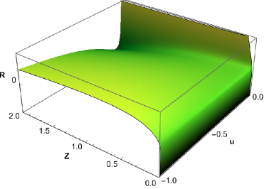
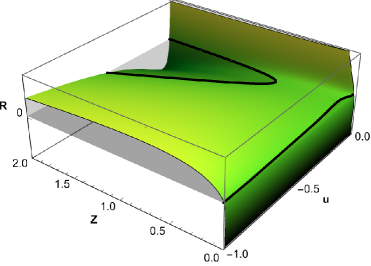
Figure 1: Function $R(u,Z)$ for a typical O5 V star without rotation. The left panel shows only the function $R(u,Z)$, while the right panel is similar to the left panel, but the plane $R(u,Z)=0$ is also plotted in light grey. Furthermore, the intersection of both curves (black solid lines) shows two locus of singular points.

Knowing the topology of the m-CAK model, specifically the locus of singular points, we now solve the EoM for the velocity profile, $v(r)$, or equivalently $w=w(u)$, and the eigenvalue $C^{\prime}$, which is proportional to the mass loss rate, $\dot{M}$. Then, the wind parameters obtained for this model are: a terminal velocity ($v_{\infty})$ of $3467\,{\rm km/s}$ and a mass-loss rate ($\dot{M}$) of $2.456\times 10^{-6}\,M_{\odot}/{\rm yr}$. Figure 2 shows the velocity profile of this model as a function of $\log(r/R_{*}-1)$ (left panel) and as a function of $u$ (right panel). The location of the singular point ($r_{s}$) is shown with a red dot, and it is located near the stellar surface ($r_{s}=1.029\,R_{*}$ or $u_{s}=-0.9719$). At this point, the wind velocity is $181.4\,\rm{km/s}$, a highly supersonic speed ($a=24.17\,\rm{km/s})$.

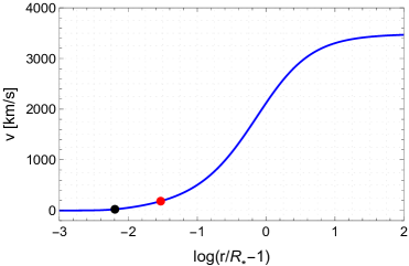
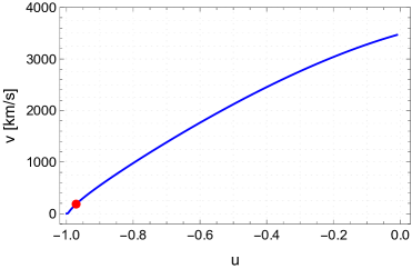
Figure 2: Velocity profile for a typical O5 V star without rotation. The velocity profile is plotted as a function of $\log(r/R_{\ast}-1)$ (left panel) and as a function of $u$ (right panel). The location of the singular point is shown with a red dot, while the sonic point is in black.

This steep velocity gradient is due to the rapid increase of the line force just above the stellar surface, as shown in Fig. 3, where the sound speed is reached at $r=1.006\,R_{*}$ and the maximum of $g^{\rm{line}}$ is reached at $r=1.3\,R_{*}$.

Figure 3: The radiative acceleration, $g^{\rm{line}}$, for a typical O5 V star without rotation as function of $r/R_{*}$, for $r<10\,R_{\ast}$.

As previously mentioned, the wind parameters ($v_{\infty}$ and $\dot{M}$) must be calculated within the framework of the radiative transport problem. However, to understand the complex non-linear dependence on the wind parameters from the line-force parameters, in the following figures, we show how the wind parameters depend in terms of each one of the line-force parameters.

Figure 4 shows the dependence of the wind parameters, $v_{\infty}$ (left panel) and $\dot{M}$ (right panel) as a function of the line force parameter $\alpha$, using the same stellar parameters and keeping the line force parameters $k$ and $\delta$ fixed. There is an increase in the values of both wind parameters as $\alpha$ increases.

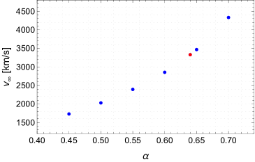
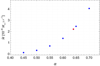
Figure 4: Dependence of the wind parameters as a function of the line-force parameter $\alpha$. Terminal velocity (left panel) and mass-loss rate (right panel). The values obtained for our typical O5 V star without rotation are shown in red.

The dependence of the wind parameters as a function of the line force parameter $k$ is shown in Fig. 5. In this case, wind parameters also increase as $k$ increases. It is clearly seen in Fig. 5 that the terminal velocity depends only slightly on the value of $k$ rather than the mass-loss rate, which has a significant impact on the value of $k$ (Venero et al., 2016).

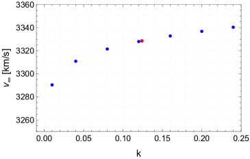
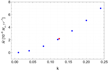
Figure 5: Dependence of the wind parameters as a function of the line-force parameter $k$. Terminal velocity (left panel) and mass-loss rate (right panel). The values obtained for our typical O5 V star without rotation are shown in red.

Finally, the dependence of the wind parameters as a function of the line force parameter $\delta$ is shown in Fig. 6. We observe that the terminal velocity has a decreasing behaviour when the parameter $\delta$ increase, while the mass-loss rate can have a decreasing or increasing behaviour. This behaviour depends on the parameter $k$, for low values of $k$ the mass-loss rate decreases while $\delta$ increases, but for larger values, the behaviour is reversed.

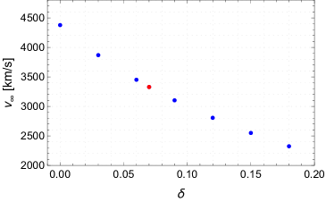
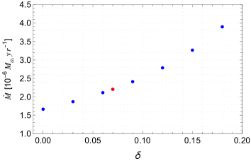
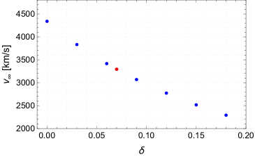
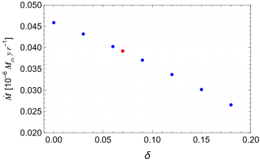
Figure 6: Dependence of the wind parameters as a function of the line-force parameter $\delta$. Upper panels are for $k=0.124$, and lower panels are for $k=0.0124$. The values obtained for our typical O5 V star without rotation are shown in red.

In the next subsections, we will discuss each of the slow solutions. The combined effect of the line-force parameters and the three physical wind solutions is discussed in detail in Venero et al. (2016).

Overall, the fast solution from the m-CAK theory has been very successful in explaining the terminal velocities and mass-loss rates of massive stars (see Lamers and Cassinelli, 1999; Kudritzki and Puls, 2000; Puls et al., 2008; Vink, 2022).

5.2 $\Omega$-slow solution

The original CAK model considered the star point approximation, i.e., all the photons are radially directed over the wind plasma. In that work, CAK only discussed the effect of the finite disk of the star seen by an observer in the wind. FA and PPK implemented the finite disk correction factor and solved the EoM. In both works, they also studied the influence of rotation in the equatorial plane of a rotating star, but they could not obtain solutions for rapidly rotating stars. The reason was found by Curé (2004), for $\Omega\gtrsim 0.75$, where $\Omega=v_{\rm{rot}}/v_{\rm{crit}}$. From this value of $\Omega$, the fast solution ceases to exist, and another type of solution is found. This solution called the $\Omega$-slow solution, is characterised by a slower and denser wind in comparison with the fast solution.

It is well known that Be stars are the fastest rotators among stars (Rivinius et al., 2013). Thus, in this section, we will study the topology and the wind solutions for a typical B2.5 V star with the following stellar and line force parameters: $T_{\rm eff}=20000K$, $\log g=4.11$, $R/R_{\odot}=4.0$, $k=0.61$, $\alpha=0.5$, and $\delta=0.0$. The lower (surface) boundary condition is fixed at $\rho_{*}=8.7\times 10^{-13}\,\mathrm{g/cm^{3}}$. In addition, the distortion of the shape of the star caused by its high rotational speed and gravity-darkening effects are not considered.

Fig. 7 shows the surfaces $R(u,Z)$, for different values of $\Omega$, together with the plane $R(u,Z)=0$. The intersection of the surfaces $R(u,Z)$ and $R(u,Z)=0$ (black lines) correspond to the locus of singular points. We clearly observe two different loci of singular points. The fast solution locus can be observed for $\Omega=0.3$ (upper left panel), $\Omega=0.5$ (upper right panel) and $\Omega=0.7$ (lower left panel). For larger rotational rates ($\Omega\gtrsim 0.75$), the fast solution locus lies completely under the plane $R(u,Z)=0$, as shown in the lower right panel for $\Omega=0.9$. Thus, the fast solution does not exist for large values of $\Omega$.

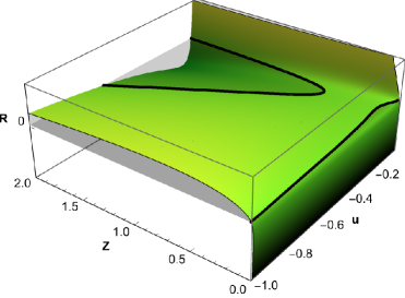
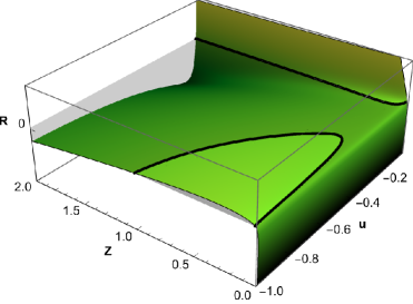
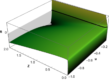
Figure 7: The function $R(u,Z)$ (topology) of the m-CAK theory as function of $\Omega$: $\Omega=0.3$ (upper left panel), $\Omega=0.5$ (upper right panel), $\Omega=0.7$ (lower left panel), and $\Omega=0.9$ (lower right panel). The plane $R(u,Z)=0$ is shown in light grey, and its intersection with the surface $R(u,Z)$ (locus of singular points) is plotted with black lines.

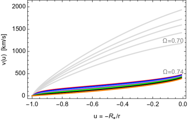
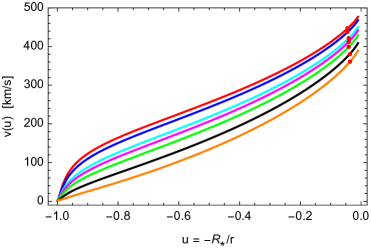
Figure 8: Velocity profiles, $v(u)$, as function of the rotational rate $\Omega$. Left panel: fast solutions ($\Omega\lesssim 0.74$) are plotted in grey lines, while the $\Omega$-slow solutions are in coloured lines: $\Omega=0.74$ (red line), $\Omega=0.76$ (blue line), $\Omega=0.80$ (cyan line), $\Omega=0.82$ (magenta line), $\Omega=0.85$ (green line), $\Omega=0.90$ (black line), and $\Omega=0.95$ (orange line). Right panel: The same $\Omega$-slow solutions, but zoomed and including the location of the singular points (red dots).

Figure 8 shows the velocity profiles, $v(u)$ as a function of $u$ for different values of $\Omega$. All these solutions use the same lower boundary condition. This figure shows (left panel) fast solutions in light grey and $\Omega$-slow solutions in coloured lines. The right panel shows only $\Omega$-slow solutions; the location of the singular point is almost independent of $\Omega$. This is a consequence of the shape of the locus curve of singular points (see Fig. 7). This locus is located almost at a constant value of $u$.

The $\Omega$-slow solutions are only valid in the equatorial plane in this 1D m-CAK model. Notice that this model does not take into account the oblateness and gravity-darkening effects. See Araya et al. (2017) for the implementation in the 1D model (equatorial plane) and Cranmer and Owocki (1995) for the implementation in the 2D model.
In the equatorial plane, the higher $\Omega$, the greater the centrifugal force and, consequently, the lesser the effective gravity. Therefore, the higher $\Omega$ is, the higher the rate of mass loss and, through the continuity equation, the higher the wind density, as shown in Fig.  9.

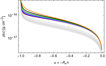
Figure 9: Wind density profiles, $\rho(u)$ (in gr/cm³) versus $u$, for fast and $\Omega$-slow solutions. The colour scheme is the same as the one used in Fig. 8

5.3 $\delta$-slow solution

The $\delta$-slow solution was found numerically by Curé et al. (2011). This solution, based on the m-CAK theory, describes the wind velocity profile when the ionization-related line-force parameter $\delta$ takes larger values, $\delta\gtrsim 0.28$. These values are larger than the ones provided by the standard m-CAK solution (see, Lamers and Cassinelli, 1999, and references therein). Nevertheless, Puls et al. (2000) calculated the value of $\delta$ for a pure Hydrogen atmosphere finding a value of $\delta\sim 1/3$. These high values of $\delta$ are also found in atmospheres and winds with extremely low metallicities (see, Kudritzki, 2002).

The $\delta$-slow solution, as well as the $\Omega$-slow solution, is characterized by low velocities. This solution could explain the velocities obtained for late-B and A-type supergiant stars and seems to fit well the observed anomalous correlation between the terminal and escape velocities found in A supergiant stars (Curé et al., 2011). Furthermore, in Venero et al. (2016, see their table 2), a gap of solutions, between the fast and the $\delta$-slow solutions, for different values of the rotational speed, was found in the plane $\delta$-$\Omega$.

To present the topological analysis of this type of solution, we adopt the model T19 from Venero et al. (2016). The stellar and line-force parameters are $T_{\rm eff}=19000K$, $\log g=2.5$, $R/R_{\odot}=40$, $k=0.32$, and $\alpha=0.5$. We use $\tau_{*}=2/3$ as a boundary condition at the stellar surface.

In Fig. 10, the $R(u,Z)$ function and the plane $R(u,Z)=0$ are shown for different values of $\delta$. The upper left panel shows the surface $R(u,Z)$ for $\delta=0.1$. We clearly see that for this case, the locus of singular points for fast solutions is different from the case of the fast solution shown in Fig. 1. Here this locus is located when $Z\lesssim 0.5$, $\forall\,u$. The upper right panel shows $R(u,Z)$ for $\delta=0.12$, where the locus of singular points for fast solutions returns to the behaviour shown in Fig. 1. The fast solution is present until $\delta=0.24$; see the lower left panel. We cannot find fast solutions for slightly larger values of $\delta$ until $\delta\sim 0.30$ (lower right panel). For this value of $\delta$, the locus of singular points for fast solutions shifts to slightly larger values of $Z$ for $u\lesssim-1$, and the numerical wind solutions no longer have a singular point in this locus, switching to the other locus of singular points ($\delta$-slow solutions) located at $u\lesssim-0.1$ (or $r\gtrsim 10R_{*}$).

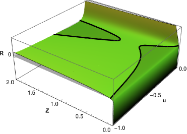
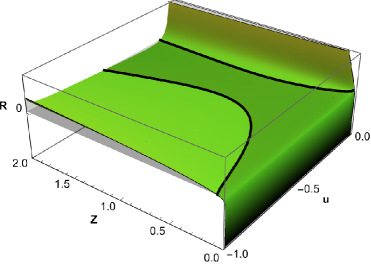
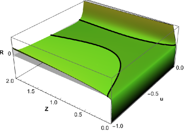
Figure 10: The topological function $R(u,Z)$ of the m-CAK theory as function of $\delta$. Upper left panel: $\delta=0.1$. Upper right panel: $\delta=0.12$. Lower left panel: $\delta=0.24$. Lower right panel: $\delta=0.3$. The plane $R(u,Z)=0$ is shown in light grey, and its intersection with the surface $R(u,Z)$ (locus of singular points) is plotted with black lines.

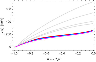
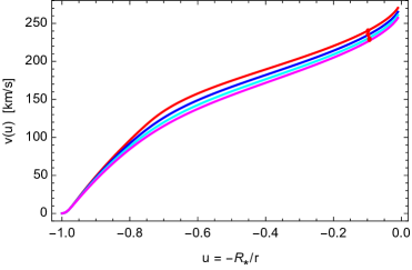
Figure 11: Velocity profiles, $v(u)$, for different values of the line-force parameter $\delta$. Left panel: fast solutions are plotted in grey lines for $\delta=0.0,0.1,0.2,0.24$, while $\delta$-slow solutions are in coloured lines. Red line corresponds to $\delta=0.3$, blue line to $\delta=0.31$, cyan line to $\delta=0.32$, and magenta line to $\delta=0.33$. The right panel shows only $\delta$-slow solutions, and the location of the singular points for each solution is shown with a red dot.

5.4 The $\beta$-law approximation

In the work of PPK, after obtaining the numerical solution of the EoM, they assumed a power law approximation to describe the velocity profile only as a function of the radial coordinate $r$. This approximation is known as the $\beta$-law approximation and has the following expression:

$$v(r) = v_{\infty}\,(1-R_{\ast}/r)^{\beta}\,,$$ (62)

$$= v_{\infty}\,(1+u)^{\beta}\,,$$ (63)

where $v_{\infty}$ is the terminal velocity and the value of $\beta$ determine the shape of the velocity profile. In the context of stellar wind diagnostics, these parameters are considered fit parameters that must be determined through spectral line fitting. Usually, the range used for the $\beta$ parameter is $0.7\lesssim\beta\lesssim 4$ (Kudritzki and Puls, 2000).

Figure 12 shows the velocity profile of the fast solution for the stellar and line-force parameters given at the beginning of section 5.1, together with six different values of $\beta$ for a $\beta$-law velocity profile. From this figure, we can conclude that the fast solution cannot be described properly by a $\beta$-law with $\beta>1.2$.

On the other hand, Figure 13 shows the velocity profile for the $\delta$-slow solution for the stellar and line-force parameters given at the beginning of section 5.3, and $\delta=0.32$. Also, the same $\beta$-law profiles of Fig. 12 are used, with the proper values of $v_{\infty}$ for this solution. The same is plotted in Fig. 14 for the $\Omega$-slow solution with a $\Omega=0.8$. In the case of the $\delta$-slow solution, the $\beta$-law profile cannot fit the m-CAK hydrodynamical solution for any $\beta>0.7$, while for values around to $\beta=0.7$ the profiles can be considered similar. Finally, from Fig. 14, we can definitely conclude that $\Omega$-slow solutions cannot be described properly by any $\beta$-law profile.

Figure 12: Fast solution velocity profile (solid blue), $v(u)$ vs. $u$. Six different $\beta$-law velocity profiles are also plotted. It is clearly seen that the $\beta$-law approximation is a good one for $0.7\lesssim\beta\lesssim 1.2$. See text for details.

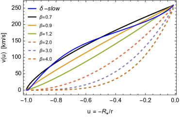
Figure 13: $\delta$-slow solution velocity profile (solid blue), $v(u)$ vs. $u$. Six different $\beta$-law velocity profiles are also plotted. For values around to $\beta=0.7$ the profiles can be considered similar, but it can be clearly concluded that for $\beta>0.7$, the $\beta$-law profile cannot fit the m-CAK hydrodynamical $\delta$-slow solution.

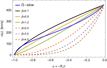
Figure 14: $\Omega$-slow solution velocity profile (solid blue), $v(u)$ vs. $u$. Six different $\beta$-law velocity profiles are also plotted. It can be clearly concluded that no $\beta$-law profile can fit the m-CAK hydrodynamical $\Omega$-slow solution.

6 Analytical wind solutions

Using an analytical expression to represent the radiation force and solve the equation of motion analytically offers numerous advantages over the numerical integration of the EoM. These formulae can be used in all cases where good first estimates are needed; for example, it gives the advantage of solving the radiative transfer problem for moving media in an easier way.

KPPA were one of the first to develop analytical solutions for radiation-driven winds considering the finite disk correction factor in the line force. Based on these solutions, they provided approximated analytical expressions for the terminal velocity and the mass loss rate in terms of the stellar parameters ($L$, $M_{\ast}$ and $R_{\ast}$), the line force parameters ($k$, $\alpha$ and $\delta$) and the free parameter $\beta$ from the $\beta$-law (they adopted $\beta=1.0$ for their results).

Other authors have tried to simplify the complicated numerical treatment from the theory. Villata (1992) (hereafter V92), with the purpose of simplifying the integration of the EoM, derived an approximated expression for the line acceleration term, which depends only on the radial coordinate. Müller and Vink (2008) (hereafter MV08) presented an analytical expression for the velocity field using a parameterized description for the line acceleration that (as in V92’s) also depends on the radial coordinate. These line-acceleration expressions do not depend on the velocity or the velocity gradient, as the standard m-CAK description does. Araya et al. (2014) proposed to achieve a complete analytical description of the 1-D hydrodynamical solution for radiation-driven winds in the fast regime by gathering the advantages of both previous approximations (the use of known parameters and the Lambert$W$ function). In addition, Araya et al. (2021) developed an analytical solution for the $\delta$-slow regime. To date, no approximation using the Lambert$W$ function has been performed for the $\Omega$-slow regime, we expect to do this in the future.

In the next sections, we describe the results and methodology used to solve analytically the equation of motion for fast and $\delta$-slow regimes.

6.1 Solution of the dimensionless equation of motion

In this section, we recapitulated the methodology described by MV08 to obtain the dimensionless equation of motion.

In a dimensionless form, the momentum equation can be expressed as follows,

$$\hat{v}\,\frac{d\hat{v}}{d\hat{r}}=-\frac{\hat{v}_{\rm{crit}}^{2}}{\hat{r}^{2}}+\hat{g}^{\rm{line}}-\frac{1}{\rho}\frac{d\rho}{d\hat{r}},$$ (64)

where $\hat{r}$ is a dimensionless radial coordinate $\hat{r}=r/R_{*}$, and the dimensionless velocities (in units of the isothermal sound speed $a$) are:

$$\hat{v}=\frac{v}{a}\>\>\>\>\>\mathrm{and}\>\>\>\>\>\hat{v}_{\rm{crit}}=\frac{v_{\rm{esc}}}{a\sqrt{2}},,$$ (65)

here, $v_{\rm{crit}}$ is the rotational break-up velocity in the case of a rotating star. It is usually determined by dividing the effective escape velocity, $v_{\rm{esc}}$, by a factor of $\sqrt{2}$. Similarly, a dimensionless line acceleration can be written as follows:

$$\hat{g}^{\rm{line}}=\frac{R_{*}}{a^{2}}\,g^{\rm{line}}.$$ (66)

Using the continuity equation and the equation of state of an ideal gas, the dimensionless equation of motion reads as follows:

$$\left(\hat{v}-\frac{1}{\hat{v}}\right)\frac{d\hat{v}}{d\hat{r}}=-\frac{\hat{v}_{\rm{crit}}^{2}}{\hat{r}^{2}}+\frac{2}{\hat{r}}+\hat{g}^{\rm{line}}(\hat{r}).$$ (67)

Lastly, a 1-D velocity profile is derived analytically in terms of Lambert$W$ function (Corless et al., 1993, 1996; Cranmer, 2004). See MV08 for a detailed description of the methodology used to arrive at this solution. This analytical solution is expressed as follows:

$$\hat{v}(\hat{r})=\sqrt{-W_{j}(x(\hat{r}))},$$ (68)

where

$$x(\hat{r})=-\left(\frac{\hat{r}_{\rm c}}{\hat{r}}\right)^{4}\,\exp\left[-2\,\hat{v}^{2}_{\rm{crit}}\left(\frac{1}{\hat{r}}-\frac{1}{\hat{r}_{\rm c}}\right)-2\int_{\hat{r}_{\rm c}}^{\hat{r}}\hat{g}^{\rm{line}}(\hat{r})d\hat{r}-1\right]\,.$$ (69)

In the last equation appears the parameter $\hat{r}_{\rm c}$, which represents the position of the sonic (or critical) point.

Also, the Lambert$W$ function ($W_{j}$) has only two real branches, indicated by the sub-index j, where $j=0,-1$. These two branches coincide at the sonic point, $\hat{r_{\rm c}}$, i.e.,

$$j=\left\{\begin{array}[]{r r c}0&\mathrm{for}&1\leq\hat{r}\leq\hat{r}_{\rm c}\\ -1&\mathrm{for}&\hat{r}>\hat{r}_{\rm c},\end{array}\right.$$ (70)

A regularity condition must be imposed, as in the m-CAK case, since the LHS of the equation of motion (Eq. 67) vanishes at $\hat{v}=1$ (singularity condition in CAK formalism). This is equivalent to ensuring that the RHS of Eq. (67) vanishes at $\hat{r}=\hat{r}_{\rm c}$. Therefore,

$$-\frac{\hat{v}_{\rm{crit}}^{2}}{\hat{r}_{c}^{2}}+\frac{2}{\hat{r}_{c}}+\hat{g}^{\rm{line}}(\hat{r}_{c})=0,$$ (71)

and $\hat{r}_{\rm c}$ is obtained by solving this last equation. Finally, the velocity profile is derived using the function $x(\hat{r})$, Eq. (69), into Eq. (68).

6.2 The fast regime

KPPA’s analytical study of radiation-driven stellar winds allowed V92 to derive an approximate expression for the line acceleration term. In this case, the line acceleration is only dependent on the radial coordinate, and it reads as follows:

$$g^{\mathrm{line}}_{\mathrm{V92}}(\hat{r})=\frac{G\,M_{*}\,(1-\Gamma_{e})}{R_{*}^{2}\,\hat{r}^{2}}\,A(\alpha,\beta,\delta)\left(1-\frac{1}{\hat{r}}\right)^{\alpha(2.2\,\beta-1)}\,,$$ (72)

with

$$A(\alpha,\beta,\delta)=\frac{(1.76\,\beta)^{\alpha}}{1-\alpha}\left[10^{-\delta}(1+\alpha)\right]^{1/(1-\alpha)}\left[1+\left(\frac{2}{\alpha}\left\{1-\left[10^{-\delta}(1+\alpha)\right]^{1/(\alpha-1)}\right\}\right)^{1/2}\right]^{\alpha}.$$ (73)

According to Kudritzki et al. (1987), the exponent $\beta$ can be calculated based on the force multiplier parameters and the escape velocity, $v_{\rm{esc}}$:

$$\beta=0.95\,\alpha+\frac{0.008}{\delta}+\frac{0.032\,v_{\rm{esc}}}{500},$$ (74)

with $v_{\rm{esc}}$ in km/s.

Then, using Eq. (72) in its dimensionless form (Eq. 66) and inserting it into the dimensionless equation of motion (Eq. 67), it yields:

$$\left(\hat{v}-\frac{1}{\hat{v}}\right)\frac{d\hat{v}}{d\hat{r}}=-\frac{\hat{v}_{\rm{crit}}^{2}}{\hat{r}^{2}}+\frac{2}{\hat{r}}+\frac{1}{a^{2}}\frac{GM_{*}(1-\Gamma_{e})}{R_{*}\,\hat{r}^{2}}\,A(\alpha,\beta,\delta)\left(1-\frac{1}{\hat{r}}\right)^{\gamma_{\rm v}},$$ (75)

with $\gamma_{\rm v}\,=\,{\alpha\,(2.2\,\beta-1)}.$

Based on V92’s approximation of the line acceleration, this differential equation can be viewed as a solar-like differential equation of motion. Hence, the singular point is the sonic point. Additionally, V92’s equation of motion does not have eigenvalues, which means it doesn’t depend explicitly on the star’s mass loss rate.

Using a standard numerical integration method, V92 solved the equation of motion and obtained terminal velocities that were within 3-4 $\%$ of those computed by PPK and KPP.

A parametrized description of line acceleration was presented years later by MV08 that is dependent on the radial coordinate (like V92’s). The line acceleration in MV08 was determined using Monte-Carlo multi-line radiative transfer calculations (de Koter et al., 1997; Vink et al., 1999) and a $\beta$ law. Following this, the line acceleration was fitted using the following formula:

$$\hat{g}^{\mathrm{line}}_{\mathrm{MV08}}(\hat{r})=\frac{\hat{g}_{0}}{\hat{r}^{1+\delta_{1}}}\left(1-\frac{\hat{r_{0}}}{\hat{r}^{\delta_{1}}}\right)^{\gamma},$$ (76)

where $\hat{g_{0}}$, $\delta_{1}$, $\hat{r_{0}}$ and $\gamma$ are the acceleration line parameters.

Then, the solution of the equation of motion, based on their methodology and line acceleration, is:

$$\hat{v}(\hat{r})=\sqrt{-W_{j}(x(\hat{r}))}\,,$$ (77)

with

$$x(\hat{r})= -\left(\frac{\hat{r}_{\rm c}}{\hat{r}}\right)^{4}\exp\left[-2\,\hat{v}^{2}_{\rm{crit}}\left(\frac{1}{\hat{r}}-\frac{1}{\hat{r}_{\rm c}}\right)\right.$$

$$-\frac{2}{\hat{r}_{0}}\frac{\hat{g}_{0}}{\delta_{1}\,(1+\gamma)}\left(\left.\left(1-\frac{\hat{r}_{0}}{\hat{r}^{\delta_{1}}}\right)^{1+\gamma}-\left(1-\frac{\hat{r}_{0}}{\hat{r}_{\rm c}^{\delta_{1}}}\right)^{1+\gamma}\right)-1\right].$$ (78)

As a result of the approximations described above, the velocity profile can be represented analytically, greatly simplifying the solution of the equation of motion.

Also, it is relevant to note that each of the mentioned approximations has its own advantages and disadvantages. Even though Villata’s approximation of the radiation force is general and can directly be applied to describe any massive star’s wind, the momentum equation still needs to be solved numerically. With MV08’s approximation, the equation of motion can be analytically solved, based on $\hat{g}_{0}$, $\delta_{1}$, $\hat{r}_{0}$, and $\gamma$ parameters of the star. Nevertheless, it is still necessary to perform Monte Carlo multi-line radiative transfer calculations in order to determine these parameters.

This methodology to solve the equation of motion was revisited by Araya et al. (2014), and in order to derive a fully analytical expression combining V92’s expression of the equation of motion, with the methodology developed by MV08.
This analytical solution is,

$$\hat{v}(\hat{r})=\sqrt{-W_{j}(x(\hat{r}))},$$ (79)

with

$$x(\hat{r})=-\left(\frac{\hat{r}_{\rm c}}{\hat{r}}\right)^{4}\,\exp\left[-2\,\hat{v}^{2}_{\rm{crit}}\left(\frac{1}{\hat{r}}-\frac{1}{\hat{r}_{\rm c}}\right)-2\left(I_{\hat{g}_{V92}^{\rm{line}}}(\hat{r})-I_{\hat{g}_{V92}^{\rm{line}}}(\hat{r}_{\rm c})\right)-1\right]\,,$$ (80)

where

$$I_{\hat{g}_{V92}^{\rm{line}}}(\hat{r})= \left(10^{-\delta}\,(1+\alpha)\right)^{\frac{1}{1-\alpha}}\,\left(1+\sqrt{2}\sqrt{-\frac{\left(10^{-\delta}\,(1+\alpha)-1\right)^{\frac{1}{\alpha-1}}}{\alpha}}\right)^{\alpha}$$

$$\times(1.76\,\beta)^{\alpha}\,G\,M_{*}\left(\frac{\hat{r}-1}{\hat{r}}\right)^{1+\gamma_{\rm v}}\frac{\Gamma-1}{\left(a^{2}[\alpha-1](1+\gamma_{\rm v})\,R_{*}\right)}.$$ (81)

As was mentioned in the previous section, $\hat{r}_{\rm c}$ can be obtained numerically, making the RHS of Eq. (75) equal zero. In order to obtain the terminal velocity in a simpler way, we can use the average value of $\hat{r}_{c}$ ($\overline{\hat{r}}_{c}=1.0026$) obtained by Araya et al. (2014). Note that this value can be used only in the supersonic region.

Equation (79) has the advantage that it is based not only on the Lambert$W$ function but also on stellar parameters and the line force parameters. For a wide range of spectral types, stellar and force multiplier parameters are given (see, e.g., Abbott, 1982; Pauldrach et al., 1986; Lamers and Cassinelli, 1999; Noebauer and Sim, 2015; Gormaz-Matamala et al., 2019; Lattimer and Cranmer, 2021).

By comparing the analytical solution to the 1-D hydrodynamic code Hydwind, the accuracy of the analytical solution can be tested. Figure 15 compares the results obtained with our analytical approximation to those obtained with the hydrodynamics for four stars taken from Araya et al. (2014). Both solutions have similar behaviours. However, as shown by Araya et al. (2014), the analytical approximation close to the stellar surface (subsonic region) is not good enough. In the same way, Figure 16 compares the numerical and analytical velocity profiles near to the stellar surface for $\epsilon$ Ori.

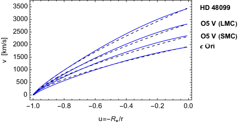
Figure 15: Velocity profiles as function of the inverse radial coordinate $u=-R_{*}/r=-1/\hat{r}$ for four models. The hydrodynamic results from Hydwind are shown in solid blue lines, and the analytical solutions are in dashed lines. The stellar and line-force parameters for the models are given in Araya et al. (2014).

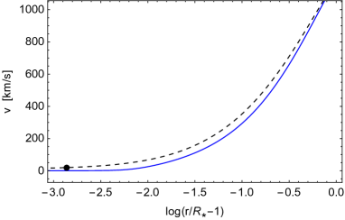
Figure 16: Velocity profiles of $\epsilon$ Ori as a function of $\log(r/R_{\ast}-1)$ in a region near to the stellar surface. The solid blue line shows the numerical hydrodynamic result, and the analytical solution is in dashed line. The dot symbol indicates the position of the sonic (or critical) point. The difference between both curves is around one thermal speed.

There is a limitation to this analytical expression when the line force parameter $\delta$ exceeds about $0.3$. This is due to the complexity of a term in the proposed line acceleration expression. To obtain an expression with real values, high values of $\delta$ would require high values of $\alpha$. However, such kind of $\alpha$ values would be totally unphysical ($\alpha>1$). As an illustration of the dependence of this expression on the parameters $\alpha$ and $\delta$, Fig. 17 shows the domain of the complex and real regions when this expression is evaluated to the given line acceleration term.

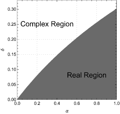
Figure 17: Real and complex regions where the line acceleration expression given by Villata (1992) can be found. These regions are delimited by the values of the line-force parameters $\alpha$ and $\delta$.

6.3 The $\delta$-slow regime

Considering the results obtained when using an approximate description of the wind velocity for the $\delta$-slow case, Araya et al. (2021) modified the function of the line acceleration given by MV08 to better describe of the $\delta$-slow wind.

As a result, the proposed line acceleration is:

$$\hat{g}^{\rm{line}}(\hat{r})=\frac{\hat{g}_{0}}{\hat{r}^{1+\delta_{1}}}\left(1-\frac{1}{\hat{r}^{\delta_{2}}}\right)^{\gamma},$$ (82)

where $\hat{g}_{0}$, $\delta_{1}$, $\delta_{2}$, and $\gamma$ are the new set of line acceleration parameters.

It is notable that the $\delta_{2}$ parameter, which has been incorporated into this new expression, provides a much better agreement with the numerical line acceleration obtained from the m-CAK model in the $\delta$-slow regime compared with the one from MV08.

Based on this new definition of the radiation force, the new dimensionless equation of motion reads:

$$\left(\hat{v}-\frac{1}{\hat{v}}\right)\frac{d\hat{v}}{d\hat{r}}=-\frac{\hat{v}_{{\rm crit}}^{2}}{\hat{r}^{2}}+\frac{2}{\hat{r}}+\frac{\hat{g}_{0}}{\hat{r}^{1+\delta_{1}}}\left(1-\frac{1}{\hat{r}^{\delta_{2}}}\right)^{\gamma}.$$ (83)

The Lambert$W$ function is used to solve the equation of motion, Eq. (83) following the same methodology developed by MV08,

$$\hat{v}(\hat{r})=\sqrt{-W_{j}(x(\hat{r}))}\,,$$ (84)

with

$$x(\hat{r})=-\left(\frac{\hat{r}_{\rm c}}{\hat{r}}\right)^{4}\,\exp\left[-2\,\hat{v}^{2}_{\rm{crit}}\left(\frac{1}{\hat{r}}-\frac{1}{\hat{r}_{\rm c}}\right)-2\left(I_{\hat{g}^{\rm{line}}}(\hat{r})-I_{\hat{g}^{\rm{line}}}(\hat{r}_{\rm c})\right)-1\right],$$

where

$$I_{\hat{g}^{\rm{line}}}=\int\hat{g}^{\rm{line}}(\hat{r})d\hat{r}=-\frac{g_{0}\,\hat{r}^{-\delta_{1}}\,{{}_{2}F_{1}}\left[-\gamma,\frac{\delta_{1}}{\delta_{2}},1+\frac{\delta_{1}}{\delta_{2}},\hat{r}^{-\delta_{2}}\right]}{\delta_{1}},$$ (85)

being ${{}_{2}F_{1}}$ the Gauss Hypergeometric function. The critical (or sonic) point, $\hat{r}_{\rm c}$, is obtained numerically, making the RHS of Eq. (83) equal zero.

Ultimately, this expression for the velocity profile is in quite satisfactory agreement with the numerical solution from Hydwind.

As described in Araya et al. (2014), a relationship was established between the MV08 line-force parameters ($\hat{g_{0}}$, $\delta_{1}$, $\hat{r_{0}}$, and $\gamma$) and the stellar and m-CAK line-force parameters. In addition to being easy to use, this relationship provides a straightforward and versatile method of calculating velocity profiles analytically for a wide range of spectral types since both stellar and m-CAK line force parameters are available (see, Abbott, 1982; Pauldrach et al., 1986; Lamers and Cassinelli, 1999; Noebauer and Sim, 2015; Gormaz-Matamala et al., 2019; Lattimer and Cranmer, 2021).

A similar relationship can be derived for the $\delta$-slow regime using m-CAK hydrodynamic models, that is, creating a grid of Hydwind models for $\delta$-slow solutions. These models are then analysed using a multivariate multiple regression analysis (MMR Rencher and Christensen, 2012; Mardia et al., 1980).

To develop this hydrodynamic grid, the stellar radius is calculated from $M_{\rm{bol}}$ for each pair of stellar parameters ($T_{\rm{eff}}$, $\log\,g$) by using the flux weighted gravity-luminosity relationship (Kudritzki et al., 2003, 2008). Additionally, a total of 20 stellar radius values were added (ranging from 5 $R_{\odot}$ to 100 $R_{\odot}$ in steps of 5 $R_{\odot}$). Surface gravities are in the range of $\log g=2.7$ down to about $90\%$ of Eddington’s limit in steps of 0.15 dex. Effective temperatures are between $9\,000$ K to $19\,500$ K, in steps of 500 K. The range of this grid has been chosen to cover the region of the $T_{\rm{eff}}$-$\log\,g$ diagram that contains B- and A-type supergiants. In Table 1, the m-CAK line-force parameters for each set of $(T_{\rm{eff}}$, $\log\,g$) values are listed. For the purpose of obtaining $\delta$-slow solutions, only high values of $\delta$ are considered. For the $T_{\rm{eff}}$-$\log\,g$ plane (see Fig. 18), we show in blue dots all converged models.

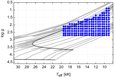
Figure 18: Hydrodynamic models in the $T_{\rm{eff}}$-$\log\,g$ plane. Blue dots represent the converged solutions. Grey solid lines are the evolutionary tracks for stars of $7M_{\odot}$ to $60M_{\odot}$ without rotation (Ekström et al., 2012), and black lines represent the zero-age main sequence (ZAMS) and the terminal age main-sequence (TAMS).

Table 1: m-CAK line-force parameter ranges for the grid of models.

Parameter	Range
$\alpha$	0.45 - 0.69 (step size of 0.02)
$k$	0.05 - 1.00 (step size of 0.05)
$\delta$	0.26 - 0.35 (step size of 0.01)

In order to obtain the new line acceleration parameters ($\hat{g}_{0}$, $\delta_{1}$, $\delta_{2}$, and $\gamma$) for each model, the m-CAK line acceleration was fitted, using Least Squares, with the proposed line acceleration expression (Eq. 82). Then, a MMR is applied to the grid of models in order to derive the relationship between new line acceleration parameters ($\hat{g}_{0}$, $\delta_{1}$, $\delta_{2}$ and $\gamma$) and stellar ($T_{\mathrm{eff}}$, $\log\mathrm{g}$, $R_{*}/R_{\odot}$) and m-CAK line-force parameters ($k$, $\alpha$, $\delta$). The estimated parameters are:

$$\hat{g}_{0}^{0.27} = -4.548-1.890\times 10^{-4}\,T_{\mathrm{eff}}+$$

$$4.393\,\log\mathrm{g}+3.026\times 10^{-2}R_{*}/R_{\odot}-$$

$$4.802\times 10^{-3}\,k+3.781\,\alpha-3.212\,\delta,$$

$$(\delta_{1}+1)^{5.3} = -4.623-3.743\times 10^{-4}\,T_{\mathrm{eff}}+$$

$$1.489\times 10^{1}\,\log\mathrm{g}+1.148\times 10^{-1}R_{*}/R_{\odot}+$$

$$2.415\,k+9.553\times 10^{1}\,\alpha-1.320\times 10^{2}\,\delta,$$

$$\delta_{2}^{0.45} = 5.359+8.262\times 10^{-5}\,T_{\mathrm{eff}}-$$

$$1.327\,\log\mathrm{g}-8.327\times 10^{-3}R_{*}/R_{\odot}+$$

$$2.181\times 10^{-1}\,k+9.618\times 10^{-1}\,\alpha-2.296\,\delta$$

and

$$(\gamma+1)^{-3.56} = -1.031+7.254\times 10^{-6}\,T_{\mathrm{eff}}+$$

$$2.994\times 10^{-1}\,\log\mathrm{g}+3.097\times 10^{-3}R_{*}/R_{\odot}+$$

$$1.836\times 10^{-1}\,k-4.828\times 10^{-1}\,\alpha+1.254\,\delta,$$

After the estimated values for each dependent variable, $\hat{g}_{0}^{0.27}$, $(\delta_{1}+1)^{5.3}$, $\delta_{2}^{0.45}$, $(\gamma+1)^{-3.56}$, are obtained they are transformed into $\hat{g}_{0}$, $\delta_{1}$, $\delta_{2}$, and $\gamma$ through their respective inverse functions. Finally, we can use these parameters in Eq. (84) to calculate the velocity profile.

The velocity profiles obtained via Hydwind code and the analytical solution are shown in Fig. 19 for one model with $\delta$-slow solution. The model is taken from Curé et al. (2011).

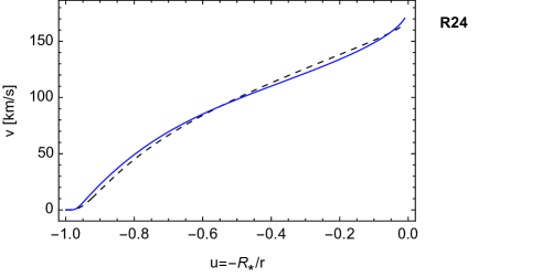
Figure 19: Velocity profiles as function of the inverse radial coordinate $u=-R_{*}/r=-1/\hat{r}$ for the model R24 from Curé et al. (2011). The hydrodynamic result from Hydwind is shown in the solid blue line, and the analytical solution is a dashed black line.

Remember, however, that this relationship holds only for $\delta$-slow solutions, especially for values of $\delta$ between $0.29$ and $0.35$. In addition, considering the number of converged models in the grid, the authors recommend using this expression for values of $\alpha$ between $0.45$ and $0.55$.

Finally, it is important to remark that both analytical solutions for the velocity profile, fast and $\delta$-slow, do depend only on the stellar ($T_{\mathrm{eff}}$, $\log\mathrm{g}$, $R_{*}/R_{\odot}$) and m-CAK line-force parameters ($k$, $\alpha$, $\delta$). Regarding to the mass-loss rate, V92 proposed an expression to obtain it (in terms of the stellar and m-CAK parameters) following the approximations given by Kudritzki et al. (1989). Also, Araya et al. (2021), in the appendix, proposed a method to obtain the mass-loss based on Curé (2004).

7 Summary and discussion

Observations over the past decades have shown that the basic wind parameters behave as predicted by the theory. This fundamental agreement between observations and theory provides strong evidence that the winds from massive stars are driven by radiation pressure. This has given the m-CAK theory a well-established status in the massive star community. However, several issues are contentious and still unclear, such as the calibration of the Wind-momentum Luminosity Relationship (WLR) (Kudritzki et al., 1995), disks of Be stars, wind parameters determination, the applicability of the called slow wind solutions, among others. All these issues are the focus of massive stars research.

This review is focused on the theoretical and numerical research of wind hydrodynamics of massive stars based on the m-CAK theory, with particular emphasis on its topology and hydrodynamic solutions.

We presented a topological analysis of the one-dimensional m-CAK hydrodynamic model and its three known hydrodynamic solutions, the fast, $\Omega$-slow and $\delta$-slow solutions. From a topological point of view, slow solutions are obtained from a new branch of solutions with a locus of singular points far from the stellar surface, unlike fast solutions with a family of singular points near the stellar surface.

We continued analyzing the dependence of the line force parameters ($k$, $\alpha$, and $\delta$) with the wind parameters (mass loss rate and terminal velocity) in order to understand the complex non-linear dependence between these parameters. In the case of $\alpha$, there is an increase in both wind parameters as this parameter increases. This behaviour is similar to the $k$ parameter, but the dependence is very slight for terminal velocity, while the mass loss rate has a significant impact. For the $\delta$ parameter, the terminal velocity has a decreasing behaviour when this parameter increases, while the mass-loss rate can have a decreasing or increasing behaviour, which depends on the parameter $k$. When $k$ is low, mass-loss rates decrease, while $\delta$ increases, whereas when $k$ is large, the opposite occurs.

In addition, we compared the $\beta$-law with the hydrodynamic solutions. We concluded that the fast solution could not be adequately described by a $\beta$-law with $\beta>1.2$, while the $\delta$-slow solution cannot be described by any $\beta$-law.

Furthermore, we presented two analytical expressions for the solution of line-driven winds in terms of the stellar and line-force parameters. The expressions are addressed to obtain the fast and $\delta$-slow velocity regimes in a simple way. Both solutions are based on the Lambert$W$ function and an approximative expression for the wind line acceleration as a function of the radial distance. The importance of an analytical solution lies in its simplicity in studying the properties of the wind instead of solving complex hydrodynamic equations. In addition, these analytical expressions can be used in radiative transfer or stellar evolution codes (see, e.g., Gormaz-Matamala et al., 2022).

Concerning the applicability of the slows solutions, in the case of the $\Omega$-slow solution, their behaviour suggest that it can play a paramount role in the ejection of material to the equatorial circumstellar environment of Be and B[e] stars. Be stars are a unique set of massive stars whose main distinguishing characteristics are rapid rotation and the presence of a dense, gaseous circumstellar disk orbiting in a quasi-Keplerian fashion. There is a long-standing problem in understanding the formation of disks in Be stars; this is one of the major areas of ongoing research in Be stars. The gaseous disks are not remnants of the objects’ protostellar environments, nor are they formed through the accretion of material Porter and Rivinius (2003); Rivinius et al. (2013). On the contrary, the equatorial gas consists of a decretion disk formed from a material originating from the central star.

As was stated above, attempts to solve this problem have been made without much success, for example, the link between the line-driven winds and these discs, called the Wind Compressed Disk (Bjorkman and Cassinelli, 1993), but the work of Owocki et al. (1996) was the first to show this is not a viable mechanism for rapidly rotating stars due to the non-radial line force components. The most accepted model to successfully reproduce many Be star observables is the viscous decretion disk (VDD) model, developed by Lee et al. (1991) and examined by Okazaki (2001), Bjorkman and Carciofi (2005), Krtička et al. (2011) and Curé et al. (2022). Currently, how that material is ejected into the equatorial plane and how sufficient angular momentum is transferred to the disk to maintain quasi-Keplerian rotation are among the primary unresolved questions currently driving classical Be star research.

Araya et al. (2017) studied the $\Omega$-slow wind solution and its relation with the disks of Be stars. Overall, this work is an extension to the study done by Silaj et al. (2014), where they precisely investigated if the density distribution provided by the $\Omega$-slow wind solution could adequately describe the physical conditions to form a dense disc in Keplerian rotation via angular momentum transfer. They considered a two-component wind model, i.e., a fast, thin wind in the polar latitudes and a $\Omega$-slow, dense wind in the equatorial regions. Based on the equatorial density distributions, H$\alpha$ line profiles are generated and compared with an ad-hoc emission profile, which agrees with the observations. In addition, their calculations assumed three different scenarios related to the shape (oblate correction factor) and the star’s brightness (gravity darkening). Finally, they found that under certain conditions (related to the line-force parameter of the wind), a significant H$\alpha$ line profile could be produced, and maybe the line-driven winds through the $\Omega$-slow solution can have an essential role in the disc formation of Be stars.

In addition, Araya et al. (2018) studied the zone where the classical m-CAK fast solution ceases to exist, and the $\Omega$-slow solution emerges at rapid rotational speeds. This study used two hydrodynamic codes with time-dependent and stationary approaches. They found that both solutions can co-exist in this transition region, which depends exclusively on the initial conditions. In addition, they performed base-density wind perturbations to test the stability of the solution within the co-existence region. A switch of the solution was found under certain perturbation conditions. The results are addressed to a possible role in the ejection of extra material into the equatorial plane via pulsation modes, where the $\Omega$-slow solution can play an important role.

A current weakness of this m-CAK model is that it does not consider the role of viscosity and its influence on angular momentum transport. This mechanism might explain the formation of a Keplerian disc.

On the other hand, the $\delta$-slow solution is promising to explain the discrepancies of the wind parameters between observations and theory in late B- and A-type supergiant stars. According to the findings of Venero et al. (2016), these suggest that the terminal velocity of early and mid-B supergiants agrees with the results seen from fast outflowing winds. By contrast, the results obtained for late B supergiants and, mainly, those obtained for early A supergiants agree with the results achieved for $\delta$-slow stationary outflowing wind regimes. Then, the $\delta$-slow solution enables us to describe the global features of the wind quite well, such as mass-loss rates and terminal velocities of moderately and slowly rotating B supergiants.

Conversely, Venero et al. (2016) stated that the $\delta$-slow solution seems not to be present in stars with $T_{\rm{eff}}>21\,000$ K. This restricts the possibility of a switch between fast and slow regimes at such temperatures. Consequently, this would be a physical explanation for why an empirical bi-stability jump can be observed around $21\,000$ K in B supergiants (Lamers et al., 1995). From a theoretical perspective, a velocity jump has also been found using Monte Carlo modelling and the co-moving frame method (see, e.g., Vink, 2018; Vink and Sander, 2021; Vink, 2022)

In addition, it is generally accepted that most O and early B-type stars can be adequately modelled with a $\beta$ velocity law with $0.7\lesssim\beta\lesssim 1.2$. However, supergiants A and B exhibit $\beta$ values that tend towards higher values, often $\beta\geq 2$ (see, e.g., Stahl et al., 1991; Lefever et al., 2007; Markova and Puls, 2008; Haucke et al., 2018; Rivet et al., 2020). Venero et al. 2023 (in preparation) propose that $\delta$-slow solutions might explain these winds. They show that the $\delta$-slow regime could adequately fit the H$\alpha$ line profile of B supergiants with the same accuracy as that obtained using a $\beta$-law with $\beta\geq 2$, but now with a hydrodynamic explanation of the velocity profile used.

The investigation carried out in the latest works inspired us to go deeper into the possible role of slow wind solutions with respect to the unresolved questions related to massive stars. In view of our results, we are encouraged to develop this line of research further. In the case of the $\Omega$-slow solution and its link to Be stars, or possibly to B[e] stars, it would require 2D/3D models for a better understanding to take into account non-radial forces, the effects of stellar distortion and gravity darkening. These considerations could change, in turn, the nature of the $\Omega$-slow solution or the behaviour regarding the co-existence of solutions and a switch between them.
The $\delta$-slow solution could play an essential role in understanding the winds of B- and A-type supergiants. Moreover, this solution is expected to solve the disagreement between the observations and theory for these stars and, in this way, calibrate the wind-momentum luminosity relationship.

As we mentioned previously. In the standard procedure for finding stellar and wind parameters, the $\beta$-law ($\beta$, $v_{\infty})$ and a mass-loss rate ($\dot{M}$) are three ’free’ input parameters in radiative transfer codes, comparing synthetic spectra with the observed spectra of a star. The $\beta$ law comes from an approximation of the fast wind solutions, and the values of $\beta$ should be in a restricted interval. To improve the hydrodynamic approximation used in this standard procedure, we have developed two hydrodynamic procedures to derive stellar and wind parameters:

• The self-consistent CAK procedure (Gormaz-Matamala et al., 2019), based on the m-CAK model. Here we iteratively calculate the line-force parameters using the atomic line database from CMFGEN, coupled with the m-CAK hydrodynamic until convergence. We obtain the line-force parameters and, therefore, the velocity profile and the mass-loss rate. Thus, none of the input parameters are ’free’, but self-consistently calculated.

• The Lambert$W$ procedure (Gormaz-Matamala et al., 2021). In this procedure, we start using a $\beta$-law and a value for $\dot{M}$ in CMFGEN. After convergence, we calculated the line acceleration as a function of $r$, and using the Lambert$W$ function we obtain a new velocity profile. This is inserted in CMFGEN and the cycle is repeated until convergence. In this Lambert$W$ procedure, the only input parameter is the mass-loss rate.

We expect that these two alternatives, which reduce the number of input parameters, will in the future, have a significant impact on the standard procedures for obtaining stellar and wind parameters of massive stars.

All authors have read and agreed to the published version of the manuscript.

We are grateful for the support from FONDECYT projects 1190485 and 1230131. I.A. also thanks for the support from FONDECYT project 11190147. This project has received funding from the European Union’s Framework Programme for Research and Innovation Horizon 2020 (2014-2020) under the Marie Skłodowska-Curie Grant Agreement No. 823734.

Appendix A

In their original work, CAK discussed the stellar point approximation of their model and properly estimated the influence of the disk correction factor ($CF$) on the wind dynamics, i.e., reducing the line force in about 40% at the stellar surface.

The definition of the $CF$ is:

$$CF=\frac{2}{1-\mu_{\ast}^{2}}\int_{\mu_{\ast}}^{1}\left(\frac{(1-\mu^{2})v/r+\mu^{2}v^{{}^{\prime}}}{v^{{}^{\prime}}}\right)^{\alpha}\mu d\mu.$$ (90)

where $v^{\prime}=dv/dr$ and $\mu_{\ast}^{2}={1-(R_{\ast}/r)^{2}}$.
Integrating 90 and changing the variables from $r\,\xrightarrow{}\,u=-R_{\ast}/r$, and $v\,\xrightarrow{}\,w=v/a$, where $a\;$is the thermal speed); the finite disc correction factor transforms to:

$$CF(u,w/w^{\prime})=\frac{1}{1-\alpha}\frac{1}{u^{2}}\frac{1}{(1+\frac{1}{u}\frac{w}{w^{{}^{\prime}}})}\left[1-\left(1-u^{2}-u\frac{w}{w^{\prime}}\right)^{(1+\alpha)}\right]\,,$$ (91)

where $w^{{}^{\prime}}=dw/dr$. Due to the fact that $CF$ depends on $u$ and the ratio $Z=w/w^{\prime}$, we can define $\lambda$ as:

$$\lambda=(u+Z)\;u.$$ (92)

Therefore, re-writing $CF(u,Z)$ as:

$$CF(\lambda)=\frac{1}{(1-\alpha)}\frac{1}{\lambda}\left[1-\left(1-\lambda\right)^{(1+\alpha)}\right].$$ (93)

The partial derivatives of $CF$ with respect to $u,w,w^{{}^{\prime}}$ are then related to $\partial CF/\partial\lambda$ via the chain rule, namely:

$$\frac{\partial CF}{\partial u} = \frac{\partial CF}{\partial\lambda}\times\frac{\partial\lambda}{\partial u}.$$ (94)

$$\frac{\partial CF}{\partial w} = \frac{\partial CF}{\partial\lambda}\times\frac{\partial\lambda}{\partial w}.$$ (95)

$$\frac{\partial CF}{\partial w^{{}^{\prime}}} = \frac{\partial CF}{\partial\lambda}\times\frac{\partial\lambda}{\partial w^{{}^{\prime}}}.$$ (96)

The function $e(\lambda)=\partial CF/\partial\lambda$ is therefore:

$$e(\lambda)=\frac{\left(1-\lambda\right)^{\alpha}-CF(\lambda)}{\lambda}.$$ (97)

then (94), (95) and (96) are related to (97) by:

$$e(\lambda)=\frac{1}{2u+Z}\times\frac{\partial CF}{\partial u}=\frac{w^{\prime}}{u}\times\frac{\partial CF}{\partial w}=-\frac{w^{{}^{\prime}}}{uZ}\times\frac{\partial CF}{\partial w^{{}^{\prime}}}.$$ (98)

Approximating $Z$ by a $\beta$-field ($Z=(1+u)/\beta$), we obtain $CF$ and $e$ only as functions of $u$.

Appendix B

Here the basic steps toward equations (52), (53) and (54) are outlined. The reader should keep in mind the original derivation by CAK.

The partial derivatives of $F(u,w,w^{\prime})$ (eq. 52), with respect to $u,w$ and $w^{\prime}$ are:

$$\frac{\partial F}{\partial u}=-\frac{2}{u^{2}}+a^{2}_{rot}-C^{{}^{\prime}}\left(\frac{\partial CF}{\partial u}g+CF\frac{\partial g}{\partial u}\right)\;w^{-\delta}\;(w\,w^{\prime})^{\alpha}\;$$ (99)

$$\frac{\partial F}{\partial w}=\left(1+\frac{1}{w^{2}}\right)w^{{}^{\prime}}-C^{{}^{\prime}}\left(\frac{\partial CF}{\partial w}+\alpha\frac{CF}{w}-\delta\frac{CF}{w}\right)\;g\;w^{-\delta}\;(w\,w^{\prime})^{\alpha}$$ (100)

$$\frac{\partial F}{\partial w^{\prime}}=\left(1-\frac{1}{w^{2}}\right)w-C^{{}^{\prime}}\left(\frac{\partial CF}{\partial w^{\prime}}+\alpha\frac{CF}{w^{\prime}}\right)\;g\;w^{-\delta}\;(w\,w^{\prime})^{\alpha}$$ (101)

After using the new coordinate $Y=w\;w^{{}^{\prime}}$ and $Z=w/w^{{}^{\prime}}$, some derivative relation of the correction factor (see appendix A) and defining:

$$\frac{dg(u)}{du}=g(u)\times h(u)$$ (102)

where

$$h(u)=\delta\left(\frac{2}{u}-\frac{u}{\sqrt{1-u^{2}}\left(1-\sqrt{1-u^{2}}\right)}\right)$$ (103)

the singularity condition ($w^{\prime}\;\partial F/\partial w^{\prime}=0$) now reads:

$$\left(1-\frac{1}{YZ}\right)\;Y\;-C^{\prime}\;f_{2}(u,Z)\;g\;Z^{-\delta/2}\;Y^{\alpha-\delta/2}=0$$ (104)

here$\;f_{1}(u,Z)=CF(u,Z)$, and

$$f_{2}(u,Z)=\alpha\;f_{1}(u,Z)-u\;Z\times e(u,Z)$$ (105)

and $e(u,Z)=e(\lambda)$ is defined in appendix A.

The regularity condition ($Z\;dF/du=0$) now transform to:

$$\left(1+\frac{1}{YZ}\right)\;Y-C^{\prime}\;f_{3}(u,Z)\;g(u)\;Z^{-\delta/2}\;Y^{\alpha-\delta/2}=+\frac{2Z}{u^{2}}-a_{rot}^{2}Z$$ (106)

where

$$f_{3}(u,Z)=(3u+Z)\;Z\times e(u,Z)+f_{1}(u,Z)\times(h(u)\;Z+\alpha-\delta)$$ (107)

References

References

- Johnson (1925) Johnson, M.C. The emission of hydrogen and helium from a star by radiation pressure, and its effect in the ultra-violet continuous spectrum. Monthly Notices of the Royal Astronomical Society 1925, 85, 813–825. https://doi.org/10.1093/mnras/85.8.813.
- Johnson (1926) Johnson, M.C. The velocities of ions under radiation pressure in a stellar atmosphere, and their effect in the ultraviolet continuous spectrum (Second paper). Monthly Notices of the Royal Astronomical Society 1926, 86, 300. https://doi.org/10.1093/mnras/86.5.300.
- Milne (1926) Milne, E.A. On the possibility of the emission of high-speed atoms from the sun and stars. Monthly Notices of the Royal Astronomical Society 1926, 86, 459–473. https://doi.org/10.1093/mnras/86.7.459.
- Chandrasekhar (1941) Chandrasekhar, I.S. The Time of Relaxation of Stellar Systems. The Astrophysical Journal 1941, 93, 285. https://doi.org/10.1086/144265.
- Chandrasekhar (1943) Chandrasekhar, S. Stochastic Problems in Physics and Astronomy. Reviews of Modern Physics 1943, 15, 1–89. https://doi.org/10.1103/RevModPhys.15.1.
- Spitzer (1956) Spitzer, L. Physics of Fully Ionized Gases; 1956.
- Morton (1967) Morton, D.C. The Far-Ultraviolet Spectra of Six Stars in Orion. The Astrophysical Journal 1967, 147, 1017. https://doi.org/10.1086/149091.
- Lamers and Cassinelli (1999) Lamers, H.J.G.L.M.; Cassinelli, J.P. in Introduction to Stellar Winds 1999, p. 219.
- Snow and Morton (1976) Snow, T. P., J.; Morton, D.C. Copernicus ultraviolet observations of mass-loss effects in O and B stars. The Astrophysical Journal Supplement 1976, 32, 429–465. https://doi.org/10.1086/190404.
- Abbott (1982) Abbott, D.C. The theory of radiatively driven stellar winds. II - The line acceleration. The Astrophysical Journal 1982, 259, 282–301. https://doi.org/10.1086/160166.
- Kudritzki and Puls (2000) Kudritzki, R.P.; Puls, J. Winds from Hot Stars. Annual Review of Astronomy and Astrophysics 2000, 38, 613–666. https://doi.org/10.1146/annurev.astro.38.1.613.
- Puls et al. (2008) Puls, J.; Vink, J.S.; Najarro, F. Mass loss from hot massive stars. Astronomy & Astrophysicsr 2008, 16, 209–325, [0811.0487]. https://doi.org/10.1007/s00159-008-0015-8.
- Vink (2022) Vink, J.S. Theory and Diagnostics of Hot Star Mass Loss. Annual Review of Astronomy and Astrophysics 2022, 60, 203–246, [arXiv:astro-ph.SR/2109.08164]. https://doi.org/10.1146/annurev-astro-052920-094949.
- Parker (1958) Parker, E.N. Dynamics of the Interplanetary Gas and Magnetic Fields. The Astrophysical Journal 1958, 128, 664. https://doi.org/10.1086/146579.
- Lucy and Solomon (1970) Lucy, L.B.; Solomon, P.M. Mass Loss by Hot Stars. The Astrophysical Journal 1970, 159, 879. https://doi.org/10.1086/150365.
- Castor et al. (1975) Castor, J.I.; Abbott, D.C.; Klein, R.I. Radiation-driven winds in Of stars. The Astrophysical Journal 1975, 195, 157–174. https://doi.org/10.1086/153315.
- Sobolev (1960) Sobolev, V.V. Moving envelopes of stars; 1960.
- Castor (1974) Castor, J.I. On the force associated with absorption of spectral line radiation. Monthly Notices of the Royal Astronomical Society 1974, 169, 279–306. https://doi.org/10.1093/mnras/169.2.279.
- Matta et al. (2011) Matta, C.F.; Massa, L.; Gubskaya, A.V.; Knoll, E. Can One Take the Logarithm or the Sine of a Dimensioned Quantity or a Unit? Dimensional Analysis Involving Transcendental Functions. Journal of Chemical Education 2011, 88, 67–70. https://doi.org/10.1021/ed1000476.
- Hillier (2012) Hillier, D.J. Hot Stars with Winds: The CMFGEN Code. In Proceedings of the From Interacting Binaries to Exoplanets: Essential Modeling Tools; Richards, M.T.; Hubeny, I., Eds., 2012, Vol. 282, IAU Symposium, pp. 229–234. https://doi.org/10.1017/S1743921311027426.
- Pauldrach et al. (2001) Pauldrach, A.W.A.; Hoffmann, T.L.; Lennon, M. Radiation-driven winds of hot luminous stars. XIII. A description of NLTE line blocking and blanketing towards realistic models for expanding atmospheres. Astronomy & Astrophysics 2001, 375, 161–195. https://doi.org/10.1051/0004-6361:20010805.
- Lattimer and Cranmer (2021) Lattimer, A.S.; Cranmer, S.R. An Updated Formalism for Line-driven Radiative Acceleration and Implications for Stellar Mass Loss. The Astrophysical Journal 2021, 910, 48. https://doi.org/10.3847/1538-4357/abdf52.
- Friend and Abbott (1986) Friend, D.B.; Abbott, D.C. The theory of radiatively driven stellar winds. III - Wind models with finite disk correction and rotation. The Astrophysical Journal 1986, 311, 701–707. https://doi.org/10.1086/164809.
- Pauldrach et al. (1986) Pauldrach, A.; Puls, J.; Kudritzki, R.P. Radiation-driven winds of hot luminous stars - Improvements of the theory and first results. Astronomy & Astrophysics 1986, 164, 86–100.
- Bjorkman and Carciofi (2005) Bjorkman, J.E.; Carciofi, A.C. Modeling the Structure of Hot Star Disks. In Proceedings of the The Nature and Evolution of Disks Around Hot Stars; Ignace, R.; Gayley, K.G., Eds., 2005, Vol. 337, Astronomical Society of the Pacific Conference Series, p. 75.
- Curé and Rial (2007) Curé, M.; Rial, D.F. A new numerical method for solving radiation driven winds from hot stars. Astronomische Nachrichten 2007, 328, 513, [astro-ph/0703148]. https://doi.org/10.1002/asna.200610748.
- Curé et al. (2011) Curé, M.; Cidale, L.; Granada, A. Slow Radiation-driven Wind Solutions of A-type Supergiants. The Astrophysical Journal 2011, 737, 18, [arXiv:astro-ph.SR/1105.5576]. https://doi.org/10.1088/0004-637X/737/1/18.
- Kudritzki et al. (1989) Kudritzki, R.P.; Pauldrach, A.; Puls, J.; Abbott, D.C. Radiation-driven winds of hot stars. VI - Analytical solutions for wind models including the finite cone angle effect. Astronomy & Astrophysics 1989, 219, 205–218.
- Hubeny and Mihalas (2015) Hubeny, I.; Mihalas, D. Theory of Stellar Atmospheres. An Introduction to Astrophysical Non-equilibrium Quantitative Spectroscopic Analysis; 2015.
- Santolaya-Rey et al. (1997) Santolaya-Rey, A.E.; Puls, J.; Herrero, A. Atmospheric NLTE-models for the spectroscopic analysis of luminous blue stars with winds. Astronomy & Astrophysics 1997, 323, 488–512.
- Puls et al. (2005) Puls, J.; Urbaneja, M.A.; Venero, R.; Repolust, T.; Springmann, U.; Jokuthy, A.; Mokiem, M.R. Atmospheric NLTE-models for the spectroscopic analysis of blue stars with winds. II. Line-blanketed models. Astronomy & Astrophysics 2005, 435, 669–698, [astro-ph/0411398]. https://doi.org/10.1051/0004-6361:20042365.
- Hillier (1987) Hillier, D.J. Modeling the extended atmospheres of WN stars. The Astrophysical Journals 1987, 63, 947–964. https://doi.org/10.1086/191187.
- Hillier and Miller (1998) Hillier, D.J.; Miller, D.L. The Treatment of Non-LTE Line Blanketing in Spherically Expanding Outflows. The Astrophysical Journal 1998, 496, 407–427. https://doi.org/10.1086/305350.
- Hillier and Lanz (2001) Hillier, D.J.; Lanz, T. CMFGEN: A non-LTE Line-Blanketed Radiative Transfer Code for Modeling Hot Stars with Stellar Winds. In Proceedings of the Spectroscopic Challenges of Photoionized Plasmas; Ferland, G.; Savin, D.W., Eds., 2001, Vol. 247, Astronomical Society of the Pacific Conference Series, p. 343.
- Hamann and Schmutz (1987) Hamann, W.R.; Schmutz, W. Computed He II spectra for Wolf-Rayet stars - A grid of models. Astronomy & Astrophysics 1987, 174, 173–182.
- Todt et al. (2015) Todt, H.; Sander, A.; Hainich, R.; Hamann, W.R.; Quade, M.; Shenar, T. Potsdam Wolf-Rayet model atmosphere grids for WN stars. Astronomy & Astrophysics 2015, 579, A75. https://doi.org/10.1051/0004-6361/201526253.
- Pozdnyakov et al. (1983) Pozdnyakov, L.A.; Sobol, I.M.; Syunyaev, R.A. Comptonization and the shaping of X-ray source spectra - Monte Carlo calculations. Astrophysics Space Physics Research 1983, 2, 189–331.
- Roman-Duval et al. (2023) Roman-Duval, J.; Taylor, J.; Fullerton, A.; Fischer, W.; Plesha, R. The ULLYSES large Director’s Discretionary program with Hubble: overview, status, and initial results. In Proceedings of the American Astronomical Society Meeting Abstracts, 2023, Vol. 55, American Astronomical Society Meeting Abstracts, p. 223.02.
- Hawcroft et al. (2023) Hawcroft, C.; Sana, H.; Mahy, L.; Sundqvist, J.O.; de Koter, A.; Crowther, P.A.; Bestenlehner, J.M.; Brands, S.A.; David-Uraz, A.; Decin, L.; et al. X-Shooting ULLYSES: Massive stars at low metallicity. III. Terminal wind speeds of ULLYSES massive stars. arXiv e-prints 2023, p. arXiv:2303.12165, [arXiv:astro-ph.SR/2303.12165]. https://doi.org/10.48550/arXiv.2303.12165.
- Hillier and Miller (1999) Hillier, D.J.; Miller, D.L. Constraints on the Evolution of Massive Stars through Spectral Analysis. I. The WC5 Star HD 165763. The Astrophysical Journal 1999, 519, 354–371. https://doi.org/10.1086/307339.
- Noebauer and Sim (2015) Noebauer, U.M.; Sim, S.A. Self-consistent modelling of line-driven hot-star winds with Monte Carlo radiation hydrodynamics. Monthly Notices of the Royal Astronomical Society 2015, 453, 3120–3134, [arXiv:astro-ph.SR/1508.03644]. https://doi.org/10.1093/mnras/stv1849.
- Puls et al. (2000) Puls, J.; Springmann, U.; Lennon, M. Radiation driven winds of hot luminous stars. XIV. Line statistics and radiative driving. Astronomy & Astrophysicss 2000, 141, 23–64. https://doi.org/10.1051/aas:2000312.
- Gayley (1995) Gayley, K.G. An Improved Line-Strength Parameterization in Hot-Star Winds. The Astrophysical Journal 1995, 454, 410. https://doi.org/10.1086/176492.
- Gormaz-Matamala et al. (2019) Gormaz-Matamala, A.C.; Curé, M.; Cidale, L.S.; Venero, R.O.J. Self-consistent Solutions for Line-driven Winds of Hot Massive Stars: The m-CAK Procedure. The Astrophysical Journal 2019, 873, 131, [arXiv:astro-ph.SR/1903.00417]. https://doi.org/10.3847/1538-4357/ab05c4.
- Gormaz-Matamala et al. (2021) Gormaz-Matamala, A.C.; Curé, M.; Hillier, D.J.; Najarro, F.; Kubátová, B.; Kubát, J. New Hydrodynamic Solutions for Line-driven Winds of Hot Massive Stars Using the Lambert W-function. The Astrophysical Journal 2021, 920, 64, [arXiv:astro-ph.SR/2106.15060]. https://doi.org/10.3847/1538-4357/ac12c9.
- Poniatowski et al. (2022) Poniatowski, L.G.; Kee, N.D.; Sundqvist, J.O.; Driessen, F.A.; Moens, N.; Owocki, S.P.; Gayley, K.G.; Decin, L.; de Koter, A.; Sana, H. Method and new tabulations for flux-weighted line opacity and radiation line force in supersonic media. Astronomy & Astrophysics 2022, 667, A113, [arXiv:astro-ph.SR/2204.09981]. https://doi.org/10.1051/0004-6361/202142888.
- de Araujo and de Freitas Pacheco (1989) de Araujo, F.X.; de Freitas Pacheco, J.A. Radiatively driven winds with azimuthal symmetry : application to Be stars. MNRAS 1989, 241, 543–557. https://doi.org/10.1093/mnras/241.3.543.
- Friend and MacGregor (1984) Friend, D.B.; MacGregor, K.B. Winds from rotating, magnetic, hot stars. I. General model results. The Astrophysical Journal 1984, 282, 591–602. https://doi.org/10.1086/162238.
- Madura et al. (2007) Madura, T.I.; Owocki, S.P.; Feldmeier, A. A Nozzle Analysis of Slow-Acceleration Solutions in One-dimensional Models of Rotating Hot-Star Winds. The Astrophysical Journal 2007, 660, 687–698, [arXiv:astro-ph/0702007]. https://doi.org/10.1086/512602.
- Curé (2004) Curé, M. The Influence of Rotation in Radiation-driven Wind from Hot Stars: New Solutions and Disk Formation in Be Stars. The Astrophysical Journal 2004, 614, 929–941, [arXiv:astro-ph/0406490]. https://doi.org/10.1086/423776.
- Araya et al. (2018) Araya, I.; Curé, M.; ud-Doula, A.; Santillán, A.; Cidale, L. Co-existence and switching between fast and -slow wind solutions in rapidly rotating massive stars. MNRAS 2018, 477, 755–765, [arXiv:astro-ph.SR/1803.07572]. https://doi.org/10.1093/mnras/sty678.
- Curé (1992) Curé, M. Multi component line driven stellar winds. PhD thesis, Luwdig-Maximillians Universität, Munich, 1992.
- Venero et al. (2016) Venero, R.O.J.; Curé, M.; Cidale, L.S.; Araya, I. The Wind of Rotating B Supergiants. I. Domains of Slow and Fast Solution Regimes. The Astrophysical Journal 2016, 822, 28. https://doi.org/10.3847/0004-637X/822/1/28.
- Rivinius et al. (2013) Rivinius, T.; Carciofi, A.C.; Martayan, C. Classical Be stars. Rapidly rotating B stars with viscous Keplerian decretion disks. Astronomy & Astrophysicsr 2013, 21, 69, [arXiv:astro-ph.SR/1310.3962]. https://doi.org/10.1007/s00159-013-0069-0.
- Araya et al. (2017) Araya, I.; Jones, C.E.; Curé, M.; Silaj, J.; Cidale, L.; Granada, A.; Jiménez, A. -slow Solutions and Be Star Disks. The Astrophysical Journal 2017, 846, 2, [arXiv:astro-ph.SR/1708.00473]. https://doi.org/10.3847/1538-4357/aa835e.
- Cranmer and Owocki (1995) Cranmer, S.R.; Owocki, S.P. The effect of oblateness and gravity darkening on the radiation driving in winds from rapidly rotating B stars. The Astrophysical Journal 1995, 440, 308–321. https://doi.org/10.1086/175272.
- Kudritzki (2002) Kudritzki, R.P. Line-driven Winds, Ionizing Fluxes, and Ultraviolet Spectra of Hot Stars at Extremely Low Metallicity. I. Very Massive O Stars. The Astrophysical Journal 2002, 577, 389–408, [astro-ph/0205210]. https://doi.org/10.1086/342178.
- Villata (1992) Villata, M. Radiation-driven winds of hot stars - A simplified model. Astronomy & Astrophysics 1992, 257, 677–680.
- Müller and Vink (2008) Müller, P.E.; Vink, J.S. A consistent solution for the velocity field and mass-loss rate of massive stars. Astronomy & Astrophysics 2008, 492, 493–509, [0810.1901]. https://doi.org/10.1051/0004-6361:20078798.
- Araya et al. (2014) Araya, I.; Curé, M.; Cidale, L.S. Analytical Solutions for Radiation-driven Winds in Massive Stars. I. The Fast Regime. The Astrophysical Journal 2014, 795, 81, [arXiv:astro-ph.SR/1411.0751]. https://doi.org/10.1088/0004-637X/795/1/81.
- Araya et al. (2021) Araya, I.; Christen, A.; Curé, M.; Cidale, L.S.; Venero, R.O.J.; Arcos, C.; Gormaz-Matamala, A.C.; Haucke, M.; Escárate, P.; Clavería, H. Analytical solutions for radiation-driven winds in massive stars - II. The -slow regime. MNRAS 2021, 504, 2550–2556, [arXiv:astro-ph.SR/2104.03263]. https://doi.org/10.1093/mnras/stab995.
- Corless et al. (1993) Corless, R.M.; Gonnet, G.H.; Hare, D.E.G.; Jeffrey, D.J. Lambert’s W function in Maple. Maple Technical Newsletter 1993, 9, 12–22.
- Corless et al. (1996) Corless, R.M.; Gonnet, G.H.; Hare, D.E.G.; Jeffrey, D.J.; Knuth, D.E. On the LambertW function. Adv. Comput. Math. 1996, 5, 329–359.
- Cranmer (2004) Cranmer, S.R. New views of the solar wind with the Lambert W function. American Journal of Physics 2004, 72, 1397–1403, [astro-ph/0406176]. https://doi.org/10.1119/1.1775242.
- Kudritzki et al. (1987) Kudritzki, R.P.; Pauldrach, A.; Puls, J. Radiation driven winds of hot luminous stars. II - Wind models for O-stars in the Magellanic Clouds. Astronomy & Astrophysics 1987, 173, 293–298.
- de Koter et al. (1997) de Koter, A.; Heap, S.R.; Hubeny, I. On the Evolutionary Phase and Mass Loss of the Wolf-Rayet–like Stars in R136a. The Astrophysical Journal 1997, 477, 792. https://doi.org/10.1086/303736.
- Vink et al. (1999) Vink, J.S.; de Koter, A.; Lamers, H.J.G.L.M. On the nature of the bi-stability jump in the winds of early-type supergiants. Astronomy & Astrophysics 1999, 350, 181–196, [arXiv:astro-ph/9908196].
- Rencher and Christensen (2012) Rencher, A.; Christensen, W. Methods of Multivariate Analysis; Wiley Series in Probability and Statistics, Wiley, 2012.
- Mardia et al. (1980) Mardia, K.V.; Kent, J.T.; Bibby, J.M. Multivariate Analysis (Probability and Mathematical Statistics); Academic Press, 1980.
- Kudritzki et al. (2003) Kudritzki, R.P.; Bresolin, F.; Przybilla, N. A New Extragalactic Distance Determination Method Using the Flux-weighted Gravity of Late B and Early A Supergiants. The Astrophysical Journall 2003, 582, L83–L86, [astro-ph/0212042]. https://doi.org/10.1086/367690.
- Kudritzki et al. (2008) Kudritzki, R.P.; Urbaneja, M.A.; Bresolin, F.; Przybilla, N.; Gieren, W.; Pietrzyński, G. Quantitative Spectroscopy of 24 A Supergiants in the Sculptor Galaxy NGC 300: Flux-weighted Gravity-Luminosity Relationship, Metallicity, and Metallicity Gradient. The Astrophysical Journal 2008, 681, 269–289, [0803.3654]. https://doi.org/10.1086/588647.
- Ekström et al. (2012) Ekström, S.; Georgy, C.; Eggenberger, P.; Meynet, G.; Mowlavi, N.; Wyttenbach, A.; Granada, A.; Decressin, T.; Hirschi, R.; Frischknecht, U.; et al. Grids of stellar models with rotation. I. Models from 0.8 to 120 M⊙ at solar metallicity (Z = 0.014). Astronomy & Astrophysics 2012, 537, A146, [arXiv:astro-ph.SR/1110.5049]. https://doi.org/10.1051/0004-6361/201117751.
- Kudritzki et al. (1995) Kudritzki, R.; Lennon, D.J.; Puls, J. Quantitative Spectroscopy of Luminous Blue Stars in Distant Galaxies. In Proceedings of the Science with the VLT; J. R. Walsh & I. J. Danziger., Ed., 1995, p. 246.
- Gormaz-Matamala et al. (2022) Gormaz-Matamala, A.C.; Curé, M.; Lobel, A.; Panei, J.A.; Cuadra, J.; Araya, I.; Arcos, C.; Figueroa-Tapia, F. New self-consistent wind parameters to fit optical spectra of O-type stars observed with the HERMES spectrograph. Astronomy & Astrophysics 2022, 661, A51, [arXiv:astro-ph.SR/2202.08735]. https://doi.org/10.1051/0004-6361/202142383.
- Porter and Rivinius (2003) Porter, J.M.; Rivinius, T. Classical Be Stars. Publications of the Astronomical Society of the Pacific 2003, 115, 1153–1170. https://doi.org/10.1086/378307.
- Bjorkman and Cassinelli (1993) Bjorkman, J.E.; Cassinelli, J.P. Equatorial disk formation around rotating stars due to Ram pressure confinement by the stellar wind. The Astrophysical Journal 1993, 409, 429–449. https://doi.org/10.1086/172676.
- Owocki et al. (1996) Owocki, S.P.; Cranmer, S.R.; Gayley, K.G. Inhibition FO Wind Compressed Disk Formation by Nonradial Line-Forces in Rotating Hot-Star Winds. The Astrophysical Journall 1996, 472, L115. https://doi.org/10.1086/310372.
- Lee et al. (1991) Lee, U.; Osaki, Y.; Saio, H. Viscous excretion discs around Be stars. Monthly Notices of the Royal Astronomical Society 1991, 250, 432–437. https://doi.org/10.1093/mnras/250.2.432.
- Okazaki (2001) Okazaki, A.T. Viscous Transonic Decretion in Disks of Be Stars. Publications of the Astronomical Society of Japan 2001, 53, 119–125, [astro-ph/0010517]. https://doi.org/10.1093/pasj/53.1.119.
- Krtička et al. (2011) Krtička, J.; Owocki, S.P.; Meynet, G. Mass and angular momentum loss via decretion disks. Astronomy & Astrophysics 2011, 527, A84, [arXiv:astro-ph.SR/1101.1732]. https://doi.org/10.1051/0004-6361/201015951.
- Curé et al. (2022) Curé, M.; Meneses, R.; Araya, I.; Arcos, C.; Peña, G.; Machuca, N.; Rodriguez, A. Revisiting viscous transonic decretion disks of Be stars. Astronomy & Astrophysics 2022, 664, A185, [arXiv:astro-ph.SR/2206.09031]. https://doi.org/10.1051/0004-6361/202243620.
- Silaj et al. (2014) Silaj, J.; Curé, M.; Jones, C.E. Line-Driven Winds Revisited in the Context of Be Stars: -slow Solutions with High k Values. The Astrophysical Journal 2014, 795, 78, [arXiv:astro-ph.SR/1411.1465]. https://doi.org/10.1088/0004-637X/795/1/78.
- Lamers et al. (1995) Lamers, H.J.G.L.M.; Snow, T.P.; Lindholm, D.M. Terminal Velocities and the Bistability of Stellar Winds. The Astrophysical Journal 1995, 455, 269. https://doi.org/10.1086/176575.
- Vink (2018) Vink, J.S. Fast and slow winds from supergiants and luminous blue variables. Astronomy & Astrophysics 2018, 619, A54, [arXiv:astro-ph.SR/1808.06612]. https://doi.org/10.1051/0004-6361/201833352.
- Vink and Sander (2021) Vink, J.S.; Sander, A.A.C. Metallicity-dependent wind parameter predictions for OB stars. Monthly Notices of the Royal Astronomical Society 2021, 504, 2051–2061, [arXiv:astro-ph.SR/2103.12736]. https://doi.org/10.1093/mnras/stab902.
- Stahl et al. (1991) Stahl, O.; Wolf, B.; Aab, O.; Smolinski, J. Stellar wind properties of A-type hypergiants. Astronomy & Astrophysics 1991, 252, 693–700.
- Lefever et al. (2007) Lefever, K.; Puls, J.; Aerts, C. Statistical properties of a sample of periodically variable B-type supergiants. Evidence for opacity-driven gravity-mode oscillations. Astronomy & Astrophysics 2007, 463, 1093–1109, [astro-ph/0611484]. https://doi.org/10.1051/0004-6361:20066038.
- Markova and Puls (2008) Markova, N.; Puls, J. Bright OB stars in the Galaxy. IV. Stellar and wind parameters of early to late B supergiants. Astronomy & Astrophysics 2008, 478, 823–842, [0711.1110]. https://doi.org/10.1051/0004-6361:20077919.
- Haucke et al. (2018) Haucke, M.; Cidale, L.S.; Venero, R.O.J.; Curé, M.; Kraus, M.; Kanaan, S.; Arcos, C. Wind properties of variable B supergiants. Evidence of pulsations connected with mass-loss episodes. Astronomy & Astrophysics 2018, 614, A91, [arXiv:astro-ph.SR/1902.01341]. https://doi.org/10.1051/0004-6361/201731678.
- Rivet et al. (2020) Rivet, J.P.; Siciak, A.; de Almeida, E.S.G.; Vakili, F.; Domiciano de Souza, A.; Fouché, M.; Lai, O.; Vernet, D.; Kaiser, R.; Guerin, W. Intensity interferometry of P Cygni in the H emission line: towards distance calibration of LBV supergiant stars. MNRAS 2020, 494, 218–227, [arXiv:astro-ph.IM/1910.08366]. https://doi.org/10.1093/mnras/staa588.