Petz recovery maps: Geometrical aspects and an analysis for qudit channels

Abstract

Using the Petz map, we investigate the potential of state recovery when exposed to dephasing and amplitude-damping channels. Specifically, we analyze the geometrical aspects of the Petz map for the qubit case, which is linked to the change in the volume of accessible states. Our findings suggest that the geometrical characterization can serve as a potent tool for understanding the details of the recovery procedure. Furthermore, we extend our analysis to qudit channels by devising a state-independent framework that quantifies the ability of the Petz map to recover a state for any dimension. Under certain conditions, the dimensionality plays a role in state recovery.

I Introduction

A bijective function, also known as an invertible function, refers to a linear map between two sets such that each element of one set corresponds to exactly one element of the other, and every element of the sets is paired. In a physical system, a similar idea appears as a reversible process related to the inversion of the direction of a process that maps the set of outputs into the set of inputs. The reversibility of a process is usually connected to thermodynamics and the variation of entropy Norton2016 . In the quantum realm, only a unitary evolution that describes the dynamics of an isolated quantum system is reversible. However, no quantum system is truly isolated petruccione ; RivasBook ; haroche_exploring_2006 , but is inexorably coupled to the environment. The type of environment which affects the quantum system of interest indeed depends on the physical setting under consideration. This coupling to the environment makes the quantum system noisy. Therefore, to use quantum systems for information processing tasks, one needs to combat the effects due to the interaction with the environment. This also amounts to studying whether or in what circumstances they could be undone. This naturally leads to the question of quantum recovery channels. A standard example of a recovery channel is in quantum error correction where the states in the “code subspace” are corrected by the appropriate recovery map.

A quantum system is associated with a Hilbert space $\mathcal{H}$, such that the set of all possible states can be defined as $\mathcal{D}(\mathcal{H})=\{\rho\in\mathcal{L}(\mathcal{H})\}$, where $\mathcal{L}(\mathcal{H})$ represents the set of linear operators acting on $\mathcal{H}$. The most general transformations on the quantum system of interest are characterized by a family of linear maps that are completely positive and trace preserving (CPTP) known as quantum channels Quanta77 . For certain quantum channels and input states satisfying an information theoretic criterion, a universal recovery operation was proposed by Petz Petz86 . One should keep in mind that the recovery map should preserve the existing correlations between the system and the environment. The Petz recovery map has been widely explored in the context of quantum data processing inequality Petz86 ; Petz88 ; Petz03 ; Junge18 , quantum error correction Barnum02 , deriving fluctuation theorems Buscemi21 ; Cenxin21 , to name a few. Recently, a physical protocol has been proposed to achieve this recovery map Kwon22 and a quantum algorithm has been developed to implement it Gilyen22 .

Although the Petz map is a powerful recovery map, it is built to perfectly work in the context where the quantum relative entropy does not increase in time. There are two crucial ingredients in constructing the Petz map: the original dynamical map (the map intended to be reverted) and a reference state (also called a prior state). For one-qubit decoherence channels the best strategy using the Petz map was studied in Lea21 . Other general recovery strategies have been explored in Surace22 by extending the Bayes retrodiction theorem.

In this work, we look into the geometrical aspects of the Petz recovery maps for a qubit and we explore the Petz recovery map in higher dimensions. Similar to what was done in Ref. Lea21 for the qubit case, we would like to verify the use of this map in a general context. The input states considered are the full set of states and not just the states for which the Petz map is intended to work perfectly. Two paradigmatic quantum channels are analyzed: the dephasing and amplitude-damping channels. By exploring the reference state, an optimal Petz map is constructed. In Ref. Lea21 , it was shown that the optimal Petz recovery map is worst than simply returning the output state, i.e. using the identity channel as the “recovery channel”. This was spotted by analyzing the average fidelity between the initial and recovered states. Since the average fidelity between a target pure state and a randomly chosen state decreases with the dimension of the systems Zyczkowski05 , we asked ourselves if the Petz recovery map could have a better performance in this general scenario with $d$-dimensional systems. To quantify this, we analyzed the distance between the corresponding Choi matrices which showed a clear dependence between this distance and the dimension.

The article is structured as follows. We review the basic concepts of quantum channels and Petz recovery maps in Sec. II. In Sec. III we present the volume of accessible states for a qubit under the Petz recovery channel after the action of a unital and a non-unital decoherence channel. We explore the behavior of the Petz map in higher dimensions and its implications on the recovery strategy in Sec. IV. We conclude in Sec. V.

II Preliminaries

II.1 Quantum Channels

The most general transformation of a quantum system is described by completely positive and trace-preserving maps known as quantum channels Quanta77 . Consider a linear map $\Lambda:\mathcal{L}(\mathcal{H})\mapsto\mathcal{L}(\mathcal{H})$, where $\mathcal{L}(\mathcal{H})$ denotes the vector space of linear operators acting on the Hilbert space $\mathcal{H}$. We assume that ${\rm dim}\,\mathcal{H}=d$. Here, we briefly discuss a few representations $\Lambda$ that we make use of.

Fixing an orthonormal basis $\{|1\rangle,\ldots,|d\rangle\}$ in $\mathcal{H}$, one can define the operator $J(\Lambda)$, usually referred to as the Choi matrix Choi75 ; jam72 ,

$$J(\Lambda)=\sum_{i,j=1}^{d}|i\rangle\langle j|\otimes\Lambda(|i\rangle\langle j|),$$ (1)

and the corresponding $d^{2}\times d^{2}$ Hermitian matrix

$$J(\Lambda)_{ij,kl}:=\langle i\otimes j|J(\Lambda)|k\otimes l\rangle=\langle j|\Lambda(|i\rangle\langle k|)|l\rangle.$$ (2)

The map $\Lambda$ is completely positive if and only if $J(\Lambda)\geq 0$.

Another useful representation is the $\mathcal{A}$ matrix obtained by reshuffling $J(\Lambda)$ as follows:

$$\mathcal{A}=J(\Lambda)^{\mathcal{R}},~{}~{}~{}\mathcal{A}_{ik,jl}=J(\Lambda)_{ij,kl}.$$ (3)

If $\Lambda$ is completely positive, it can always be represented in the operator-sum form as

$$\Lambda(X) = \sum_{i}K_{i}XK_{i}^{\dagger},$$

$$\sum_{i}K_{i}^{\dagger}K_{i} = \mathbb{1}\thinspace(\mathrm{Trace\,Preservation}).$$ (4)

The operators $K_{i}$ are usually referred to as the Kraus operators.

There exists another representation referred to as the Bloch representation. To this end, let $\Gamma_{i}$ $(i=0,1,\ldots,d^{2}-1)$ denote a Hermitian orthonormal basis in $\mathcal{L}(\mathcal{H})$, ${\rm Tr}(\Gamma_{i}\Gamma_{j})=\delta_{ij}$, and let $\Gamma_{0}=\mathbb{1}/\sqrt{d}$. The map acting on a general density matrix $\rho$ of a qudit can be represented as

$$\Lambda(\rho)=\Lambda\Big{(}\frac{\mathbb{1}+\vec{r}.\vec{\Gamma}}{d}\Big{)}=\frac{\mathbb{1}+(M\vec{r}+\vec{\tau}).\vec{\Gamma}}{d},$$ (5)

where $\vec{\tau}\in\mathbb{R}^{d^{2}-1}$, $M$ is a real square matrix of order $d^{2}-1$ and $\vec{r}$ is referred to as the Bloch-vector corresponding to the qudit. This represents the transformation of the Bloch vector, $\vec{r}\to(M\vec{r}+\vec{\tau})$, and is commonly known as the affine representation.

A quantum channel is said to be unital if the identity is preserved. i.e., $\Lambda(\mathbb{1})=\mathbb{1}$.

The dual map, $\Lambda^{\dagger}$, in the operator sum representation is defined as

$$\Lambda(X)=\sum_{i}K_{i}^{\dagger}XK_{i}.$$ (6)

Let us now briefly discuss two channels that we analyze in this work.

II.1.1 Dephasing Channels

The dephasing channel is one of the most common decoherence channels. It is a unital map that destroys the relative phases between the computational basis states, $\{|k\rangle\}$. The uniform dephasing map is defined as

$$\Lambda_{D}(\rho)=(1-p)\rho+p\sum_{k=0}^{d-1}P_{k}\rho P_{k},$$ (7)

with the projector $P_{k}=|k\rangle\langle k|$. The parameter $p\in[0,1]$ characterizes the noise strength ($p=0$, no noise; $p=1$ maximal noise). For $p=1$, the coherences vanish completely.

II.1.2 Damping Channels

The amplitude damping channel $\Lambda_{AD}$ is a non-unital map that can model the spontaneous emission of a $d$-level atom, i.e. the energy relaxation from an excited state to a lower energy state of the system. Here, we consider the damping to the ground state $\ket{0}$ for a qudit system of dimension $d$. Let $\{\ket{i}\}_{i=0,1,2,\cdots,d-1}$ denote an orthonormal basis of the Hilbert space of the qudit. The map is defined as

$$\Lambda_{AD}(\rho) =\sum_{i=0}^{d-1}K_{i}\rho K_{i}^{\dagger},\mathrm{with}$$

$$K_{0} =|0\rangle\langle 0|+\sqrt{1-p}\sum_{i=1}^{d-1}|i\rangle\langle i|$$

$$K_{i=1..d-1} =\sqrt{p}|0\rangle\langle i|.$$ (8)

For simplicity, here we include the contributions from transitions from other levels to the state $\ket{0}$ alone and ignore the transitions between other levels. One could also have damping maps with varying $p$. An example for the case of a qutrit is discussed in Appendix A.

II.2 Non-unitality measure

Another property we take into account is the non-unitality of the map. Consider a quantum channel $\Lambda$, such that $\Lambda(\mathbb{1}_{d}/d)=\rho^{\prime}$, with $\mathbb{1}_{d}/d$ the maximally mixed state for a qudit with dimension $d$. We define a non-unitality measure $\mathcal{N}$ as the deviation of the output state $\rho^{\prime}$ from the maximally mixed state. By means of state distinguishability, we write

$$\mathcal{N}=\frac{1}{2}||\rho^{\prime}-\frac{\mathbb{1}_{d}}{d}||_{1},$$ (9)

where $\mathcal{N}=0$ iff $\Lambda$ is unital and $||A||_{1}=\text{Tr}\{\sqrt{AA^{\dagger}}\}$. This way of estimating the non-unitality of the map is convenient, especially for higher dimensions.

II.3 Petz Recovery Maps

An important definition we use in this work is the recoverability property of a map. We say a map is recoverable if there exists another CPTP map $\tilde{\Lambda}$ such that

$$\tilde{\Lambda}(\Lambda(\rho))=\rho,\,\forall\rho\in\mathcal{S}(\mathcal{H}).$$ (10)

The map $\tilde{\Lambda}$ is known as the recovery map of $\Lambda$ for the subset $\mathcal{S}(\mathcal{H})$, such that $\mathcal{S}(\mathcal{H})\subseteq\mathcal{D}(\mathcal{H})$. The most well-known class of recovery maps are the Petz recovery maps Petz86 ; Petz88 ; Petz03 , defined as

$$\mathcal{P}^{\sigma}(\rho)=\sigma^{\frac{1}{2}}\Lambda^{\dagger}\left(\Lambda(\sigma)^{-\frac{1}{2}}\;\rho\;\Lambda(\sigma)^{-\frac{1}{2}}\right)\sigma^{\frac{1}{2}},$$ (11)

with $\Lambda^{\dagger}$ the dual of $\Lambda$ and $\sigma$ the reference state, such that $\text{supp}(\rho)\subseteq\text{supp}(\sigma)$. In the process of recovery, all states in $\mathcal{S}(\mathcal{H})$ should be treated equally. This imposes the introduction of a fiducial reference state $\sigma$, without focusing on a particular state that one is interested in, say $\rho$. The reference state, therefore, becomes handy to determine whether the map $\Lambda$ affects the relative entropy between the states $\sigma$ and $\rho$. The subset where a certain map is recoverable is defined by the invariability of the relative entropy after the action of the map, i.e,

$$S(\rho||\sigma)=S(\Lambda(\rho)||\Lambda(\sigma)),\,\forall\rho,\sigma\in\mathcal{S}(\mathcal{H}),$$ (12)

with $S(\rho||\sigma)=\text{Tr}(\rho\log\rho-\rho\log\sigma)$ being the relative entropy between two states. If Eq. (12) is satisfied, then there exists a state $\sigma$ such that $\mathcal{P}^{\sigma}(\Lambda(\rho))=\rho$.

Let us now represent the Petz map in the Choi matrix form. Given a $n\times n$ matrix $X$, $|X\rangle\rangle$ denotes the vectorized version of $M$ where the matrix is row-wise folded into a column vector.

The Petz recovery map can be expressed as a composition of three operators, $\mathcal{P}^{\sigma}=A.B.C$, with $A=C=\sigma^{\frac{1}{2}}$ and $B=\Lambda^{\dagger}\left(\Lambda(\sigma)^{-\frac{1}{2}}\;\rho\;\Lambda(\sigma)^{-\frac{1}{2}}\right)$. The $\mathcal{A}$ form for the Petz map can be expressed as $\mathcal{A}_{\text{Petz}}=|A.B.C\rangle\rangle=A\otimes C^{T}|B\rangle\rangle$. Expanding the operator $B$, we have

$$B =\Lambda^{\dagger}\left(\Lambda(\sigma)^{-\frac{1}{2}}\;\rho\;\Lambda(\sigma)^{-\frac{1}{2}}\right)$$

$$=\sum_{\alpha}K_{\alpha}^{\dagger}\left(\Lambda(\sigma)^{-\frac{1}{2}}\;\rho\;\Lambda(\sigma)^{-\frac{1}{2}}\right)K_{\alpha}$$

$$=\sum_{\alpha}M_{\alpha}\rho M_{\alpha}^{\dagger},$$

with $M_{\alpha}=K_{\alpha}^{\dagger}.\Lambda(\sigma)^{-\frac{1}{2}}$. We therefore obtain

$$\mathcal{A}_{\text{Petz}}=\sigma^{\frac{1}{2}}\otimes(\sigma^{\frac{1}{2}})^{T}.\sum_{\alpha}M_{\alpha}\otimes M_{\alpha}^{*}.$$ (13)

The corresponding Choi matrix can be obtained by reshuffling the matrix $\mathcal{A}_{\text{Petz}}$.

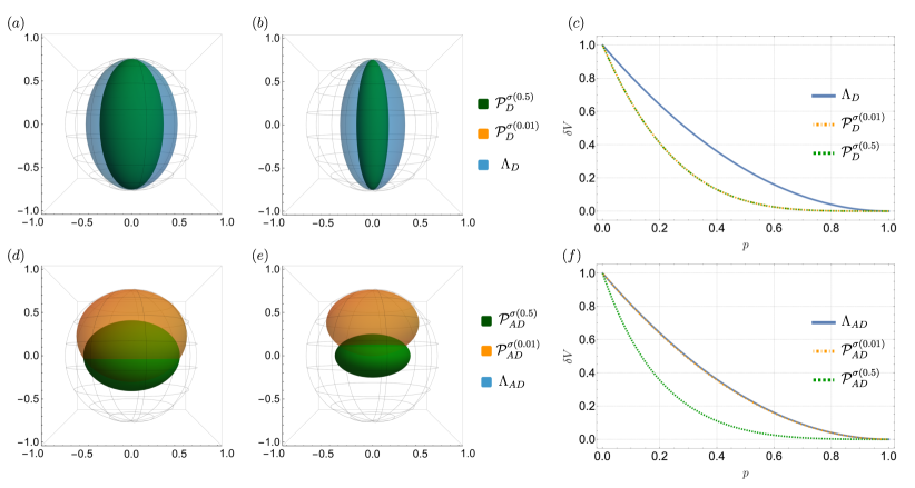
Figure 1: $(a)$ Set of accessible states under the action of the dephasing channel $\Lambda_{D}$ (blue ball) and the corresponding Petz recovery map for $\sigma(0.5)$ (green ball) and $\sigma(0.01)$ (orange ball) with $p=0.3$. The sets of accessible states for the Petz map (green and orange ball) coincide for both choices of reference states. $(b)$ Now fixing $p=0.5$. $(c)$ Volume $\delta V$ of accessible states for the dephasing channel $\Lambda_{D}$ (blue line) and its corresponding Petz recovery map $\mathcal{P}_{D}^{\sigma(0.01)}$ (orange dashed-dotted line) and $\mathcal{P}_{D}^{\sigma(0.5)}$ (green dashed line) in terms of the noise strength $p$. $(d)$ Set of accessible states under the action of the amplitude-damping channel $\Lambda_{AD}$ (blue ball) and the corresponding Petz recovery map for $\sigma(0.5)$ (green ball) and $\sigma(0.01)$ (orange ball) with $p=0.3$. The sets of accessible states for the $\Lambda_{AD}$ and $\mathcal{P}_{AD}^{\sigma(0.01)}$ (green and blue ball) coincide. $(e)$ Now fixing $p=0.5$. $(f)$ Volume $\delta V$ of accessible states for the amplitude-damping channel $\Lambda_{AD}$ (blue line) and its corresponding Petz recovery map $\mathcal{P}_{AD}^{\sigma(0.01)}$ (orange dashed-dotted line) and $\mathcal{P}_{AD}^{\sigma(0.5)}$ (green dashed line) in terms of the noise strength $p$.

III Geometrical characterization for the Petz recovery maps

Let us now look into certain geometrical features of the Petz map. To this end, we restrict our analysis to qubits. We investigate how the set of qubit states vary under the action of a quantum channel and its corresponding Petz recovery map. The resulting sets of evolved states $\rho^{\prime}=\{\Lambda(\rho)|\rho\in\mathcal{D}(\mathcal{H})\}$ and $\rho_{\mathcal{P}}=\{\mathcal{P}^{\sigma}(\Lambda(\rho))|\rho\in\mathcal{D}(\mathcal{H}\}$ for the above-mentioned scenarios, is defined here by the set of accessible states.

For qubits, the Bloch vector is 3-dimensional. The state space of all qubit density operators is represented by a ball of unit radius about the origin of $\mathbb{R}^{3}$, called the Bloch ball. Each point $(r_{x},r_{y},r_{z})$ of this ball corresponds to a unique state of the qubit. From Eq. (5), one can note that the action of a CPTP map $\Lambda$ either rotates or shrinks the Bloch vector for unital maps along with a possible translation in the case of non-unital maps. Such transformations induce a change in the volume of the set of accessible states, quantified as $\delta V=|M|$. We indicate with $|M|$ the determinant of the matrix $M$. For any positive and trace-preserving map, this quantity decreases monotonically with the strength of the map Cirac08 .

Let us now study the geometrical aspects of the Petz recovery map for the dephasing channel on qubits. States lying on the $z$-axis of the Bloch ball are invariant under the action of the dephasing map. These are the well-known fixed points of the map, $\Lambda(\rho)=\rho$. The set of accessible states is $\{\rho(\vec{r^{\prime}}):\vec{r^{\prime}}=[(1-p)r_{x},(1-p)r_{y},r_{z}]^{T}\}$. To obtain the set of accessible states for the Petz recovery map, we consider the following parametrization for the reference state $\sigma$

$$\sigma(\epsilon)=(1-\epsilon)|0\rangle\langle 0|+\epsilon|1\rangle\langle 1|,$$ (14)

with $\epsilon\in[0,1]$, a parameter that determines where the reference state lies on the $z$-axis. Choosing $\sigma$ as in Eq. (14), we build a Petz map $\mathcal{P}_{D}^{\sigma}$ for the dephasing channel, such that the recovered state is given by $\rho_{\mathcal{P}}=\mathcal{P}^{\sigma}_{D}(\Lambda_{D}(\rho))$, for any initial state $\rho$. The corresponding Bloch vector $\vec{r}_{\mathcal{P}}$ is then written as

$$\begin{split}r_{\mathcal{P}_{x}}=&\,(1+p^{2}-2p)r_{x}\\ r_{\mathcal{P}_{y}}=&\,(1+p^{2}-2p)r_{y}\\ r_{\mathcal{P}_{z}}=&\,r_{z}.\end{split}$$ (15)

As expected, $\vec{r}_{\mathcal{P}}$ is independent of $\epsilon$. This issue was already discussed in Lea21 ; any reference state of the form of Eq. (14) is an optimal choice for $\mathcal{P}^{\sigma}_{D}$. As can be apprehended from Fig. 1 $(a)$ and $(b)$ there is no distinction between the sets of recovered states of the Petz map for the different reference states (the green and orange balls in the plot are overlapped). However, the set of accessible states of the Petz map is always smaller than the set of accessible states of the dephasing map. In Fig. 1 $(c)$, we observe how the volumes of accessible states decrease with the noise strength of the map $p$. For intermediate noise strengths the volume for $\mathcal{P}^{\sigma}_{D}$ decreases faster than for $\Lambda_{D}$. They coincide in the extreme points when $p=0$ and $p=1$.

It is worth mentioning that the set of accessible states of the Petz map is obtained by acting the recovery map on a subset $\mathcal{S}(\mathcal{H})$ of the full set of one-qubit states, Eq. (11). In other words, the Petz map does not act over the full state space $\mathcal{D}(\mathcal{H})$. The bigger the set of accessible recovered states is, the better the access the Petz map has on $\mathcal{D}(\mathcal{H})$. However, it is worth pointing out that the volume of accessible states is not the only feature we should take into consideration when talking about state recoverability. In an optimal scenario, i.e. perfect recoverability, the set of accessible states for the Petz map should coincide with the set of accessible states of the decoherence channel.

Moving to the non-unital case, under the action of the amplitude damping channel, the set of accessible states is $\{\rho(\vec{r^{\prime}}):\vec{r^{\prime}}=[\sqrt{1-p}\,r_{x},\sqrt{1-p}\,r_{y},(1-p)\,rz+p\,\tau_{z}]^{T}\}$. Observe the shift in the $z$-direction, given by the translation component $\tau_{z}$. Taking the reference state of the form of Eq. (14), we obtain the corresponding Petz recovered states for the amplitude damping channel $\mathcal{P}^{\sigma}_{AD}$, whose Bloch vector is

$$\begin{split}r_{\mathcal{P}_{x}}=&\frac{\sqrt{1-\epsilon}\sqrt{|1-p|}}{\sqrt{1-\epsilon(1-p)}}\,r_{x},\text{ }r_{\mathcal{P}_{y}}=\frac{\sqrt{1-\epsilon}\sqrt{|1-p|}}{\sqrt{1-\epsilon(1-p)}}\,r_{y}\\ r_{\mathcal{P}_{z}}=&\frac{1-\epsilon+\epsilon p-p}{1-\epsilon(1-p)}\,r_{z},\text{ }\tau_{\mathcal{P}_{z}}=\frac{p(1-2\epsilon)}{1-\epsilon(1-p)}.\end{split}$$ (16)

The Petz map is now a non-unital map, depending on the choice of $\epsilon$ and $p$. From Eq. (16), we see that the recovered state depends not only on the strength of the map, given by $p$, but also on the choice of the reference state, given by $\epsilon$, contrary to what was observed in Eq. (15) for the dephasing channel. Again we choose two specific reference states: $\sigma(0.5)$ corresponds to the maximally mixed state and $\sigma(0.01)$ is a mixed state close to the fixed point of the map $|0\rangle\langle 0|$ footnote_1 . In Fig. 1 $(d)$ and $(e)$, we observe how for $\sigma(0.5)$, the set of accessible states for $\mathcal{P}^{\sigma}_{AD}$ (orange ball) is much smaller than the one for $\sigma(0.01)$ (green ball). It is also noticeable that $\mathcal{P}^{\sigma(0.01)}_{AD}$ is non-unital and its corresponding set of accessible states is shifted on the $z-$axis by $\tau_{\mathcal{P}_{z}}=0.296$ and $\tau_{\mathcal{P}_{z}}=0.492$ as in Figs. 1 $(d)$ and $(e)$, respectively. However, independently of the noise strength of the map, $\mathcal{P}^{\sigma(0.5)}_{AD}$ is always a unital map, from Eq. (16), we obtain $\tau_{\mathcal{P}_{z}}=0$. The sets of accessible states for $\Lambda_{AD}$ and $\mathcal{P}^{\sigma(0.01)}_{AD}$ are superposed, meaning that they coincide for all the points of the ball (the blue and orange balls coincide). In Fig. 1 $(f)$, we observe how the volume of accessible states for the Petz map decreases faster by choosing $\sigma$ as the maximally mixed state. On the contrary, taking $\sigma$ as a state close to the fixed point of the map, the volume decreases at the same rate as the map itself. Both reference states show an interesting property. The maximally mixed state is the trivial choice when dealing with recovery strategies, however, it is not as effective as the fixed point of the map for intermediate noise strengths  Lea21 . We provid a visual tool for the framework developed in  Lea21 and by observing these results, we conclude that the set of accessible states $\{\rho_{\mathcal{P}}\}$ reflects on the performance of the Petz map. A larger set of accessible states means a smaller compression of the domain, which is an advantage for the recovery map. Besides, we showed that the fixed point of the map is always a good choice for $\sigma$ when dealing with the full state space as an input. Unfortunately, the volume of accessible states is not the most appropriate figure of merit when moving to higher dimensions. Besides the increase in the computational cost, a geometrical visualization of the state space in higher dimensions turns out to be quite complicated and it is still an open question Kimura ; Krammer . In the next section, we develop a different framework employing the Choi matrices to explore if the dimension plays a role in the recovery strategy via the Petz maps.

IV Scalability of the Petz maps

We now attempt to investigate the performance of the Petz recovery maps for higher dimensions, via a state-independent figure of merit. Ideally, if the Petz map is capable of recovering the initial state $\rho$, we would obtain $\mathcal{P}^{\sigma}\Lambda(\rho)=\rho$, which implies

$$\mathcal{P}^{\sigma}\Lambda=\mathcal{I},$$ (17)

where $\mathcal{I}$ is the identity channel. In order to check the validity of Eq. (17), we propose a measure of distance between maps, given by

$$D(\mathcal{P}^{\sigma}\Lambda,\mathcal{I})=||J(\mathcal{P}^{\sigma}\Lambda)-J(\mathcal{I})||_{1},$$ (18)

where $J(\Lambda)$ is the Choi matrix corresponding to $\Lambda$. A map $\Lambda$ has an inverse $\Lambda^{-1}$ if $\Lambda^{-1}(\Lambda(\rho))=\rho,\,\forall\rho\in\mathcal{D}(\mathcal{H})$. The measure above reflects how far the Petz map is from the inverse of the map $\Lambda^{-1}$. If $\mathcal{P}^{\sigma}=\Lambda^{-1}$, $D(\mathcal{P}^{\sigma}\Lambda,\mathcal{I})=0$. The inverse map is usually not completely positive unless the original map is a unitary jagadish_measure2_2019 .

The measure above is well-behaved and bounded by Wallman

$$\frac{1}{d}||\Lambda_{1}-\Lambda_{2}||_{\diamond}\leq||J(\Lambda_{1})-J(\Lambda_{2})||_{1}\leq||\Lambda_{1}-\Lambda_{2}||_{\diamond},$$ (19)

with $||\Lambda||_{\diamond}\equiv\text{max}_{\rho}||(\mathbb{1}\otimes\Lambda)\rho||_{1}$ being the diamond norm. The channels are perfectly distinguishable if $||\Lambda_{1}-\Lambda_{2}||_{\diamond}=2$. Observe that the measure proposed in Eq. (18) can be more easily calculated, since it does not require an optimization as the diamond norm. This strategy provides a state-independent framework, which can be quite useful and has a lower computational cost when increasing the dimension. To obtain the Petz recovery map, we extend the parametrization from Eq. (14) to the $d$-dimensional scenario

$$\sigma(\epsilon)=(1-\epsilon)|0\rangle\langle 0|+\frac{\epsilon}{d-1}\sum_{n=1}^{d}|n\rangle\langle n|,$$ (20)

with $\epsilon\in[0,1]$.

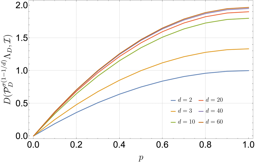
Figure 2: Distance between the Petz map applied to the dephasing channel and the identity channel, $D(\mathcal{P}_{D}^{\sigma(1-1/d)}\Lambda_{D},\mathcal{I})$, versus the noise strength $p$ for different dimensions.

For the dephasing channel, we fix the reference state as the maximally mixed one, $\sigma(1-1/d)$. A plot of the distance $D(\mathcal{P}_{D}^{\sigma(1-1/d)}\Lambda_{D},\mathcal{I})$ versus $p$ for different dimensions $d$ is shown in Fig. 2 . We observe that the displacement between the curves decreases with increase in dimensions and is getting much smaller as we move towards $D(\mathcal{P}_{D}^{\sigma(1-1/d)}\Lambda_{D},\mathcal{I})=2$. In order to verify if this bound is saturated for a certain dimension $d=n$, in Fig. 3 we plot $D(\mathcal{P}_{D}^{\sigma(1-1/d)}\Lambda_{D},\mathcal{I})$ versus the dimension fixing $p=1$ (maximum noise). As expected and previously discussed, the distance between the two maps stabilizes when increasing the dimension. As an example, taking $d=20$ we obtain $D(\mathcal{P}_{D}^{\sigma(1-1/d)}\Lambda_{D},\mathcal{I})=1.90$, for $d=40$, $D(\mathcal{P}_{D}^{\sigma(1-1/d)}\Lambda_{D},\mathcal{I})=1.95$ and for $d=60$, $D(\mathcal{P}_{D}^{\sigma(1-1/d)}\Lambda_{D},\mathcal{I})=1.97$.

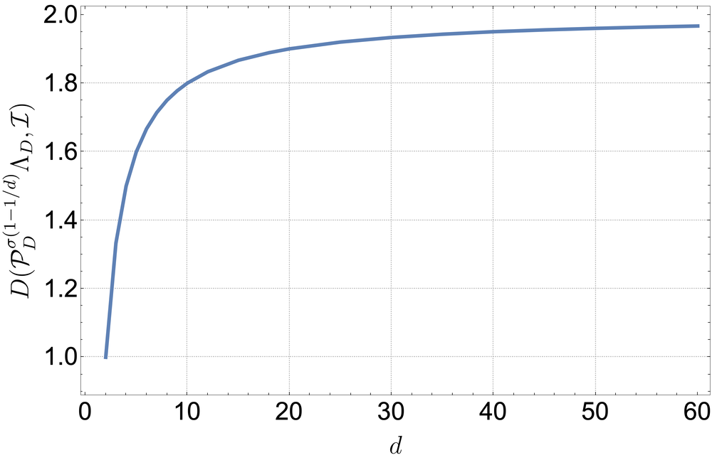
Figure 3: Distance between the Petz map applied to the dephasing channel and the identity channel, $D(\mathcal{P}_{D}^{\sigma(1-1/d)}\Lambda_{D},\mathcal{I})$, versus the dimension $d$ for $p=1$ (maximum noise).

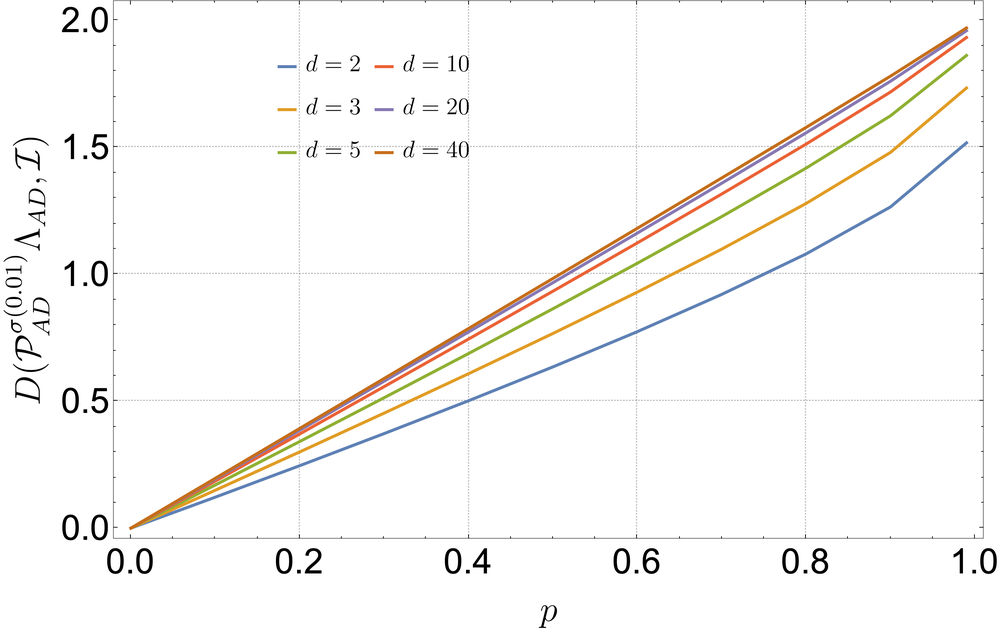
Figure 4: Distance between the Petz map applied to the amplitude-damping channel and the identity channel, $D(\mathcal{P}_{AD}^{\sigma(0.01)}\Lambda_{AD},\mathcal{I})$, versus the noise strength $p$ for different dimensions.

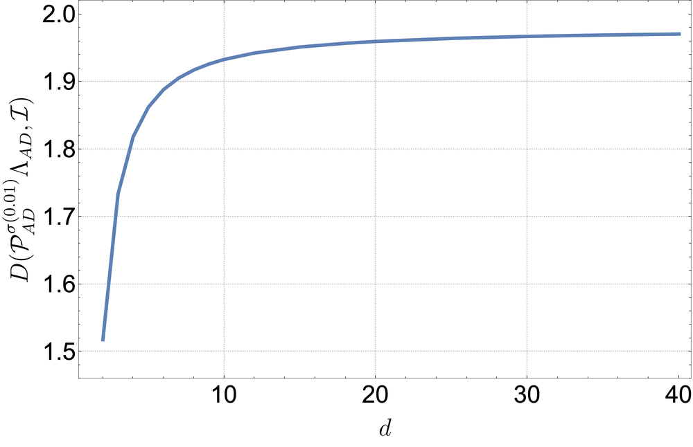
Figure 5: Distance between the Petz map applied to the amplitude-damping channel and the identity channel, $D(\mathcal{P}_{AD}^{\sigma(0.01)}\Lambda_{AD},\mathcal{I})$, versus the dimension $d$ for $p=1$ (maximum noise).

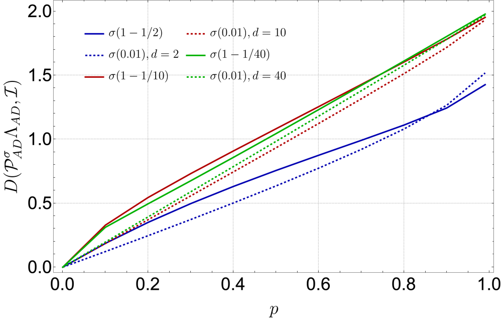
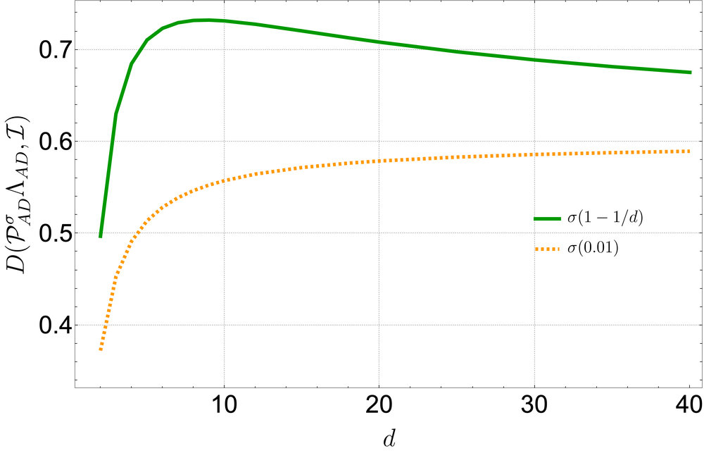
Figure 6: Distance between the Petz map applied to the amplitude-damping channel and the identity channel, $D(\mathcal{P}_{AD}^{\sigma}\Lambda_{AD},\mathcal{I})$. On the left, the difference between the choice of the reference state was exploited for dimensions $d=2,10,\text{and }40$ in terms of noise parameter $p$. For each dimension, the reference state analyzed is the corresponding maximally mixed state, $\sigma(1-1/d)$, and a reference state close to the fixed point of the map, $\sigma(0.01)$. On the right, $D(\mathcal{P}_{AD}^{\sigma}\Lambda_{AD},\mathcal{I})$ for $p=0.3$ versus the dimension $d$.

For the amplitude damping channel, a similar behavior can be observed. Initially, we decided to fix the reference state close to the fixed point, $\sigma(0.01)$. In Fig. 4 we observe how the distance $D(\mathcal{P}_{AD}^{\sigma(0.01)}\Lambda_{AD},\mathcal{I})$ increases with the dimension. Again, the curves are getting closer for higher dimensions. This can be easily seen in Fig. 5. Fixing the noise strength at $p=1$, a plateau is achieved and the performance of the Petz recovery map will be the same for $d\geq 12$, since $D^{\prime}(\mathcal{P}_{AD}^{\sigma(0.01)}\Lambda_{AD},\mathcal{I})=0$, where $D^{\prime}(\mathcal{P}_{AD}^{\sigma(0.01)}\Lambda_{AD},\mathcal{I})$ is the derivative of the curve displayed in Fig. 5. If we consider now the reference as being the maximally mixed state $\sigma(1-1/d)$ for intermediate noise strengths, we observe an advantage for $d=40$ over $d=10$ in Fig. 6 (left). The green and red solid lines cross at $p=0.75$. To understand if the dimension plays a role in the performance of the Petz recovery map, in Fig. 6 (right), we plot the distance versus the dimension for different choices of the reference state. We see that for an intermediate noise strength, $p=0.3$, the advantage of choosing $\sigma$ close to the fixed point of the map is clear. However, when choosing $\sigma(1-1/d)$, dimension comes into play and impacts the recovery performance. We obtain for $d=10$ and $d=40$, $D(\mathcal{P}_{AD}^{\sigma(0.5)}\Lambda_{AD},\mathcal{I})=0.73$ and $D(\mathcal{P}_{AD}^{\sigma(0.5)}\Lambda_{AD},\mathcal{I})=0.68$, respectively.

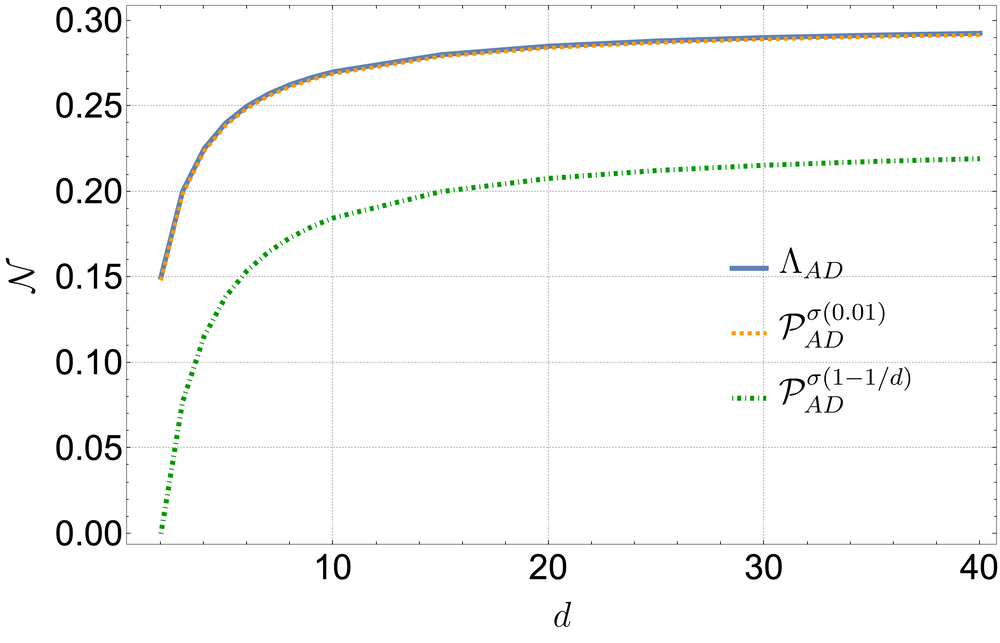
Figure 7: Non-unitality measure $\mathcal{N}$ in terms of the dimension, fixing $p=0.3$, for the amplitude-damping channel (thick) and its corresponding Petz map for $\sigma(0.01)$ (dashed) and $\sigma(1-1/d)$ (dot-dashed).

To clarify the role of the dimension in the state recovery via the Petz map, we also compute the non-unitality measure, $\mathcal{N}$, introduced in Sec.II. As can be seen from Fig. 7, for $p=0.3$, the non-unitality measure $\mathcal{N}$ for the Petz map increases with the dimension but the outcome is different depending on the choice of the reference state. We observe that the curves for $\mathcal{P}_{AD}^{\sigma(0.01)}$ and $\Lambda_{AD}$ are superposed, meaning that the Petz map for the choice of $\sigma(0.01)$ shifts the maximally mixed state in the same way as the amplitude-damping channel. On the other hand, for $\mathcal{P}_{AD}^{\sigma(1-1/d)}$, $\mathcal{N}$ is much smaller and it does not reproduce the same non-unital behavior as $\Lambda_{AD}$. This has already been discussed in Sec. III. Changing the noise strength $p$, the same behavior of $\mathcal{N}$ is observed but with different values. For a qubit, from Fig. 7, we obtain $\mathcal{N}=0$ and $\mathcal{N}=0.15$ for the choices of $\sigma(1-1/d)$ and $\sigma(0.01)$, respectively. Bringing together Figs. 6 and 7, a connection can be traced. When choosing $\sigma(1-1/d)$, the Petz map does not retrieve the non-unital behavior of the amplitude damping, contrary to what is observed for the choice of $\sigma(0.01)$. This is a limitation that reflects on the bad performance of $\mathcal{P}_{AD}^{\sigma(1-1/d)}$ compared to $\mathcal{P}_{AD}^{\sigma(0.01)}$. However, when increasing the dimension, the measure $\mathcal{N}$ also increases, therefore decreasing the difference between the non-unital character of $\Lambda_{AD}$ and $\mathcal{P}_{AD}^{\sigma(1-1/d)}$. Consequently, the recovery is improved, as can be observed in Fig. 6 (right).

V Conclusions

In the present work, we analyze the geometrical aspects of the Petz recovery maps for qubit channels. We have shown how the volume of accessible states can be directly linked to the recoverability property of the Petz map. The similar the volumes of accessible states for the evolved states and the recovered states are, the better the performance of the Petz map. This result is particularly relevant when considering the choice of reference state, as discussed also in Lea21 .

In addition, we have developed a state-independent framework for Petz maps for qudits, which extends our analysis to arbitrary dimensions. While the complete characterization of the optimal recovery map is a non-trivial problem in higher dimensions, we used the distance measure based on the Choi-Jamiołkowski isomorphism. Our findings emphasize the importance of carefully selecting the reference state for the Petz map. Moreover, we have identified that for non-unital maps, the non-unitality measure for the Petz map is not the same as the one for the corresponding quantum channel. However, the Petz map and the original map tend to be equally non-unital when increasing the dimensions.

Our work provides a novel approach to understanding and characterizing the Petz recovery maps, that has the potential to improve quantum information processing protocols. We anticipate that the insights gained about the characteristics and performance of Petz recovery maps can provide valuable guidance in designing quantum error correction protocols that are more effective and applicable to a wide range of quantum systems.

Appendix A Non-uniform amplitude damping channel

We also investigate if changes in the recoverability can be observed in the case of non-uniform amplitude damping, i.e. when different damping rates are considered. Let us take the qutrit case as an example. The Kraus operators are known from Eq. (II.1.2), but now with a slight modification;

$$K_{0} = |0\rangle\langle 0|+\sqrt{1-p_{1}}|1\rangle\langle 1|+\sqrt{1-p_{2}}|2\rangle\langle 2|$$

$$K_{1} = \sqrt{p_{1}}|0\rangle\langle 1|$$

$$K_{2} = \sqrt{p_{2}}|0\rangle\langle 2|,$$ (21)

with $p_{1},p_{2}\in[0,1]$ being the decay probabilities. In the non-uniform case, these probabilities assume different values, which allows us to deal with a more realistic scenario. In Fig.  8 we plot the behavior of the distance defined in Eq. (18), in terms of $p_{1}$ and $p_{2}$.

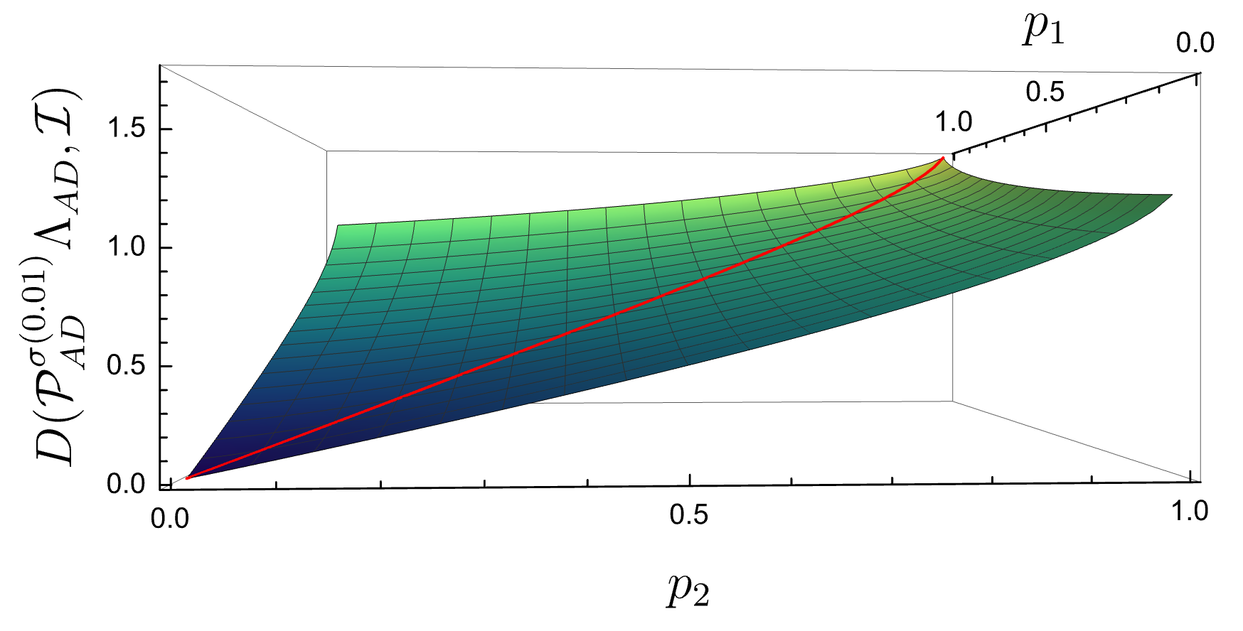
Figure 8: Distance between the Petz map applied to the amplitude-damping and the identity channel in terms of the decay probabilities $p_{1}$ and $p_{2}$. The red curve corresponds to the uniform case, $p_{1}=p_{2}$.

We can see that the distance for the uniform amplitude damping (diagonal red curve) turns out to be smaller than for the non-uniform scenario. When the decay probabilities are equal, a better recovery is observed for the Petz map. Assuming that one of the probabilities is zero, the system reduces to a two-level system, and we recover the result displayed in Fig. 4 of the main text for $d=2$.

References

- (1) John D. Norton. The Impossible Process: Thermodynamic Reversibility. Stud. Hist. Philos. Sci. B - Stud. Hist. Philos. Mod. Phys. 55: 43-61 (2016)
- (2) Heinz-Peter Breuer and Francesco Petruccione. The Theory of Open Quantum Systems. (Oxford University Press, Oxford, 2002).
- (3) Ángel Rivas and Susana F. Huelga. Open Quantum Systems: An Introduction. (Springer Berlin, Heidelberg, 2012).
- (4) Serge Haroche and Jean Michel Raimond. Exploring the Quantum: Atoms, Cavities, and Photons. (Oxford University Press, Oxford, 2006).
- (5) Vinayak Jagadish and Francesco Petruccione. An invitation to quantum channels. Quanta 7(1):54–67 (2018).
- (6) Dénes Petz. Sufficient subalgebras and the relative entropy of states of a von Neumann algebra. Commun. Math.Phys. 105, 123-131 (1986).
- (7) Dénes Petz. Sufficiency of channels over von Neumann algebras. Quart. J. Math.Oxford Ser. (2), 39,01 (1988).
- (8) Dénes Petz. Monotonicity of quantum relative entropy revisited. Rev. Math. Phys. 15,01 (2003).
- (9) Marius Junge, Renato Renner, David Sutter, Mark M. Wilde, and Andreas Winter. Universal Recovery Maps and Approximate Sufficiency of Quantum Relative Entropy. Ann. Henri Poincaré 19(10):2955–2978, (2018).
- (10) Howard Barnum and Emanuel Knill. Reversing quantum dynamics with near-optimal quantum and classical fidelity. J. Math. Phys. 43(5):2097–2106, (2002).
- (11) Francesco Buscemi and Valerio Scarani. Fluctuation theorems from Bayesian retrodiction. Phys. Rev. E 103(5): 052111 (2021).
- (12) Clive Cenxin Aw, Francesco Buscemi, and Valerio Scarani. Fluctuation theorems with retrodiction rather than reverse processes. AVS Quantum Sci. 3(4): 045601 (2021).
- (13) Hyukjoon Kwon, Rick Mukherjee, and M.S. Kim. Reversing Lindblad Dynamics via Continuous Petz Recovery Map. Phys. Rev. Lett. 128, 020403 (2022).
- (14) András Gilyén, Seth Lloyd, Iman Marvian, Yihui Quek, and Mark M. Wilde. Quantum Algorithm for Petz Recovery Channels and Pretty Good Measurements Phys. Rev. Lett. 128, 220502 (2022)
- (15) Lea Lautenbacher, Fernando de Melo, and Nadja K. Bernardes. Approximating invertible maps by recovery channels: Optimality and an application to non-Markovian dynamics. Phys. Rev. A 105, 042421 (2022).
- (16) Jacopo Surace and Matteo Scandi. State retrieval beyond Bayes’ retrodiction and reverse processes. Quantum 7, 990 (2023).
- (17) Karol Życzkowski and Hans-Jürgen Sommers. Average fidelity between random quantum states. Phys. Rev. A 71, 032313 (2005).
- (18) Man-Duen Choi. Completely positive linear maps on complex matrices. Linear Algebra Appl. 10, 285 (1975).
- (19) Andrzej Jamiołkowski. Linear transformations which preserve trace and positive semidefiniteness of operators. Rep. Math. Phys. 3 (4): 275–278 (1972).
- (20) Michael M. Wolf and Ignacio J. Cirac. Dividing Quantum Channels. Commun. Math. Phys. 279(1):147–168 (2008).
- (21) The choice is based on the fact that the results converge for .
- (22) Gen Kimura. The Bloch Vector for N-Level Systems. Phys. Lett. A 314, 339 (2003).
- (23) Reinhold A Bertlmann and Philipp Krammer. Bloch vectors for qudits. J. Phys. A: Math. Theor. 41 235303 (2008).
- (24) Vinayak Jagadish, R. Srikanth, and Francesco Petruccione. Measure of not-completely-positive qubit maps: The general case. Phys. Rev. A 100, 012336 (2019).
- (25) Joel J. Wallman and Steven T. Flammia. Randomized benchmarking with confidence. New J. Phys. 16, 103032 (2014).