Applying Ising Machines to Multi-objective QUBOs

Abstract

Multi-objective optimisation problems involve finding solutions with varying trade-offs between multiple and often conflicting objectives. Ising machines are physical devices that aim to find the absolute or approximate ground states of an Ising model. To apply Ising machines to multi-objective problems, a weighted sum objective function is used to convert multi-objective into single-objective problems. However, deriving scalarisation weights that archives evenly distributed solutions is not trivial. Previous work has shown that adaptive weights based on dichotomic search, and one based on averages of previously explored weights can explore the Pareto front quicker than uniformly generated weights. However, these adaptive methods have only been applied to bi-objective problems in the past. In this work, we extend the adaptive method based on averages in two ways: (i) we extend the adaptive method of deriving scalarisation weights for problems with two or more objectives, and (ii) we use an alternative measure of distance to improve performance. We compare the proposed method with existing ones and show that it leads to the best performance on multi-objective Unconstrained Binary Quadratic Programming (mUBQP) instances with 3 and 4 objectives and that it is competitive with the best one for instances with 2 objectives.

Keywords Digital Annealer, QUBO, Multi-objective optimisation, Adaptive Scalarisation

Keywords Multi-objective, Quadratic Unconstrained Binary Optimisation, Digital Annealer, Adaptive Scalarisation, Adaptive Aggregation

1 Introduction

Multi-objective optimisation problems have multiple and often conflicting objectives. The goal of multi-objective optimisation is to find the Pareto front (PF). The PF is the set of solutions where no other feasible solution can improve on at least one objective without sacrificing the performance of at least one other objective.

Unconstrained Binary Quadratic Programming (UBQP) problems also known as Quadratic Unconstrained Binary Optimisation (QUBO) problems have been widely studied. QUBO is of particular interest within the context of Ising machines because combinatorial optimisation problems can be formulated as QUBO, allowing Ising machines to be applied to a wide range of practical problems. Many practical problems naturally have multiple and often conflicting objectives e.g. the Cardinality Constrained Mean-Variance Portfolio Optimisation Problem (CCMVPOP) (Chang et al., 2000) which entails minimising risks while maximising returns. Ising machines such as Fujitsu’s Digital Annealer (DA) (Hiroshi et al., 2021) and D-wave’s Quantum Annealer (QA) (McGeoch and Farré, 2020) are however single-objective solvers. To apply Ising machines to multi-objective problems, the problem needs to be converted to a single-objective problem.

Scalarisation by means of weighted sum is a common approach for transforming multi-objective problems into single-objective ones, allowing the application of single-objective solvers. The scalarisation weights play a critical role in determining the balance between the objectives and must be chosen carefully to achieve evenly distributed solutions around the PF. Several methods for deriving scalarisation weights have been proposed in previous work.

In previous work applying Ising machines to multi-objective problems, scalarisation weights were derived experimentally, using problem-specific knowledge, uniformly generated weights, or adaptively generated weights. For example, scalarisation weights were derived experimentally (Elsokkary et al., 2017) or using problem-specific knowledge (Phillipson and Bhatia, 2021) when QA was applied to multi-objective portfolio optimisation problems. Scalarisation weights were also derived experimentally when a QA-inspired algorithm was applied to the problem of designing analog and mixed-signal integrated circuits (Martins et al., 2021). Ayodele et al. (2022) proposed an adaptive method (referred to as an iterative method) for the CCMVPOP, which they compared with randomly and uniformly generated weights. The adaptive method derives new weights by calculating the average of a pair of previously explored scalarisation weights. The pair of weights selected are those that lead to the solutions with the highest Manhattan distance between their objective function values. Ayodele et al. (2022) showed that a higher hypervolume (Zitzler and Thiele, 1998) (Section 4.3.2), a popular algorithm performance metric in multi-objective optimisation, was achieved when compared to uniformly or randomly generated weights. The improved performance of the adaptive method is consistent with previous findings based on classical algorithms. For example, a dichotomic procedure that derives new weights perpendicular to two solutions in the objective space that have the largest Euclidean distance between them was applied to the bi-objective traveling salesman problem (Dubois-Lacoste et al., 2011), bi-objective permutation flow-shop scheduling problem (Dubois-Lacoste et al., 2011) and bi-objective UBQP (Liefooghe et al., 2015). This adaptive method is shown to have better anytime behaviour when compared to uniformly generated weights. This means that the adaptive approach can deliver a good performance even with a small number of weights.

These adaptive methods have only been applied to bi-objective problems. The higher the number of objectives, the higher the number of weights typically needed to reach a good PF representation. Therefore, it becomes important to explore better techniques for deriving scalarisation weights for problems with more than two objectives. In this work, we extend the adaptive method in (Ayodele et al., 2022) in the following ways:

• We extend the approach for more than 2 objectives,

• We consider replacing the Manhattan distance metric with Euclidean distance,

• We experiment with the proposed approach on mUBQP instances with 2, 3, and 4 objectives.

To assess the performance of the proposed adaptive method, we compare it to other scalarisation techniques: uniformly generated weights based on Maximally Dispersed Set (MDS) of weights (also known as the simplex lattice design) proposed by Steuer (1986), an adaptive method based on dichotomic search and Euclidean distance (Dubois-Lacoste et al., 2011) (for 2 objectives only) and an adaptive method based on average weights and Manhattan distance (Ayodele et al., 2022). To be consistent with the term used in recent work, we will refer to the MDS as simplex lattice design for the rest of this work. To achieve a fair comparison, the same single-objective solver (DA) is used within the scalarisation frameworks. Moreover, although the DA has been used in this study as the underlying Ising machine, the scalarisation methods are applicable to any Ising machine.

The rest of this work is structured as follows. The mUBQP problem formulation is presented in Section 2. The techniques of deriving scalarisation weights are presented in Section 3. Parameter settings and the considered mUBQP instances are presented in Section 4. Results and conclusions are presented in Sections 5 and 6.

2 Multi-objective Unconstrained Binary Quadratic Programming

The multi-objective UBQP (mUBQP) is formally defined as (Liefooghe et al., 2014):

$$c_{k}(x) =\sum_{i=1}^{n}\sum_{j=1}^{n}Q_{ijk}x_{i}x_{j}\quad k\in\{1,2,\dotsc,m\}\;,$$ (1)

s.t. $$x\in\{0,1\}^{n}\;,$$ (2)

where $Q$ is a 3-dimensional matrix consisting of $m$ number of $n\times n$ QUBO matrices, $m$ is the number of objectives, $c=(c_{1},\dots,c_{m})$ is an objective function vector and $n$ is the problem size (number of binary variables).

We combine the objectives using a vector of scalarisation weights $\boldsymbol{\lambda}=\left(\lambda_{1},\dots,\lambda_{m}\right)$, such that, $\sum_{j=1}^{m}\lambda_{j}=1$. The aim is to minimise the energy $E(x)$ defined as:

Minimise $$E(x)=\lambda_{1}\cdot c_{1}(x)+\dots+\lambda_{m}\cdot c_{m}(x)\;$$ (3)

3 Scalarisation Methods for QUBO solving

In this section, we present the Ising machine as well as scalarisation techniques used in this work.

3.1 Digital Annealer

Fujitsu’s DA belongs to the category of Ising machines and has evolved over the years, from the $1^{\text{st}}$ and $2^{\text{nd}}$ generation, which is capable of solving QUBO problems of up to 1,024 bits and 8,192 bits, respectively, to the $3^{\text{rd}}$ and $4^{\text{th}}$ generations, which are able to solve Binary Quadratic Problems (BQPs) with up to 100,000 bits. Although the $3^{\text{rd}}$ and $4^{\text{th}}$ generation DAs have more capabilities than previous generations such as automatic tuning of constraint coefficients, the ability to handle inequality constraints, and a higher number of bits, these capabilities were not needed for the mUBQP instances used in this study. We, therefore, use the $2^{\text{nd}}$ generation DA. More details about the DA are presented in (Hiroshi et al., 2021; Matsubara et al., 2020). In the rest of this work, DA will be used to refer to the $2^{\text{nd}}$ generation DA.

3.2 Scalarisation Methods

In this section, we present the scalarisation techniques used in this work.

• Uniformly generated weights based on simplex lattice design (Zhou et al., 2018) (Section 3.2.1)

• an adaptive method based on dichotomic search (Dubois-Lacoste et al., 2011) (Section 3.2.2)

• proposed extension of the adaptive method based on averages proposed in (Ayodele et al., 2022) (Section 3.2.3)

We note that the frameworks can be used for other Ising machines by replacing the DA with another Ising machine.

Algorithm 1 Uniform Method based on Simplex Lattice Design

1:$P$, n_weights, alg_parameters

2:$\Lambda\leftarrow\textit{SimplexLatticeDesign}(H,m)$

3:$A\leftarrow\emptyset$$\triangleright$ Initialise archive

4:for each $\boldsymbol{\lambda}=\left(\lambda_{1},\dots,\lambda_{m}\right)\in\Lambda$ do$\triangleright$ In any arbitrary order

5:     $Q$ $\leftarrow$$sum(P_{j}\cdot\lambda_{j}\ \forall\ j\in\left\{1,\dots,m\right\})$

6:     $Y\leftarrow$ Solver($Q$, alg_parameters)

7:     add all solutions in $Y$ to $A$

8:end for

9:return all non-dominated solutions from archive $A$

3.2.1 Uniform Weights: Simplex Lattice Design

Algorithm 1 presents a scalarisation technique that utilises uniformly distributed scalarisation weights. Such evenly distributed weights are generated using the simplex lattice design. The required parameters are $P$, the list of QUBOs representing all the objectives, n_weights, number of weights, and alg_parameters, a set of parameters used by the Ising Machine of choice (DA). Parameters used in this work are presented in Table 1. The simplex lattice design is a common approach for generating evenly distributed weights when solving multi-objective problems with scalarisation techniques (Zhou et al., 2018; Chen et al., 2022; Zhang and Li, 2007). The simplex lattice design consists of two parameters $H$ and $m$ (Algorithm 1, line 2). A simplex-lattice mixture design of degree $H$ consists of $H+1$ points of equally spaced values between 0 and 1 for each objective, while $m$ is the number of objectives. The possible scalarisation weights will be taken from $\left\{\frac{0}{H},\frac{1}{H},\dots,\frac{H}{H}\right\}$. These weights are combined such that they sum to 1. The number of scalarisation weight vectors that can be generated using this approach is $\binom{H+m-1}{m-1}=\frac{(H+m-1)!}{H!(m-1)!}$; e.g if $m=2$ and $H=3$, the number of weights is 4 which are $\left[\left(0.00,1.00\right),\left(0.33,0.67\right),\left(0.67,0.33\right),\left(1.00,0.00\right)\right]$. To achieve 10 weights used in this study $H=9$, $3$ or $2$ when $m=2$, $3$ or $4$, respectively (Algorithm 1, line 2).

The solver (DA) is applied to a weighted aggregate (Algorithm 1, line 6) of the QUBOs representing all objectives. DA returns a set of more promising solutions by default. All of these are added to the archive ($A$). The final step (Algorithm 1, line 9) entails filtering $A$ such that only the non-dominated solutions are returned. A solution is non-dominated if there is no other solution that is better in one objective without being worse in another objective.

3.2.2 Adaptive Weights - Dichotomic Search

Scalarisation technique based on dichotomic search is presented in Algorithm 2. In addition to parameters ($P$, n_weights, alg_parameters) used in Section 3.2.1, a parameter $dm$, metrics, is also used. This method is initialised with a set of weights $\Lambda$ that minimise each individual objective (e.g $\left[\left(0.00,1.00\right),\left(1.00,0.00\right)\right]$ for two objectives or $\left[\left(0.00,0.00,1.00\right),\left(0.00,1.00,0.00\right),\left(1.00,0.00,0.00\right)\right]$ for three objectives). Once these weights are exhausted, new weights are derived adaptively by targeting the largest gap within the set of solutions found. The largest gap between each pair of solutions is measured in the objective space based on the selected $dm$; i.e Euclidean distance. The differences in cost function values that correspond to the largest gap are used to derive new weights for the next iteration (Algorithm 2, lines 10–13). The difference in the first and second cost function values are normalised such that they sum to 1, and are used as the scalarisation weights for the second and first objective respectively. This method was designed for problems with two objectives only. The best solutions returned by the DA during each scalarisation are saved to the archive $A$ which are then filtered for non-dominated solutions.

Algorithm 2 Adaptive Method based on Dichotomic Search

1:$P$, n_weights, $dm=$ ‘Euclidean’, alg_parameters

2:$\Lambda\leftarrow\textit{SimplexLatticeDesign}(1,m)$ $\triangleright$ $H=1$

3:$A\leftarrow\emptyset$, $W\leftarrow\left\{\right\}$ $\triangleright$ Initialise archive and mapping between weights and cost functions

4:for each $i\in\left\{1,\dots,n\_weights\right\}$  do

5:     if $i\leq 2$ then

6:         $\boldsymbol{\lambda}=\left(\lambda_{1},\lambda_{2}\right)\leftarrow\Lambda_{i}$

7:     else

8:         sort $W$ by $c_{1}(x)$

9:         select 2 adjacent solutions ($y$ and $z$) from $W$, that lead to the largest $dm$ distance in objective space where $c_{1}(y)>c_{1}(z)$

10:         $temp\_\lambda_{1}$ $\leftarrow$$c_{2}(y)-c_{2}(z)$

11:         $temp\_\lambda_{2}$ $\leftarrow$$c_{1}(z)-c_{1}(y)$

12:         $sum\_\lambda\leftarrow temp\_\lambda_{1}+temp\_\lambda_{2}$

13:         $\boldsymbol{\lambda}\leftarrow\left(\left(\frac{temp\_\lambda_{1}}{sum\_\lambda}\right),\left(\frac{temp\_\lambda_{2}}{sum\_\lambda}\right)\right)$

14:     end if

15:     $Q\leftarrow(P_{1}\cdot\lambda_{1})+(P_{2}\cdot\lambda_{2})$

16:     $Y\leftarrow$ Solver($Q$, alg_parameters)

17:     add all solutions in $Y$ to $A$

18:     $W_{i}\leftarrow[x,\left(c_{1}(x),c_{2}(x)\right)]$ where $x=Y_{0}$$\triangleright$ save solution and cost function values for the best solution in $Y$

19:end for

20:return all non-dominated solutions from archive $A$

3.2.3 Adaptive Weights - Averages

The proposed extension to the adaptive method in (Ayodele et al., 2022) is presented in Algorithm 3. This adaptive method was originally proposed for QUBO formulations of the bi-objective Cardinality Constrained Mean-Variance Portfolio Optimisation Problem (CCMVPOP). In this work, we extend this adaptive approach for QUBO problems with more than two objectives. We also extend the distance metric $dm$ to include Euclidean distance. We note that only Manhattan distance was used in (Ayodele et al., 2022).

Similar to the adaptive method based on dichtomic search, parameters ($P$, n_weights, alg_parameters, $dm$) are used. This method is also initialised with a set of weights that minimise each individual objective independently. Once these weights are exhausted, new weights are derived adaptively by targeting the largest gap in the objective space (measured by the selected $dm\in\left\{Manhattan,Euclidean\right\}$) of the set of solutions found. The two weight vectors (corresponding to all objectives) that lead to the largest gap are averaged for each objective (Alg. 3, line 10) and used in subsequent iterations until the stopping criterion is met (i.e. n_weights is reached). The best solutions returned by the DA during each scalarisation are saved to the archive $A$. The filtered set of non-dominated solutions is returned as the final output (Alg. 3, line 20). Unlike the dichotomic method, this approach can be applied to any number of objectives.

Note that for all of the methods presented in this work, Solver refers to the DA while alg_parameters refers to DA parameters (Algorithm 1, line 6; Algorithm 2, line 2; Algorithm 3, line 14). In (Ayodele et al., 2022), a set of top solutions (solutions with lower energies/cost function) were considered for non-dominance. We use the same approach in this work since the DA returns a set of top solutions by default. To apply the presented methods using an alternative Ising machine, Solver will refer to such Ising machine.

Algorithm 3 Proposed Adaptive Method based on Averages

1:$P$, n_weights, alg_parameters, $dm\in$ [‘Euclidean’, ‘Manhattan’]

2:$\Lambda\leftarrow\textit{SimplexLatticeDesign}(1,m)$ $\triangleright$ $H$ is set to 1

3:$A\leftarrow\emptyset$, $W\leftarrow\left\{\right\}$ $\triangleright$ Initialise archive and mapping between weights and cost functions

4:for each $i\in\left\{1,\dots,n\_weights\right\}$  do

5:     if $i\leq m$ then

6:         $\boldsymbol{\lambda}=\left(\lambda_{1},\dots,\lambda_{m}\right)\leftarrow\Lambda_{i}$

7:     else

8:         sort $W$ by $\lambda$

9:         select two adjacent parent weight vectors $U$ and $V$ from $W$, that lead to the largest $dm$ distance in objective space

10:         $\boldsymbol{\lambda}\leftarrow\left(\frac{U_{1}+V_{1}}{2},\cdots,\frac{U_{m}+V_{m}}{2}\right)$

11:     end if

12:     $Q$ $\leftarrow$$sum(P_{j}\cdot\lambda_{j}\ \forall\ j\in\left\{1,\dots,m\right\})$

13:     $Y\leftarrow$ Solver($Q$, alg_parameters)

14:     add all solutions in $Y$ to $A$

15:     $W_{i}\leftarrow[\lambda,\left(c_{1}(x),\dots,c_{m}(x)\right)]$ where $x=Y_{0}$$\triangleright$ save weight vector and cost function values for the best solution in $Y$

16:end for

17:return all non-dominated solutions from archive $A$

4 Experimental Settings

In this section, we present the mUBQP instances, parameter settings and performance measures considered in this study.

4.1 Multi-objective Unconstrained Binary Quadratic Programming Instances

The mUBQP instances used in this study have been obtained and are available from mUBQP Library. The Library consists of instances with varying $\rho$-values (objective correlation coefficient), $m$ (number of objective functions), $n$ (length of bit strings), and $d$ the matrix density (the frequency of non-zero numbers). In this study, we use eleven instances with $n$ = 1000, varying $\rho\in\left\{-0.9,-0.2,0.0,0.2,0.5,0.9\right\}$, $m\in\left\{2,3\right\}$, $d\in\left\{0.4,0.8\right\}$. In order to experiment the proposed approach on instances with four objectives, we use the instance generator provided as part of the mUBQP Library using parameters $n=1000$, $\rho\in\left\{-0.2,0.2,0.5,0.9\right\}$, $m=4$, $d=0.8$ to generate four additional instances. All fifteen instances used in this study are made available.

4.2 Parameter Settings

Parameter settings used by DA are presented in Table 1. The DA is capable of executing multiple annealing methods in parallel. The number of parallel executions is controlled by the number of replicas parameter. Each replica executes for a given number of iterations, this is controlled by the number of iterations parameter. $T_{0}$ is the initial temperature used by the DA, the temperature is reduced at the rate specified by $\beta$ after every $I$ iteration(s). We use the exponential mode of reducing the temperature. The exponential mode calculates the temperature at each iteration based on the temperature at the previous iteration. The DA employs an escape mechanism called a dynamic offset, such that if a neighbour solution was accepted, the subsequent acceptance probabilities are artificially increased by subtracting a positive value from the difference in energy associated with a proposed move (Matsubara et al., 2020).

The number of weights (n_weights) explored by all methods is $10$. Where uniformly generated weights are used $H=9$ when $m=2$, $H=3$ when $m=3$ and $H=2$ when $m=4$.

Table 1: DA parameters.

Parameters	Values
Start Temperature ($T_{0}$)	$10^{4}$
Temperature Decay ($\beta$)	$0.2$
Temperature Interval ($I$)	$1$
Temperature Mode	Exponential: $T_{n+1}=T_{n}\cdot(1-\beta)$
Offset Increase Rate	$10^{3}$
Number of Iterations	$10^{6}$
Number of Replicas	$128$
Number of Runs	$20$

Table 2: Upper bounds for each objective ($c_{1},\dots,c_{m}$) used to calculate hypervolume values.

mUBQP Instances	Upper Bounds
	$c_{1}(x)$	$c_{2}(x)$	$c_{3}(x)$	$c_{4}(x)$
0.0_2_1000_0.4_0	-6252	-15028
-0.2_2_1000_0.8_0	129723	144311
0.2_2_1000_0.8_0	-92667	-105015
-0.9_2_1000_0.4_0	433558	445875
0.9_2_1000_0.4_0	-431553	-407759
-0.9_2_1000_0.8_0	615079	634719
0.9_2_1000_0.8_0	-623322	-599608
-0.2_3_1000_0.8_0	278097.0	272357	233905
0.5_3_1000_0.8_0	-318508	-304189	-323912
0.0_3_1000_0.8_0	36284	22530	29425
0.2_3_1000_0.8_0	-137236	-99275	-106184
0.5_4_1000_0.8_0	-282205	-303711	-281095	-302613
0.2_4_1000_0.8_0	-83247	-106177	-83183	-71990
0.9_4_1000_0.8_0	-565435	-565734	-561872	-554756
-0.2_4_1000_0.8_0	72351	44347	72781	70330

Table 3: Comparing Adaptive and Uniform Methods of Generating Scalarisation Weights (10 weights): Mean and standard deviation hypervolume of the returned non-dominated set across 20 runs are presented. The best mean values as well as mean values that are not significantly worse than the best are presented in bold. Statistical significance measure using student t-test

Problem Category	Problem Name $\rho$_$m$_$n$_$d$	Uniform Simplex Lattice Design (existing method)		Adaptive-Averages - Manhattan $dm=Manhattan$ proposed $m\geq 2$		Adaptive-Averages- Euclidean proposed $dm=Euclidean$ proposed $m\geq 2$		Adaptive- Dichotomic- $dm=Euclidean$ existing method
		Mean HV	Std HV	Mean HV	Std HV	Mean HV	Std HV	Mean HV	Std HV
mUBQP (2 objectives)	0.0_2_1000_0.4_0	1.73E+11	4.01E+08	1.74E+11	2.31E+08	1.74E+11	3.52E+08	1.74E+11	2.98E+08
	-0.2_2_1000_0.8_0	5.32E+11	1.07E+09	5.34E+11	1.31E+09	5.36E+11	1.02E+09	5.36E+11	1.02E+09
	0.2_2_1000_0.8_0	2.72E+11	5.35E+08	2.72E+11	4.59E+08	2.72E+11	4.90E+08	2.72E+11	4.03E+08
	-0.9_2_1000_0.4_0	4.43E+11	3.81E+09	5.10E+11	1.72E+09	5.10E+11	1.76E+09	5.18E+11	1.31E+09
	0.9_2_1000_0.4_0	3.51E+09	5.62E+06	3.50E+09	1.01E+07	3.51E+09	5.54E+06	3.51E+09	4.00E+06
	-0.9_2_1000_0.8_0	9.17E+11	4.28E+09	1.04E+12	1.77E+09	1.04E+12	2.73E+09	1.05E+12	3.00E+09
	0.9_2_1000_0.8_0	4.11E+09	4.64E+06	4.10E+09	7.48E+06	4.10E+09	7.03E+06	4.09E+09	7.47E+06
mUBQP (3 objectives)	-0.2_3_1000_0.8_0	2.46E+17	2.46E+15	2.98E+17	2.39E+15	3.02E+17	2.89E+15
	0.5_3_1000_0.8_0	2.29E+16	1.99E+14	2.39E+16	1.94E+14	2.40E+16	3.26E+14
	0.0_3_1000_0.8_0	1.14E+17	1.57E+15	1.33E+17	2.26E+15	1.41E+17	1.88E+15
	0.2_3_1000_0.8_0	6.68E+16	5.52E+14	7.13E+16	7.74E+14	7.52E+16	7.00E+14
mUBQP (4 objectives)	0.5_4_1000_0.8_0	2.15E+21	6.98E+19	3.69E+21	8.05E+19	3.99E+21	8.28E+19
	0.2_4_1000_0.8_0	5.94E+21	2.49E+20	1.70E+22	9.42E+20	1.90E+22	2.27E+20
	0.9_4_1000_0.8_0	1.23E+19	3.25E+17	1.50E+19	3.06E+17	1.51E+19	2.45E+17
	-0.2_4_1000_0.8_0	2.47E+19	1.02E+18	3.90E+20	1.30E+19	4.74E+20	1.32E+19

Table 4: Comparing Adaptive and Uniform Methods of Generating Scalarisation Weights (10 weights): Mean and standard deviation numbers of non-dominated solutions (#ND) found across 20 runs are presented.

Problem Category	Problem Name	Uniform Simplex Lattice Design (existing method)		Adaptive-Averages - Manhattan $dm=Manhattan$ proposed $m\geq 2$		Adaptive-Averages- Euclidean proposed $dm=Euclidean$ proposed $m\geq 2$		Adaptive- Dichotomic- $dm=Euclidean$ existing method
		Mean #ND	Std #ND	Mean #ND	Std #ND	Mean #ND	Std #ND	Mean #ND	Std #ND
mUBQP (2 objectives)	0.0_2_1000_0.4_0	92	4	92	4	96	6	93	4
	-0.2_2_1000_0.8_0	93	5	99	5	105	5	101	5
	0.2_2_1000_0.8_0	93	4	95	4	98	6	95	4
	-0.9_2_1000_0.4_0	95	4	110	4	112	5	120	6
	0.9_2_1000_0.4_0	49	4	48	5	49	3	50	5
	-0.9_2_1000_0.8_0	98	4	108	8	109	4	119	5
	0.9_2_1000_0.8_0	40	2	41	3	41	4	43	3
mUBQP (3 objectives)	-0.2_3_1000_0.8_0	125	5	136	5	139	5
	0.5_3_1000_0.8_0	108	7	120	6	121	6
	0.0_3_1000_0.8_0	119	6	128	4	131	6
	0.2_3_1000_0.8_0	121	4	126	4	129	6
mUBQP (4 objectives)	0.5_4_1000_0.8_0	124	6	129	7	129	7
	0.2_4_1000_0.8_0	133	7	143	7	143	7
	0.9_4_1000_0.8_0	110	6	111	5	111	5
	-0.2_4_1000_0.8_0	19	1	27	3	38	3

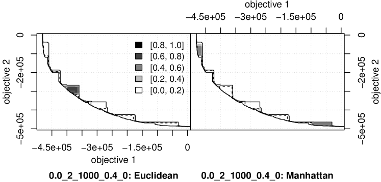
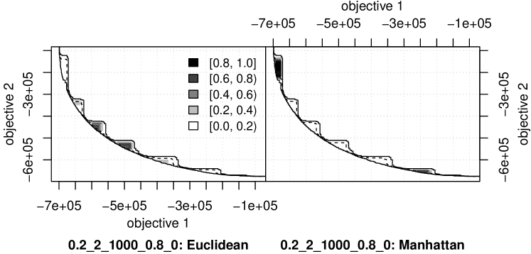
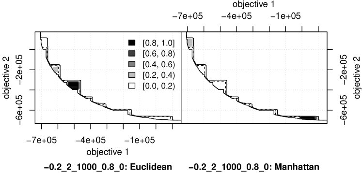
Figure 1: Comparing proposed Adaptive-Averages-Euclidean and Adaptive-Averages-Manhattan.

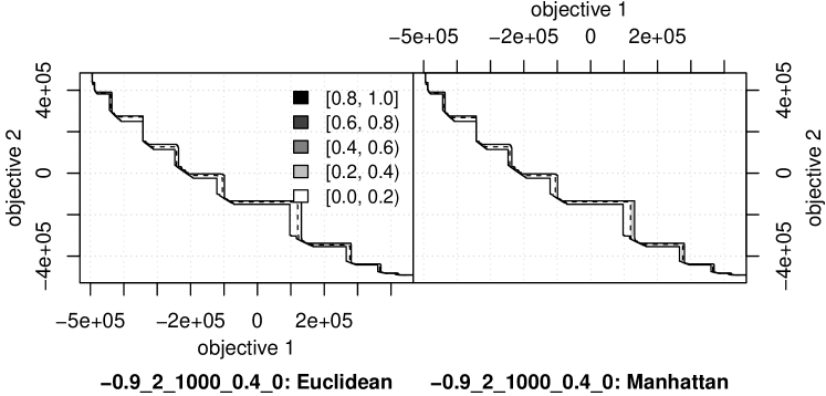
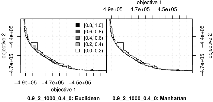
Figure 2: Comparing proposed Adaptive-Averages-Euclidean and Adaptive-Averages-Manhattan.

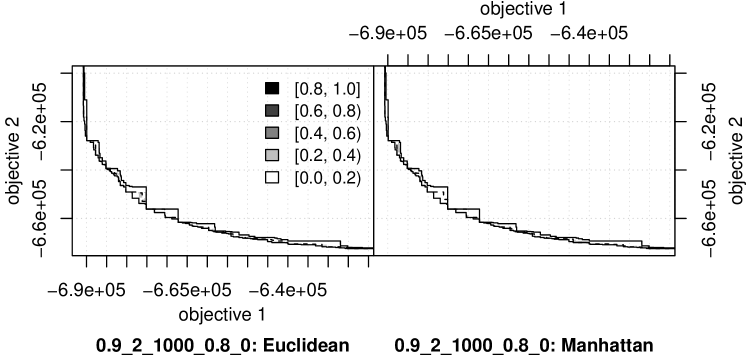
Figure 3: Comparing proposed Adaptive-Averages-Euclidean and Adaptive-Averages-Manhattan.

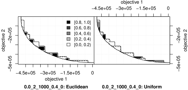
Figure 4: Comparing proposed Adaptive-Averages-Euclidean and Adaptive-Averages-Manhattan.

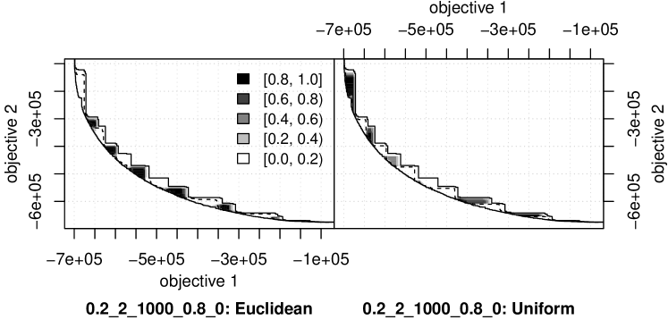
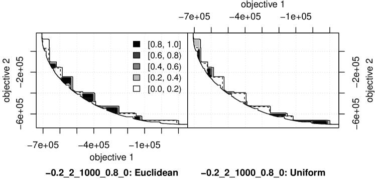
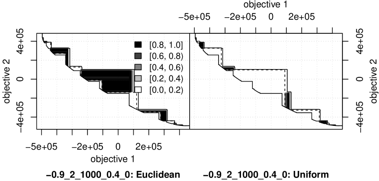
Figure 5: Comparing proposed Adaptive-Averages-Euclidean and Adaptive-Averages-Manhattan.

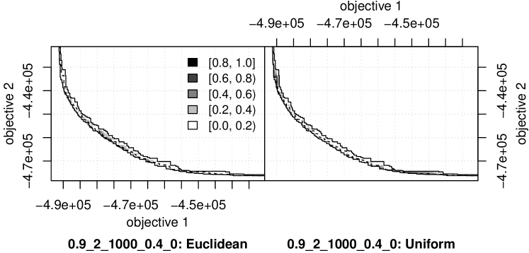
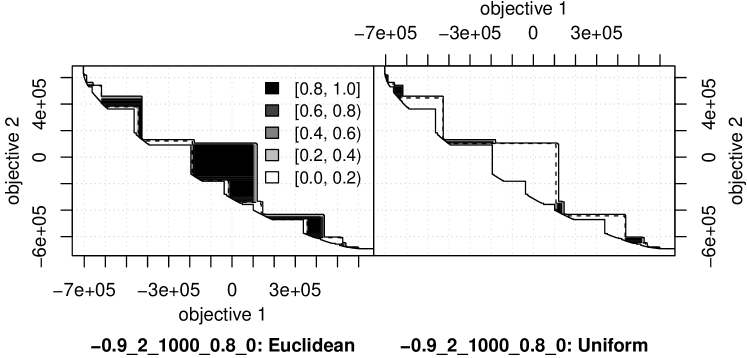
Figure 6: Comparing proposed Adaptive-Averages-Euclidean and Adaptive-Averages-Manhattan.

4.3 Performance Measures

4.3.1 Empirical Attainment Function (EAF)

The EAF of an algorithm gives the probability, estimated from multiple runs, that the non-dominated set produced by a single run of the algorithm dominates a particular point in the objective space. The visualisation of the EAF (Grunert da Fonseca et al., 2001) has been shown as a suitable graphical interpretation of the quality of the outcomes returned by local search methods. The visualisation of the differences between the EAFs of two alternative algorithms indicates how much better one method is compared to another in a particular region of the objective space (López-Ibáñez et al., 2010). EAF visualisations were generated using the eaf R package.

4.3.2 Hypervolume

The hypervolume (Zitzler and Thiele, 1998) is one of the most frequently used quality metrics in multi-objective optimisation because it never contradicts Pareto optimality and measures both the quality and diversity of a non-dominated set. The hypervolume measures the size of the objective space (the area in 2D, the volume in 3D) that is dominated by at least one of the points of a non-dominated set bounded by a reference point that is dominated by all points in all non-dominated sets under comparison, for a given problem. Larger hypervolume values indicate better performance. The reference points used for hypervolume calculation in this study are presented in Table 2. These values were derived experimentally: they are the highest values attained by the DA for each objective when using the uniform method of generating weights.

4.3.3 Number of Non-dominated Solutions

Although the number of non-dominated solutions found by a multi-objective algorithm is not sufficient to assess its performance, it can provide valuable information when compared with other quality metrics such as hypervolume. In this study, we report both the number of non-dominated solutions and the hypervolume achieved by each method.

5 Results and Discussion

The mean and standard deviation of hypervolume values of solutions found across 20 runs are presented in Table 3. Column Uniform presents the performance of the DA based on evenly generated weights (Algorithm 1), column Adaptive-Averages-Manhattan presents the performance of the DA based on an adaptive method (averages) of generating weights (Algorithm 3) where the distance metric is based on the Manhattan distance, column Adaptive-Averages-Euclidean presents the performance of the DA based on an adaptive method (averages) of generating weights (Algorithm 3) where the distance metric is based on the Euclidean distance and column Adaptive-Dichotomic-Euclidean presents the performance of the DA based on an adaptive method (dichotomic search) of generating weights (Algorithm 2) where the distance metric is based on the Euclidean distance.

For the problem instances with two objectives, executing the DA with the Uniform method leads to the worst performance on instances with negative or no correlation between their objectives. The Uniform method however leads to more promising performance on instances with positive correlations between their objectives. The DA reaches the best mean hypervolume when executed with the Uniform method on an instance with a positive correlation between its objectives ($0.9\_2\_1000\_0.8\_0$) and the same mean hypervolume as the DA executed with Adaptive-Averages-Euclidean or Adaptive-Dichotomic-Euclidean method on two instances with positive correlations between their objectives ($0.2\_2\_1000\_0.8\_0$ and $0.9\_2\_1000\_0.4\_0$). We show that running the DA with the Adaptive-Dichotomic-Euclidean method is consistently among the best on 6 of 7 mUBQP instances with 2 objectives. This method however cannot be applied to instances with more than 2 objectives. With the exception of instance ‘0.9_2_1000_0.8_0’, the proposed Adaptive-Averages-Euclidean is also consistently as good as or better than Uniform on instances with 2 objectives. We also show that the hypervolume of the DA with the proposed Adaptive-Averages-Euclidean is consistently either as good as or better than the existing counterpart Adaptive-Averages-Manhattan.

We show this performance difference in more detail using EAF visualisations in Figures 1–3. Darker regions indicate regions of the front where one algorithm is better than the other. We see more evenly distributed darker regions when the DA is executed with Adaptive-Averages-Euclidean compared to Adaptive-Averages-Manhattan. We also see more evenly distributed darker regions when the DA is executed with Adaptive-Averages-Euclidean compared to Uniform, as shown in the EAF plots in Figure 4–6) particularly on instances where higher mean hypervolume values were recorded.

For problems with 3 or 4 objectives, we do not present results for Adaptive-Dichotomic-Euclidean because it cannot be applied to problems with more than 2 objectives. When the DA is executed with the proposed Adaptive-Averages-Euclidean, significantly higher mean hypervolume values are attained when compared to Adaptive-Averages-Manhattan or Uniform on all mUBQP instances with 3 or 4 objectives. Uniform particularly presents the worst performance on all mUBQP instances with 3 or 4 objectives.

Table 4 also shows that Uniform returns the least mean number of non-dominated solutions. There is however no one adaptive method which consistently leads within the context of the number of non-dominated solutions found.

The better performance (hypervolume) of Adaptive-Averages-Euclidean compared to Adaptive-Averages-Euclidean indicates that Euclidean distance works better than Manhattan distance on the instances used in this work. The poorer performance of Uniform is not unexpected. It should be noted that in real-world scenarios, it is often the case that we do not want any of the objectives to have their weight equal to zero as this completely disregards the objective. In the case of uniform weights generated using the simplex lattice design, a minimum of $H=m$ is needed at the very least to explore weights where none of the values is equal to 0. The number of weights when $H=m$ is $\textit{n\_weights}=\binom{2m-1}{m-1}$. This value can grow very large as the number of objectives increases; 3 weights for 2 objectives, 10 weights for 3 objectives, 35 weights for 4 objectives, …, and 378 weights for 10 objectives. However, the adaptive approach explores a set of weights where none of the values is equal to 0 in a minimum of $m+1$ weights. Adaptive methods will therefore, particularly in scenarios where trying scalarisation weights greater than $\binom{2m-1}{m-1}$ is impractical, be more suitable.

6 Conclusions

This research explored various techniques for generating scalarisation weights within the context of multi-objective QUBO solving. The findings demonstrate that adaptive methods of weight generation can enhance the performance of the DA. We also show that the proposed method, which is based on Euclidean distance, leads to competitive performance on problems with 2 objectives and the best performance on instances with $3+$ objectives. Areas of further research include comparing the presented approaches on QUBO problems with more objectives, verifying whether increasing the number of weights leads to a difference in relative performance, and exploring multi-objective QUBO formulations of other combinatorial optimisation problems.

References

- Chang et al. [2000] T.-J. Chang, N. Meade, John E. Beasley, and Y. M. Sharaiha. Heuristics for cardinality constrained portfolio optimisation. Computers & Operations Research, 27(13):1271–1302, 2000.
- Hiroshi et al. [2021] Nakayama Hiroshi, Koyama Junpei, Yoneoka Noboru, and Miyazawa Toshiyuki. Third generation digital annealer technology, 2021. URL https://www.fujitsu.com/jp/documents/digitalannealer/researcharticles/DA_WP_EN_20210922.pdf.
- McGeoch and Farré [2020] Catherine C. McGeoch and Pau Farré. The D-Wave advantage system: An overview. Technical report, D-Wave Systems Inc., Burnaby, BC, Canada, 2020. URL https://www.dwavesys.com/media/s3qbjp3s/14-1049a-a_the_d-wave_advantage_system_an_overview.pdf.
- Elsokkary et al. [2017] Nada Elsokkary, Faisal Shah Khan, Davide La Torre, Travis S. Humble, and Joel Gottlieb. Financial portfolio management using D-Wave’s quantum optimizer: The case of Abu Dhabi securities exchange. Technical report, Oak Ridge National Lab, Oak Ridge, TN, USA, 2017. URL https://www.osti.gov/biblio/1423041.
- Phillipson and Bhatia [2021] Frank Phillipson and Harshil Singh Bhatia. Portfolio optimisation using the D-Wave quantum annealer. In Maciej Paszynski, Dieter Kranzlmüller, Valeria V. Krzhizhanovskaya, Jack J. Dongarra, and Peter M. A. Sloot, editors, Computational Science – ICCS 2021, pages 45–59. Springer International Publishing, Cham, Switzerland, 2021.
- Martins et al. [2021] Ricardo Martins, Nuno Lourenço, Ricardo Póvoa, and Nuno Horta. Shortening the gap between pre-and post-layout analog ic performance by reducing the lde-induced variations with multi-objective simulated quantum annealing. Engineering Applications of Artificial Intelligence, 98:104102, 2021.
- Ayodele et al. [2022] Mayowa Ayodele, Richard Allmendinger, Manuel López-Ibáñez, and Matthieu Parizy. A study of scalarisation techniques for multi-objective QUBO solving. Arxiv preprint arXiv:2210.11321, 2022. doi:10.48550/arXiv.2210.11321.
- Zitzler and Thiele [1998] Eckart Zitzler and Lothar Thiele. Multiobjective optimization using evolutionary algorithms - A comparative case study. In Agoston E. Eiben, Thomas Bäck, Marc Schoenauer, and Hans-Paul Schwefel, editors, Parallel Problem Solving from Nature – PPSN V, volume 1498 of Lecture Notes in Computer Science, pages 292–301, Heidelberg, 1998. Springer. doi:10.1007/BFb0056872.
- Dubois-Lacoste et al. [2011] Jérémie Dubois-Lacoste, Manuel López-Ibáñez, and Thomas Stützle. Improving the anytime behavior of two-phase local search. Annals of Mathematics and Artificial Intelligence, 61(2):125–154, 2011. doi:10.1007/s10472-011-9235-0.
- Liefooghe et al. [2015] Arnaud Liefooghe, Sébastien Verel, Luís Paquete, and Jin-Kao Hao. Experiments on local search for bi-objective unconstrained binary quadratic programming. In António Gaspar-Cunha, Carlos Henggeler Antunes, and Carlos A. Coello Coello, editors, Evolutionary Multi-criterion Optimization, EMO 2015 Part I, volume 9018 of Lecture Notes in Computer Science, pages 171–186. Springer, Heidelberg, 2015.
- Steuer [1986] R. E. Steuer. Multiple Criteria Optimization: Theory, Computation and Application. Wiley Series in Probability and Mathematical Statistics. John Wiley & Sons, New York, NY, 1986.
- Liefooghe et al. [2014] Arnaud Liefooghe, Sébastien Verel, and Jin-Kao Hao. A hybrid metaheuristic for multiobjective unconstrained binary quadratic programming. Applied Soft Computing, 16:10–19, 2014.
- Matsubara et al. [2020] Satoshi Matsubara, Motomu Takatsu, Toshiyuki Miyazawa, Takayuki Shibasaki, Yasuhiro Watanabe, Kazuya Takemoto, and Hirotaka Tamura. Digital annealer for high-speed solving of combinatorial optimization problems and its applications. In 2020 25th Asia and South Pacific Design Automation Conference (ASP-DAC), pages 667–672. IEEE, 2020. doi:10.1109/ASP-DAC47756.2020.9045100.
- Zhou et al. [2018] Ying Zhou, Jiahai Wang, Ziyan Wu, and Keke Wu. A multi-objective tabu search algorithm based on decomposition for multi-objective unconstrained binary quadratic programming problem. Knowledge-Based Systems, 141:18–30, 2018.
- Chen et al. [2022] Xin Chen, Jiacheng Yin, Dongjin Yu, and Xulin Fan. A decomposition-based many-objective evolutionary algorithm with adaptive weight vector strategy. Applied Soft Computing, 128:109412, 2022. ISSN 1568-4946. URL https://www.sciencedirect.com/science/article/pii/S1568494622005476.
- Zhang and Li [2007] Qingfu Zhang and Hui Li. Moea/d: A multiobjective evolutionary algorithm based on decomposition. IEEE Transactions on evolutionary computation, 11(6):712–731, 2007.
- Grunert da Fonseca et al. [2001] Viviane Grunert da Fonseca, Carlos M. Fonseca, and Andreia O. Hall. Inferential performance assessment of stochastic optimisers and the attainment function. In Eckart Zitzler, Kalyanmoy Deb, Lothar Thiele, Carlos A. Coello Coello, and David Corne, editors, Evolutionary Multi-criterion Optimization, EMO 2001, volume 1993 of Lecture Notes in Computer Science, pages 213–225. Springer, Heidelberg, 2001. doi:10.1007/3-540-44719-9_15.
- López-Ibáñez et al. [2010] Manuel López-Ibáñez, Luís Paquete, and Thomas Stützle. Exploratory analysis of stochastic local search algorithms in biobjective optimization. In Thomas Bartz-Beielstein, Marco Chiarandini, Luís Paquete, and Mike Preuss, editors, Experimental Methods for the Analysis of Optimization Algorithms, pages 209–222. Springer, Berlin, Germany, 2010. doi:10.1007/978-3-642-02538-9_9.