Quantum channel decomposition with pre- and post-selection

Abstract

The quantum channel decomposition techniques, which contain the so-called probabilistic error cancellation and gate/wire cutting, are powerful approach for simulating a hard-to-implement (or an ideal) unitary operation by concurrently executing relatively easy-to-implement (or noisy) quantum channels. However, such virtual simulation necessitates an exponentially large number of decompositions, thereby significantly limiting their practical applicability. This paper proposes a channel decomposition method for target unitaries that have their input and output conditioned on specific quantum states, namely unitaries with pre- and post-selection. Specifically, we explicitly determine the requisite number of decomposing channels, which could be significantly smaller than the selection-free scenario. Furthermore, we elucidate the structure of the resulting decomposed unitary. We demonstrate an application of this approach to the quantum linear solver algorithm, highlighting the efficacy of the proposed method.

I Introduction

Running a large quantum circuit is a challenging task, unless the ideal quantum error correction would be incorporated. To simulate such circuit without error correction or to relax the strict condition for realizing error correction, several techniques have been developed – the quantum channel decomposition is one such effective method for this purpose.

The idea of channel decomposition is, as the name implies, to decompose a hard-to-implement (or an ideal) quantum channel to the sum of relatively easy-to-implement (or realistic) channels. The so-called probabilistic error cancellation [1, 2, 3, 4] can be formulated in this framework. Also, especially when the target channel is an ideal unitary operator and the decomposing channels are given by products of smaller unitaries, then the method is called the gate cutting [5, 6, 7, 8, 9, 10, 11]. In addition, when the target gate is a set of identity operators along the lines of a quantum circuit diagram, it is called the wire cutting [12, 13, 14, 15, 16, 17, 18, 19, 10, 20, 21, 22, 23, 24, 25]. However, these channel decomposition methods have the common issue of exponential computational overhead; that is, the number of decomposing channel grows exponentially with respect to the number of qubits of the target channel.

In this paper, we propose a general channel decomposition method that reduces the number of decomposition, though the exponential scaling is kept. The idea is to pre- and post-select the states for a target unitary gate. More precisely, the input state to the target unitary gate and the output state from the target are both limited to certain type of quantum states living in subspaces of the entire Hilbert space. This situation is often found in several quantum algorithms. Actually, when the target is a unitary operator representing the entire circuit, the initial state is usually fixed (typically, to the product of $\ket{0}$); also, when the target unitary gate corresponds to a sub-circuit of the entire circuit, the input state to that unitary can still be restricted, as in the case of Grover search algorithm [26]. Also, the output state is confined to a subspace in some quantum algorithms, such as probabilistic state preparation algorithms that succeed only when a part of the output state is projected to a certain fixed state by measurement; this idea is applicable to both cases where the target unitary gate is an entire circuit and a part of the entire circuit. Under this pre- and post-selection condition, we explicitly identify the necessary number of decomposing channels (Theorem 1) and moreover the structure of the resulting decomposed unitary gate (Theorem 2). Then, we demonstrate the proposed method with a 5-qubits quantum linear solver algorithm (Harrow-Hassidim-Lloyd, HHL algorithm) [27]; notably, while the original circuit is of 212 depth and contains 108 CNOT gates, it can be decomposed to only three circuits that are composed of the product of one-qubit gates and thus much easier to implement than the original.

II Preliminaries

II.1 Quantum channel decomposition

We consider the following $n$-qubit quantum channel:

$$\rho\mapsto\rho^{\prime}=U^{(n)}\rho\,U^{(n){\dagger}}\,.$$ (1)

Here $U^{(n)}$ is an $N\times N$ unitary matrix, where $N=2^{n}$. Also, $\rho$ and $\rho^{\prime}$ denote the density matrix of the $n$-qubit system before and after the unitary gate operation, respectively. For later convenience, we define the linear map $[U]$ as

$$[U]\rho:=U\rho\,U^{\dagger}\,.$$ (2)

Using this symbol, we can express Eq. (1) as

$$\rho^{\prime}=[U^{(n)}]\rho\,.$$ (3)

One can decompose $[U^{(n)}]$ into a set of the linearly independent completely positive and trace-nonincreasing maps [2, 6, 7, 3] $\{[V^{(n)}_{i}]\}$ as

$$[U^{(n)}]\,=\,\sum_{i=1}^{D}c_{i}\,[V^{(n)}_{i}]\,,$$ (4)

where the coefficients $\{c_{i}\}$ are real. $\{[V^{(n)}_{i}]\}$ is the set of the quantum channels which are easier to implement than $[U^{(n)}]$. We will specify $\{[V^{(n)}_{i}]\}$ later. The number of the independent maps, $D$, should be larger than $N^{4}=16^{n}$ to satisfy the equality in Eq. (4) for a general $[U^{(n)}]$. The coefficients $\{c_{i}\}$ are uniquely determined when $D=16^{n}$, while they are ambiguously determined when $D>16^{n}$. We call the decomposition (4) the “quantum channel decomposition” .

The motivation to conduct the channel decomposition (4) arises when $[U^{(n)}]$ is more difficult to implement than $\{[V^{(n)}_{i}]\}$. Actually, Eq. (4) implies that we can simulate the output of the harder quantum channel $[U^{(n)}]$ by combining the output of the easier quantum channels $\{[V^{(n)}_{i}]\}$. In particular, the Monte-Carlo method can be applied to calculate the expectation of an observable $B$ for the output state $\rho^{\prime}$ via

$${\rm Tr}\left(B[U^{(n)}]\rho\right)=\gamma\sum_{i=1}^{D}\frac{|c_{i}|}{\gamma}\,{\rm sign}(c_{i})\,{\rm Tr}\left(B[V_{i}^{(n)}]\rho\right),$$ (5)

where $\gamma=\sum_{i=1}^{D}|c_{i}|$. That is, by sampling $\{[V^{(n)}_{i}]\}$ with probability $|c_{i}|/\gamma$ followed by calculating the expectation of $B$, the hard calculation of the expectation of $B$ becomes doable. The overhead for this simulation is quantified by $\gamma$, because the approximation error of the expectation is $\mathcal{O}(\gamma/\sqrt{N_{\rm{s}}})$ with $N_{\rm{s}}$ being the total number of sampling. Hence, we call $\gamma$ the sampling overhead.

II.2 Gate decomposition

The goal of gate decomposition is to decompose the quantum channel $[U^{(n)}]$ into a set of quantum channels consisting of only local quantum operations as follows:

$$[U^{(n)}]\,=\,\sum_{i=1}^{D}c_{i}\,[V^{(1)}_{i_{1}}\otimes V^{(1)}_{i_{2}}\otimes\cdots\otimes V^{(1)}_{i_{n}}]\,,$$ (6)

where $i_{k}$ runs from $1$ to $D_{k}\,(\geq 16)$ and $i$ runs in the form $i=\sum_{k=1}^{n}(\prod_{k^{\prime}=1}^{k}D_{k^{\prime}-1})i_{k}$ with $D_{0}=1$. $D$ is given as $D=D_{1}D_{2}\cdots D_{n}$. $\{V^{(1)}_{i_{a}}\,(a=1,2,\cdots,n)\}$ denotes a set of one-qubit operations. The one-qubit operations consist of not only one-qubit unitary gate but also non-unitary operations such as measurement operations.

Note that the basis $\{V^{(1)}_{i_{a}}\}$ is not unique. Also, the coefficients $\{c_{i}\}$ depend on the basis. In this paper, we employ the basis introduced in Ref. [2] which is listed in Table 1. Other bases are considered by Refs. [6, 7, 3], for examples.

Table 1: 16 linearly independent operations for the one-qubit gate decomposition. $I$ denotes $2\times 2$ identity matrix. $X$, $Y$ and $Z$ are Pauli matrices. This set of operators was introduced in Ref. [2].

$[{V}^{(1)}_{1}]$	$[{I}]$
$[{V}^{(1)}_{2}]$	$[{X}]$
$[{V}^{(1)}_{3}]$	$[{Y}]$
$[{V}^{(1)}_{4}]$	$[{Z}]$
$[{V}^{(1)}_{5}]$	$[{R}_{X}]=[(1/\sqrt{2})({I}+i{X})]$
$[{V}^{(1)}_{6}]$	$[{R}_{Y}]=[(1/\sqrt{2})({I}+i{Y})]$
$[{V}^{(1)}_{7}]$	$[{R}_{Z}]=[(1/\sqrt{2})({I}+i{Z})]$
$[{V}^{(1)}_{8}]$	$[{R}_{YZ}]=[(1/\sqrt{2})({Y}+{Z})]$
$[{V}^{(1)}_{9}]$	$[{R}_{ZX}]=[(1/\sqrt{2})({Z}+{X})]$
$[{V}^{(1)}_{10}]$	$[{R}_{XY}]=[(1/\sqrt{2})({X}+{Y})]$
$[{V}^{(1)}_{11}]$	$[{\pi}_{X}]=[(1/2)({I}+{X})]$
$[{V}^{(1)}_{12}]$	$[{\pi}_{Y}]=[(1/2)({I}+{Y})]$
$[{V}^{(1)}_{13}]$	$[{\pi}_{Z}]=[(1/2)({I}+{Z})]$
$[{V}^{(1)}_{14}]$	$[{\pi}_{YZ}]=[(1/2)({Y}+i{Z})]$
$[{V}^{(1)}_{15}]$	$[{\pi}_{ZX}]=[(1/2)({Z}+i{X})]$
$[{V}^{(1)}_{16}]$	$[{\pi}_{XY}]=[(1/2)({X}+i{Y})]$

Once the basis is fixed, we can determine the coefficients $\{c_{i}\}$ by solving Eq. (6) for a given $U^{(n)}$. Here we present some results of the gate decomposition of specific targets as examples. We consider controlled-NOT (CNOT), Toffoli, and three-qubit Quantum Fourier Transformation (QFT₃) gates as the target unitary channel. In the computational basis, these unitary matrices are represented by

$$\mbox{CNOT}:\quad U^{(n)} \,=\,\begin{pmatrix}1&0&0&0\\ 0&1&0&0\\ 0&0&0&1\\ 0&0&1&0\end{pmatrix}\,,$$ (7)

$$\mbox{Toffoli}:\quad U^{(n)} \,=\,\begin{pmatrix}1&0&0&0&0&0&0&0\\ 0&1&0&0&0&0&0&0\\ 0&0&1&0&0&0&0&0\\ 0&0&0&1&0&0&0&0\\ 0&0&0&0&1&0&0&0\\ 0&0&0&0&0&1&0&0\\ 0&0&0&0&0&0&0&1\\ 0&0&0&0&0&0&1&0\end{pmatrix}\,,$$ (8)

$$\mbox{QFT}_{3}:\quad U^{(n)} \,=\,\frac{1}{\sqrt{8}}\begin{pmatrix}1&1&1&1&1&1&1&1\\ 1&\omega&\omega^{2}&\omega^{3}&\omega^{4}&\omega^{5}&\omega^{6}&\omega^{7}\\ 1&\omega^{2}&\omega^{4}&\omega^{6}&1&\omega^{2}&\omega^{4}&\omega^{6}\\ 1&\omega^{3}&\omega^{6}&\omega&\omega^{4}&\omega^{7}&\omega^{2}&\omega^{5}\\ 1&\omega^{4}&1&\omega^{4}&1&\omega^{4}&1&\omega^{4}\\ 1&\omega^{5}&\omega^{2}&\omega^{7}&\omega^{4}&\omega^{1}&\omega^{6}&\omega^{3}\\ 1&\omega^{6}&\omega^{4}&\omega^{2}&1&\omega^{6}&\omega^{4}&\omega^{2}\\ 1&\omega^{7}&\omega^{6}&\omega^{5}&\omega^{4}&\omega^{3}&\omega^{2}&\omega\end{pmatrix}\,,$$ (9)

with $\omega=e^{i\pi/4}$. The sampling overheads $\gamma$ for the gate decomposition of these unitary channels $[U^{(n)}]$ are obtained as

$$\mbox{CNOT}:\quad \gamma=\sum_{i=1}^{16^{2}}|c_{i}|=9\,,$$ (10)

$$\mbox{Toffoli}:\quad \gamma=\sum_{i=1}^{16^{3}}|c_{i}|=37\,,$$ (11)

$$\mbox{QFT}_{3}:\quad \gamma=\sum_{i=1}^{16^{3}}|c_{i}|\simeq 261\,.$$ (12)

The explicit expressions of the gate decomposition for the above examples are summarized in Appendix A.

III Main results

III.1 Notation

Let $A$ be an $m\times n$ matrix. We define the vectorization of $A$, denoted by $|A\,\rangle\rangle$, as the $(mn\times 1)$-vector with the columns of the matrix $A$ stacked on top of each other [28]. We also define $\langle\langle\,A|$ as $\langle\langle\,A|=(|A\,\rangle\rangle)^{\dagger}$. The inner product $\langle\langle\,A|B\,\rangle\rangle$ is calculated as $\langle\langle\,A|B\,\rangle\rangle=\mbox{Tr}[A^{\dagger}B]$. We have

$$|ABC\,\rangle\rangle\,=\,(C^{T}\otimes A)|B\,\rangle\rangle\,.$$ (13)

for arbitrary matrices $A$, $B$ and $C$ [28]. We will use this equation later.

Given an $n$-qubit quantum channel $\mathcal{A}$, we introduce the Choi-matrix $\mbox{C}(\mathcal{A})$ as

$$\mbox{C}(\mathcal{A})\,=\,\sum_{i=1}^{N}\sum_{j=1}^{N}E_{ij}\otimes\mathcal{A}(E_{ij})\,,$$ (14)

where $N=2^{n}$ and $E_{ij}=\ket{i}\!\!\bra{j}$ in the computational basis. In particular, for the quantum channel $\mathcal{A}(\rho)=\sum_{i=1}^{a}c_{i}[V^{(n)}_{i}]\rho$, we have

$$\mbox{C}(\mathcal{A})=\sum_{i=1}^{a}c_{i}|V^{(n)}_{i}\,\rangle\rangle~{}\langle\langle\,V^{(n)}_{i}|\,.$$ (15)

It is known that the mapping $\mathcal{A}\mapsto\mbox{C}(\mathcal{A})$ is isomorphism and affine (Jamiolkowski–Choi isomorphism) [29, 30, 31, 32].

III.2 Quantum channel with pre- and post-selection

We consider the $n$-qubit quantum channel $[U^{(n)}]$ given in Eq. (3), where the input state $\rho$ and the output state $\rho^{\prime}$ are specified somehow. In particular, we are often interested in the situation where these states are restricted in some subspaces; such input and output states, $\rho_{\mathrm{in}}$ and $\rho_{\mathrm{out}}$, can be expressed as

$$\rho_{\mathrm{in}}\,=\,\frac{P_{\mathrm{in}}\rho P_{\mathrm{in}}}{\mbox{Tr}(\rho P_{\mathrm{in}})}\,,\quad\rho_{\mathrm{out}}\,=\,\frac{P_{\mathrm{out}}\rho^{\prime}P_{\mathrm{out}}}{\mbox{Tr}(\rho^{\prime}P_{\mathrm{out}})}\,.$$ (16)

Here, $P_{\mathrm{in}}$ and $P_{\mathrm{out}}$ are the projection matrices (Recall ${P^{\dagger}_{\mathrm{in,out}}=P_{\mathrm{in,out}}}$ and $P^{2}_{\mathrm{in,out}}=P_{\mathrm{in,out}}$) which respectively describe the pre- and post-selection of the quantum states. We note that $\max(r_{\mathrm{in}},r_{\mathrm{out}})\leq N=2^{n}$ where

$$r_{\mathrm{in}}:={\mathrm{rank}}P_{\mathrm{in}}\,,\quad r_{\mathrm{out}}:={\mathrm{rank}}P_{\mathrm{out}}\,.$$ (17)

The quantum channel with the post- and pre-selection is described as

$$[P_{\mathrm{out}}U^{(n)}P_{\mathrm{in}}]\,,$$ (18)

up to the normalization factor $\mbox{Tr}(\rho P_{\mathrm{in}})$ and $\mbox{Tr}(\rho^{\prime}P_{\mathrm{out}})$. Now, $[P_{\mathrm{out}}U^{(n)}P_{\mathrm{in}}]$ can be decomposed with fewer bases than the case we decompose $[U^{(n)}]$. The reason is as follows. The map $[P_{\mathrm{out}}U^{(n)}P_{\mathrm{in}}]$ except for the parts determined by the projection operators is described by the linear map from the quantum states on $r_{\mathrm{in}}$-dimensional Hilbert space to those on $r_{\mathrm{out}}$-dimensional Hilbert space. This means that the quantum channel with post- and pre-selection $[P_{\mathrm{out}}U^{(n)}P_{\mathrm{in}}]$ is inherently described by $r^{2}_{\mathrm{in}}\times r^{2}_{\mathrm{out}}$ matrix. The size of the matrix representation of $[P_{\mathrm{out}}U^{(n)}P_{\mathrm{in}}]$ is therefore smaller than that of the matrix representation of $[U^{(n)}]$, $N^{4}=16^{n}$.

To be more concrete, let us discuss the structure of $[P_{\rm{out}}U^{(n)}P_{\rm{in}}]$ explicitly. The Choi-matrix of the quantum channel with pre- and post-selection (18) is given as

$$\mbox{C}([P_{\mathrm{out}}U^{(n)}P_{\mathrm{in}}])\,=\,{\bf{P}}\mbox{C}([U^{(n)}]){\bf{P}}\,,$$ (19)

where ${\bf{P}}\,=\,P_{\mathrm{in}}\otimes P_{\mathrm{out}}$. Here we used Eqs. (13) and (15). The matrix structure of the right-handed side of Eq. (19) can be more clarified by diagonalizing the projection matrices as

$$P_{\mathrm{in}} \,=\,O^{\dagger}_{\mathrm{in}}P_{d,\mathrm{in}}O_{\mathrm{in}}\,,\quad P_{d,\mathrm{in}}\,=\,\begin{pmatrix}I_{r_{\mathrm{in}}}&\phantom{I_{a}}\\ \phantom{I_{a}}&\phantom{I_{a}}\end{pmatrix}\,,$$ (20)

$$P_{\mathrm{out}} \,=\,O_{\mathrm{out}}P_{d,\mathrm{out}}O^{\dagger}_{\mathrm{out}}\,,\quad P_{d,\mathrm{out}}\,=\,\begin{pmatrix}I_{r_{\mathrm{out}}}&\phantom{I_{a}}\\ \phantom{I_{a}}&\phantom{I_{a}}\end{pmatrix}\,,$$ (21)

where $I_{m}$ denotes the $m\times m$ identity matrix. The components of the blank part are zero. $O_{\mathrm{in}}$ and $O_{\mathrm{out}}$ are known $N\times N$ unitary matrices that are determined to satisfy Eqs. (20) and (21), respectively. We here employ the computational basis for the above matrix representations just for simplicity.

We comment on the implementation of the diagonalization unitary matrices, $O_{\mathrm{in}}$ and $O_{\mathrm{out}}$, on a circuit. When the projection operator can be written as $P=\ket{\psi}\!\!\bra{\psi}$ with $\ket{\psi}$ being a pure state, the unitary matrix can be implemented as the corresponding state preparation operator. In addition, by applying the purification technique, we can implement the unitary operator as a state preparation process, for the general case where $P$ has a form of mixed state, i.e., a linear combination of the pure projection operators.

Plugging Eqs. (20) and (21) into Eq. (19) and using Eq. (13), we obtain

$$\mbox{C}([P_{\mathrm{out}}U^{(n)}P_{\mathrm{in}}]) \,=\,{\bf{O}}^{\dagger}{\bf{P}}_{d}\mbox{C}([O_{\mathrm{out}}U^{(n)}O_{\mathrm{in}}]){\bf{P}}_{d}{\bf{O}}\,,$$ (22)

where ${\bf{O}}=O_{\mathrm{in}}\otimes O^{\dagger}_{\mathrm{out}}$ and

$${\bf{P}}_{d}=P_{d,\mathrm{in}}\otimes P_{d,\mathrm{out}}\,.$$ (23)

It should be noted that ${\bf{P}}_{d}\mbox{C}([O_{\mathrm{out}}U^{(n)}O_{\mathrm{in}}]){\bf{P}}_{d}$ is the principal submatrix of $\mbox{C}([O_{\mathrm{out}}U^{(n)}O_{\mathrm{in}}])$. The submatrix can be represented as

$${\bf{P}}_{d}\mbox{C}([O_{\mathrm{out}}U^{(n)}O_{\mathrm{in}}]){\bf{P}}_{d}\,=\,|V^{(n)}\,\rangle\rangle~{}\langle\langle\,V^{(n)}|\,,$$ (24)

where $V^{(n)}$ is the $N\times N$ matrix of the form

$$V^{(n)}\,=\,\begin{pmatrix}V&\phantom{V}\\ \phantom{V}&\phantom{V}\end{pmatrix}.$$ (25)

Here, $V$ is the $r_{\mathrm{out}}\times r_{\mathrm{in}}$ matrix given by

$$V\,=\,\begin{pmatrix}(v_{1})_{1}&\cdots&(v_{1})_{r_{\mathrm{in}}}\\ \vdots&\ddots&\vdots\\ (v_{r_{\mathrm{out}}})_{1}&\cdots&(v_{r_{\mathrm{out}}})_{r_{\mathrm{in}}}\\ \end{pmatrix}$$ (26)

with

$$(v_{i})_{j} \,=\,\langle\langle\,E_{ji}|O_{\mathrm{out}}U^{(n)}O_{\mathrm{in}}\,\rangle\rangle$$

$$\,=\,\langle\langle\,O^{\dagger}_{\mathrm{out}}E_{ji}O^{\dagger}_{\mathrm{in}}|U^{(n)}\,\rangle\rangle\,.$$ (27)

Combining Eqs. (22) and (24), we finally arrive at $\mbox{C}([P_{\mathrm{out}}U^{(n)}P_{\mathrm{in}}])\,=\,\mbox{C}([O_{\mathrm{out}}V^{(n)}O_{\mathrm{in}}])$ which results in

$$[P_{\mathrm{out}}U^{(n)}P_{\mathrm{in}}]\,=\,[O_{\mathrm{out}}V^{(n)}O_{\mathrm{in}}]\,.$$ (28)

It is now clear that the $U^{(n)}$-dependent part of $[P_{\mathrm{out}}U^{(n)}P_{\mathrm{in}}]$ is summarized into $V^{(n)}$ whose non-trivial components are collected in the $r_{\rm{out}}\times r_{\rm{in}}$ matrix $V$.

How can $V^{(n)}$ be implemented in a quantum circuit, then? We express $V^{(n)}$ givn in Eq. (25) as

$$V^{(n)}\,=\,\ket{0}\!\!\bra{0}^{\otimes(n-\tilde{n})}\otimes\widetilde{V}^{(\tilde{n})}$$ (29)

where

$$\tilde{n}\,=\,\lceil{\log_{2}{\mathrm{max}}(r_{\mathrm{in}},r_{\mathrm{out}})\rceil}\,.$$ (30)

Here we define the $2^{\tilde{n}}\times 2^{\tilde{n}}$ matrix $\widetilde{V}^{(\tilde{n})}$ with the $r_{\mathrm{out}}\times r_{\mathrm{in}}$ matrix $V$ embedded in the upper left component. The equation (29) implies that we can implement $V^{(n)}$ by the $n$-qubit circuit where the first $(n-\tilde{n})$ qubits are performed by measure-and-prepare operations independently, and the other qubits are acted on by $\widetilde{V}^{(\tilde{n})}$. We note that $\widetilde{V}^{(\tilde{n})}$ is not unitary in general. This means that we need measure-and-prepare operations to implement $\widetilde{V}^{(\tilde{n})}$. We will show an example of implementation in Section IV.

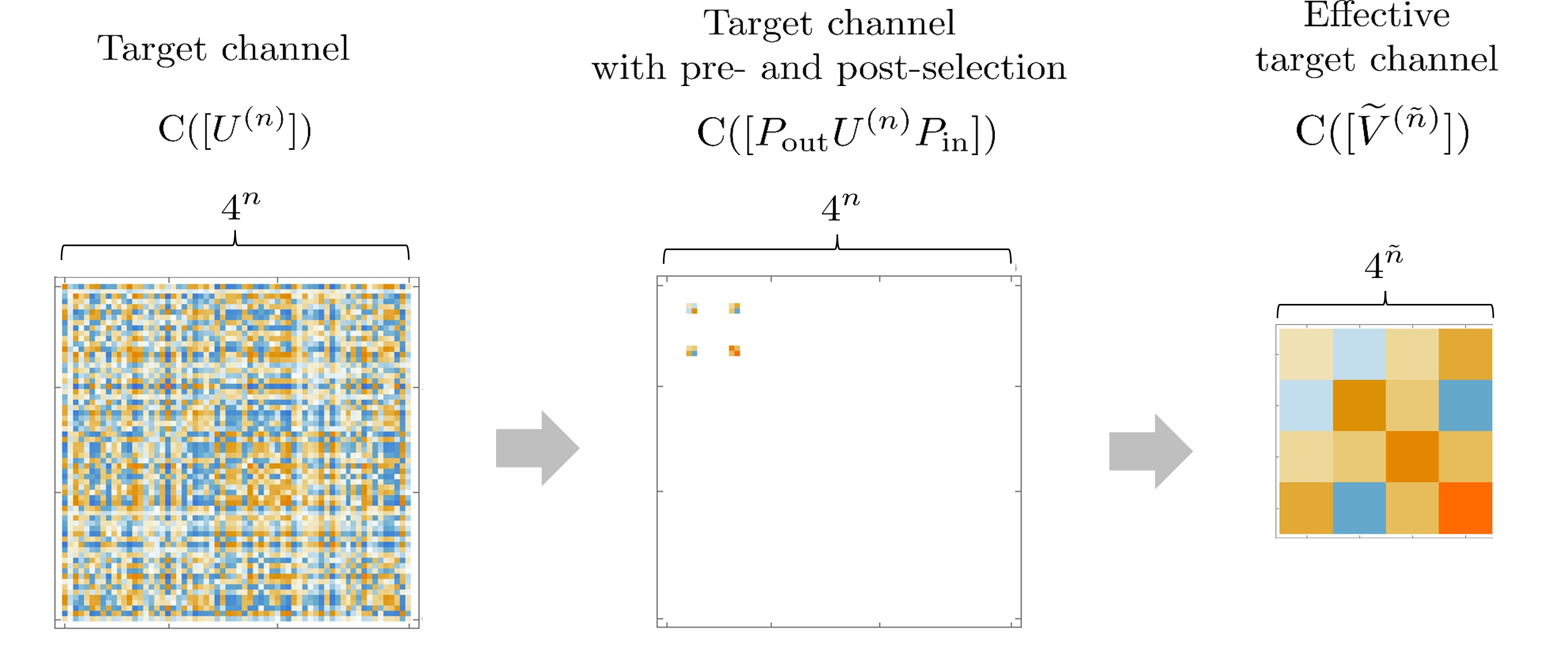
Figure 1: Relationship between the $n$-qubit channel with and without pre- and post-selection. We here consider the $n=3$ case where $P_{\rm{in}}=\ket{0}\!\!\bra{0}\otimes\ket{0}\!\!\bra{0}\otimes I$ and $P_{\rm{out}}=\ket{1}\!\!\bra{1}\otimes\ket{0}\!\!\bra{0}\otimes I$ as an example. The left, middle and right matrices respectively correspond to the Choi matrices of the target unitary without the projection operations $[U^{(n)}]$, the target with the projection operators $[P_{\rm{out}}U^{(n)}P_{\rm{in}}]$, and the effective target $[\widetilde{V}^{(\tilde{n})}]$.

Figure 1 shows the schematic picture of the relationship among $[U^{(n)}]$, $[P_{\rm{out}}U^{(n)}P_{\rm{in}}]$, and $[\widetilde{V}^{(\tilde{n})}]$. We here consider the $n=3$ case where $P_{\rm{in}}=\ket{0}\!\!\bra{0}\otimes\ket{0}\!\!\bra{0}\otimes I$ and $P_{\rm{out}}=\ket{1}\!\!\bra{1}\otimes\ket{0}\!\!\bra{0}\otimes I$ as an example. The left, middle and right matrices in Fig. 1 correspond to $\mbox{C}([U^{(n)}])$, $\mbox{C}([P_{\rm{out}}U^{(n)}P_{\rm{in}}])$, and $\mbox{C}([\widetilde{V}^{(\tilde{n})}])$, respectively. We observe that $\mbox{C}([P_{\rm{out}}U^{(n)}P_{\rm{in}}])$ is the principle submatrix of $\mbox{C}([U^{(n)}])$ where the subtraction is specified by $P_{\rm{in}}$ and $P_{\rm{out}}$. The number of non-trivial components of $\mbox{C}([P_{\rm{out}}U^{(n)}P_{\rm{in}}])$ corresponds to $r_{\rm{out}}\times r_{\rm{in}}$. $\mbox{C}([\widetilde{V}^{(\tilde{n})}])$ is constructed by gathering the non-trivial components of $\mbox{C}([P_{\rm{out}}U^{(n)}P_{\rm{in}}])$. It should be emphasized that the matrix size of $\mbox{C}([\widetilde{V}^{(\tilde{n})}])$ is much smaller than $\mbox{C}([{U}^{({n})}])$.

Combining Eq. (28) and (29), we arrive at the following theorem. A schematic picture of this fact is given in Fig. 2.

Theorem 1.

Let $P_{\mathrm{in}}$ and $P_{\mathrm{out}}$ be projection matrices with ${\mathrm{rank}}P_{\mathrm{in}}=r_{\mathrm{in}}$ and ${\mathrm{rank}}P_{\mathrm{in}}=r_{\mathrm{in}}$. Then, the $n$-qubit quantum channel with the pre- and post-selection, $[P_{\mathrm{out}}U^{(n)}P_{\mathrm{in}}]$, satisfies

$$[P_{\mathrm{out}}U^{(n)}P_{\mathrm{in}}]\,=\,[O_{\mathrm{out}}(\ket{0}\!\!\bra{0}^{\otimes(n-\tilde{n})}\otimes\widetilde{V}^{(\tilde{n})})O_{\mathrm{in}}]\,,$$ (31)

where $\tilde{n}=\lceil{\log_{2}{\mathrm{max}}(r_{\mathrm{in}},r_{\mathrm{out}})\rceil}$ and $\widetilde{V}^{(\tilde{n})}$ denotes $2^{\tilde{n}}\times 2^{\tilde{n}}$ matrix. $O_{\rm{in}}$ and $O_{\rm{out}}$ are known unitary matrices which diagonalize $P_{\rm{in}}$ and $P_{\rm{out}}$ as Eqs. (20) and (21). $\widetilde{V}^{(\tilde{n})}$ is obtained from Eqs. (25), (27) and (29).

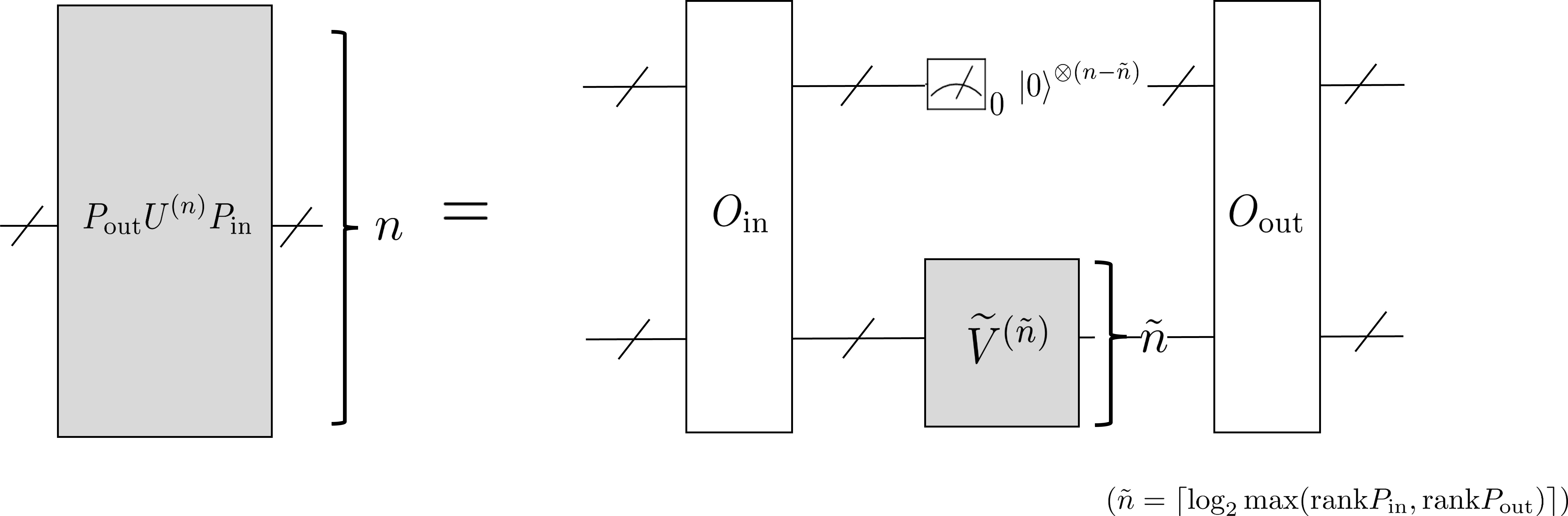
Figure 2: Schematic picture of theorem 1. The $n$-qubit quantum circuit with the pre- and post-selection (left) can be regarded as the quantum circuit shown in the right-handed side. $O_{\rm{in}}$ and $O_{\rm{out}}$ are the unitary matrices which diagonalize $P_{\rm{in}}$ and $P_{\rm{out}}$ as Eqs. (20) and (21). The target unitary dependence is summarized into $\widetilde{V}^{(\tilde{n})}$.

III.2.1 Example 1

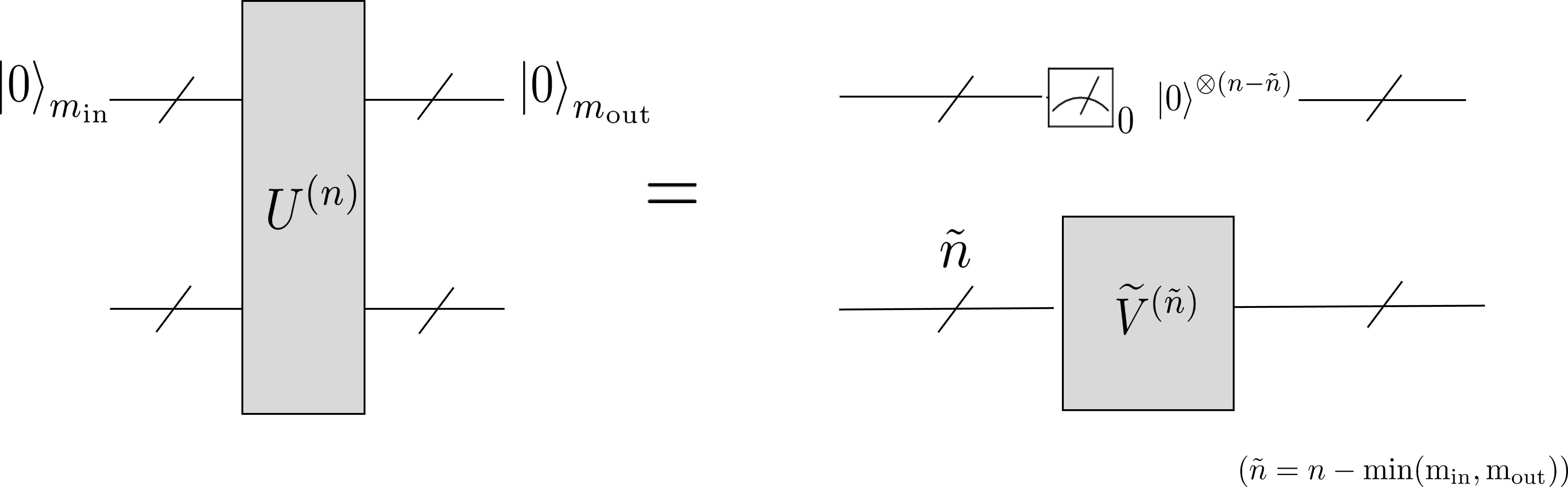
Figure 3: Schematic picture of corollary 1. This is the specific case of Fig. 2 where $P_{\rm{in}}$ and $P_{\rm{out}}$ are given by Eqs. (32) and (33), respectively.

Let us consider the case where the first $m_{\mathrm{in}}$ and $m_{\mathrm{out}}$ qubits of the input and output states are specified to be $\ket{0}$ (Figure 3). The pre- and post-selection of the quantum channel is described by

$$P_{\mathrm{in}} \,=\,\ket{0}\!\!\bra{0}^{\otimes m_{\mathrm{in}}}\otimes I^{\otimes(n-m_{\mathrm{in}})}_{2}\,=\,\begin{pmatrix}I_{r_{\mathrm{in}}}&\phantom{I_{r_{\mathrm{in}}}}\\ \phantom{I_{r_{\mathrm{in}}}}&\phantom{I_{r_{\mathrm{in}}}}\\ \end{pmatrix}\,,$$ (32)

$$P_{\mathrm{out}} \,=\,\ket{0}\!\!\bra{0}^{\otimes m_{\mathrm{out}}}\otimes I^{\otimes(n-m_{\mathrm{out}})}_{2}\,=\,\begin{pmatrix}I_{r_{\mathrm{out}}}&\phantom{I_{r_{\mathrm{out}}}}\\ \phantom{I_{r_{\mathrm{out}}}}&\phantom{I_{r_{\mathrm{out}}}}\\ \end{pmatrix}\,,$$ (33)

with

$$r_{\mathrm{in}}\,=\,2^{n-m_{\mathrm{in}}}\,,\quad r_{\mathrm{out}}\,=\,2^{n-m_{\mathrm{out}}}\,.$$ (34)

Since both the $P_{\mathrm{in}}$ and $P_{\mathrm{out}}$ have the same structure as $P_{d,\mathrm{in}}$ and $P_{d,\mathrm{out}}$ in Eqs. (20) and (21), we can take

$$O_{\mathrm{in}}=O_{\mathrm{out}}=I_{N}\,.$$ (35)

The explicit form of $\widetilde{V}^{(\tilde{n})}$ depends on whether $m_{\mathrm{out}}$ is larger than $m_{\mathrm{in}}$ or not. If $m_{\mathrm{out}}\leq m_{\mathrm{in}}$, then $\tilde{n}=n-m_{\mathrm{out}}$ and

$$\widetilde{V}^{(\tilde{n})}\,=\,\begin{pmatrix}(v_{1})_{1}&\cdots&(v_{r_{\mathrm{in}}})_{1}&0&\cdots&0\\ \vdots&&\vdots&\vdots&&\vdots\\ &\ddots&\vdots&&\ddots&\\ \vdots&&\vdots&\vdots&&\vdots\\ (v_{1})_{r_{\mathrm{out}}}&\cdots&(v_{r_{\mathrm{in}}})_{r_{\mathrm{out}}}&0&\cdots&0\\ \end{pmatrix}\,.$$ (36)

If $m_{\mathrm{out}}>m_{\mathrm{in}}$, then $\tilde{n}=n-m_{\mathrm{in}}$ and

$$\widetilde{V}^{(\tilde{n})}\,=\,\begin{pmatrix}(v_{1})_{1}&\cdots&&\cdots&(v_{r_{\mathrm{in}}})_{1}\\ \vdots&&\ddots&&\vdots\\ (v_{1})_{r_{\mathrm{out}}}&\cdots&&\cdots&(v_{r_{\mathrm{in}}})_{r_{\mathrm{out}}}\\ 0&\cdots&&\cdots&0\\ \vdots&&\ddots&&\vdots\\ 0&\cdots&&\cdots&0\\ \end{pmatrix}\,.$$ (37)

In both cases, the matrix element is given as

$$(v_{i})_{j}=\langle\langle\,E_{ji}|U^{(n)}\,\rangle\rangle\,.$$ (38)

We then arrive at the following corollary:

Corollary 1.

The $n$-qubit quantum channel $[P_{\mathrm{out}}U^{(n)}P_{\mathrm{in}}]$ where $P_{\mathrm{in}}$ and $P_{\mathrm{out}}$ are defined by Eqs. (32) and (33) satisfies

$$[P_{\mathrm{out}}U^{(n)}P_{\mathrm{in}}]\,=\,[\ket{0}\!\!\bra{0}^{\otimes(n-\tilde{n})}\widetilde{V}^{(\tilde{n})}]$$ (39)

where $\tilde{n}=n-\min(m_{\mathrm{in}},m_{\mathrm{out}})$. If $m_{\mathrm{out}}\leq m_{\mathrm{in}}$, $\tilde{V}^{(\tilde{n})}$ is calculated from Eqs. (36) and (38). If $m_{\mathrm{out}}>m_{\mathrm{in}}$, it is calculated from Eqs. (37) and (38).

The schematic picture of Corollary 1 is shown in Fig. 3.

III.2.2 Example 2

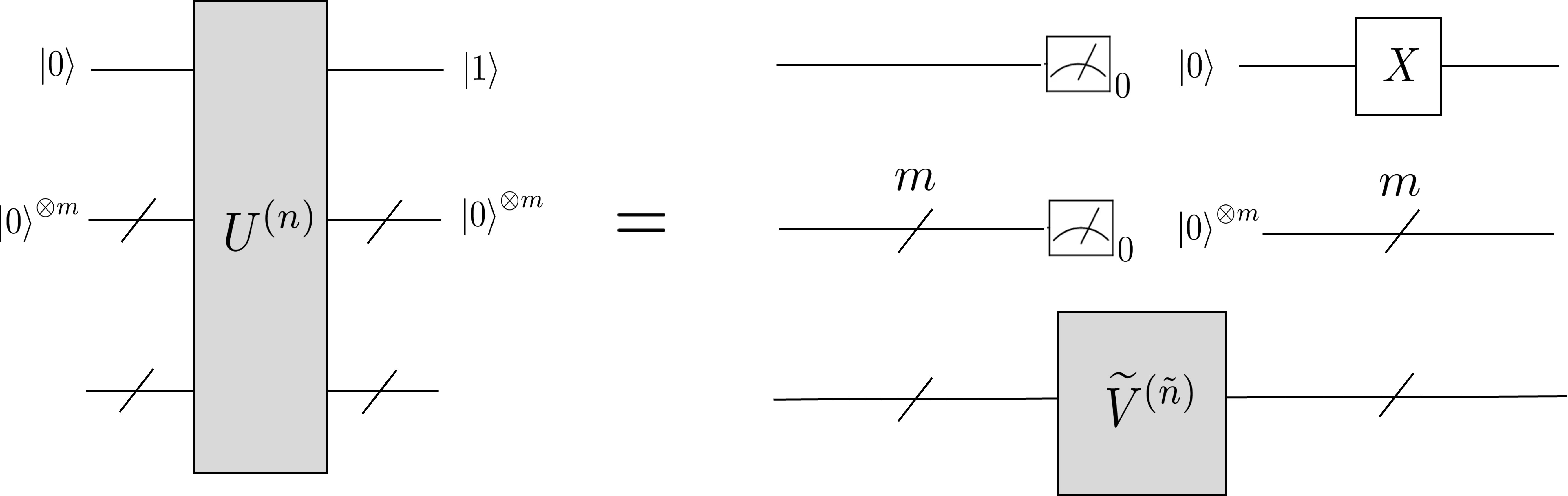
Figure 4: Schematic picture of Corollary 2. This is the specific case of Fig. 2 where $P_{\rm{in}}$ and $P_{\rm{out}}$ are given by Eqs. (40) and (41), respectively. HHL circuit (which is discussed in Section IV) falls into this case.

We next consider the case depicted in Fig. 4: The first $(m+1)$-qubits of the input state are set to be $\ket{0}$. For the output state, the first qubit is specified as $\ket{1}$ and the second to $(m+1)$th qubit are specified as $\ket{0}$. The quantum circuit of the HHL algorithm, which is discussed later, falls into this type.

The pre- and post-selection of the quantum channel is described by

$$P_{\mathrm{in}} =\ket{0}\!\!\bra{0}^{\otimes(m+1)}\otimes I^{\otimes(n-m-1)}\,=\,\begin{pmatrix}I_{r_{\mathrm{in}}}&\phantom{I_{r_{\mathrm{in}}}}\\ \phantom{I_{r_{\mathrm{in}}}}&\phantom{I_{r_{\mathrm{in}}}}\\ \end{pmatrix}\,,$$ (40)

$$P_{\mathrm{out}} =\ket{1}\!\!\bra{1}\otimes\ket{0}\!\!\bra{0}^{\otimes m}\otimes I^{\otimes(n-m-1)}$$

$$\,=\,\begin{pmatrix}0_{2^{n-1}}&\phantom{I_{r_{\mathrm{in}}}}&\phantom{I_{r_{\mathrm{in}}}}\\ \phantom{I_{r_{\mathrm{in}}}}&I_{r_{\mathrm{out}}}&\phantom{I_{r_{\mathrm{in}}}}\\ \phantom{I_{r_{\mathrm{in}}}}&\phantom{I_{r_{\mathrm{in}}}}&\phantom{I_{r_{\mathrm{in}}}}\end{pmatrix}\,,$$ (41)

with $0_{m}$ being $m\times m$ zero matrix and

$$r_{\mathrm{in}}\,=\,r_{\mathrm{out}}\,=\,2^{n-m-1}\,:=\,r\,.$$ (42)

Since $P_{\mathrm{in}}$ is the matrix with the same structure as $P_{d,\mathrm{in}}$ (Eq. (20)), we take

$$O_{\mathrm{in}}=I_{N}\,.$$ (43)

On the other hand, $P_{\mathrm{out}}$ is the diagonal matrix but the structure is different from $P_{d,\mathrm{out}}$ (Eq. (21)). To make $P_{\mathrm{out}}$ have the same structure as $P_{d,\mathrm{out}}$, we perform unitary transformation by

$$O_{\mathrm{out}} \,=\,X\otimes I^{\otimes(n-1)}\,.$$ (44)

The effective number of qubits $\tilde{n}$ is given as

$$\tilde{n}=n-m-1\,.$$ (45)

The effective operation $\widetilde{V}^{(\tilde{n})}$ is calculated as

$$\widetilde{V}^{(\tilde{n})}\,=\,\begin{pmatrix}(v_{1})_{1}&\cdots&(v_{1})_{r}\\ \vdots&\ddots&\vdots\\ (v_{r})_{1}&\cdots&(v_{r})_{r}\\ \end{pmatrix}\,,$$ (46)

where

$$(v_{i})_{j} \,=\,\langle\langle\,E_{ji}|O_{\mathrm{out}}U^{(n)}\,\rangle\rangle$$

$$\,=\,\langle\langle\,O^{\dagger}_{\mathrm{out}}E_{ji}|U^{(n)}\,\rangle\rangle$$

$$\,=\,\langle\langle\,E_{k_{j}i}|U^{(n)}\,\rangle\rangle\,,$$ (47)

with $k_{j}=(2^{n-1}+j-1)\,\mathrm{mod}\,2^{n}+1$.

We arrive at the following corollary:

Corollary 2.

The $n$-qubit quantum channel $[P_{\mathrm{out}}U^{(n)}P_{\mathrm{in}}]$ where $P_{\mathrm{in}}$ and $P_{\mathrm{out}}$ are defined by Eqs. (40) and (41) can be equivalently expressed as

$$[P_{\mathrm{out}}U^{(n)}P_{\mathrm{in}}]$$

$$\,=\,[(X\otimes I^{\otimes(n-1)})(\ket{0}\!\!\bra{0}^{\otimes(n-\tilde{n})}\widetilde{V}^{(\tilde{n})})]\,,$$ (48)

where $\tilde{n}=n-m$ and $\widetilde{V}^{(\tilde{n})}$ is given by Eqs. (46) and (47)

The schematic picture of corollary 2 is shown in Fig. 4.

III.3 Gate decomposition with pre- and post-selection

As we discussed above, the $n$-qubit channel with pre- and post-selection, $[P_{\mathrm{out}}U^{(n)}P_{\mathrm{in}}]$, is characterized by $\tilde{n}$-qubit channel, $[\widetilde{V}^{(\tilde{n})}]$. We here perform the gate decomposition (6) to $[\widetilde{V}^{(\tilde{n})}]$ as

$$[\widetilde{V}^{(\tilde{n})}]\,=\,\sum_{i=1}^{\tilde{D}}c_{i}\,[V^{(1)}_{i_{1}}\otimes\cdots\otimes V^{(1)}_{i_{\tilde{n}}}]\,,$$ (49)

with $i=\sum_{k=1}^{\tilde{n}}(\prod_{k^{\prime}=1}^{k}D_{k^{\prime}-1})i_{k}$. We note that $\widetilde{D}$ needs to be only larger than $16^{\tilde{n}}$ which is generally smaller than $N^{4}=16^{n}$.

Combining Eq. (49) with Theorem 1, we find the following fact:

Theorem 2.

Let $P_{\mathrm{in}}$ and $P_{\mathrm{out}}$ be projection matrices with ${\mathrm{rank}}P_{\mathrm{in}}=r_{\mathrm{in}}$ and ${\mathrm{rank}}P_{\mathrm{out}}=r_{\mathrm{out}}$. The $n$-qubit quantum channel with the pre- and post-selection, $[P_{\mathrm{out}}U^{(n)}P_{\mathrm{in}}]$, is decomposed as

$$[P_{\mathrm{out}}U^{(n)}P_{\mathrm{in}}]$$

$$\,=\,\sum_{i=1}^{\widetilde{D}}c_{i}\,[O_{\mathrm{out}}(\ket{0}\!\!\bra{0}^{\otimes(n-\tilde{n})}\otimes V^{(1)}_{i_{1}}\otimes\cdots\otimes V^{(1)}_{i_{\tilde{n}}})O_{\mathrm{in}}]\,,$$ (50)

where $i=\sum_{k=1}^{\tilde{n}}(\prod_{k^{\prime}=1}^{k}D_{k^{\prime}-1})i_{k}$ with $D_{0}=1$, $\tilde{n}=\lceil{\log_{2}{\mathrm{max}}(r_{\mathrm{in}},r_{\mathrm{out}})\rceil}$, and $\{V^{(1)}_{i_{a}}\,,(a=1,\cdots,\tilde{n})\}$ denotes the set of linearly independent one-qubit quantum channels. We need $\widetilde{D}\geq 16^{\tilde{n}}$ to satisfy the equality. $O_{\mathrm{in}}$ and $O_{\mathrm{out}}$ are the unitary matrices defined as Eqs. (20) and (21).

As the demonstration, we perform the gate decomposition (50) of Toffoli and the three-qubit QFT gate with pre- and post-selection. Here we consider the case where $P_{\rm{in}}=\ket{0}\!\!\bra{0}^{\otimes m_{\rm{in}}}\otimes I^{(3-m_{\rm{in}})}$ and $P_{\rm{out}}=\ket{0}\!\!\bra{0}^{\otimes m_{\rm{out}}}\otimes I^{(3-m_{\rm{out}})}$ with $0\leq m_{\rm{in}},m_{\rm{out}}\leq 3$. This is the case discussed in Section III.2.1. To obtain the coefficients $\{c_{i}\}$, we calculate $\widetilde{V}^{(\tilde{n})}$ using Corollary 1 and solve Eq. (49). The resulting sampling overheads $\gamma=\sum_{i}|c_{i}|$ are presented in Tables 2 and 3.

Table 2: Sampling overhead $\gamma=\sum_{i=1}|c_{i}|$ for the decomposition of Toffoli gate with pre- and post-selection. $\ket{abc}=\ket{a}\otimes\ket{b}\otimes\ket{c}$ and $\ket{*}$ denotes an arbitrary one-qubit pure state.

	$\ket{***}$	$\ket{0**}$	$\ket{00*}$	$\ket{000}$
$\ket{***}$	37	37	37	37
$\ket{0**}$	37	1	1	1
$\ket{00*}$	37	1	1	1
$\ket{000}$	37	1	1	1

Table 3: Sampling overhead $\gamma=\sum_{i=1}|c_{i}|$ for the decomposition of the three-qubit QFT gate with pre- and post-selection. $\ket{abc}=\ket{a}\otimes\ket{b}\otimes\ket{c}$ and $\ket{*}$ denotes an arbitrary one-qubit pure state.

	$\ket{***}$	$\ket{0**}$	$\ket{00*}$	$\ket{000}$
$\ket{***}$	261.43	261.43	261.43	261.43
$\ket{0**}$	261.43	261.43	16.63	16.63
$\ket{00*}$	261.43	16.63	1.64	1.64
$\ket{000}$	261.43	16.63	1.64	1

We observe that the pre- and post-selection reduces the cost of the gate decomposition.

IV Numerical experiments

The gate decomposition method allows us to simulate a complicated quantum circuit by sampling the outputs of relatively simpler quantum circuits. The gate decomposition is therefore expected to reduce the impact of errors during the quantum computation. In this section, we actually demonstrate this benefit of the gate decomposition.

We here study the HHL algorithm [27, 33, 34, 35, 36, 37, 38]. Since the HHL algorithm requires the pre- and post-selections on many ancilla qubits, the advantage of our decomposition method should be manifest.

IV.1 Harrow-Hassidim-Lloyd (HHL) algorithm

Here we briefly describe the HHL algorithm. This is a quantum algorithm to solve the linear equation, $A\vec{x}=\vec{b}$. Here $A$ and $\vec{b}$ denote a $\tilde{N}\times\tilde{N}$ complex matrix and a $\tilde{N}$-dimensional complex vector, respectively. The algorithm produces an approximating solution of a certain type of function of $\vec{x}$ (e.g., $\vec{x}^{\dagger}H\vec{x}$ with $H$ a Hermitian matrix), with running time of $\mathcal{O}({\rm{poly}}{\rm{log}}{\tilde{N}})$ when $A$ is sparse, while any classical computation needs $\mathcal{O}({\tilde{N}})$ running time.

The basic quantum circuit of the HHL is shown in Fig. 5. The algorithm needs $n=\tilde{n}+m+1$ qubits where $\tilde{n}$-qubits are used for the amplitude encoding of $\vec{b}$ and the $(m+1)$-qubits are used as ancilla. The $m$-ancilla qubits are used to store the binary representation of the eigenvalues of $A$, and the rest one ancilla qubit is used to encode the inverse of the eigenvalues of the matrix. All ancilla qubits are set to be $\ket{0}$ at the beginning (pre-selection), and they are post-selected as $\ket{1}\otimes\ket{0}^{\otimes m}$. With this post-selection, we obtain the solution state $\ket{\vec{x}}$ up to a normalization factor $c$ in the working qubits.

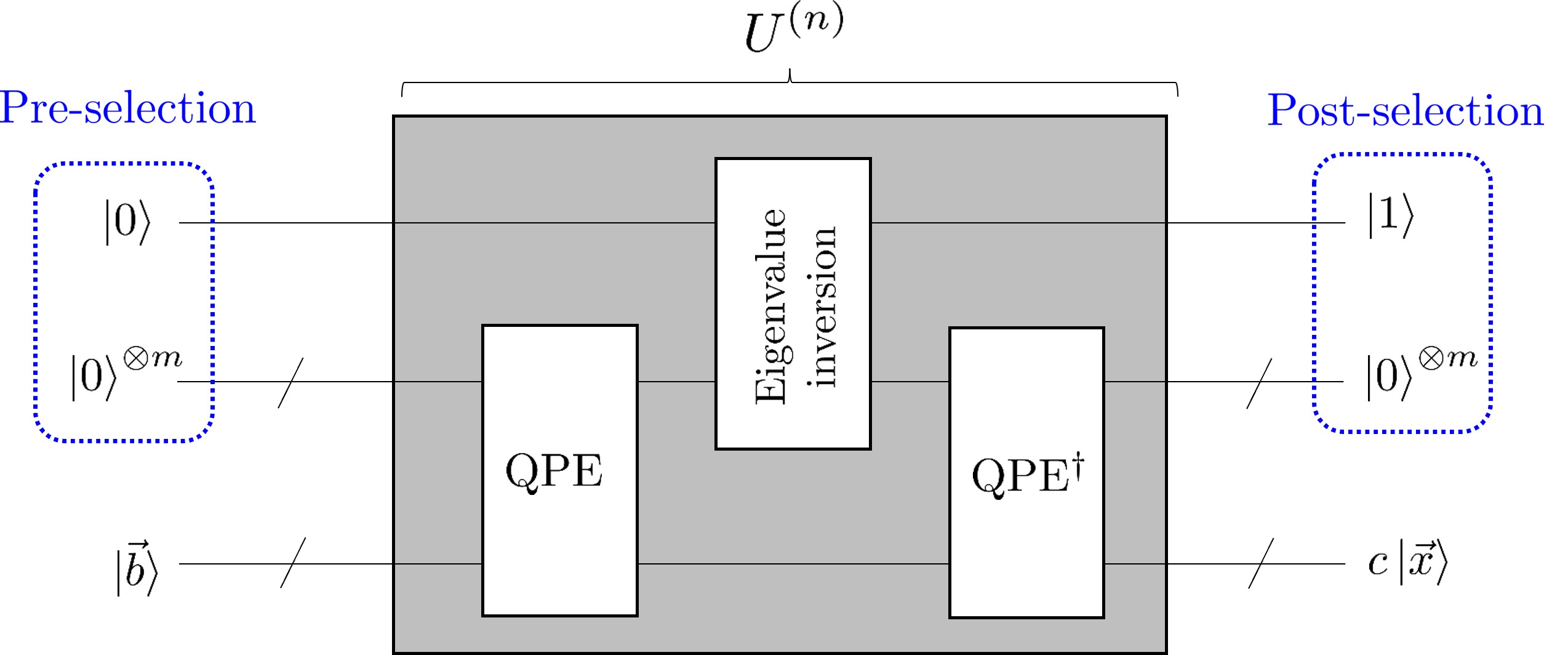
Figure 5: Quantum circuit of the HHL algorithm for solving $A\vec{x}=\vec{b}$. The first $(m+1)$ qubits are used as ancilla qubits which are initialized to be $\ket{0}^{\otimes(m+1)}$ (pre-selection). The unitary operation $U^{(n)}$ has three steps: (i) Quantum Phase Estimation (QPE), (ii) conditional rotation to encode the inverse of the eigenvalues of $A$, and (iii) uncomputation (QPE^†). With this post-selection of the ancilla qubits as the $\ket{1}\otimes\ket{0}^{\otimes m}$, we obtain the solution state $\vec{x}$ up to a normalization factor $c$ in the working qubits.

In our terminology, the quantum channel of HHL corresponds to the case discussed in Section III.2.2. The target unitary operation $U^{(n)}$ consists of the following three steps. First, it applies Quantum Phase Estimation (QPE) to obtain the binary representation of the eigenvalues of $A$. The eigenvalues are stored in the middle $m$-ancilla qubits. Second, the conditional rotation is performed to get the inverse eigenvalues of $A$. The information of the inverse eigenvalues is stored in the coefficient of $\ket{1}$ of the first ancilla qubit. Third, we apply QPE^† for the uncomputation.

It should be noted that the HHL requires huge resources in general. As we will see below, even in the simplest $(\tilde{N}=2)$ case, the quantum circuit typically has hundreds of depths and requires tens of CNOTs. This implies that the quantum computation seriously suffers from huge errors. In the next subsection, we perform the gate decomposition of the HHL circuit and demonstrate that it drastically reduces the effect of error.

IV.2 Gate decomposition of HHL circuit

Here we study the HHL algorithm for solving $A\vec{x}=\vec{b}$ with

$$A\,=\,\begin{pmatrix}1&-1/3\\ -1/3&1\end{pmatrix}\,,\quad\vec{b}=\begin{pmatrix}1\\ 0\end{pmatrix}\,.$$ (51)

This corresponds to the case of $\tilde{n}=1$ ($\tilde{N}=2$).

We used Qiskit [39] to simulate the HHL circuit. In particular, we generated the quantum circuit by using linear_solvers package in Qiskit. The depth of the resulting circuit is 212, and it contains 108 CNOT gates. Also, $m=3$ ancilla qubits are used to store the eigenvalues of $A$. The quantum circuit has, therefore, $n=1+3+1=5$ qubit in total.

First, we show the simulation result of the HHL algorithm without the gate decomposition. We estimated the output state by performing the state tomography simulation (with 10000 shots) using Qiskit. The post-selection is implemented by extracting the relevant components of the output state. If the algorithm correctly works, the extracted density matrix $\rho_{\rm{out}}$ ends up with $\rho_{\rm{sol}}=\ket{\vec{x}}\!\!\bra{\vec{x}}$ with $\ket{\vec{x}}=\ket{A^{-1}\vec{b}}=[9/8,3/8]^{T}$ up to constant. To evaluate the performance of the algorithm, we used state_fidelity function in Qiskit to compute the fidelity $\mathcal{F}$ between the normalized output state $\hat{\rho}_{\rm{out}}={\rho}_{\rm{out}}/\mbox{Tr}({\rho}_{\rm{out}})$ and the solution state $\hat{\rho}_{\rm{sol}}={\rho}_{\rm{sol}}/\mbox{Tr}({\rho}_{\rm{sol}})$. Also, we consider the case with and without quantum noise. In the simulation with the noise, we assume that the one-qubit depolarization error occurs with probability $p_{\rm{local}}=0.001$ for one-qubit gates and $p_{\rm{CNOT}}=0.005,~{}0.01$ for CNOT gates. The results of the fidelity $\mathcal{F}$ are shown in the top row of Table 4 indicated by ”w/o decomposition”. In the case without noise (i.e., $p_{\rm{local}}=p_{\rm{CNOT}}=0$), we observe $\mathcal{F}\simeq 0.99$, which ensures that the HHL algorithm works well; note that the small deviation from the ideal value $\mathcal{F}=1$ is due to the statistical error in the state tomography. In contrast, the fidelity gets worse as $\mathcal{F}\simeq 0.86$ and $\mathcal{F}\simeq 0.75$ for the cases $p_{\rm{CNOT}}=0.005$ and $p_{\rm{CNOT}}=0.01$, respectively. This is simply because there are too many CNOT gates in the HHL circuit and they all seriously suffer from the noise.

Table 4: Fidelity $\mathcal{F}$ between the output state of the HHL and the solution state with and without the gate decomposition. If the HHL algorithm perfectly works, the value of fidelity becomes unity. The noise is assumed to be the one-qubit depolarization error with the error probability $p_{\rm{local}}=0.001$ for one-qubit gates and $p_{\rm{CNOT}}=0.005$ and $0.01$ for CNOT gate. The noise-free case $p_{\rm{local}}=p_{\rm{CNOT}}=0$ is also shown.

	Noise-free	$p_{\rm{CNOT}}=0.005$	$p_{\rm{CNOT}}=0.01$
w/o decomposition	0.99	0.86	0.75
w/ decomposition	0.99	0.99	0.99

We next study the performance of the gate-decomposed HHL circuit. As mentioned before, the quantum channel of the HHL algorithm is included in the class of channels discussed in Section III.2.2. Specifically, $\tilde{n}=1$ in our case. We first compute the effective operation $\widetilde{V}^{(\tilde{n})}$ given in Eqs. (46) and (47). Then, Eq. (49) is solved to obtain the coefficients $\{c_{i}\}$, where the basis in Table 1 is employed. The result is that

$$[\widetilde{V}^{(\tilde{n})}]\,=\,\frac{3}{8}[I]-\frac{1}{8}[X]+\frac{6}{8}[\pi_{X}]\,,$$ (52)

which leads to

$$[ P_{\rm{out}}U^{(n)}P_{\rm{in}}]$$

$$\,= \,\frac{3}{8}[(X\otimes I\otimes I\otimes I\otimes I)(\pi_{Z}\otimes\pi_{Z}\otimes\pi_{Z}\otimes\pi_{Z}\otimes I)]$$

$$\,-\frac{1}{8}[(X\otimes I\otimes I\otimes I\otimes I)(\pi_{Z}\otimes\pi_{Z}\otimes\pi_{Z}\otimes\pi_{Z}\otimes X)]$$

$$\,+\frac{6}{8}[(X\otimes I\otimes I\otimes I\otimes I)(\pi_{Z}\otimes\pi_{Z}\otimes\pi_{Z}\otimes\pi_{Z}\otimes\pi_{X})]\,.$$ (53)

Therefore, notably, the original HHL circuit, which is of depth 212 and contains 108 CNOT gates, can be decomposed to only three channels each of which is of depth 2 and does not contains any CNOT gate. Because those three channels are expected to be almost free from noise, nearly ideal simulation might be possible. Furthermore, fortunately, the number of decomposition is only $\tilde{D}=3$, while in general $\tilde{D}\geq 16^{\tilde{n}}=16$ is required for the case $\tilde{n}=1$ (note thus that 13 of total 16 coefficients $\{c_{i}\}$ are all zero). As a result, the sampling overhead is only $\gamma=5/4$, meaning that the virtual simulation via the channel decomposition can be efficiently executed with low sampling overhead.

We also calculate the sampling costs for particular larger-dimensional cases where

$$A \,=\,\begin{pmatrix}1&-\frac{1}{3}&0&0\\ -\frac{1}{3}&1&-\frac{1}{3}&0\\ 0&-\frac{1}{3}&1&-\frac{1}{3}\\ 0&0&-\frac{1}{3}&1\end{pmatrix}\,,$$ (54)

$$A \,=\,\begin{pmatrix}1&-\frac{1}{3}&0&0&0&0&0&0\\ -\frac{1}{3}&1&-\frac{1}{3}&0&0&0&0&0\\ 0&-\frac{1}{3}&1&-\frac{1}{3}&0&0&0&0\\ 0&0&-\frac{1}{3}&1&-\frac{1}{3}&0&0&0\\ 0&0&0&-\frac{1}{3}&1&-\frac{1}{3}&0&0\\ 0&0&0&0&-\frac{1}{3}&1&-\frac{1}{3}&0\\ 0&0&0&0&0&-\frac{1}{3}&1&-\frac{1}{3}\\ 0&0&0&0&0&0&-\frac{1}{3}&1\\ \end{pmatrix}\,,$$ (55)

and $\vec{b}=(1,0,\cdots,0)^{T}$. These cases respectively correspond to $\tilde{n}=2$ and $\tilde{n}=3$. The resulting sampling costs are $\gamma\simeq 4.7$ for Eq. (54) and $\gamma\simeq 16.5$ for Eq. (55). Unfortunately, we cannot obtain the analytic form of the decomposition and accordingly the $\gamma$ factors in $\tilde{n}\geq 2$ cases. This numerical results implies that the sampling cost scales exponentially with $\tilde{n}$, but the scaling is much milder than $16^{n}$.

The decomposing channels represented in the right-hand side of Eq. (53) are products of one-qubit channels and thus easy to implement. But implementation of the developed channel is easier than expected, because the ancilla qubits are initialized as $\ket{0000}$ in the HHL algorithm. Actually, in this case, the operation on the ancilla qubits is trivial and thus can be ignored, meaning that we only need to implement the one-qubit decomposed gate (52). $[\pi_{X}]$ can be implemented as measure-and-prepare channel because $\pi_{X}=\ket{+}\!\!\bra{+}$.

We can now give a quantitative discussion on the benefit of the gate decomposition, from the view of noise-tolerance property. Let us assume the same error model as in the analysis without the gate decomposition. We summarize the state fidelity with the gate decomposition in the bottom row of Table 4. Likewise the w/o decomposition case, $\mathcal{F}\simeq 0.99$ is achieved in the noise-free case $p_{\rm{local}}=p_{\rm{CNOT}}=0$, implying that the gate decomposition is successfully executed. A notable difference to the previous case is found in the noisy cases $p_{\rm{local}}=0.001$, $p_{\rm{CNOT}}=0.005$ and $p_{\rm{CNOT}}=0.01$. That is, even in this case the state fidelity $\mathcal{F}$ remains close to unity, demonstrating the effectiveness of the gate decomposition method against noise.

V Conclusion

The channel-decomposition technique is useful, but it suffers from the exponential increase of the number of decompositions, or equivalently the sampling overhead $\gamma$, with respect to the size of the target channel. This paper proposed a general method for reducing this cost by focusing on channels with pre- and post-selection, i.e., the channels whose input and output are restricted to fixed set of states. We proved that the overhead is determined by the rank of projection operators specifying the input and output states. Also, the form of decomposition under the pre- and post-selection is explicitly given. As a demonstration, we applied the method to decompose the unitary operator for the HHL algorithm, showing an efficient channel decomposition (or equivalently low sampling overhead) thanks to the pre- and post-selection.

There are many examples of channels with pre- and post-selection to which the proposed method is applicable. A typical example is a gate for probabilistic state preparation, because the quantum operation is embedded into the larger unitary gate and is implemented by pre- and post-selections of ancilla qubits. The probabilistic imaginary time evolution, which can be used for quantum chemistry, also falls into this class [40, 41, 42]. The differential equation solvers [43, 44, 45, 46, 47], which can be used for finance [48, 49], may also be a relevant target to be investigated because they are based on the HHL algorithm. Finally, to extend the class of target channels, we need to develop a gadget for systematically decomposing a small part of the entire circuit, such as the Toffoli gate contained in the circuit for the factorization algorithm [50].

Appendix A Gate decomposition of CNOT and Toffoli gates

Here we give the expressions of the gate decomposition of CNOT and Toffoli gates in Eqs. (7) and (8), respectively. The three-qubit QFT gate in Eq. (9) is decomposed to 1524 channels, and thus we do not show those terms here.

CNOT gate can be decomposed as [2]

$$[U^{(n)}] \,=\,-\frac{1}{2}[IR_{X}]+\frac{1}{2}[IX]+[I\pi_{X}]-\frac{1}{2}[R_{Z}I]$$

$$+[R_{Z}R_{X}]-\frac{1}{2}[R_{Z}X]+\frac{1}{2}[ZI]-\frac{1}{2}[ZR_{X}]$$

$$+[ZX]-[Z\pi_{X}]+[\pi_{Z}I]-[\pi_{Z}X]\,,$$ (56)

where $[AB]$ means $[A\otimes B]$. The corresponding overhead is $\gamma=\sum_{i}|c_{i}|=9$ .

Toffoli gate can be decomposed as

$$[U^{(n)}] \,=\,\frac{3}{4}[IR_{Z}R_{X}]+\frac{3}{4}[R_{Z}IR_{X}]+\frac{1}{2}[I\pi_{Z}R_{X}]+\frac{1}{2}[\pi_{Z}IR_{X}]$$

$$-\frac{1}{2}[IZR_{X}]-\frac{1}{2}[ZIR_{X}]-\frac{3}{4}[IIR_{X}]+\frac{1}{2}[IR_{Z}\pi_{X}]$$

$$+\frac{1}{2}[R_{Z}I\pi_{X}]+\frac{1}{2}[R_{Z}\pi_{Z}I]+\frac{1}{2}[\pi_{Z}R_{Z}I]-\frac{1}{2}[IR_{Z}X]$$

$$-\frac{1}{2}[R_{Z}IX]-\frac{1}{2}[R_{Z}ZI]-\frac{1}{2}[ZR_{Z}I]-\frac{3}{4}[IR_{Z}I]$$

$$-\frac{3}{4}[R_{Z}II]+\frac{3}{4}[R_{Z}R_{Z}I]-[I\pi_{Z}\pi_{X}]-[\pi_{Z}I\pi_{X}]$$

$$+[II\pi_{X}]+[I\pi_{Z}I]+[\pi_{Z}II]-[\pi_{Z}\pi_{Z}I]$$

$$-\frac{1}{2}[I\pi_{Z}X]-\frac{1}{2}[\pi_{Z}IX]+\frac{5}{8}[IZX]+\frac{5}{8}[ZIX]$$

$$+\frac{3}{8}[IIX]-\frac{1}{2}[IZ\pi_{X}]-\frac{1}{2}[ZI\pi_{X}]-\frac{1}{2}[Z\pi_{Z}I]$$

$$-\frac{1}{2}[\pi_{Z}ZI]+\frac{3}{8}[IZI]+\frac{3}{8}[ZII]+\frac{5}{8}[ZZI]$$

$$+\frac{3}{8}[III]-[R_{Z}\pi_{Z}R_{X}]-[\pi_{Z}R_{Z}R_{X}]+\frac{1}{4}[R_{Z}ZR_{X}]$$

$$+\frac{1}{4}[ZR_{Z}R_{X}]+\frac{1}{2}[Z\pi_{Z}R_{X}]+\frac{1}{2}[\pi_{Z}ZR_{X}]-\frac{1}{4}[ZZR_{X}]$$

$$-[R_{Z}R_{Z}\pi_{X}]+\frac{1}{2}[R_{Z}\pi_{Z}X]+\frac{1}{2}[\pi_{Z}R_{Z}X]-\frac{1}{4}[R_{Z}ZX]$$

$$-\frac{1}{4}[ZR_{Z}X]+\frac{1}{4}[R_{Z}R_{Z}X]+\frac{1}{2}[R_{Z}Z\pi_{X}]+\frac{1}{2}[ZR_{Z}\pi_{X}]$$

$$+[\pi_{Z}\pi_{Z}X]-[Z\pi_{Z}X]-[\pi_{Z}ZX]+\frac{5}{8}[ZZX]$$

$$+[Z\pi_{Z}\pi_{X}]+[\pi_{Z}Z\pi_{X}]-[ZZ\pi_{X}]\,,$$ (57)

where $[ABC]$ means $[A\otimes B\otimes C]$. The corresponding overhead is $\gamma=\sum_{i}|c_{i}|=37$ .

References

• Temme et al. [2017] K. Temme, S. Bravyi,  and J. M. Gambetta, Physical review letters 119, 180509 (2017).
• Endo et al. [2018] S. Endo, S. C. Benjamin,  and Y. Li, Physical Review X 8, 031027 (2018).
• Takagi [2021] R. Takagi, Physical Review Research 3, 033178 (2021).
• Piveteau et al. [2022] C. Piveteau, D. Sutter,  and S. Woerner, npj Quantum Information 8, 12 (2022).
• Bravyi et al. [2016] S. Bravyi, G. Smith,  and J. A. Smolin, Physical Review X 6, 021043 (2016).
• Mitarai and Fujii [2021a] K. Mitarai and K. Fujii, New Journal of Physics 23, 023021 (2021a).
• Mitarai and Fujii [2021b] K. Mitarai and K. Fujii, Quantum 5, 388 (2021b).
• Marshall et al. [2022] S. Marshall, C. Gyurik,  and V. Dunjko, CoRR abs/2203.13739  (2022).
• Piveteau and Sutter [2022] C. Piveteau and D. Sutter, arXiv preprint arXiv:2205.00016  (2022).
• Takeuchi et al. [2022] Y. Takeuchi, Y. Takahashi, T. Morimae,  and S. Tani, Quantum 6, 758 (2022).
• Bechtold et al. [2023] M. Bechtold, J. Barzen, F. Leymann, A. Mandl, J. Obst, F. Truger,  and B. Weder, arXiv preprint arXiv:2302.01792  (2023).
• Peng et al. [2020] T. Peng, A. W. Harrow, M. Ozols,  and X. Wu, Physical review letters 125, 150504 (2020).
• Perlin et al. [2021] M. A. Perlin, Z. H. Saleem, M. Suchara,  and J. C. Osborn, npj Quantum Information 7, 64 (2021).
• Ayral et al. [2020] T. Ayral, F.-M. Le Régent, Z. Saleem, Y. Alexeev,  and M. Suchara, in 2020 IEEE Computer Society Annual Symposium on VLSI (ISVLSI) (IEEE, 2020) pp. 138–140.
• Tang et al. [2021] W. Tang, T. Tomesh, M. Suchara, J. Larson,  and M. Martonosi, in Proceedings of the 26th ACM International conference on architectural support for programming languages and operating systems (2021) pp. 473–486.
• Ying et al. [2023] C. Ying, B. Cheng, Y. Zhao, H.-L. Huang, Y.-N. Zhang, M. Gong, Y. Wu, S. Wang, F. Liang, J. Lin, et al., Physical review letters 130, 110601 (2023).
• Tang and Martonosi [2022] W. Tang and M. Martonosi, arXiv preprint arXiv:2207.00933  (2022).
• Uchehara et al. [2022] G. Uchehara, T. M. Aamodt,  and O. Di Matteo, arXiv preprint arXiv:2211.07358  (2022).
• Chen et al. [2022] D. Chen, B. Baheri, V. Chaudhary, Q. Guan, N. Xie,  and S. Xu, arXiv preprint arXiv:2212.01270  (2022).
• Lowe et al. [2023] A. Lowe, M. Medvidović, A. Hayes, L. J. O’Riordan, T. R. Bromley, J. M. Arrazola,  and N. Killoran, Quantum 7, 934 (2023).
• Ufrecht et al. [2023] C. Ufrecht, M. Periyasamy, S. Rietsch, D. D. Scherer, A. Plinge,  and C. Mutschler, arXiv preprint arXiv:2302.00387  (2023).
• Brenner et al. [2023] L. Brenner, C. Piveteau,  and D. Sutter, arXiv preprint arXiv:2302.03366  (2023).
• Harada et al. [2023] H. Harada, K. Wada,  and N. Yamamoto, arXiv preprint arXiv:2303.07340  (2023).
• Pednault [2023] E. Pednault, arXiv preprint arXiv:2303.08287  (2023).
• Chen et al. [2023] D. T. Chen, E. H. Hansen, X. Li, V. Kulkarni, V. Chaudhary, B. Ren, Q. Guan, S. Kuppannagari, J. Liu,  and S. Xu, arXiv preprint arXiv:2304.04093  (2023).
• Grover [1996] L. K. Grover, in Proceedings of the twenty-eighth annual ACM symposium on Theory of computing (1996) pp. 212–219.
• Harrow et al. [2009] A. W. Harrow, A. Hassidim,  and S. Lloyd, Physical review letters 103, 150502 (2009).
• Horn and Johnson [2012] R. A. Horn and C. R. Johnson, Matrix analysis (Cambridge university press, 2012).
• de Pillis [1967] J. de Pillis, Pacific Journal of Mathematics 23, 129 (1967).
• Jamiołkowski [1972] A. Jamiołkowski, Reports on Mathematical Physics 3, 275 (1972).
• Choi [1975] M.-D. Choi, Linear algebra and its applications 10, 285 (1975).
• Bergholm [2015] V. Bergholm, arXiv preprint arXiv:1509.08339  (2015).
• Ambainis [2010] A. Ambainis, arXiv preprint arXiv:1010.4458  (2010).
• Childs et al. [2017] A. M. Childs, R. Kothari,  and R. D. Somma, SIAM Journal on Computing 46, 1920 (2017).
• Liu et al. [2023] J. Liu, M. Liu, J.-P. Liu, Z. Ye, Y. Alexeev, J. Eisert,  and L. Jiang, arXiv preprint arXiv:2303.03428  (2023).
• Dervovic et al. [2018] D. Dervovic, M. Herbster, P. Mountney, S. Severini, N. Usher,  and L. Wossnig, arXiv preprint arXiv:1802.08227  (2018).
• Morrell Jr et al. [2021] H. J. Morrell Jr, A. Zaman,  and H. Y. Wong, arXiv preprint arXiv:2108.09004  (2021).
• Tosti Balducci et al. [2022] G. Tosti Balducci, B. Chen, M. Möller, M. Gerritsma,  and R. De Breuker, Frontiers in Mechanical Engineering , 75 (2022).
• Qiskit contributors [2023] Qiskit contributors, “Qiskit: An open-source framework for quantum computing,”  (2023).
• Kosugi et al. [2022] T. Kosugi, Y. Nishiya, H. Nishi,  and Y.-i. Matsushita, Physical Review Research 4, 033121 (2022).
• Liu et al. [2021a] T. Liu, J.-G. Liu,  and H. Fan, Quantum Inf. Process. 20, 204 (2021a).
• Lin et al. [2021] S.-H. Lin, R. Dilip, A. G. Green, A. Smith,  and F. Pollmann, PRX Quantum 2, 010342 (2021).
• Berry [2014] D. W. Berry, Journal of Physics A: Mathematical and Theoretical 47, 105301 (2014).
• Berry et al. [2017] D. W. Berry, A. M. Childs, A. Ostrander,  and G. Wang, Communications in Mathematical Physics 356, 1057 (2017).
• Xin et al. [2020] T. Xin, S. Wei, J. Cui, J. Xiao, I. Arrazola, L. Lamata, X. Kong, D. Lu, E. Solano,  and G. Long, Physical Review A 101, 032307 (2020).
• Liu et al. [2021b] J.-P. Liu, H. Ø. Kolden, H. K. Krovi, N. F. Loureiro, K. Trivisa,  and A. M. Childs, Proceedings of the National Academy of Sciences 118, e2026805118 (2021b).
• An et al. [2022] D. An, J.-P. Liu, D. Wang,  and Q. Zhao, arXiv preprint arXiv:2211.05246  (2022).
• Rebentrost and Lloyd [2018] P. Rebentrost and S. Lloyd, arXiv preprint arXiv:1811.03975  (2018).
• Miyamoto and Kubo [2021] K. Miyamoto and K. Kubo, IEEE Transactions on Quantum Engineering 3, 1 (2021).
• Oonishi et al. [2022] K. Oonishi, T. Tanaka, S. Uno, T. Satoh, R. Van Meter,  and N. Kunihiro, IEEE Transactions on Quantum Engineering 3, 1 (2022).