Josephson-type oscillations in spin-orbit coupled Bose-Einstein condensates with nonlinear optical lattices

Abstract

We consider spin-orbit coupled Bose Einstein Condensate in presence of linear and nonlinear optical lattices within the framework of quasi-one-dimensional Gross-Pitaevskii equation. The population imbalance between the states changes periodically with time and the oscillation amplitude depends sensitively on the initial phase. The optical lattice is found to change phase velocity of the oscillation of population imbalance. This oscillation can also be arrested beyond critical values of parameters. We find that the optical lattice can efficiently be used to control the critical point.

I Introduction

Since the first experimental observation of BEC in 1995[1, 2], it has been playing a very important role both theoretically and experimentally for studying various topics related to many- body system, condensed matter and nonlinear physics. Ultracold atomic system serves as a good platform, primarily, because of it’s flexibility to tune different parameters. One of the greatest advance in this filed is the study of charge physics using neutral atoms. This leads to the realization of spin-orbit coupling in BECs [3, 4].

Mean-field interaction in Bose-Einstein condensates introduces nonlinearity. Experimental flexibility to control interaction with the help of Feshbach resonance technique allows the generation of matter-wave bright and dark solitons [5, 6]. Introduction of artificial lattice potential leads to the production of another type of soliton called matter-wave gap soliton in the BECs[7].

Experimental ability to load BEC in optical lattices immediately grabs the attention to explore it in studying condensed matter physics [8, 9]. The main advantage lies in the possibility to manipulate lattice depth and spacing just by controlling intensity of laser beams and the angle between beams at which they are imposed on the condensate. One can induce periodicity in the condensate also by spatial periodic modulation of scattering length by optical means. This is the so-called nonlinear optical lattice (NOL). The NOL produces narrow state by squeezing the density distribution and it is found very efficient to control dynamics of matter-wave soliton[10, 11].

The possibility to realize matter-wave in SOC-BEC [12, 13] has motivated to revisit several interesting concept of quantum mechanics [4, 14, 15, 16]. Josephson oscillation is one of them. It is a tunneling phenomenon which is generally seen in superconducting materials. In SOC-BEC one can realize a similar phenomenon[8], often called, Josephson-type (JT) oscillation where atomic imbalance between the components of a BEC is found to execute oscillatory behaviour if initial phase difference is induced between them [17, 18]. The oscillation of population imbalance stops beyond the critical value of a properly chosen parameter. This is the so-called macroscopic quantum self-trapping(QMST)[20].

Our objective is to study the dynamics of atomic population imbalance between the SOC components in linear and nonlinear optical lattices. We see that the OLs induces a temporal phase in the JT oscillation and thus causes the oscillation to precede over the same in absence of OLs with the progress of time. This oscillation can however be stopped by properly tuning the nonlinear optical lattice. In the recent past, Abdullaev et al. considered SOC-BEC with time-dependent Rabi frequency in absence of OLs and studied the possibility of JT oscillation[18]. The Josephson physics is also investigated by Garcia-March et al by two-mode approximation in elongated SOC-BECs [19]. Recently, the effects of quantum fluctuation on QMST have been studied using Lee-Huang-Yang term by Abdulleav et al[21].

We present a mathematical formulation based on variational approach in section II. In section III, we discuss about linear energy spectrum in presence of OLs and also find effective potential for the center of mass frame. In section IV, we study change of population imbalance for different phases and discuss the effects of optical lattices. We also derive a condition for quantum mechanical self-trapping (QMST). In section V, we present the results obtained from numerical simulation of GP equation with a view to justify the variational results. Finally, we make concluding remarks in section VI.

II General Formalism

We consider spin-orbit coupled Bose-Einstein condensates in quasi-one-dimensional (Q1D) harmonic trap in presence of optical lattices. This system can appropriately be described by the following Gross-Pitaevskii equation(GPE)[18].

$$i\frac{\partial\chi}{\partial t} = \biggl{[}-\frac{1}{2}\frac{\partial^{2}}{\partial x^{2}}+ik_{s}\sigma_{z}\frac{\partial}{\partial x}+V_{ext}(x)+\Omega(t)\sigma_{x}\biggl{]}\chi$$ (3)

$$- \left(\begin{array}[]{cc}\gamma|\psi_{a}|^{2}+\beta|\psi_{b}|^{2}&0\\ 0&\beta|\psi_{a}|^{2}+\gamma|\psi_{b}|^{2}\end{array}\right)\chi.$$

with $\chi=(\psi_{a},\psi_{b})^{T}$. Here $\psi_{a}(x,t)$ and $\psi_{b}(x,t)$ represent the order parameters of the first and second pseudo-spin state respectively. The constants $\gamma$ and $\beta$ give strengths of nonlinear inter- and intra-component interactions and $k_{s}$, the spin-orbit coupling strength. The symbols $\sigma_{z}$ and $\sigma_{x}$ stand for the Pauli spin matrices.

In Eq. (3), the external potential $V_{ext}$ is given by

$$V_{ext}=\frac{1}{2}{({\omega_{x}}/{\omega_{\perp}})^{2}}x^{2}+V_{0}\cos(2k_{l}x).$$ (4)

Here the first term gives the harmonic trapping potential and second term is the linear optical lattice(LOL) with wave number $k_{l}$ and strength $V_{0}$. We measure energy, length and time of the system in the units of $\hbar\omega_{\perp}$, $a_{\perp}=\sqrt{{\hbar}/{m\omega_{\perp}}}$, $({\omega_{\perp}})^{-1}$ respectively and thus rewrite Eq.3 in dimensionless units. Understandably, effects of the first term in Eq. (4) can be negligible if $\omega_{\perp}\gg\omega_{x}$. The nonlinear optical lattices (NOLs) which introduce periodicity in the system by modulating mean-field interaction terms are given by [22, 23]

$$\gamma=\gamma_{0}+\gamma_{1}\cos(2k_{n}x),$$ (5a)

$$\beta=\beta_{0}+\beta_{1}\cos(2k_{n}x),$$ (5b)

where $k_{n}$ is the wave number of the NOLs with their strengths $\gamma_{1}$ and $\beta_{1}$ respectively. Time varying Raman frequency $\Omega(t)$ in Eq. (3) is given by

$$\Omega(t)=\Omega_{0}+\Omega_{1}\cos(\omega t).$$ (6)

Here $\Omega_{1}$ and $\omega$ stand for the amplitude and frequency of $\Omega(t)$.

Eq. (3) supports matter-wave solitons for $k_{s}\rightarrow 0$ and $\Omega(t)\rightarrow 0$. In the recent past, it is shown that SOC-BEC can support matter wave solitons[13, 24]. However, the nature of soliton depends on the relative values of $\Omega_{0}$ and $k_{s}$. In this work we consider the case $k_{s}^{2}<\Omega_{0}$ where it permits bright solitons solution. Thus, keeping the similarity with shape of solution, we adopt

$$\left(\begin{array}[]{cc}\psi_{a}\\ \psi_{b}\end{array}\right)=\left(\begin{array}[]{cc}{\color[rgb]{0,0,1}(\frac{N_{a}}{\sqrt{\pi}w})^{1/2}}\,\,e^{-(x-x_{0})^{2}/2w^{2}+ik_{a}(x-x_{0})+i\phi_{a}}\\ {\color[rgb]{0,0,1}(\frac{N_{b}}{\sqrt{\pi}w})^{1/2}}\,\,e^{-(x-x_{0})^{2}/2w^{2}+ik_{b}(x-x_{0})+i\phi_{b}}\end{array}\right)$$ (7)

as trial solutions of the system to work within the framework of variational approach. Understandably, the norm $N=\int\left(|\psi_{a}|^{2}+|\psi_{b}|^{2}\right)\,dx=(N_{a}+N_{b})$. Here $N_{j}$, $x_{0}$, $w$, $k_{j}$ and $\phi_{j}$($j=a,b$) are time dependent variational parameters which represent respectively number of particles, center of mass, width, wave number and phase respectively. The variational ansatzs in Eq.(3) are so chosen that they represent spatially overlapped spin-up and spin-down solitons since, for SU(2) atomic interaction, the two-component solitons prefer mixed phase [25, 26].

We obtain the following Lagrangian density from Eq.(3) using inverse variational approach.

$$\mathcal{L} = \bigg{[}\frac{i}{2}\bigg{(}\psi_{a}^{*}\frac{d\psi_{a}}{dt}+\psi_{b}^{*}\frac{d\psi_{b}}{dt}\bigg{)}$$ (8)

$$- \frac{ik_{s}}{2}\bigg{(}\psi_{a}^{*}\frac{d\psi_{a}}{dx}-\psi_{b}^{*}\frac{d\psi_{b}}{dx}\bigg{)}+c.c\bigg{]}$$

$$- \frac{1}{2}\bigg{|}\frac{d\psi_{a}}{dx}\bigg{|}^{2}-\frac{1}{2}\bigg{|}\frac{d\psi_{b}}{dx}\bigg{|}^{2}-\Omega\psi_{a}^{*}\psi_{b}-\Omega\psi_{b}^{*}\psi_{a}+\frac{\gamma_{0}}{2}|\psi_{a}|^{4}$$

$$+ \frac{{\gamma_{0}}}{2}|\psi_{b}|^{4}+{\beta_{0}}|\psi_{a}|^{2}|\psi_{b}|^{2}-V_{0}\cos(2k_{l}x)|\psi_{a}|^{2}$$

$$- V_{0}\cos(2k_{l}x)|\psi_{b}|^{2}+\frac{\gamma_{1}}{2}\cos(2k_{n}x)|\psi_{a}|^{4}$$

$$+ \frac{\gamma_{1}}{2}\cos(2k_{n}x)|\psi_{b}|^{4}+\beta_{1}\cos(2k_{n}x)|\psi_{b}|^{2}|\psi_{a}|^{2}.$$

Substituting Eq.(7) in Eq. (8) and then integrating with respect to $x$ from $-\infty$ to $+\infty$ we get the following averaged Lagrangian density.

$$L= - \sum_{j\in\{a,b\}}N_{j}\bigg{[}\frac{d\phi_{j}}{dt}-k_{j}\frac{dx_{0}}{dt}+\frac{1}{4w^{2}}+\frac{k_{j}^{2}}{2}\bigg{]}$$ (9)

$$- 2\Omega(t)\sqrt{N_{a}N_{b}}e^{-w^{2}k_{-}^{2}}\cos(\varphi)+(k_{a}N_{a}-k_{b}N_{b})k_{s}$$

$$+ \frac{1}{2\sqrt{2\pi}w}(\gamma_{0}N_{a}^{2}+\gamma_{0}N_{b}^{2}+2\beta_{0}N_{a}N_{b})$$

$$+ \frac{e^{\frac{-k_{n}^{2}w^{2}}{2}}}{2\sqrt{2\pi}w}(\gamma_{1}N_{a}^{2}+\gamma_{1}N_{b}^{2}+2\beta_{1}N_{a}N_{b})\cos(2k_{n}x_{0})$$

$$- V_{0}(N_{a}+N_{b})\,e^{-k_{l}^{2}w^{2}}\cos(2k_{l}x_{0}).$$

Here $\varphi=\phi_{a}-\phi_{b}$. Making use of the Ritz optimization conditions: $\frac{\delta L}{\delta w}=0$, $\frac{\delta L}{\delta N_{a}}=0$, $\frac{\delta L}{\delta N_{b}}=0$, $\frac{\delta L}{\delta\phi_{a}}=0$, $\frac{\delta L}{\delta\phi_{b}}=0$, $\frac{\delta L}{\delta k_{a}}=0$ and $\frac{\delta L}{\delta k_{b}}=0$, we obtain the following coupled equations.

$$\frac{dx_{0}}{dt} = k_{+},$$ (10)

$$\frac{dk_{+}}{dt} = 2k_{s}\Omega(t)\sqrt{1-Z^{2}}e^{-k_{s}^{2}w^{2}}\sin(\varphi)$$ (11)

$$- \frac{Nk_{n}\sin(2k_{n}x_{0})}{2\sqrt{2\pi}w}e^{\frac{-k_{n}^{2}w^{2}}{2}}[\Gamma_{\gamma}+\Gamma_{\beta}Z^{2}]$$

$$+ 2V_{0}k_{l}e^{-k_{l}^{2}w^{2}}\sin(2k_{l}x_{0}),$$

$$\frac{dZ}{dt} = -2e^{-k_{s}^{2}w^{2}}\Omega(t)\sqrt{1-Z^{2}}\sin(\varphi),$$ (12)

$$\frac{d\varphi}{dt} = 2k_{s}k_{+}+\Lambda Z+\frac{2e^{-k_{s}^{2}w^{2}}\Omega(t)Z}{\sqrt{1-Z^{2}}}\cos(\varphi)$$ (13)

$$+ \frac{NZ}{\sqrt{2\pi}w}e^{\frac{-k_{n}^{2}\omega^{2}}{2}}\cos(2k_{n}x_{0})\Gamma_{\beta}.$$

Here $\Lambda=N(\gamma_{0}-\beta_{0})/(\sqrt{2\pi})w$, $k_{\pm}=(k_{a}\pm k_{b})/2$, $\Gamma_{\beta}=\gamma_{1}-\beta_{1}$, $\Gamma_{\gamma}=\gamma_{1}+\beta_{1}$, and choose $k_{-}\approx k_{s}$ for weak spin-orbit coupling. Understandably, $Z=(N_{a}-N_{b})/N$ can be treated as population imbalance between the components. The rate of change of $Z$ depends directly on lattice parameter. Therefore, it is essential to solve the coupled Eqs.(10)-(13) numerically in order to see how the population imbalance is influenced by the different parameters of the system.

III Linear spectrum and effective potential of the coupled systems

We have noted that the relative values of $k_{s}$ and $\Omega_{0}$ play a crucial role for the prediction of various solutions in the system. In presence of optical lattices one can expect interplay among lattice and SOC parameters. For better understanding of the nature of solutions, we obtain the following energy-momentum relation using plane wave solution, $(\psi_{a},\psi_{b})=(u_{0},v_{0})\exp[ikx-i\omega(k)t]$,

$$\omega_{\pm}(k)=\bigg{[}\frac{1}{2}k^{2}+{\color[rgb]{0,0,1}\sqrt{\frac{2}{\pi}}\frac{V_{0}k}{k^{2}-k_{l}^{2}}\bigg{]}}\pm\sqrt{k_{s}^{2}k^{2}+\Omega_{0}^{2}}.$$ (14)

Here, $k$ is the wave number and $\omega$ is the frequency of the plane wave. We obtain the contribution of LOL in the linear dispersion relation by taking Fourier sine transform of $V_{0}\cos({2}k_{l}x)$ and then using the concept of Wigner-Seitz cell for construction of Brillouin zone[27]. From the variation of $\omega_{\pm}$ with $k$ (Fig.1) for $k_{s}^{2}<\Omega_{0}$ see that there are two distinct branches, namely, upper branch ($\omega_{+}$, left panel) and lower branch ($\omega_{-}$, right panel). Interestingly, both the dispersion curves have single minimum. In presence of optical lattice discontinuities induce in the dispersion curve and the locations of these discontinuities depend on the wave number ($k_{l}$) of the lattice. For wave number $k$, the discontinuities appear at $k=\pm k_{l}$. Therefore, by choosing appropriate value of $k_{l}$ one can expect interesting dynamical behavior of the system.

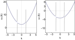
Figure 1: The variation of $\omega_{\pm}(k)$ with $k$ for $V_{0}=0$ (dashed blue line) and $V_{0}=-1$, $k_{l}=2$ (thick grey line). In both panel we take $\Omega_{0}=10$ and $k_{s}=2$. Here $\omega_{\pm}(k)$ and $k$ are measured in the units of $k_{s}^{2}$ and $k_{s}$ respectively.

Dynamical behavior of solution in the center of mass frame of the coupled system is described by Eq.(10). In analogy with $m\ddot{x}_{0}=-dV_{\rm eff}/dx_{0}$, Eq. (10) can be used to find the following effective potential for a particular time.

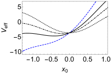
Figure 2: Effective potential of the center of mass of a soliton pairs for different values of initial phase $\varphi(0)=\pi/4$ (dashed curve, $\pi/8$(solid), $\pi/16$ (dot-dashed) and $0$ or $\pi$. Other parameters are fixed as: $k_{n}=1$, $V_{0}=-2$ and $\Gamma_{\gamma}=2.15$ and $\Gamma_{\beta}=0.35$, $Z(0)=0.5$ and $w=0.45$.

$$V_{\rm eff} = -\frac{N}{4w\sqrt{2\pi}}e^{-k_{n}^{2}w^{2}/2}\cos(2k_{n}x_{0})[\Gamma_{\gamma}+\Gamma_{\beta}Z^{2}]$$ (15)

$$+ V_{0}e^{-k_{l}^{2}w^{2}}\cos(2k_{l}x_{0})$$

$$- 2\Omega k_{s}\sqrt{1-Z^{2}}x_{0}e^{-k_{s}^{2}w^{2}}\sin(\varphi).$$

Understandably, $V_{\rm eff}$ describes effective potential that can cause the soliton to move(Fig.2). In absence of optical lattice the effective potential has no minimum. It develops local minima in presence of OLs. Depth of a local minimum increases with the decrease of initial phase difference $\varphi(0)$. We see that the effective potential becomes periodic with prominent local minima if $\varphi(0)$ is either $0$ or $\pi$( dotted curve). The nature of the effective potential sensitively depends on the soliton width ($w$) and lattice parameters. Thus one can control the motion of center of mass by taking appropriate lattice parameters.

IV JOSEPHSON-TYPE OSCILLATION BETWEEN TWO-WEAKLY COUPLED CONDENSATES

First we consider the case where center of mass of the system is located at a fixed position in the effective potential but the population imbalance occurs between the components due to interaction. For a fixed value of $x_{0}$, the coupled equations are reduced to the following pair of equations.

$$\frac{dZ}{dt}=-A\sqrt{1-Z^{2}}\sin(\varphi),$$ (16)

$$\frac{d\varphi}{dt} = (\Lambda+B)Z+\frac{AZ}{\sqrt{1-Z^{2}}}\cos(\varphi).$$ (17)

Here $A=2e^{-k_{s}^{2}w^{2}}\Omega(t)$ and $B=\frac{N\,\Gamma_{\beta}\,e^{\frac{-k_{n}^{2}w^{2}}{2}}}{\sqrt{2\pi}w}\cos(2k_{n}x_{0})$ with $\Gamma_{\beta}=(\gamma_{1}-\beta_{1})$. We see that the population imbalance parameter does not directly depend on the nonlinear lattice parameter but it may depend on lattice through the phase. However, the phase becomes independent of NOL if $\Gamma_{\beta}=0$. Therefore, the effects of lattice can be studied by taking appropriate values of $\Gamma_{\beta}$.

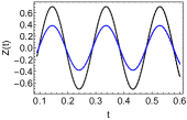
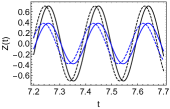
Figure 3: Left panel: Variation of atomic population imbalance ($Z(t)$) with $t$ for $\varphi(0)=\pi/8$(blue solid), $\varphi(0)=\pi/4$(black solid) in presence of optical lattices(OLs) while the dashed curves give the same in absence of OLs. Right Panel: It gives the plots similar to those used in the left panel near $t=7$. Other parameters are fixed as: $\gamma_{0}=2.5$, $\beta_{0}=2.25$, $\Gamma_{\beta}=-0.25$, $\Omega_{0}=20$, $k_{s}=1$, $x_{0}=0.25$, $w=0.45$ and $k_{n}=1$.

The variation of $Z$ with $t$ and its dependence on $\varphi$ is displayed in Fig.3. It is seen that the population imbalance oscillates with time (left panel). Amplitude of oscillation depends on the initial phase $\varphi(0)$. The period of oscillation is independent of $\varphi(0)$ (dashed curves). The oscillation of atomic population between two SOC states resembles with the concept of Josephson oscillation and thus we call it as Josephson-type (JT) oscillation. However, the period of oscillation is affected by the OLs (right panel, solid curve). Specifically, OLs imprint phases and thus causes the frequency of oscillation of population imbalance to increase. The frequency of oscillation obtained from Eq. (16) is given by[20]

$$\omega_{JT}=\left[A(\Lambda+B+\cos\varphi(0)A)\right]^{1/2}.$$ (18)

In writing Eq.(18) we have used $\ddot{Z}+\omega_{JT}^{2}Z=0$. The oscillation frequency depends on the initial value of $\varphi(t)$ and on the values of parameters $A$, $B$ and $\Lambda$ which vary with the lattice and SOC parameters. Particularly, $\omega_{JT}$ is maximum for $\varphi(0)=0$ while it is minimum for $\varphi(0)=\pi$. Variation of $\omega_{JT}$ with different $k_{s}$ (Fig. 4) indicates that oscillation frequencies for different $\varphi(0)$ values are distinguishable only in the limit of weak spin-orbit coupling.

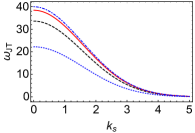
Figure 4: Frequency of JT oscillation for different values of initial phases $\varphi(0)=2\pi/5$ (blue dotted), $\pi/4$ (black dashed curve), $\pi/8$(red solid), and $0$ (blue dot-dashed). Other parameters are fixed as: $k_{n}=1$ and $\Gamma_{\gamma}=2.15$ and $\Gamma_{\beta}=0.35$, $Z(0)=0.5$ and $w=0.45$.

IV.1 Self-trapping of JT oscillation

For a fixed value of initial population imbalance ($z(0)$) and phase ($\varphi(0)$), the populations of the SOC states can be macroscopically quantum self-trapped (MQST) for a critical value of parameters. The MQST condition says that the total energy (Hamiltonian) $E=H[Z(t),\varphi(t)]$ of the system should satisfy the following condition[20, 28, 29]

$$H[Z(0),\varphi(0)]\!=\!\frac{1}{2}(\Lambda\!+\!B)Z(0)^{2}\!-\!A\cos(\varphi(0))\sqrt{1\!-\!Z(\!0)^{2}}\!\!>\!E_{-},$$ (19)

where $E_{-}$ is the value of $E$ at the stationary point $\varphi_{s}=(2n+1)\pi,\,\,Z_{s}=0$ of Eqs.(16) and (17). Clearly, $E_{-}=A$. One can check that the energy $(E)$ becomes $E_{+}=-A$ at $\varphi_{s}=2n\pi,\,\,Z_{s}=0$. In both the cases $Z-$symmetry remain valid. However, $z-$ symmetry breaks at the stationary point $\varphi_{s}=(2n+1)\pi,\,\,Z_{s}=\sqrt{1-A^{2}/(\Lambda+B)}$.

Let us define a parameter $\Theta_{c}$ at the critical point of MQST as follows.

$$\Theta_{c}=(\Lambda+B)/A.$$ (20)

Therefore, from Eq. (19) we can write

$$\Theta_{c}=\frac{2}{Z(0)^{2}}\left(1+\sqrt{1-Z(0)^{2}}\cos[\varphi(0)]\right).$$ (21)

This condition along with Eq. (20) allows us to find critical value of width($w_{c}$) for given values of different parameters of the system to get MQST. In Fig. 5, we plot $w_{c}$ with $\Gamma_{\beta}$ for different values of $k_{s}$. We see that critical value of width can be greater or smaller than that in the absence of the NOL (dotted vertical line, $\Gamma_{\beta}=0$). For particular values of lattice strengths, critical value of width decreases with the increase of $k_{s}$. The oscillation of population imbalance below and near the critical value of width is shown in the right panel of Fig. 5. It is seen that the time period of oscillation increases as we approach the critical width (red dotted curve). It becomes infinitely large if width exceed the critical value. Thus, it will not possible for the atoms to change states and they are trapped in their states (black dot-dashed curve).

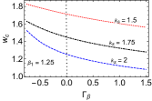
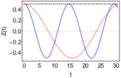
Figure 5: Left panel: Critical width ($w_{c}$) with different values of $\Gamma_{\beta}$ for self trapping. Here we have used $\beta_{0}=2.25$, $\gamma_{0}=2.5$, $k_{n}=1$, $\Omega_{0}=20$, $\varphi(0)=\pi$ and $Z(0)=0.5$. Right panel: $Z(t)$ versus $t$ with $k_{s}=1.5$ for $w=1.4$ (blue dashed line), $w=1.5$(red dotted line) and $w=1.66574$(black dot-dashed line).

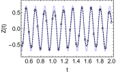
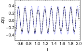
Figure 6: Left panel: Numerical results of JT oscillation in SOC BEC for $\varphi(0)=\pi/4$ in presence of nonlinear optical lattice with $\Gamma_{\beta}=1.15$, $\Gamma_{\gamma}=1.16$, $k_{n}=1$, $\gamma_{0}=2.5$, $\beta_{0}=2.25$, $k_{s}=1$, $w=0.45$, $\Omega_{0}=20$ and $x_{0}(0)=0.25$. Right panel: It shows JT oscillation for $\varphi(0)=\pi/8$ with the same values of parameters as used in the left panel. In both the panel black dots and solid blue curves represent the numerical and variational results respectively.

V Numerical simulation of JT oscillation

We have seen that population imbalance between spin-orbit coupled two condensates oscillates and oscillation is influenced by both SOC and lattice parameters using variational method. It is an approximation method. Therefore, it is quite essential to validate some of the obtained results through direct numerical simulation of GP equation in (3). In view of this, we use finite difference Crank-Nicholson scheme and achieve our goal using Thomas algorithm. Using Eq.(7) as initial density profile, we solve Eq. (7) and we plot $Z(t)$ with $t$ obtained from direct numerical simulation of GP equation (black big dots with dashed) and variational calculations in Fig. 6 for $\varphi(0)=\pi/4$(left panel) and $\varphi(0)=\pi/8$(right panel). Clearly, numerical results shows good agreement with the variational result(solid curve). We have also checked that $Z(t)$ versus $\varphi(t)$ describes a periodic motion.

Figure 7: Left panel: Variation of atomic population imbalance ($Z(t)$)in presence of both linear and nonlinear optical lattices for $V_{0}=-2$, $\varphi(0)=\pi/4$, $\Omega_{0}=20$, $k_{s}=1$, $\gamma_{0}=2.5$, $\beta_{0}=2.25$, $\Gamma_{\beta}=1.25$, $\Gamma_{\gamma}=1.26$ and $x_{0}=0.35$. We represent variational and numerical results by solid line and dashed line with big dots respectively. Right panel: Variation of $Z(t)$ with $\varphi(t)$ for different values of $t$.

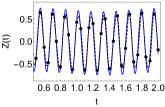
Figure 8: Numerical result of JT oscillation with time-dependent Rabi frequency and OLs for $\Omega_{0}=20$, $\Omega_{1}=0.2$, $\omega=32$, $\varphi(0)=\pi/4$, $\gamma_{0}=2.5$, $\beta_{0}=2.25$, $k_{s}=1$ , $\Gamma_{\beta}=1.25$, $\Gamma_{\gamma}=1.26$, $V_{0}=-2$, $k_{n}=k_{l}=1$ and $x_{0}=0.35$. Right panel: Variation of $Z(t)$ with $\varphi(t)$ for different values of $t$.

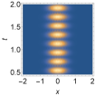
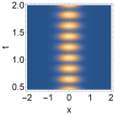
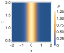
Figure 9: Density plots of the first component $\rho_{a}=|\psi_{a}|^{2}$ (left panel), second component $\rho_{b}=|\psi_{b}|^{2}$(middle panel) and total $\rho$(right panel) for $\Omega_{0}=20$ in presence of $\Gamma_{\beta}=1.25$, $\Gamma_{\gamma}=1.26$, $V_{0}=-2$, $k_{n}=k_{l}=1$, $\varphi(0)=\pi/4$, $\gamma_{0}=2.5$, $\beta_{0}=2.25$ and $k_{s}=1$.

We see that Eqs.(16) and (17) describing JT-oscillation do not involve the effects of linear optical lattice directly. However, one can fix initial width of matter-wave solitons using Eq.(11) from the stationary condition. Therefore, it is instructive to solve Eqs.(10)-(13) and compare the variational results with those obtained from numerical simulation. The result is displayed in Fig.7. We see that atomic population difference changes periodically with slightly different frequency and the variational result agrees the numerical result(left panel). The $\varphi$ dependence of $Z(t)$ (right panel) shows that the dynamical response of $Z(t)$ in OLs is not exactly periodic.

In all the above cases, we have considered that the Rabi frequency is constant. However, one can vary it with time as given in Eq.(7). The variation of JT oscillation with time-dependent frequency is shown in Fig.6. We see that the envelop of the population imbalance is periodically modified due to time-dependent Rabi frequency. Here we find the numerical result serves better than variational result.

It is an interesting curiosity to study density evolution of the spin-orbit coupled condensates during the change of population imbalance between the condensates in presence of OLs. The plots in Fig. 9 clearly shows that atomic densities of both the components(left and middle panels) change periodically but the changes are different for the two component at a particular time. For example, if the density of one component is maximum at time $t=t_{1}$ then the density of the other component is minimum at the same time $t_{1}$. However, the total density profile ($\rho$) remains constant with time (right panel).

VI conclusion

Bose-Einstein condensate serves an ideal platform to study different phenomena of condensed matter physics. Josephson oscillation is the one which can be realized in spin-orbit coupled Bose-Einstein condensates (SOC-BECs) through the oscillation of population imbalance between the coupled states. We consider Josephson-type oscillation in SOC-BECs with optical lattices and discuss its dependence on lattice and SOC parameters. More specifically, oscillation amplitude depends on the initial phase difference between components. Optical lattice changes phase velocity and thus increases the frequency of JT oscillation.

During the oscillation of the maximum value of population (MVP) both state are equal implying that average value of population imbalance is zero. However, it is also possible to create oscillation with unequal MVP in the SOC states. This is termed as quantum mechanical self-trapping(QMST). The QMST condition allows to determine critical value of width for the observation of self trapping. For given values of SOC parameters,lattice parameter can be used to control the value of critical parameter for QMST.

References

- [1] M. H. Anderson, J. R. Ensher, M. R. Matthews, C. E Wieman and E. A. Cornell, Observation of Bose–Einstein condensation in a dilute atomic vapor. Science 269, 198(1995).
- [2] C. C. Bradley, C. A.Sackett, J. J. Tollett and R. G. Hulet, Evidence of Bose–Einstein condensation in an atomic gas with attractive interactions. Phys. Rev. Lett. 75, 1687(1995).
- [3] Y. J. Lin, K. Jiménez-García and I. B. Spielman, Spin–orbit-coupled Bose-Einstein condensates, Nature 471, 83(2011).
- [4] Y. Zhang, M. E. Mossman, T. Busch, P. Engels, C. Zhang, Properties of spin-orbit-coupled Bose-Einstein condensates. Front. Phys. 11, 3(2016).
- [5] L. Khaykovich, F. Schreck, G. Ferrari, T. Bourdel, J. Cubizolles, L. D. Carr, Y. Castin, C. Salomon, Formation of a matter-wave bright soliton, Science 296, 1290(2002).
- [6] S. Burger, K. Bongs, S. Dettmer, W. Ertmer, and K. Sengstock, Dark solitons in Bose-Einstein condensates, Phys. Rev. Lett. 83, 25(1999).
- [7] O. Zobay, S. Pötting, P. Meystre, and E. M. Wright, Creation of gap solitons in Bose-Einstein condensates, Phys. Rev. A 59, 643(1999).
- [8] J. H. Denschlag, J. E. Simsarian, H. Häffner, C. McKenzie1, A. Browaeys, D. Cho, K. Helmerson, S. L. Rolston and W. D. Phillips, A Bose-Einstein condensate in an optical lattice, J. Phys. B: At. Mol. Opt. Phys. 35, 3095(2002).
- [9] M. Salerno, F. Kh. Abdullaev, A. Gammal, and L. Tomio, Tunable spin-orbit-coupled Bose-Einstein condensates in deep optical lattices, Phys. Rev. A 94, 043602(2016).
- [10] H. Sakaguchi and B. A. Malomed, Matter-wave solitons in nonlinear optical lattices, Phys. Rev. E 72, 046610 (2005).
- [11] G. A. Sekh, M. Salerno, A. Saha and B. Talukdar, Displaced dynamics of binary mixtures in linear and nonlinear optical lattices, Phys. Rev. A 85, 023639(2012). ).
- [12] Lin Wen, Q. Sun, Yu Chen, Deng-Shan Wang, J. Hu, H. Chen, W.-M. Liu, G. Juzeliunas, B. A. Malomed, and An-Chun Ji, Motion of solitons in one-dimensional spin-orbit-coupled Bose-Einstein condensates, Phys. Rev. A 94, 061602(R)(2016).
- [13] V. Achilleos, D. J .Frantzeskakis, P. G. Kevrekidis, D. E. Pelinovsky, Matter-wave bright solitons in spin-orbit coupled Bose-Einstein condensates, Phys. Rev. Lett. 110, 26(2013).
- [14] G. A. Sekh, B. Talukdar, S. Chatterjee and B. A. Khan, Information theoretic approach to effects of spin-orbit coupling in quasi-one-dimensional Bose-Einstein condensates, Phys. Scr. 97, 115404(2022).
- [15] L. Salasnich and B. A. Malomed, Localized modes in dense repulsive and attractive Bose-Einstein condensates with spin-orbit and Rabi couplings, Phys. Rev. A 87, 063625 (2013).
- [16] G. A. Sekh and B. Talukdar, Effects of optical lattices on bright solitons in spin-orbit coupled Bose-Einstein condensates, Phys. Lett. A, 415, 127665(2021).
- [17] M. Albiez, R. Gati, J. Folling, S. Hunsmann, M. Cristiani and M. K. Oberthaler, Direct observation of tunneling and nonlinear self-trapping in a single Bosonic Josephson junction, Phys. Rev. Lett. 95, 010402 (2005).
- [18] F. Kh. Abdullaev, M. Brtka, A. Gammal and L. Tomio, Solitons and Josephson-type oscillations in Bose-Einstein condensates with spin-orbit coupling and time-varying Raman frequency, Phys. Rev. A 97, 053611 (2018).
- [19] M. A. Garcia-March, G. Mazzarella, L. Dell‘Anna, B. Julia-Diaz, L. Salasnich, and A. Polls, Josephson physics of spin-orbit-coupled elongated Bose-Einstein condensates, Phys. Rev. A 89, 063607(2014).
- [20] S. Raghavan, A. Smerzi, S. Fantoni, and S. R. Shenoy, Coherent oscillations between two weakly coupled Bose-Einstein condensates: Josephson effects, oscillations, and macroscopic quantum self-trapping, Phys. Rev. A 59, 620(1999).
- [21] F. Kh Abdullaev, R. M. Galimzyanov and A. M. Shermakhmatov, Effects of quantum fluctuations on macroscopic quantum tunneling and self-trapping of a BEC in a double-well trap, J. Phys. B: At. Mol. Opt. Phys. 56, 165301(2023).
- [22] G. A. Sekh, F. V. Pepe, P. Facchi, S. Pascazio and M. Salerno, Split and overlapped binary solitons in optical lattices, Phys. Rev. A 92, 013639(2015).
- [23] Yaroslav V. Kartashov, Boris A. Malomed, and Lluis Torner, Solitons in nonlinear lattices, Rev. Mod. Phys. 83, 247(2011).
- [24] Yong Xu, Yongping Zhang, and Biao Wu, Bright solitons in spin-orbit-coupled Bose-Einstein condensates, Phys. Rev. A 87, 013614(2013).
- [25] R. Navarro, R. Carretero-Gonzàlez, and P. G. Kevrekidis, Phase separation and dynamics of two-component Bose-Einstein condensates, Phys. Rev. A 80, 023613(2009).
- [26] L. Wen, W. M. Liu, Yongyong Cai, J. M. Zhang, and Jiangping Hu, Controlling phase separation of a two-component Bose-Einstein condensate by confinement, Phys. Rev. A 85, 043602 (2012).
- [27] N. Ashcroft and N. David Mermin, Solid State Physics, 1st Edition, Harcourt Collage Publishers, 1976.
- [28] K. Rapedius, A heuristic approach to BEC self-trapping in double wells beyond the mean field, J. Phys. B: At. Mol. Opt. Phys. 45, 085303 (2012).
- [29] B. Cui, L. C. Wang, and X. X. Yi, Time-dependent self-trapping of Bose-Einstein condensates in a double-well potential, Phys. Rev. A 82, 062105(2010).