Tune-Mode ConvBN Blocks For Efficient Transfer Learning

Abstract

Convolution-BatchNorm (ConvBN) blocks are integral components in various computer vision tasks and other domains. A ConvBN block can operate in three modes: Train, Eval, and Deploy. While the Train mode is indispensable for training models from scratch, the Eval mode is suitable for transfer learning and model validation, and the Deploy mode is designed for the deployment of models. This paper focuses on the trade-off between stability and efficiency in ConvBN blocks: Deploy mode is efficient but suffers from training instability; Eval mode is widely used in transfer learning but lacks efficiency. To solve the dilemma, we theoretically reveal the reason behind the diminished training stability observed in the Deploy mode. Subsequently, we propose a novel Tune mode to bridge the gap between Eval mode and Deploy mode. The proposed Tune mode is as stable as Eval mode for transfer learning, and its computational efficiency closely matches that of the Deploy mode. Through extensive experiments in both object detection and classification tasks, carried out across various datasets and model architectures, we demonstrate that the proposed Tune mode does not hurt the original performance while significantly reducing GPU memory footprint and training time, thereby contributing an efficient solution to transfer learning with convolutional networks.

1 Introduction

Feature normalization (Huang et al., 2023) is a critical component in deep convolutional neural networks. Techniques such as batch normalization (Ioffe and Szegedy, 2015), group normalization (Wu and He, 2018), layer normalization (Ba et al., 2016), and instance normalization (Ulyanov et al., 2016) are designed to facilitate the training process by promoting stability, mitigating internal covariate shift, and enhancing network performance. Among these methods, batch normalization is arguably the most popular and widely adopted in computer vision tasks (Huang et al., 2023). A convolutional layer (LeCun et al., 1998) together with a consecutive BatchNorm layer is often called a ConvBN block, which operates in three modes:

• Train mode. Mini-batch statistics (mean and standard deviation $\mu,\sigma$) are computed for feature normalization, and running statistics ($\hat{\mu},\hat{\sigma}$) are tracked by exponential moving averages for testing individual examples when mini-batch statistics are unavailable.

• Eval mode. Running statistics are directly used for feature normalization without update, which is more efficient than Train mode, but requires tracked statistics to remain stable in training. It can also be used to validate models during development.

• Deploy mode. When the model does not require further training, computation in Eval mode can be accelerated (Markuš, 2018) by fusing convolution, normalization, and affine transformations into a single convolutional operator with transformed parameters. This is called Deploy mode, which produces the same output as Eval mode with better efficiency. In Deploy mode, parameters for the convolution are computed once-for-all, removing batch normalization for faster inference during deployment.

The three modes of ConvBN blocks present a trade-off between computational efficiency and training stability, as shown in Table 1. Train mode is applicable for both train from scratch and transfer learning, while Deploy mode optimizes computational efficiency. Consequently, these modes traditionally align with three stages in deep models’ lifecycle: Train mode for training, Eval mode for validation, and Deploy mode for deployment.

Table 1: Trade-off among modes of ConvBN blocks.

Mode	Train	Eval	Tune (proposed)	Deploy
Train From Scratch	✓	✗	✗	✗
Transfer Learning	✓	✓	✓	✗
Training Efficiency	$\star$	$\star$ $\star$	$\star$ $\star$ $\star$	$\star$ $\star$ $\star$

With the rise of transfer learning (Jiang et al., 2022), practitioners usually start with a pre-trained model, and instability of training from scratch is less of a concern. For instance, an object detector typically has one pre-trained backbone to extract features, and a head trained from scratch to predict bounding boxes and categories. Therefore, practitioners have started to explore Eval mode for transfer learning, which is more efficient than Train mode. Figure 1 presents the distribution of the normalization layers used in MMDetection (Chen et al., 2019), a popular object detection library. In the context of transfer learning, a majority of detectors (496 out of 634) are trained with ConvBN blocks in Eval mode. Interestingly, our findings suggest that Eval mode not only improves computational efficiency but also enhances the final performance over Train mode in certain transfer learning scenarios. For example, in Supplementary C, training Faster-RCNN (Ren et al., 2015) on COCO (Lin et al., 2014) with Eval mode achieves significantly better mAP than Train mode, with either pre-trained ResNet101 backbone or pre-trained HRNet backbone.

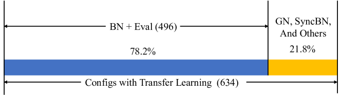
Figure 1: Distribution of normalization layer types used in all the 634 object detectors with pre-trained backbones in the MMDetection library (Chen et al., 2019). GN denotes GroupNorm, SyncBN represents synchronized BatchNorm across multiple GPUs and Eval indicates training ConvBN blocks in Eval mode. A majority of detectors (over 78%) are trained with ConvBN blocks in Eval mode.

Since transfer learning of ConvBN blocks in Eval mode has been a common practice, and forward calculation results between Deploy mode and Eval mode are equivalent, it is natural to ask if we can use Deploy mode for more efficient training. Unfortunately, direct training in Deploy mode can lead to instability, as demonstrated in Section 3.3.

In quest of efficient transfer learning from pre-trained models with ConvBN blocks, we theoretically uncover the underlying causes of training instability in Deploy mode and subsequently propose a novel Tune mode. It bridges the gap between Eval mode and Deploy mode, preserving functional equivalence with Eval mode in both forward and backward propagation while approaching the computational efficiency of Deploy mode. Our extensive experiments across several tasks (object detection and classification), model architectures, and datasets confirm the significant reduction in memory footprint and wall-clock training time without sacrificing performance.

2 Related Work

2.1 Normalization Layers

Feature normalization has long been established in machine learning (Bishop, 2006), e.g., Z-score normalization to standardize input features for smooth and isotropic optimization landscapes (Boyd and Vandenberghe, 2004). With the emergence of deep learning, normalization methods specifically tailored to intermediate activations, or feature maps, have been developed and gained traction.

Batch normalization (BN), proposed by Ioffe and Szegedy (2015), demonstrated that normalizing intermediate layer activations could expedite training and mitigate the effects of internal covariate shift. Since then, various normalization techniques have been proposed to address specific needs, such as group normalization (Wu and He, 2018) for small batch sizes, and layer normalization (Ba et al., 2016) typically employed in natural language processing tasks. We direct interested readers to the survey by Huang et al. (2023) for an in-depth exploration of normalization layers.

Among various types of normalization, BatchNorm is arguably the most prevalent choice for convolutional neural networks (CNNs), partly due to its ability to be fused within convolution operations during deployment. This fusion allows ConvBN blocks to be efficiently deployed to a wide variety of devices. Conversely, other normalization layers exhibit different behaviors compared to BatchNorm and often entail higher computational costs during deployment. In this paper, we focus on ConvBN blocks with convolution and BatchNorm layers in transfer learning, aiming to enhance training efficiency in terms of both memory footprint and computation time.

2.2 Variants of Batch Normalization

While batch normalization successfully improves training stability and convergence, it presents several limitations. These limitations originate from the different behavior during training and validation (Train mode and Eval mode), which is referred to as train-inference mismatch (Gupta et al., 2019) in the literature. Ioffe (2017) proposed batch renormalization to address the normalization issues with small batch sizes. Wang et al. (2019) introduced TransNorm to tackle the normalization problem when adapting a model to a new domain. Recently, researchers find that train-inference mismatch of BatchNorm plays a critical role in test-time domain adaptation (Wang et al., 2021, 2022). In this paper, we focus on the Eval mode of ConvBN blocks, which is free of train-inference mismatch because of its consistent behavior during both training and inference.

Another challenge posed by BatchNorm is its memory intensiveness. While the computation of BatchNorm is relatively light compared with convolution, it occupies nearly the same memory as convolution because it records the feature map of convolutional output for back-propagation. To address this issue, Bulo et al. (2018) proposed to replace the activation function (ReLU (Nair and Hinton, 2010)) following BatchNorm with an invertible activation (such as Leaky ReLU (Maas et al., 2013)), thereby eliminating the need to store the output of convolution for backpropagation. However, this approach imposes an additional computational burden on backpropagation, as the input of activations must be recomputed by inverting the activation function. Their reduced memory footprint comes with the price of increased running time. In contrast, our proposed Tune mode effectively reduces both computation time and memory footprint for efficient transfer learning without any modification of network activations or any other architecture.

2.3 Transfer Learning

Training deep neural networks used to be difficult and time-consuming. Fortunately, with the advent of advanced network architectures like skip connections (He et al., 2016), and the availability of foundation models (Bommasani et al., 2022), practitioners can now start with pre-trained models and fine-tune them for various applications. Pre-trained models offer general representations (Donahue et al., 2014) that can accelerate the convergence of fine-tuning in downstream tasks. Consequently, the rule of thumb in computer vision tasks is to start with models pre-trained on large-scale datasets like ImageNet (Deng et al., 2009), Places (Zhou et al., 2018), or OpenImages (Kuznetsova et al., 2018). This transfer learning paradigm alleviates the data collection burden required to build a deep model with satisfactory performance and can also expedite training, even if the downstream task has abundant data (Mahajan et al., 2018).

Train mode is the only mode for training ConvBN blocks from scratch. However, it is possible to use Eval mode for transfer learning, as we can exploit pre-trained statistics without updating them. Moreover, Eval mode is more computationally efficient than Train mode. Consequently, researchers usually fine-tune pre-trained models in Eval mode (Chen et al., 2019) (Figure 1), which maintains performance while offering improved computational efficiency. In this paper, we propose a novel Tune mode that further reduces memory footprint and training time while maintaining functional equivalence with the Eval mode during both forward and backward propagation, leading to an efficient solution for transfer learning with ConvBN blocks.

2.4 Training-Time Computation Graph Modification

PyTorch (Paszke et al., 2019), a widely adopted deep learning framework, uses dynamic computation graphs, wherein the graph is built on-the-fly with computation. This imperative style of computation is user-friendly, which contributed to PyTorch’s rapid rise in popularity. Nevertheless, the dynamic computation graphs complicate the speed optimization. Traditionally, operator analysis and fusion were only applied to models after training. The speed optimization usually involved a separate language or framework such as TensorRT (Vanholder, 2016) or other domain-specific languages, distinct from the Python language commonly employed for training. Recently, PyTorch’s built-in package torch.fx (Reed et al., 2022) exposes the computation graph to users in an accessible manner by a minimized set of primitive operations, which facilitates the manipulation of computation graph for a broad range of models in Python during training. Thanks to torch.fx, our proposed Tune mode can automatically identify consecutive Convolution and BatchNorm layers without manual intervention. Consequently, switching to Tune mode is as simple as a one-line code change, as described in Section 4.

3 Method

3.1 Problem Setup

In this paper, we study ConvBN blocks, which are prevalent in various computer vision tasks and other domains. A ConvBN block consists of two layers: (1) a convolutional layer with parameters of weight $\omega$ and bias $b$; (2) a BatchNorm layer with tracked mean $\hat{\mu}$ and standard deviation $\hat{\sigma}$, and trainable parameters weight $\gamma$ and bias $\beta$. We focus on the inner calculation of ConvBN blocks, which is not affected by activation functions or skip connections after ConvBN blocks.

Given an input tensor $X$ with dimensions $[N,C_{\text{in}},H_{\text{in}},W_{\text{in}}]$, where $N$ represents the batch size, $C_{\text{in}}$ the number of input channels, and $H_{\text{in}}/W_{\text{in}}$ the spatial height/width of the input, the ConvBN block in Eval mode (the majority choice in transfer learning as shown in Figure 1) operates as follows. First, the convolutional layer computes an intermediate output tensor $Y=\omega\circledast X+b$ (we use $\circledast$ to denote convolution), resulting in dimensions $[N,C_{\text{out}},H_{\text{out}},W_{\text{out}}]$. Subsequently, the BN layer normalizes and applies an affine transformation to the intermediate output, producing the final output tensor $Z=\gamma\frac{Y-\hat{\mu}}{\sqrt{\hat{\sigma}^{2}+\varepsilon}}+\beta$ with the same dimensions as $Y$.

Usually, the training loss consists of two parts: $J=J(Z)$ calculated on the network’s output, and regularization loss $R$ calculated on the network’s trainable parameters. Training is dominated by the gradient from $J(Z)$, especially at the beginning of training. The influence of $R$ is rather straightforward to analyze, since it directly and independently applies to each parameter. We omit the analysis for simplicity, as it does not change the main conclusion of this paper. Therefore, our primary focus lies in understanding the gradient with respect to the output loss function $J(Z)$ under different modes of ConvBN blocks. Note that $J(Z)$ can represent loss directly calculated on $Z$, and loss computed based on the output of subsequent layers operating on $Z$.

3.2 Preliminary

Backward Propagation of Convolution: To discuss the stability of training, we must examine the details of backward propagation to understand the behavior of the gradient for each parameter. For a convolution layer with forward computation $Y=\omega\circledast X+b$, if the gradient back-propagated to $Y$ is $\frac{\partial{J}}{\partial{Y}}$, then the gradients of each input of the convolution layer (as explained in (Bouvrie, 2006)) are: $\frac{\partial{J}}{\partial{\omega}}=\frac{\partial{J}}{\partial{Y}}\odot X;\frac{\partial{J}}{\partial{X}}=\omega_{\text{rot}}\circledast\frac{\partial{J}}{\partial{Y}};\frac{\partial{J}}{\partial{b}}=\frac{\partial{J}}{\partial{Y}}$. The $\odot$ represents cross-correlation, and $\omega_{\text{rot}}$ is the rotated version of $\omega$, both are used to compute the gradient of convolution (Rabiner and Gold, 1975).

Associative Law for Convolution and Affine Transform: Convolution can essentially be viewed as a patch-wise matrix-vector multiplication, with the matrix (kernel weight) having a shape of $[C_{\text{out}},k^{2}C_{\text{in}}]$, and the vector having a shape of $[k^{2}C_{\text{in}}]$. If an affine transform is applied to the weight along the $C_{\text{out}}$ dimension, then the affine transform is associative with the convolution operator. Formally speaking, $\gamma\cdot(\omega\circledast X)=(\gamma\cdot\omega)\circledast X$, where $\gamma$ is a $C_{\text{out}}$-dimensional vector multiplied to each row of the weight $\omega$. This association law lays the foundation of analyses for the Deploy mode and our proposed Tune mode.

Backward Propagation of Broadcast: Modern array/tensor libraries like NumPy (Harris et al., 2020) and PyTorch (Paszke et al., 2019) heavily rely on broadcasting, a technique to allow element-wise arithmetic between two tensors with different shapes. We adopt this notation and clarify any potential confusion here. For instance, the convolutional output $Y$ has a shape of $[N,C_{\text{out}},H_{\text{out}},W_{\text{out}}]$, while the tracked mean $\hat{\mu}$ has a shape of $[C_{\text{out}}]$, and $Y-\hat{\mu}$ implies first replicating $\hat{\mu}$ to have a shape of $[N,C_{\text{out}},H_{\text{out}},W_{\text{out}}]$, then performing element-wise subtraction. This can be explained by introducing an additional broadcast operator $\mathcal{B}_{Y}$, where $\mathcal{B}_{Y}(\hat{\mu})$ broadcasts $\hat{\mu}$ to match the shape of $Y$. The underlying calculation is actually $Y-\mathcal{B}_{Y}(\hat{\mu})$. The backward calculation for the broadcast operator $\frac{\partial{\mathcal{B}_{Y}(\hat{\mu})}}{\partial{\hat{\mu}}}$ is the reverse of replication, i.e., summing over a large tensor with the shape of $[N,C_{\text{out}},H_{\text{out}},W_{\text{out}}]$ into a smaller tensor with the shape of $[C_{\text{out}}]$. This helps understand the backward equation for the bias term $\frac{\partial{J}}{\partial{b}}=\frac{\partial{J}}{\partial{Y}}$, which actually means $\frac{\partial{J}}{\partial{b}}=\frac{\partial{\mathcal{B}_{Y}(b)}}{\partial{b}}\frac{\partial{J}}{\partial{Y}}$, i.e., summing $\frac{\partial{J}}{\partial{Y}}$ to be compatible with the shape of $\frac{\partial{J}}{\partial{b}}$. Due to the prevalence of broadcast in neural networks, we omit them to simplify equations. In this paper, any shape mismatch in equations should be resolved by taking broadcast (backward or forward) into account.

Table 2: Computation graph of ConvBN blocks in different modes. Shape annotations for each tensor are available in Supplementary A. Our proposed Tune mode bridges the gap between Eval mode and Deploy mode, alleviating the dilemma between training stability and computational efficiency.

Mode	Computation Graph	Backward Propagation
Eval		$\small\begin{aligned} &\frac{\partial J}{\partial X}=\frac{\gamma}{\sqrt{\hat{\sigma}^{2}+\epsilon}}\omega_{\text{rot}}\circledast\frac{\partial J}{\partial Z}\\[5.69054pt] &\frac{\partial J}{\partial\omega}=\frac{\gamma}{\sqrt{\hat{\sigma}^{2}+\epsilon}}\frac{\partial{J}}{\partial{Z}}\odot X\\[5.69054pt] &\frac{\partial{J}}{\partial{b}}=\frac{\gamma}{\sqrt{\hat{\sigma}^{2}+\epsilon}}\frac{\partial{J}}{\partial{Z}}\\[5.69054pt] &\frac{\partial{J}}{\partial{\gamma}}=\frac{\partial{J}}{\partial{Z}}\frac{Y-\hat{\mu}}{\sqrt{\hat{\sigma}^{2}+\epsilon}}\\[5.69054pt] &\frac{\partial{J}}{\partial{\beta}}=\frac{\partial{J}}{\partial{Z}}\end{aligned}$
Tune (Proposed)		$\small\begin{aligned} &\frac{\partial{J}}{\partial{X}}=\omega_{\text{rot}}^{\prime}\circledast\frac{\partial{J}}{\partial{Z}}\\[5.69054pt] &\frac{\partial{J}}{\partial{\omega^{\prime}}}=\frac{\partial{J}}{\partial{Z}}\odot X\\[5.69054pt] &\frac{\partial{J}}{\partial{\omega}}=\frac{\gamma}{\sqrt{\hat{\sigma}^{2}+\epsilon}}\frac{\partial{J}}{\partial{\omega^{\prime}}}\\[5.69054pt] &\frac{\partial{J}}{\partial{b}}=\frac{\gamma}{\sqrt{\hat{\sigma}^{2}+\epsilon}}\frac{\partial{J}}{\partial{Z}}\\[5.69054pt] &\frac{\partial{J}}{\partial{\gamma}}=\frac{\partial{J}}{\partial{\omega^{\prime}}}\frac{\omega}{\sqrt{\hat{\sigma}^{2}+\epsilon}}+\frac{\partial{J}}{\partial{Z}}\frac{b-\hat{\mu}}{\sqrt{\hat{\sigma}^{2}+\epsilon}}\\[5.69054pt] &\frac{\partial{J}}{\partial{\beta}}=\frac{\partial{J}}{\partial{Z}}\end{aligned}$
Deploy		$\small\begin{aligned} &\frac{\partial{J}}{\partial{X}}=\omega_{\text{rot}}^{\prime}\circledast\frac{\partial{J}}{\partial{Z}}\\[5.69054pt] &\frac{\partial{J}}{\partial{\omega^{\prime}}}=\frac{\partial{J}}{\partial{Z}}\odot X\\[5.69054pt] &\frac{\partial{J}}{\partial{b^{\prime}}}=\frac{\partial{J}}{\partial{Z}}\end{aligned}$

With the necessary background established, we directly present the forward, backward, and memory footprint details in Table 2. Note that intermediate tensors saved for back-propagation can be identified by back-propagation equations: variables (to be specific, $X,Y$ in Eval mode, $X,\omega^{\prime},b^{\prime}$ in Tune mode, and $X$ in Deploy mode) other than the gradient should be saved during forward calculation. Further analyses will be provided in subsequent sections.

3.3 Analyzing Eval Mode and Deploy Mode

With the help of equations in Table 2, the comparison between Eval mode and Deploy mode on efficiency and training stability is as straightforward as follows.

3.3.1 Forward Computation Efficiency

We first observe that Eval mode and Deploy mode have equivalent results in forward computation, and Deploy mode is more efficient. The equivalence can be proved by the definitions $\omega^{\prime}=\frac{\gamma}{\sqrt{\hat{\sigma}^{2}+\epsilon}}\cdot\omega$ and $b^{\prime}=\left(b-\hat{\mu}\right)\frac{\gamma}{\sqrt{\hat{\sigma}^{2}+\epsilon}}+\beta$, together with the associative law for convolution and affine transformations. However, Deploy mode pre-computes the weight $\omega^{\prime}$ and $b^{\prime}$, reducing the forward propagation to a single convolution calculation. Conversely, Eval mode requires a convolution, supplemented by a normalization and an affine transform on the convolutional output. This results in a slower forward propagation process for Eval mode. Moreover, Eval mode requires storing $X,Y$ for backward propagation, while Deploy mode only stores $X$. The memory footprint of Eval mode is nearly double of that in Deploy mode. Therefore, Deploy mode emerges as the more efficient of the two in terms of memory usage and computational time.

3.3.2 Training Stability

Our analyses suggest that Deploy mode tends to exhibit less training stability than Eval mode. Focusing on the convolutional weight, which constitutes the primary parameters in ConvBN blocks, we observe from Table 2 that the relationship of values and gradients between Deploy mode and Eval mode is $\omega^{\prime}=\frac{\gamma}{\sqrt{\hat{\sigma}^{2}+\epsilon}}\omega$ and $\frac{\partial J}{\partial\omega^{\prime}}=\frac{\sqrt{\hat{\sigma}^{2}+\epsilon}}{\gamma}\frac{\partial J}{\partial\omega}$. The scaling coefficients of the weight ($\frac{\gamma}{\sqrt{\hat{\sigma}^{2}+\epsilon}}$) are inverse of the scaling coefficients of the gradient ($\frac{\sqrt{\hat{\sigma}^{2}+\epsilon}}{\gamma}$). This can potentially cause training instability in Deploy mode. For instance, if $\frac{\gamma}{\sqrt{\tilde{\sigma}^{2}+\epsilon}}$ is small (say $0.1$), the weight reduces to one-tenth of its original value, while the gradient increases tenfold. This is a significant concern in real-world applications. As illustrated in Figure 2, these scaling coefficients can range from as low as $0$ to as high as $30$, leading to unstable training. Figure 2 further substantiates this point through end-to-end experiments in both object detection and classification using Eval mode and Deploy mode. Training performance in Deploy mode is markedly inferior to that in Eval mode.

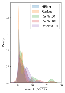
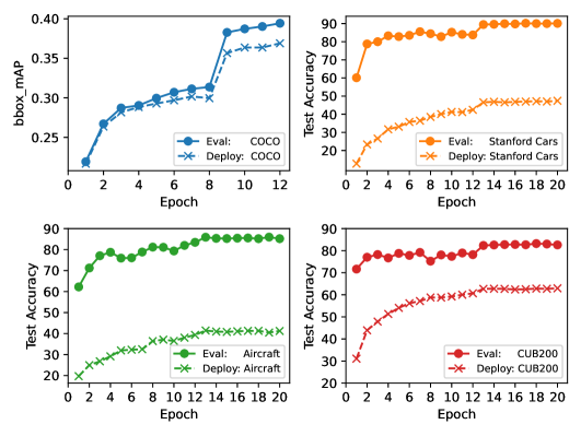
Figure 2: (a): Distribution of scaling coefficients for weight $\left(\gamma/\sqrt{\hat{\sigma}^{2}+\epsilon}\right)$ in different backbones. (b): Comparison between training with Eval mode and Deploy mode in both object detection and classification. Severe performance degradation is observed for training with Deploy mode.

In conclusion, Deploy mode and Eval mode share the same forward calculation results, but present a dilemma in computation efficiency and training stability.

3.4 Tune Mode v.s. Deploy Mode and Eval Mode

Table 2 describes the detailed computation of the proposed Tune mode specifically designed for efficient transfer learning. This mode leverages the associative law of convolution and affine transformation, optimizing both memory and computation. The main point is to calculate the transformed parameters dynamically, on-the-fly. Next, we provide two critical analyses to show how the proposed Tune mode addresses the dilemma between training stability and computational efficiency, and how it bridges the gap between Eval mode and Deploy mode.

3.4.1 Training Stability

The associative law between convolution and affine transformation readily implies that the forward calculations between Eval mode and Tune mode are equivalent. The equivalence of backward calculations is less intuitive, particularly when considering the gradient relating to $\gamma$. To validate this, we employ an alternative approach: let $Z_{1},Z_{2}$ represent the outputs of Eval mode and Tune mode, respectively. We define $Z_{1}=Z_{1}(\omega,b,\gamma,\beta),Z_{2}=Z_{2}(\omega,b,\gamma,\beta)$. Given that $Z_{1}=Z_{2}$, and both are functions computed from the same set of parameters ($\omega,b,\gamma,\beta$), we can assert that their Jacobian matrices coincide: $\frac{\partial{Z_{1}}}{\partial{[\omega,b,\gamma,\beta]}}=\frac{\partial{Z_{2}}}{\partial{[\omega,b,\gamma,\beta]}}$. This immediately suggests that both modes share the same backward propagation dynamics. Consequently, we can conclude that Tune mode is as stable as Eval mode in transfer learning. They are equivalent up to the error of floating point calculation (e.g., $0.1\times(0.3\times 0.7)-(0.1\times 0.3)\times 0.7\approx 3\times 10^{-18}$ in 64-bit floating point calculation).

3.4.2 Efficiency

Computation in Eval mode consists of a convolution followed by an affine transformation on the convolutional feature map $Y$. Conversely, Tune mode computation consists of an affine transformation on the original convolutional weights $\omega$ succeeded by a convolution with the transformed weights $\omega^{\prime}$. Since feature maps $Y$ are usually larger than convolutional weights $\omega$, an affine transformation on convolutional weights executes faster than on feature maps. Concerning memory usage for backpropagation, Eval mode requires saving the input feature map $X$ and the convolutional output $Y$. In contrast, Tune mode stores $X$ and the transformed weights $\omega^{\prime}$. This difference signifies that Tune mode requires less memory for transfer learning. Therefore, Tune mode outperforms Eval mode both in memory usage and computation speed. We assess memory usage and computation time for one-iteration of fine-tuning using a standard ResNet-50 (He et al., 2016) model with variable batch sizes and input sizes. The results, displayed in Figure 3, clearly indicate that Tune mode is more efficient than Eval mode across all tested settings. The memory footprint of Tune mode consumed by pre-trained backbone in transfer learning can be reduced to one half of that in Eval mode, and the computation time is reduced by about $10\%$. The comparison between Tune and Deploy in efficiency can be found in Supplementary E, they are nearly the same in terms of efficiency, and therefore we omit the comparison in the main text to keep the plot clear.

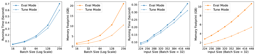
Figure 3: Memory footprint and running time comparison for Eval mode and Tune mode. The base setting is batchsize $=32$ and input dimension $=224\times 224$, and we vary batchsize and input dimension to test the efficiency.

The comparison among Eval/Tune/Deploy can be summarized as follows:

• $\text{Deploy mode}\approx\text{Tune mode}>\text{Eval mode}$, in terms of efficiency.

• $\text{Eval mode}=\text{Tune mode}>\text{Deploy mode}$, in terms of training stability.

Therefore, the proposed Tune mode successfully bridges the gap between Eval mode and Tune mode, improving the efficiency of transfer learning with Eval mode while keeping the stability of training.

4 Experiments

We use torch.fx to programmatically find consecutive convolution and BatchNorm layers. To use the proposed Tune mode, users just need to add one line of code turn_on(model, mode=‘‘Tune’’) in PyTorch (Paszke et al., 2019). Code details can be found in Supplementary B. Our main results are reported in two transfer learning tasks (object detection and object classification). We also show that Tune mode can be used in pre-training in Supplementary I.

For all the experiments, we first follow official guidelines from their open-source libraries (namely MMDetection, TLlib, and PyTorch ImageNet pre-training) to obtain baseline results. Then we add one line to turn on Tune mode for these models, and record the performance, computation time, and memory footprint to calculate the benefit of Tune mode. Hyper-parameters are taken from libraries’ default values to ensure a fair comparison. The proposed Tune mode has no hyper-parameters.

The total computation for results reported in this paper is about $3400$ hours of V100 GPU (32GB), as recorded by internal computing infrastructure. Supplementary H gives more details on this estimation.

4.1 Object Classification

We first use Tune mode for the popular open-source TLlib (Jiang et al., 2022), which includes widely used datasets for transfer learning benchmarks. The datasets include CUB-200 (Wah et al., 2011) for fine-grained bird classification, Standford Cars (Krause et al., 2013) and Aircrafts (Maji et al., 2013). The backbone for transfer learning is ResNet50 pre-trained on ImageNet. Each experiment is repeated three times with different random seeds to report mean and standard deviation, and the original data before averaging can be found in Supplementary D. Results are reported in Table 3.

Note that TLlib uses Train mode by default, and we find that switching to the proposed Tune mode does not hurt performance (actually we observe a slight increase in performance). The Tune mode reduces over $10\%$ computation time and about $40\%$ memory footprint.

Table 3: Results for Tune mode in classification using TLlib.

Dataset	mode	Accuracy	Memory (GB)	Time (second/iteration)
CUB-200	Train	83.07 ($\pm$ 0.15)	19.967	0.571
	Tune	83.20 ($\pm$ 0.00)	12.323 (38.28%$\downarrow$)	0.501 (12.26%$\downarrow$)
Aircrafts	Train	85.40 ($\pm$ 0.20)	19.965	0.564
	Tune	85.90 ($\pm$ 0.26)	12.321 (38.28%$\downarrow$)	0.505 (10.51%$\downarrow$)
Stanford Cars	Train	89.87 ($\pm$ 0.06)	19.967	0.571
	Tune	90.13 ($\pm$ 0.12)	12.321 (38.28%$\downarrow$)	0.491 (14.00%$\downarrow$)

4.2 Object Detection

This section presents object detection results on the widely used COCO (Lin et al., 2014) dataset. The MMDetection library uses Eval mode by default, and we compare the results by switching models to Tune mode. We test against various mainstream CNN backbones, including ResNet (He et al., 2016), ResNext (Xie et al., 2017), RegNet (Radosavovic et al., 2020), and HRNet (Wang et al., 2020). Results are shown in Table 4, with links for each config file for reference.

Note that detection models typically have a pre-trained backbone for extracting features, and a head trained from scratch for producing bounding boxes and classification. The head consumes the major computation time. Our Tune mode can only be used for backbone, since it is the only part using transfer learning. Therefore, computation speedup is not obvious in objection detection, and we only report the reduction of memory footprint here.

Object detection experiments are costly, and therefore we do not repeat three times to calculate mean and standard deviation. Supplementary G shows that the standard deviation of performance across different runs is as small as $0.0005$. The change of mAP in Table 4 can be attributed to randomness across experiments.

With different architecture, batch size and training precision (Micikevicius et al., 2018), Tune mode has almost the same mAP as Eval mode, while remarkably reducing the memory footprint by about $20\%\sim 40\%$.

Table 4: Object Detection results. Each detector is linked to detailed configuration files for reference.

Detector	Backbone	BatchSize	Precision	mode	mAP	Memory(GB)
Faster RCNN	ResNet50	2	FP32	Eval	0.3739	3.857
				Tune	0.3728 (-0.0011)	3.003 (22.15%$\downarrow$)
Mask RCNN	ResNet50	2	FP32	Eval	0.3824	4.329
				Tune	0.3825 (+0.0001)	3.470 (19.85%$\downarrow$)
Mask RCNN	ResNet101	16	FP16	Eval	0.3755	13.687
				Tune	0.3756 (+0.0001)	9.980 (27.08%$\downarrow$)
Retina Net	ResNet50	2	FP32	Eval	0.3675	3.631
				Tune	0.3647 (-0.0028)	2.774 (23.59%$\downarrow$)
Faster RCNN	ResNet101	2	FP32	Eval	0.3944	5.781
				Tune	0.3921 (-0.0023)	4.183 (27.65%$\downarrow$)
Faster RCNN	ResNet101	2	FP16	Eval	0.3944	3.849
				Tune	0.3925 (-0.0019)	3.138 (18.47%$\downarrow$)
Faster RCNN	ResNet101	8	FP16	Eval	0.3922	10.411
				Tune	0.3917 (-0.0005)	7.036 (32.41%$\downarrow$)
Faster RCNN	ResNet101	16	FP16	Eval	0.3902	19.799
				Tune	0.3899 (-0.0003)	12.901(34.83%$\downarrow$)
Faster RCNN	ResNext101	2	FP32	Eval	0.4126	6.980
				Tune	0.4131 (+0.0005)	4.773 (31.62%$\downarrow$)
Faster RCNN	RegNet	2	FP32	Eval	0.3985	4.361
				Tune	0.3995 (+0.0010)	3.138 (28.06%$\downarrow$)
Faster RCNN	HRNet	2	FP32	Eval	0.4017	8.504
				Tune	0.4031 (+0.0014)	5.463 (35.76%$\downarrow$)

4.3 Comparing to Other Memory Reduction Method

We compare our proposed Tune Mode with the Inplace-ABN (Bulo et al., 2018), a memory reduction method for ConvBN blocks by invertible activations. We show transfer learning experiments on the Aircraft dataset with the same settings of section 4.1, and the full experiments on all three datasets can be found in Supplementary F.

To apply Inplace-ABN blocks, we find BN-ReLU patterns in the pretrained network using torch.fx and replace them with the Inplace-ABN blocks provided by Bulo et al. (2018). Results are summarized in Table LABEL:tbl:inplace_abn. Inplace-ABN block saves approximately 16% memory at the cost of $8\%$ computation time, and also hurts the accuracy significantly as it modifies the network architecture. Compared to Inplace-ABN, our proposed Tune mode saves more memory footprint and requires less computation time, while retaining the accuracy.

Table 5: Comparision between proposed Tune Mode and the Inplace-ABN (Bulo et al., 2018).

	Accuracy	Memory (GB)	Time (second/iteration)
Baseline	85.40 ($\pm$0.20)	19.965	0.564
Inplace-ABN	78.23 ($\pm$0.45)	16.737 (16.17%$\downarrow$)	0.620 (8.58%$\uparrow$)
Tune Mode (ours)	85.90 ($\pm$0.26)	12.323 (38.28%$\downarrow$)	0.505 (10.51%$\downarrow$)

5 Conclusion

This paper proposes a new Tune mode for ConvBN blocks as a drop-in enhancement to achieve efficient transfer learning. Tune Mode is equivalent to Eval mode in both forward and backward calculation and reduces memory footprint and computation time without hurting performance. Our experiments show that Tune Mode performs well in transfer learning scenarios including object detection and fine-grained image classification. With one-line code change, Tune mode can save at most $38\%$ memory and $14\%$ computation time. Broader impact and limitations are discussed in Supplementary J.

Supplementary Material
“Tune-Mode ConvBN Blocks For Efficient Transfer Learning”

Appendix A Code Details of Train/Eval/Deploy Mode

Cmputation details of ConvBN blocks in different modes, with shape annotations for each tensor available in the following code snippet.

⬇

1# input: A faeture map $X$. The shape of $X$ is $[N,C_{in},H_{in},W_{in}]$.

2# input: A convolutional layer "conv" with kernel-size $k$ and output channel number $C_{out}$; it has a weight parameter $W$ with the shape of $[C_{out},C_{in},k,k]$ and a bias parameter $b$ with the shape of $[C_{out}]$.

3# input: A BatchNorm layer "bn" with output channel number $C_{out}$; it has a weight parameter $\gamma$ with the shape of $[C_{out}]$, and a weight parameter $\beta$ with the shape of $[C_{out}]$. The momentum update rate of BatchNorm is a constant number $\alpha\in(0,1)$.

4# output: Z = bn(conv(X))

5

6# code explained in a pytorch style

7import torch

8

9"Train Mode"

10# calculate the output of convolution

11$Y$ = $W\circledast\ X+b$ # $\circledast$ for convolution. The shape of $Y$ is $[N,C_{out},H_{out},W_{out}]$

12# calculate the mean for normalization

13$\mu$ = torch.mean($Y$, dim=(0, 2, 3)) # $\mu$ has a shape of $[C_{out}]$

14# calculate the variation for normalization

15$\sigma^{2}$ = torch.var($Y$, dim=(0, 2, 3)) # $\sigma^{2}$ has a shape of $[C_{out}]$

16# update tracked statistics, $\hat{\mu}$ and $\hat{\sigma^{2}}$ keep track of moving mean and moving variance. They are initialized to 0 and 1 respectively if the model is trained from scratch, or are inherited from pre-trained values.

17$\hat{\mu}\leftarrow\hat{\mu}+\alpha(\mu-\hat{\mu})$

18$\hat{\sigma}^{2}\leftarrow\hat{\sigma}^{2}+\alpha(\sigma^{2}-\hat{\sigma}^{2})$

19

20# normalize the output

21# $\epsilon$ is a small positive number to avoid zero division

22$\bar{Y}=\frac{Y-\mu}{\sqrt{\sigma^{2}+\epsilon}}$ # $\mu$ and $\sigma^{2}$ are broadcast to match the shape of $Y$

23# apply the affine transform

24$Z=\gamma*\bar{Y}+\beta$ # $\gamma$ and $\beta$ are broadcast to match the shape of $\bar{Y}$

25

26"Eval Mode"

27# calculate the output of convolution

28$Y$ = $W\circledast X+b$

29# normalize the output with tracked statistics

30$\bar{Y}=\frac{Y-\hat{\mu}}{\sqrt{\hat{\sigma^{2}}+\epsilon}}$

31# apply the affine transform

32$Z=\gamma*\bar{Y}+\beta$

33

34"Deploy Mode"

35# update the weight and bias of the convolution once for all

36$\hat{W}=W*\frac{\gamma}{\sqrt{\hat{\sigma}^{2}+\epsilon}}$

37$\hat{b}=(b-\hat{\mu})\frac{\gamma}{\sqrt{\hat{\sigma}^{2}+\epsilon}}+\beta$

38

39# convolution with updated parameters is equivalent to consecutive convolution and batch normalization

40$Z$ = $\hat{W}\circledast X+\hat{b}$

Listing 1: Computation details for consecutive Convolution and BatchNorm layers in different modes

Appendix B Code Details of Turning On Eval/Tune Mode

⬇

1# Import required libraries

2import torch

3import torch.nn as nn

4from typing import Tuple

5from functools import partial

6from torch.nn.utils.fusion import fuse_conv_bn_weights

7

8# Function to compute parameters of the convolution layer on-the-fly

9def compute_params_on_the_fly(conv_weight, conv_bias, bn_weight, bn_bias, weight_coeff, bias_delta):

10 weight_on_the_fly = conv_weight

11 bias_on_the_fly = conv_bias

12 # shape of [C_out, 1, 1, 1]

13 coefff_on_the_fly = weight_coeff * bn_weight.view_as(weight_coeff)

14 # shape of [C_out, C_in, k, k] in Conv2d

15 weight_on_the_fly = weight_on_the_fly * coefff_on_the_fly

16 bias_on_the_fly = (bias_on_the_fly + bias_delta) * coefff_on_the_fly.flatten() + bn_bias # shape of [C_out]

17 return weight_on_the_fly, bias_on_the_fly

18

19# Function to get the on-the-fly parameters

20def get_params(self):

21 weight_on_the_fly, bias_on_the_fly = compute_params_on_the_fly(

22 self.weight, # shape of [C_out, C_in, k, k] in Conv2d

23 # shape of [C_out] in Conv2d

24 self.bias if self.bias is not None else torch.zeros_like(self.bn_bias),

25 self.bn_weight,

26 self.bn_bias,

27 self.weight_coeff,

28 self.bias_delta

29 )

30 return weight_on_the_fly, bias_on_the_fly

31

32# Function to perform modified forward pass with on-the-fly parameters

33def modified_forward(self, input):

34 weight_on_the_fly, bias_on_the_fly = get_params(self)

35 return self.__class__._conv_forward(self, input, weight_on_the_fly, bias_on_the_fly)

36

37# Function to turn on the tune mode

38def turn_on_tune_mode(conv, bn):

39 with torch.no_grad():

40 # shape of [C_out] in Conv2d

41 weight_coeff = torch.rsqrt(bn.running_var + bn.eps)

42 # shape of [C_out, 1, 1, 1] in Conv2d

43 weight_coeff = torch.tensor(weight_coeff.reshape([-1] + [1] * (len(conv.weight.shape) - 1)))

44 conv.register_buffer(’weight_coeff’, weight_coeff)

45 # shape of [C_out] in Conv2d

46 conv.register_buffer(’bias_delta’, - bn.running_mean)

47 conv.bn_weight = bn.weight

48 conv.bn_bias = bn.bias

49 del bn.weight

50 del bn.bias

51 conv.forward = partial(modified_forward, conv)

52

53# Function to turn on the deploy mode

54def turn_on_deploy_mode(conv, bn):

55 with torch.no_grad():

56 new_weight, new_bias = fuse_conv_bn_weights(conv.weight, conv.bias, bn.running_mean, bn.running_var, bn.eps, bn.weight, bn.bias)

57 conv.weight = new_weight

58 conv.bias = new_bias

59

60 del bn.weight

61 del bn.bias

Listing 2: Code details for turn on deploy/tune mode.

⬇

1# Import required libraries

2from typing import Tuple

3from functools import partial

4from operator import attrgetter

5

6import torch

7import torch.nn as nn

8import torch.fx as fx

9

10# Helper function to split a qualname into parent path and last atom.

11def _parent_name(target : str) -> Tuple[str, str]:

12 """

13 Splits a qualname into parent path and last atom.

14 For example, ‘foo.bar.baz‘ -> (‘foo.bar‘, ‘baz‘)

15 """

16 *parent, name = target.rsplit(’.’, 1)

17 return parent[0] if parent else ’’, name

18

19

20# Main function to turn on the optimization mode (tune or deploy) for the given model

21def turn_on(model: torch.nn.Module, mode = ’Tune’) -> torch.nn.Module:

22 """

23 model: the Module to optimize (bn modules are reserved in a module list in model.reseverd_bns)

24 mode: tune or deploy

25 """

26

27 mode = mode.lower()

28 assert mode in [’tune’, ’deploy’]

29

30 # Symbolically trace the input model to create an FX GraphModule

31 fx_model: fx.GraphModule = fx.symbolic_trace(model)

32 modules = dict(fx_model.named_modules())

33 model.reserved_bns = nn.ModuleList()

34

35 patterns = [(torch.nn.Conv1d, torch.nn.BatchNorm1d),

36 (torch.nn.Conv2d, torch.nn.BatchNorm2d),

37 (torch.nn.Conv3d, torch.nn.BatchNorm3d)]

38

39 # Iterate through nodes in the graph to find ConvBN blocks

40 for node in fx_model.graph.nodes:

41 if node.op != ’call_module’: # If our current node isn’t calling a Module then we can ignore it.

42 continue

43 found_pair = [node for conv_class, bn_class in patterns if type(modules[node.target]) is bn_class and type(modules[node.args[0].target]) is conv_class]

44 if not found_pair or len(node.args[0].users) > 1: # Not a conv-BN pattern or output of conv is used by other nodes

45 continue

46

47 # Find a pair of conv and bn to optimize

48 conv_name = node.args[0].target

49 bn_name = node.target

50

51 print(f’Turn on mode {mode} for {conv_name} and {bn_name}’)

52 conv = modules[conv_name]

53 bn = modules[bn_name]

54

55 # Turn on the optimization mode and move the bn to reserved_bns

56 if mode == ’tune’:

57 turn_on_tune_mode(conv, bn)

58 else:

59 turn_on_deploy_mode(conv, bn)

60

61 model.reserved_bns.append(bn)

62

63 # Remove the original bn from the model

64 parent_name, name = _parent_name(bn_name)

65 if parent_name != ’’:

66 getter = attrgetter(parent_name)

67 bn_parent = getter(model)

68 else:

69 bn_parent = model

70 setattr(bn_parent, name, nn.Identity())

Listing 3: Code details for tracing consecutive Convolution and BatchNorm and turn on mode.

Appendix C Comparison of Train and Eval for Object Detection

We compared the performance of detection models trained in Train Mode and Eval Mode, using two backbones (Resnet101 and HRNet). Results are shown in Table 6 and the training curves are shown in Figure 4.

To ensure fair comparison, we use official training schemes from MMDetection: faster_rcnn/faster_rcnn_r50_fpn_1x_coco.py and hrnet/faster_rcnn_hrnetv2p_w32_1x_coco.py. The default choice in MMDetection is training with Eval Mode, and we only change model.backbone.norm_eval=False to switch training to Train Mode.

These results indicate that Eval Mode sometimes outperforms Train Mode in transfer learning of object detection.

Table 6: mAP of Faster RCNN trained under different ConvBN block Mode.

Configuration File	Eval Mode	Train Mode
faster_rcnn/faster_rcnn_r50_fpn_1x_coco.py	0.3944	0.3708
hrnet/faster_rcnn_hrnetv2p_w32_1x_coco.py	0.4017	0.3828

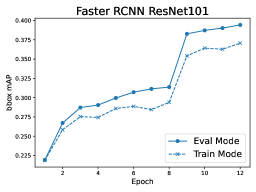
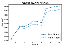
Figure 4: Training curve of Faster RCNN with ResNet101 and HRNet backbone. Models trained in Train Mode shows noticeable performance deterioration compared to Eval Mode.

Appendix D Original data of object classification

The below settings are taken from the default values in the TLlib library: ResNet50 is the backbone network and all parameters are optimized by Stochastic Gradient Descent with 0.9 momentum and 0.0005 weight decay. Each training process consisted of 20 epochs, with 500 iterations per epoch. We set the initial learning rates to 0.001 and 0.01 for the feature extractor and linear projection head respectively, and scheduled the learning rates of all layers to decay by 0.1 at epochs 8 and 12. The input images were all resized and cropped to 448 $\times$ 448, and the batch size was fixed at 48. Since the backbone network takes the major computation, the memory and time in three different dataset are very similar.

Dataset	Mode	Trial 1 Accuracy	Trial 2 Accuracy	Trial 3 Accuracy	Average Accuracy	Std
CUB-200-Birds	Train	83.20	83.10	82.90	83.07	0.15
	Tune	83.20	83.20	83.20	83.20	0.00
Aircrafts	Train	85.40	85.20	85.60	85.40	0.20
	Tune	86.00	85.60	86.10	85.90	0.26
Stanford Cars	Train	89.90	89.90	89.80	89.87	0.06
	Tune	90.20	90.00	90.20	90.13	0.12

Table 7: Original data of object classification experiments for calculating mean and standard deviation.

Appendix E Efficiency Comparison Between Tune and Deploy

Table 8: Efficiency comparison between Eval, Tune and Deploy. Time is measured by second/iteration and the memory is the peak memory footprint (GB) during forward and backward. We can observe that $\text{Deploy}\approx\text{Tune}>\text{Eval}$ in terms of efficiency.

Batch Size	Input Size	Eval Mode		Tune Mode		DeployMode
		Time	Memory	Time	Memory	Time	Memory
32	224	0.0945	2.8237	0.0849	1.5973	0.0830	1.5619
32	256	0.1110	3.5965	0.1032	1.9732	0.1011	1.9416
32	288	0.1488	4.5130	0.1382	2.4325	0.1356	2.3728
32	320	0.1761	5.5216	0.1630	2.9207	0.1609	2.8363
32	352	0.2153	6.6120	0.1991	3.4546	0.1969	3.3682
32	384	0.2503	7.9005	0.2304	4.0995	0.2281	4.0219
32	416	0.2983	9.2317	0.2738	4.7429	0.2721	4.6640
32	448	0.3567	10.6448	0.3104	5.4306	0.3077	5.3421
16	224	0.0505	1.5671	0.0467	0.9727	0.0448	0.9397
32	224	0.0948	2.8237	0.0849	1.5973	0.0831	1.5631
64	224	0.1837	5.4125	0.1613	2.8617	0.1590	2.7808
128	224	0.3577	10.6001	0.3081	5.4088	0.3060	5.3284
256	224	0.7035	21.0107	0.6001	10.5011	0.5966	10.4234

Appendix F Comparing with Inplace-ABN

Table 9: Comparision between proposed Tune Mode and the Inplace-ABN (Bulo et al., 2018). We can observe that Inplace-ABN saves memory at the cost of speed and accuracy, while Tune mode saves memory at no cost of computation time or accuracy.

Dataset	Method	Accuracy	Memory (GB)	Time (second/iteration)
CUB-200	Baseline	$\text{83.07}_{\pm 0.15}$	19.967	0.571
	Inplace-ABN	$\text{74.80}_{\pm 0.21}$ (8.27$\downarrow$)	16.739 (16.17%$\downarrow$)	0.623 (9.10%$\uparrow$)
	Tune Mode (ours)	$\textbf{83.20}_{\pm 0.00}$ (0.13$\uparrow$)	12.323 (38.28%$\downarrow$)	0.501 (12.26%$\downarrow$)
Aircraft	Baseline	$\text{85.40}_{\pm 0.20}$	19.965	0.564
	Inplace-ABN	$\text{78.23}_{\pm 0.45}$ (7.17$\downarrow$)	16.737 (16.17%$\downarrow$)	0.620 (8.58%$\uparrow$)
	Tune Mode (ours)	$\textbf{85.90}_{\pm 0.26}$ (0.50$\uparrow$)	12.323 (38.28%$\downarrow$)	0.505 (10.51%$\downarrow$)
Stanford Car	Baseline	$\text{89.87}_{\pm 0.06}$	19.967	0.571
	Inplace-ABN	$\text{86.30}_{\pm 0.28}$ (3.57$\downarrow$)	16.739 (16.17%$\downarrow$)	0.614 (7.53%$\uparrow$)
	Tune Mode (ours)	$\textbf{90.13}_{\pm 0.12}$ (0.26$\uparrow$)	12.321 (38.28%$\downarrow$)	0.491 (14.00%$\downarrow$)

Appendix G Small Randomness in Object Detection

The high computational cost limited us to repeating the experiment only once for validating small randomness in object detection. We conducted three trials of the Faster RCNN ResNet50 standard configuration and obtained an average best mAP of 0.3748, 0.3735, and 0.3739, with a standard deviation of 0.000543. These results demonstrate that object detection tasks have very little randomness.

Appendix H Estimation of Total Computation Used in This Paper

Each trial of classification experiments in Section 4.1 requires about $2$ hours of V100 GPU training. The numbers reported in this paper requires 18 trials, which cost about $36$ GPU hours.

Each trial of detection experiments in Section 4.2 requires about $12$ hours of 8 V100 GPU training, which is $96$ GPU hours. The numbers reported in this paper requires 25 trials, which cost about $2400$ GPU hours.

Each trial of pre-training experiments in Section I requires about $24$ hours of 8 V100 GPU training, which is $192$ GPU hours. The numbers reported in this paper requires about $\frac{5}{3}$ full trials, which cost about $320$ GPU hours.

Some experiments for the purpose of analyses also cost computation. Figure 2 requires two trials of object detection and 6 trials of object classification, with about $204$ GPU hours. Figure 4 requires four trials of object detection, with about $384$ GPU hours.

Summing the above numbers up, and considering all the fractional computation for the rest analyses experiments, this paper costs about $3400$ GPU hours.

Considering the cost of prototyping and previous experiments that do not get into the paper, the total cost of this project is about $5000$ GPU hours.

Note that these numbers are rough estimation of the cost, and do not include the additional cost for storing data/system maintenance etc.

Appendix I Beyond Transfer Learning

Tune mode is designed for transfer learning because it requires tracked statistics to normalize features. Here we show that Tune mode can also be used in late stages of pre-training. We use the prevalent ImageNet pre-training as baseline, which has three stages with decaying learning rate. We tried to turn on Tune mode at the third stage, the accuracy slightly dropped. Nevertheless, due to our implementation with torch.fx, we can dynamically switch the mode during training. Therefore, we also tried to alternate between Train mode and Tune mode at the third stage, which retained the accuracy with less computation time.

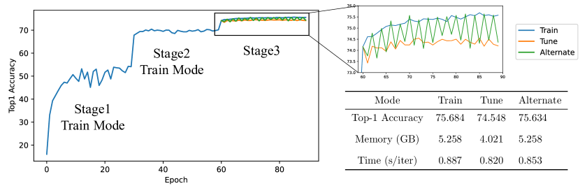
Figure 5: ImageNet Pre-training Results

Appendix J Broader Impact and Limitations

This paper’s broader impact lies in its potential to significantly improve the efficiency of transfer learning in ConvBN blocks, a cornerstone of many computer vision tasks and other domains. By introducing the novel Tune Mode, we offer a solution that bridges the gap between the computational efficiency of Deploy Mode and the training stability of Eval Mode. This development could benefit a wide range of applications, including real-time object detection, image classification, and other tasks that rely heavily on transfer learning.

Moreover, the reduction in GPU memory footprint and training time could democratize access to advanced machine learning techniques, as it lowers the computational resources required. This could enable smaller research groups, startups, and institutions in developing countries to participate in cutting-edge AI research and development.

However, it’s also important to consider potential negative impacts. The increased efficiency could potentially be used in applications with harmful intent, such as deepfake generation or surveillance technologies. Additionally, while our method reduces the computational resources required, it may still be inaccessible to those without any access to GPUs or similar hardware.

The proposed Tune Mode is designed for transfer learning, and we have a preliminary experiment for pre-training. How to enable efficient pre-training with ConvBN blocks would be an important topic in the future. In addition, it is not clear if we can develop similar methods for normalizations other than BatchNorm. Currently, it seems this technique is only applicable to ConvBN blocks with BatchNorm.

References

- Ba et al. [2016] Jimmy Lei Ba, Jamie Ryan Kiros, and Geoffrey E. Hinton. Layer Normalization. 2016.
- Bishop [2006] Christopher M. Bishop. Pattern recognition and machine learning. 2006.
- Bommasani et al. [2022] Rishi Bommasani, Drew A. Hudson, Ehsan Adeli, Russ Altman, Simran Arora, Sydney von Arx, Michael S. Bernstein, Jeannette Bohg, Antoine Bosselut, Emma Brunskill, Erik Brynjolfsson, Shyamal Buch, Dallas Card, Rodrigo Castellon, Niladri Chatterji, Annie Chen, Kathleen Creel, Jared Quincy Davis, Dora Demszky, Chris Donahue, Moussa Doumbouya, Esin Durmus, Stefano Ermon, John Etchemendy, Kawin Ethayarajh, Li Fei-Fei, Chelsea Finn, Trevor Gale, Lauren Gillespie, Karan Goel, Noah Goodman, Shelby Grossman, Neel Guha, Tatsunori Hashimoto, Peter Henderson, John Hewitt, Daniel E. Ho, Jenny Hong, Kyle Hsu, Jing Huang, Thomas Icard, Saahil Jain, Dan Jurafsky, Pratyusha Kalluri, Siddharth Karamcheti, Geoff Keeling, Fereshte Khani, Omar Khattab, Pang Wei Koh, Mark Krass, Ranjay Krishna, Rohith Kuditipudi, Ananya Kumar, Faisal Ladhak, Mina Lee, Tony Lee, Jure Leskovec, Isabelle Levent, Xiang Lisa Li, Xuechen Li, Tengyu Ma, Ali Malik, Christopher D. Manning, Suvir Mirchandani, Eric Mitchell, Zanele Munyikwa, Suraj Nair, Avanika Narayan, Deepak Narayanan, Ben Newman, Allen Nie, Juan Carlos Niebles, Hamed Nilforoshan, Julian Nyarko, Giray Ogut, Laurel Orr, Isabel Papadimitriou, Joon Sung Park, Chris Piech, Eva Portelance, Christopher Potts, Aditi Raghunathan, Rob Reich, Hongyu Ren, Frieda Rong, Yusuf Roohani, Camilo Ruiz, Jack Ryan, Christopher Ré, Dorsa Sadigh, Shiori Sagawa, Keshav Santhanam, Andy Shih, Krishnan Srinivasan, Alex Tamkin, Rohan Taori, Armin W. Thomas, Florian Tramèr, Rose E. Wang, William Wang, Bohan Wu, Jiajun Wu, Yuhuai Wu, Sang Michael Xie, Michihiro Yasunaga, Jiaxuan You, Matei Zaharia, Michael Zhang, Tianyi Zhang, Xikun Zhang, Yuhui Zhang, Lucia Zheng, Kaitlyn Zhou, and Percy Liang. On the Opportunities and Risks of Foundation Models, 2022.
- Bouvrie [2006] Jake Bouvrie. Notes on convolutional neural networks. 2006.
- Boyd and Vandenberghe [2004] Stephen Boyd and Lieven Vandenberghe. Convex optimization. 2004.
- Bulo et al. [2018] Samuel Rota Bulo, Lorenzo Porzi, and Peter Kontschieder. In-place activated batchnorm for memory-optimized training of dnns. In CVPR, 2018.
- Chen et al. [2019] Kai Chen, Jiaqi Wang, Jiangmiao Pang, Yuhang Cao, Yu Xiong, Xiaoxiao Li, Shuyang Sun, Wansen Feng, Ziwei Liu, and Jiarui Xu. MMDetection: Open mmlab detection toolbox and benchmark. arXiv preprint arXiv:1906.07155, 2019.
- Deng et al. [2009] Jia Deng, Wei Dong, Richard Socher, Li-Jia Li, Kai Li, and Li Fei-Fei. Imagenet: A large-scale hierarchical image database. In CVPR, 2009.
- Donahue et al. [2014] Jeff Donahue, Yangqing Jia, Oriol Vinyals, Judy Hoffman, Ning Zhang, Eric Tzeng, and Trevor Darrell. Decaf: A deep convolutional activation feature for generic visual recognition. In ICML, 2014.
- Gupta et al. [2019] Tanmay Gupta, Alexander Schwing, and Derek Hoiem. No-frills human-object interaction detection: Factorization, layout encodings, and training techniques. In CVPR, 2019.
- Harris et al. [2020] Charles R. Harris, K. Jarrod Millman, Stéfan J. Van Der Walt, Ralf Gommers, Pauli Virtanen, David Cournapeau, Eric Wieser, Julian Taylor, Sebastian Berg, and Nathaniel J. Smith. Array programming with NumPy. Nature, 2020.
- He et al. [2016] Kaiming He, Xiangyu Zhang, Shaoqing Ren, and Jian Sun. Deep residual learning for image recognition. In CVPR, 2016.
- Huang et al. [2023] Lei Huang, Jie Qin, Yi Zhou, Fan Zhu, Li Liu, and Ling Shao. Normalization techniques in training dnns: Methodology, analysis and application. TPAMI, 2023.
- Ioffe [2017] Sergey Ioffe. Batch renormalization: Towards reducing minibatch dependence in batch-normalized models. In Advances in neural information processing systems, 2017.
- Ioffe and Szegedy [2015] Sergey Ioffe and Christian Szegedy. Batch Normalization: Accelerating Deep Network Training by Reducing Internal Covariate Shift. In ICML, 2015.
- Jiang et al. [2022] Junguang Jiang, Yang Shu, Jianmin Wang, and Mingsheng Long. Transferability in deep learning: A survey. arXiv preprint arXiv:2201.05867, 2022.
- Krause et al. [2013] Jonathan Krause, Michael Stark, Jia Deng, and Li Fei-Fei. 3d object representations for fine-grained categorization. In Proceedings of the IEEE international conference on computer vision workshops, pages 554–561, 2013.
- Kuznetsova et al. [2018] Alina Kuznetsova, Hassan Rom, Neil Alldrin, Jasper Uijlings, Ivan Krasin, Jordi Pont-Tuset, Shahab Kamali, Stefan Popov, Matteo Malloci, and Tom Duerig. The open images dataset v4: Unified image classification, object detection, and visual relationship detection at scale. arXiv preprint arXiv:1811.00982, 2018.
- LeCun et al. [1998] Yann LeCun, Léon Bottou, Yoshua Bengio, and Patrick Haffner. Gradient-based learning applied to document recognition. Proc. IEEE, 1998.
- Lin et al. [2014] Tsung-Yi Lin, Michael Maire, Serge Belongie, James Hays, Pietro Perona, Deva Ramanan, Piotr Dollár, and C. Lawrence Zitnick. Microsoft coco: Common objects in context. In ECCV, 2014.
- Maas et al. [2013] Andrew L. Maas, Awni Y. Hannun, and Andrew Y. Ng. Rectifier nonlinearities improve neural network acoustic models. In ICML, 2013.
- Mahajan et al. [2018] Dhruv Mahajan, Ross Girshick, Vignesh Ramanathan, Kaiming He, Manohar Paluri, Yixuan Li, Ashwin Bharambe, and Laurens van der Maaten. Exploring the limits of weakly supervised pretraining. In ECCV, 2018.
- Maji et al. [2013] Subhransu Maji, Esa Rahtu, Juho Kannala, Matthew Blaschko, and Andrea Vedaldi. Fine-grained visual classification of aircraft. arXiv preprint arXiv:1306.5151, 2013.
- Markuš [2018] Nenad Markuš. Fusing batch normalization and convolution in runtime. https://nenadmarkus.com/p/fusing-batchnorm-and-conv/, 2018.
- Micikevicius et al. [2018] Paulius Micikevicius, Sharan Narang, Jonah Alben, Gregory Diamos, Erich Elsen, David Garcia, Boris Ginsburg, Michael Houston, Oleksii Kuchaiev, Ganesh Venkatesh, and Hao Wu. Mixed Precision Training. In ICLR, 2018.
- Nair and Hinton [2010] Vinod Nair and Geoffrey E. Hinton. Rectified linear units improve restricted boltzmann machines. In ICML, 2010.
- Paszke et al. [2019] Adam Paszke, Sam Gross, Francisco Massa, Adam Lerer, James Bradbury, Gregory Chanan, Trevor Killeen, Zeming Lin, Natalia Gimelshein, Luca Antiga, Alban Desmaison, Andreas Kopf, Edward Yang, Zachary DeVito, Martin Raison, Alykhan Tejani, Sasank Chilamkurthy, Benoit Steiner, Lu Fang, Junjie Bai, and Soumith Chintala. PyTorch: An Imperative Style, High-Performance Deep Learning Library. In NeurIPS, 2019.
- Rabiner and Gold [1975] Lawrence R. Rabiner and Bernard Gold. Theory and application of digital signal processing. Englewood Cliffs: Prentice-Hall, 1975.
- Radosavovic et al. [2020] Ilija Radosavovic, Raj Prateek Kosaraju, Ross Girshick, Kaiming He, and Piotr Dollár. Designing network design spaces. In CVPR, 2020.
- Reed et al. [2022] James Reed, Zachary DeVito, Horace He, Ansley Ussery, and Jason Ansel. torch. fx: Practical Program Capture and Transformation for Deep Learning in Python. In MLSys, 2022.
- Ren et al. [2015] Shaoqing Ren, Kaiming He, Ross Girshick, and Jian Sun. Faster R-CNN: Towards Real-Time Object Detection with Region Proposal Networks. In NeurIPS, 2015.
- Ulyanov et al. [2016] Dmitry Ulyanov, Andrea Vedaldi, and Victor Lempitsky. Instance normalization: The missing ingredient for fast stylization. arXiv preprint arXiv:1607.08022, 2016.
- Vanholder [2016] Han Vanholder. Efficient inference with tensorrt. In GPU Technology Conference, 2016.
- Wah et al. [2011] Catherine Wah, Steve Branson, Peter Welinder, Pietro Perona, and Serge Belongie. The caltech-ucsd birds-200-2011 dataset. 2011.
- Wang et al. [2021] Dequan Wang, Evan Shelhamer, Shaoteng Liu, Bruno Olshausen, and Trevor Darrell. Tent: Fully Test-Time Adaptation by Entropy Minimization. In ICLR, 2021.
- Wang et al. [2020] Jingdong Wang, Ke Sun, Tianheng Cheng, Borui Jiang, Chaorui Deng, Yang Zhao, Dong Liu, Yadong Mu, Mingkui Tan, and Xinggang Wang. Deep high-resolution representation learning for visual recognition. TPAMI, 2020.
- Wang et al. [2022] Qin Wang, Olga Fink, Luc Van Gool, and Dengxin Dai. Continual Test-Time Domain Adaptation. In CVPR, 2022.
- Wang et al. [2019] Ximei Wang, Ying Jin, Mingsheng Long, Jianmin Wang, and Michael I. Jordan. Transferable Normalization: Towards Improving Transferability of Deep Neural Networks. In NeurIPS, 2019.
- Wu and He [2018] Yuxin Wu and Kaiming He. Group Normalization. In ECCV, 2018.
- Xie et al. [2017] Saining Xie, Ross Girshick, Piotr Dollár, Zhuowen Tu, and Kaiming He. Aggregated residual transformations for deep neural networks. In CVPR, 2017.
- Zhou et al. [2018] B. Zhou, A. Lapedriza, A. Khosla, A. Oliva, and A. Torralba. Places: A 10 Million Image Database for Scene Recognition. TPAMI, 2018.