Nonconvex Robust High-Order Tensor Completion Using Randomized Low-Rank Approximation

Abstract

Within the tensor singular value decomposition (T-SVD) framework, existing robust low-rank tensor completion approaches have made great achievements in various areas of science and engineering. Nevertheless, these methods involve the T-SVD based low-rank approximation, which suffers from high computational costs when dealing with large-scale tensor data. Moreover, most of them are only applicable to third-order tensors. Against these issues, in this article, two efficient low-rank tensor approximation approaches fusing randomized techniques are first devised under the order-$d$ ($d\geq 3$) T-SVD framework. On this basis, we then further investigate the robust high-order tensor completion (RHTC) problem, in which a double nonconvex model along with its corresponding fast optimization algorithms with convergence guarantees are developed. To the best of our knowledge, this is the first study to incorporate the randomized low-rank approximation into the RHTC problem. Empirical studies on large-scale synthetic and real tensor data illustrate that the proposed method outperforms other state-of-the-art approaches in terms of both computational efficiency and estimated precision.

I Introduction

Multidimensional data including medical images, remote sensing images, light field images, color videos, and beyond, are becoming increasingly prevailing in various domains such as neuroscience [1], chemometrics [2], data mining [3], machine learning [4], image processing [5, 6, 7], and computer vision [8, 9, 10]. Compared to vectors and matrices, tensors possess a more powerful capability to characterize the inherent structural information underlying these data from a higher-order perspective. Nevertheless, due to various factors such as occlusions, abnormalities, software glitches, or sensor failures, the tensorial data faced in practical applications can often suffer from elements loss and noise/outliers corruption. Hence, robust low-rank tensor completion (RLRTC) has been widely concerned by a large number of scholars [11, 12, 13, 14, 15, 16, 17, 18, 19, 20, 21, 22, 23, 24, 25, 26, 27, 28, 29, 30].

RLRTC belongs to a canonical inverse problem, which aims to reconstruct the underlying low-rank tensor from partial observations of target tensor corrupted by noise/outliers. Mathematically, the RLRTC model can be formulated as follows:

$$\min_{{\boldsymbol{\mathcal{L}}},{\boldsymbol{\mathcal{E}}}}\;\;\Psi({\boldsymbol{\mathcal{L}}})+\lambda\Upsilon({\boldsymbol{\mathcal{E}}}),\;\;\text{s.t.}\;\;\boldsymbol{\bm{P}}_{{{\Omega}}}({\boldsymbol{\mathcal{L}}}+{\boldsymbol{\mathcal{E}}})=\boldsymbol{\bm{P}}_{{{\Omega}}}({\boldsymbol{\mathcal{M}}}),$$ (1)

where $\Psi({\boldsymbol{\mathcal{L}}})$ represents the regularizer measuring tensor low-rankness (also called the certain relaxation of tensor rank), $\Upsilon({\boldsymbol{\mathcal{E}}})$ denotes the noise/outliers regularization, $\lambda>0$ is a trade-off parameter that balances these two terms, ${\boldsymbol{\mathcal{M}}}$ is the observed tensor, and $\boldsymbol{\bm{P}}_{{{\Omega}}}(\cdot)$ is the projection operator onto the observed index set ${{{\Omega}}}$ such that

$$\big{(}\boldsymbol{\bm{P}}_{{{\Omega}}}(\boldsymbol{\mathcal{M}})\big{)}_{i_{1},\cdots,i_{d}}=\begin{cases}{\boldsymbol{\mathcal{M}}}_{i_{1},\cdots,i_{d}},\;\text{if}\;(i_{1},\cdots,i_{d})\in\Omega,\\ 0,\;\;\;\;\;\;\;\;\;\;\;\;\;\text{otherwise}.\end{cases}$$

If the index set ${{{\Omega}}}$ is the whole set, i.e., no elements are missing, then the model (1) reduces to the Tensor Robust Principal Component Analysis (TRPCA) problem [31, 32, 33, 34, 35, 36, 37, 38, 39]. If there is no corruption, i.e., ${\boldsymbol{\mathcal{E}}}=0$, then the model (1) is equivalent to the Low-Rank Tensor Completion (LRTC) problem [40, 41, 42, 43, 44, 45, 46, 47, 48, 49]. Therefore, RLRTC can be viewed as a generalized form of both LRTC and TRPCA.

Nevertheless, there exist different definitions of tensor rank and its corresponding relaxation within different tensor decomposition frameworks, which makes the optimization problem (1) extremely complicated. The commonly-used frameworks contain CANDECOMP/PARAFAC (CP) [50], Tucker [51], tensor train (TT) [52], tensor ring (TR) [53], and tensor singular value decomposition (T-SVD) [54, 55]. Among them, T-SVD presents the first closed multiplication operation called tensor-tensor product (t-product), and derives a novel tensor tubal rank [56] that well characterizes the intrinsic low-rank structure of a tensor. In particular, the recent work [57] revolutionarily proved the best representation and compression theories of T-SVD, making it more notable in capturing the “spatial-shifting” correlation and the global structure information underlying tensors. With these advantages, the robust low-tubal-rank tensor completion [20, 21, 22, 23, 24, 25, 26, 27, 28, 29, 30] modeled by (1) and its variants [31, 32, 33, 34, 35, 36, 37, 38, 39, 40, 41, 42, 43, 44] have recently caught many scholars’ attention. However, we observe that these approaches are only relevant to third-order tensors. To fix this problem, Qin et al. established an order-$d$ ($d\geq 3$) T-SVD algebraic framework [58] based on a family of invertible linear transforms, and then preliminary investigated the model, algorithm, and theory for the robust high-order tensor completion (RHTC) [58, 59, 60, 61]. The RHTC methods generated by other tensor factorization frameworks can be found in [11, 12, 13, 14, 15, 16, 17, 18, 19].

Although the above deterministic RLRTC investigations have already made some achievements in real-world applications, they encounter enormous challenges in dealing with those tensorial data characterized by large volumes, high dimensions, complex structures, etc. This is mainly attributed to the fact that they require to perform multiple low-rank approximations based on a specific tensor factorization. Calculating such an approximation generally involves the singular value decomposition (SVD) or T-SVD, which is very time-consuming and inefficient when the data size scales up. Motivated by the reason that randomized algorithms can accelerate the computational speed of their conventional counterparts at the expense of slight accuracy loss [62, 63, 64, 65, 66], effective low-rank tensor approximation approaches using randomized sketching techniques (e.g., [67, 68, 69, 70, 71, 72, 73, 74, 75]) have attracted more and more attention in recent years. Among these methods, we obviously find that the ones based on T-SVD framework are only appropriate for third-order tensors. In addition, RHTC researches in combination with randomized low-rank approximation are relatively lacking. With the rapid development of information technologies, such as Internet of Things, and big data, large-scale high-order tensors encountered in real scenarios are growing explosively, like order-four color videos and multi-temporal remote sensing images, order-five light filed images, order-six bidirectional texture function images. Therefore, in this work, we consider developing fast and efficient randomness-based large-scale high-order tensor representation and recovery methods under the T-SVD framework.

I-A Our Contributions

Main contributions of this work are summarized as follows:

1) Firstly, within the order-$d$ T-SVD algebraic framework [58], two efficient randomized algorithms for low-rank approximation of high-order tensor are devised considering their adaptability to large-scale tensor data. The developed approximation methods obtain a significant advantage in computational speed against the optimal $k$-term approximation [58] (also called truncated T-SVD) with a slight loss of precision.

2) Secondly, an effective and scalable model for RHTC is proposed in virtue of nonconvex low-rank and noise/outliers regularizers. Based on the proposed randomized low-rank approximation schemes, we then design two alternating direction method of multipliers (ADMM) framework based fast algorithms with convergence guarantees to solve the formulated model, through which any low T-SVD rank high-order tensors with simultaneous elements loss and noise/outliers corruption can be reconstructed efficiently and accurately.

3) Thirdly, our proposed RHTC algorithm can be applied to a series of large-scale reconstruction tasks, such as the restoration of fourth-order color videos and multi-temporal remote sensing images, and fifth-order light-field images. Experimental results demonstrate that the proposed method achieves competitive performance in estimation accuracy and CPU running time than other state-of-the-art ones. Strikingly, in the case of sacrificing a little precision, our versions combined with randomization ideas decrease the CPU time by about $50\%$$\sim$$70\%$ compared with the deterministic version.

I-B Organization

The remainder of the paper is organized as follows. Section II gives a brief summary of related work. The main notations and preliminaries are introduced in Section III, and then we develop two efficient randomized algorithms for low-rank approximation of high-order tensor in Section IV. Section V proposes effective nonconvex model and optimization algorithm for RHTC. In Section VI, extensive experiments are conducted to evaluate the effectiveness of the proposed method. Finally, we conclude our work in Section VII.

What is noteworthy is that this article can be regarded as an expanded version of our previous conference paper [60]. Built off the conference version, this paper makes the following changes: 1) the high-order tensor approximation algorithm that fuses the randomized blocked strategy is added; 2) the original low-rank and noise/outliers regularizers are further enhanced with more flexible regularizers; 3) two accelerated algorithms for solving the newly formulated non-convex model are designed via the proposed low-rank approximation strategies; 4) a large number of experiments concerning with high-order tensor approximation and restoration are added.

TABLE I: The main notions and preliminaries for order-$d$ tensor.

Notations	Descriptions	Notations	Descriptions
${{\bm{A}}}\in\mathbb{R}^{n_{1}\times n_{2}}$	matrix	$\bm{I}_{n}\in\mathbb{R}^{n\times n}$	$n\times n$ identity matrix
$\operatorname{trace}(\bm{A})$	matrix trace	${{\bm{A}}}^{\mit{H}}({{\bm{A}}}^{\mit{T}})$	conjugate transpose (transpose)
$\langle{{\bm{A}}},{{\bm{B}}}\rangle=\operatorname{trace}({{\bm{A}}}^{\mit{H}}\cdot{{\bm{B}}})$	matrix inner product	${\|{{\bm{A}}}\|}_{\bm{w},{\mathrm{S}}_{p}}={\big{(}\sum_{i}{\bm{w}}_{i}\;\big{|}\sigma_{i}({{\bm{A}}})\big{|}^{p}\big{)}}^{\frac{1}{p}}$	matrix weighted Schatten-$p$ norm
${\boldsymbol{\mathcal{A}}}\in\mathbb{R}^{n_{1}\times\cdots\times n_{d}}$	order-$d$ tensor	${\boldsymbol{\mathcal{A}}}_{i_{1}\cdots i_{d}}$ or ${\boldsymbol{\mathcal{A}}}{(i_{1},\cdots,i_{d})}$	$(i_{1},\cdots,i_{d})$-th entry
${{\bm{A}}_{(k)}}\in\mathbb{R}^{n_{k}\times\prod_{j\neq k}{n_{j}}}$	mode-$k$ unfolding of $\boldsymbol{\mathcal{A}}$	${\|{\boldsymbol{\mathcal{A}}}\|}_{\infty}=\max_{i_{1}\cdots i_{d}}|{\boldsymbol{\mathcal{A}}_{i_{1}\cdots i_{d}}}|$	tensor infinity norm
${\|{\boldsymbol{\mathcal{A}}}\|}_{{\boldsymbol{\mathcal{W}}},\ell_{q}}=({\sum}{\boldsymbol{\mathcal{W}}_{i_{1}\cdots i_{d}}}|{\boldsymbol{\mathcal{A}}_{i_{1}\cdots i_{d}}}|^{q})^{\frac{1}{q}}$	tensor weighted $\ell_{q}$-norm	${\|{\boldsymbol{\mathcal{A}}}\|}_{\mathnormal{F}}={(\sum_{i_{1}\cdots i_{d}}|{\boldsymbol{\mathcal{A}}_{i_{1}\cdots i_{d}}}|^{2})^{\frac{1}{2}}}$	tensor Frobenius norm
$\boldsymbol{\mathcal{C}}={\boldsymbol{\mathcal{A}}}{*}_{\mathfrak{L}}{\boldsymbol{\mathcal{B}}}$	order-$d$ t-product under linear transform $\mathfrak{L}$	${{\boldsymbol{\mathcal{A}}}}^{\mit{H}}({{\boldsymbol{\mathcal{A}}}}^{\mit{T}})$	transpose (conjugate transpose)
$\langle{\boldsymbol{\mathcal{A}}},{\boldsymbol{\mathcal{B}}}\rangle$	the inner product between order-$d$ tensors ${\boldsymbol{\mathcal{A}}}$ and ${\boldsymbol{\mathcal{B}}}$, i.e., $\langle{\boldsymbol{\mathcal{A}}},{\boldsymbol{\mathcal{B}}}\rangle={\sum}_{j=1}^{n_{3}n_{4}\cdots n_{d}}\langle{\bm{\mathcal{A}}}^{<j>},{\bm{\mathcal{B}}}^{<j>}\rangle$.
${\boldsymbol{\mathcal{A}}}^{<j>}\in\mathbb{R}^{n_{1}\times n_{2}}$	the matrix frontal slice of ${\boldsymbol{\mathcal{A}}}$, ${\boldsymbol{\mathcal{A}}}^{<j>}={\boldsymbol{\mathcal{A}}}{(:,:,i_{3},\cdots,i_{d})},\;j={\sum_{a=4}^{d}}{(i_{a}-1){\Pi}_{b=3}^{a-1}n_{b}}+i_{3}$ .
$\boldsymbol{\mathcal{A}}\;{\times}_{n}\;\bm{M}$	the mode-$n$ product of tensor $\boldsymbol{\mathcal{A}}$ with matrix ${\bm{M}},\;\boldsymbol{\mathcal{B}}=\boldsymbol{\mathcal{A}}{\times}_{n}{\bm{M}}$ $\Longleftrightarrow$ ${\bm{B}}_{(n)}={\bm{M}}\cdot{\bm{A}}_{(n)}$.
${\operatorname{bdiag}}({{\boldsymbol{\mathcal{A}}}})\in\mathbb{R}^{n_{1}n_{3}\cdots n_{d}\times n_{2}n_{3}\cdots n_{d}}$	${\operatorname{bdiag}}({{\boldsymbol{\mathcal{A}}}})$ is a block diagonal matrix whose $i$-th block equals to ${\boldsymbol{\mathcal{A}}}^{<i>}$, $\forall i\in\{1,2,\cdots,n_{3}\cdots n_{d}\}$.
f-diagonal/f-upper triangular tensor ${\boldsymbol{\mathcal{A}}}$	frontal slice ${\boldsymbol{\mathcal{A}}}^{<j>}$ of ${\boldsymbol{\mathcal{A}}}$ is a diagonal matrix (an upper triangular matrix), $\forall j\in\{1,2,\cdots,n_{3}\cdots n_{d}\}$.
identity tensor ${\boldsymbol{\mathcal{I}}}\in\mathbb{R}^{n\times n\times n_{3}\times\cdots\times n_{d}}$	identity tensor ${\boldsymbol{\mathcal{I}}}$ is defined to be a tensor such that ${{\mathfrak{L}}({\boldsymbol{\mathcal{I}}})}^{<j>}=\bm{I}_{n},\forall j\in\{1,2,\cdots,n_{3}\cdots n_{d}\}$.
Gaussian random tensor ${\boldsymbol{\mathcal{G}}}$	the entries of ${{\mathfrak{L}}({\boldsymbol{\mathcal{G}}})}^{<j>}$ follow the standard normal distribution, $\forall j\in\{1,2,\cdots,n_{3}\cdots n_{d}\}$.
orthogonal tensor ${\boldsymbol{\mathcal{Q}}}$	orthogonal tensor satisfies: ${\boldsymbol{\mathcal{Q}}}^{\mit{T}}{*}_{\mathfrak{L}}{\boldsymbol{\mathcal{Q}}}={\boldsymbol{\mathcal{Q}}}{*}_{\mathfrak{L}}{\boldsymbol{\mathcal{Q}}}^{\mit{T}}={\boldsymbol{\mathcal{I}}}$, while partially orthogonal tensor satisfies: ${\boldsymbol{\mathcal{Q}}}^{\mit{T}}{*}_{\mathfrak{L}}{\boldsymbol{\mathcal{Q}}}={\boldsymbol{\mathcal{I}}}$.
$\textrm{H-TSVD}({\boldsymbol{\mathcal{A}}},\mathfrak{L})$	order-$d$ T-SVD factorization, i.e., ${\boldsymbol{\mathcal{A}}}={\boldsymbol{\mathcal{U}}}{*}_{\mathfrak{L}}{\boldsymbol{\mathcal{S}}}{*}_{\mathfrak{L}}{\boldsymbol{\mathcal{V}}}^{\mit{T}}$, where ${\boldsymbol{\mathcal{U}}}$ and ${\boldsymbol{\mathcal{V}}}$ are orthogonal, ${\boldsymbol{\mathcal{S}}}$ is f-diagonal.
$\textrm{H-TQR}({\boldsymbol{\mathcal{A}}},\mathfrak{L})$	order-$d$ tensor QR-type factorization, i.e., ${\boldsymbol{\mathcal{A}}}={\boldsymbol{\mathcal{Q}}}{*}_{\mathfrak{L}}{\boldsymbol{\mathcal{R}}}$, where ${\boldsymbol{\mathcal{Q}}}$ is orthogonal while ${\boldsymbol{\mathcal{R}}}$ is f-upper triangular.
${\operatorname{rank}}_{tsvd}({{\boldsymbol{\mathcal{A}}}})$	${\operatorname{rank}}_{tsvd}({\boldsymbol{\mathcal{A}}})=\sum_{i}{\mathbbm{1}\big{[}{\boldsymbol{\mathcal{S}}}(i,i,:,\cdots,:)\neq\boldsymbol{0}\big{]}}$, where ${\boldsymbol{\mathcal{S}}}$ originates from the middle component of ${\boldsymbol{\mathcal{A}}}={\boldsymbol{\mathcal{U}}}{{*}_{\mathfrak{L}}}{\boldsymbol{\mathcal{S}}}{*}_{\mathfrak{L}}{\boldsymbol{\mathcal{V}}}^{\mit{T}}$.

II Related Work

Based on different factorization schemes, the representative RLRTC methods can be broadly summarized as follows.

II-1 RLRTC Based on T-SVD Factorization

Lu et al. [31] rigorously deduced a novel tensor nuclear norm (TNN) corresponding to T-SVD that is proved to be the convex envelope of the tensor average rank. Sequentially, Jiang et al. [20] conducted a rigourous study for the RLRTC problem, which is modeled by the TNN and $\ell_{1}$-norm penalty terms. Besides, Wang et al. also adopted this novel TNN or slice-weighted TNN plus a sparsity measure inducing $\ell_{1}$-norm to develop the RLRTC methods [21, 22]. Theoretically, the deterministic and non-asymptotic upper bounds on the estimation error are established from a statistical standpoint. However, the previous methods may suffer from disadvantage due to the limitation of Fourier transform [29]. Aiming at this issue, by utilizing the generalized transformed TNN (TTNN) and $\ell_{1}$-norm regularizers, Song et al. [24] proposed an unitary transform method for RLRTC and also analyzed its recovery guarantee. Continuing along this vein, a patched-tubes unitary transform approach for RLRTC was proposed by Ng et al. [25]. Nevertheless, the TTNN is a loose approximation of the tensor tubal rank, which usually leads to the over-penalization of the optimization problem and hence causes some unavoidable biases in real applications. In addition, as indicated by [76], the $\ell_{1}$-norm might not be statistically optimal in more challenging scenarios. Recently, to break the shortcomings existing in the TNN and $\ell_{1}$-norm regularization terms, some researchers [27, 28, 29, 30] designed new nonconvex low-rank and noise/outliers regularization terms to study the RLRTC problem from the model, algorithm, and theory. But these methods are only limited to the case of third-order tensors and face the high computational expense of T-SVD.

II-2 RLRTC Based on Other Factorization Schemes

Liu et al. [45] primitively developed a new Tucker nuclear norm, i.e., Sum-of-Nuclear-Norms of unfolding matrices of a tensor (SNN), as convex relaxation of the tensor tucker rank. Then, the RLRTC approach within the Tucker format was investigated in [11, 12] via combining the SNN regularization with $\ell_{1}$-norm loss function. Zhao et al. [13] proposed a variational Bayesian inference framework for CP rank determination and applied it to the RLRTC problem. Within the TT factorization, Bengua et al. [46] proposed a novel TT nuclear norm as the convex surrogate of the TT rank. Furthermore, in virtue of an auto-weighted mechanism, Chen et al. [16] studied a new RLRTC method modeled by the TT nuclear norm and $\ell_{1}$-norm regularizers. Under the TR decomposition, by utilizing the TR nuclear norm and $\ell_{1}$-norm regularizers, the model, algorithm, and theoretical analysis for RLRTC were developed by Huang et al. [15]. To be more robust against both missing entries and noise/outliers, an effective iterative $\ell_{p}$-regression ($0<p\leq 2$) TT completion method was developed in [17]. In parallel, integrating TR rank with $\ell_{p,\epsilon}$-norm ($0<p\leq 1$), Li et al. [18] proposed a new RLRTC formulation. Besides, He et al. [19] put forward a novel two-stage coarse-to-fine framework for RLRTC of visual data in the TR factorization. However, these deterministic RLRTC methods mostly involve multiple SVDs of unfolding matrices, which experiences high computational costs when dealing with large-scale tensor data.

(CPU-Time, Relative-Error, PSNR)	(1522.18s, 0.0691, 33.19db)	(191.55s, 0.0735, 32.65db)	(180.46s, 0.0737, 32.63db)
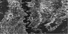
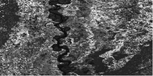
(CPU-Time, Relative-Error, PSNR)	(1136.81s, 0.0358, 37.85db)	(260.76s, 0.0374, 37.47db)	(246.17s, 0.0380, 37.32db)
(CPU-Time, Relative-Error, PSNR)	(586.05s, 0.0436, 36.27db)	(142.57s, 0.0455, 35.88db)	(122.92s, 0.0463, 35.74db)
(I) Original	(II) Truncated T-SVD [58]	(III) Proposed R-TSVD	(IV) Proposed RB-TSVD

Figure 1: Examples of large-scale high-order tensor approximation. From top to bottom are multi-temporal remote sensing images ($4500\times 4500\times 6\times 11$), color video ($1080\times 1920\times 3\times 500$), and light field images ($1152\times 1536\times 3\times 17\times 17$), respectively. (I) Original versions; (II)-(IV) The approximated version obtained by truncated T-SVD, R-TSVD, RB-TSVD, respectively.

III notations and preliminaries

For brevity, the main notations and preliminaries utilized in the whole paper are summarized in Table I, most of which originate form the literature [58].

In this work, we let ${\mathfrak{L}}(\boldsymbol{\mathcal{A}})$ represent the result of invertible linear transforms $\mathfrak{L}$ on $\boldsymbol{\mathcal{A}}\in\mathbb{R}^{n_{1}\times\cdots\times n_{d}}$, i.e.,

$$\mathfrak{L}(\boldsymbol{\mathcal{A}})=\boldsymbol{\mathcal{A}}\;{\times}_{3}\;\bm{U}_{n_{3}}\;{\times}_{4}\;\bm{U}_{n_{4}}\cdots{\times}_{d}\;\bm{U}_{n_{d}},$$ (2)

where the transform matrices $\bm{U}_{n_{i}}\in\mathbb{C}^{n_{i}\times n_{i}}$ of $\mathfrak{L}$ satisfies:

$${{\bm{U}}}_{n_{i}}\cdot{{\bm{U}}}^{\mit{H}}_{n_{i}}={{\bm{U}}}^{\mit{H}}_{n_{i}}\cdot{{\bm{U}}}_{n_{i}}=\alpha_{i}{{\bm{I}}}_{n_{i}},\forall i\in\{3,\cdots,d\},$$ (3)

in which $\alpha_{i}>0$ is a constant. The inverse operator of $\mathfrak{L}(\boldsymbol{\mathcal{A}})$ is defined as $\mathfrak{L}^{-1}(\boldsymbol{\mathcal{A}})=\boldsymbol{\mathcal{A}}\;{\times}_{d}\;\bm{U}^{-1}_{n_{d}}\;{\times}_{{d-1}}\;{{\bm{U}}_{n}}_{d-1}^{-1}\cdots{\times}_{3}\;\bm{U}^{-1}_{n_{3}}$, and $\mathfrak{L}^{-1}(\mathfrak{L}(\boldsymbol{\mathcal{A}}))=\boldsymbol{\mathcal{A}}$.

Definition III.1.

(Order-$d$ WTSN) Let $\mathfrak{L}$ be any invertible linear transform in (2) and it satisfies (3), ${\boldsymbol{\mathcal{S}}}$ be from the middle component of ${\boldsymbol{\mathcal{A}}}={\boldsymbol{\mathcal{U}}}{{*}_{\mathfrak{L}}}{\boldsymbol{\mathcal{S}}}{*}_{\mathfrak{L}}{\boldsymbol{\mathcal{V}}}^{\mit{T}}$. Then, the weighted tensor Schatten-$p$ norm (WTSN) of ${\boldsymbol{\mathcal{A}}}\in\mathbb{R}^{n_{1}\times\cdots\times n_{d}}$ is defined as

$$\|{\boldsymbol{\mathcal{A}}}\|_{{\boldsymbol{\mathcal{W}}},{\boldsymbol{\mathcal{S}}}_{p}} :={\Big{(}\frac{1}{\rho}\big{\|}\operatorname{bdiag}\big{(}{\mathfrak{L}}(\boldsymbol{\mathcal{A}})\big{)}\big{\|}_{{\bm{w}},{\mathrm{S}}_{p}}^{p}\Big{)}}^{1/p}$$

$$=\Big{(}\frac{1}{\rho}\sum_{j=1}^{n_{3}n_{4}\cdots n_{d}}\big{\|}{{\mathfrak{L}}(\boldsymbol{\mathcal{A}})}^{<j>}\big{\|}_{{{\bm{w}}^{(j)},{\mathrm{S}}_{p}}}^{p}\Big{)}^{{1}/{p}}$$

$$=\Big{(}\frac{1}{\rho}\sum_{j=1}^{n_{3}n_{4}\cdots n_{d}}\operatorname{trace}\big{(}{\boldsymbol{\mathcal{W}}}^{<j>}\cdot\big{|}{{\mathfrak{L}}({{\boldsymbol{\mathcal{S}}}})}^{<j>}\big{|}^{p}\big{)}\Big{)}^{{1}/{p}},$$

where $\boldsymbol{\mathcal{W}}$ is the nonnegative weight composed of an order-$d$ f-diagonal tensor, $\bm{w}=\operatorname{diag}(\operatorname{bdiag}(\boldsymbol{\mathcal{W}}))$, ${\bm{w}^{(j)}}=\operatorname{diag}(\boldsymbol{\mathcal{W}}^{<j>})$, and $\rho=\alpha_{3}\alpha_{4}\cdots\alpha_{d}>0$ is a constant determined by the invertible linear transform $\mathfrak{L}$.

Remark III.1.

The high-order WTSN (HWTSN) assigns different weight values to different singular values in the transform domain: the larger one is multiplied by a smaller weight while the smaller one is multiplied by a larger weight. That is, the weight values should be inversely proportional to the singular values in the transform domain. In particular, the HWTSN 1) is equivalent to the high-order tensor Schatten-$p$ norm (HTSN) when weighting is not taken into account, 2) reduces to the high-order weighted TNN (HWTNN)[61] when $p=1$, and 3) simplifies to the high-order TNN (HTNN)[58] when $p=1$, and $\boldsymbol{\mathcal{W}}$ is not considered.

Theorem III.1.

(Optimal $k$-term approximation [58]) Let the T-SVD of ${\boldsymbol{\mathcal{A}}}\in\mathbb{R}^{n_{1}\times\cdots\times n_{d}}$ be ${\boldsymbol{\mathcal{A}}}={\boldsymbol{\mathcal{U}}}{*}_{\mathfrak{L}}{\boldsymbol{\mathcal{S}}}{*}_{\mathfrak{L}}{\boldsymbol{\mathcal{V}}}^{\mit{T}}$ and define ${\boldsymbol{\mathcal{A}}}_{k}={\sum}_{i=1}^{k}{\boldsymbol{\mathcal{U}}}(:,i,:,\cdots,:){*}_{\mathfrak{L}}{\boldsymbol{\mathcal{S}}}(i,i,:,\cdots,:){*}_{\mathfrak{L}}{\boldsymbol{\mathcal{V}}}(:,i,:,\cdots,:)^{\mit{T}}$ for some $k<\min(n_{1},n_{2})$. Then, ${\boldsymbol{\mathcal{A}}}_{k}=\arg\min_{{\tilde{\boldsymbol{{\mathcal{A}}}}}\in\bm{\Theta}}\|{\boldsymbol{\mathcal{A}}}-{\tilde{\boldsymbol{{\mathcal{A}}}}}\|_{\mathnormal{F}}$, where $\bm{\Theta}=\{{\boldsymbol{\mathcal{X}}}{*}_{\mathfrak{L}}{\boldsymbol{\mathcal{Y}}}|{\boldsymbol{\mathcal{X}}}\in\mathbb{R}^{n_{1}\times k\times n_{3}\times\cdots\times n_{d}},{\boldsymbol{\mathcal{Y}}}\in\mathbb{R}^{k\times n_{2}\times n_{3}\times\cdots\times n_{d}}\}$. This implies that ${\boldsymbol{\mathcal{A}}}_{k}$ is the approximation of ${\boldsymbol{\mathcal{A}}}$ with the T-SVD rank at most $k$.

IV Randomized Techniques Based High-Order Tensor Approximation

The optimal $k$-term approximation presented in Theorem III.1 is time-consuming for large-scale tensors. To tackle this issue, an efficient QB approximation for high-order tensor is developed in virtue of randomized projection techniques. On this basis, we put forward an effective randomized algorithm for calculating the high-order T-SVD (abbreviated as R-TSVD). To be slightly more specific, the calculation of R-TSVD can be subdivided into the following two steps:

Input: $\bm{\mathcal{A}}\in\mathbb{R}^{n_{1}\times\cdots\times n_{d}}$, invertible linear transform: $\mathfrak{L}$, target T-SVD rank: $k$, oversampling parameter: $s$.

Output: $\bm{\mathcal{Q}},\bm{\mathcal{B}}$.

1 Set $\hat{l}=k+s$, and generate a Gaussian random tensor $\bm{\mathcal{G}}\in\mathbb{R}^{n_{2}\times\hat{l}\times n_{3}\times\cdots\times n_{d}}$;

2

3Construct a random projection of $\bm{\mathcal{A}}$ as ${\boldsymbol{\mathcal{Y}}}={\boldsymbol{\mathcal{A}}}{*}_{\mathfrak{L}}{\boldsymbol{\mathcal{G}}}$;

4

5Form the partially orthogonal tensor ${{\boldsymbol{\mathcal{Q}}}}$ by computing the T-QR factorization of $\bm{\mathcal{Y}}$;

6

${{\boldsymbol{\mathcal{B}}}}={\boldsymbol{\mathcal{Q}}}^{\mit{T}}{*}_{\mathfrak{L}}{{\boldsymbol{\mathcal{A}}}}$ .

Algorithm 1 The Basic randQB Approximation.

• Step I (Randomized Step): Compute an approximate basis for the range of the target tensor $\bm{\mathcal{A}}\in\mathbb{R}^{n_{1}\times n_{2}\times n_{3}\times\cdots\times n_{d}}$ via randomized projection techniques. That is to say, we require an orthogonal subspace basis tensor $\bm{\mathcal{Q}}\in\mathbb{R}^{n_{1}\times l\times n_{3}\times\cdots\times n_{d}}$ which satisfies

  $${\boldsymbol{\mathcal{A}}}\approx{\boldsymbol{\mathcal{Q}}}{*}_{\mathfrak{L}}{\boldsymbol{\mathcal{B}}}={\boldsymbol{\mathcal{Q}}}{*}_{\mathfrak{L}}{{\boldsymbol{\mathcal{Q}}}}^{\mit{T}}{*}_{\mathfrak{L}}{\boldsymbol{\mathcal{A}}}.$$ (4)

  The approximation presented by (4) can also be regarded as a kind of low-rank factorization/approximation of ${\boldsymbol{\mathcal{A}}}$, called QB factorization or QB approximation in our work. A basic randomized technique for computing the QB factorization is shown in Algorithm 1, which is denoted as the basic randomized QB (randQB) approximation.

• Step II (Deterministic Step): Perform the deterministic T-QR factorization on the reduced tensor ${\boldsymbol{\mathcal{B}}}^{\mit{T}}$, i.e., ${\boldsymbol{\mathcal{B}}}^{\mit{T}}={\boldsymbol{\mathcal{Q}}}_{1}{*}_{\mathfrak{L}}{\boldsymbol{\mathcal{R}}}$. Then, execute the deterministic T-SVD on the smaller tensor ${\boldsymbol{\mathcal{R}}}$, i.e., ${\boldsymbol{\mathcal{R}}}=\hat{{\boldsymbol{\mathcal{U}}}}{*}_{\mathfrak{L}}{\boldsymbol{\mathcal{S}}}{*}_{\mathfrak{L}}{\hat{{\boldsymbol{\mathcal{V}}}}}^{\mit{T}}$. Thus,

  $${\boldsymbol{\mathcal{A}}} \approx{\boldsymbol{\mathcal{Q}}}{*}_{\mathfrak{L}}\hat{{\boldsymbol{\mathcal{V}}}}{*}_{\mathfrak{L}}{\boldsymbol{\mathcal{S}}}{*}_{\mathfrak{L}}{\hat{\boldsymbol{\mathcal{U}}}}^{\mit{T}}{*}_{\mathfrak{L}}{{\boldsymbol{\mathcal{Q}}}_{1}}^{\mit{T}}$$

  $$={\boldsymbol{\mathcal{U}}}{*}_{\mathfrak{L}}{{\boldsymbol{\mathcal{S}}}}{*}_{\mathfrak{L}}{{\boldsymbol{\mathcal{V}}}}^{\mit{T}}(\textit{Let}\;{{\boldsymbol{\mathcal{U}}}}={{\boldsymbol{\mathcal{Q}}}}{*}_{\mathfrak{L}}\hat{{\boldsymbol{\mathcal{V}}}},{{\boldsymbol{\mathcal{V}}}}={{\boldsymbol{\mathcal{Q}}}_{1}}{*}_{\mathfrak{L}}\hat{{\boldsymbol{\mathcal{U}}}}).$$ (5)

Input: $\bm{\mathcal{A}}\in\mathbb{R}^{n_{1}\times\cdots\times n_{d}}$, transform: $\mathfrak{L}$, target T-SVD rank: $k$, oversampling parameter: $s$, power iteration: $t$.

Output: $\bm{\mathcal{U}}$, $\bm{\mathcal{S}}$, $\bm{\mathcal{V}}$.

1

2Set $\hat{l}=k+s$ and initialize a Gaussian random tensor $\bm{\mathcal{G}}\in\mathbb{R}^{n_{2}\times\hat{l}\times n_{3}\times\cdots\times n_{d}}$;

3

4Compute the results of $\mathfrak{L}$ on $\boldsymbol{\mathcal{A}}$ and $\boldsymbol{\mathcal{G}}$, i.e., $\mathfrak{L}(\boldsymbol{\mathcal{A}}),\mathfrak{L}(\boldsymbol{\mathcal{G}})$;

5

6for $v=1,2,\cdots,n_{3}\cdots n_{d}$ do

7      

8      $[\mathfrak{L}(\boldsymbol{\mathcal{Q}})^{<v>},\sim]=\operatorname{qr}(\mathfrak{L}(\boldsymbol{\mathcal{A}})^{<v>}\cdot\mathfrak{L}(\boldsymbol{\mathcal{G}})^{<v>})$;

9      

10      for $j=1,2,\ldots,t$ do

11             $[\mathfrak{L}(\boldsymbol{\mathcal{Q}}_{1})^{<v>},\sim]=\operatorname{qr}\big{(}{(\mathfrak{L}(\boldsymbol{\mathcal{A}})^{<v>})}^{\mit{T}}\cdot\mathfrak{L}(\boldsymbol{\mathcal{Q}})^{<v>}\big{)}$;

12             $[\mathfrak{L}(\boldsymbol{\mathcal{Q}})^{<v>},\sim]=\operatorname{qr}\big{(}\mathfrak{L}(\boldsymbol{\mathcal{A}})^{<v>}\cdot\mathfrak{L}(\boldsymbol{\mathcal{Q}}_{1})^{<v>}\big{)}$;

13            

14       end for

15      

16      $[\mathfrak{L}(\boldsymbol{\mathcal{Q}}_{1})^{<v>},\mathfrak{L}(\boldsymbol{\mathcal{R}})^{<v>}]=\textrm{qr}\big{(}(\mathfrak{L}(\boldsymbol{\mathcal{A}})^{<v>})^{\mit{T}}\cdot\mathfrak{L}(\boldsymbol{\mathcal{Q}})^{<v>}\big{)}$;

17      

18      $[\mathfrak{L}(\hat{\boldsymbol{\mathcal{U}}})^{<v>},\mathfrak{L}(\boldsymbol{\mathcal{S}})^{<v>},\mathfrak{L}(\hat{\boldsymbol{\mathcal{V}}})^{<v>}]=\textrm{svd}\big{(}\mathfrak{L}(\boldsymbol{\mathcal{R}})^{<v>}\big{)}$;

19      

20      $\mathfrak{L}(\boldsymbol{\mathcal{V}})^{<v>}=\mathfrak{L}(\boldsymbol{\mathcal{Q}}_{1})^{<v>}\cdot\mathfrak{L}(\hat{\boldsymbol{\mathcal{U}}})^{<v>}$;

21      

22      $\mathfrak{L}(\boldsymbol{\mathcal{U}})^{<v>}=\mathfrak{L}(\boldsymbol{\mathcal{Q}})^{<v>}\cdot\mathfrak{L}(\hat{\boldsymbol{\mathcal{V}}})^{<v>}$;

23      

24 end for

${\boldsymbol{\mathcal{U}}}\leftarrow{\mathfrak{L}}^{-1}({\mathfrak{L}}({\boldsymbol{\mathcal{U}}}))$, ${\boldsymbol{\mathcal{S}}}\leftarrow{\mathfrak{L}}^{-1}({\mathfrak{L}}({\boldsymbol{\mathcal{S}}}))$, ${\boldsymbol{\mathcal{V}}}\leftarrow{\mathfrak{L}}^{-1}({\mathfrak{L}}({\boldsymbol{\mathcal{V}}}))$.

Algorithm 2 Transform Domain Version: R-TSVD.

Remark IV.1.

(Power Iteration Strategy) To further improve the accuracy of randQB approximation of ${{\boldsymbol{\mathcal{A}}}}$, we can additionally apply the power iteration scheme, which multiplies alternately with ${{\boldsymbol{\mathcal{A}}}}$ and ${{{\boldsymbol{\mathcal{A}}}}}^{\mit{T}}$, i.e., ${({{\boldsymbol{\mathcal{A}}}}{*}_{\mathfrak{L}}{{{\boldsymbol{\mathcal{A}}}}}^{\mit{T}})}^{t}{*}_{\mathfrak{L}}{{\boldsymbol{\mathcal{A}}}}$, where $t$ is a nonnegative integer. Besides, to avoid the rounding error of float point arithmetic obtained from performing the power iteration, the reorthogonalization step is required. Thus, the randQB approximation algorithm incorporating power iteration strategy can be obtained by adding the following steps after the third step of Algorithm 1, i.e.,

for $j=1,2,\ldots,t$ do

       $[{{\boldsymbol{\mathcal{Q}}}_{1}},\sim]=\operatorname{H-TQR}({\boldsymbol{\mathcal{A}}}^{\mit{T}}{*}_{\mathfrak{L}}{{\boldsymbol{\mathcal{Q}}}},\mathfrak{L})$;  $[{{\boldsymbol{\mathcal{Q}}}},\sim]=\operatorname{H-TQR}({\boldsymbol{\mathcal{A}}}{*}_{\mathfrak{L}}{{\boldsymbol{\mathcal{Q}}}_{1}},\mathfrak{L})$; 

end for

Input: $\bm{\mathcal{A}}\in\mathbb{R}^{n_{1}\times\cdots\times n_{d}}$, transform: $\mathfrak{L}$, target T-SVD Rank: $k$, block size: $b$, power iteration: $t$. Output: $\bm{\mathcal{U}}$, $\bm{\mathcal{S}}$, $\bm{\mathcal{V}}$. 1 2Let $\hat{l}$ be a number slightly larger than $k$, and generate a Gaussian random tensor $\bm{\mathcal{G}}\in\mathbb{R}^{n_{2}\times\hat{l}\times n_{3}\times\cdots\times n_{d}}$; 3 4Compute the results of $\mathfrak{L}$ on $\boldsymbol{\mathcal{A}}$ and $\boldsymbol{\mathcal{G}}$, i.e., $\mathfrak{L}(\boldsymbol{\mathcal{A}}),\mathfrak{L}(\boldsymbol{\mathcal{G}})$; 5 6for $v=1,2,\cdots,n_{3}\cdots n_{d}$ do 7       8      ${\mathfrak{L}(\boldsymbol{\mathcal{Q}})}^{<v>}=[\;\;];\;\;{\mathfrak{L}(\boldsymbol{\mathcal{B}})}^{<v>}=[\;\;]$; 9       10      for $j=1,2,\ldots,t$ do 11             $[\mathfrak{L}(\boldsymbol{\mathcal{W}})^{<v>},\sim]=\operatorname{qr}(\mathfrak{L}(\boldsymbol{\mathcal{A}})^{<v>}\cdot\mathfrak{L}(\boldsymbol{\mathcal{G}})^{<v>})$; 12             $[\mathfrak{L}(\boldsymbol{\mathcal{G}})^{<v>},\sim]=\operatorname{qr}\big{(}{(\mathfrak{L}(\boldsymbol{\mathcal{A}})^{<v>})}^{\mit{T}}\cdot\mathfrak{L}(\boldsymbol{\mathcal{W}})^{<v>}\big{)}$; 13             14       end for 15       16      $\mathfrak{L}(\boldsymbol{\mathcal{W}})^{<v>}=\mathfrak{L}(\boldsymbol{\mathcal{A}})^{<v>}\cdot\mathfrak{L}(\boldsymbol{\mathcal{G}})^{<v>}$ ; 17       18      $\mathfrak{L}(\boldsymbol{\mathcal{H}})^{<v>}={(\mathfrak{L}(\boldsymbol{\mathcal{A}})^{<v>})}^{\mit{T}}\cdot\mathfrak{L}(\boldsymbol{\mathcal{W}})^{<v>}$; 19       20      for $i=1,2,\cdots,\lfloor\frac{\hat{l}}{b}\rfloor$ do 21             $\mathfrak{L}\big{(}{\boldsymbol{\mathcal{G}}}^{(i)}\big{)}^{<v>}=\mathfrak{L}(\boldsymbol{\mathcal{G}})^{<v>}\big{(}:,(i-1)b+1:ib\big{)}$; 22             23            $\mathfrak{L}\big{(}{\boldsymbol{\mathcal{Y}}}^{(i)}\big{)}^{<v>}=-\mathfrak{L}(\boldsymbol{\mathcal{Q}})^{<v>}\cdot\mathfrak{L}(\boldsymbol{\mathcal{B}})^{<v>}\cdot\mathfrak{L}({\boldsymbol{\mathcal{G}}}^{(i)})^{<v>}+\mathfrak{L}(\boldsymbol{\mathcal{W}})^{<v>}\big{(}:,(i-1)b+1:ib\big{)}$ ; 24             25            $[{\mathfrak{L}({\boldsymbol{\mathcal{Q}}}^{(i)})}^{<v>},\mathfrak{L}({\boldsymbol{\mathcal{R}}}^{(i)})^{<v>}]=\operatorname{qr}\big{(}\mathfrak{L}({\boldsymbol{\mathcal{Y}}}^{(i)})^{<v>}\big{)}$; 26             27            $[{\mathfrak{L}({\boldsymbol{\mathcal{Q}}}^{(i)})}^{<v>},{(\mathfrak{L}({\hat{\boldsymbol{\mathcal{R}}}}^{(i)}))}^{<v>}]=\operatorname{qr}({\mathfrak{L}({\boldsymbol{\mathcal{Q}}}^{(i)})}^{<v>}-{\mathfrak{L}({\boldsymbol{\mathcal{Q}}})}^{<v>}\cdot{(\mathfrak{L}(\boldsymbol{\mathcal{Q}})^{<v>})}^{\mit{T}}\cdot{\mathfrak{L}({\boldsymbol{\mathcal{Q}}}^{(i)})}^{<v>})$; 28             29            ${\mathfrak{L}({\boldsymbol{\mathcal{R}}}^{(i)})}^{<v>}={(\mathfrak{L}({\hat{\boldsymbol{\mathcal{R}}}}^{(i)}))}^{<v>}\cdot{\mathfrak{L}({\boldsymbol{\mathcal{R}}}^{(i)})}^{<v>}$; 30             31            ${\mathfrak{L}({\boldsymbol{\mathcal{B}}}^{(i)})}^{<v>}={\big{(}\mathfrak{L}({{\boldsymbol{\mathcal{R}}}^{(i)}})^{<v>}\big{)}}^{\mit{-T}}\cdot\big{[}{\big{(}{\mathfrak{L}({\boldsymbol{\mathcal{H}}})}^{<v>}(:,(i-1)b+1:ib)\big{)}}^{\mit{T}}-{({\mathfrak{L}({\boldsymbol{\mathcal{Y}}}^{(i)})}^{<v>})}^{\mit{T}}\cdot{\mathfrak{L}({\boldsymbol{\mathcal{Q}}})}^{<v>}\cdot{\mathfrak{L}({\boldsymbol{\mathcal{B}}})}^{<v>}-{({\mathfrak{L}({\boldsymbol{\mathcal{G}}}^{(i)})}^{<v>})}^{\mit{T}}\cdot{(\mathfrak{L}(\boldsymbol{\mathcal{B}})^{<v>})}^{\mit{T}}\cdot{\mathfrak{L}({\boldsymbol{\mathcal{B}}})}^{<v>}\big{]}$; 32             33            $\mathfrak{L}(\boldsymbol{\mathcal{Q}})^{<v>}=[\mathfrak{L}(\boldsymbol{\mathcal{Q}})^{<v>},{\mathfrak{L}({\boldsymbol{\mathcal{Q}}}^{(i)})}^{<v>}]$; 34             $\mathfrak{L}(\boldsymbol{\mathcal{B}})^{<v>}=[\mathfrak{L}(\boldsymbol{\mathcal{B}})^{<v>},{\mathfrak{L}({\boldsymbol{\mathcal{B}}}^{(i)})}^{<v>}]^{\mit{T}}$; 35             36       end for 37       38      $[\mathfrak{L}(\boldsymbol{\mathcal{Q}}_{1})^{<v>},\mathfrak{L}(\boldsymbol{\mathcal{R}}_{1})^{<v>}]=\textrm{qr}\big{(}(\mathfrak{L}(\boldsymbol{\mathcal{B}})^{<v>})^{\mit{T}}\big{)}$; 39       40      $[\mathfrak{L}(\hat{\boldsymbol{\mathcal{U}}})^{<v>},\mathfrak{L}(\boldsymbol{\mathcal{S}})^{<v>},\mathfrak{L}(\hat{\boldsymbol{\mathcal{V}}})^{<v>}]=\textrm{svd}\big{(}\mathfrak{L}(\boldsymbol{\mathcal{R}}_{1})^{<v>}\big{)}$; 41       42      $\mathfrak{L}(\boldsymbol{\mathcal{V}})^{<v>}=\mathfrak{L}(\boldsymbol{\mathcal{Q}}_{1})^{<v>}\cdot\mathfrak{L}(\hat{\boldsymbol{\mathcal{U}}})^{<v>}$; 43       44      $\mathfrak{L}(\boldsymbol{\mathcal{U}})^{<v>}=\mathfrak{L}(\boldsymbol{\mathcal{Q}})^{<v>}\cdot\mathfrak{L}(\hat{\boldsymbol{\mathcal{V}}})^{<v>}$; 45       46 end for ${\boldsymbol{\mathcal{U}}}\leftarrow{\mathfrak{L}}^{-1}({\mathfrak{L}}({\boldsymbol{\mathcal{U}}}))$, ${\boldsymbol{\mathcal{S}}}\leftarrow{\mathfrak{L}}^{-1}({\mathfrak{L}}({\boldsymbol{\mathcal{S}}}))$, ${\boldsymbol{\mathcal{V}}}\leftarrow{\mathfrak{L}}^{-1}({\mathfrak{L}}({\boldsymbol{\mathcal{V}}}))$. Algorithm 3 Transform Domain Version: RB-TSVD. According to the above analysis, the computational procedure of R-TSVD is shown in Algorithm 2. To obtain high performance of linear algebraic computation, we further investigate the blocked version of basic randQB approximation, and then derive a randomized blocked algorithm for computing high-order T-SVD (abbreviated as RB-TSVD, see Algorithm 3). Owing to the space limitations of this paper, the detailed derivation of blocked randQB approximation and its induced RB-TSVD are given in the supplementary material. The experimental results shown in Figure 1 indicate that for various real-world large-scale tensors, the proposed RB-TSVD and R-TSVD algorithms achieve up to $4$$\sim$$8$X faster running time than the previous truncated T-SVD while maintaining similar accuracy. Besides, there is no significant difference between RB-TSVD and R-TSVD in calculation time. Only for very large-scale tensors (i.e., the spatial dimensions up to about $10^{4}\times 10^{4}$) does the advantage of RB-TSVD show up, which is verified in the supplementary materials.

V Rubust High-Order Tensor Completion

V-A Proposed Model

In this subsection, we formally introduce the double nonconvex model for RHTC, in which the low-rank component is constrained by the HWTSN (see Definition III.1), while the noise/outlier component is regularized by its weighted $\ell_{q}$-norm (see Table I). Specifically, suppose that we are given a low T-SVD rank tensor ${\boldsymbol{\mathcal{L}}}\in\mathbb{R}^{n_{1}\times\cdots\times n_{d}}$ corrupted by the noise or outliers. The corrupted part can be represented by the tensor ${\boldsymbol{\mathcal{E}}}\in\mathbb{R}^{n_{1}\times\cdots\times n_{d}}$. Here, both ${\boldsymbol{\mathcal{L}}}$ and ${\boldsymbol{\mathcal{E}}}$ are of arbitrary magnitude. We do not know the T-SVD rank of ${\boldsymbol{\mathcal{L}}}$. Moreover, we have no idea about the locations of the nonzero entries of ${\boldsymbol{\mathcal{E}}}$, not even how many there are. Then, the goal of the RHTC problem is to achieve the reconstruction (either exactly or approximately) of low-rank component ${\boldsymbol{\mathcal{L}}}$ from an observed subset of corrupted tensor ${\boldsymbol{\mathcal{M}}}={\boldsymbol{\mathcal{L}}}+{\boldsymbol{\mathcal{E}}}$. Mathematically, the proposed RHTC model can be formulated as follows: $$\min_{{\boldsymbol{\mathcal{L}}},{\boldsymbol{\mathcal{E}}}}\|{\boldsymbol{\mathcal{L}}}\|_{{{\boldsymbol{\mathcal{W}}}_{1},{\boldsymbol{\mathcal{S}}}_{p}}}^{p}+\lambda\|{\boldsymbol{\mathcal{E}}}\|_{{\boldsymbol{\mathcal{W}}}_{2},\ell_{q}}^{q},\boldsymbol{\bm{P}}_{{{\Omega}}}({\boldsymbol{\mathcal{L}}}+{\boldsymbol{\mathcal{E}}})=\boldsymbol{\bm{P}}_{{{\Omega}}}({\boldsymbol{\mathcal{M}}}),$$ (6) where $0<p,q<1$, $\lambda>0$ is the penalty parameter, $\|{\boldsymbol{\mathcal{L}}}\|_{{{\boldsymbol{\mathcal{W}}}_{1},{\boldsymbol{\mathcal{S}}}_{p}}}$ denotes the HWTSN of ${\boldsymbol{\mathcal{L}}}$ while $\|{\boldsymbol{\mathcal{E}}}\|_{{\boldsymbol{\mathcal{W}}}_{2},\ell_{q}}$ represents the weighted $\ell_{q}$-norm of ${\boldsymbol{\mathcal{E}}}$, and ${\boldsymbol{\mathcal{W}}}_{1}$ and ${\boldsymbol{\mathcal{W}}}_{2}$ are the weight tensors, which will be updated automatically in the subsequent ADMM optimization, see V-C for details.

Remark V.1.

In the model (6), the HWTSN not only gives better approximation to the original low-rank assumption, but also considers the importance of different singular components. Comparing with the previous regularizers, e.g., HWTNN and HTNN/HTSN (treat the different rank components equally), the proposed one is tighter and more feasible. Besides, the weighted $\ell_{q}$-norm has a superior potential to be sparsity-promoting in comparison with the $\ell_{1}$-norm and $\ell_{q}$-norm. Therefore, the joint HWTSN and weighted $\ell_{q}$-norm enables the underlying low-rank structure in the observed tensor ${\boldsymbol{\mathcal{M}}}$ to be well captured, and the robustness against noise/outliers to be well enhanced. The proposed two nonconvex regularizers mainly involve several key ingredients: 1) flexible linear transforms $\mathfrak{L}$; 2) adjustable parameters $p$ and $q$; 3) automatically updated weight tensors ${\boldsymbol{\mathcal{W}}}_{1}$ and ${\boldsymbol{\mathcal{W}}}_{2}$. Their various combinations can degenerate to many existing RLRTC models.

V-B HWTSN Minimization Problem

In this subsection, we mainly present the solution method of HWTSN minimization problem, that is, the method of solving $\displaystyle\arg\min_{{\boldsymbol{\mathcal{X}}}}\tau\|{\boldsymbol{\mathcal{X}}}\|_{{{\boldsymbol{\mathcal{W}}},{\boldsymbol{\mathcal{S}}}_{p}}}^{p}+\frac{1}{2}\|{\boldsymbol{\mathcal{X}}}-{\boldsymbol{\mathcal{Z}}}\|^{2}_{\mathnormal{F}}.$ (7) Before providing the solution to problem (7), we first introduce the key lemma and definition.

Lemma V.1.

[77] For the given $p$ ($0<p<1$) and $w>0$, the optimal solution of the following optimization problem $$\min_{x}w|x|^{p}+\frac{1}{2}{(x-s)}^{2}$$ (8) is given by the generalized soft-thresholding (GST) operator: $\displaystyle\hat{x}=\operatorname{{{GST}}}\big{(}s,w,p\big{)}=\begin{cases}0,\;\;\;\;\;\;\;\;\;\;\;\;\;\;\;\;\;\;\;\;\;\;\;\;\;\;\;\text{if}\;|s|\leq\delta,\\ \operatorname{sign}(s){\hat{\alpha}}^{*}\;\;\;\;\;\;\;\;\;\;\;\;\;\;\;\;\text{if}\;|s|>\delta,\end{cases}$ where $\delta={[2w(1-p)]}^{\frac{1}{2-p}}+wp{[2w(1-p)]}^{\frac{p-1}{2-p}}$ is a threshold value, $\operatorname{sign}(s)$ denotes the signum function, and ${\hat{\alpha}}^{*}$ can be obtained by solving ${\alpha}+wp{\alpha}^{p-1}-|s|=0\;(\alpha>0)$.

Definition V.1.

(GTSVT operator) Let ${\boldsymbol{\mathcal{A}}}={\boldsymbol{\mathcal{U}}}{*}_{\mathfrak{L}}{\boldsymbol{\mathcal{S}}}{*}_{\mathfrak{L}}{\boldsymbol{\mathcal{V}}}^{\mit{T}}$ be the T-SVD of ${\boldsymbol{\mathcal{A}}}\in\mathbb{R}^{n_{1}\times\cdots\times n_{d}}$. For any $\tau>0$, $0<p<1$, then the generalized Tensor Singular Value Thresholding (GTSVT) operator of ${\boldsymbol{\mathcal{A}}}$ is defined as follows $${\boldsymbol{\mathcal{D}}}_{{\boldsymbol{\mathcal{W}}},p,\tau}({\boldsymbol{\mathcal{A}}})={\boldsymbol{\mathcal{U}}}{*}_{\mathfrak{L}}{\boldsymbol{\mathcal{S}}}_{{\boldsymbol{\mathcal{W}}},p,\tau}{*}_{\mathfrak{L}}{\boldsymbol{\mathcal{V}}}^{\mit{T}},$$ (9) where ${\boldsymbol{\mathcal{S}}}_{{\boldsymbol{\mathcal{W}}},p,\tau}={\mathfrak{L}^{-1}}\big{(}GST({{\mathfrak{L}}({\boldsymbol{\mathcal{S}}})},\tau{\boldsymbol{\mathcal{W}}},p)\big{)}$, ${\boldsymbol{\mathcal{W}}}\in\mathbb{R}^{n_{1}\times\cdots\times n_{d}}$ is the weight parameter composed of an order-$d$ f-diagonal tensor, and $\operatorname{GST}$ denotes the element-wise shrinkage operator.

Remark V.2.

Since the larger singular values usually carry more important information than the smaller ones, the GTSVT operator requires to satisfy: the larger singular values in the transform domain should be shrunk less, while the smaller ones should be shrunk more. In other words, the weights are selected inversely to the singular values in the transform domain. Thus, the original components corresponding to the larger singular values will be less affected. The GTSVT operator is more flexible than the T-SVT operator proposed in [58] (shrinks all singular values with the same threshold) and the WTSVT operator proposed in [61], and provides more degree of freedom for the approximation to the original problem.

Theorem V.1.

Let $\mathfrak{L}$ be any invertible linear transform in (2) and it satisfies (3), $m=\min{(n_{1},n_{2})}$. For any $\tau>0$ and ${\boldsymbol{\mathcal{Z}}}\in\mathbb{R}^{n_{1}\times\cdots\times n_{d}}$, if the weight parameter satisfies $$0\leq{\boldsymbol{\mathcal{W}}}^{<j>}(1,1)\leq\cdots\leq{\boldsymbol{\mathcal{W}}}^{<j>}(m,m),\;\forall j\in[n_{3}\cdots n_{d}],$$ then the GTSVT operator (9) obeys $\displaystyle{\boldsymbol{\mathcal{D}}}_{{\boldsymbol{\mathcal{W}}},p,\tau}({\boldsymbol{\mathcal{Z}}})=\arg\min_{{\boldsymbol{\mathcal{X}}}}\tau\|{\boldsymbol{\mathcal{X}}}\|_{{{\boldsymbol{\mathcal{W}}},{\boldsymbol{\mathcal{S}}}_{p}}}^{p}+\frac{1}{2}\|{\boldsymbol{\mathcal{X}}}-{\boldsymbol{\mathcal{Z}}}\|^{2}_{\mathnormal{F}}.$ (10)

Proposition V.1.

Let ${{\boldsymbol{\mathcal{A}}}}={{\boldsymbol{\mathcal{Q}}}}{*}_{\mathfrak{L}}{\boldsymbol{\mathcal{B}}}\in\mathbb{R}^{n_{1}\times n_{2}\times\cdots\times n_{d}}$, where ${{\boldsymbol{\mathcal{Q}}}}\in\mathbb{R}^{n_{1}\times k\times\cdots\times n_{d}}$ is partially orthogonal and ${{\boldsymbol{\mathcal{B}}}}\in\mathbb{R}^{k\times n_{2}\times\cdots\times n_{d}}$. Then, we have $${\boldsymbol{\mathcal{D}}}_{{\boldsymbol{\mathcal{W}}},p,\tau}({\boldsymbol{\mathcal{A}}})={{\boldsymbol{\mathcal{Q}}}}{*}_{\mathfrak{L}}{\boldsymbol{\mathcal{D}}}_{{\boldsymbol{\mathcal{W}}},p,\tau}({\boldsymbol{\mathcal{B}}}).$$

Proposition V.2.

Let ${{\boldsymbol{\mathcal{A}}}}={{\boldsymbol{\mathcal{Q}}}_{1}}{*}_{\mathfrak{L}}{\boldsymbol{\mathcal{B}}}{*}_{\mathfrak{L}}{{\boldsymbol{\mathcal{Q}}}_{2}^{\mit{T}}}\in\mathbb{R}^{n_{1}\times n_{2}\times\cdots\times n_{d}}$, where ${{\boldsymbol{\mathcal{Q}}}_{1}}\in\mathbb{R}^{n_{1}\times k\times\cdots\times n_{d}}$ and ${{\boldsymbol{\mathcal{Q}}}_{2}}\in\mathbb{R}^{n_{2}\times k\times\cdots\times n_{d}}$ are partially orthogonal, ${{\boldsymbol{\mathcal{B}}}}\in\mathbb{R}^{k\times k\times\cdots\times n_{d}}$. Then, we have $${\boldsymbol{\mathcal{D}}}_{{\boldsymbol{\mathcal{W}}},p,\tau}({\boldsymbol{\mathcal{A}}})={{\boldsymbol{\mathcal{Q}}}_{1}}{*}_{\mathfrak{L}}{\boldsymbol{\mathcal{D}}}_{{\boldsymbol{\mathcal{W}}},p,\tau}({\boldsymbol{\mathcal{B}}}){*}_{\mathfrak{L}}{{\boldsymbol{\mathcal{Q}}}_{2}^{\mit{T}}}.$$

Remark V.3.

From the Definition V.1 and Theorem V.1, we can find that the major computational bottleneck of HWTSN minimization problem (7) is to execute the GTSVT operator involving T-SVD multiple times. Based on the previous Proposition V.1,V.2, we can avoid expensive computation by instead calculating GTSVT on a smaller tensor ${{\boldsymbol{\mathcal{B}}}}$. In other words, we can efficiently calculate GTSVT operator according to the following two steps: 1) compute two orthogonal subspace basis tensor $\bm{\mathcal{Q}}_{1},\bm{\mathcal{Q}}_{2}$ via random projection techniques; 2) perform the GTSVT operator on a smaller tensor ${{\boldsymbol{\mathcal{B}}}}$. The computational procedure of GTSVT is shown in Algorithm 5. What is particularly noteworthy is that the Algorithm 5 is highly parallelizable because the operations across frontal slices can be readily distributed across different processors. Therefore, additional computational gains can be achieved in virtue of the parallel computing framework. Input: $s,w,p,J=3$ or $4$. Output: $\operatorname{{{GST}}}\big{(}s,w,p\big{)}$. 1 2${{\delta}}^{GST}_{p}(w)={[2w(1-p)]}^{\frac{1}{2-p}}+wp{{[2w(1-p)]}^{\frac{p-1}{2-p}}}$; 3 if $|s|\leq{{\delta}}^{GST}_{p}(w)$ then 4       $\operatorname{{{GST}}}\big{(}s,w,p\big{)}=0$ ; 5       6else 7      $j=0,x^{(j)}=|s|$; 8       for $j=0,1,\cdots,J$ do 9             $x^{(j+1)}=|s|-wp(x^{(j)})^{p-1}$; 10             $j=j+1$; 11       end for 12      $\operatorname{{{GST}}}\big{(}s,w,p\big{)}=\operatorname{sgn}(s)x^{(j)}$; 13 end if Algorithm 4 GST algorithm [77]. Input: $\bm{\mathcal{A}}\in\mathbb{R}^{n_{1}\times\cdots\times n_{d}}$, transform: $\mathfrak{L}$, target T-SVD Rank: $k$, weight tensor: ${\boldsymbol{\mathcal{W}}}\in\mathbb{R}^{n_{1}\times\cdots\times n_{d}}$, block size: $b$, $0<p<1$, $\tau>0$, power iteration: $t$. 1 2Let $\hat{l}$ be a number slightly larger than $k$ and generate a Gaussian random tensor $\bm{\mathcal{G}}\in\mathbb{R}^{n_{2}\times\hat{l}\times n_{3}\times\cdots\times n_{d}}$; 3 4Compute the results of $\mathfrak{L}$ on $\boldsymbol{\mathcal{A}}$ and $\boldsymbol{\mathcal{G}}$, i.e., $\mathfrak{L}(\boldsymbol{\mathcal{A}}),\mathfrak{L}(\boldsymbol{\mathcal{G}})$; 5 6 for $v=1,2,\cdots,n_{3}n_{4}\cdots n_{d}$ do 7       8      if  utilize the unblocked randomized technique  then 9             Execute Lines 4-12 of Algorithm 2 to obtain ${\mathfrak{L}}({\boldsymbol{\mathcal{U}}})^{<v>}$, ${\mathfrak{L}}({\boldsymbol{\mathcal{S}}})^{<v>}$, and ${\mathfrak{L}}({\boldsymbol{\mathcal{V}}})^{<v>}$ ; 10             11       end if 12       13      else if  utilize the blocked randomized technique  then 14             Execute Lines 4-24 of Algorithm 3 to obtain ${\mathfrak{L}}({\boldsymbol{\mathcal{U}}})^{<v>}$, ${\mathfrak{L}}({\boldsymbol{\mathcal{S}}})^{<v>}$, and ${\mathfrak{L}}({\boldsymbol{\mathcal{V}}})^{<v>}$ ; 15             16       end if 17      else if  not utilize the randomized technique  then 18             $[{\mathfrak{L}}({\boldsymbol{\mathcal{U}}})^{<v>},{\mathfrak{L}}({\boldsymbol{\mathcal{S}}})^{<v>},{\mathfrak{L}}({\boldsymbol{\mathcal{V}}})^{<v>}]=\textrm{svd}\big{(}{\boldsymbol{\mathcal{A}}}_{\mathfrak{L}}^{<v>}\big{)}$ ; 19             20       end if 21       22      $\hat{\bm{S}}=\operatorname{{{GST}}}\big{\{}{\operatorname{diag}(\mathfrak{L}(\boldsymbol{\mathcal{S}})^{<v>})},\tau\cdot{\operatorname{diag}({{\boldsymbol{\mathcal{W}}}}^{<v>})},p\big{\}}$; 23       24      ${\mathfrak{L}(\boldsymbol{\mathcal{C}})}^{<v>}={\mathfrak{L}(\boldsymbol{\mathcal{U}})}^{<v>}\cdot\operatorname{diag}(\hat{\bm{S}})\cdot{(\mathfrak{L}(\boldsymbol{\mathcal{V}})^{<v>})}^{\mit{T}}$ ; 25       26 end for 27 28 29 Output: ${\boldsymbol{\mathcal{D}}}_{{\boldsymbol{\mathcal{W}}},p,\tau}({\boldsymbol{\mathcal{A}}},\mathfrak{L})\leftarrow{\mathfrak{L}}^{-1}({\mathfrak{L}}({\boldsymbol{\mathcal{C}}}))$ . 30 Algorithm 5 High-Order GTSVT, ${\boldsymbol{\mathcal{D}}}_{{\boldsymbol{\mathcal{W}}},p,\tau}({\boldsymbol{\mathcal{A}}},\mathfrak{L})$.

V-C Optimization Algorithm

In this subsection, the ADMM framework [78] is adopted to solve the proposed model (6). The nonconvex model (6) can be equivalently reformulated as follows: $$\min_{{\boldsymbol{\mathcal{L}}},{\boldsymbol{\mathcal{E}}}}\|{\boldsymbol{\mathcal{L}}}\|_{{{\boldsymbol{\mathcal{W}}}_{1},{\boldsymbol{\mathcal{S}}}_{p}}}^{p}+\lambda\|\boldsymbol{\bm{P}}_{{{\Omega}}}({\boldsymbol{\mathcal{E}}})\|_{{\boldsymbol{\mathcal{W}}}_{2},\ell_{q}}^{q},\;\;\text{s.t.}\;\;{\boldsymbol{\mathcal{L}}}+{\boldsymbol{\mathcal{E}}}={\boldsymbol{\mathcal{M}}}.$$ (11) The augmented Lagrangian function of (11) is $\displaystyle\mathcal{F}({\boldsymbol{\mathcal{L}}},{\boldsymbol{\mathcal{E}}},{\boldsymbol{\mathcal{Y}}},\beta)=\|{\boldsymbol{\mathcal{L}}}\|_{{{\boldsymbol{\mathcal{W}}}_{1},{\boldsymbol{\mathcal{S}}}_{p}}}^{p}+\lambda\|\boldsymbol{\bm{P}}_{{{\Omega}}}({\boldsymbol{\mathcal{E}}})\|_{{\boldsymbol{\mathcal{W}}}_{2},\ell_{q}}^{q}+$ $\displaystyle\langle{\boldsymbol{\mathcal{Y}}},{{\boldsymbol{\mathcal{L}}}+{\boldsymbol{\mathcal{E}}}-\boldsymbol{\mathcal{M}}}\rangle+{\beta}/{2}\|{\boldsymbol{\mathcal{L}}}+{\boldsymbol{\mathcal{E}}}-{\boldsymbol{\mathcal{M}}}\|^{2}_{{{\mathnormal{F}}}},$ (12) where ${\boldsymbol{\mathcal{Y}}}$ is the dual variable and $\beta$ is the regularization parameter. The ADMM framework alternately updates each optimization variable until convergence. The iteration template of the ADMM at the ($k+1$)-th iteration is described as follows: $\displaystyle{\boldsymbol{\mathcal{L}}}^{k+1}$ $\displaystyle=\arg\min_{\boldsymbol{\mathcal{L}}}\big{\{}\mathcal{F}({\boldsymbol{\mathcal{L}}},{\boldsymbol{\mathcal{E}}}^{k},{\boldsymbol{\mathcal{Y}}}^{k},\beta^{k})\big{\}},$ (13) $\displaystyle{\boldsymbol{\mathcal{E}}}^{k+1}$ $\displaystyle=\arg\min_{\boldsymbol{\mathcal{E}}}\;\big{\{}\mathcal{F}({\boldsymbol{\mathcal{L}}}^{k+1},{\boldsymbol{\mathcal{E}}},{\boldsymbol{\mathcal{Y}}}^{k},\beta^{k})\big{\}},$ (14) $\displaystyle{\boldsymbol{\mathcal{Y}}}^{k+1}$ $\displaystyle={\boldsymbol{\mathcal{Y}}}^{k}+\beta^{k}({\boldsymbol{\mathcal{L}}}^{k+1}+{\boldsymbol{\mathcal{E}}}^{k+1}-{\boldsymbol{\mathcal{M}}}),$ (15) $\displaystyle\beta^{k+1}$ $\displaystyle=\min\left(\beta^{\operatorname{max}},\vartheta\beta^{k}\right),$ (16) where $\vartheta>1$ is a control constant. Now we solve the subproblem (13) and (14) explicitly in the ADMM, respectively. Update ${\boldsymbol{\mathcal{L}}^{k+1}}$ (low-rank component) The optimization subproblem (13) concerning ${\boldsymbol{\mathcal{L}}^{k+1}}$ can be written as $\displaystyle\min_{\boldsymbol{\mathcal{L}}}\big{\|}{\boldsymbol{\mathcal{L}}}\big{\|}_{{{{{\boldsymbol{\mathcal{W}}}_{1}}^{k}},{\boldsymbol{\mathcal{S}}}_{p}}}^{p}+{\beta^{k}}/{2}\big{\|}{\boldsymbol{\mathcal{L}}}-{\boldsymbol{\mathcal{M}}}+{\boldsymbol{\mathcal{E}}}^{k}+{{\boldsymbol{\mathcal{Y}}}^{k}}/{\beta^{k}}\big{\|}^{2}_{\mathnormal{F}}.$ (17) Let ${\boldsymbol{\mathcal{G}}}^{k}={\boldsymbol{\mathcal{M}}}-{\boldsymbol{\mathcal{E}}}^{k}-{{\boldsymbol{\mathcal{Y}}}^{k}}/{\beta^{k}}$. Using the GTSVT algorithm that incorporates the randomized schemes, the subproblem (17) can be efficiently solved, i.e., ${\boldsymbol{\mathcal{L}}}^{k+1}={\boldsymbol{\mathcal{D}}}_{{{\boldsymbol{\mathcal{W}}}_{1}}^{k},p,\frac{1}{\beta^{k}}}({\boldsymbol{\mathcal{G}}}^{k},\mathfrak{L})$.

Remark V.4.

(Update ${{\boldsymbol{\mathcal{W}}}_{1}}$ via reweighting strategy) The weight tensor ${\boldsymbol{\mathcal{W}}_{1}}$ can be adaptively tuned at each iteration, and its formula in the $k$-th iteration is given by $${({\boldsymbol{\mathcal{W}}_{1}}^{k})}^{<j>}(i,i)={\frac{c_{1}}{{{({{\boldsymbol{\mathcal{K}}}^{k}})}^{<j>}(i,i)+\epsilon_{1}}}}\cdot\frac{1}{\beta^{k}},\;$$ where $j\in\{1,\cdots,n_{3}\cdots n_{d}\}$, $i\in\{1,\cdots,\min(n_{1},n_{2})\}$, $c_{1}>0$ is a constant, $\epsilon_{1}$ is a small non-negative constant to avoid division by zero, and the entries on the diagonal of ${({{{\boldsymbol{\mathcal{K}}}}^{k}})}^{<j>}$ represent the singular values of ${{{\mathfrak{L}}({\boldsymbol{\mathcal{G}}}^{k})}}^{<j>}$. In such a reweighted technique, the sparsity performance is enhanced after each iteration and the updated ${{\boldsymbol{\mathcal{W}}}_{1}}^{k}$ satisfy: $${({\boldsymbol{\mathcal{W}}_{1}}^{k})}^{<j>}(m,m)\geq{({\boldsymbol{\mathcal{W}}_{1}}^{k})}^{<j>}(n,n)\geq 0,\;\forall m\geq n.$$ Update ${\boldsymbol{\mathcal{E}}^{k+1}}$ (noise/outliers component) The optimization subproblem (14) with respect to $\boldsymbol{\mathcal{E}}^{k+1}$ can be written as $\displaystyle\min_{\boldsymbol{\mathcal{E}}}\lambda\|\boldsymbol{\bm{P}}_{{{\Omega}}}({\boldsymbol{\mathcal{E}}})\|_{{{\boldsymbol{\mathcal{W}}}_{2}}^{k},\ell_{q}}^{q}+{\beta^{k}}/{2}\big{\|}{\boldsymbol{\mathcal{E}}}-{\boldsymbol{\mathcal{M}}}+{\boldsymbol{\mathcal{L}}}^{k+1}+{{\boldsymbol{\mathcal{Y}}}^{k}}/{\beta^{k}}\big{\|}^{2}_{\mathnormal{F}}.$ Let ${\boldsymbol{\mathcal{H}}}^{k}={\boldsymbol{\mathcal{M}}}-{\boldsymbol{\mathcal{L}}}^{k+1}-{{\boldsymbol{\mathcal{Y}}}^{k}}/{\beta^{k}}$. The above problem can be solved by the following two subproblems with respect to $\boldsymbol{\bm{P}}_{{{\Omega}}}({\boldsymbol{\mathcal{E}}}^{k+1})$ and $\boldsymbol{\bm{P}}_{{{\Omega}}_{\bot}}({\boldsymbol{\mathcal{E}}}^{k+1})$ , respectively. Note that the weight tensor ${\boldsymbol{\mathcal{W}}_{2}}$ is updated at each iteration, and its form at the $k$-th iteration is set as follows: $${({\boldsymbol{\mathcal{W}}_{2}}^{k})}(i_{1},\cdots,i_{d})={\frac{c_{2}}{{\big{|}{({{\boldsymbol{\mathcal{H}}}^{k}})}(i_{1},\cdots,i_{d})\big{|}+\epsilon_{2}}}}\cdot\frac{1}{\beta^{k}},\;$$ in which $c_{2}>0$ is a constant, $\epsilon_{2}>0$ is a small constant to avoid division by zero. Regarding $\boldsymbol{\bm{P}}_{{{\Omega}}}({\boldsymbol{\mathcal{E}}}^{k+1})$ : the optimization subproblem with respect to $\boldsymbol{\bm{P}}_{{{\Omega}}}({\boldsymbol{\mathcal{E}}}^{k+1})$ is formulated as following $\displaystyle\min_{\boldsymbol{\bm{P}}_{{{\Omega}}}(\boldsymbol{\mathcal{E}})}\lambda\|\boldsymbol{\bm{P}}_{{{\Omega}}}({\boldsymbol{\mathcal{E}}})\|_{{{\boldsymbol{\mathcal{W}}}_{2}}^{k},\ell_{q}}^{q}+{\beta^{k}}/{2}\big{\|}\boldsymbol{\bm{P}}_{{{\Omega}}}({\boldsymbol{\mathcal{E}}}-{\boldsymbol{\mathcal{H}}}^{k})\big{\|}^{2}_{\mathnormal{F}}.$ (18) The closed-form solution for subproblem (18) can be computed by generalized element-wise shrinkage operator, i.e., $\displaystyle\boldsymbol{\bm{P}}_{{{\Omega}}}({\boldsymbol{\mathcal{E}}}^{k+1})=\operatorname{{GST}}(\boldsymbol{\bm{P}}_{{{\Omega}}}({\boldsymbol{\mathcal{H}}}^{k}),{\lambda}\cdot({\beta^{k}})^{-1}\cdot\boldsymbol{\bm{P}}_{{{\Omega}}}({{\boldsymbol{\mathcal{W}}}_{2}}^{k}),q).$ Regarding $\boldsymbol{\bm{P}}_{{{\Omega}}_{\bot}}({\boldsymbol{\mathcal{E}}}^{k+1})$: the optimization subproblem with respect to $\boldsymbol{\bm{P}}_{{{\Omega}}_{\bot}}({\boldsymbol{\mathcal{E}}}^{k+1})$ is formulated as following $\displaystyle\boldsymbol{\mathrm{P}}_{{{\Omega}}_{\bot}}({\boldsymbol{\mathcal{E}}}^{k+1})=\min_{{\boldsymbol{\bm{P}}}_{{{\Omega}}_{\bot}}(\boldsymbol{\mathcal{E}})}{\beta^{k}/2}\big{\|}\boldsymbol{\bm{P}}_{{{\Omega}}_{\bot}}({\boldsymbol{\mathcal{E}}}-{\boldsymbol{\mathcal{H}}}^{k})\big{\|}^{2}_{\mathnormal{F}}.$ (19) The closed-form solution for subproblem (19) can be obtained through the standard least square regression method. 1 Input: $\boldsymbol{\bm{P}}_{{{\Omega}}}({\boldsymbol{\mathcal{M}}})\in\mathbb{R}^{n_{1}\times\cdots\times n_{d}}$, $\mathfrak{L}$, $\lambda$, target T-SVD Rank: $k$, block size: $b$, power iteration: $t$, $0<p,q<1$, $\tau>0$, $c_{1},c_{2},{\epsilon}_{1},{\epsilon}_{2}$. 2 3Initialize: ${\boldsymbol{\mathcal{L}}}^{0}={\boldsymbol{\mathcal{E}}}^{0}={\boldsymbol{\mathcal{Y}}}^{0}=\boldsymbol{0}$, $\vartheta$, $\beta^{0}$, $\beta^{\max}$, $\varpi$, $k=0$; 4 5while not converged do 6       Update ${\boldsymbol{\mathcal{L}}}^{k+1}$ by computing Algorithm 5; 7       Update $\boldsymbol{\bm{P}}_{{{\Omega}}}({\boldsymbol{\mathcal{E}}}^{k+1})$ by computing (18); 8       Update $\boldsymbol{\bm{P}}_{{{\Omega}}_{\bot}}({\boldsymbol{\mathcal{E}}}^{k+1})$ by computing (19); 9       10      Update ${\boldsymbol{\mathcal{Y}}}^{k+1}$ by computing (15); 11       12      Update $\beta^{k+1}$ by computing (16); 13       14      Check the convergence conditions $\displaystyle\|{\boldsymbol{\mathcal{L}}}^{k+1}-{\boldsymbol{\mathcal{L}}}^{k}\|{{}_{\infty}}\leq\varpi,\;\|{\boldsymbol{\mathcal{E}}}^{k+1}-{\boldsymbol{\mathcal{E}}}^{k}\|{{}_{\infty}}\leq\varpi,$ $\displaystyle\|\boldsymbol{\boldsymbol{\mathcal{L}}}^{k+1}+{\boldsymbol{\mathcal{E}}}^{k+1}-{\boldsymbol{\mathcal{M}}}\|{{}_{\infty}}\leq\varpi.$ 15 end while Output: ${\boldsymbol{\mathcal{L}}}\in\mathbb{R}^{n_{1}\times\cdots\times n_{d}}$. Algorithm 6 Solve the proposed model (6) by ADMM.

V-D Convergence Analysis

In this subsection, we provide a theoretical guarantees for the convergence of the proposed Algorithm 6, the detailed proof of which is given in the supplementary material.

Theorem V.2.

Let $\mathfrak{L}$ be any invertible linear transform in (2) and it satisfies (3), $m=\min{(n_{1},n_{2})}$. If the diagonal elements of all matrix frontal slices on weighted tensor ${{\boldsymbol{\mathcal{W}}}_{1}}^{k}$ are sorted in a non-descending order, i.e., $${({\boldsymbol{\mathcal{W}}_{1}}^{k})}^{<j>}(1,1)\cdots\leq{({\boldsymbol{\mathcal{W}}_{1}}^{k})}^{<j>}(m,m),\;\forall j\in[n_{3}\cdots n_{d}],$$ then the sequences $\{{\boldsymbol{\mathcal{L}}}^{k+1}\}$, $\{{\boldsymbol{\mathcal{E}}}^{k+1}\}$ and $\{{\boldsymbol{\mathcal{Y}}}^{k+1}\}$ generated by Algorithm 6 satisfy: $\displaystyle 1)\lim_{k\rightarrow\infty}{\|{\boldsymbol{\mathcal{L}}}^{k+1}-{\boldsymbol{\mathcal{L}}}^{k}\|{{}_{\mathnormal{F}}}}=0;\;\;2)\lim_{k\rightarrow\infty}{\|{\boldsymbol{\mathcal{E}}}^{k+1}-{\boldsymbol{\mathcal{E}}}^{k}\|{{}_{\mathnormal{F}}}}=0;$ $\displaystyle 3)\lim_{k\rightarrow\infty}{\|{\boldsymbol{\mathcal{M}}}-{\boldsymbol{\mathcal{L}}}^{k+1}-{\boldsymbol{\mathcal{E}}}^{k+1}\|{{}_{\mathnormal{F}}}}=0.$

V-E Complexity Analysis

Given an input tensor $\boldsymbol{\bm{P}}_{{{\Omega}}}({\boldsymbol{\mathcal{M}}})\in\mathbb{R}^{n_{1}\times\cdots\times n_{d}}$, we analyze the per-iteration complexity of Algorithm 6 with/without randomized techniques. The per-iteration of Algorithm 6 needs to update ${\boldsymbol{\mathcal{L}}}$, $\boldsymbol{\bm{P}}_{{{\Omega}}}({\boldsymbol{\mathcal{E}}})$, $\boldsymbol{\bm{P}}_{{{\Omega}}_{\bot}}({\boldsymbol{\mathcal{E}}})$, ${\boldsymbol{\mathcal{Y}}}$, respectively. Upadating $\boldsymbol{\bm{P}}_{{{\Omega}}}({\boldsymbol{\mathcal{E}}})$ requires to perform GST operation with a complexity of $\boldsymbol{\mathcal{O}}\big{(}|\Omega|\big{)}$, where $|\Omega|$ denotes the cardinality of $\Omega$. $\boldsymbol{\bm{P}}_{{{\Omega}}_{\bot}}({\boldsymbol{\mathcal{E}}})$ and ${\boldsymbol{\mathcal{Y}}}$ can be updated by a low consumed algebraic computation. The update of ${\boldsymbol{\mathcal{L}}}$ mainly involves matrix-matrix product, economic QR/SVD decomposition, linear transforms $\mathfrak{L}(\cdot)$ and its inverse operator $\mathfrak{L}^{-1}(\cdot)$. Specifically, for any invertible linear transforms $\mathfrak{L}$, the per-iteration complexity of ${\boldsymbol{\mathcal{L}}}$ is 1. $\boldsymbol{\mathcal{O}}\big{(}\prod_{i=1}^{d}{n_{i}}\cdot\sum_{j=3}^{d}{n_{j}}+\hat{l}\cdot\prod_{k=1}^{d}{n_{k}}\big{)}$,  with randomized technique; 2. $\boldsymbol{\mathcal{O}}\big{(}\prod_{i=1}^{d}{n_{i}}\cdot\sum_{j=3}^{d}{n_{j}}+\min\{n_{1},n_{2}\}\cdot\prod_{k=1}^{d}{n_{k}}\big{)}$,  without randomized technique. For some special invertible linear transforms $\mathfrak{L}$, e.g., FFT, the per-iteration complexity of ${\boldsymbol{\mathcal{L}}}$ is 1. $\boldsymbol{\mathcal{O}}\big{(}\prod_{i=1}^{d}{n_{i}}\cdot\sum_{j=3}^{d}\log({n_{j}})+\hat{l}\cdot\prod_{k=1}^{d}{n_{k}}\big{)}$,  with randomized technique; 2. $\boldsymbol{\mathcal{O}}\big{(}\prod_{i=1}^{d}{n_{i}}\cdot\sum_{j=3}^{d}\log({n_{j}})+\min\{n_{1},n_{2}\}\cdot\prod_{k=1}^{d}{n_{k}}\big{)}$,  without randomized technique. It is obvious that the versions using randomized technique can be advantageous when $\hat{l}\ll\min\{n_{1},n_{2}\}$.

VI EXPERIMENTAL RESULTS

In this section, we perform extensive experiments on both synthetic and real-world tensor data to substantiate the superiority and effectiveness of the proposed approach. All the experiments are implemented on the platform of Windows 10 and Matlab (R2016a) with an Intel(R) Xeon(R) Gold-5122 3.60GHz CPU and 192GB memory.

VI-A Synthetic Experiments

In this subsection, we mainly perform the efficiency/precision validation and convergence study on the synthetic high-order tensors, and also compare the obtained results of the proposed method (HWTSN+w$\ell_{q}$) with the baseline RLRTC method induced by high-order T-SVD framework, i.e., HWTNN+$\ell_{1}$ [61]. Two fast versions (i.e., they incorporate the unblocked and blocked randomized strategies, respectively) of “HWTSN+w$\ell_{q}$” are called HWTSN+w$\ell_{q}$(UR) and HWTSN+w$\ell_{q}$(BR), respectively. TABLE II: The CPU time and RelError values obtained by fourth-order synthetic tensors restoration. Algorithm Parameters HWTNN+$\ell_{1}$ [61] HWTSN+w$\ell_{q}$ HWTSN+w$\ell_{q}$(UR) HWTSN+w$\ell_{q}$(BR) Time (s) RelError Time (s) RelError Time (s) RelError Time (s) RelError $\mathfrak{L}=\text{FFT},k=50,t=1,p=q=0.9$ 1119 9.893e$-$8 1670 4.933e$-$9 722 4.528e$-$9 728 4.522e$-$9 $\mathfrak{L}=\text{FFT},k=50,t=1,p=q=0.7$ 1640 9.179e$-$9 699 9.325e$-$9 712 1.039e$-$8 $\mathfrak{L}=\text{DCT},k=50,t=1,p=q=0.9$ 1230 9.925e$-$8 1802 4.949e$-$9 710 5.189e$-$9 727 4.869e$-$9 $\mathfrak{L}=\text{DCT},k=50,t=1,p=q=0.7$ 1731 9.218e$-$9 691 1.042e$-$8 707 9.622e$-$9 $\mathfrak{L}=\text{ROT},k=50,t=1,p=q=0.9$ 1229 9.085e$-$8 1784 4.927e$-$9 706 5.131e$-$9 720 5.121e$-$9 $\mathfrak{L}=\text{ROT},k=50,t=1,p=q=0.7$ 1749 9.520e$-$9 700 9.711e$-$9 716 9.798e$-$9 $N_{1}=N_{2}=1000,N_{3}=N_{4}=5$, $R=50,sr=0.5,\tau=0.4$ $\mathfrak{L}=\text{FFT},k=50,t=1,p=q=0.9$ 844 7.885e$-$8 1121 7.208e$-$9 462 7.395e$-$9 456 7.656e$-$9 $\mathfrak{L}=\text{FFT},k=50,t=1,p=q=0.7$ 1129 7.602e$-$9 475 7.843e$-$9 454 6.756e$-$9 $\mathfrak{L}=\text{DCT},k=50,t=1,p=q=0.9$ 920 7.916e$-$8 1210 7.259e$-$9 452 7.785e$-$9 460 7.923e$-$9 $\mathfrak{L}=\text{DCT},k=50,t=1,p=q=0.7$ 1229 7.419e$-$9 474 6.622e$-$9 467 6.901e$-$9 $\mathfrak{L}=\text{ROT},k=50,t=1,p=q=0.9$ 921 8.035e$-$8 1227 6.823e$-$9 461 7.978e$-$9 452 6.965e$-$9 $\mathfrak{L}=\text{ROT},k=50,t=1,p=q=0.7$ 1126 8.872e$-$9 484 6.844e$-$9 469 6.124e$-$9 $N_{1}=N_{2}=1000,N_{3}=N_{4}=5$, $R=50,sr=0.5,\tau=0.2$ $\mathfrak{L}=\text{FFT},k=100,t=1,p=q=0.9$ 5141 6.474e$-$8 6939 3.704e$-$9 2234 4.051e$-$9 2178 3.769e$-$9 $\mathfrak{L}=\text{FFT},k=100,t=1,p=q=0.7$ 6696 6.926e$-$9 2191 7.619e$-$9 2091 7.033e$-$9 $\mathfrak{L}=\text{DCT},k=100,t=1,p=q=0.9$ 5871 6.489e$-$8 8031 3.701e$-$9 2853 4.049e$-$9 2775 3.766e$-$9 $\mathfrak{L}=\text{DCT},k=100,t=1,p=q=0.7$ 7608 6.114e$-$9 2673 6.909e$-$9 2650 6.619e$-$9 $\mathfrak{L}=\text{ROT},k=100,t=1,p=q=0.9$ 6137 6.489e$-$8 7863 3.091e$-$9 2731 3.672e$-$9 2707 3.464e$-$9 $\mathfrak{L}=\text{ROT},k=100,t=1,p=q=0.7$ 7470 6.264e$-$9 2610 6.933e$-$9 2599 6.672e$-$9 $N_{1}=N_{2}=2000,N_{3}=N_{4}=5$, $R=100,sr=0.5,\tau=0.4$ $\mathfrak{L}=\text{FFT},k=100,t=1,p=q=0.9$ 4520 5.588e$-$8 4745 4.872e$-$9 1494 5.236e$-$9 1468 5.027e$-$9 $\mathfrak{L}=\text{FFT},k=100,t=1,p=q=0.7$ 4685 5.022e$-$9 1477 5.739e$-$9 1461 5.488e$-$9 $\mathfrak{L}=\text{DCT},k=100,t=1,p=q=0.9$ 4178 5.396e$-$8 4509 5.358e$-$9 1506 5.959e$-$9 1491 5.749e$-$9 $\mathfrak{L}=\text{DCT},k=100,t=1,p=q=0.7$ 4412 5.121e$-$9 1488 5.749e$-$9 1481 5.591e$-$9 $\mathfrak{L}=\text{ROT},k=100,t=1,p=q=0.9$ 4143 5.387e$-$8 4399 5.138e$-$9 1486 6.017e$-$9 1457 5.932e$-$9 $\mathfrak{L}=\text{ROT},k=100,t=1,p=q=0.7$ 4385 4.971e$-$9 1483 5.704e$-$9 1470 5.369e$-$9 $N_{1}=N_{2}=2000,N_{3}=N_{4}=5$, $R=100,sr=0.5,\tau=0.2$ TABLE III: The CPU time and RelError values obtained by fifth-order synthetic tensors restoration. Algorithm Parameters HWTNN+$\ell_{1}$ [61] HWTSN+w$\ell_{q}$ HWTSN+w$\ell_{q}$(UR) HWTSN+w$\ell_{q}$(BR) Time (s) RelError Time (s) RelError Time (s) RelError Time (s) RelError $\mathfrak{L}=\text{FFT},k=50,t=1,p=q=0.9$ 1286 9.368e$-$8 1902 4.329e$-$9 866 4.699e$-$9 859 4.673e$-$9 $\mathfrak{L}=\text{FFT},k=50,t=1,p=q=0.7$ 1871 8.855e$-$9 856 1.001e$-$8 841 9.612e$-$9 $\mathfrak{L}=\text{DCT},k=50,t=1,p=q=0.9$ 1424 9.465e$-$8 2057 5.085e$-$9 899 4.674e$-$9 889 4.349e$-$9 $\mathfrak{L}=\text{DCT},k=50,t=1,p=q=0.7$ 1980 8.539e$-$9 886 1.032e$-$8 866 9.428e$-$9 $\mathfrak{L}=\text{ROT},k=50,t=1,p=q=0.9$ 1422 9.454e$-$8 2069 4.731e$-$9 911 4.641e$-$9 883 4.890e$-$9 $\mathfrak{L}=\text{ROT},k=50,t=1,p=q=0.7$ 2006 9.273e$-$9 982 6.675e$-$9 947 4.467e$-$9 $N_{1}=N_{2}=1000,N_{3}=N_{4}=N_{5}=3$, $R=50,sr=0.5,\tau=0.4$ $\mathfrak{L}=\text{FFT},k=50,t=1,p=q=0.9$ 979 7.865e$-$8 1300 6.655e$-$9 561 7.111e$-$9 558 7.405e$-$9 $\mathfrak{L}=\text{FFT},k=50,t=1,p=q=0.7$ 1301 6.623e$-$9 586 7.587e$-$9 583 7.526e$-$9 $\mathfrak{L}=\text{DCT},k=50,t=1,p=q=0.9$ 1082 7.926e$-$8 1411 7.174e$-$9 582 6.688e$-$9 577 6.746e$-$9 $\mathfrak{L}=\text{DCT},k=50,t=1,p=q=0.7$ 1397 8.348e$-$9 601 7.113e$-$9 594 7.852e$-$9 $\mathfrak{L}=\text{ROT},k=50,t=1,p=q=0.9$ 1088 7.516e$-$8 1415 7.319e$-$9 582 6.856e$-$9 572 6.929e$-$9 $\mathfrak{L}=\text{ROT},k=50,t=1,p=q=0.7$ 1398 7.638e$-$9 603 7.577e$-$9 592 6.734e$-$9 $N_{1}=N_{2}=1000,N_{3}=N_{4}=N_{5}=3$, $R=50,sr=0.5,\tau=0.2$ $\mathfrak{L}=\text{FFT},k=100,t=1,p=q=0.9$ 5787 6.266e$-$8 7789 3.062e$-$9 2712 3.648e$-$9 2635 3.487e$-$9 $\mathfrak{L}=\text{FFT},k=100,t=1,p=q=0.7$ 7402 5.899e$-$9 2564 6.492e$-$9 2525 6.217e$-$9 $\mathfrak{L}=\text{DCT},k=100,t=1,p=q=0.9$ 5626 6.248e$-$8 7603 3.041e$-$9 2801 3.572e$-$9 2770 3.241e$-$9 $\mathfrak{L}=\text{DCT},k=100,t=1,p=q=0.7$ 7194 6.504e$-$9 2647 7.001e$-$9 2621 6.898e$-$9 $\mathfrak{L}=\text{ROT},k=100,t=1,p=q=0.9$ 5615 6.395e$-$8 7596 3.256e$-$9 2788 3.811e$-$9 2764 3.533e$-$9 $\mathfrak{L}=\text{ROT},k=100,t=1,p=q=0.7$ 7301 5.219e$-$9 2691 5.864e$-$9 2669 5.790e$-$9 $N_{1}=N_{2}=2000,N_{3}=N_{4}=N_{5}=3$, $R=100,sr=0.5,\tau=0.4$ $\mathfrak{L}=\text{FFT},k=100,t=1,p=q=0.9$ 4797 5.243e$-$8 5210 4.995e$-$9 1740 5.518e$-$9 1715 5.305e$-$9 $\mathfrak{L}=\text{FFT},k=100,t=1,p=q=0.7$ 5117 5.236e$-$9 1726 5.769e$-$9 1683 5.458e$-$9 $\mathfrak{L}=\text{DCT},k=100,t=1,p=q=0.9$ 4636 5.237e$-$8 4669 5.388e$-$9 1646 6.104e$-$9 1619 5.636e$-$9 $\mathfrak{L}=\text{DCT},k=100,t=1,p=q=0.7$ 4596 5.019e$-$9 1642 5.887e$-$9 1615 5.451e$-$9 $\mathfrak{L}=\text{ROT},k=100,t=1,p=q=0.9$ 4342 4.893e$-$8 4658 5.007e$-$9 1669 5.705e$-$9 1665 5.362e$-$9 $\mathfrak{L}=\text{ROT},k=100,t=1,p=q=0.7$ 4637 4.899e$-$9 1683 5.310e$-$9 1657 5.154e$-$9 $N_{1}=N_{2}=2000,N_{3}=N_{4}=N_{5}=3$, $R=100,sr=0.5,\tau=0.2$ In our synthetic experiments, the ground-truth low T-SVD rank tensor ${{\boldsymbol{\mathcal{L}}}}$ with ${\operatorname{rank}}_{tsvd}({{\boldsymbol{\mathcal{L}}}})=R$ is generated by performing the order-$d$ t-product ${{\boldsymbol{\mathcal{L}}}}={{\boldsymbol{\mathcal{L}}}_{1}}{*}_{\mathfrak{L}}{{\boldsymbol{\mathcal{L}}}}_{2}$, where the entries of ${{\boldsymbol{\mathcal{L}}}}_{1}\in\mathbb{R}^{N_{1}\times R\times N_{3}\times\cdots\times N_{d}}$ and ${{\boldsymbol{\mathcal{L}}}}_{2}\in\mathbb{R}^{R\times N_{2}\times N_{3}\times\cdots\times N_{d}}$ are independently sampled from the normal distribution ${\mathcal{N}}(0,1)$. Three invertible linear transforms $\mathfrak{L}$ are adopted to the t-product: (a) Fast Fourier Transform (FFT); (b) Discrete Cosine Transform (DCT); (c) Random Orthogonal Transform (ROT). Suppose that ${\Omega}$ is the observed index set that is generated uniformly at random while ${{\Omega}_{\bot}}$ is the unobserved index set, in which $|\Omega|=sr\cdot\prod_{a=1}^{d}N_{a}$, $sr$ denotes the sampling ratio, $|\Omega|$ represents the cardinality of $\Omega$. Then, we construct the noise/outliers tensor ${{\boldsymbol{\mathcal{E}}}}\in\mathbb{R}^{N_{1}\times N_{2}\times N_{3}\times\cdots\times N_{d}}$ as follows: 1) all the elements in ${{\Omega}_{\bot}}$ are all equal to $0$; 2) the $\tau\cdot|\Omega|$ elements randomly selected in ${\Omega}$ are each valued as $\{\pm 1\}$ with equal probability $\frac{1}{2}$, and the remaining elements in ${\Omega}$ are set to $0$. Finally, we form the observed tensor as $\boldsymbol{\bm{P}}_{{{\Omega}}}({\boldsymbol{\mathcal{M}}})=\boldsymbol{\bm{P}}_{{{\Omega}}}({\boldsymbol{\mathcal{L}}}+{\boldsymbol{\mathcal{E}}})$. We evaluate the restoration performance by CPU time and Relative Error (RelError) defined as $$\operatorname{RelError}:={\|{\boldsymbol{\mathcal{L}}}-\hat{{\boldsymbol{\mathcal{L}}}}\|_{{{\mathnormal{F}}}}}/{\|{\boldsymbol{\mathcal{L}}}\|_{{{\mathnormal{F}}}}},$$ where $\hat{{\boldsymbol{\mathcal{L}}}}$ denote the estimated result of the ground-truth ${{\boldsymbol{\mathcal{L}}}}$.

VI-A1 Efficiency/Precision Validation

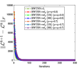
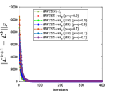
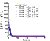
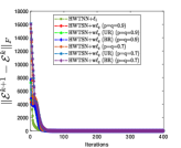
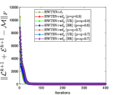
Firstly, we verify the accuracy/effectiveness of the proposed algorithm as well as the compared ones on the following two types of synthetic tensors: (I) $N_{1}=N_{2}=N,N\in\{1000,2000\},N_{3}=N_{4}=5$; (II) $N_{1}=N_{2}=N,N\in\{1000,2000\},N_{3}=N_{4}=N_{5}=3$. In our experiments, we set $R=0.05\cdot\min(N_{1},N_{2}),sr=0.5,\tau\in\{0.4,0.2\}$, $p,q\in\{0.9,0.7\}$, $\mathfrak{L}\in\{\text{FFT},\text{DCT},\text{ROT}\}$, $b=\lfloor\frac{k+5}{3}\rfloor,t=1$, $\vartheta=1.1,\beta^{0}=10^{-3},\beta^{\max}=10^{8},\varpi=10^{-6},\epsilon_{1}=\epsilon_{2}=10^{-16}$, $c_{1}=\alpha\cdot\min(N_{1},N_{2})$, $\alpha\in\{5,10,15,20,25\}$, $c_{2}=1$, and $\lambda\in\{0.02,0.03,0.05,0.08\}$. The experimental results are presented in Table II and Table III, from which we can observed that the RelError values obtained from the proposed method are relatively small in all case, which indicates that the proposed algorithm can accurately complete the latent low T-SVD rank tensor ${{\boldsymbol{\mathcal{L}}}}$ while removing the noise/outliers. Besides, the versions integrated with randomized techniques can greatly shorten the computational time under different linear transforms $\mathfrak{L}$. (I) $\mathfrak{L}=\small{\text{FFT}}$ (II) $\mathfrak{L}=\small{\text{DCT}}$ (III) $\mathfrak{L}=\small{\text{ROT}}$ Figure 2: The convergence behavior of the proposed and competitive RHTC algorithms. The x-coordinate is the number of iterations, the y-coordinates are the sequence Chg$1$-Chg$3$.

VI-A2 Convergence Study

Secondly, we mainly analyze the convergence behavior of the proposed and competitive algorithms on the following synthetic tensor: $N_{1}=N_{2}=1000,N_{3}=N_{4}=N_{5}=3,R=50,sr=0.5,\tau=0.4$. The parameter settings of the proposed algorithm are the same as those utilized in the previous experiments. Then, we record three type values, i.e., $\operatorname{Chg1}:={\|{\boldsymbol{\mathcal{L}}}^{k+1}-{\boldsymbol{\mathcal{L}}}^{k}\|{{}_{\mathnormal{F}}}}$, $\operatorname{Chg2}:={\|{\boldsymbol{\mathcal{E}}}^{k+1}-{\boldsymbol{\mathcal{E}}}^{k}\|{{}_{\mathnormal{F}}}}$, $\operatorname{Chg3}:={\|{\boldsymbol{\mathcal{M}}}-{\boldsymbol{\mathcal{L}}}^{k+1}-{\boldsymbol{\mathcal{E}}}^{k+1}\|{{}_{\mathnormal{F}}}}$, obtained by various RHTC algorithms at the $k$-th iteration, respectively. The recorded results are plotted in Figure 2, which is exactly consistent with the Theorem V.2, i.e., the obtained $\operatorname{Chg1}$, $\operatorname{Chg2}$, and $\operatorname{Chg3}$ gradually approach $0$ when the proposed algorithm iterates to a certain number of times.

VI-B Real-World Applications

Experiment Settings: In this subsection, we apply the proposed method (HWTSN+w$\ell_{q}$) and its two accelerated versions to several real-world applications, and also compare it with other RLRTC approaches: SNN+$\ell_{1}$[11], TRNN+$\ell_{1}$ [15], TTNN+$\ell_{1}$ [24], TSP-$k$+$\ell_{1}$ [23], LNOP [27], NRTRM [29], and HWTNN+$\ell_{1}$ [61]. In our experiments, we normalize the gray-scale value of the tested tensors to the interval $[0,1]$. For the RLRTC methods based on third-order T-SVD, we reshape the last two or three modes of tested tensors into one mode. The observed tensor is constructed as follows: the random-valued impulse noise with ratio $\tau$ is uniformly and randomly added to each frontal slice of the ground-truth tensor, and then we sample ($sr\cdot\prod_{i=1}^{d}n_{i}$) pixels from the noisy tensor to form the observed tensor $\boldsymbol{\bm{P}}_{{{\Omega}}}({\boldsymbol{\mathcal{M}}})$ at random. Unless otherwise stated, all parameters involved in the competing methods were optimally assigned or selected as suggested in the reference papers. The Peak Signal-to-Noise Ratio (PSNR), the structural similarity (SSIM), and the CPU time are employed to evaluate the recovery performance. Observed SNN+$\ell_{1}$ TRNN+$\ell_{1}$ TTNN+$\ell_{1}$ TSP-$k$+$\ell_{1}$ LNOP NRTRM HWTNN+$\ell_{1}$ HWTSN+w$\ell_{q}$ HWTSN+w$\ell_{q}$ (BR) HWTSN+w$\ell_{q}$ (UR) Ground truth Figure 3: Visual comparison of various methods for LFIs recovery. From top to bottom, the parameter pair $(sr,\tau)$ are $(0.05,0.5)$, $(0.1,0.5)$, $(0.05,0.3)$ and $(0.1,0.3)$, respectively. Top row: the $(6,6)$-th frame of Bench. The second row: the $(9,9)$-th frame of Bee-1. The third row: the $(12,12)$-th frame of Mini. Bottom row: the $(15,15)$-th frame of Framed. TABLE IV: The PSNR, SSIM values and CPU time obtained by various RLRTC methods for different fifth-order LFIs. The best and the second-best results are highlighted in blue and red, respectively.

LFI-Name Bench Bee-1 Framed Mini Average Time (s) $sr$ $5\%$ $10\%$ $5\%$ $10\%$ $5\%$ $10\%$ $5\%$ $10\%$ $\tau$ $30\%$ $50\%$ $30\%$ $50\%$ $30\%$ $50\%$ $30\%$ $50\%$ $30\%$ $50\%$ $30\%$ $50\%$ $30\%$ $50\%$ $30\%$ $50\%$ SNN+$\ell_{1}$ 14.29 0.176 11.94 0.091 14.81 0.267 13.69 0.168 12.72 0.137 11.07 0.081 13.39 0.179 11.74 0.128 12.76 0.203 11.47 0.112 13.99 0.269 11.67 0.179 14.29 0.195 12.92 0.132 15.99 0.245 15.37 0.197 10871 TRNN+$\ell_{1}$ 18.16 0.446 14.89 0.312 21.27 0.574 17.29 0.337 18.04 0.356 13.71 0.224 22.74 0.474 16.66 0.316 19.07 0.511 14.02 0.355 23.07 0.643 17.32 0.469 20.83 0.483 16.16 0.394 25.25 0.658 19.72 0.408 9111 TTNN+$\ell_{1}$ 21.65 0.704 16.48 0.434 23.04 0.746 20.72 0.608 22.44 0.776 16.24 0.353 24.74 0.831 20.75 0.464 23.33 0.797 16.95 0.516 25.37 0.857 22.13 0.667 25.67 0.775 17.51 0.486 27.45 0.818 22.92 0.638 4708 TSP-$k$+$\ell_{1}$ 22.33 0.687 17.43 0.415 24.02 0.785 21.21 0.611 22.88 0.734 17.08 0.333 25.62 0.843 21.32 0.456 23.43 0.772 17.81 0.491 25.67 0.863 22.24 0.661 26.36 0.757 18.04 0.489 29.02 0.857 23.93 0.663 6798 LNOP 21.87 0.628 18.35 0.436 27.02 0.813 21.84 0.649 22.46 0.658 18.08 0.348 28.37 0.879 21.87 0.512 22.88 0.674 19.05 0.493 28.83 0.839 22.79 0.637 24.58 0.658 20.97 0.529 30.89 0.853 25.73 0.725 6465 NRTRM 23.67 0.764 19.41 0.458 26.41 0.838 22.63 0.703 25.46 0.834 19.01 0.362 28.89 0.891 23.73 0.599 26.05 0.864 20.53 0.541 29.11 0.927 24.84 0.789 28.30 0.829 20.31 0.518 31.92 0.913 26.59 0.773 6267 HWTNN+$\ell_{1}$ 25.63 0.808 21.94 0.543 27.77 0.857 23.95 0.705 28.24 0.839 22.29 0.407 30.53 0.896 25.25 0.564 28.45 0.893 23.03 0.583 31.08 0.931 26.39 0.767 30.89 0.872 25.41 0.629 33.29 0.919 28.44 0.776 5754 HWTSN+w$\ell_{q}$ 26.85 0.834 23.44 0.671 30.13 0.892 26.29 0.808 29.56 0.889 25.28 0.651 33.03 0.938 27.69 0.723 29.95 0.916 25.55 0.743 33.78 0.961 29.89 0.915 32.25 0.902 28.99 0.766 35.82 0.952 32.78 0.898 7080 HWTSN+w$\ell_{q}$(BR) 24.83 0.743 22.86 0.645 25.36 0.746 24.62 0.721 28.16 0.846 24.85 0.661 28.69 0.874 27.79 0.847 28.15 0.863 25.25 0.735 29.01 0.884 27.98 0.868 29.39 0.808 27.29 0.723 29.55 0.817 29.19 0.811 2869 HWTSN+w$\ell_{q}$(UR) 24.92 0.741 22.96 0.649 25.46 0.749 24.78 0.728 28.74 0.846 24.94 0.663 28.76 0.874 27.88 0.848 28.23 0.864 25.28 0.736 29.19 0.886 28.29 0.869 29.46 0.809 27.38 0.725 29.67 0.816 29.25 0.812 2944

** In each RLRTC method, the top represents the PSNR values while the bottom denotes the SSIM values.

Parameters Setting: The transform in TTNN+$\ell_{1}$, NRTRM, HWTNN+$\ell_{1}$, and HWTSN+w$\ell_{q}$ is set as the FFT for consistency. The parameter $\lambda$ of SNN+$\ell_{1}$ is set as $\textbf{$\lambda$}\in\{[10,10,1,1]*\alpha,[10,10,1,1,1]*\alpha\}$, $\alpha\in\{1,3,5,8,10\}$. For TRNN+$\ell_{1}$, we set $\lambda\in\{0.018,0.015,0.012,0.01,0.009,0.007\}$. For TTNN+$\ell_{1}$, we set $\lambda=\varsigma/(\max{(n_{1},n_{2})}\cdot\prod_{i=3}^{d}n_{i})^{1/2}$, $\varsigma\in\{1,1.2,1.5,1.8,2\}$. For TSP-$k$+$\ell_{1}$, we set $k\in\{3,4,5\},\lambda\in\{100,200,300,400\}$. For LNOP, the parameter $p$ of $\ell_{p}$-ball projection is set to be $0.7$, $\epsilon=500,\lambda=10^{7}$. For NRTRM, the minimax concave penalty (MCP) function is utilized in both regularizers $G_{1},G_{2}$, the parameter $\eta$ of MCP is chosen as $\max(n_{1},n_{2})/\alpha^{k}$ for $G_{1}$ and $1/\beta^{k}$ for $G_{2}$, respectively; $c\in\{0.7,0.9,1.4\}$, and $\lambda={\kappa}/(\max{(n_{1},n_{2})}\cdot\prod_{i=3}^{d}n_{i})^{1/2}$, $\kappa\in\{1.2,1.5,1.8,2,2.2,2.5\}$. For HWTNN+$\ell_{1}$, we set $c=\max(n_{1},n_{2}),\epsilon=10^{-16}$ and $\lambda=\theta/(\max{(n_{1},n_{2})}\cdot\prod_{i=3}^{d}n_{i})^{1/2}$, $\theta\in\{25,30,35,40,45,50,55,60,65,70\}$. For our algorithms, we set $t=1,\vartheta=1.15,\beta^{0}=10^{-3},\beta^{\max}=10^{8},\varpi=10^{-4},\epsilon_{1}=\epsilon_{2}=10^{-16}$, $c_{1}=\omega\cdot\max(n_{1},n_{2})$, $\omega\in\{0.5,1,2,5,10,15,20,25,30\}$, $c_{2}=1$, $\lambda=\xi/(\max{(n_{1},n_{2})}\cdot\prod_{i=3}^{d}n_{i})^{1/2}$, $\xi\in\{1,3,5,6,8,10,12,15\}$, $k=100,b=20$ for multitemporal remote sensing images ($k=50,b=10$ for color videos and light field images). The adjustable parameters $p$ and $q$ are set to be inversely proportional to the constant $c_{1}$, respectively. In other words, as $p$ and $q$ go up, $\omega$ goes down.

VI-B1 Application in Light Field Images Recovery

In this experiment, we choose four fifth-order light field images (LFIs) including Bench, Bee-1, Framed and Mini to showcase the superiority and effectiveness of the proposed algorithms. These LFIs with the size of $434\times 625\times 3\times 15\times 15$ can be downloaded from the lytro illum light field dataset website . Observed SNN+$\ell_{1}$ TRNN+$\ell_{1}$ TTNN+$\ell_{1}$ TSP-$k$+$\ell_{1}$ LNOP NRTRM HWTNN+$\ell_{1}$ HWTSN+w$\ell_{q}$ HWTSN+w$\ell_{q}$ (BR) HWTSN+w$\ell_{q}$ (UR) Ground truth Figure 4: Visual comparison of various methods for CVs restoration. From top to bottom, the parameter pair $(sr,\tau)$ are $(0.1,0.3)$, $(0.1,0.5)$, $(0.2,0.3)$ and $(0.2,0.5)$, respectively. Top row: the $60$-th frame of Rush-hour. The second row: the $50$-th frame of Stockholm. The third row: the $34$-th frame of Intotree. Bottom row: the $10$-th frame of Johnny. TABLE V: The PSNR, SSIM values and CPU time obtained by various RLRTC methods for different fourth-order CVs. The best and the second-best results are highlighted in blue and red, respectively.

CV-Name Rush-hour Johnny Stockholm Intotree Average Time (s) $sr$ $10\%$ $20\%$ $10\%$ $20\%$ $10\%$ $20\%$ $10\%$ $20\%$ $\tau$ $30\%$ $50\%$ $30\%$ $50\%$ $30\%$ $50\%$ $30\%$ $50\%$ $30\%$ $50\%$ $30\%$ $50\%$ $30\%$ $50\%$ $30\%$ $50\%$ SNN+$\ell_{1}$ 18.37 0.711 17.26 0.559 21.78 0.771 19.57 0.689 18.03 0.758 16.61 0.734 21.80 0.803 18.61 0.745 19.96 0.501 18.96 0.484 21.42 0.537 20.53 0.502 20.81 0.591 18.88 0.512 23.08 0.622 21.85 0.539 12968 TRNN+$\ell_{1}$ 23.79 0.733 20.47 0.701 26.28 0.811 23.02 0.718 24.59 0.765 19.84 0.739 27.18 0.847 23.06 0.755 22.19 0.499 20.77 0.488 23.48 0.594 21.64 0.512 24.54 0.599 22.28 0.567 25.97 0.631 23.64 0.572 6968 TTNN+$\ell_{1}$ 24.77 0.758 22.39 0.734 28.13 0.833 24.94 0.753 27.29 0.868 24.19 0.782 30.57 0.911 26.93 0.791 23.02 0.609 21.32 0.494 25.82 0.649 22.82 0.567 25.51 0.605 23.64 0.577 27.54 0.632 24.99 0.602 5843 TSP-$k$+$\ell_{1}$ 26.59 0.819 23.46 0.741 28.68 0.845 25.46 0.808 29.42 0.886 24.98 0.813 31.55 0.912 27.48 0.835 24.39 0.643 21.81 0.526 26.08 0.686 23.24 0.593 26.58 0.633 23.64 0.578 27.85 0.637 24.85 0.617 9924 LNOP 26.67 0.830 23.31 0.748 29.13 0.857 25.91 0.829 28.03 0.768 23.69 0.742 29.55 0.861 28.39 0.832 24.66 0.638 22.39 0.533 26.85 0.694 24.43 0.603 26.24 0.609 23.78 0.603 27.70 0.634 25.95 0.623 9138 NRTRM 26.52 0.831 23.94 0.772 29.06 0.855 25.16 0.776 28.91 0.891 25.96 0.838 31.61 0.919 27.27 0.868 24.33 0.642 22.19 0.538 26.21 0.706 22.89 0.605 26.49 0.639 24.46 0.611 27.86 0.661 25.19 0.632 7834 HWTNN+$\ell_{1}$ 29.23 0.839 26.09 0.777 32.22 0.876 28.22 0.838 31.25 0.893 28.16 0.843 34.24 0.923 30.43 0.876 26.16 0.663 23.34 0.551 28.38 0.718 24.66 0.627 27.49 0.647 25.56 0.619 28.72 0.687 26.27 0.643 6737 HWTSN+w$\ell_{q}$ 30.27 0.851 27.38 0.794 33.68 0.885 30.02 0.867 32.36 0.905 29.45 0.868 35.33 0.931 32.07 0.907 26.86 0.668 24.01 0.554 28.62 0.741 26.89 0.707 27.92 0.659 26.53 0.638 28.98 0.695 27.94 0.667 8760 HWTSN+w$\ell_{q}$(BR) 29.15 0.841 26.66 0.784 31.27 0.868 28.89 0.850 29.85 0.868 28.06 0.844 30.66 0.879 29.46 0.869 26.50 0.686 24.19 0.579 29.21 0.755 26.19 0.688 27.60 0.649 26.16 0.623 28.43 0.679 27.38 0.658 4243 HWTSN+w$\ell_{q}$(UR) 29.28 0.842 26.77 0.789 31.41 0.865 29.03 0.852 29.93 0.869 28.19 0.844 30.76 0.878 29.53 0.870 26.60 0.688 24.27 0.582 29.27 0.758 26.30 0.692 27.68 0.651 26.21 0.625 28.45 0.684 27.48 0.659 4374

** In each RLRTC method, the top represents the PSNR values while the bottom denotes the SSIM values.

Figure 3 shows the recovered LFIs and corresponding zoomed regions acquired by different RLRTC methods at extremely low sampling rates. From the enlarged areas, we can observed that the LFIs restored by our method preserves more details than those achieved by other competitive algorithms. The PSNR, SSIM values and average CPU time of various RLRTC methods for four LFIs with different noise levels and observation ratios are displayed in Table IV. The following conclusions can be drawn from above quantitative metrics. 1) Classical methods induced by the Tucker and TR format, i.e., SNN+$\ell_{1}$ and TRNN+$\ell_{1}$, perform relative poorer in term of recovery quality. 2) Among those algorithms induced by third-order T-SVD, although the ones employing nonconvex schemes (i.e., LNOP and NRTRM) require more running time over the ones utilizing convex methods (i.e., TTNN+$\ell_{1}$ and TSP-$k$+$\ell_{1}$), they achieve higher PSNR and SSIM values in most cases. This phenomenon also exists in the methods based on high-order T-SVD. 3) Compared with other methods, the HWTSN+w$\ell_{q}$ achieves an approximately $2$$\sim$$5$ dB gain in the mean PSNR values, and its accelerated versions obtains an about $40\%$$\sim$$60\%$ percent drop in the average CPU time. 4) In our algorithms, the versions fused randomization ideas shorten the running time by about $55\%$ percent over the deterministic version with a slight reduction of psnr and ssim values.

VI-B2 Application in Color Videos Restoration

In this experiment, color videos (CVs) are used to evaluate the performance of the proposed algorithm. We download four large-scale CVs from the derf website for this test. Only the first $100$ frames of each video sequence are selected as the test data owing to the computational limitation, in which each frame has the size $720\times 1280\times 3$. For each CV with $100$ frames, it can be formulated as an $720\times 1280\times 3\times 100$ fourth-order tensor. Figure 4 displays the visual comparison of the proposed and competitive RLRTC algorithms for various CVs restoration. From the zoomed regions, we can see that the HWTSN+w$\ell_{q}$ exhibits tangibly better restortation quality over other comparative methods according to the color, brightness, and outline. In Table V, we report the PSNR, SSIM values and CPU time of ten RLRTC methods for four CVs, where $sr=0.1,0.2$ and $\tau=0.3,0.5$. These results show that the PSNR and SSIM metrics acquired by HWTSN+w$\ell_{q}$ are higher than those obtained by the baseline method, i.e., HWTNN+$\ell_{1}$. In contrast to the competitive non-convex methods (i.e., LNOP and NRTRM), the improvements of proposed non-convex algorithm (i.e.,HWTSN+w$\ell_{q}$) are around $3$ dB in term of PSNR index while the reductions of its randomized version are about $52\%$ according to the CPU time. Furthermore, under the comprehensive balance of PSNR, SSIM, and CPU time, the proposed randomized RHTC method is always superior to other popular algorithms. Other findings are similar to the case of LFIs recovery.

VI-B3 Application in Multitemporal Remote Sensing Images Inpainting

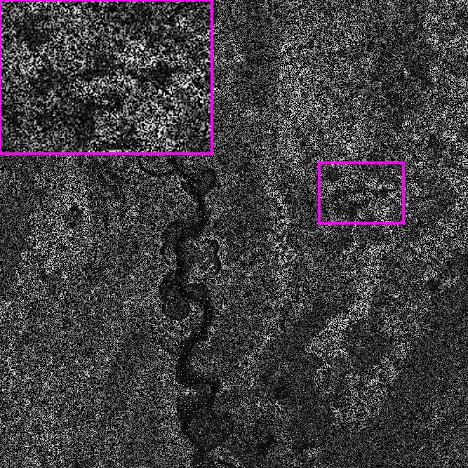
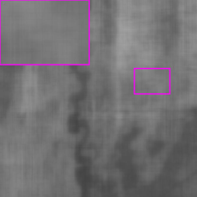
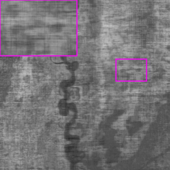
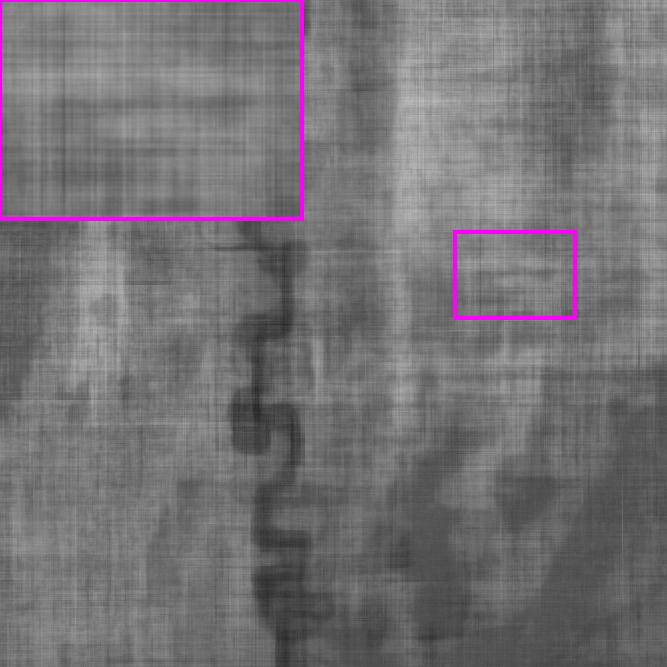
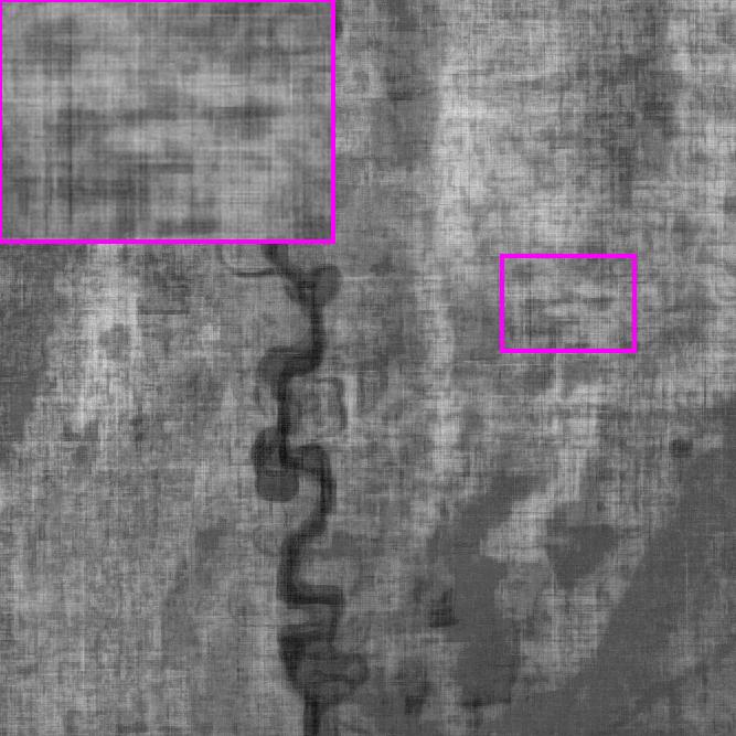
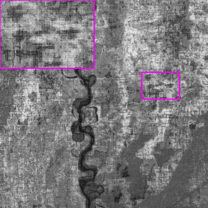
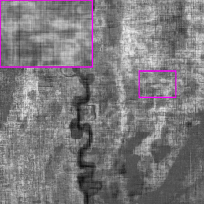
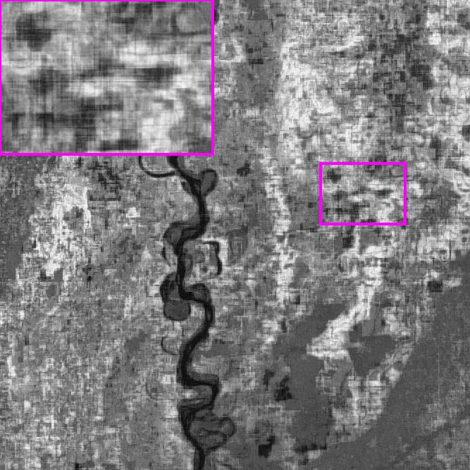
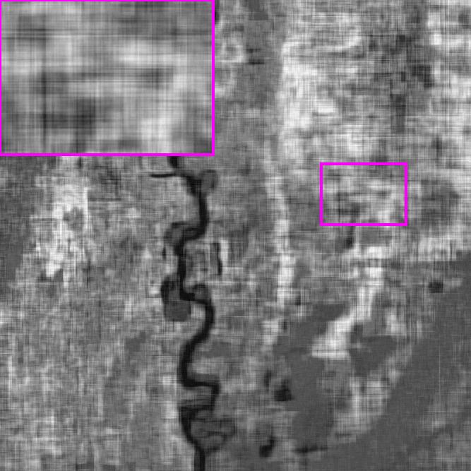
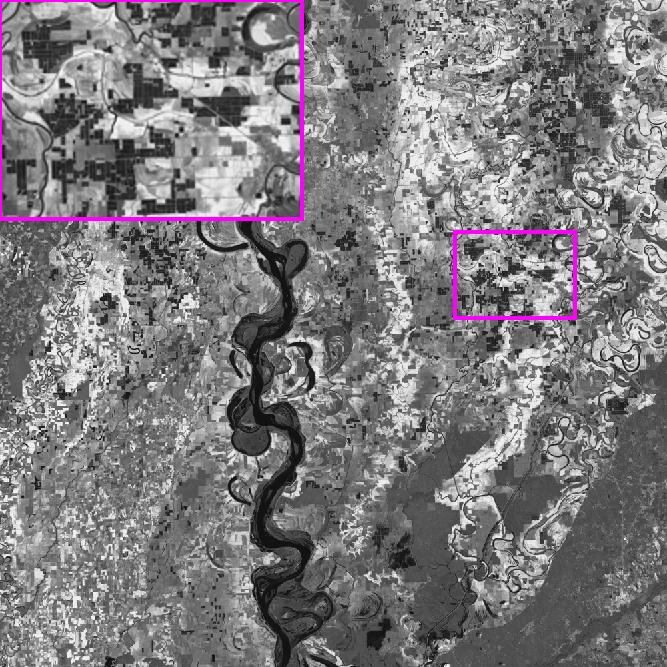
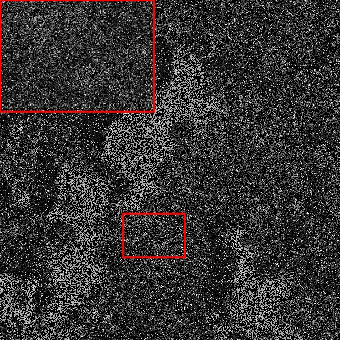
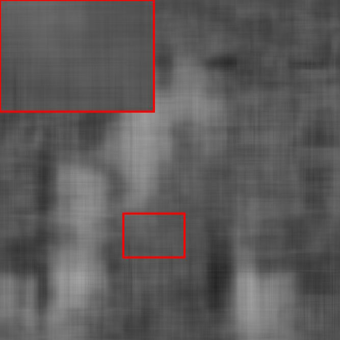
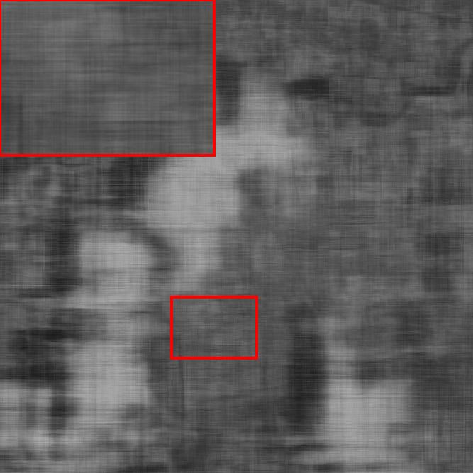
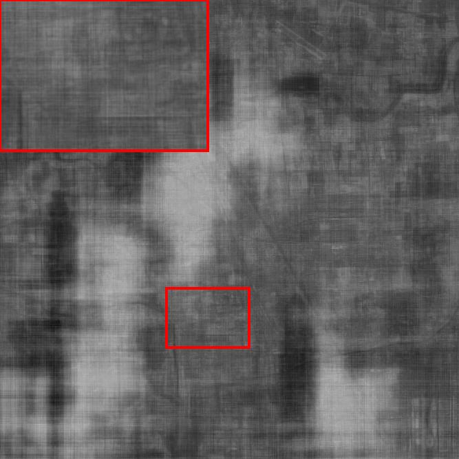
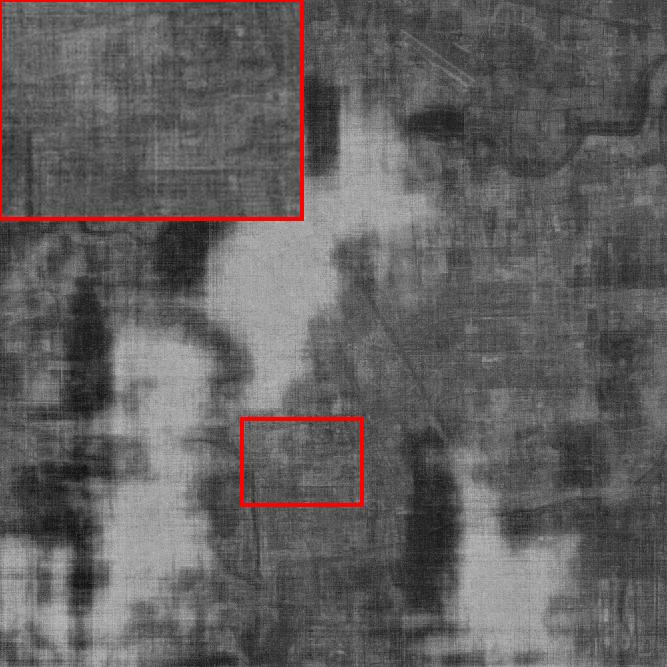
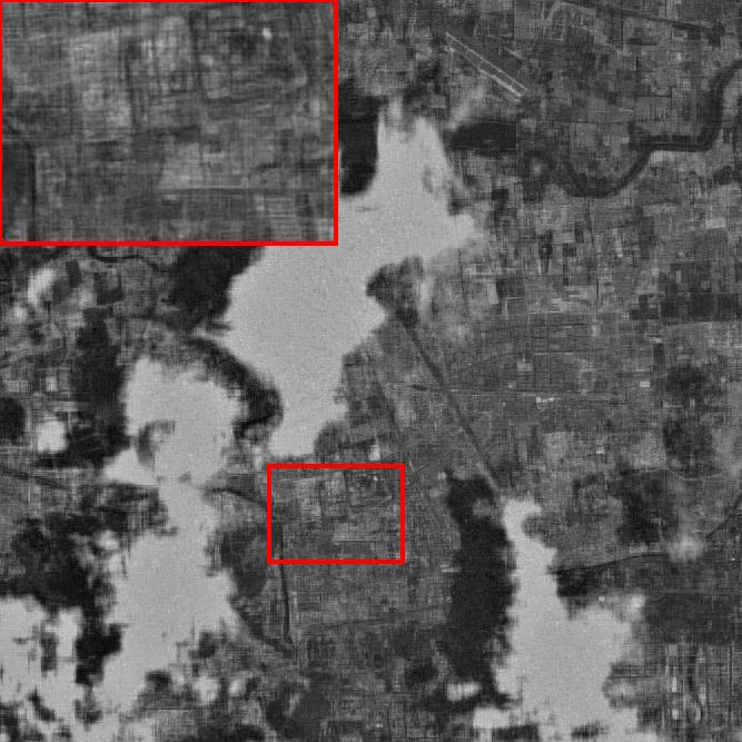
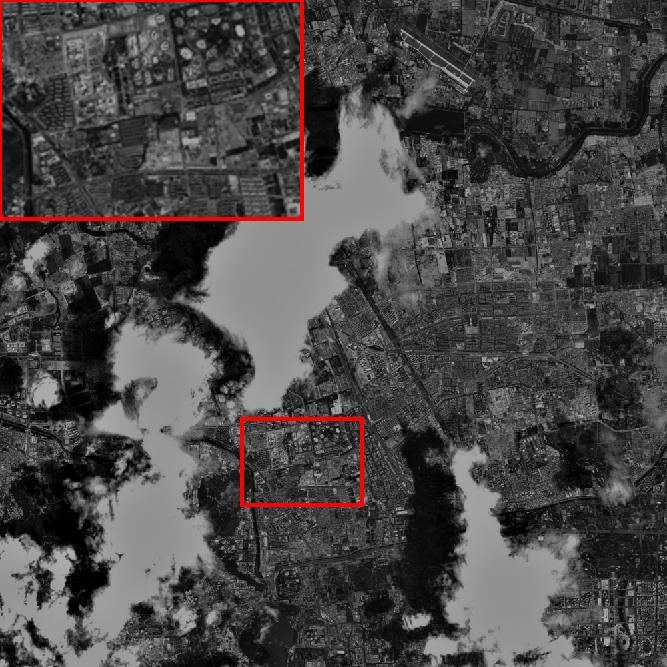
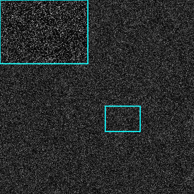
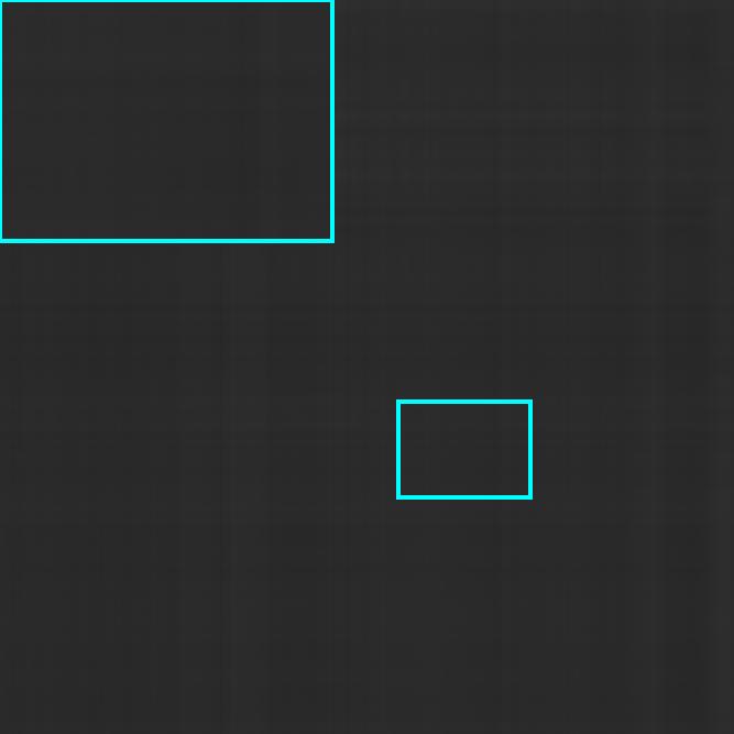
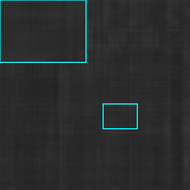
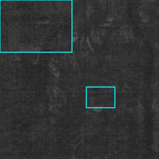
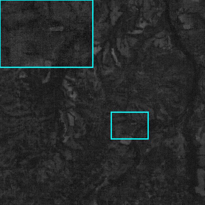
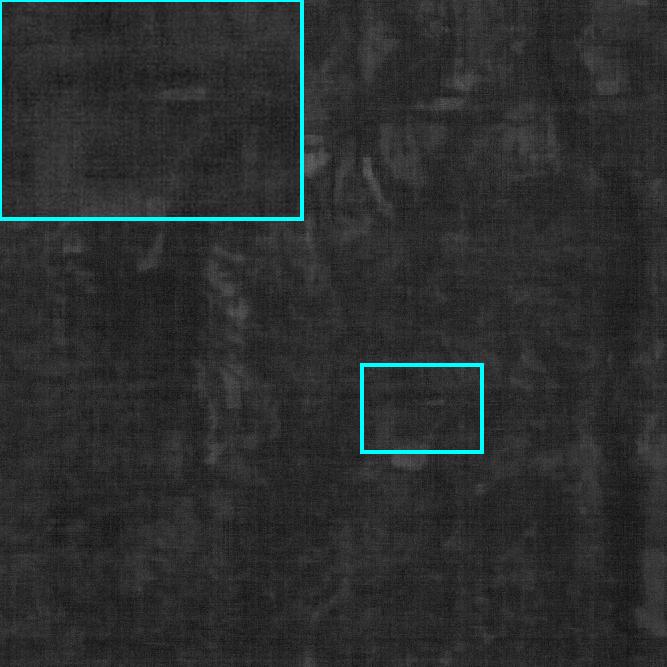
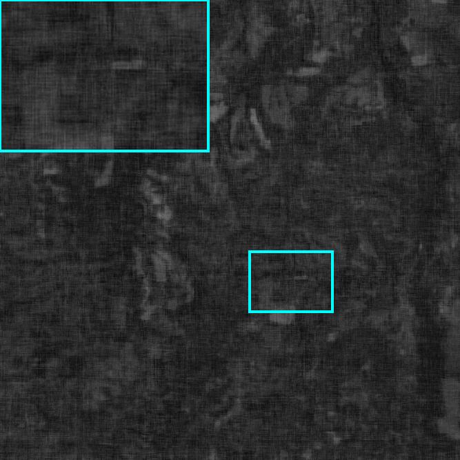
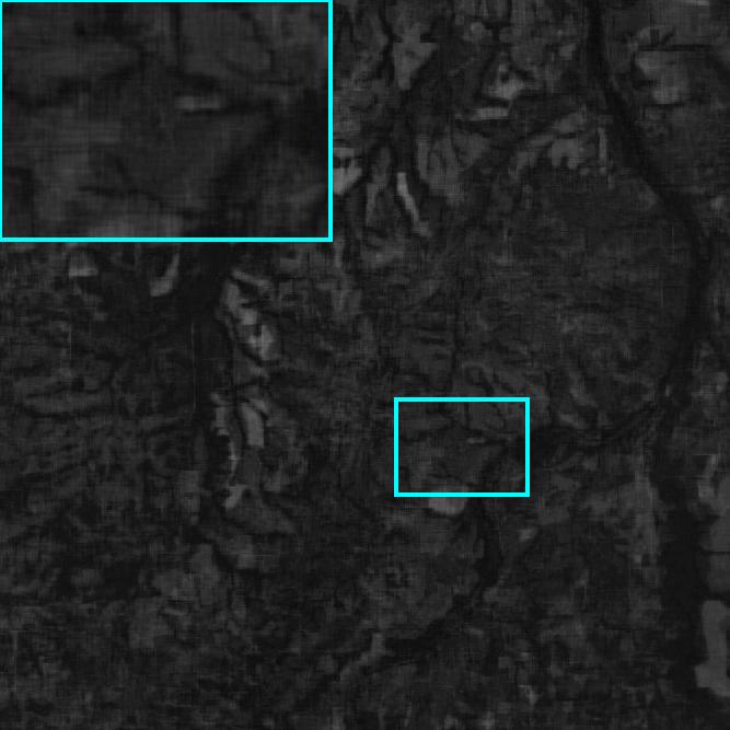
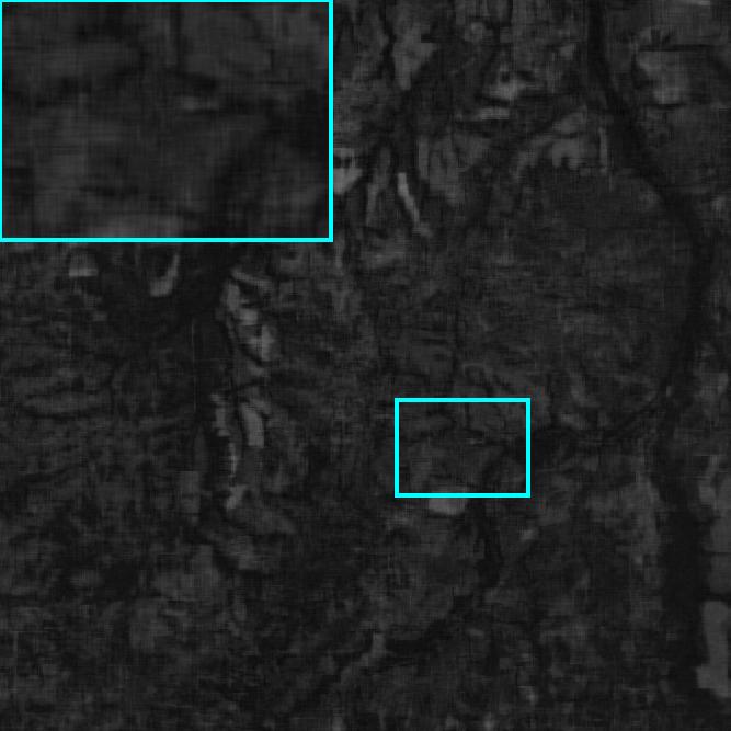
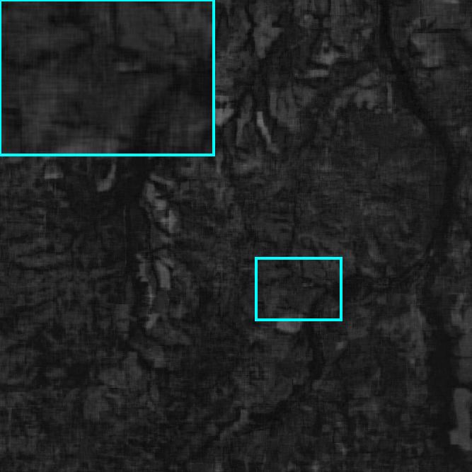
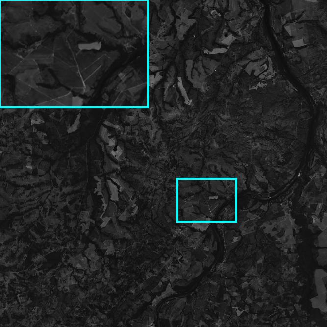
This experiment mainly tests three fourth-order multi-temporal remote sensing images (MRSIs), which are named SPOT-5 ($2000\times 2000\times 4\times 13$), Landsat-7 ($4500\times 4500\times 6\times 11$), and T22LGN ($5001\times 5001\times 4\times 7$), respectively. To speed up the calculation process, the spatial size of these MRSIs is downsampled (resized) to $2000\times 2000$. Observed SNN+$\ell_{1}$ TRNN+$\ell_{1}$ TTNN+$\ell_{1}$ TSP-$k$+$\ell_{1}$ LNOP NRTRM HWTNN+$\ell_{1}$ HWTSN+w$\ell_{q}$ HWTSN+w$\ell_{q}$ (BR) HWTSN+w$\ell_{q}$ (UR) Ground truth Figure 5: Visual comparison of various methods for MRSIs inpainting. From top to bottom, the parameter pair $(sr,\tau)$ are $(0.4,0.1)$, $(0.4,0.3)$, and $(0.4,0.5)$, respectively. Top row: the $(5,1)$-th frame of Landsat-7. Middle row: the $(2,6)$-th frame of SPOT-5. Bottom row: the $(3,5)$-th frame of T22LGN. TABLE VI: The PSNR, SSIM values and CPU time obtained by various RLRTC methods for different fourth-order MRSIs. The best and the second-best results are highlighted in blue and red, respectively.

MRSI-Name Landsat-7 T22LGN SPOT-5 Average Time (s) $sr$ $20\%$ $40\%$ $20\%$ $40\%$ $20\%$ $40\%$ $\tau$ $10\%$ $30\%$ $50\%$ $10\%$ $30\%$ $50\%$ $10\%$ $30\%$ $50\%$ $10\%$ $30\%$ $50\%$ $10\%$ $30\%$ $50\%$ $10\%$ $30\%$ $50\%$ SNN+$\ell_{1}$ 21.45 0.537 20.86 0.453 20.13 0.386 23.12 0.576 22.49 0.498 21.44 0.477 25.94 0.637 25.91 0.605 25.69 0.592 27.01 0.718 26.68 0.666 25.76 0.596 22.38 0.573 21.58 0.509 20.91 0.395 25.63 0.631 24.19 0.563 22.55 0.492 23817 TRNN+$\ell_{1}$ 23.96 0.671 22.32 0.589 20.70 0.565 24.61 0.699 22.67 0.691 21.30 0.614 28.57 0.716 27.22 0.696 25.02 0.586 29.15 0.797 27.52 0.723 25.89 0.666 27.06 0.681 24.55 0.568 22.16 0.467 28.19 0.716 25.07 0.584 23.11 0.523 22414 TTNN+$\ell_{1}$ 23.17 0.652 21.89 0.543 20.19 0.458 24.05 0.739 22.61 0.691 21.15 0.575 29.88 0.793 28.34 0.778 24.58 0.497 31.26 0.817 29.37 0.797 26.29 0.692 26.49 0.684 24.38 0.537 22.22 0.431 28.17 0.701 25.65 0.596 23.49 0.519 10107 TSP-$k$+$\ell_{1}$ 24.07 0.673 22.41 0.588 20.36 0.461 25.82 0.742 23.62 0.628 21.14 0.472 29.12 0.791 25.22 0.511 22.54 0.409 31.14 0.836 26.03 0.545 22.59 0.419 27.07 0.657 24.57 0.571 22.29 0.413 29.74 0.775 26.36 0.601 23.34 0.506 27412 LNOP 24.61 0.679 22.72 0.658 20.83 0.589 26.27 0.763 23.35 0.688 21.42 0.592 30.98 0.841 28.61 0.736 26.43 0.703 33.63 0.919 29.12 0.825 26.89 0.706 27.66 0.643 25.55 0.593 23.45 0.484 29.88 0.781 26.63 0.632 24.66 0.572 18418 NRTRM 23.76 0.669 22.40 0.626 20.45 0.546 25.72 0.757 23.84 0.639 21.33 0.577 30.34 0.833 28.67 0.782 25.68 0.607 33.12 0.893 30.41 0.844 25.87 0.621 27.08 0.682 24.84 0.589 22.55 0.432 29.95 0.799 26.84 0.645 23.73 0.569 18560 HWTNN+$\ell_{1}$ 25.18 0.692 23.48 0.659 21.59 0.630 26.33 0.768 24.98 0.693 22.89 0.665 32.09 0.854 29.19 0.758 25.53 0.639 34.24 0.923 31.46 0.852 26.46 0.706 28.45 0.687 26.24 0.596 23.61 0.490 30.47 0.808 28.36 0.699 25.49 0.581 14835 HWTSN+w$\ell_{q}$ 25.99 0.722 24.71 0.683 23.21 0.669 28.11 0.777 25.99 0.724 23.61 0.677 32.46 0.888 30.16 0.833 27.98 0.746 34.98 0.944 31.92 0.896 28.64 0.794 29.58 0.713 27.79 0.615 25.82 0.565 32.47 0.836 30.07 0.756 26.77 0.644 18974 HWTSN+w$\ell_{q}$(BR) 24.94 0.682 24.30 0.662 22.88 0.641 25.55 0.729 24.94 0.711 23.13 0.674 30.54 0.809 29.32 0.791 27.79 0.738 30.94 0.819 30.02 0.814 28.39 0.777 27.94 0.624 27.19 0.599 25.48 0.551 28.72 0.695 28.19 0.675 26.37 0.614 5412 HWTSN+w$\ell_{q}$(UR) 25.02 0.683 24.37 0.676 22.91 0.645 25.69 0.729 25.05 0.712 23.15 0.674 30.65 0.811 29.39 0.792 27.81 0.739 31.06 0.822 30.17 0.816 28.45 0.779 27.99 0.624 27.21 0.605 25.51 0.557 28.82 0.694 28.26 0.686 26.40 0.617 5746

** In each RLRTC method, the top represents the PSNR values while the bottom denotes the SSIM values.

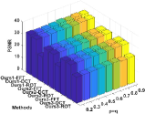
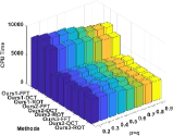
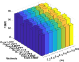
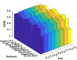
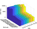
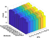
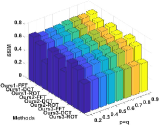
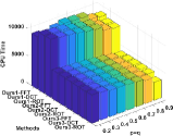
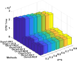
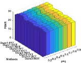
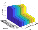
Table VI presents the PSNR, SSIM values and CPU time provided by ten RLRTC methods on three large-scale MRSIs with $sr\in\{0.4,0.2\}$, $\tau\in\{0.1,0.3,0.5\}$. Accordingly, some visual examples are illustrated in Figure 5, which indicates that the proposed method retains more details and textures over the other state-of-the-art approaches. Strikingly, in comparison with the deterministic RLRTC algorithms, our RHTC algorithms incorporating with randomized technology can decrease the computational time by about $70\%$ with little or no loss of PSNR and SSIM. This demonstrates the effectiveness of randomized approach for processing large-scale tensor data. Other conclusions achieved from the quantitative results are similar to those obtained from the tasks of CVs restoration and LFIs recovery. Overall, the proposed randomized RHTC method can dramatically shorten the CPU running time while still achieving reasonable recovery precision over other popular approaches, especially for large-scale inpainting tasks. Figure 6: The influence of adjustable parameters $(p,q)$, and changing linear transforms $\mathfrak{L}$ upon LFIs recovery. Top row: $sr=0.1,\tau=0.3$, Bottom row: $sr=0.1,\tau=0.5$. Figure 7: The influence of adjustable parameters $(p,q)$, and changing linear transforms $\mathfrak{L}$ upon CVs restoration. Top row: $sr=0.2,\tau=0.3$, Bottom row: $sr=0.2,\tau=0.5$. Figure 8: The influence of adjustable parameters $(p,q)$, and changing linear transforms $\mathfrak{L}$ upon MRSIs inpainting. Top row: $sr=0.4,\tau=0.1$, Bottom row: $sr=0.4,\tau=0.3$.

VI-B4 Discussion

In the previous real applications, the proposed methods only employ the linear transform: FFT, and only set the adjustable parameters $(p,q)$ to be $(0.9,0.9)$. In this subsection, we additionally utilize other linear transforms (e.g., DCT, ROT) and adjustable parameters $(p,q)$ to perform related experiments on the proposed algorithm and its two accelerated versions. Our goal is to investigate the influence of adjustable parameters $(p,q)$, and changing invertible linear transforms $\mathfrak{L}$ upon restoration results of various tensor data with different noise levels and observed ratios in both deterministic and randomized approximation patterns. In our experiments, the values $p,q(p=q)$ are set from $0.2$ to $0.9$ with an interval of $0.1$. For brevity, the proposed algorithm: “HWTSN+w$\ell_{q}$”, and its accelerated versions: “HWTSN+w$\ell_{q}$(UR)” and “HWTSN+w$\ell_{q}$(BR)” are abbreviated as Ours1, Ours2, and Ours3, respectively. The corresponding experimental results of the above investigation are shown in Figure 6,7,8, from which some instructive conclusions and guidelines can be drawn. (I) The PSNR or SSIM value obtained by ROT is always worse than that achieved by FFT and DCT under the same parameters $p$ and $q$. This implies that ROT may not be a good choice for the restoration of real-world high-order tensors. (II) For the recovery of three types of tensors, with the increase of adjustable parameters $p$ and $q$, the PSNR and SSIM values obtained by various methods gradually increase whereas the corresponding running time gradually decreases in most cases. This suggests that selecting relatively large $p$ and $q$ may yield better recovery performance for different types of high-order tensors. (III) Just as we expected, in comparison with the deterministic version (i.e., Ours1), the randomized methods (i.e., Ours2 and Ours3) greatly boost the computational efficiency at the premise of compromising a little PSNR and SSIM for various inpainting tasks. (IV) In our randomized versions, there is remarkably little difference between Ours2 and Ours3 in CPU running time for different recovery tasks. This indicates that it is very likely that only for very large-scale tensors, the computational cost of Ours3 (i.e., the version fusing blocked randomized scheme) is significantly lower than that of Ours2.

VII Conclusions and Future Work

In this article, we first develop two efficient low-rank tensor approximation methods fusing random projection schemes, based on which we further study the effective model and algorithm for RHTC. The model construction, algorithm design and theoretical analysis are all based on the algebraic framework of high-order T-SVD. Extensive experiments on both synthetic and real-world tensor data have verified the effectiveness and superiority of the proposed approximation and completion approaches. This work will lay the foundation for many tensor-based data analysis tasks such as high-order tensor clustering, regression, classification, etc. In the future, under the T-SVD framework, we first intend to explore the effective randomized algorithm for the fixed-precision low-rank tensor approximation by devising novel mode-wise projection strategy that differs from the literature [79]. On this basis, we further investigate the high-order tensor recovery from the perspective of model, algorithm and theory. Secondly, we will exploit the fast high-order tensor clustering, regression and classification approaches in virtue of some popular randomized sketching techniques (e.g., random projection/sampling and count-sketch). Finally, we plan to extend the above batch-based randomized methods to the online versions, which can deal with large-scale streaming tensors incrementally in online mode, and even with dynamically changing tensors.

- [1] C. F. Beckmann and S. M. Smith, “Tensorial extensions of independent component analysis for multisubject fmri analysis,” Neuroimage, vol. 25, no. 1, pp. 294–311, 2005.
- [2] K. T. Schütt, F. Arbabzadah, S. Chmiela, K. R. Müller, and A. Tkatchenko, “Quantum-chemical insights from deep tensor neural networks,” Nat. Commun., vol. 8, no. 1, p. 13890, 2017.
- [3] E. E. Papalexakis, C. Faloutsos et al., “Tensors for data mining and data fusion: Models, applications, and scalable algorithms,” ACM Trans. Intell. Syst. Technol., vol. 8, no. 2, pp. 1–44, 2016.
- [4] N. D. Sidiropoulos, L. De Lathauwer, X. Fu, K. Huang et al., “Tensor decomposition for signal processing and machine learning,” IEEE Trans. Signal Process., vol. 65, no. 13, pp. 3551–3582, 2017.
- [5] M. Marquez, H. Rueda-Chacon, and H. Arguello, “Compressive spectral light field image reconstruction via online tensor representation,” IEEE Trans. Image Process., vol. 29, pp. 3558–3568, 2020.
- [6] J. Lin, T.-Z. Huang, X.-L. Zhao et al., “Robust thick cloud removal for multitemporal remote sensing images using coupled tensor factorization,” IEEE Trans. Geosci. Remote. Sens., vol. 60, pp. 1–16, 2022.
- [7] Z. Long, C. Zhu, J. Liu et al., “Bayesian low rank tensor ring for image recovery,” IEEE Trans. Image Process., vol. 30, pp. 3568–3580, 2021.
- [8] A. Bibi and B. Ghanem, “High order tensor formulation for convolutional sparse coding,” in Proc. IEEE Int. Conf. Comput. Vis. (ICCV), 2017, pp. 1772–1780.
- [9] X. Zhang, D. Wang, Z. Zhou, and Y. Ma, “Robust low-rank tensor recovery with rectification and alignment,” IEEE Trans. Pattern Anal. Mach. Intell., vol. 43, no. 1, pp. 238–255, 2019.
- [10] J. Hou, F. Zhang, H. Qiu, J. Wang, Y. Wang, and D. Meng, “Robust low-tubal-rank tensor recovery from binary measurements,” IEEE Trans. Pattern Anal. Mach. Intell., vol. 44, no. 8, pp. 4355–4373, 2021.
- [11] D. Goldfarb and Z. Qin, “Robust low-rank tensor recovery: Models and algorithms,” SIAM J. Matrix Anal. Appl., vol. 35, no. 1, pp. 225–253, 2014.
- [12] B. Huang, C. Mu et al., “Provable models for robust low-rank tensor completion,” Pac. J. Optim., vol. 11, no. 2, pp. 339–364, 2015.
- [13] Q. Zhao, G. Zhou, L. Zhang, A. Cichocki, and S.-I. Amari, “Bayesian robust tensor factorization for incomplete multiway data,” IEEE Trans. Neural Netw. Learn. Syst., vol. 27, no. 4, pp. 736–748, 2015.
- [14] W. Chen, X. Gong, and N. Song, “Nonconvex robust low-rank tensor reconstruction via an empirical bayes method,” IEEE Trans. Signal Process., vol. 67, no. 22, pp. 5785–5797, 2019.
- [15] H. Huang, Y. Liu, Z. Long, and C. Zhu, “Robust low-rank tensor ring completion,” IEEE Trans. Comput. Imag., vol. 6, pp. 1117–1126, 2020.
- [16] C. Chen, Z.-B. Wu et al., “Auto-weighted robust low-rank tensor completion via tensor-train,” Inf. Sci., vol. 567, pp. 100–115, 2021.
- [17] Q. Liu, X. Li, H. Cao, and Y. Wu, “From simulated to visual data: A robust low-rank tensor completion approach using -regression for outlier resistance,” IEEE Trans. Circuits Syst. Video Technol., vol. 32, no. 6, pp. 3462–3474, 2021.
- [18] X. P. Li and H. C. So, “Robust low-rank tensor completion based on tensor ring rank via -norm,” IEEE Trans. Signal Process., vol. 69, pp. 3685–3698, 2021.
- [19] Y. He and G. K. Atia, “Coarse to fine two-stage approach to robust tensor completion of visual data,” IEEE Trans. Cybern., 2022, doi: 10.1109/10.1109/TCYB.2022.3198932.
- [20] Q. Jiang and M. Ng, “Robust low-tubal-rank tensor completion via convex optimization.” in Proc. 28th Int. Joint Conf. Artif. Intell., 2019, pp. 2649–2655.
- [21] A. Wang, Z. Jin, and G. Tang, “Robust tensor decomposition via t-svd: Near-optimal statistical guarantee and scalable algorithms,” Signal Process., vol. 167, p. 107319, 2020.
- [22] A. Wang, X. Song, X. Wu, Z. Lai, and Z. Jin, “Robust low-tubal-rank tensor completion,” in Proc. IEEE Int. Conf. Acoust., Speech Signal Process. (ICASSP), 2019, pp. 3432–3436.
- [23] J. Lou and Y.-M. Cheung, “Robust low-rank tensor minimization via a new tensor spectral -support norm,” IEEE Trans. Image Process., vol. 29, pp. 2314–2327, 2019.
- [24] G. Song, M. K. Ng, and X. Zhang, “Robust tensor completion using transformed tensor singular value decomposition,” Numer. Linear Algebr. Appl., vol. 27, no. 3, p. e2299, 2020.
- [25] M. K. Ng, X. Zhang et al., “Patched-tube unitary transform for robust tensor completion,” Pattern Recognit., vol. 100, p. 107181, 2020.
- [26] Y. He and G. K. Atia, “Robust low-tubal-rank tensor completion based on tensor factorization and maximum correntopy criterion,” arXiv preprint arXiv:2010.11740, 2020.
- [27] L. Chen, X. Jiang, X. Liu, and Z. Zhou, “Robust low-rank tensor recovery via nonconvex singular value minimization,” IEEE Trans. Image Process., vol. 29, pp. 9044–9059, 2020.
- [28] X. Zhao, M. Bai, and M. K. Ng, “Nonconvex optimization for robust tensor completion from grossly sparse observations,” J. Sci. Comput., vol. 85, no. 2, pp. 1–32, 2020.
- [29] D. Qiu, M. Bai et al., “Nonlocal robust tensor recovery with nonconvex regularization,” Inverse Probl., vol. 37, no. 3, p. 035001, 2021.
- [30] X. Zhao, M. Bai, D. Sun, and L. Zheng, “Robust tensor completion: Equivalent surrogates, error bounds, and algorithms,” SIAM J. Imaging Sci., vol. 15, no. 2, pp. 625–669, 2022.
- [31] C. Lu, J. Feng, Y. Chen, W. Liu, Z. Lin, and S. Yan, “Tensor robust principal component analysis with a new tensor nuclear norm,” IEEE Trans. Pattern Anal. Mach. Intell., vol. 42, no. 4, pp. 925–938, 2019.
- [32] F. Zhang, J. Wang, W. Wang, and C. Xu, “Low-tubal-rank plus sparse tensor recovery with prior subspace information,” IEEE Trans. Pattern Anal. Mach. Intell., vol. 43, no. 10, pp. 3492–3507, 2021.
- [33] Q. Gao, P. Zhang, W. Xia, D. Xie, X. Gao, and D. Tao, “Enhanced tensor rpca and its application,” IEEE Trans. Pattern Anal. Mach. Intell., vol. 43, no. 6, pp. 2133–2140, 2020.
- [34] M. Li, W. Li, Y. Chen, and M. Xiao, “The nonconvex tensor robust principal component analysis approximation model via the weighted -norm regularization,” J. Sci. Comput., vol. 89, no. 3, pp. 1–37, 2021.
- [35] H. Qiu, Y. Wang, S. Tang et al., “Fast and provable nonconvex tensor rpca,” in Proc. Int. Conf. Mach. Learn. (ICML), 2022, pp. 18 211–18 249.
- [36] J. Wang, J. Hou, and Y. C. Eldar, “Tensor robust principal component analysis from multilevel quantized observations,” IEEE Trans. Inf. Theory, vol. 69, no. 1, pp. 383–406, 2022.
- [37] Y.-B. Zheng, T.-Z. Huang, X.-L. Zhao, T.-X. Jiang, T.-Y. Ji, and T.-H. Ma, “Tensor n-tubal rank and its convex relaxation for low-rank tensor recovery,” Inf. Sci., vol. 532, pp. 170–189, 2020.
- [38] Q. Shi, Y.-M. Cheung, and J. Lou, “Robust tensor svd and recovery with rank estimation,” IEEE Trans. Cybern., vol. 52, no. 10, pp. 10 667–10 682, 2021.
- [39] M. Yang, Q. Luo, W. Li, and M. Xiao, “Nonconvex 3d array image data recovery and pattern recognition under tensor framework,” Pattern Recognit., vol. 122, p. 108311, 2022.
- [40] Z. Zhang and S. Aeron, “Exact tensor completion using t-SVD,” IEEE Trans. Signal Process., vol. 65, no. 6, pp. 1511–1526, 2015.
- [41] H. Kong, X. Xie, and Z. Lin, “t-schatten- norm for low-rank tensor recovery,” IEEE J. Sel. Topics Signal Process., vol. 12, no. 6, pp. 1405–1419, 2018.
- [42] X. Zhang and M. K. Ng, “Low rank tensor completion with poisson observations,” IEEE Trans. Pattern Anal. Mach. Intell., vol. 44, no. 8, pp. 4239–4251, 2021.
- [43] H. Xu, J. Zheng, X. Yao, Y. Feng, and S. Chen, “Fast tensor nuclear norm for structured low-rank visual inpainting,” IEEE Trans. Circuits Syst. Video Technol., vol. 32, no. 2, pp. 538–552, 2021.
- [44] H. Wang, F. Zhang, J. Wang, T. Huang et al., “Generalized nonconvex approach for low-tubal-rank tensor recovery,” IEEE Trans. Neural Netw. Learn. Syst., vol. 33, no. 8, pp. 3305–3319, 2021.
- [45] J. Liu, P. Musialski, P. Wonka, and J. Ye, “Tensor completion for estimating missing values in visual data,” IEEE Trans. Pattern Anal. Mach. Intell., vol. 35, no. 1, pp. 208–220, 2013.
- [46] J. A. Bengua, H. N. Phien, H. D. Tuan, and M. N. Do, “Efficient tensor completion for color image and video recovery: Low-rank tensor train,” IEEE Trans. Image Process., vol. 26, no. 5, pp. 2466–2479, 2017.
- [47] X.-L. Zhao, J.-H. Yang, T.-H. Ma, T.-X. Jiang et al., “Tensor completion via complementary global, local, and nonlocal priors,” IEEE Trans. Image Process., vol. 31, pp. 984–999, 2021.
- [48] J. Xue, Y. Zhao, Y. Bu et al., “When laplacian scale mixture meets three-layer transform: A parametric tensor sparsity for tensor completion,” IEEE Trans. Cybern., vol. 52, no. 12, pp. 13 887–13 901, 2022.
- [49] Y. Qiu, G. Zhou, Q. Zhao, and S. Xie, “Noisy tensor completion via low-rank tensor ring,” IEEE Trans. Neural Netw. Learn. Syst., 2022, doi: 10.1109/TNNLS.2022.3181378.
- [50] T. G. Kolda and B. W. Bader, “Tensor decompositions and applications,” SIAM Rev., vol. 51, no. 3, pp. 455–500, 2009.
- [51] L. R. Tucker, “Some mathematical notes on three-mode factor analysis,” Psychometrika, vol. 31, no. 3, pp. 279–311, 1966.
- [52] I. V. Oseledets, “Tensor-train decomposition,” SIAM J. Sci. Comput., vol. 33, no. 5, pp. 2295–2317, 2011.
- [53] Q. Zhao, G. Zhou, S. Xie, L. Zhang, and A. Cichocki, “Tensor ring decomposition,” arXiv preprint arXiv:1606.05535, 2016.
- [54] M. E. Kilmer and C. D. Martin, “Factorization strategies for third-order tensors,” Linear Alg. Appl., vol. 435, no. 3, pp. 641–658, 2011.
- [55] E. Kernfeld, M. Kilmer et al., “Tensor–tensor products with invertible linear transforms,” Linear Alg. Appl., vol. 485, pp. 545–570, 2015.
- [56] M. E. Kilmer, K. Braman, N. Hao, and R. C. Hoover, “Third-order tensors as operators on matrices: A theoretical and computational framework with applications in imaging,” SIAM J. Matrix Anal. Appl., vol. 34, no. 1, pp. 148–172, 2013.
- [57] M. E. Kilmer, L. Horesh, H. Avron, and E. Newman, “Tensor-tensor algebra for optimal representation and compression of multiway data,” Proc. Nat. Acad. Sci. USA, vol. 118, no. 28, p. e2015851118, 2021.
- [58] W. Qin, H. Wang, F. Zhang, J. Wang, X. Luo, and T. Huang, “Low-rank high-order tensor completion with applications in visual data,” IEEE Trans. Image Process., vol. 31, pp. 2433–2448, 2022.
- [59] H. Wang, J. Peng, W. Qin, J. Wang, and D. Meng, “Guaranteed tensor recovery fused low-rankness and smoothness,” IEEE Trans. Pattern Anal. Mach. Intell., 2023, doi: 10.1109/TPAMI.2023.3259640.
- [60] W. Qin, H. Wang, W. Ma, and J. Wang, “Robust high-order tensor recovery via nonconvex low-rank approximation,” in Proc. IEEE Int. Conf. Acoust., Speech Signal Process. (ICASSP), 2022, pp. 3633–3637.
- [61] W. Qin, H. Wang, F. Zhang, M. Dai, and J. Wang, “Robust low-rank tensor reconstruction using high-order t-svd,” J. Electron. Imag., vol. 30, no. 6, p. 063016, 2021.
- [62] N. Halko, P.-G. Martinsson, and J. A. Tropp, “Finding structure with randomness: Probabilistic algorithms for constructing approximate matrix decompositions,” SIAM Rev., vol. 53, no. 2, pp. 217–288, 2011.
- [63] M. W. Mahoney, “Randomized algorithms for matrices and data,” Found. Trends Machine Learn., vol. 3, no. 2, pp. 123–224, 2011.
- [64] D. P. Woodruff, “Sketching as a tool for numerical linear algebra,” Found. Trend Theor. Comput. Sci., vol. 10, no. 1–2, pp. 1–157, 2014.
- [65] P.-G. Martinsson et al., “Randomized numerical linear algebra: Foundations and algorithms,” Acta Numer., vol. 29, pp. 403–572, 2020.
- [66] A. Buluc, T. G. Kolda, S. M. Wild et al., “Randomized algorithms for scientific computing (rasc),” arXiv preprint arXiv:2104.11079, 2021.
- [67] J. Zhang, A. K. Saibaba, M. E. Kilmer, and S. Aeron, “A randomized tensor singular value decomposition based on the t-product,” Numer. Linear Algebr. Appl., vol. 25, no. 5, p. e2179, 2018.
- [68] D. A. Tarzanagh et al., “Fast randomized algorithms for t-product based tensor operations and decompositions with applications to imaging data,” SIAM J. Imaging Sci., vol. 11, no. 4, pp. 2629–2664, 2018.
- [69] M. Che, X. Wang, Y. Wei, and X. Zhao, “Fast randomized tensor singular value thresholding for low-rank tensor optimization,” Numer. Linear Algebr. Appl., p. e2444, 2022.
- [70] Y. Wang, H.-Y. Tung, A. J. Smola, and A. Anandkumar, “Fast and guaranteed tensor decomposition via sketching,” in Proc. Adv. Neural Inf. Process. Syst. (NIPS), vol. 28, pp. 991–999, 2015.
- [71] C. Battaglino et al., “A practical randomized cp tensor decomposition,” SIAM J. Matrix Anal. Appl., vol. 39, no. 2, pp. 876–901, 2018.
- [72] O. A. Malik and S. Becker, “Low-rank tucker decomposition of large tensors using tensorsketch,” in Proc. Adv. Neural Inf. Process. Syst. (NIPS), vol. 31, pp. 10 096–10 106, 2018.
- [73] M. Che and Y. Wei, “Randomized algorithms for the approximations of tucker and the tensor train decompositions,” Adv. Comput. Math., vol. 45, no. 1, pp. 395–428, 2019.
- [74] R. Minster, A. K. Saibaba, and M. E. Kilmer, “Randomized algorithms for low-rank tensor decompositions in the tucker format,” SIAM J. Math. Data Sci., vol. 2, no. 1, pp. 189–215, 2020.
- [75] S. Ahmadi-Asl, A. Cichocki, A. H. Phan, M. G. Asante-Mensah, M. M. Ghazani, T. Tanaka, and I. Oseledets, “Randomized algorithms for fast computation of low rank tensor ring model,” Mach. Learn., Sci. Technol., vol. 2, no. 1, p. 011001, 2020.
- [76] J. Fan and R. Li, “Variable selection via nonconcave penalized likelihood and its oracle properties,” J. Amer. Statist. Assoc., vol. 96, no. 456, pp. 1348–1360, 2001.
- [77] W. Zuo, D. Meng, L. Zhang, X. Feng, and D. Zhang, “A generalized iterated shrinkage algorithm for non-convex sparse coding,” in Proc. IEEE Int. Conf. Comput. Vis. (ICCV), 2013, pp. 217–224.
- [78] S. Boyd, N. Parikh, and E. Chu, “Distributed optimization and statistical learning via the alternating direction method of multipliers,” Found. Trends Mach. Learn., vol. 3, no. 1, pp. 1–122, 2011.
- [79] C. A. Haselby, M. A. Iwen, D. Needell, M. Perlmutter, and E. Rebrova, “Modewise operators, the tensor restricted isometry property, and low-rank tensor recovery,” Appl. Comput. Harmon. Anal., 2023, doi: 10.1016/j.acha.2023.04.007.